Decoupling of the structure functions in momentum space based on the Laplace transformation

Abstract

Using Laplace transform techniques, we describe the determination of the longitudinal structure function $F_{L}(x,Q^{2})$, at the leading-order approximation in momentum space, from the structure function $F_{2}(x,Q^{2})$ and its derivative with respect to ${\ln}Q^{2}$ in a kinematical region of low values of the Bjorken variable $x$. Since the $x$ dependence of $F_{2}(x,Q^{2})$ and its evolution with $Q^{2}$ are determined much better by the data than $F_{L}(x,Q^{2})$, this method provides both a direct check on $F_{L}(x,Q^{2})$ where measured, and a way of extending $F_{L}(x,Q^{2})$ into regions of $x$ and $Q^{2}$ where there are currently no data. In our calculations, we ultilize the Block-Durand-Ha parametrization for the structure function $F_{2}(x,Q^{2})$ [M. M. Block, L. Durand and P. Ha, Phys.Rev.D 89, 094027 (2014)]. We find that the Laplace transform method in momentum space provides correct behaviors of the extracted longitudinal structure function $F_{L}(x,Q^{2})$ and that our obtained results are in line with data from the H1 Collaboration and other results for $F_{L}(x,Q^{2})$ obtained using Mellin transform method.

I Introduction

Recently, evolution of the longitudinal and transversal structure functions in momentum space has been considered in [1]. Structure functions measurable in deep inelastic scattering (DIS) are formulated in the momentum-space Dokshitzer-Gribov-Lipatov-Altarelli-Parisi (DGLAP) evolution equations [2, 3, 4]. Scheme independent evolution equations for the structure functions $F_{i}(x,Q^{2})$ proposed some time ago in [5, 6], as the physical observables, read

$$\frac{{\partial}F_{i}(x,Q^{2})}{{\partial}{\ln}Q^{2}}=\sum_{j}P_{ij}\otimes F_{j}(x,Q^{2})$$ (1)

where anomalous dimensions, $P_{ij}$, are computable in perturbative QCD (pQCD). Determination of the longitudinal structure function in the nucleon from the proton structure function, based on a form of the deep inelastic lepton-hadron scattering structure function proposed by Block-Durand-Ha (BDH) in [7], is considered in [8, 9, 10, 11]. Parametrization of the proton structure function proposed in [7] describes the available experimental data on the reduced cross sections at low $x$ and provides a behavior of the hadron-hadron cross sections ${\sim}{\ln^{2}}s$ at large $s$ in a full accordance with the Froissart predictions [12] ($s$ is the Mandelstam variable denoting the square of the total invariant energy of the process).

Deep inelastic scattering (DIS) is characterized by structure functions $F_{k}$ that depend on kinematic variables Bjorken $x$ and momentum transfer $Q$ by the following form

$$F_{k}(x,Q^{2})=<e^{2}>\sum_{a=s,g}\bigg{[}C_{k,a}(x,\alpha_{s}){\otimes}xf_{a}(x,Q^{2})\bigg{]},~{}k=2,L~{}$$ (2)

where $C_{k,a}(x,\alpha_{s})$ are the known Wilson coefficient functions in the order of the perturbation theory, $\alpha_{s}$ is the strong coupling, and $<e^{2}>$ is the average of the charge $e^{2}$ for the active quark flavors, $<e^{2}>=n_{f}^{-1}\sum_{i=1}^{n_{f}}e_{i}^{2}$ with $n_{f}$ as the number of considered flavors. The symbol $\otimes$ denotes convolution according to the usual prescription and $xf_{a=2,g}(x,Q^{2})$ are the singlet-quark and gluon densities respectively (the non-singlet quark distributions at small $x$ become negligibly small in comparison with the singlet distributions). The DGLAP equations, which describe how the parton distribution functions (PDFs) vary as the energy scale of the scattering process changes, are important for understanding a wide range of high-energy processes, including DIS, hadron collisions, and deep-inelastic scattering of heavy ions at future colliders (Large Hadron electron Collider (LHeC) [13] and Electron-Ion Collider (EIC) [14, 15]).

Numerical and analytical methods (which extract the PDFs from the experimental data) to solve the DGLAP evolution equations have been extensively studied in the literature [16, 17, 18, 19, 20, 21, 22, 23, 24, 25, 26, 27, 28, 29, 30, 31, 32]. The solutions to these equations provide a theoretical prediction for the PDFs used in the interpretation and description of the Hadron-Electron Ring Accelerator (HERA) data on the total and diffractive cross-sections in deep inelastic electron-proton scattering. They serve as a mean to test our understanding of QCD and extract information about the structure of the proton.

In this paper, we extend the method using a Laplace-transform technique and obtain an analytical method for the solution of the momentum-space of the DGLAP equations for $F_{L}(x,Q^{2})$ in terms of $F_{2}(x,Q^{2})$ and known derivative $dF_{2}(x,Q^{2})/d{\ln}Q^{2}$ in the kinematical region of low values of the Bjorken variable $x$. The parameterization of the structure function $F_{2}(x,Q^{2})$ in [7] is obtained from a combined fit to HERA data in a wide range of the kinematical variables $x$ and $Q^{2}$ by the following explicit expression as

$$F^{\gamma p}_{2}(x,Q^{2})=D(Q^{2})(1-x)^{n}\bigg{[}C(Q^{2})+A(Q^{2})\ln(\frac{1}{x}\frac{Q^{2}}{Q^{2}+\mu^{2}})+B(Q^{2})\ln^{2}(\frac{1}{x}\frac{Q^{2}}{Q^{2}+\mu^{2}})\bigg{]},$$ (3)

where

$$A(Q^{2}) = a_{0}+a_{1}{\ln}(1+\frac{Q^{2}}{\mu^{2}})+a_{2}{\ln}^{2}(1+\frac{Q^{2}}{\mu^{2}}),$$

$$B(Q^{2}) = b_{0}+b_{1}{\ln}(1+\frac{Q^{2}}{\mu^{2}})+b_{2}{\ln}^{2}(1+\frac{Q^{2}}{\mu^{2}}),$$

$$C(Q^{2}) = c_{0}+c_{1}{\ln}(1+\frac{Q^{2}}{\mu^{2}}),$$

$$D(Q^{2}) = \frac{Q^{2}(Q^{2}+\lambda M^{2})}{(Q^{2}+M^{2})^{2}},$$ (4)

where $M$ is the effective mass and $\mu^{2}$ is a scale factor defined by the Block-Halzen fit to the real photon-proton cross section [33] in Table I. In the following, we apply this parametrization function to test the consistency of the longitudinal structure function owing to the momentum-space of the DGLAP equations with HERA data on deep inelastic electron-proton scattering.

The paper is organized as follows: in section II, we present the basics of the momentum-space of the DGLAP equations. Section III summarizes the Laplace transform method for obtaining an analytical solution for the longitudinal structure function. In section IV, the numerical results are obtained and compared with the available H1 Collaboration data [34, 35, 36] and the Large Hadron electron Collider (LHeC) [13] simulated errors. Conclusions are given in Sec. V. Some detailed calculations are relegated to Appendix.

II Momentum Space

The DIS structure function $F_{2}$ at low $x$ is defined [1] into the singlet and gluon distribution functions by the following form

$$F_{2}(x,Q^{2}) = <e^{2}>\bigg{\{}C^{(0)}_{2,s}+\frac{\alpha_{s}(\mu_{r}^{2})}{2\pi}\bigg{[}C^{(1)}_{2,s}-\ln{\bigg{(}}\frac{\mu_{r}^{2}}{Q^{2}}{\bigg{)}}C^{(0)}_{2,s}{\otimes}P_{qq}\bigg{]}\bigg{\}}{\otimes}x\Sigma(x,\mu_{r}^{2})$$ (5)

$$+2\sum_{i=1}^{n_{f}}e_{i}^{2}\frac{\alpha_{s}(\mu_{r}^{2})}{2\pi}\bigg{[}C^{(1)}_{2,g}-\ln{\bigg{(}}\frac{\mu_{r}^{2}}{Q^{2}}{\bigg{)}}C^{(0)}_{2,g}{\otimes}P_{qg}\bigg{]}{\otimes}xg(x,\mu_{r}^{2}),$$

where $xg(x,\mu_{r}^{2})$ and $x\Sigma(x,\mu_{r}^{2}){\equiv}xf_{s}(x,\mu_{r}^{2})=\sum_{q}[xq(x,\mu_{r}^{2})+x\overline{q}(x,\mu_{r}^{2})]$ are the gluon and singlet distribution function at the renormalization scale $\mu_{r}^{2}$, respectively. The authors in [1] inverted the leading non-zero order part of Eq.(5). As a result, the singlet and gluon densities in terms of the structure functions read

$$\Sigma(x,\mu_{r}^{2}) = \frac{1}{<e^{2}>}\frac{F_{2}(x,Q^{2})}{x},$$

$$g(x,\mu_{r}^{2}) = \frac{1}{\sum_{i=1}^{n_{f}}e_{i}^{2}}\bigg{(}\frac{C_{F}}{4T_{R}}\delta(1-x){\otimes}x\frac{d}{dx}\frac{F_{2}(x,Q^{2})}{x}-\frac{C_{F}}{2T_{R}}\delta(1-x){\otimes}\frac{F_{2}(x,Q^{2})}{x}+\frac{1}{8T_{R}}\frac{2\pi}{\alpha_{s}(\mu_{r}^{2})}\delta(1-x){\otimes}x^{2}\frac{d^{2}}{dx^{2}}\frac{F_{L}(x,Q^{2})}{x}$$ (6)

$$-\frac{1}{4T_{R}}\frac{2\pi}{\alpha_{s}(\mu_{r}^{2})}\delta(1-x){\otimes}x\frac{d}{dx}\frac{F_{L}(x,Q^{2})}{x}+\frac{1}{4T_{R}}\frac{2\pi}{\alpha_{s}(\mu_{r}^{2})}\delta(1-x){\otimes}\frac{F_{L}(x,Q^{2})}{x}\bigg{)},$$

with the color factors $C_{A}=3$, $T_{R}=1/2$ and $C_{F}=4/3$ associated with the color group SU(3). Using the leading-order (LO) renormalization group equation

$$\mu_{r}^{2}\frac{d\alpha_{s}(\mu_{r}^{2})}{d\mu_{r}^{2}}=-(\frac{11C_{A}-4T_{R}n_{f}}{6})\alpha^{2}_{s}(\mu_{r}^{2}),$$ (7)

the evolution equation of the structure function $F_{2}(x,Q^{2})$ at the first non-zero order in $\alpha_{s}$ reads

$$\frac{dF_{2}(x,Q^{2})}{d{\ln}Q^{2}} = \frac{\alpha_{s}(Q^{2})}{2\pi}x\bigg{\{}\frac{1}{4}\bigg{(}\frac{2}{x}-\frac{d}{dx}\bigg{)}\frac{2\pi}{\alpha_{s}(Q^{2})}F_{L}(x,Q^{2})+\frac{1}{2}\int_{x}^{1}\frac{dz}{z^{2}}\frac{2\pi}{\alpha_{s}(Q^{2})}F_{L}(z,Q^{2})$$ (8)

$$+C_{F}\bigg{[}\frac{1}{x}F_{2}(x,Q^{2})-\int_{x}^{1}\frac{dz}{z^{2}}\bigg{(}1-\frac{x}{z}\bigg{)}F_{2}(z,Q^{2})+\frac{1}{x}\int_{x}^{1}dz\frac{1+z^{2}}{(1-z)_{+}}F_{2}(\frac{x}{z},Q^{2})\bigg{]}\bigg{\}},$$

where the renormalization scale is equal to the momentum transfer, $\mu_{r}^{2}=Q^{2}$, and the plus function is defined as

$$\int_{x}^{1}dz\frac{f(z)}{(1-z)_{+}}=\int_{x}^{1}dz\frac{f(z)-f(1)}{1-z}+f(1)\ln(1-x).$$ (9)

By writing

$$\frac{1+z^{2}}{(1-z)_{+}}=-(1+z)+\frac{2}{(1-z)_{+}},$$ (10)

we can rewrite the last integral in Eq. (8) as

$$\frac{1}{x}\int_{x}^{1}dz\frac{1+z^{2}}{(1-z)_{+}}F_{2}(\frac{x}{z},Q^{2}) = -\frac{1}{x}\int_{x}^{1}dz(1+z)F_{2}(\frac{x}{z},Q^{2})+\frac{1}{x}\int_{x}^{1}dz\frac{2}{(1-z)_{+}}F_{2}(\frac{x}{z},Q^{2}))$$ (11)

$$= -\int_{x}^{1}\frac{dz}{z^{2}}\bigg{(}1+\frac{x}{z}\bigg{)}F_{2}(z,Q^{2})+\frac{1}{x}\int_{x}^{1}dz\frac{2}{(1-z)_{+}}F_{2}(\frac{x}{z},Q^{2})).$$

Substituting Eq. (11) into Eq. (8), we get

$$\frac{dF_{2}(x,Q^{2})}{d{\ln}Q^{2}} = \frac{\alpha_{s}(Q^{2})}{2\pi}x\bigg{\{}\frac{1}{4}\bigg{(}\frac{2}{x}-\frac{d}{dx}\bigg{)}\frac{2\pi}{\alpha_{s}(Q^{2})}F_{L}(x,Q^{2})+\frac{1}{2}\int_{x}^{1}\frac{dz}{z^{2}}\frac{2\pi}{\alpha_{s}(Q^{2})}F_{L}(z,Q^{2})$$ (12)

$$+C_{F}\bigg{[}\frac{1}{x}F_{2}(x,Q^{2})-2\int_{x}^{1}\frac{dz}{z^{2}}F_{2}(z,Q^{2})+\frac{2}{x}\int_{x}^{1}dz\frac{1}{(1-z)_{+}}F_{2}(\frac{x}{z},Q^{2})\bigg{]}\bigg{\}},$$

III Laplace Transformation

In the following, we use the method developed in detail in [37, 38, 39, 40] to obtain the longitudinal structure function into the proton structure function and its derivative using a Laplace-transform method. We now rewrite the momentum-space DGLAP evolution equation for the longitudinal structure function (i.e., Eq.(12)) in terms of the variables $\upsilon={\ln}(1/x)$ and $Q^{2}$ instead of $x$ and $Q^{2}$. Using the notation $\widehat{F_{i}}(\upsilon,Q^{2}){\equiv}F_{i}(e^{-\upsilon},Q^{2})$ for structure functions, explicitly, from Eq.(12), we find

$$\frac{d\widehat{F}_{2}(\upsilon,Q^{2})}{d{\ln}Q^{2}} = \bigg{(}\frac{1}{2}+\frac{1}{4}\frac{d}{d\upsilon}\bigg{)}\widehat{F}_{L}(\upsilon,Q^{2})+\frac{1}{2}\int_{0}^{\upsilon}{dw}~{}e^{-(\upsilon-w)}\widehat{F}_{L}(w,Q^{2})+C_{F}\frac{\alpha_{s}(Q^{2})}{2\pi}\widehat{F}_{2}(\upsilon,Q^{2})$$ (13)

$$-2C_{F}\frac{\alpha_{s}(Q^{2})}{2\pi}\int_{0}^{\upsilon}{dw}~{}e^{-(\upsilon-w)}\widehat{F}_{2}(w,Q^{2})+2C_{F}\frac{\alpha_{s}(Q^{2})}{2\pi}\int_{0}^{v}dw\ln\left(1-e^{-(v-w)}\right)\frac{\partial\widehat{F}_{2}(w,Q^{2})}{\partial w}.$$

Introducing the notation that the Laplace transform of structure functions $\widehat{F}_{i}(\upsilon,Q^{2})$ are given by ${f}_{i}(s,Q^{2})$ as ${f}_{i}(s,Q^{2}){\equiv}{\mathcal{L}}[\widehat{F}_{i}(\upsilon,Q^{2});s]$ and using the fact that the Laplace transform of a convolution factors is simply the ordinary product of the Laplace transform of the factors by the following form

$${\mathcal{L}}\bigg{[}\int_{0}^{\upsilon}\widehat{F}_{i}(w,Q^{2})\widehat{H}(\upsilon-w)dw;s\bigg{]}={f}_{i}(s,Q^{2}){\times}h(s),$$ (14)

where $h(s){\equiv}{\mathcal{L}}[e^{-\upsilon}\widehat{H}(\upsilon)]$, we find that the Laplace transform of Eq. (13) is given by

$$\frac{d{F}_{2}(s,Q^{2})}{d{\ln}Q^{2}} = \bigg{(}\frac{1}{2}+\frac{1}{4}s+\frac{1}{2}\frac{1}{1+s}\bigg{)}F_{L}(s,Q^{2})-\frac{1}{4}F_{L}(0,Q^{2})$$ (15)

$$+C_{F}\frac{\alpha_{s}(Q^{2})}{2\pi}\bigg{(}1-\frac{2}{1+s}-2H_{s}\bigg{)}F_{2}(s,Q^{2})+2C_{F}\frac{\alpha_{s}(Q^{2})}{2\pi}\frac{H_{s}}{s}F_{2}(0,Q^{2}),$$

where $H_{s}=\psi(s+1)-\psi(1)$ with $\psi(s)=\Gamma^{\prime}(s)/\Gamma(s)$. Here $\psi(1)=-\gamma=-0.5772156...$ is Euler constant. The functions $F_{i}(0)$ (or exactly $F_{i}(+0)$) are the boundary conditions due to the Laplace derivatives and defined $F_{i}(\upsilon=0,Q^{2}){\equiv}F_{i}(x=1,Q^{2})=0$. Then, from Eq. (15), we find

$$F_{L}(s,Q^{2}) = h_{1}(s)\frac{d{F}_{2}(s,Q^{2})}{d{\ln}Q^{2}}+{h_{2}(s)}F_{2}(s,Q^{2}),$$ (16)

where $h_{1}(s)=h_{L}^{-1}(s)$ and $h_{2}(s)=-C_{F}\frac{\alpha_{s}(Q^{2})}{2\pi}\tilde{h}_{2}(s)h_{L}^{-1}(s)$ with $h_{L}(s)$ and $\tilde{h}_{2}(s)$ given by

$$h_{L}(s) = \frac{2+s}{4}+\frac{1}{2(1+s)},$$

$$\tilde{h}_{2}(s) = 1-\frac{2}{1+s}-2H_{s}.$$ (17)

The inverse Laplace transform of the coefficients $h_{i}$ in Eq. (16), defined by the kernels $\widehat{J}_{i}(\upsilon){\equiv}{\mathcal{L}^{-1}}[h_{i}(s);\upsilon]$, is straightforward. We find that

$$\widehat{J}_{1}(\upsilon) = 4e^{-\frac{3}{2}\upsilon}\bigg{[}\cos{\bigg{(}}\frac{\sqrt{7}}{2}\upsilon{\bigg{)}}-\frac{\sqrt{7}}{7}\sin{\bigg{(}}\frac{\sqrt{7}}{2}\upsilon{\bigg{)}}\bigg{]},$$ (18)

and

$$\widehat{J}_{2}(\upsilon) = -4C_{F}\frac{\alpha_{s}(Q^{2})}{2\pi}e^{-\frac{3}{2}\upsilon}\bigg{[}(1+2\psi(1))\cos{\bigg{(}}\frac{\sqrt{7}}{2}\upsilon{\bigg{)}}-(5+2\psi(1))\frac{\sqrt{7}}{7}\sin{\bigg{(}}\frac{\sqrt{7}}{2}\upsilon{\bigg{)}}\bigg{]}$$ (19)

$$+8C_{F}\frac{\alpha_{s}(Q^{2})}{2\pi}\widehat{f}(\upsilon),$$

where

$$\widehat{f}(\upsilon) = {\mathcal{L}^{-1}}\bigg{[}\frac{(s+1)\psi(s+1)}{4+3s+s^{2}},s;\upsilon\bigg{]}$$ (20)

$$=-2e^{-\frac{3}{2}\upsilon}\bigg{[}0.1704\cos\bigg{(}\frac{\sqrt{7}}{2}\upsilon\bigg{)}+1.211\sin\bigg{(}\frac{\sqrt{7}}{2}\upsilon\bigg{)}\bigg{]}+\sum_{k=1}^{\infty}\frac{k}{(k+1)^{2}-3(k+1)+4}e^{-(k+1)\upsilon},$$

as shown in the Appendix. Transforming back in to $x$ space, the longitudinal structure function $F_{L}(x,Q^{2})$ is given by

$$F_{L}(x,Q^{2}) = 4\int_{x}^{1}\frac{d{F}_{2}(z,Q^{2})}{d{\ln}Q^{2}}(\frac{x}{z})^{3/2}\bigg{[}\cos{\bigg{(}}\frac{\sqrt{7}}{2}{\ln}\frac{z}{x}{\bigg{)}}-\frac{\sqrt{7}}{7}\sin{\bigg{(}}\frac{\sqrt{7}}{2}{\ln}\frac{z}{x}{\bigg{)}}\bigg{]}\frac{dz}{z}$$ (21)

$$-4C_{F}\frac{\alpha_{s}(Q^{2})}{2\pi}\int_{x}^{1}F_{2}(z,Q^{2})(\frac{x}{z})^{3/2}\bigg{[}(1.6817+2\psi(1))\cos{\bigg{(}}\frac{\sqrt{7}}{2}{\ln}\frac{z}{x}{\bigg{)}}+(2.9542-2\frac{\sqrt{7}}{7}\psi(1))\sin{\bigg{(}}\frac{\sqrt{7}}{2}{\ln}\frac{z}{x}{\bigg{)}}\bigg{]}\frac{dz}{z}$$

$$+8C_{F}\frac{\alpha_{s}(Q^{2})}{2\pi}\sum_{k=1}^{\infty}\frac{k}{(k+1)^{2}-3(k+1)+4}\int_{x}^{1}F_{2}(z,Q^{2})(\frac{x}{z})^{k+1}\frac{dz}{z}.$$

IV Results and Discussions

With the explicit form of the longitudinal structure function (i.e., Eq. (21)), we begin to extract the numerical results at small $x$ in a wide range of $Q^{2}$ values, using the parametrization of $F_{2}(x,Q^{2})$ given by Eq. (3). The QCD parameter $\Lambda$ for four numbers of active flavor has been extracted [10] due to $\alpha_{s}(M_{z}^{2})=0.1166$ with respect to the LO form of $\alpha_{s}(Q^{2})$ with $\Lambda=136.8~{}\mathrm{MeV}$. In order to make the effect of production threshold for charm quark with $m_{c}=1.29^{+0.077}_{-0.053}~{}\mathrm{GeV}$ [42, 43], the rescaling variable $\chi$ is defined by the form $\chi=x(1+4\frac{m_{c}^{2}}{Q^{2}})$ where reduced to the Bjorken variable $x$ at high $Q^{2}$ [43].

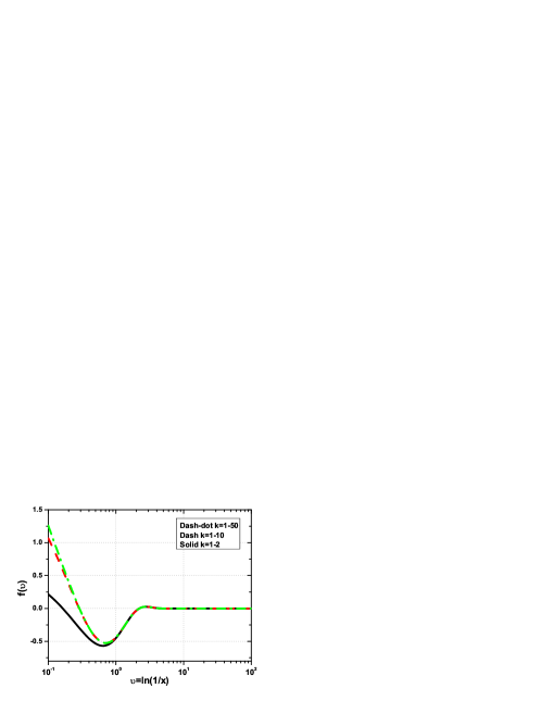
Figure 1: The function $\widehat{f}(\upsilon)$ [i.e., Eq.(20)] is plotted in a wide range of $\upsilon$. The solid black, dashed red, and dot-dashed green curves are shown according to the expansion of the second term in Eq.(20) in the ranges $k=1-2$, $k=1-10$, and $k=1-50$, respectively. The function $\widehat{f}(\upsilon)$ diverges as ln $\upsilon$ for $\upsilon\to 0$.

In Fig. 1, we analyze the function $\widehat{f}(\upsilon)$ in a wide range of $\upsilon$ according to the expansion of the second term in Eq. (20) in the ranges $k=1-2$, $k=1-10$, and $k=1-50$, respectively. We observe that the function $\widehat{f}(\upsilon)$ is very small as would be expected from the decreasing exponential factor in $\upsilon$ in Eq. (20). It is nearly independent of the cutoff in the expansion for $\upsilon\geq 1$, but the expansion must be carried to large $k$ for $\upsilon$ small. In the following we choose the value of $k=50$ in the numerical results.

In Fig. 2, using the parametrization for $F_{2}(x,Q^{2})$ in Eq. (3), we have plotted the longitudinal structure function $F_{L}(x,Q^{2})$ from Eq. (21) as a function of $x$ ($5{\times}10^{-5}<x<10^{-2}$) for the values of $Q^{2}=5,15,25$, and $45~{}\mathrm{GeV}^{2}$, respectively. In the figure, the H1 Collaboration data (H1 2011 [36] and H1 2014 [42]) accompanied by total errors for $Q^{2}=5,15,25$, and $45~{}\mathrm{GeV}^{2}$ are also shown.

In Fig. 3, we have separated our analysis of the longitudinal structure function at any fixed $Q^{2}$ and compare it with the results in [8] and [10] at the LO approximation as a function of $x$. The longitudinal structure function extracted at $Q^{2}$ values are in good agreement with experimental data in comparison with those in [8] at the LO approximation, as the mathematical structure of Eq. (8) in momentum space differs from the DGLAP equations for structure functions.

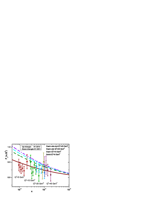
Figure 2: Plots of the longitudinal structure function $F_{L}(x,Q^{2})$ versus $x$ for $Q^{2}=5$ (solid brown), $15$ (dash green), $25$ (dash-dot turquoise), and $45~{}\mathrm{GeV}^{2}$ (dash-dot-dot purple), respectively. H1 Collaboration data are selected from [36](H1 2011) and [42](H1 2014).

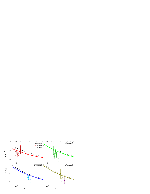
Figure 3: The longitudinal structure function $F_{L}(x,Q^{2})$ (solid curves) plotted at fixed $Q^{2}$ as a function of $x$ variable, compared with the Mellin transforms method [8] (dot curves) at the LO approximation. Experimental data (up-triangle H1 2014, down-triangle H1 2011) are from the H1-Collaboration [42, 36] as accompanied with total errors.

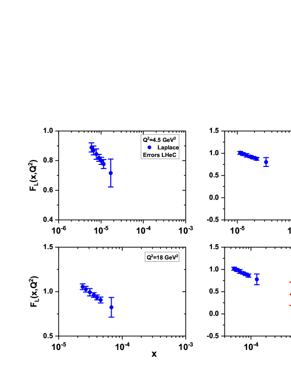
Figure 4: The central values of the longitudinal structure function are plotted at low $x$ as accompanied by the LHeC total errors [13]. H1 Collaboration data [36, 42] are collected at $Q^{2}=8.5$ and $35~{}\mathrm{GeV}^{2}$ with total errors.

In Fig. 4, the longitudinal structure functions in momentum space at selected $x$ and $Q^{2}$ are associated with the LHeC simulated uncertainties [13]. We observe that the longitudinal structure functions (central values) are determined owing to Eq. (21) for the $Q^{2}$ values (4.5, 8.5, 18, and 35$~{}\mathrm{GeV}^{2}$) and accompanied with the simulated uncertainties reported by the LHeC study group [13]. The H1 collaboration data with total errors for $Q^{2}=8.5$ and $35~{}\mathrm{GeV}^{2}$ are shown in Fig.4.

In Fig. 5, we show a comparison between the longitudinal structure functions in momentum space with the H1 Collaboration data at a fixed value of the invariant mass $W$ (i.e. $W=230~{}\mathrm{GeV}$) at low values of $x$. Figure 5 clearly demonstrates that the Laplace transform method in momentum space provides correct behaviors of the extracted longitudinal structure function in comparison with the LO and NLO analysis reported in [10]. As can be seen in this figure, the results are comparable with the H1 data and the NLO corrections to the Mellin transform method at all $Q^{2}$ values.

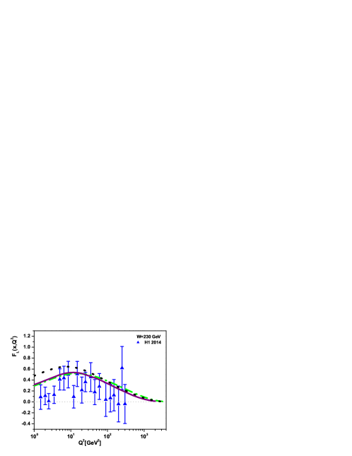
Figure 5: The extracted longitudinal structure function (solid brown curve) in momentum space at fixed value of the invariant mass $W$ ($W=230~{}\mathrm{GeV}$) compared with the H1 Collaboration data [42] as accompanied with total errors and the results in Refs. [8] and [10] at the LO (dotted black curve) and NLO (dot-dashed green curve) approximation.

V Conclusions

We have presented a method based on the Laplace transform method to determine the longitudinal structure function at the LO approximation in momentum space. This method relies on the parametrization of the function $F_{2}(x,Q^{2})$ and its derivative $dF_{2}(x,Q^{2})/d{\ln}Q^{2}$ within a kinematical region characterized by low values of the Bjorken variable $x$. The $x$ dependence of $F_{2}(x,Q^{2})$ and its evolution with $Q^{2}$ are determined much better by the data than $F_{L}(x,Q^{2})$, so this method provides both a direct check on $F_{L}(x,Q^{2})$ where measured, and a way of extending $F_{L}(x,Q^{2})$ into regions of $x$ and $Q^{2}$ where there are currently no data. We find that the Laplace transform method in momentum space provides correct behaviors of the extracted longitudinal structure function $F_{L}(x,Q^{2})$ and that our results for $F_{L}(x,Q^{2})$ demonstrate comparability with data from the H1 Collaboration and other results obtained using the Mellin transform method.

VI ACKNOWLEDGMENTS

G.R.Boroun thanks M.Klein and N.Armesto for allowing access to data related to simulated errors of the longitudinal structure function at the Large Hadron Electron Collider (LHeC). Phuoc Ha would like to thank Professor Loyal Durand for useful comments and invaluable support.

VII Appendix

The inverse Laplace transform

$$\widehat{f}(\upsilon)={\mathcal{L}^{-1}}\bigg{[}f(s),s;\upsilon\bigg{]}=\frac{1}{2\pi i}\int_{-i\infty}^{i\infty}dsf(s)e^{s\upsilon}$$ (22)

of the function

$$f(s)=\frac{(s+1)\psi(s+1)}{4+3s+s^{2}}$$ (23)

can be evaluated analytically in terms of an infinite series, rapidly convergent except for $\upsilon$ near zero where it grows logarithmically. The denominator in $f(s)$ has zeros at $s_{\pm}=-\frac{3}{2}\pm i\frac{\sqrt{7}}{2}$. which lead to simple poles in $f(s)$ at those points. The function $\psi(s+1)$ has simple poles with residue $-1$ at $s+1=0,-1,-2,...$ [44] . There are no other sigularities in the integrand which decreases exponentially rapidly for $s\rightarrow-\infty$ and Re$(\upsilon)>0$. We can therefore close the integration contour in the left-half $s$ plane and evaluate the integral as the sum of the residues at the poles multiplied by $2\pi i$ by Cauchy’s residue theorem.

This gives

$$\widehat{f}(\upsilon)=\frac{s_{+}+1}{s_{+}-s_{-}}\psi(s_{+}+1)e^{s_{+}\upsilon}-\frac{s_{-}+1}{s_{+}-s_{-}}\psi(s_{-}+1)e^{s_{-}\upsilon}+\sum_{k=1}^{\infty}\frac{k}{(k+1)^{2}-3(k+1)+4}e^{-(k+1)\upsilon}.$$ (24)

Since

$$\frac{s_{+}+1}{s_{+}-s_{-}}\psi(s_{+}+1)=-0.1704+1.211i\,,\,\,\,\,\,\frac{s_{-}+1}{s_{+}-s_{-}}\psi(s_{-}+1)=0.1704+1.211i.$$ (25)

we find

$$\widehat{f}(\upsilon)=-2e^{-\frac{3}{2}\upsilon}\bigg{[}0.1704\cos\big{(}\frac{\sqrt{7}}{2}\upsilon\big{)}+1.211\sin\big{(}\frac{\sqrt{7}}{2}\upsilon\big{)}\bigg{]}+\sum_{k=1}^{\infty}\frac{k}{(k+1)^{2}-3(k+1)+4}e^{-(k+1)\upsilon}.$$ (26)

For $\upsilon\ll 1$, $k$ large, the series is approximately

$$\sum_{k}\frac{1}{k}e^{-(k+1)\upsilon}\approx e^{-\upsilon}\,{\rm ln}\,(1-e^{-\upsilon}),$$ (27)

so diverges as ln $\upsilon$ for $\upsilon\to 0$.

Table 1: The effective parameters [7] at low $x$ for $0.15~{}\mathrm{GeV}^{2}<Q^{2}<3000~{}\mathrm{GeV}^{2}$.

parameters                    value
$a_{0}$	$8.205\times 10^{-4}~{}~{}\pm 4.62\times 10^{-4}$
$a_{1}$	$-5.148\times 10^{-2}\pm 8.19\times 10^{-3}$
$a_{2}$	$-4.725\times 10^{-3}\pm 1.01\times 10^{-3}$
$b_{0}$	$2.217\times 10^{-3}\pm 1.42\times 10^{-4}$
$b_{1}$	$1.244\times 10^{-2}\pm 8.56\times 10^{-4}$
$b_{2}$	$5.958\times 10^{-4}\pm 2.32\times 10^{-4}$
$c_{1}$	$1.475\times 10^{-1}~{}\pm 3.025\times 10^{-2}$
$n$	$11.49\pm 0.99$
$\lambda$	$2.430~{}\pm 0.153$
$M^{2}$	$0.753\pm 0.068~{}\mathrm{GeV}^{2}$
$\mu^{2}$	$2.82\pm 0.290~{}\mathrm{GeV}^{2}$
$c_{0}$	$0.255\pm 0.016$
$\chi^{2}(\mathrm{goodness~{}of~{}fit})$	$0.95$

References

- [1] T. Lappi, H. Mantysaari, H. Paukkunen and M.Tevio, Eur.Phys.J.C 84, 84 (2024).
- [2] V. N. Gribov and L. N. Lipatov, Sov.J.Nucl.Phys. 15, 438 (1972).
- [3] G. Altarelli and G. Parisi, Ncul.Phys.B 126, 298 (1977).
- [4] Y. L. Dokshitzer, Sov.Phys.JETP 46, 641 (1977).
- [5] B. Badelek, et al., J.Phys.G 22, 815 (1996).
- [6] S. Catani, F. Hautmann, Nucl.Phys.B 427, 475 (1994).
- [7] M. M. Block, L. Durand and P. Ha, Phys.Rev.D 89, 094027 (2014).
- [8] L.P. Kaptari, et al., JETP Lett. 109, 281 (2019).
- [9] G.R. Boroun, Phys.Rev.C 97, 015206 (2018).
- [10] L.P. Kaptari, et al., Phys.Rev.D 99, 096019 (2019).
- [11] G.R.Boroun and B.Rezaei, Phys.Lett.B 816, 136274 (2021).
- [12] M. Froissart, Phys. Rev. 123, 1053 (1961).
- [13] P.Agostini et al. [LHeC Collaboration and FCC-he Study Group], J. Phys. G: Nucl. Part. Phys. 48, 110501 (2021).
- [14] R. Abdul Khalek et al., Snowmass 2021 White Paper, arXiv [hep-ph]:2203.13199.
- [15] R.Abir et al., The case for an EIC Theory Alliance: Theoretical Challenges of the EIC, arXiv [hep-ph]:2305.14572.
- [16] M. Gluck, E. Reya, and A. Vogt, Z. Phys. C 48, 471 (1990).
- [17] W. Furmanski and R. Petronzio, Nucl. Phys. B 195, 237 (1982).
- [18] R. Toldra, Comput. Phys. Commun. 143, 287 (2002).
- [19] N. Cabibbo and R. Petronzio, Nucl. Phys. B 137, 395 (1978).
- [20] J.Rausch, V.Guzey and M.Klasen, Phys.Rev.D 107, 054003 (2023).
- [21] G.R.Boroun and B.Rezaei, Phys.Rev.D 105, 034002 (2022).
- [22] H.Khanpour, A.Mirjalili and S.Atashbar Tehrani, Phys.Rev.C 95, 035201 (2017).
- [23] G.R.Boroun, Eur.Phys.J.Plus 137, 32 (2022).
- [24] S.Atashbar Tehrani, F.Taghavi-Shahri, A.Mirjalili, M.M.Yazdanpanah, Phys.Rev.D 87, 114012 (2013).
- [25] S.Dadfar and S.Zarrin, Eur.Phys.J.C 80, 319 (2020).
- [26] M.Mottaghizadeh, P.Eslami and F.Taghavi-Shahri, Int.J.Mod.Phys.A 32, 1750065 (2017).
- [27] N.Olanj, M.Lotfi Parsa and L.Asgari, Phys.Lett.B 834, 137472 (2022).
- [28] R. D. Ball and S. Forte, Phys. Lett. B 336, 77 (1994).
- [29] A. V. Kotikov and G. Parente, Nucl. Phys. B 549, 242 (1999).
- [30] L. Mankiewicz, A. Saalfeld, and T. Weigl, Phys. Lett. B 393, 175 (1997).
- [31] M. Markovych and A. Tandogan, arXiv [hep-ph]:2304.10458.
- [32] A. Simonelli, arXiv [hep-ph]: 2401.13663.
- [33] M. M. Block and F. Halzen, Phys. Rev. D 70, 091901 (2004).
- [34] H. Abramowicz et al. (H1 and ZEUS Collaborations), Eur. Phys. J. C 78, 473 (2018).
- [35] V. Andreev et al. (H1 Collaboration), Eur. Phys. J. C 74, 2814 (2014).
- [36] F. D. Aaron et al. (H1 Collaboration), Eur. Phys. J. C 71, 1579 (2011).
- [37] Martin M. Block, Loyal Durand and Douglas W. McKay, Phys.Rev.D 79, 014031 (2009).
- [38] Martin M. Block, Loyal Durand, Phuoc Ha and Douglas W. McKay, Phys.Rev.D 83, 054009 (2011).
- [39] Martin M. Block, Loyal Durand, Phuoc Ha and Douglas W. McKay, Phys.Rev.D 84, 094010 (2011).
- [40] Martin M. Block, Loyal Durand, Phuoc Ha and Douglas W. McKay, Phys.Rev.D 88, 014006 (2013).
- [41] H1 and ZEUS Collaborations (H. Abramowicz et al.), Eur. Phys. J. C 78, 473 (2018).
- [42] H1 Collab. (V.Andreev et al.), Eur.Phys.J.C 74, 2814(2014).
- [43] M.A.G.Aivazis et al., Phys.Rev.D 50, 3102 (1994).
- [44] ”NIST Digital Library of Mathematical Functions” edited by F. W. J. Olver, A. B. Olde Daalhuis, D. W. Lozier, B. I. Schneider, R. F. Boisvert, C. W. Clark, B. R. Miller, B. V. Saunders, H. S. Cohl, and M. A. McClain, Sec. 5.2(i), https://dlmf.nist.gov/, Release 1.1.12 of 2023-12-15.