From Weak to Strong Sound Event Labels using Adaptive Change-Point Detection and Active Learning

Abstract

In this work we propose an audio recording segmentation method based on an adaptive change point detection (A-CPD) for machine guided weak label annotation of audio recording segments. The goal is to maximize the amount of information gained about the temporal activation’s of the target sounds. For each unlabeled audio recording, we use a prediction model to derive a probability curve used to guide annotation. The prediction model is initially pre-trained on available annotated sound event data with classes that are disjoint from the classes in the unlabeled dataset. The prediction model then gradually adapts to the annotations provided by the annotator in an active learning loop. The queries used to guide the weak label annotator towards strong labels are derived using change point detection on these probabilities. We show that it is possible to derive strong labels of high quality even with a limited annotation budget, and show favorable results for A-CPD when compared to two baseline query strategies.

I Introduction

Most audio datasets today consists of weakly labeled data with imprecise timing information [1], and there is a need for efficient and reliable annotation processes to acquire stronger labels with more precise timing information. The performance of sound event detection (SED) models improve with strong labels [2], and strong labels become especially important when we want to count the number of occurrences of an event class. For example in bioacoustics, where counting the number of vocalizations of an animal species can be used to estimate population density and drive ecological insights [3].

Crowdsourcing the strong labels is challenging and an attractive solution is to crowdsource weak labels to enable reconstruction of the strong labels [4, 5]. Asking the annotator for strong labels requires more work and it can in the worst case lead to the annotator misunderstanding the task [5].

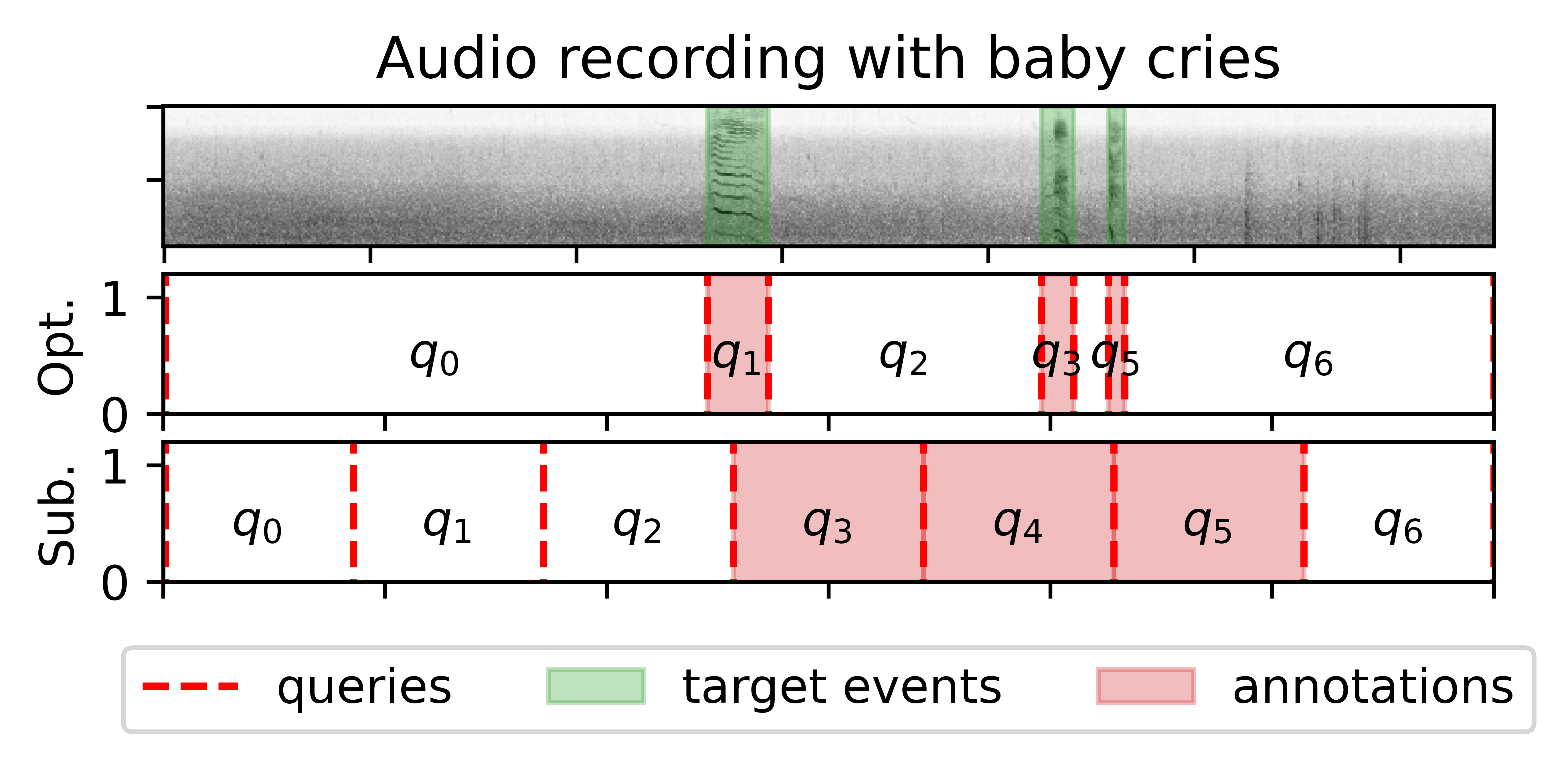
Figure 1: Illustration of segmentation of an audio spectrogram with three target events shown in shaded green (top panel) into a set of audio query segments $q_{0},\dots,q_{6}$ using an optimal method w.r.t the derived strong label timings (middle panel) and a sub-optimal method (bottom panel). Resulting annotations, from the weak labels given by the annotator, are shown in shaded red for both methods. Query $q_{4}$ for the optimal method is omitted for clarity.

Disagreement-based active learning is the most used form of active learning for sound event detection [6, 7, 8, 9], focusing on selecting what audio segment to label next. The recordings are either split into equal length audio segments [6, 7, 9] or segments depending on the structure of the sound [8]. Each segment is then given a weak label by the annotator.

In this work we use a weak label annotator to derive strong labels as in [5], but instead of using fixed length query segments we adapt the query segments to the data, in the setting of active learning. We propose an adaptive change point detection (A-CPD) method which splits a given audio recording into a set of audio segments, or queries. The queries are then labeled by an annotator and the strong labels are derived and evaluated. See Fig. 1 for an illustration of this concept, where a set of seven queries are used either optimally or sub-optimally for a given audio recording. We aim to adapt the set of queries in such a way that the information about the temporal activation’s of the target sounds is maximized. Note that this is different from the typical active learning setup in the sense that we aim to actively guide the annotator during the annotation of the audio recordings, rather than actively choose which audio recordings to annotate.

II Active learning for sound event detection

In this work we consider SED tasks where the goal is to predict the presence of a given target event class, but the results can also be generalized into the multi-class setting. We aim to train a SED system using active learning, given a restricted annotation budget and no initial labels. To this end, we propose the following active learning annotation process.

Let $\mathcal{D}^{(k)}_{L}$ denote the set of labeled audio recordings and $\mathcal{D}^{(k)}_{U}$ the set of unlabeled audio recordings at active learning iteration $k$. Further, let $\mathcal{A}^{(k)}=\{(s^{(j)}_{i},e^{(j)}_{i},c^{(j)}_{i})\}{{}_{i=1}^{B}}{{}_{j=1}^{k}}$ denote the annotations of segments, where $s$ denotes the onset, $e$ the offset, and $c\in\{0,1\}$, the weak label for each segment $i$ of the $B$ annotated segments in audio recording $j$.

We start without any labels, $\mathcal{A}^{(0)}=\mathcal{D}^{(0)}_{L}=\O$, and all audio recordings are unlabeled, $\mathcal{D}^{(0)}_{U}=\{\mathbf{x}_{j}\}_{j=1}^{N}$, where $\mathbf{x}_{j}\in\mathbb{R}^{T}$ denotes a audio recording of length $T$, and $N$ denotes the total number of audio recordings. We then loop for each $k\in\{1,\dots,N\}$ and:

1. choose a random unlabeled audio recording $\mathbf{x}$ from $\mathcal{D}^{(k-1)}_{U}$,

2. derive a set of $B$ audio query segments $Q=\{q_{i}\}_{i=0}^{B-1}$ using a query strategy where $q_{i}=(s_{i},e_{i})$ consists of the start $s_{i}$ and end $e_{i}$ timings for query $i$,

3. send the queries to the annotator (returning a weak label for each query) and add the annotations to the set of segment labels $\mathcal{A}^{(k)}=\mathcal{A}^{(k-1)}\cup\{(s_{i},e_{i},c_{i})\}_{i=1}^{B}$,

4. In case of A-CPD: use the annotations $\{(s_{i},e_{i},c_{i})\}_{i=1}^{B}$ to update the query strategy, and

5. update the labeled recording set $\mathcal{D}^{(k)}_{L}$ by adding $\mathbf{x}$ and the unlabeled recording set $\mathcal{D}^{(k)}_{U}$ by removing $\mathbf{x}$.

For brevity we have omitted the dependence on $k$ for $\mathbf{x}_{r_{k}}$ and $(s^{(r_{k})}_{i},e^{(r_{k})}_{i},c^{(r_{k})}_{i})$ in the description of the annotation loop, where $r_{k}\in\{1,\dots,N\}$ would denote the randomly sampled audio recording for iteration $k$. After the annotation loop all $N$ audio recordings have been annotated exactly once with the query method used in step (2), resulting in a set of annotations $\mathcal{A}^{(N)}=\{(s^{(j)}_{i},e^{(j)}_{i},c^{(j)}_{i})\}{{}_{i=1}^{B}}{{}_{j=1}^{N}}$.

The total annotation budget used will scale with both $N$ and $B$. A typical active learning setup would aim to minimize $N$ while maintaining test time model performance, where in this work we instead aim to minimize $B$. In this way we can reduce the annotation budget and increase the annotation quality without introducing a selection bias for the labeled audio recordings, since all recordings are labeled. Think of $B$ as the annotation cost of the annotator, which is minimized by guiding the annotator during the annotation process.

III Query strategies

In this section we describe the studied query strategies.

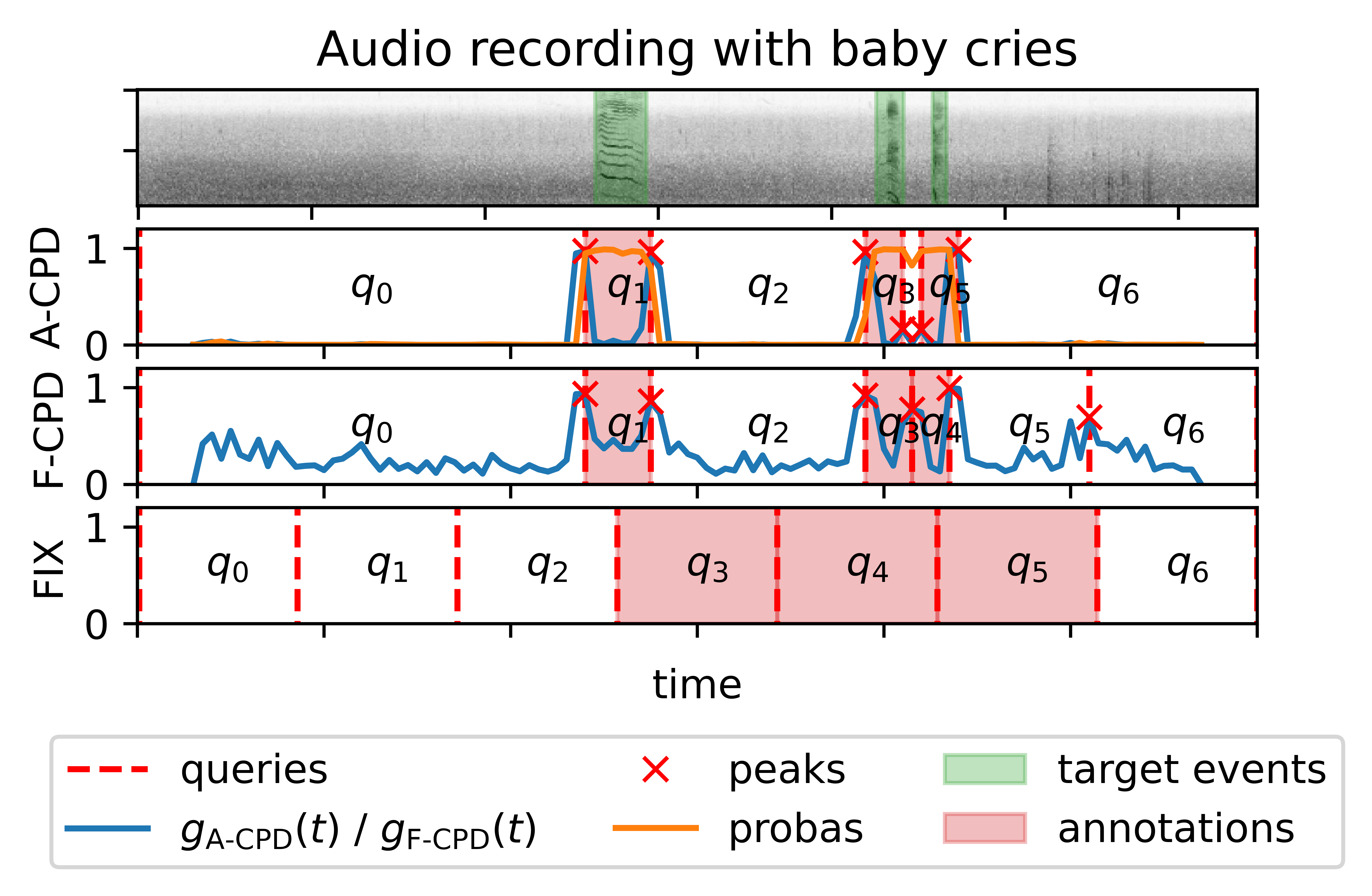
Figure 2: Illustration of how the different query strategies A-CPD, F-CPD and FIX segment a spectrogram of an audio recording with three target events shown in shaded green (top panel) into $B=7$ queries. A-CPD (second panel) uses change point detection (blue line) on the probability curve from a prediction model (orange line) to detect the $B-1$ most prominent peaks (red crosses) which are used to construct a set of queries $\{q_{0},\dots,q_{B-1}\}$ (dashed red lines). Each query $q_{i}=(s_{i},e_{i})$ is given a weak label $c_{i}\in\{0,1\}$ ($c=1$ shown as shaded red), resulting in the $i$:th annotation $(s_{i},e_{i},c_{i})$. F-CPD (third panel) uses change point detection directly on the cosine similarities in embedding space (blue line) and thereafter constructs queries in the same way as A-CPD. FIX (fourth panel) uses fixed length queries.

III-A The adaptive change point detection strategy (A-CPD)

To produce a set of queries for a given audio recording $\mathbf{x}$ at annotation round $k$ we perform three key steps:

1. update a prediction model using the annotations from round $k-1$ (initialized with pre-training if $k=0$),

2. predict probabilities indicating the presence of the target class in the recording using the model, and

3. apply change point detection to the probabilities to derive the queries.

The pre-training of the prediction model can be done in a supervised or unsupervised way. The important property is that the model reacts to changes in the audio recording related to the presence or absence of the target class. However, it is not strictly necessary that the model reacts only to those changes.

Let $h_{k}:\mathbb{R}^{L}\rightarrow[0,1]$ denote a model that predicts the probability of an audio segment of length $L$ belonging to the target event class. In principle, any prediction model can be used. For a given audio recording $\mathbf{x}$ the prediction model $h_{k}(\cdot)$ is applied to consecutive audio segments to derive a probability curve, shown as the orange curve for A-CPD in Fig. 2. The consecutive audio segments are derived using a moving window of $L$ seconds with hop size $L/4$.

We define the Euclidean distance between two points $t-\alpha$ and $t+\alpha$ on the probability curve as:

$$g^{(k)}_{\text{A-CPD}}(t)=||h_{k}(t-\alpha)-h_{k}(t+\alpha)||_{2}^{2},$$ (1)

shown as the blue curve for A-CPD in Fig. 2. The previous probability is compared with the next probability in Eq. 1, and $\alpha=L/4$ (hop size) is therefore chosen to ensure a $50$% overlap between the audio segments for these probabilities.

Let $t$ be a local optimum of $g^{(k)}_{\text{A-CPD}}(t)$, and all such local optima are called peaks. We rank peaks based on prominence. For any given peak $t$, let $t_{l}$ and $t_{r}$ denote the closest local minima of $g_{k}(\cdot)$ to the left and right of $t$. The prominence of the peak at $t$ is defined as $|g_{k}(t)-\max(g_{k}(t_{l}),g_{k}(t_{r}))|$. Let $\mathcal{T}_{\text{A-CPD}}=\{t_{1},t_{2},\dots,t_{B-1}\}$ be the $B-1$ most prominent peaks of a given audio recording such that $t_{1}\leq t_{2}\leq\dots\leq t_{B-1}$, shown as red crosses in Fig. 2. The A-CPD query method is then defined as:

$$Q^{(k)}_{\text{A-CPD}}=\{(0,t_{1}),(t_{1},t_{2}),\dots,(t_{B-1},T)\},$$ (2)

which are shown as dashed red lines in Fig. 2, where $T$ is the length of the audio recording and $B$ is the number of queries used. Note that $g^{(k)}_{\text{A-CPD}}(t)$ will gradually become more sensitive towards changes between presence and absence of the target class in the recording with additional annotations, and become less sensitive to other unrelated changes.

III-B The fixed change point detection strategy (F-CPD)

The fixed change point detection (F-CPD) method used as a reference derives the queries by computing the cosine similarity between the previous embedding at time $t-\alpha$ and the next embedding at time $t+\alpha$:

$$g_{\text{F-CPD}}(t)=\frac{\mathbf{e}_{t-\alpha}\cdot\mathbf{e}_{t+\alpha}}{||\mathbf{e}_{t-\alpha}||||\mathbf{e}_{t+\alpha}||},$$ (3)

where $\mathbf{e}_{t}=f_{\theta}(\mathbf{x}_{t})$ denotes the embedding of consecutive audio segments $\mathbf{x}_{t}$ centered at second $t$ using the embedding function $f_{\theta}:\mathbb{R}^{L}\rightarrow\mathbb{R}^{K}$. The cosine similarity curve for an audio recording is shown as the blue line for F-CPD in Fig. 2. This method is similar to [8] except that embeddings are derived for $1.0$ seconds of audio instead of $0.02$. We therefore directly compare the previous and next embeddings instead of a moving average as in [8].

The most prominent peaks in the cosine similarity curve is then selected, $\mathcal{T}_{\text{FIX}}=\{t_{1},t_{2},\dots,t_{B-1}\}$, and the set of queries are defined as in Eq. 2, shown as dashed red lines for F-CPD in Fig 2.

III-C The fixed length strategy (FIX)

In the fixed length query strategy (FIX) audio is split into equal length segments and then labeled. Let $d=T/B$, then the queries are defined as

$$Q_{\text{FIX}}=\{(0d,1d),(1d,2d),\dots,((B-1)d,Bd)\},$$ (4)

shown as dashed red lines for FIX in Fig 2. This is the setting most previous active learning work for SED consider.

III-D Oracle query strategy (ORC)

The oracle query strategy constructs the queries based on the ground truth presence and absence annotations

$$Q_{\text{ORC}}=\{(s_{0},e_{0}),(s_{1},e_{1}),\dots,(s_{B_{\text{suff}}-1},e_{B_{\text{suff}}-1})\},$$ (5)

where $(s_{i},e_{i})$ is the onset and offset for segment $i$ where the target event is either present or not. $B_{\text{suff}}$ is the sufficient number of queries to get the true strong labels, which relate to the number of target events $M$ in the given audio recording by $B_{\text{suff}}=2M+1$. ORC is undefined for $B<B_{\text{suff}}$.

III-E The role of query strategies in the annotation process

The query strategies described in this section are then used in step (2) of the annotation loop described in Section II. Note that when the queries are not adapted to the audio recording multiple events can end up being counted as one. In Fig. 2 we can see this for F-CPD where $q_{3}$ and $q_{4}$ are directly adjacent, meaning that they are not resolved as two separate events, and for FIX where $q_{3}$, $q_{4}$ and $q_{5}$ are all directly adjacent. A-CPD resolves all three events.

The FIX length query segments depend on the query timings and target event timings aligning by chance since the query construction is independent of the target events. The A-CPD method aim to create query segments that are aligned with the target events by construction. In addition the number of queries needed to derive the strong labels scale with the number of target events in the recording for A-CPD, which can be beneficial.

IV Evaluation

IV-A Datasets

We create three SED datasets for evaluation, each with a different target event class: Meerkat, Dog or Baby cry. The Meerkat sounds are from the DCASE 2023 few-shot bioacoustic SED dataset [10] and the Dog and Baby cry sounds from the NIGENS dataset [11]. The sounds used for absence of an event are from the $15$ background types in the TUT Rare sound events dataset [12].

The audio recordings in each dataset are created by randomly selecting $M=3$ sound events from that event class and mixing them together with a randomly selected background recording of length $T=30$ seconds. In this way we know that exactly $B_{\text{suff}}=2M+1=7$ queries are sufficient and necessary to derive the ground truth strong labels using a weak label annotator. The mixing is done using Scaper [13] at an SNR of $0$ dB. In total we generate $N=300$ audio recordings using this procedure for each event class class as training data and equally many as test data.

The source files used in the mixing uses the supplied splits in [11] and [12], except for the Meerkat sounds where non exist and the split is done on a recording level.

IV-B Evaluation metrics

We evaluate the methods by annotating the mixed training datasets using the query strategies described in Section II and the annotation loop described in Section III. The quality of the annotations are then measured in two ways: (i) how strong the annotations are compared to the ground truth, and (ii) the test time performance of two evaluation models trained using the different annotations.

The evaluation metrics used in case (i) and (ii) are event-based $F_{1}$-score ($F_{1e}$) and segment-based $F_{1}$-score ($F_{1s}$) [14]. The segment size for $F_{1s}$ is set to $0.05$ seconds, and the collar for $F_{1e}$ is set to $0.5$ seconds. In case (i) the $F_{1s}$ measures how much of the audio that has been correctly labeled and in case (ii) $F_{1s}$ measures how much of the audio that has been correctly predicted by the evaluation model. The $F_{1e}$ score is only used to measure how close the annotations are to the ground truth labels in the training data.

Annotator model

Let $\mathcal{A}^{(j)}_{gt}=\{(s_{i},e_{i},c=1)\}{{}_{i=1}^{3}}$ denote the set of ground truth target event labels for audio recording $j$, where $s_{i}$ is the onset, $e_{i}$ the offset and $c=1$ indicate the presence of the target event.

We use $\mathcal{A}^{(j)}_{gt}$ to simulate an annotator for recording $j$. For a given query segment we check the overlap ratio with the ground truth target event labels. Formally, if there exists an annotation $(s_{i},e_{i},c_{i}=1)$ s.t.

$$\frac{(s_{i},e_{i})\cap(s_{q},e_{q})}{|s_{i}-e_{i}|}\geq\gamma,$$ (6)

holds for the given query segment $q=(s_{q},e_{q})$, then the annotator returns $c_{i}=1$ for query $q$, and $c_{i}=0$ otherwise. Annotation noise is added by flipping the returned label with probability $\beta$. In this work $\gamma=0.5$, and $\beta\in\{0.0,0.2\}$.

IV-C Implementation details and experiment setup

Prediction model

The prediction model $h_{k}(\cdot)$ is modeled using a prototypical neural network (ProtoNet) [15]. The prototypes are easily updated at each annotation round $k$ using a running average between each previous prototype and the newly labeled audio embeddings. We model the embedding function $f_{\theta}(\cdot)$ using BirdNET [16], a convolutional neural network pre-trained on large amounts of bird sounds.

Evaluation models

We use two models to evaluate the test time performance of models trained on the annotations obtained using each query strategy: a two layer multilayer perceptron (MLP) and a ProtoNet. The MLP is trained using the Adam optimizer and cross-entropy loss. Each query strategy is run $10$ times and the evaluation models are trained on the embeddings using the resulting labeled datasets. ProtoNet is used in two ways: as a prediction model in the proposed A-CPD method, and as an evaluation model.

IV-D Results

In Table I we show the average $F_{1s}$-score and $F_{1e}$-score for the training data annotations over $10$ runs for each dataset and with the sufficient budget $B=B_{\text{suff}}=7$. The A-CPD method outperforms the other methods for all studied target event classes. The standard deviation is in all cases less than $0.03$ (omitted from table for brevity), and the baseline query strategies are deterministic when $\beta=0$.

Strategy	Meerkat		Dog		Baby
	$F_{1s}$	$F_{1e}$	$F_{1s}$	$F_{1e}$	$F_{1s}$	$F_{1e}$
ORC	$1.00$	$1.00$	$1.00$	$1.00$	$1.00$	$1.00$
A-CPD	$\mathbf{0.31}$	$\mathbf{0.57}$	$\mathbf{0.29}$	$\mathbf{0.45}$	$\mathbf{0.62}$	$\mathbf{0.60}$
F-CPD	$0.16$	$0.44$	$0.21$	$0.30$	$0.48$	$0.45$
FIX	$0.11$	$0.00$	$0.19$	$0.00$	$0.41$	$0.01$

TABLE I: Average $F_{1s}$-score and $F_{1e}$-score for the training annotations for each annotation process and target event class with $\beta=0$

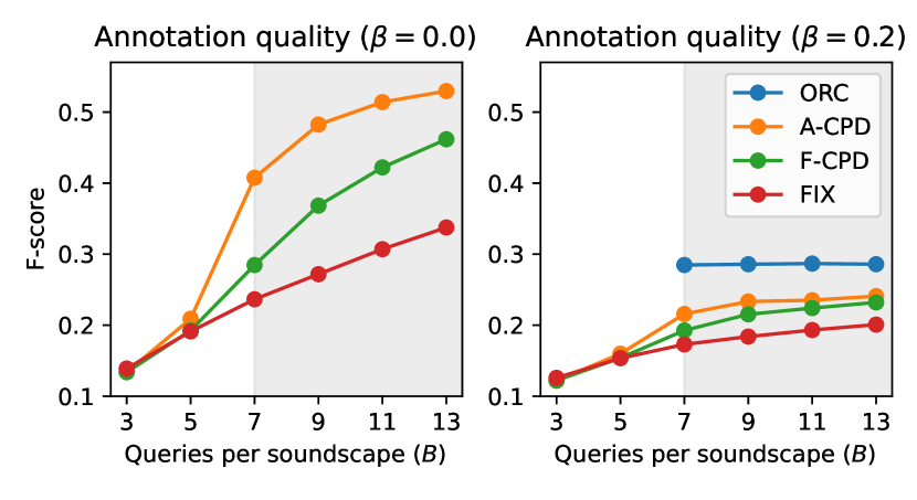
Figure 3: The average $F_{1s}$-score over the three classes for each of the studied annotation processes plotted against the number of queries per audio recording, $B$. The results are shown for an annotator without noise (left) and with $\beta=0.2$ (right). Note that ORC is $1.0$ when $\beta=0$ and is therefore not shown in the left figure. Shaded region where $B\geq B_{\text{suff}}$.

In Fig. 3 we show the average $F_{1s}$-score over all runs and event classes for the annotations derived from each query strategy. The proposed A-CPD method has a strictly higher $F_{1s}$-score than the FIX and F-CPD baselines for all budgets and noise settings. We also see that there is still a significant gap to the ORC strategy. The noisy annotator ($\beta=0.2$) drastically reduce the label quality for all studied strategies, especially ORC dropping from an $F_{1s}$-score of $1.0$ (omitted from figure) to $\approx 0.28$.

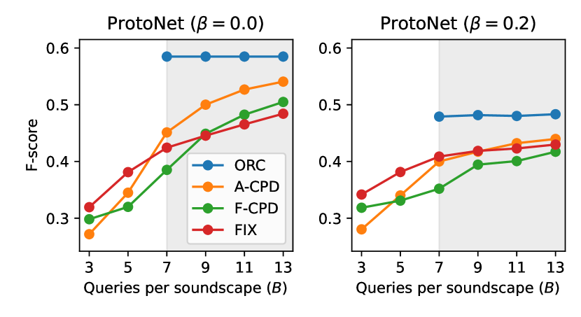
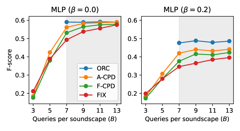
Figure 4: The average test time $F_{1s}$-score over the studied sound classes for a ProtoNet (top) and the MLP (bottom) trained with the annotations from each respective annotation process and setting. Shaded region where $B\geq B_{\text{suff}}$.

In Fig. 4 we show the average test time $F_{1s}$-score of a ProtoNet (top) and a MLP (bottom) trained using the annotations from each of the studied annotation strategies and settings. The A-CPD method outperforms the other methods when $B\geq 7$. For the ProtoNet the FIX method outperform A-CPD when $B<7$ and for the MLP the results are similar.

Table II and III show the average $F_{1s}$-score and standard deviation for the three different event classes for all studied query strategies. The average is over $10$ runs, and the number of queries is set to $B=7$.

Table II shows the $F_{1s}$-score for the ProtoNet evaluation model. A-CPD achieves a higher $F_{1s}$-score for the meerkat and baby datasets, but FIX performs better for the dog dataset. Note that on average A-CPD outperforms the other methods as seen in Fig. 4.

Strategy	Meerkat	Dog	Baby
ORC	$0.46$	$0.48$	$0.81$
A-CPD	$\mathbf{0.44}\pm 0.00$	$0.20\pm 0.01$	$\mathbf{0.71}\pm 0.02$
F-CPD	$0.31$	$0.19$	$0.66$
FIX	$0.34$	$\mathbf{0.25}$	$0.68$

TABLE II: Average test time $F_{1s}$-score for ProtoNet with $\beta=0$.

Table III shows the $F_{1s}$-score for the MLP evaluation model. A-CPD achieves a higher $F_{1s}$-score for all studied datasets.

Strategy	Meerkat	Dog	Baby
ORC	$0.43\pm 0.00$	$0.51\pm 0.01$	$0.83\pm 0.00$
A-CPD	$\mathbf{0.44}\pm 0.00$	$\mathbf{0.43}\pm 0.02$	$\mathbf{0.81}\pm 0.01$
F-CPD	$0.38\pm 0.01$	$0.42\pm 0.02$	$0.79\pm 0.01$
FIX	$0.33\pm 0.02$	$0.40\pm 0.02$	$0.75\pm 0.02$

TABLE III: Average test time $F_{1s}$-score for MLP with $\beta=0$.

IV-E Discussion

The results in all tables are for the sufficient budget $B=B_{\text{suff}}=2M+1$. In practice we do not know $B_{\text{suff}}$, and estimating $B_{\text{suff}}$ based on the audio recording is interesting future work. In that way we could further minimize the number of queries used for each audio recording, and thus decrease the annotation cost.

However, the A-CPD method is as applicable as any of the other baseline methods also for an arbitrary number of events in the recording even without an estimate of $B_{\text{suff}}$ for sufficiently large fixed $B$.

We chose $\gamma=0.5$ in the annotator model since the annotator should be able to detect a target event if more than $50$% of the event occurs within the query segment. This assumption about the annotators capacity is however non-trivial, and depends on the annotator and target class among others. We observe similar results as those presented in the paper on average for $\gamma\in\{0.05,0.25,0.5,0.75,0.95\}$ (not shown).

We use BirdNET [16] to model the embedding function since we study bioacoustic target classes. However, an embedding function such as PANNs [17] may also be used if the target classes are more general.

V Conclusions

In this work we have presented a query strategy based on adaptive change point detection (A-CPD) which derive strong labels of high quality from a weak label annotator in an active learning setting. We show that A-CPD gives strictly stronger labels than all other studied baseline query strategies for all studied budget constraints and annotator noise settings. We also show that models trained using annotations from A-CPD tend to outperform models trained with the weaker labels from the baselines at test time. We note that the gap to the oracle method is still large, so there is still ample room for improvements in future work.

References

- [1] Q. Kong, Y. Xu, W. Wang, and M. D. Plumbley, “Sound event detection of weakly labelled data with cnn-transformer and automatic threshold optimization,” IEEE/ACM Transactions on Audio, Speech, and Language Processing, vol. 28, pp. 2450–2460, 2020.
- [2] S. Hershey, D. P. Ellis, E. Fonseca, A. Jansen, C. Liu, R. C. Moore, and M. Plakal, “The benefit of temporally-strong labels in audio event classification,” ICASSP, IEEE International Conference on Acoustics, Speech and Signal Processing - Proceedings, pp. 366–370, 2021.
- [3] T. A. Marques, L. Thomas, S. W. Martin, D. K. Mellinger, J. A. Ward, D. J. Moretti, D. Harris, and P. L. Tyack, “Estimating animal population density using passive acoustics,” Biological Reviews, vol. 88, no. 2, pp. 287–309, 2013. [Online]. Available: https://onlinelibrary.wiley.com/doi/abs/10.1111/brv.12001
- [4] I. Martin-Morato, M. Harju, and A. Mesaros, “Crowdsourcing Strong Labels for Sound Event Detection,” IEEE Workshop on Applications of Signal Processing to Audio and Acoustics, pp. 246–250, 2021.
- [5] I. Martin-Morato and A. Mesaros, “Strong Labeling of Sound Events Using Crowdsourced Weak Labels and Annotator Competence Estimation,” IEEE/ACM Transactions on Audio Speech and Language Processing, vol. 31, pp. 902–914, 2023.
- [6] Z. Shuyang, T. Heittola, and T. Virtanen, “Active learning for sound event classification by clustering unlabeled data,” ICASSP, IEEE International Conference on Acoustics, Speech and Signal Processing - Proceedings, pp. 751–755, 2017.
- [7] ——, “An active learning method using clustering and committee-based sample selection for sound event classification,” 16th International Workshop on Acoustic Signal Enhancement, IWAENC 2018 - Proceedings, pp. 116–120, 2018.
- [8] ——, “Active Learning for Sound Event Detection,” IEEE/ACM Transactions on Audio Speech and Language Processing, vol. 28, pp. 2895–2905, 2020.
- [9] Y. Wang, M. Cartwright, and J. P. Bello, “Active Few-Shot Learning for Sound Event Detection,” Proceedings of the Annual Conference of the International Speech Communication Association, INTERSPEECH, pp. 1551–1555, 2022.
- [10] I. Nolasco, S. Singh, E. Vidana-Villa, E. Grout, J. Morford, M. Emmerson, F. Jensens, H. Whitehead, I. Kiskin, A. Strandburg-Peshkin, L. Gill, H. Pamula, V. Lostanlen, V. Morfi, and D. Stowell, “Few-shot bioacoustic event detection at the DCASE 2022 challenge,” no. November, pp. 1–5, 2022.
- [11] I. Trowitzsch, J. Taghia, Y. Kashef, and K. Obermayer, “NIGENS general sound events database,” Feb. 2019. [Online]. Available: https://doi.org/10.5281/zenodo.2535878
- [12] A. Diment, A. Mesaros, T. Heittola, and T. Virtanen, “TUT Rare sound events, Development dataset,” Jan. 2018. [Online]. Available: https://doi.org/10.5281/zenodo.401395
- [13] J. Salamon, D. MacConnell, M. Cartwright, P. Li, and J. P. Bello, “Scaper: A library for soundscape synthesis and augmentation,” IEEE Workshop on Applications of Signal Processing to Audio and Acoustics, pp. 344–348, 2017.
- [14] A. Mesaros, T. Heittola, and T. Virtanen, “Metrics for polyphonic sound event detection,” Applied Sciences (Switzerland), vol. 6, no. 6, 2016.
- [15] J. Snell, K. Swersky, and R. Zemel, “Prototypical networks for few-shot learning,” Advances in Neural Information Processing Systems, pp. 4078–4088, 2017.
- [16] S. Kahl, C. M. Wood, M. Eibl, and H. Klinck, “BirdNET: A deep learning solution for avian diversity monitoring,” Ecological Informatics, vol. 61, no. January, p. 101236, 2021.
- [17] Q. Kong, Y. Cao, T. Iqbal, Y. Wang, W. Wang, and M. D. Plumbley, “Panns: Large-scale pretrained audio neural networks for audio pattern recognition,” IEEE/ACM Transactions on Audio, Speech, and Language Processing, vol. 28, pp. 2880–2894, 2020.