2Lancaster Environment Centre, Lancaster University, United Kingdom
3Department of Mathematics and Statistics, Lancaster University, United Kingdom
4School of Mathematical Sciences, University College Cork, Ireland
Spatial Latent Gaussian Modelling with Change of Support
Abstract
[Data integration, Gaussian processes, geo-additive models, land suitability, model-based geostatistics, spatial misalignment.] Spatial data are often derived from multiple sources (e.g. satellites, in-situ sensors, survey samples) with different supports, but associated with the same properties of a spatial phenomenon of interest. It is common for predictors to also be measured on different spatial supports than the variables making up the response. Although there is no standard way to work with spatial data with different supports, a prevalent approach used by practitioners has been to use downscaling or interpolation to project all the variables of analysis towards a common support, and then using standard spatial models on this common support. The main disadvantage with this approach is that simple interpolation can introduce biases and, more importantly, the uncertainty associated with the change of support is not taken into account in the parameter estimation of the main model of interest. In this article, we propose a Bayesian spatial latent Gaussian model that can handle data with different rectilinear supports in the response variable and the predictors. Our approach allows us to handle changes of support more naturally according to the properties of the spatial stochastic process being used, and to take into account the uncertainty from the change of support in parameter estimation and prediction. We use spatial stochastic processes as linear combinations of basis functions where Gaussian Markov random fields define the weights. This process can be projected to different supports whilst maintaining the same parameters. Our hierarchical modelling approach can be described by the following steps: (i) define a latent model where response variables and predictors are considered as latent stochastic processes with continuous support, (ii) link the continuous-index set stochastic processes with its projection to the support of the observed data, (iii) link the projected process with the observed data. We show the applicability of our approach by simulation studies and modelling the land suitability of improved grassland in Rhondda Cynon Taf, a county borough in Wales.
1 Introduction
Many research questions in environmental science and public health necessitate the utilisation of heterogeneous spatial data encompassing different supports. The characteristics of the support, commonly referred to as spatial sampling units, can vary significantly across data sources, including variations in size, shape, spacing, and extent (Dungan et al.,, 2002). In disease incidence and prevalence modelling, it is common to obtain case data at multiple levels of aggregation, such as at the individual level, census areas, counties, and districts, along with predictors observed at both individual and aggregated levels, including satellite pixels (Wang et al.,, 2018; Alegana et al.,, 2016; Lee and Anderson,, 2022). In environmental modelling, there is also a frequent need to combine information from data sources with different supports across both the response and predictor variables, with a particular emphasis on the use of satellite products and synthetic data derived from climate models (Brown et al.,, 2022; Pacifici et al.,, 2019; Ma and Kang,, 2020). Integrating different data sources to address a research question offers the potential to enhance parameter estimation and improve prediction accuracy (Wang et al.,, 2018; Pacifici et al.,, 2019; Law et al.,, 2018; Leopold et al.,, 2006). However, to achieve reliable results, it is crucial to employ a data fusion framework that appropriately acknowledges the support of the data and incorporates reasonable assumptions to mitigate biases and accurately quantify uncertainty (Gotway and Young,, 2002; Pacifici et al.,, 2019).
The process of projecting observed data to a common support, known as change of support (COS) in spatial statistics, is essential when integrating heterogeneous data with different supports. This encompasses two key situations: the change of support problem (COSP), where the response variable is observed at different supports, and spatial misalignment, where the support of predictors and responses differ (Gelfand et al.,, 2001; Gotway and Young,, 2002; Zhu et al.,, 2003). Both scenarios require addressing the challenge of effectively utilising the information from different sources and aligning the data appropriately. In this paper, we adopt the term change of support to encompass both situations, highlighting the importance of expressing the projection of spatial data to a specific support within a unified framework for data integration and handling spatial misalignment.
Numerous attempts have been made to address the change of support problem in order to integrate multiple spatial data sources. The first set of approaches focuses on geostatistical methods, including point-to-point, block-to-block, point-to-block, and block-to-point Kriging (Kyriakidis,, 2004). These methods involve computing the covariance matrix using Monte Carlo integration and parameter estimation through variogram fitting. When dealing with spatial misalignment, predictors are projected to the response support using one of the types of Kriging and incorporated into regression models (Young et al.,, 2009).
The second set of approaches utilises Gaussian processes, a widely applied tool in spatial statistics, to tackle the change of support problem. Several strategies exist within this framework. One common approach is similar to Kriging, where the covariance matrix is computed using Monte Carlo integration (Gelfand et al.,, 2001). Inference under the Gaussian process framework typically involves optimising the likelihood function or utilising Bayesian inference. Another strategy involves incorporating spatial point-level auxiliary variables, approximating the integral of the Gaussian process over a region by averaging the spatial auxiliary variables within that region (Cowles et al.,, 2009). The objective here is to obtain the posterior distribution of these auxiliary variables. Additionally, a multivariate approach can be employed, treating all variables as responses and defining a full covariance matrix between sources. This approach leverages separable covariances to reduce computational costs and approximates the covariance structure on aggregated supports using Monte Carlo integration (Finley et al.,, 2014). Predictions can be made for all responses or specific ones. An alternative spectral approach, proposed by Reich et al., (2014), utilises the spectral representation of a Gaussian process. The model at aggregated support resembles a linear model with pseudo-predictors derived from spectral analysis. Finally, a computationally efficient approach involves utilising stochastic partial differential equations (SPDE) to approximate the aggregated Gaussian process (Moraga et al.,, 2017). The representation of the aggregated GP using SPDE has a similar structure as the continuous GP with a custom linear transformation. With this approximation, the methods for spatial inference and prediction using SPDE can be applied.
The third set assumes that data arise from processes that are piecewise constant on a predefined grid. This allows for analytical simplification, where integrals become linear combinations of areas. The projection of piecewise processes to other supports is computed as weighted averages of the latent process values at cells intersecting the area of interest. These approaches often utilise grids based on the highest observed resolution or custom computational grids. The main objective is to obtain the posterior distribution of the piecewise constant process (Taylor et al.,, 2015, 2018; Bradley et al.,, 2016).
Although various approaches have been developed to address the change of support problem using Kriging, Gaussian processes, and piecewise processes, they are not without limitations. Many of these approaches rely on approximating covariance matrices on aggregated supports using Monte Carlo integration or by averaging spatial random variables. However, the accuracy of these approximations depends on the number of points used and the sampling algorithms employed, and the discussion of approximation errors is often neglected. Moreover, these approximations are necessary even in simpler domains like regular and rectilinear grids. Another limitation is the lack of a precise connection between the continuous and aggregated spatial processes in some approaches. Lastly, most existing approaches are tailored to specific types of models, which restricts their flexibility in handling more complex modelling scenarios within a unified framework.
In this article, we propose a Bayesian latent Gaussian spatial model that addresses the challenge of handling data with different supports in the response variable and predictors. Our approach offers a more natural and flexible way to handle the change of support problem, taking into account the properties of the underlying spatial stochastic process. We incorporate the uncertainty associated with the change of support into parameter estimation and prediction. Our proposed model utilises a spatial stochastic process expressed as a linear combination of basis functions, where the weights are determined by Gaussian Markov random fields. Notably, this process allows for accurate projection onto rectilinear supports while preserving the same set of parameters. The hierarchical nature of our model involves the following steps: (i) defining a latent model using latent stochastic processes with continuous support that are related to the response variables and predictors, (ii) establishing the connection between the continuous-index set stochastic processes and their projection onto the support of the observed data, and (iii) linking the observed data as noisy realisations of the projected processes. We demonstrate the practical application of our approach in modelling the land suitability of improved grassland in Rhondda Cynon Taf, a county borough in Wales. Our prediction of land suitability relies on various predictors, including elevation, growing degree days, and soil moisture surplus. Notably, these predictors are available at different resolutions than the land cover data (25).
The paper is structured as follows. In Section 2, we introduce spatial latent Gaussian models as a comprehensive framework encompassing common models used in spatial statistics. Section 3 builds upon this foundation and extends the discussion to the properties of these processes when projected onto aggregated supports. We present our proposed Bayesian latent Gaussian spatial model with change of support in this section. To demonstrate the reliability and flexibility of our approach, we conduct simulation studies in Section 4. In Section 5, we model the land suitability of improved grassland in Rhondda Cynon Taf. Finally, in Section 6, we discuss the contributions, advantages, disadvantages, limitations, and potential future directions of our work.
2 Spatial latent Gaussian models
Spatial latent Gaussian models (SLGM) encompass commonly used models for analysing spatial point-level and area-level data. They can be tailored to specific classical generalised spatial models depending on the latent stochastic process used to capture spatial variation. We define a SLGM in Section 2.1 and discuss the limitations concerning their ability to handle spatial data with different levels of support in Section 2.2.
2.1 Definition
A classical SLGM assumes that the conditional distribution of a random function , for a location , given a -dimensional set of covariates and the Gaussian random function , can be defined as follows
| (1) |
where is the link function between the conditional mean and the linear predictor , and is an additional parameter. As usual, and are the intercept and covariate effects, respectively. For a set of locations , which can be points, lines or regions, this implies that the elements of a set of random variables are conditionally independent given the covariates and the spatial stochastic process . This model assumes that the random vector follows a multivariate Gaussian distribution.
The model defined by the Equation (2.1) encompasses various classical spatial models based on the specific type of (point or regions) and the properties of the spatial stochastic process . There are three main cases: i) In the classical generalised geostatistical model, represents a point, and is defined as a Gaussian process with zero-mean and covariance function . ii) In the generalised conditional autoregressive (CAR) spatial model, represents a region and is defined as a Gaussian Markov random field (GMRF) with zero-mean and precision matrix . iii) In the geoadditive model, represents a point, and is defined using basis functions. Details of common stochastic processes can be found in Section B.1 of the Supplementary Material (SM).
2.2 Limitations
Although the framework defined by Equation (2.1) is attractive and encompasses different types of spatial models, it has certain requirements. Firstly, it assumes that responses are observed at the same type of support, such as either point-level or aggregated-level data. Secondly, both responses and predictors need to be available at the same sampling units to make inferences. Lastly, predictors should be available for any location within the area of interest () to enable spatial prediction at unobserved locations. However, these assumptions are often challenging to satisfy in real-world applications and are closely tied to the concept of change of support discussed earlier.
In practice, it is common for practitioners to perform pre-processing steps when using the models defined in Equation 2.1. This is because the three assumptions mentioned earlier are often not met, and existing approaches for dealing with change of support are often inflexible. These approaches typically involve approximating covariance matrices on aggregated supports using Monte Carlo integration or by averaging spatial random variables. A common practice is to interpolate the spatial data to a consistent support, which enables the application of models like (2.1). However, it can introduce biases in mean predictions and also affect the accuracy of uncertainty quantification.
Our research on this topic proposes models for continuous spatial variation able to (i) include data at different support types for the response variable, (ii) include predictors observed at different spatial sampling units, (iii) perform spatial prediction of the response variable even in cases where the covariates are not available for all .
3 Spatial latent Gaussian model with change of support
We present a hierarchical SLGM that addresses the challenge of handling spatial data with different supports in the response variable and predictors. We introduce the concept of change of support in spatial stochastic processes and discuss the properties of Gaussian processes (GPs) and linear combinations of basis functions when the support is altered (Section 3.1). Subsequently, in Section 3.2, we propose a hierarchical SLGM that effectively handles the change of support by utilising latent spatial processes. Bayesian inference and spatial prediction of our approach are explained in sections C.2 and C.3 of the SM.
3.1 Change of Support on Stochastic Processes
Let represent a spatial stochastic process with a continuous index set and continuous state space . When the support is changed, the process is defined over a different index set, resulting in another process , where represents any geometry included in . Specifically, we focus on the case where represents a region, and is defined as a integral over that region:
| (2) |
In this equation, the function serves as a weighting function that determines the importance of each location within the region . In practical applications, this function can take into account factors such as the sampling effort at a specific location. Alternatively, can be defined as to obtain an average over , or as for a total.
To effectively integrate datasets with different spatial supports through the change of support, it is necessary to use stochastic processes that allow for efficient and accurate computation of Equation (2). Specifically, when considering a set of points and regions , we need the capability to obtain the joint density of the associated random vectors and . Furthermore, we should be able to establish the connection or association between these random vectors and . In the following section, we discuss the properties with respect to the change of support for Gaussian processes and linear combinations of basis functions.
3.1.1 Gaussian Processes
The main property for a is that the random vector for any finite set of points follows a multivariate normal distribution with vector mean and covariance matrix with elements . When the support is changed, as presented in Equation (2), the random vector for any finite set of regions follows also a multivariate normal distribution with mean and covariance matrix (Gelfand et al.,, 2001). The elements of the covariance matrix are defined by , where is the area operator.
More generally, considering the set of points and regions , the associated random vector also follows a multivariate normal distribution with and covariance matrix , where . Hence, it is possible to derive the joint density function for any set of points and/or regions, which can be utilised for statistical inference and spatial prediction. However, both depends of the elements of the covariate matrix, which are commonly approximated using Monte Carlo integration (see Section C.1.1 of the SM).
3.1.2 Linear Combinations of Spatial Basis Functions
The evaluation of the linear combination of spatial basis functions over any n-dimensional set of points can be expressed as where is a n-dimensional GMRF and the row of is the evaluation of the basis function at point . Under a change of support, the continuous process is projected to
| (3) |
where is the -dimensional GMRF and is a vector containing the integral of the two-dimensional basis functions over . Hence, any random vector associated with a set of regions can be expressed as where the th row of is the evaluation of the basis functions at region .
Notice that, under change of support, our process remains similar and we only need to update the basis functions as integrals over the region of interest while the main latent process does not need any transformation. This provides a close connection between a subset of the process over any finite set of points and a set of regions . Both are simply a linear transformation of the latent GMRF with different and known design matrices and respectively.
Integrating basis functions:
An important aspect in Equation (3) is that we should be able to integrate the basis functions over any arbitrary region . Given that we define two dimensional basis functions as the product of uni-dimensional basis functions, then the integral is . This expression can be reduced for rectangular regions such as and , as it is only required to compute the integral of the univariate basis functions. We use basis functions because the integral can be computed efficiently due to:
-
1.
The j-th basis spline of order is non-zero from knot to .
-
2.
The integral from knot to an arbitrary value is
for such that .
-
3.
The integral can be evaluated from to such that and ,
for such that .
These results led to efficient computation of the integral by: i) evaluating it only when required, according to the local definition of basis splines, and ii) computing the integral depending only on few basis splines at order . The proofs of these results are provided in Section A of SM. Hence, using linear combinations of basis functions we can integrate the process efficiently and exactly in rectangular geometries. Details of inference and prediction can be found in Section C.1.2 of SM.
3.2 Spatial Latent Gaussian Model with Change of Support
We propose a model-based approach to integrate spatial data by extending the spatial latent Gaussian models (SLGM) discussed in Section 2 and leveraging the principles of change of support as outlined in Section 3.1. We begin by presenting a general framework for SLGM with change of support. Later, we provide specific models for the Gaussian and Bernoulli cases and describe key details of Bayesian inference for these models.
3.2.1 General framework
Our approach is founded on the existence of latent continuous processes that underlie the fundamental mechanisms of the studied phenomena. It acknowledges that change of support could also be required under transformations of the latent processes and considers that measurement error is shaped by the characteristics of the observations, independent of the latent process. With these fundamental principles in mind, our approach comprises three key components: the latent Gaussian model, the change of support model, and the observation model. A directed graph representing our model across the three layers is presented in Figure 1.
The latent Gaussian model closely resembles a linear geostatistical model, where a latent response process is expressed as a function of zero-mean latent predictors for and a zero-mean latent spatial process , capturing additional spatial variation. This relationship is defined by the equation:
| (4) |
In this model, serves as an intercept parameter, , while represents a vector of regression coefficients associated with the latent predictors . The latent processes and are linked to the responses and predictors, respectively, which can be observed at either point or aggregated levels.
The change of support model elucidates how processes within the latent Gaussian model can be projected onto different supports. This projection is not always required for the processes themselves but may be necessary for transformations. We define the change of support for the processes and under transformations and over the geometry as:
This notation emphasises that the change of support under a transformation is distinct from the transformation of the change of support, i.e., . The choice of the transformation depends on the relationship between the models proposed at the point and aggregated levels.
The observation model defines the distribution or data generation mechanism for observable variables (responses or predictors) at any location (point or geometry). This model incorporates the change of support processes and additional parameters. Specifically, let represent the observed response value at location for the -th sampling unit of the -th source of information, where and . The associated random variable follows: where denotes additional parameters specific to the source of information , required to define the data generation mechanism . These parameters can account for measurement errors or mean biases across different data sources. Notice that when observations are at point level, then .
In a similar fashion, for observed predictor values at location for the -th sampling unit of the -th predictor, with and , the random variable associated with these observed predictors follows: where also represent additional parameters, primarily aimed at defining the variability of the measurement error in the predictors.
We have refrained from imposing specific distributions or data generation mechanisms, as these depend on the particular random variables and point-level models. In the following sections, we will provide specific details when dealing with Gaussian and Bernoulli-distributed response random variables.
3.2.2 Gaussian case
In the Gaussian case, both the responses and predictors are assumed to follow a normal distribution. The latent Gaussian model for the process remains consistent with Equation 4. We employ this model with the rationale that the latent process is directly linked to the response of interest in such a way that, in the absence of measurement error, . Consequently, the aggregated model for any location could be simply defined as . Because that change of support is required directly on the latent process (i.e. an identity transformation), the support model with respect to an arbitrary region comprehend the following:
| (5) |
Notice that, using spatially weighted spline functions, the integrals of the processes are reduced to the linear combinations of the integral with respect to the basis functions as presented in Section 3.1.
To define the observation model, it is important to note that and represent the process of interest at the point and aggregated levels without measurement error. Therefore, the response variables at the point and aggregated levels are simply a noisy version of the latent process . The extent of measurement error depends on the scale of the sampling units and the measurement instruments associated with the sources of information. Thus, we assume that the characteristics of measurement errors are independent among different sources. Hence, considering as the location (point or geometry) of the -th sampling unit in the -th source of information for the response variable, the response model accounting for measurement error can be written as:
where and are the intercept and error term of the -th source of information, respectively. To ensure identifiability of the model, we set to zero for the most reliable data source, and the remaining terms are interpreted as mean biases relative to the reliable data source. The error term is assumed to be zero-mean and normally distributed with a variance function . If the sampling units for a source of information are of the same size, then the variance function can be defined as a constant (i.e., ). However, if the sampling units are irregular in size, the variance function can be defined in terms of the size of the sampling units (e.g., ).
Likewise, considering as the location of the -th sampling unit for the -th predictor, the predictor model accounting for measurement error can be expressed as:
| (6) |
where and represent the intercept and error term of the -th predictor, respectively. The variance function of the error term can also be defined with respect to the observed sampling units, as explained above.
3.2.3 Bernoulli case
Our approach can be used for modelling binary outcomes with spatial structure under a change of support. We initially describe the underlying relationship between the point and aggregate level models without measurement error before presenting the complete model.
Let represent a spatial process obtained by binarising the continuous latent process with respect to an unknown threshold , as follows:
Here, is the latent process defined in Equation (4). Under his model, the probability of success at location is given by , where represents the cumulative distribution function of a standard normal distribution. This model is not identifiable due to two reasons: (i) an increase in the threshold can be offset by an increase in the intercept , and (ii) a multiplicative factor in can be compensated by a multiplicative factor in , , and . An identifiable model can be achieved by fixing a specific value for or , and setting a constant variance for either or . To define properly our point-level model, we set and . It is worth noting that defining the threshold as is equivalent to excluding from the latent process and using a threshold of .
Since the latent process is inherently linked to the response binary process , it is natural to the define the aggregated spatial binary process in terms of the aggregated latent process . This definition is as follows: Here, the binarisation of both point and aggregated levels depends on the same threshold . Consequently, the probability of success at location is determined by . Because the aggregated model is derived from the point-level model, the assumptions are propagated. This results in both , and a fixed value for due to .
We use the previous mapping between the point-level and aggregated-level models to formulate the SLGM with a change of support for binary data. First, the latent Gaussian model is the same as in the general case (Equation 4), with the restriction that . Second, the change of support model is the same as in the Gaussian case (Equation 3.2.2) with fixed variance for due to .
To define the observation model, consider as the location (point or geometry) of the -th sampling unit in the -th source of information for the response variable. The response model can be expressed as:
where is an auxiliary process, for the -th source, that allows us to introduce bias-related parameters and error terms to account for measurement error. The inclusion of the additional intercept term is equivalent to reducing the binarising threshold to . Both approaches can handle varying the likelihood of success among sources. Similar to the Gaussian case, is set to zero to the most reliable source of information. The error term for the -th source is assumed to be zero-mean normally distributed with a variance function , which may depend on the measure of geometry . Finally, the predictor model that accounts for measurement error is defined as in Equation (6).
4 Simulation Study
We performed both one-dimensional (Section D.1, SM) and two-dimensional (Section 4.1) simulation studies that involve various configurations of sampling units. Additionally, a simulation study for multiple binary data and aggregated predictors is presented in Section 4.2.
In Section D.1 and 4.1, we explore scenarios where data is observed in the following ways: regular grids, characterised by uniform sampling unit sizes and regular spacing across the entire area of interest; irregular grids, where sampling unit sizes vary, and spacing is non-uniform but coverage remains complete; sparse sampling units, featuring varying sampling unit sizes and sparse spatial distributions; and overlapping sampling units, where unit sizes differ, overlap, and coverage is incomplete. Our aim is to underscore the importance of properly considering spatial data support, showcase the adaptability of our approach to diverse scenarios, and account for measurement errors.
In Section 4.2, we simulate binary data with two sources of information and predictors, where all the sources have different spatial supports. We demonstrate that Bayesian inference and prediction are feasible using the methodology described above.
4.1 Two dimensional
Considering a set of sampling units for any of the four configurations described above, the corresponding observations are treated as realisations of the process over the sampling units with an additional measurement error :
| (7) |
We assume that the variance of the measurement error is constant () when the sampling units have the same size (regular grids). However, it becomes inversely proportional to the area () when they do not (irregular grids, sparse sampling units, and overlapping sampling units). It is worth noting that under this assumption, the measurement error is also influenced by the sampling units.
We define the latent process using a linear combination of basis functions, as explained in Section 3.1.2. When sampling units are arranged in a regular grid, we compare two models: a naive model (M1) that uses the centroids of the regions to model the data () and a support model (M2) that considers the spatial sampling units, as shown in Equation 7. On the other hand, when dealing with irregular grids, sparse sampling units, and overlapping sampling units, we compare three models: the naive model (M1) as explained above, a heteroscedastic model (M2) that accounts for the dependence of measurement error on unit sizes, and a support and heteroscedastic model (M3) that simultaneously considers spatial support and measurement error heteroscedasticity.
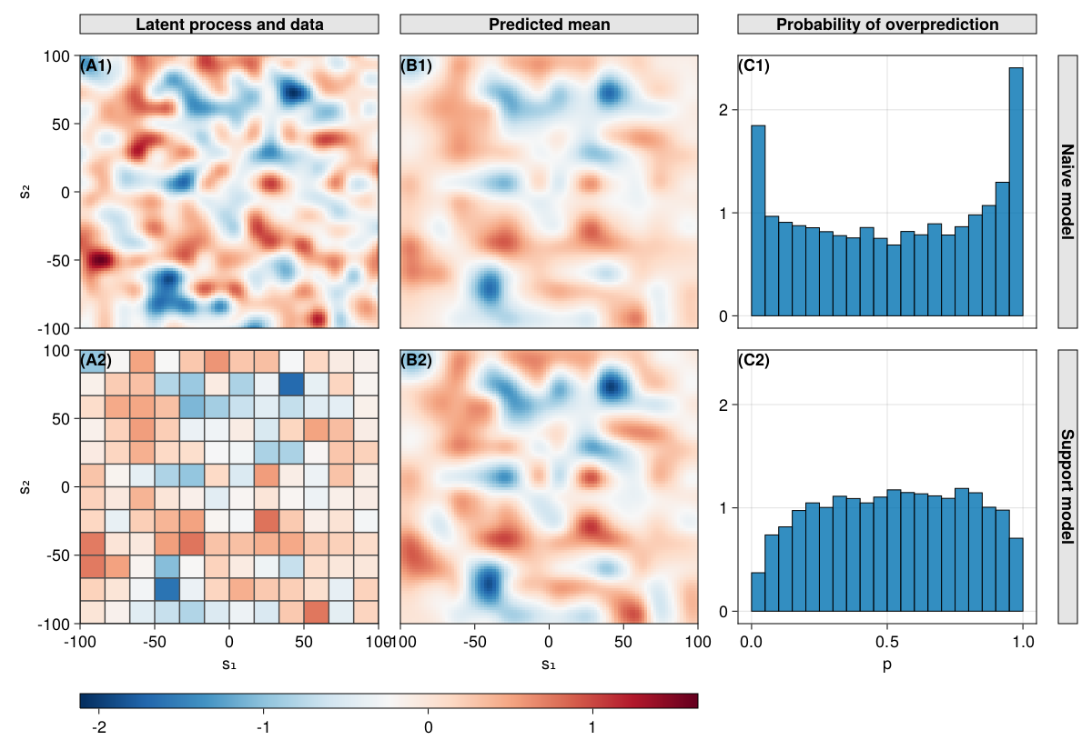
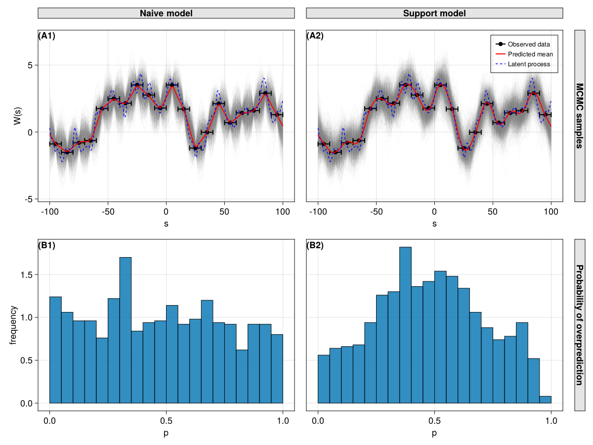
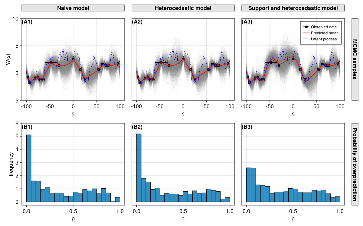
Bayesian inference is carried out through Gibbs sampling. In all of our experiments, we generated 10,000 MCMC samples, removed the first 2,000 samples, and retained every 1 out of 5 samples. Subsequently, the continuous latent process is predicted using the MCMC samples and the basis functions associated with the sampling units. The models are compared by analysing the characteristics of the predicted mean function, the uncertainty associated with the prediction, and their posterior probability of overpredicting the true process at locations within the study area, defined as:
| (8) |
4.1.1 Regular grid
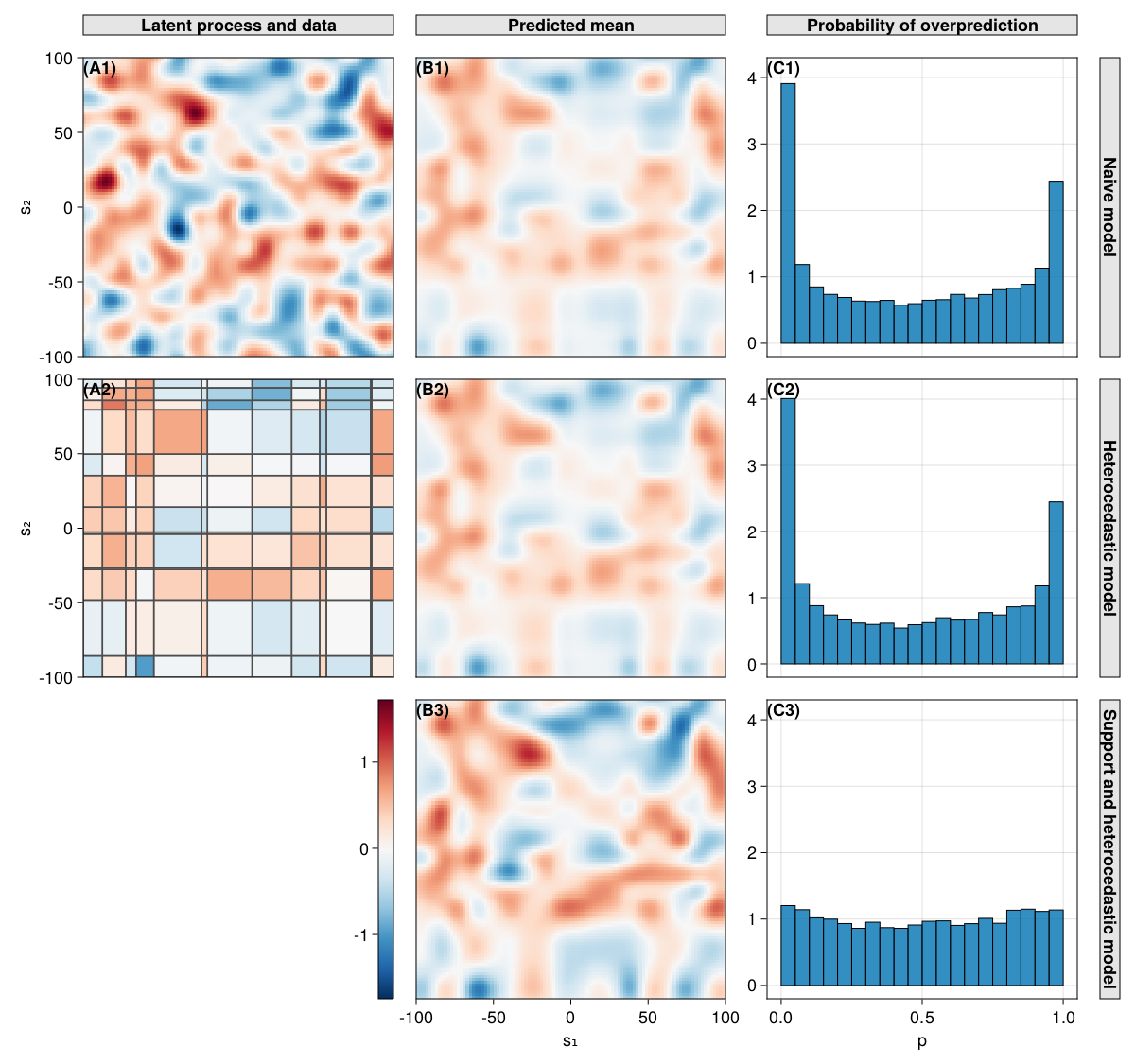
For this experiment, we define the latent process using 400 basis functions of degree 2 and a GMRF of order 1 with a scale parameter of . Similar to the 1-dimensional case, the support model (M2) outperforms the naive model (M1). Specifically, when examining the predicted mean of M1, it becomes evident that this model tends to underestimate the peaks and overestimate the valleys, resulting in more rapid changes (Figure 2, panels B1-B2). When analysing the posterior probability of overprediction, we observe that M1 exhibits more frequent values close to 1 and 0, indicating a tendency for overprediction and underprediction respectively (Figure 2-C1). Conversely, the support model demonstrates a higher frequency of probabilities of overprediction close to 0.5 (Figure 2-C2). This behaviour is also linked to the fact that the uncertainty tends to be underestimated for locations near the centroids of the sampling units in the naive model.
4.1.2 Irregular grid, sparse sampling units and overlapping sampling units
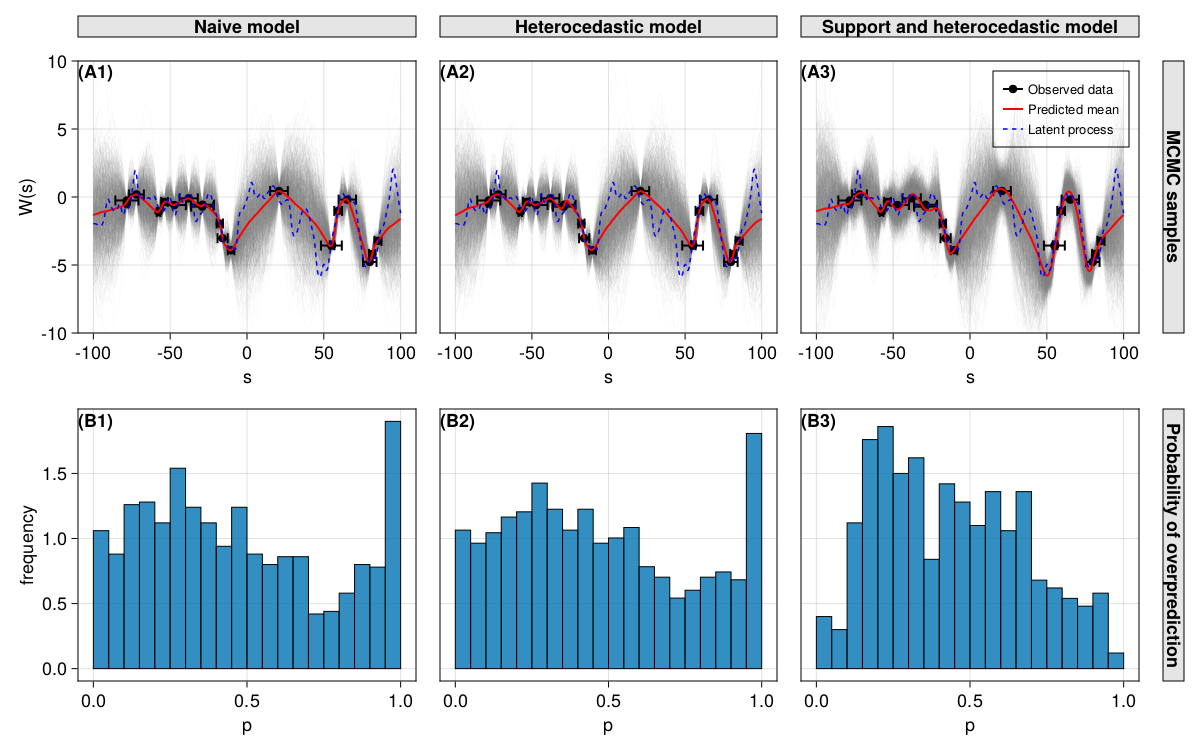
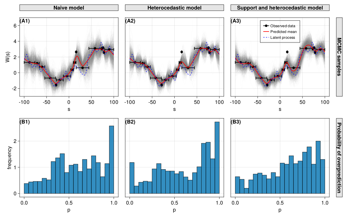
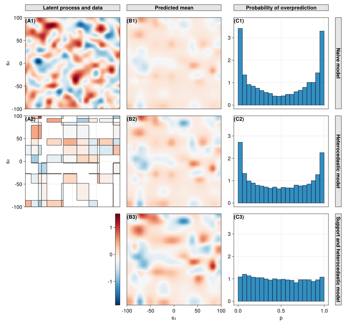
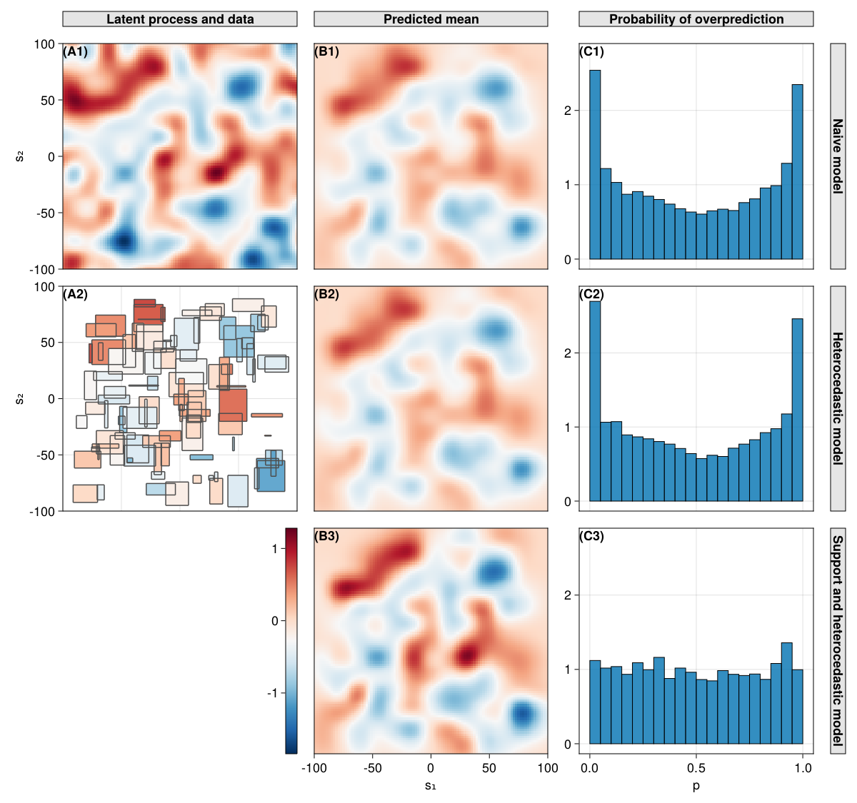
For the irregular grid and sparse sampling units experiments, the latent process was defined with 400 basis functions, while 225 basis functions were used for the experiments with overlapping sampling units. In all three experiments, GMRFs of order 1 with a scale parameter of were employed.
For all three experiments, we consistently observed that both the naive model (M1) and the heteroscedastic model (M2) tend to underestimate the mean function near peaks and overestimate it around valleys, a behaviour reminiscent of what was observed in regular grids (Figure 11, 12, 13 in SM; panels B1-B2). Conversely, the support and heteroscedastic model (M3) consistently yields predicted means closer to the true process values for both peaks and valleys (Figure 11, 12, 13 in SM; panels B3). As a result, the predicted mean range for the support and heteroscedastic model (M3) is generally wider compared to that of M1 and M2. This underestimation and overestimation tendency observed in M1 and M2 is reflected in the posterior probability of overprediction, which shows high-frequency values close to 0 and 1 (Figure 11, 12, 13 in SM; panels C1-C2). In contrast, the support and heteroscedastic model (M3) exhibits significantly lower levels of overprediction and underprediction when compared to M1 and M2 (Figure 11, 12, 13 in SM; panel C3).
A noteworthy attribute of the support and heteroscedastic model (M3) is its proficiency in modelling data acquired under various sampling unit configurations. It captures essential properties of the underlying process and provides a suitable uncertainty quantification, even with sparse and overlapping sampling units. This underscores the effectiveness of the model in predicting the continuous latent process when data are observed on aggregated units.
4.2 Multiple binary data and aggregated predictors
In this section, we present a more realistic scenario involving binary response data observed by two instruments, where the second includes a bias. Predictors are observed at two different aggregated resolutions. The objective is to recover the parameters of the system and perform predictions of the latent processes.
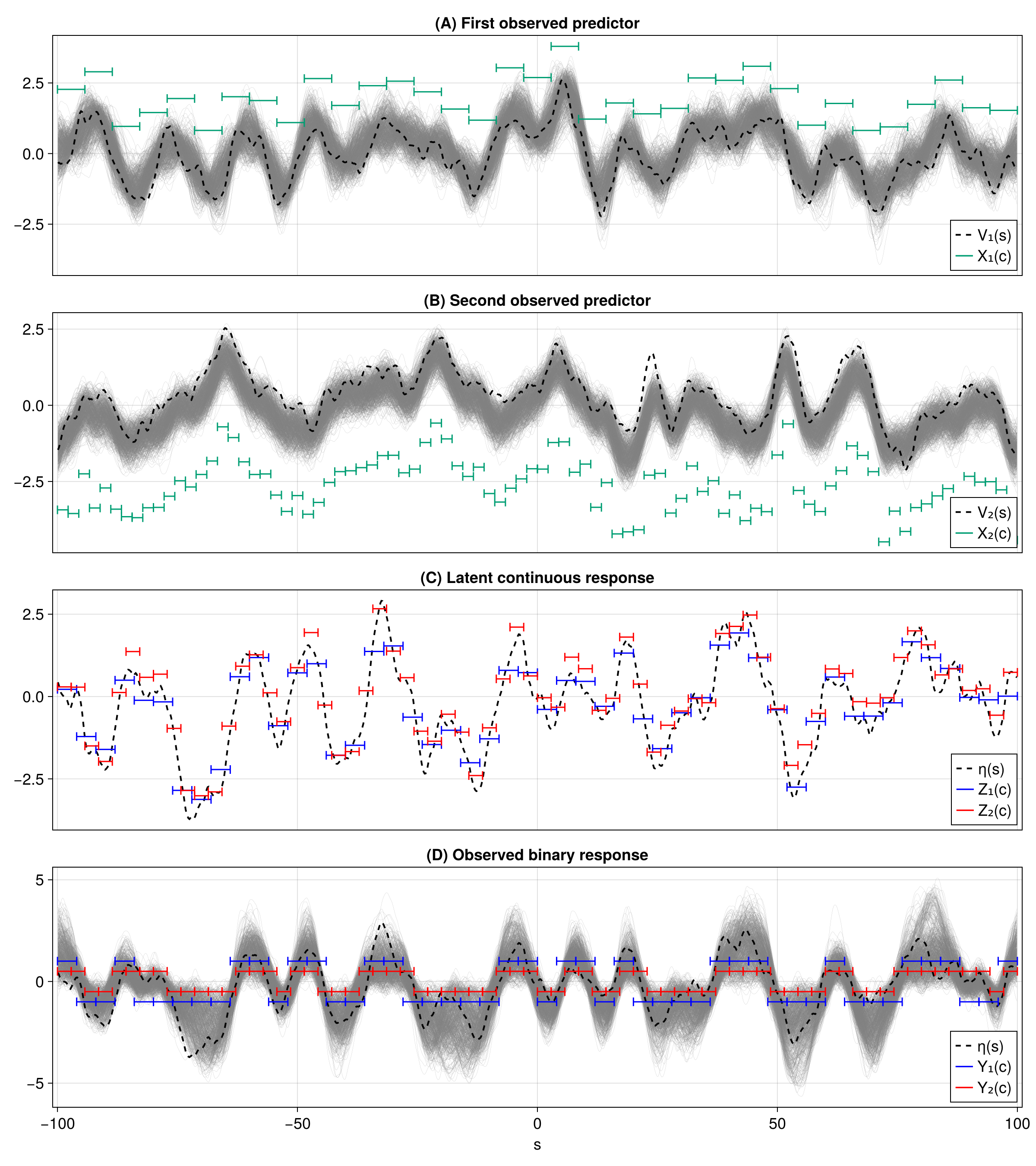
Panels (A) and (B) in Figure 3 depict the latent processes and along with observations at regular sampling units with lengths of and , respectively. Panel (C) presents the latent process , with noisy values having unit lengths of and , respectively. It is important to note that the second source includes a bias of . Finally, Panel (D) shows the binary observations from the two sources at resolutions and , respectively. These observations are simply a binarisation around of the noisy values shown in Panel (C).
We conducted Bayesian inference with the aggregated predictors and binary aggregated outcomes for the change of support model, as outlined in Section 3.2.3, using the Gibbs sampling algorithm explained in Section C.2.2. The algorithm was executed with 10,000 iterations, discarding the initial 2,000 iterations and retaining every 10th iteration. In Panels (A), (B), and (D) of Figure 3, the predictive samples of the latent processes are shown as grey solid lines.
For the first predictor (Panel A), the predictive samples effectively capture the pattern of the latent process, and the uncertainty bounds appropriately cover the latent process. Regarding the second predictor (Panel B), the predictive samples also capture the patterns of the latent process, exhibit a realistic uncertainty, and show a small mean bias. This bias is being accounted for by the intercept parameter . The key results are observed in Panel (D), where the predictive samples of the latent process accurately capture its patterns. Importantly, these predictions from binary aggregated outcomes and aggregated predictors do not exhibit the problems of approaches that disregard the support discussed in previous sections. Additionally, the mean bias in the latent predictor does not introduce bias in the prediction of the main process of interest , as it is effectively compensated by the intercept parameter in the response variable.
5 Land suitability modelling in Rhondda Cynon Taf
Land suitability refers to the appropriateness of a piece of land for a specific use or purpose (Jafari and Zaredar,, 2010). This concept is crucial in land use planning, resource management, and environmental conservation. While land suitability itself is not directly observable, it can be inferred through the examination of climatic, internal soil and external soil characteristics (Wang,, 1994). In this section, we employ land cover data and predictors at various resolutions to predict land suitability for improved grassland in Rhondda Cynon Taf, a county borough in Wales. The resulting predictions can be used for further analysis, as demonstrated, for example, in Brown et al., (2022), where land suitability surfaces are used as input to generate future scenarios in the British land use system.
5.1 Data description
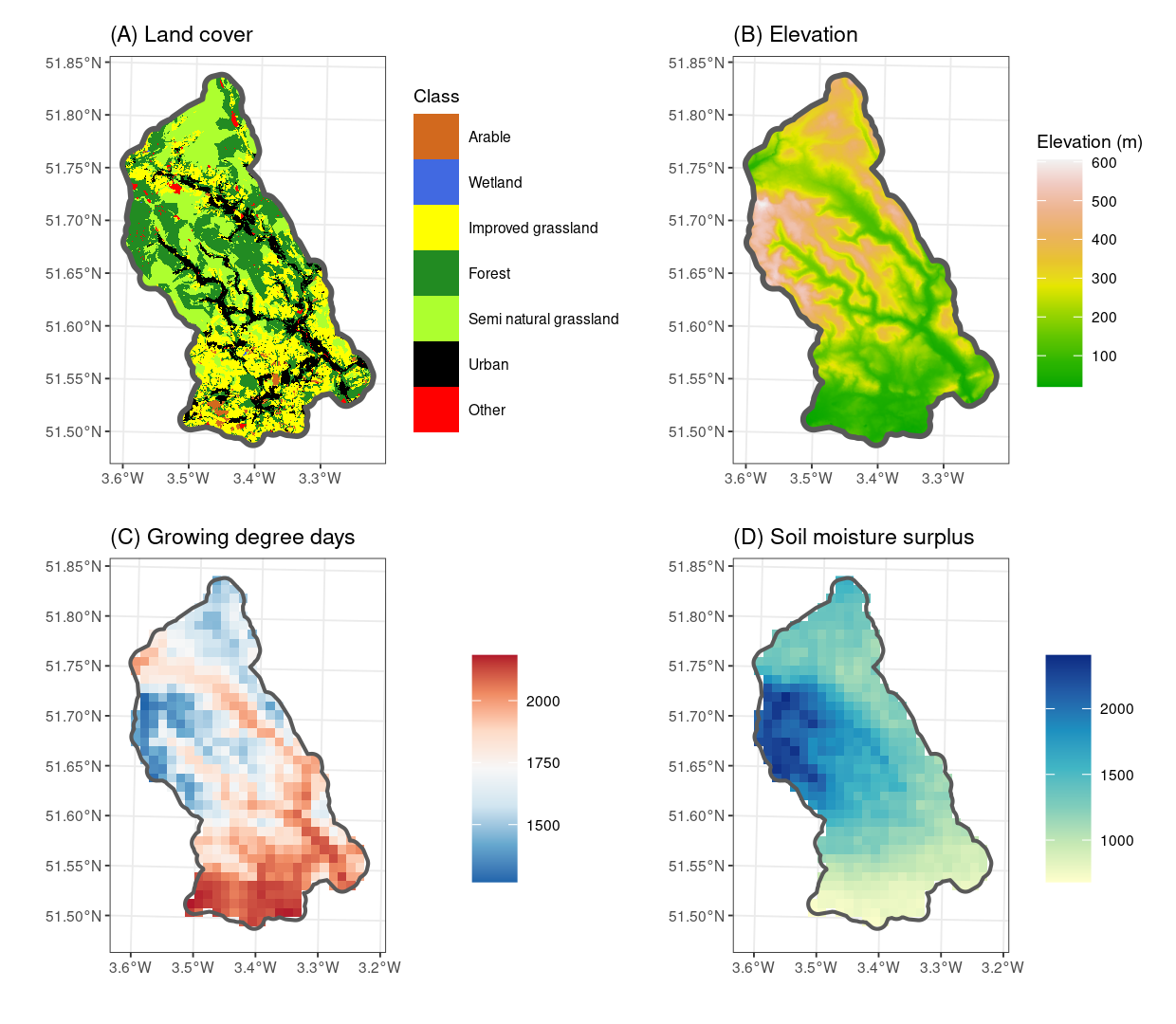
The data employed in our land suitability modelling is depicted in Figure 4. In Panel (A), we showcase the land cover data extracted from the 2017 UK land cover map at a resolution, comprising cells for our selected study area (Morton et al.,, 2020). This dataset is provided by the UK Centre for Ecology and Hydrology (UKCEH) and can be accessed at https://www.ceh.ac.uk/data/ukceh-land-cover-maps. Moving to Panel (B), we present elevation data at a resolution comprising cells, supplied by Copernicus and available at https://spacedata.copernicus.eu/collections/copernicus-digital-elevation-model. It is important to note that, despite both datasets having a resolution of , their support does not align.
Panels (C-D) in Figure 4 depict growing degree days (GDD) and soil moisture surplus (SMS) at resolution comprising cells. These variables play a significant role in determining land suitability and are available as annual means for a period of 20 years (1991-2011) describing the general characteristics of the land. While air temperature variables (maximum, minimum, and mean) and soil moisture deficit (SMD) are also available, the former ones exhibit high correlation with growing degree days (), and the latter is zero constant across the extent of Rhondda Cynon Taf; consequently, they were not included in our analysis. For detailed information on the computation of growing degree days refer to Robinson et al., (2017); Robinson et al., 2023a . Soil moisture was computed using the method outlined by Cosby et al., (1984), incorporating evapotranspiration, precipitation, and available water content (Robinson et al., 2023b, ; FAO/IIASA/ISRIC/ISS-CAS/JRC,, 2012).
5.2 Modelling with change of support
Consider as the land class of interest at cell , and as predictor at cell of the data source (). The observation model defines land cover as a binarisation of a latent process which depends on a spatial process and an error term , and it defines the predictors in terms of latent processes and an error term .
Note that and capture that main spatial patterns presented in land cover and the predictor , respectively. These processes are related to continuous processes in the change of support model such as
The relationship between the continuous latent processes of interest is defined in the latent model. Considering as the land suitability at location , then we define This implies that land suitability depends on the observed predictors through and influences land cover through . In this model, one of our primary interests is to predict the latent continuous process that defines land cover . However, more importantly, we aim to predict the latent land suitability at different supports while considering the associated uncertainty.
5.3 Results
Urban areas were masked out to avoid assuming that land suitability determined by the current urban status. This decision aligns with our objective to characterize land suitability based on climatic, internal soil, and external soil characteristics, aiming to capture the variability that influences land suitability beyond the presence of urban development. We did not include elevation as it was strongly correlated with GDD. The results described below are based on the model of Section 5.2 including GDD and SMS as predictors.
5.3.1 Inference
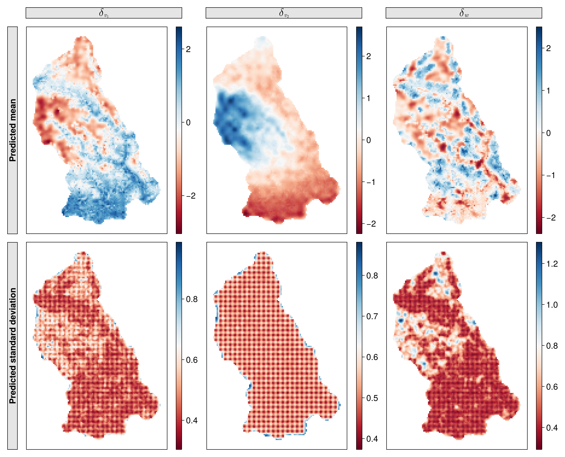
Figure 16 of SM illustrates the inference of the latent processes in the model. It can be observed that the mean of the latent process captures the patterns observed in growing degree days (Figure 4-C), while the mean of captures the patterns observed in soil moisture (Figure 4-D). The additional spatial variation not explained by either of the latent predictors is captured by . On the bottom panels, we can also observe the uncertainty associated with these latent processes, with similar patterns for the uncertainty of GDD and SMS. The estimated credible interval for the intercept is , related to the global proportion of observed cells with improved grassland. The latent predictor with respect to growing degree days has a positive effect (CI: ) in defining the chance of a cell being improved grassland, while the latent predictor related to soil moisture surplus has also a positive effect (CI: ).
5.3.2 Prediction
Our model can provide predictions at different resolutions, considering the properties associated with changes in support. The prediction of the latent land cover at 100m, 500m, and 1km can be observed in Figure 5. All predictions capture the main patterns observed in the distribution of improved grassland (Figure 4-A). Particularly, it can be seen that north and west areas have lower levels of improved grassland, and uncertainty is higher in those areas. High levels of latent land cover are predicted even in areas where urban zones are present because we could easily mask out the urban cells and remove their influence. This task is not trivial if land-cover data is aggregated. Additionally, the standard deviation of predictions becomes smaller as we reduce the resolution of the process.

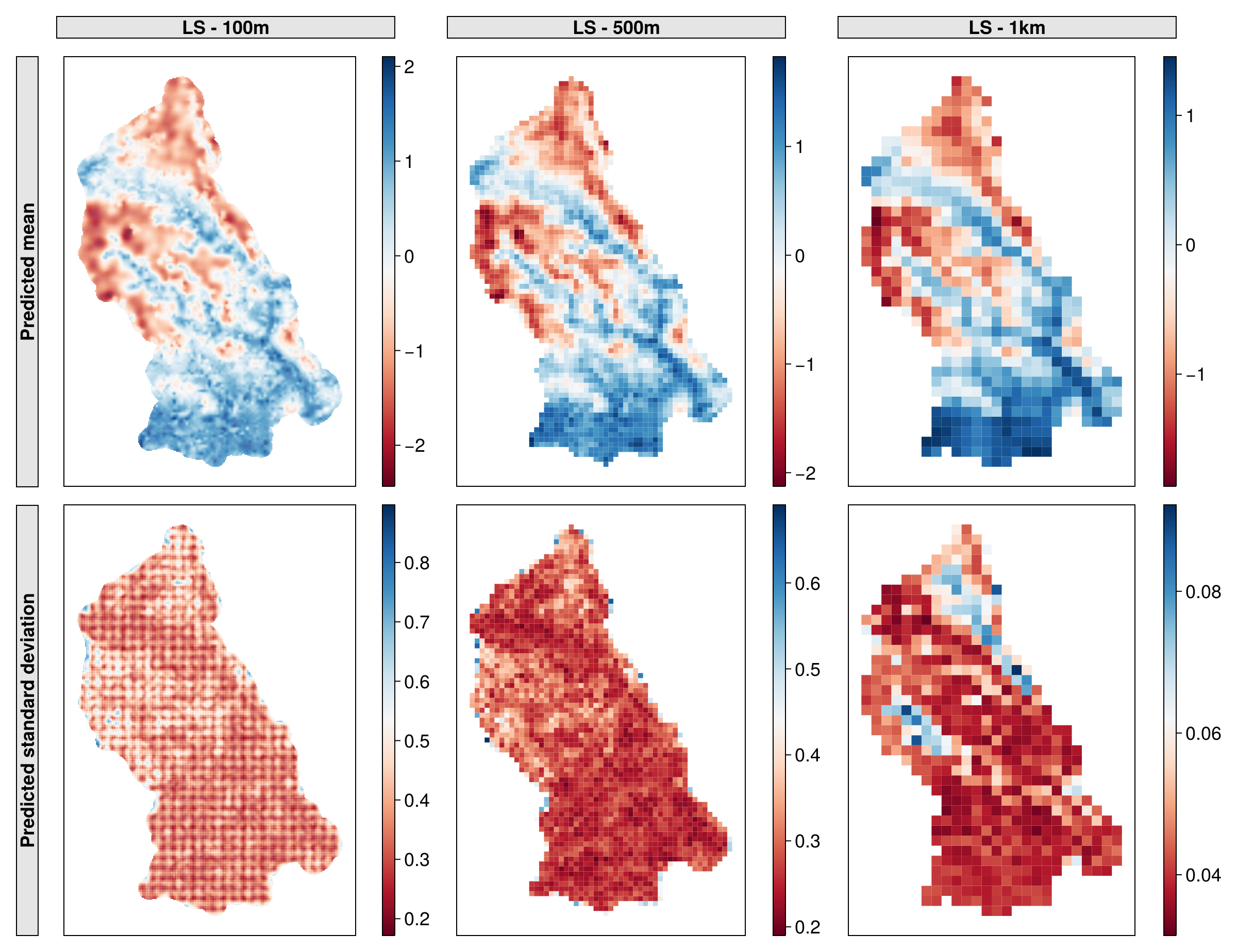
Although our model can predict the latent land cover, our primary goal is to predict land suitability, interpreted as the variability explained by intrinsic variables. Figure 6 displays the mean and standard deviation of land suitability predictions for improved grassland at 100m, 500m, and 1km resolutions. We observe high levels of suitability in southern areas and low levels are evident in the western regions. Moderately low levels of suitability are found in the north-east. The uncertainty is higher in southern and western areas at different resolutions. Predictions at different resolutions are compatible due to the properties of our approach. These resulting surfaces at the desired resolution can be utilized to predict future scenarios or model land use systems, as demonstrated in Brown et al., (2022).
6 Discussion
We developed an extension of SLGM that can accommodate different spatial rectilinear supports for both response and predictor data sources. Our approach consists of three main components: the latent Gaussian model defining system relationships at a continuous level, the change of support model projecting latent processes to other supports, and the observation model describing data generation mechanisms while acknowledging possible mean biases between data sources and heteroscedasticity in measurement errors.
In this framework, employing a spatial process with a closed form to efficiently handle projection to other supports is crucial. We proposed the use of a linear combination of Gaussian Markov random fields (GMRF) and basis splines, ensuring that the projection to other supports depends only on the GMRF and the integral of basis splines over geometries of interest. This approach provides computational advantages, as the projection does not need approximations on rectilinear grids. The transparent relationship between the continuous process and the aggregated process is facilitated through the defined GMRF. The model is computationally efficient, leveraging the sparse properties of GMRFs and basis splines, enabling inference and prediction with change of support for large datasets.
Through data simulation, we assessed the efficacy of our model in one and two-dimensional spaces, considering regular grids, irregular grids, sparse sampling units, and overlapping sampling units. Consistently, we observed that models neglecting the support introduce biases in mean and uncertainty quantification and are more prone to over and underprediction. Conversely, our model captures the main trends of the underlying processes, providing reliable estimates of uncertainty and exhibiting low levels of over and underprediction. We further evaluated the adequacy of our model on a more complex simulated dataset with binary outcomes, different supports for two data sources, and predictors observed at varying resolutions. Our model not only provided predictions about the latent processes but also recovered patterns in the latent response process with reliable uncertainty quantification.
Furthermore, we demonstrated the applicability of our approach in modeling land cover at a 25m resolution in Rhondda Cynon Taf (Wales), utilizing elevation (25m), growing degree days (1km), and soil moisture surplus (1km). Our model predicted spatial latent processes behind these variables and provided predictions of latent land cover and land suitability for improved grassland at various resolutions (100m, 250m, and 1km) along with associated uncertainties. Our results improved upon previous analyses conducted at a 1km resolution, addressing differences in support and computational challenges.
Future avenues involve approximating the change of support onto irregular geometries using a quadtree representation or efficient Monte Carlo integration. Additionally, we aim to extend this work to spatial point processes, and model jointly with aggregated count data. This requires establishing an appropriate relationship between aggregated and continuous processes in under transformations of latent processes. Efficient sampling algorithms for the full model are also required due to the presence of several latent processes, which can be achieved by marginalizing some of the latent processes.
References
- Alegana et al., (2016) Alegana, V. A., Atkinson, P. M., Lourenço, C., Ruktanonchai, N. W., Bosco, C., zu Erbach-Schoenberg, E., Didier, B., Pindolia, D., Le Menach, A., Katokele, S., Uusiku, P., and Tatem, A. J. (2016). Advances in mapping malaria for elimination: Fine resolution modelling of Plasmodium falciparum incidence. Scientific Reports, 6.
- Bradley et al., (2016) Bradley, J. R., Wikle, C. K., and Holan, S. H. (2016). Bayesian Spatial Change of Support for Count-Valued Survey Data With Application to the American Community Survey. Journal of the American Statistical Association, 111(514):472–487.
- Brown et al., (2022) Brown, C., Seo, B., Alexander, P., Burton, V., Chacón-Montalván, E., Dunford, R., Merkle, M., Harrison, P., Prestele, R., Robinson, E. L., et al. (2022). Agent-based modeling of alternative futures in the british land use system. Earth’s Future, 10(11):e2022EF002905.
- Cosby et al., (1984) Cosby, B., Hornberger, G., Clapp, R., and Ginn, T. (1984). A statistical exploration of the relationships of soil moisture characteristics to the physical properties of soils. Water resources research, 20(6):682–690.
- Cowles et al., (2009) Cowles, M. K., Yan, J., and Smith, B. (2009). Reparameterized and Marginalized Posterior and Predictive Sampling for Complex Bayesian Geostatistical Models. Journal of Computational and Graphical Statistics, 18(2):262–282.
- de Boor, (2001) de Boor, C. (2001). A Practical Guide to Splines. Springer New York.
- Diggle and Ribeiro, (2007) Diggle, P. and Ribeiro, P. J. (2007). Model-Based Geostatistics. Springer.
- Dungan et al., (2002) Dungan, J. L., Perry, J. N., Dale, M. R., Legendre, P., Citron-Pousty, S., Fortin, M. J., Jakomulska, A., Miriti, M., and Rosenberg, M. S. (2002). A balanced view of scale in spatial statistical analysis. Ecography, 25(5):626–640.
- FAO/IIASA/ISRIC/ISS-CAS/JRC, (2012) FAO/IIASA/ISRIC/ISS-CAS/JRC (2012). Harmonized world soil database (version 1.2).
- Finley et al., (2014) Finley, A. O., Banerjee, S., and Cook, B. D. (2014). Bayesian hierarchical models for spatially misaligned data in R. Methods in Ecology and Evolution, 5(6):514–523.
- Gelfand et al., (2001) Gelfand, A. E., Zhu, L., and Carlin, B. P. (2001). On the change of support problem for spatio-temporal data. Biostatistics, 2(1):31–45.
- Gotway and Young, (2002) Gotway, C. A. and Young, L. J. (2002). Combining Incompatible Spatial Data. Journal of the American Statistical Association, 97(458):632–648.
- Jafari and Zaredar, (2010) Jafari, S. and Zaredar, N. (2010). Land suitability analysis using multi attributedecision making approach. International journal of environmental science and development, 1(5):441.
- Kyriakidis, (2004) Kyriakidis, P. C. (2004). A Geostatistical Framework for Area-to-Point Spatial Interpolation. Geographical Analysis, 36(3):259–289.
- Law et al., (2018) Law, H. C., Sejdinovic, D., Cameron, E., Lucas, T., Flaxman, S., Battle, K., and Fukumizu, K. (2018). Variational Learning on Aggregate Outputs with Gaussian Processes. In Advances in Neural Information Processing Systems, volume 31. Curran Associates, Inc.
- Lee and Anderson, (2022) Lee, D. and Anderson, C. (2022). Delivering spatially comparable inference on the risks of multiple severities of respiratory disease from spatially misaligned disease count data. Biometrics, n/a(n/a).
- Leopold et al., (2006) Leopold, U., Heuvelink, G. B. M., Tiktak, A., Finke, P. A., and Schoumans, O. (2006). Accounting for change of support in spatial accuracy assessment of modelled soil mineral phosphorous concentration. Geoderma, 130(3):368–386.
- Lindgren et al., (2011) Lindgren, F., Rue, H., and Lindström, J. (2011). An explicit link between gaussian fields and gaussian markov random fields: The stochastic partial differential equation approach. Journal of the Royal Statistical Society. Series B: Statistical Methodology, 73(4):423–498.
- Ma and Kang, (2020) Ma, P. and Kang, E. L. (2020). Spatio-Temporal data fusion for massive sea surface temperature data from MODIS and AMSR-E instruments. Environmetrics, 31(2):e2594.
- Moraga et al., (2017) Moraga, P., Cramb, S. M., Mengersen, K. L., and Pagano, M. (2017). A geostatistical model for combined analysis of point-level and area-level data using INLA and SPDE. Spatial Statistics, 21:27–41.
- Morton et al., (2020) Morton, R., Marston, C., O’Neil, A., and Rowland, C. (2020). Land cover map 2017 (25m rasterised land parcels, gb).
- Pacifici et al., (2019) Pacifici, K., Reich, B. J., Miller, D. A. W., and Pease, B. S. (2019). Resolving misaligned spatial data with integrated species distribution models. Ecology, 100(6):e02709.
- Rasmussen and Williams, (2005) Rasmussen, C. E. and Williams, C. K. I. (2005). Gaussian Processes for Machine Learning. MIT Press.
- Reich et al., (2014) Reich, B. J., Chang, H. H., and Foley, K. M. (2014). A spectral method for spatial downscaling. Biometrics, 70(4):932–942.
- (25) Robinson, E., Blyth, E., Clark, D., Comyn-Platt, E., Finch, J., and Rudd, A. (2023a). Climate hydrology and ecology research support system meteorology dataset for great britain (1961-2019)[chess-met].
- (26) Robinson, E., Blyth, E., Clark, D., Comyn-Platt, E., Rudd, A., and Wiggins, M. (2023b). Climate hydrology and ecology research support system potential evapotranspiration dataset for great britain (1961-2019)[chess-pe].
- Robinson et al., (2017) Robinson, E. L., Blyth, E. M., Clark, D. B., Finch, J., and Rudd, A. C. (2017). Trends in atmospheric evaporative demand in great britain using high-resolution meteorological data. Hydrology and Earth System Sciences, 21(2):1189–1224.
- Rue and Held, (2005) Rue, H. and Held, L. (2005). Gaussian Markov Random Fields: Theory and Applications. CRC Press.
- Taylor et al., (2018) Taylor, B. M., Andrade-Pacheco, R., and Sturrock, H. J. W. (2018). Continuous inference for aggregated point process data. Journal of the Royal Statistical Society. Series A (Statistics in Society), 181(4):1125–1150.
- Taylor et al., (2015) Taylor, B. M., Davies, T. M., Rowlingson, B. S., and Diggle, P. J. (2015). Bayesian Inference and Data Augmentation Schemes for Spatial, Spatiotemporal and Multivariate Log-Gaussian Cox Processes in R. Journal of Statistical Software, 63(7):1–48.
- Wang et al., (2018) Wang, C., Puhan, M. A., and Furrer, R. (2018). Generalized spatial fusion model framework for joint analysis of point and areal data. Spatial Statistics, 23:72–90.
- Wang, (1994) Wang, F. (1994). The use of artificial neural networks in a geographical information system for agricultural land-suitability assessment. Environment and planning A, 26(2):265–284.
- Young et al., (2009) Young, L. J., Gotway, C. A., Kearney, G., and DuClos, C. (2009). Assessing Uncertainty in Support-Adjusted Spatial Misalignment Problems. Communications in Statistics - Theory and Methods, 38(16-17):3249–3264.
- Zhu et al., (2003) Zhu, L., Carlin, B. P., and Gelfand, A. E. (2003). Hierarchical regression with misaligned spatial data: Relating ambient ozone and pediatric asthma ER visits in Atlanta. Environmetrics, 14(5):537–557.
In this supplementary material, we delve into theoretical insights and proofs regarding the integral of basis splines in Section A. We then explore common spatial stochastic processes utilized in spatial latent Gaussian models (SLGM) in Section B. Additionally, we discuss the theory of SLGM with change of support in Section C, covering Bayesian inference and spatial prediction. Further details on simulation studies are provided in Section D. The MCMC algorithm chains for our case study are showcased in Section E. Lastly, spatial prediction of the latent processes for land suitability is presented in Section F.
Appendix A Basis splines
A.1 Introduction
Definition 1.
Let be a strictly increasing break sequence, and represent homogeneous conditions. Then, is defined as the space of piecewise -th order polynomial functions.
A function belonging to the space is characterized by -order polynomials from to and satisfies homogeneous conditions, specifically for and . As an example, when and , this space is associated with natural cubic splines.
Basis splines or B-splines, defined over a non-decreasing sequence of knots , serve as efficient basis functions for the space of piecewise polynomial functions (de Boor,, 2001). The knots are determined by and in such a way that occurs times in . Note that in the case of natural cubic splines, the breaks occur only once in .
Definition 2.
Considering a non-decreasing sequence of knots , the -th basis spline of order is defined as
which is equal to
The operator represents the k-th divided difference of the function , which is defined as the leading coefficient of the order polynomial function that agrees with at knots . Additionally, represents the truncated function of at . While the above definition is useful for proving properties of basis splines, for implementation, it is better to use the following representation.
Theorem 1.
Let be a non-decreasing sequence. The basis splines of order 1 are given by
Additionally, the basis splines of order can be recursively expressed as
where .
The basis spline of order one is directly derived from Definition 2, and the recursive relationship is established by applying the properties of the -th divided difference (de Boor,, 2001).
Definition 3.
A spline function of order belonging to the space and corresponding knot sequence is defined as a linear combination of basis splines,
where is build with respect to the knot sequence .
Out interest in to use spline functions to represent latent processes using stochastic weights . In the following sections, we analyse the differentiation and integration of basis splines and spline functions.
A.2 Differentiation
Theorem 2.
Let be a basis spline of order starting at knot . Then, the derivative can be expressed with respect to the basis splines of order as follows:
Proof.
Corollary 1.
Let be a spline function of order and corresponding knot sequence with coefficients when , then the derivative of is
Proof.
| (by Theorem 2) | ||||
The last equality holds because and . ∎
A.3 Integration
Theorem 3.
Let be a basis spline of order starting at knot . Then, the integral for can be expressed with respect to the basis splines of order as follows:
where .
Proof.
Given that the basis spline is non-zero from to , then we can evaluate the integral from to an arbitrary value . Using Theorem 2 to the basis function , we obtain that
Replacing using the above equivalence, then
For such as . The previous result holds because for . ∎
Corollary 2.
Let be a basis spline of order starting at knot . Then, the integral for and can be expressed with respect to the basis splines of order as follows:
where .
Proof.
Corollary 3.
Let be a spline function of order and corresponding knot sequence with coefficients when , then the integral of is
where .
Proof.
Appendix B Spatial latent Gaussian models
B.1 Spatial Stochastic Processes
Spatial stochastic processes are essential for the definition of SLGMs. In this section, we provide more information about Gaussian processes, Gaussian Markov random fields, and linear transformations of basis functions which are essential stochastic processes for spatial modelling.
B.1.1 Gaussian Processes
A spatial Gaussian process (GP) is a stochastic process with a continuous index set. It is characterised by the property that any finite subset of random variables follows a multivariate Gaussian distribution (Rasmussen and Williams,, 2005; Diggle and Ribeiro,, 2007). The process is defined by a mean function and a covariance function, also known as a kernel function, denoted as for any pair of locations . Gaussian processes are widely utilised for modelling spatial data due to their ability to model dependencies using kernel functions, facilitate statistical inference (both classical and Bayesian), and provide predictions with uncertainty quantification which is crucial for decision-making.
B.1.2 Gaussian Markov Random Fields
A spatial Gaussian Markov random field (GMRF) is a stochastic process with a discrete index set where each represents a non-overlapping region. Let the connectivity of the index set be defined by the undirected graph with nodes and edges . Then, the random vector follows a multivariate Gaussian distribution with mean and precision matrix such as
| (9) |
In cases where is a semidefinite matrix with rank , the process is known as an intrinsic Gaussian Markov random field (IGMRF) with density
| (10) |
where denotes the generalised determinant (Rue and Held,, 2005). The precision matrix can usually be decomposed as the product of a scalar precision parameter and a structure matrix .
Gaussian Markov random fields are used because they capture the spatial structure based on the connectivity of the index elements, resulting in a sparse precision matrix . This sparsity leads to lower computational costs compared to Gaussian processes. The applicability of GMRF is limited to discrete index sets. However, they can also be used to represent Gaussian processes through their connection with stochastic partial differential equations (Lindgren et al.,, 2011).
B.1.3 Linear Combinations of Spatial Basis Functions
Another type of continuous-index spatial stochastic process can be obtained as a linear combination of spatial basis functions such as Where , for , are the weights associated to the basis functions. In particular, we focus on the case where the basis functions are locally defined and the spatial structure is introduced by defining as a GMRF with a two-dimensional regular grid as an index set. More specifically, consider the regular grid with and knots corresponding to basis splines and of order for the first and second coordinates, respectively. Then, the spatial process can be written as
| (11) |
where is a -dimensional GMRF and is a vector containing the two-dimensional basis functions expressed as the tensor product of two sets of one-dimensional basis splines of order . The advantage of using locally defined basis functions and GMRF is that has also sparse properties leading to lower computational costs.
Appendix C Spatial latent Gaussian model with change of support
C.1 Change of Support on Stochastic Processes
C.1.1 Gaussian Processes
Inference:
Using the properties of a GP for change of support, we can express the likelihood function for observations with sampling units as points and/or regions to estimate the parameters defined in the mean function and the covariance function . However, it is important to acknowledge that in the most commonly used models, the elements of the covariance matrix cannot be obtained analytically. Therefore, approximation methods, with Monte Carlo integration being the most common, are employed to estimate these quantities at each iteration of the algorithm to obtain the estimates or to obtain samples from the posterior distribution.
Prediction:
Let us consider a setting where we desire predictions at new points and/or regions . Predictions at these new locations, given a set of observations at points and/or regions , follow a multivariate normal distribution with mean vector and covariance matrix
The covariance matrices and are defined as usual, while the cross-covariance matrix is defined as
| (12) |
which depends of the covariance under change of support. Therefore, the predictive distribution at any set of points and/or regions can be derived. However, as in the inference case, approximation methods are required to compute the mean and covariance of the predictive distribution with Monte Carlo integration being the most common.
C.1.2 Linear Combinations of Spatial Basis Functions
Inference:
Consider a set of point-level and region-level observations coming from the following random vectors and . Due to the connection of and through , the conditional joint density of is also a normal distribution with mean and covariance
| (15) |
Given that is also normally distributed, the likelihood associated with the point-level and region-level observations is , where each row of the design matrix is related to the basis functions evaluated at point-level or region-level. Inference is feasible using maximum likelihood or Bayesian inference.
Prediction:
Assuming that we can only observe and through and , respectively, then the predictive distribution at new locations and regions given the realizations at point-level and aggregated-level is
The second term inside the integral is defined by
| (18) |
while the first term is the posterior distribution of , which is a normal distribution with covariance matrix and mean as follows
We obtain realisations of the prediction by sampling from the posterior of and later applying the corresponding linear transformation with Equation 18.
C.2 Bayesian inference and prediction
We introduce the matrix formulation of the spatial latent Gaussian model for binary outcomes under a change of support and subsequently, elucidate a Gibbs sampling scheme to draw samples from the posterior distribution.
C.2.1 Model
Consider as the set of sampling units for the response variable in the th data source for and for as the predictor set. The matrix form of the model for binary outcomes under a change of support can expressed as follows:
Here , and are random vectors of response variables, auxiliary variables and error terms corresponding to the observations for the -th source. Similarly and are the random vectors of predictor variables and error terms corresponding to the observed predictor values . , and are basis functions evaluated at specified location sets, which are associated to the latent processes and . The error terms are assumed to be normally distributed with diagonal covariance matrices such as and . Notice that the auxiliary variables can also be written as where is a design matrix of dummy variables , and is the design matrix of latent predictors for the locations of the -th source, and the set of coefficient parameters.
The Bayesian model is fully specified by imposing a normal prior distribution for , . An inverse-gamma prior distribution for the error variances, such as and . Finally, the scale parameters of the GMRFs are . We do not impose a prior distribution on because it needs to be fixed as explained in Section 3.2.3.
C.2.2 Inference
The posterior distribution of the specified model in the previous section is proportional to:
We can sample from the posterior distribution using Gibbs sampling taking advantage of conjugacy on the conditional posterior distributions. The posterior conditional distributions are presented in Section E of the supplementary material.
For instance, the conditional posterior for the latent random vectors is a truncated multivariate normal distribution:
| (truncated normal) | ||||
On the other hand, the conditional posterior distributions for the latent GMRFs and are multivariate normals. For the former, the posterior uses data available from the response data sources:
| (normal) | ||||
The conditional posterior of uses information from the response data sources but also from the -th predictor:
| (normal) | ||||
The conditional posterior for the regression coefficients is obtained as follows:
| (normal) | ||||
Similarly, the conditional posterior distribution for the intercept coefficients of the predictors are:
| (normal) | ||||
We also take advantage of conjugacy for the error variance parameters , , and the scale parameters . For the response error variances , the conditionals are inverse-gamma distributions:
| (inverse gamma) | ||||
and similarly for the predictor error variances ,
| (inverse gamma) | ||||
Finally, the conditional posteriors for the scale parameters are gamma distributed:
| (gamma) | ||||
C.3 Spatial prediction
Our main interest for spatial prediction is to infer the latent process at new locations (point or geometries). Denoting the associated random vector as with values , the posterior predictive distribution is:
Where the first term on the right-hand side is the marginal posterior distribution for and , while the second term is simply a deterministic relationship: . Samples from the predictive distribution are obtained by taking the samples for and from the posterior and using it to generate samples for with the deterministic expression provided above.
Appendix D Simulation studies
D.1 One dimensional
In the one-dimensional experiments, we used the same scenarios and models explained in Section 4.1. We observe results consistent with the two-dimensional case, with some findings that are more pronounced in 2D due to the larger spatial coverage and increased fluctuations of the simulated latent process. The key findings are summarised in the following sections.
D.1.1 Regular grid
For this experiment, we define using 100 basis functions of degree 2 and a GMRF of order 1 with a scale parameter of . The primary differences observed between the naive model and the support model are described based on the behaviour of the predicted mean, the uncertainty quantification, and their tendency to either overpredict or underpredict the true underlying process.
-
•
Predicted mean: In the naive model (M1), the predicted mean exhibits abrupt changes and tends to overfit the data because it assumes that observations are associated with the centroids of the sampling units (Figure 7-A1). In contrast, the support model (M2) yields a more gradual change in the predicted mean, as it aims to find a function whose integral over the sampling units closely matches the observed data.
-
•
Uncertainty quantification: The naive model (M1) tends to underestimate uncertainty, particularly near the sampling unit centroids (Figure 7-A1). In contrast, the support model (M2) provides more accurate uncertainty estimates, effectively encompassing the true underlying process (Figure 7-A2). These differences stem from the approach of the support model for finding functions whose integrals closely match the data.
-
•
Over and under prediction: The naive model (M1) exhibits more frequent values where the probability of overprediction is close to 1 and close to 0 (indicating underprediction), as seen in Figure 7-B1. In contrast, the support model (M2) features a higher frequency of predictions around the value of 0.5 (Figure 7-B2). This suggests that the support model provides more accurate predictions of the underlying true process.
D.1.2 Irregular grid, sparse sampling units and overlapping sampling units
For the irregular grid experiment, the latent process was defined with 50 basis functions, while 100 basis functions were used for the experiments with sparse and overlapping sampling units. In all three experiments, GMRFs of order 1 with a scale parameter of were employed. The differences between the models observed in Figures 9, 10, and 8 are described below.
Predicted mean:
In the experiment with irregular grids, the naive model (M1) exhibits overfitting similar to the previous experiment with regular grids. It is significantly biased by certain observations due to the lack of accounting for measurement error heteroscedasticity (e.g. for in Figure 9-A1). The heteroscedastic model (M2) performs better by considering observation importance based on support size. In the case of sparse sampling units, both the naive model (M1) and the heteroscedastic model (M2) exhibit abrupt changes in the predicted mean, especially evident in sparse locations like in Figure 10, panels A1-A2. In an attempt to fit the data, these models react strongly to the absence of surrounding information. For overlapping sampling units, the predicted mean of the naive model (M1) and the heteroscedastic model (M2) does not overfit when units are close, but in mixed sparse and overlapping regions, they exhibit abrupt changes and overfitting (e.g. for around in Figure 8, panels A1-A2). Across all three experiments, the support and heteroscedastic model (M3) outperform the naive model (M1) and the heterocedastic model (M2). It yields smoother variation of the predicted mean, avoids overfitting, remains unaffected by high-error observations, and accurately captures primary trends of the underlying true process.
Uncertainty quantification:
In the case of irregular grids, the naive model (M1) tends to overestimate uncertainty because it attempts to increase the variability to capture complex data generation mechanisms. In contrast, the heteroscedastic model (M2) underestimates uncertainty near the sampling unit centroids for sample units of larger size (e.g., in Figure 9-A2). For sparse sampling units, both the naive model (M1) and the heteroscedastic model (M2) tend to underestimate uncertainty for locations near the centroids and locations with sparse data (e.g. in Figure 10, panels A1-A2). In the case of overlapping sampling units, both the naive model (M1) and the heteroscedastic model (M2) tend to underestimate uncertainty for locations near the centroids. For all three experiments, the support and heteroscedastic model (M3) consistently quantifies uncertainty effectively without underestimating it for locations close to the centroids, as observed in M1 and M2, or overestimating it. M3 provides a more accurate quantification of uncertainty, effectively enveloping the underlying true process.
Over and under prediction:
In all the conducted experiments, we observed a higher proportion of posterior probabilities close to 1 or 0 for the naive model (M1) and the heteroscedastic model (M2), as shown in panels B1-B3 of Figures 9, 10, and 8. In contrast, the support and heteroscedastic model (M3) consistently exhibits lower levels of overprediction and underprediction when compared to models M1 and M2, with more frequent probabilities centred around 0.5. This suggests that M3 provides more accurate predictions of the underlying true process.
D.2 Two dimensional
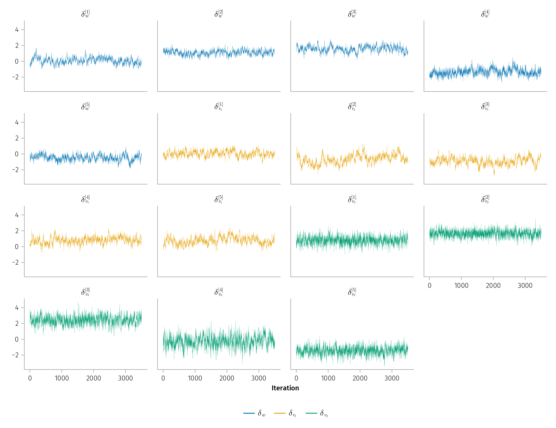
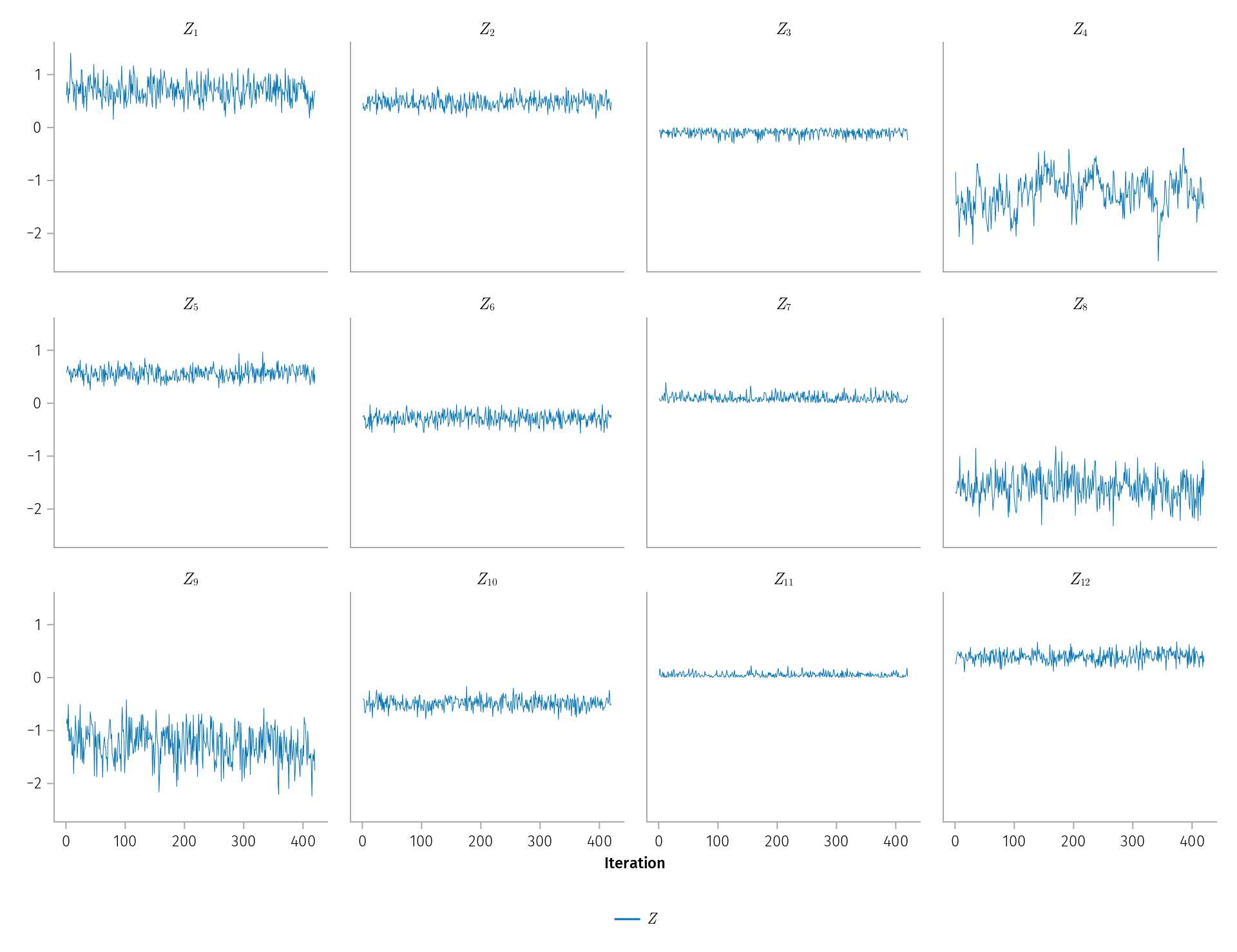
Appendix E MCMC chains
Appendix F Land suitability modelling in Rhondda Cynon Taf