Small field chaos in spin glasses: universal predictions from the ultrametric tree and comparison with numerical simulations.

Abstract

We study the chaotic behavior of the Gibbs state of spin-glasses under the application of an external magnetic field, in the crossover region where the field intensity scales proportional to $1/\sqrt{N}$, being $N$ the system size. We show that Replica Symmetry Breaking (RSB) theory provides universal predictions for chaotic behavior: they depend only on the zero-field overlap probability function $P(q)$ and are independent of other features of the system. Using solely $P(q)$ as input we can analytically predict quantitatively the statistics of the states in a small field. In the infinite volume limit, each spin-glass sample is characterized by an infinite number of states that have a tree-like structure. We generate the corresponding probability distribution through efficient sampling using a representation based on the Bolthausen-Sznitman coalescent. In this way, we can compute quantitatively properties in the presence of a magnetic field in the crossover region, the overlap probability distribution in the presence of a small field and the degree of decorrelation as the field is increased. To test our computations, we have simulated the Bethe lattice spin glass and the 4D Edwards-Anderson model, finding in both cases excellent agreement with the universal predictions.

In low-temperature spin glasses, Replica Symmetry Breaking (RSB) theory predicts that for a given large sample, equilibrium states are non-self-averaging and organized as the leaves of a weighted random tree Mézard et al. (1984a). The statistics of these trees are universal, they depend only on the overlap order parameter function $q(x)$, or equivalently, the average overlap probability distribution $P(q)$. The relative weights of the branches, proportional to the exponential of the free energies of the states, also display universal statistics, obeying the so-called Ruelle probability cascades Ruelle (1987); Mézard et al. (1985); Derrida (1985); Panchenko and Panchenko (2013). Despite having first been derived in the Sherrington-Kirkpatrick (SK) model this structure is completely general, provided that RSB is correct: it is true in more general Mean Field models such as spin glasses on finite coordination random graphs, and even for finite-dimensional spin-glass systems .

This complex statistical structure has striking consequences on the behavior of the overlap distribution function and the magnetization as a function of the external magnetic field $H$ in the crossover region where the magnetic field scales with the system size $N$ as $N^{-1/2}$. We find that these quantities can be exactly computed as a function of $h=HN^{1/2}$ in the infinite volume limit.

Generally speaking, if a system has more than one equilibrium state, the Boltzmann weights of the equilibrium states change when a perturbation is added to the Hamiltonian. This effect is well known, for example, in the Ising ferromagnetic model with symmetric boundary conditions. In this model, the natural Gibbs measure is the mixture of two pure states with positive and negative magnetization $\pm m$ with weights $w_{\pm}=(1\pm\tanh(\beta NHm))/2$, and shows an obvious crossover as a function of $\hat{h}\equiv NH$, and the usual situation with only a single pure state is obtained only for $|\hat{h}|\gg 1$.

The situation is more complex in spin-glasses, where the number of equilibrium states is infinite. When a small random perturbation is added, the Boltzmann weights of the tree’s branches are reshuffled.

As the intensity of the perturbation grows, states that originally had a small weight become dominant, and the overlap between the unperturbed and the perturbed system decreases. For any small but macroscopic perturbation, this implies vanishing similarity, a property known as chaotic dependence on the intensity of the perturbation.

A well-known example of chaotic behavior is chaos against temperature where, however, a variation of temperature does not result in a random perturbation unrelated to the energy landscape (see later). Quantitative predictions are more difficult and less universal: both models with chaos and without chaos are known. Even in mean field models, like the Sherrington-Kirkpatrick model, where chaos is present, explicit computations have only been done near the critical temperature .

In this paper, we study the effect of a magnetic field, where the theory is simpler and chaos has universal features that are absent for temperature chaos . The development of a general theory can be done only because in the absence of a field, the average magnetizations of the states are Gaussian random variables uncorrelated with the energy of the states. This generic property always holds if there are many states and random couplings without a ferromagnetic component.

Remarkably, the predictions of RSB about magnetic field chaos can be submitted to a quantitative test, once the function $P(q)$, or equivalently $q(x)$, at zero magnetic field has been measured. Indeed, one can generate random trees and their relative weights in the absence or the presence of a field, and directly compare with the results of numerical simulations.

In this paper, we compare the theory’s predictions with the simulations of two models exhibiting low-temperature spin glass behavior: the Bethe lattice spin glass and the 4D Edwards-Anderson model. Deviations from the theory can be expected either for finite-size effects or because of the absence of standard RSB. To calibrate the first effect, we study the Bethe lattice spin glass, where the standard RSB structure of the states is present (although only approximate RSB solutions are available); in this case, we find a very good agreement with the theory as expected. In a second moment, we study the 4D spin glass, where qualitatively we find very similar finite size effects. Also, in this case, the agreement is excellent, consistently with clear evidence in favor of RSB in this system at least at zero magnetic field Parisi et al. (1996); Baños et al. (2012); Charbonneau et al. (2023). We are not discussing in this note the existence of RSB in the presence of a fixed non-zero magnetic field where different viewpoints exist (e.g. Ref. Moore (2021)). This issue is not relevant to us because we are working with fields of order $1/N^{1/2}$.

Broken Replica Symmetry theory

For the reader’s convenience, and to establish notations, let us recapitulate the theory using slightly imprecise but simplified language. We suppose to deal with a spin glass without a net ferromagnetic component in the couplings and invariant under spin reversal. In the RSB phase in each instance of the system, there is an infinite number of equilibrium states labeled by $\alpha$. These states have random statistical weights $w_{\alpha}$, normalized to $\sum_{\alpha=1}^{\infty}w_{\alpha}=1$, magnetizations $m_{\alpha}=N^{-1/2}\sum_{i=1}^{N}\langle\sigma_{i}\rangle_{\alpha}$, and mutual overlaps $q_{\alpha\gamma}=N^{-1}\sum_{i=1}^{N}\langle\sigma_{i}\rangle_{\alpha}\langle\sigma_{i}\rangle_{\gamma}$, where $\langle(\cdots)\rangle_{\alpha}$ denotes the statistical average in the state labeled by $\alpha$. The normalization of the magnetization has been chosen to have $m_{\alpha}=O(1)$ for large $N$. In fact, in each state spins freeze in random directions and the $m_{\alpha}$ are Gaussian, zero mean variables, with covariance $\langle m_{\alpha}m_{\gamma}\rangle=q_{\alpha\gamma}$. The positive overlaps are constrained by ultrametricity, implying that the states are organized as random trees, whose statistics we describe later.

It is convenient to define the probability distribution of the overlap for a given disorder realization (sample) $P_{J}(q)$ and its average :

$$P_{J}(q)=\sum_{\alpha,\gamma}w_{\alpha}w_{\gamma}\delta(q-q_{\alpha\gamma})\,,\quad P(q)=\overline{P_{J}(q)}\,,$$ (1)

being $\overline{(\cdots)}$ the average over the disorder. In mean-field models, $P(q)$ has a continuous component and a $\delta$ peak: $P(q)=\tilde{P}(q)+(1-x_{M})\delta(q-q_{\mathrm{EA}})$, with $x(q)=\int_{0}^{q}\mathrm{d}q^{\prime}\,P(q^{\prime})$ and $x(q_{\mathrm{EA}})=x_{M}$. Notice that the function $q(x)$ is defined as the inverse function of $x(q)$.

We can ask now what happens to the overlap when in a given system one replica is at zero magnetic field and the other at non-zero small magnetic field $H=h/\sqrt{N}$ (both replicas of the system share the same disorder). In this regime one only adds a finite perturbation, therefore the states keep their identity, while their weights are modified: $w_{\gamma}\to w_{\gamma}(h)\propto w_{\gamma}\exp(\beta hm_{\gamma})$ with $\sum_{\gamma}w_{\gamma}(h)=1$. Notice that, as it is well known Mézard et al. (1985), the distribution of the weights is left invariant by such a re-weighting independently of the value of $h$. We are interested here to the correlations between the original weights and their re-weighted version. We readily find that the probability distribution of the overlap between the two replicas of the system (one in the absence and the other in presence of the field) is given by

$P_{J,C}(q;h)=\sum_{\alpha,\gamma}w_{\alpha}w_{\gamma}(h)\delta(q-q_{\alpha\gamma})\,,$

or, when both replicas of the system feel the same magnetic field,

$P_{J}(q;h)=\sum_{\alpha,\gamma}w_{\alpha}(h)w_{\gamma}(h)\delta(q-q_{\alpha\gamma})\,.$

An additional grain of salt is due, because the system is invariant under spin reversal at $h=0$. For any state $\alpha$, there is a state $\alpha^{\prime}$ with opposite magnetization and $w_{\alpha^{\prime}}=w_{\alpha}$. It is convenient to remove this degeneracy: we use only one label for each pair of states and we define $q_{\alpha\gamma}$ such that $q_{\alpha\gamma}>0\leavevmode\nobreak\ \forall(\alpha,\gamma)$. This is the convention we use in the generation of the spin glass trees. In the end one reconstructs

$$P^{C}_{J}(|q|;h)=\sum_{\alpha,\gamma}w_{\alpha}w_{\gamma}(h)\delta(q-q_{\alpha,\gamma})\,.$$ (2)

where now $w_{\gamma}(h)\propto w_{\gamma}\cosh(\beta hm_{\gamma})$.

Similarly, the probability distribution of the overlap (positive and negative) between two replicas in a field $P_{J}(\pm|q|;h)$ is:

$$P_{J}(\pm|q|;h)=\sum_{\alpha,\gamma}w_{\alpha}(h)w_{\gamma}(h)g_{\pm}(h,m_{\alpha},m_{\gamma})\delta(|q|-q_{\alpha\gamma})$$ (3)

with $g_{\pm}(h,m_{\alpha},m_{\gamma})=[1\pm\tanh(\beta hm_{\alpha})\tanh(\beta hm_{\gamma})]/{2}$. Remark that in the limit $h\to\infty$ [$H>0$ and $N\to\infty$]: $P_{C}(|q|;\infty)=\delta(q)\,,P(q;\infty)=\theta(q)P(|q|).$

An additional quantity of interest is the average magnetization induced by $h$; using the previous formulae we find that $m(h)=\beta h[1-\int_{-1}^{1}\mathrm{d}q\,qP(q;h)]$ (see SI for details).

Remarkably, all these functions can be computed efficiently, provided that we know the function $P(q)$ at zero magnetic field. The simplest approach, which we follow here, is to average over a large number of random trees generated with the correct statistical properties . The reader may find a detailed explanation of how to generate RSB spin-glass trees of states with the right statistics in Materials and methods. Furthermore, all the technical details of the generation of the trees can be found in the SI.

As explained above, the probability distributions $P(q)$, $P(q;h)$, and $P_{C}(q;h)$ will be the main quantities to study. To compare the theoretical predictions with the simulations, we compute those functions for the Bethe lattice and the 4D Edwards-Anderson model. The details of the computation of the probability distributions $P^{N}(q)$, $P^{N}(q;h)$, and $P^{N}_{C}(q;h)$ for different system sizes $N$ in the simulations can be found in Materials and methods.

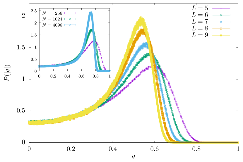
Figure 1: The probability $P^{N}(|q|)$ at $h=0$ for different values of $L$ in 4D EA at $T=0.7\;T_{c}$, $T_{c}(h=0)=2.03(3)$ Marinari and Zuliani (1999). Notice the stable part at low $q$ and the size-dependent peak, whose position shifts to the left, while its height and width respectively increase and decrease as the system size grows. Inset: The probability $P^{N}(|q|)$ at $h=0$ for different values of $N$ in Bethe lattice at $T=0.5\;T_{c}$, with $T_{c}(h=0)\simeq 1.518651$.

The probability distributions $P^{N}(q)$ —as well as $P^{N}(q;h)$ and $P_{C}^{N}(q;h)$— have a strong dependence on $N$ (see Fig. 1), the height of the peak increases (it should go to infinity), and the position of the peak slightly drifts. To minimize finite volume effects, instead of comparing directly the overlap probability distributions, we found it convenient to consider, for $|q|\leq q_{\mathrm{EA}}$, the ratio of the probabilities distributions of the overlaps in the presence and absence of the field

$$R^{N}_{C}(|q|;h)=\frac{P^{N}_{C}(|q|;h)}{P^{N}(|q|;0)}\,,\quad R^{N}(q;h)=\frac{P^{N}(q;h)}{P^{N}(q;0)}\,.$$ (4)

Results

The numerical and theoretical probability distributions are shown in Fig. 2 for the Bethe lattice and in Fig. 3 for the 4D EA model. In both cases, we find an excellent agreement between the theoretical predictions from the ultrametric tree and the numerical results for the functions $P_{C}^{N}(q;h)$ and $P^{N}(q;h)$. We also plot the numerical $P^{N}(q)$, which is used as an input for the theoretical prediction.

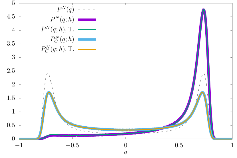
Figure 2: The functions $P^{N}(q)$, $P_{C}^{N}(q;h)$ and $P^{N}(q;h)$ as a function of $q$ at $T=0.5\;T_{c}$ for $h=4$ on Bethe Lattice for the largest volume simulated $N=4096$. We compare both the $P_{C}^{N}(q;h)$ and $P^{N}(q;h)$ curves with the predictions from the ultrametric tree (T.). The dashed line is the zero-field $P^{N}(q)$ function that is the input in our computation. Notice that the probability distributions $P^{N}(q)$, and $P_{C}^{N}(q;h)$ are fully symmetric. Therefore, in the main text, we focus the discussion on $P^{N}(|q|)$, and $P_{C}^{N}(|q|;h)$.

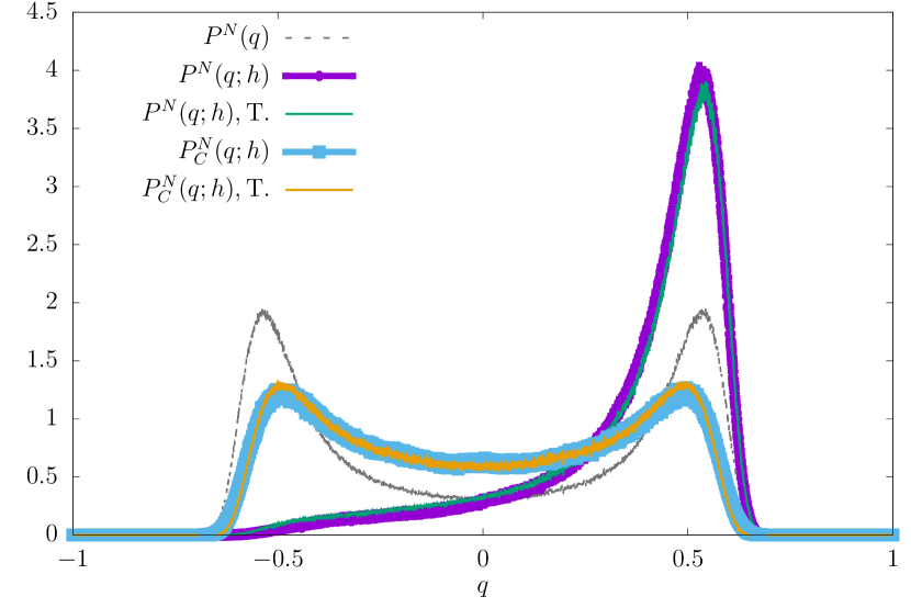
Figure 3: The functions $P^{N}(q)$, $P_{C}^{N}(q;h)$ and $P^{N}(q;h)$ as a function of $q$ at $T=0.7\;T_{c}$ for $h=10$ on the 4D Edwards Anderson for the largest volume simulated $N=9^{4}$. We compare both the $P_{C}^{N}(q;h)$ and $P^{N}(q;h)$ curves with the predictions from the ultrametric tree (T.). The dashed line is the zero-field $P^{N}(q)$ function that is the input in our computation. Notice that the probability distributions $P^{N}(q)$, and $P_{C}^{N}(q;h)$ are fully symmetric. Therefore, in the main text, we focus the discussion on $P^{N}(|q|)$, and $P_{C}^{N}(|q|;h)$.

In these two figures, we show the results for the largest system we have simulated and the reader may be wondering what happens for smaller systems (because the functions $P_{N}(q)$ vary with $N$).

In order to appreciate better the quality of the comparison we find it more convenient to plot the analytic and numerical ratios $R_{C}^{N}(|q|;h)$ and $R^{N}(|q|;h)$. In this way, we can better appreciate the deviations from the theory in the region where the functions $P$’s are small. The detailed results for the function $P_{C}^{N}(|q|;h)$ and for $P^{N}(q;h)$ are shown in the SI.

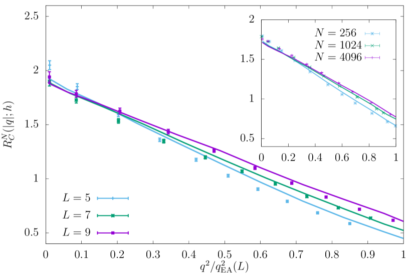
Figure 4: The ratio $R_{C}^{N}(|q|;h)$ as a function of $q^{2}/q_{\mathrm{EA}}^{2}(L)$ at $T=0.7\;T_{c}$ for $h=10$ and different values of $L$ in the 4D EA model. Lines correspond to the theoretical prediction from the ultrametric tree and points correspond to simulations. For visualization purposes, we have plotted only a discrete subset of values of $q$. Inset: Ratio $R_{C}^{N}(|q|;h)$ as a function of $q^{2}/q_{\mathrm{EA}}^{2}(N)$ at $T=0.7\;T_{c}$ for $h=4$ and different values of $N$ in the Bethe lattice.

In Fig. 4 we compare the theoretical predictions for $R_{C}^{N}(|q|;h)$ with the 4D EA computations, and also with the Bethe lattice ones (in the inset). Interestingly, the ratio is a linear function of $q^{2}$ with a good approximation. The plot is done in the region $|q|<q_{\mathrm{EA}}$ where we can directly compare the data with the analytic predictions. The statistical errors increase in the region of small $|q|$ because in that region the probability $P(q)$ is smaller than in the peak.

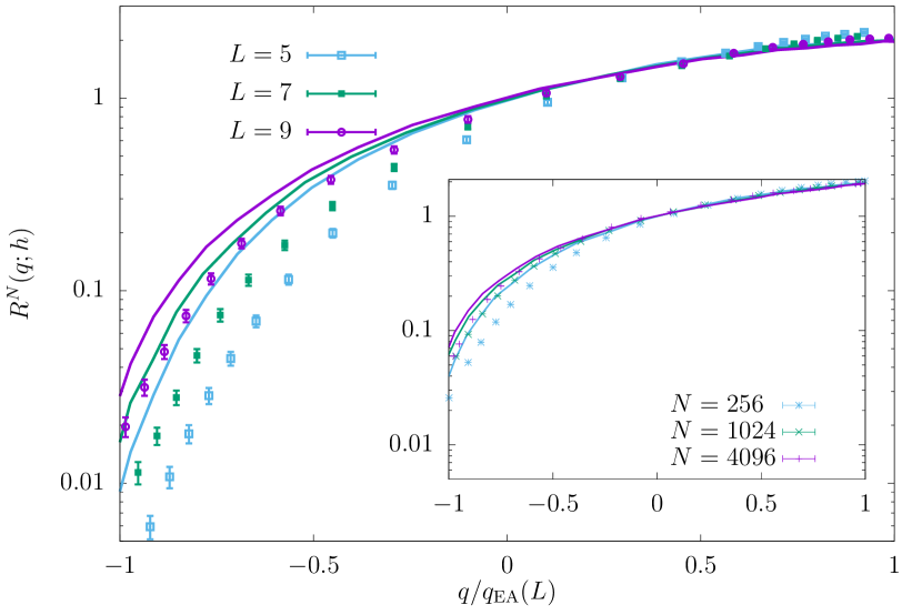
Figure 5: The ratio $R^{N}(q;h)$ as a function of $q/q_{\mathrm{EA}}(L)$ at $T=0.7\;T_{c}$ for different values of $L$ in 4D EA lattice ($h=10$). Lines correspond to the theoretical prediction from the ultrametric tree and points correspond to simulations. For visualization purposes, we have plotted only a discrete subset of values of $q$. Inset: ratio $R^{N}(q;h)$ as a function of $q/q_{\mathrm{EA}}(N)$ at $T=0.5\;T_{c}$ for different values of $N$ in Bethe lattice ($h=4$).

Furthermore, in Fig. 5, we compare the theoretical predictions for $R^{N}(|q|;h)$ with the 4D EA computations and with the Bethe lattice ones (in the inset). Again, the plot is restricted to the region $|q|<q_{\mathrm{EA}}$ where we can directly compare the data with the analytic predictions. The data at negative $q$ have stronger volume dependence. The reasons are quite clear. The theory predicts that this ratio is 1 at $h=0$ because by continuity in $H$ $\mathrm{Prob}(|q|;h)\equiv P(q;h)+P(-q;h)$ is independent of $h$ . On the other hand, for any finite field $H$, the negative values of $q$ should have zero probability in the infinite volume limit. Therefore the region of $q$ near zero (and consequently also for $q<0$) is strongly affected by finite size effects.

We see that for small sizes the analytic computations are less accurate but qualitatively correct: this should be expected as far as the analytic computations are exact only in the infinite volume limit. Moreover, the peaks are wider and the tail of the peaks sometimes arrives near zero: in this situation, our fitting procedure for the function $P(q)$ has a higher degree of approximation. The important message is that the difference between theory and numerical data strongly decreases by increasing the volume.

The asymmetry of the function $P^{N}(q;h)$ is evident: remember that in the limit $h\to\infty$, $P^{N}(q;h)$ for $q<0$ must be zero, and $P^{N}(q;h)=2P^{N}(q)$ for $q\geq 0$, as it happens at an arbitrary small non zero value of $H$ in the infinite volume limit. For finite $h$ the two curves $P^{N}(q;h)$ and $P^{N}(q)$ cross at $q=0$. The chaos effect can be clearly identified as a decrease of the two peaks of $P_{C}^{N}(q;h)$ at $q=\pm q_{\mathrm{EA}}$ and by an increase in the region somewhat far from the peak, in particular in the region of $q$ near zero. Asymptotically, for large $|h|$, $P_{C}^{N}(q;h)$ should become a delta function $\delta(q)$ and we are very far away from this limit.

Finally, an important observable, that could be directly measured in experiments, is the average magnetization as a function of $h$ that verifies:

$$m(h)=\beta h\left(1-\int_{-1}^{1}\mathrm{d}q\;P(q;h)\;q\right)\,.$$ (5)

as shown in the SI. The results are presented in Fig. 6 which displays an excellent agreement between theory and simulations in both our simulated systems.

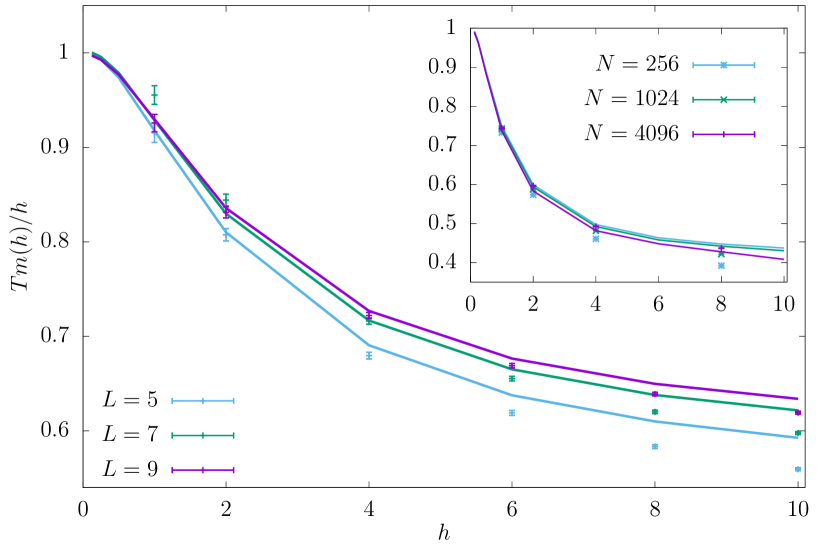
Figure 6: $Tm(h)/h$ as a function of $h$ for different values of $L$ in the 4D EA lattice against the analytical prediction (continuous line) at $T=0.7T_{c}$. Inset: $Tm(h)/h$ as a function of $h$ for different values of $N$ in the Bethe lattice at $T=0.5T_{c}$.

Discussion

We have seen that RSB theory provides universal predictions on the behavior of the system in the presence of a small random perturbation, in our case a magnetic field, that only depends on the overlap statistics at zero field. These predictions have been tested in numerical simulations of relatively small spin glass systems. The Bethe-lattice spin glass gave us an idea of how the asymptotic results are modified by finite volume corrections. Remarkably a very similar behavior was found in the 4D Edwards-Anderson model. This method provides further evidence for RSB in this system that adds to the one of Ref Parisi et al. (1996). We have seen that in the crossover region replica symmetry breaking provides zero parameters quantitative predictions of functions of two variables —the probabilities $P(q;h)$— using as a starting point only the function $P(q)$ at zero magnetic field. The excellent agreement with numerical data is an excellent test of RSB.

Our method could have experimental relevance in laboratory spin glasses. Quantitatively testing RSB theory experimentally is notoriously difficult. In Ref. Franz et al. (1998) it has been argued that, under a suitable hypothesis of stability of the distribution of states against small but extensive perturbations (stochastic stability), the measure Hérisson and Ocio (2002) of the modified fluctuation-dissipation relations in out of equilibrium ageing dynamics Cugliandolo and Kurchan (1993) would directly yield access to the function $P(q)$. From this function, one could get a parameter-free prediction for the average magnetization in a small field $m(h)$. The same quantity could be obtained in direct separate measurements in well-thermalized mesoscopic samples using small-size spin-glass powders. The comparison of the measured values of the function $m(h)$ with the theoretical predictions would provide a strong consistency check of the hypothesis of Ref. Franz et al. (1998) and those of RSB theory. We notice that finite size effects affect both the equilibrium and the dynamic and it would be very interesting to understand the finite-volume effects on the dynamics in the same way that we have investigated finite-volume effects in the equilibrium quantities.

Chaos in a magnetic field is also an excellent alternative to temperature changes for studying memory and rejuvenation effects. This is particularly interesting because one can develop more precise theories than in the case of temperature changes.

Materials and Methods

The tree of spin glasses

Let us now briefly describe how to generate RSB spin-glass trees of states with the right statistics. In spin glasses, the equilibrium measure of a given infinite volume instance is characterized by a random weighted tree of states. A tree is completely characterized by its branching points, by a set of random weights $w_{\alpha}$ of the states that are associated to the leaves $\alpha$, and by the mutual overlaps $q_{\alpha\gamma}$, with $q_{\alpha\alpha}=q_{\mathrm{EA}}$. Since such trees have been discussed many times Mézard et al. (1984b, 1987), we will limit ourselves to a short description rather than to a full explanation.

In principle, trees have an infinite number of leaves, but by cutting off small weights, we can approximate them by trees with a finite number of leaves $M$. See, for example, Fig. 7.

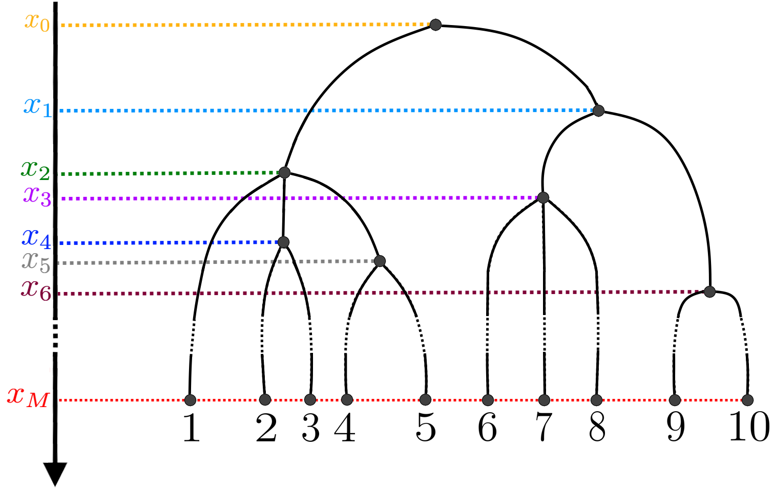
Figure 7: A tree with ten leaves. The overlap of leave (1) with the leaves ($2\cdots 5$) is $q(x_{2})$ and with the leaves ($6\cdots 10$) is $q(x_{0})$; the overlaps of leave (2) with the other leaves are the same as leave (1), with the only difference that the overlap with the leave (3) is now $q(x_{4})$.

These can be generated through a coalescent process known as Bolthausen-Sznitman coalescent Bolthausen and Sznitman (1998), starting from $M$ leaves, and progressively reducing the number of branches through a Markov process of random collisions in a ”time” $t$. A direct branching algorithm can also be used Parisi et al. (2015), however, here we find it more convenient to use the coalescent .

The branching points of the tree are labeled by the time variable $t$ ($t\geq 0$). In the following, we call nodes both the branching points and the leaves (terminal nodes). The coalescence process is ruled by the function $P(k|b)=\frac{b}{(b-1)(k-1)k}$ which tells the probability of coalescence of $k$ nodes if at that time there are $b$ nodes. We start with $M$ nodes at time zero: in this case $b=M$. We chose a number $k\in\{2,...,b\}$ at random with probability $P(k|b)$ and we coalesce $k$ nodes at random into a single one. In this way $b$ decrease to $b-k+1$. At the same moment, the time variable is incremented by a random $\Delta t$ with an exponential distribution and with average $\overline{\Delta t}=1/(b-1)$. The process stops at a finite time when $b=1$ and no more coalescence is possible.

At each level, $t$ is associated with a value $x(t)=x_{M}\exp(-t)$: the overlap between the branches that meet at that level is given by $q=q(x(t))$.

This is the only point where the function $P(q)$ appears in the construction. In our case, we obtain this $P(q)$ from the numerical data (see below for further details). Once the tree is built, one needs to associate random weights to the leaves. If $M$ is large, this is simply done by generating $M$ i.i.d. variables $u_{\alpha}$, for $\alpha=1,...,M$ with distribution $p(u)=x_{M}\theta(u-1)u^{-1-x_{M}}$, and defining the weights $w_{\alpha}=u_{\alpha}/\sum_{\gamma}u_{\gamma}$. Notice that in this construction both the weights and the overlaps associated with the given branching levels are independent of the tree’s structure. The values of $x_{M}$ and of $x(q)$ depend on the specific system at hand and should be given as input at the beginning of the computation.

The magnetizations $m_{\alpha}$ are zero mean Gaussian random variables with covariance $\overline{m_{\alpha}m_{\beta}}=q_{\alpha\beta}$ and they can be constructed efficiently in many ways. More details are provided in the SI.

Comparison with numerical simulations

We simulate Ising spin glass models at equilibrium in their low-temperature phase.

The Hamiltonian of a system with $N$ spins in a field reads

$${\cal H}=-\sum_{(i,j)\in{\cal E}}J_{ij}S_{i}S_{j}-\frac{h}{\sqrt{N}}\sum_{i=1}^{N}S_{i}$$ (6)

Where $\cal E$ denotes the set of edges of the graph where the model is defined: in our case either a Bethe lattice spin glass on a Random Regular Graph with coordination number equal to 4, or the 4D Edwards-Anderson model with periodic boundary conditions in a hypercubic lattice.

In a finite volume, the function $P(q)$ is measured as the probability distribution of the overlap between two equilibrium configurations (the replicas denoted as $\sigma$ and $\tau$) $q=\sum_{i}\sigma_{i}\tau_{i}/N$. We measure the probability $P(q)$ at $h=0$ and the probabilities $P_{C}(|q|;h)$ and $P(q;h)$ as a function of $h$ at low temperatures. In both cases, optimized code based on parallel tempering and multispin coding with 128 bits has been used. In Fig. 1 we show the results for the probability $P(|q|)$ for both systems at zero magnetic field.

From our numerical data, we extrapolate the functions $x(q)$ from these probability distributions at infinite volume. For each simulated volume, we approximate $P(q)$ with $P_{\mathrm{fit}}(q)=a+bq^{2}+(1-x_{M})\delta(q-q_{\mathrm{EA}})$: so, $x(q)=aq+bq^{3}/3$ and $x_{M}=x(q_{\mathrm{EA}})$. Then we fit the values of $a$ and $b$ using the data in the low $q^{2}$ region and we fix $q_{\mathrm{EA}}$ such that the mean value $\overline{\langle|q|\rangle}$ computed with $P_{\mathrm{fit}}(q)$ coincides with that obtained in the numerical simulation for that particular volume. In this way, we find that the position of the peak at that given volume is only a few percent off the estimated $q_{\mathrm{EA}}$ (see the SI). Using this representation $P_{\mathrm{fit}}(q)$ of the function $P(q)$ we have all the information to assign the weights of the leaves in the building process of the tree (see above). The predictions from the random trees have been averaged over $10^{5}$ trees with $10^{5}$ leaves: all the results are stable toward a variation of the number of leaves and the statistical errors are small.

We concentrated our attention on $\overline{\langle|q|\rangle}$ because we know that for large values of $h$ the magnetic susceptibility depends linearly on it (see the SI).

The reader may note that the theoretical curves of the probability distributions appearing in Fig. 2 and Fig. 3 are labeled with the superindex $N$ which, in the theoretical case, it is not associated with any size of the system. This superindex refers to the numerical curve (associated to a finite lattice with $N$ spins) from which the $P_{\mathrm{fit}}(q)$ is obtained following the above-explained process. In particular, the value $x_{M}$ used as the input in the construction of the tree depends on $N$ and this dependence is inherited by the tree.

An alternative approach would be to extrapolate the function $P(q)$ to infinite volume and to use this extrapolated function for the analytic computation. We have not followed this approach because using no extrapolation is more robust and allow us to make predictions also having only one value of $N$.

SUPPORTING INFORMATION

SI: Some technical details on the analytic computation

In the RSB theory in the infinite volume limit, each sample, i.e. each choice of the couplings $J$, is characterized by the weight of the states, their mutual overlap, and their magnetizations. These quantities fluctuate from sample to sample, the theory therefore deals with the probability distribution of these quantities. Ultrametricity implies that for each sample the states can be considered as the leaves of a tree, where the leaves carry a weight. Our task here is to generate numerically the weighted trees with the correct probability distribution.

In the real world quantities like the $P_{J}(q)$ depend on the system via the couplings $Js$: in the analytic approach one determines the probability distribution of the probability distribution $P_{J}(q)$. The simplest way to determine the probability of probabilities is by describing an algorithm that generates it. To this end, we show how to compute a $P_{\mathrm{Tree}}(q)$ that depends on the tree in such a way that in the large volume limit, $P_{J}(q)$ and $P_{\mathrm{Tree}}(q)$ have the same statistical properties.

Through random trees, we can approximate the distribution of spin-glass Gibbs measure in the thermodynamic limit. For the purposes of this work, we need for a given sample:

• A set of $M$ weights $w_{\alpha}$ for each state $\alpha=1,...,M$.

• A matrix of the overlaps $q_{\alpha\gamma}$.

• A set of Gaussian magnetizations $m_{\alpha}$ with covariances $\overline{m_{\alpha}m_{\gamma}}=q_{\alpha\gamma}$.

The first difficulty is that in the theory the number of leaves of the states is infinity. However, if we replace infinity by a large number we only commit a small error. If we neglect the leaves that have a weight less than $\epsilon$, the pruned tree remains with a finite number $M$ of leaves ($M=O(\epsilon^{-x_{M}})$). Moreover, in the limit where the cutoff $\epsilon$ goes zero (or $M$ goes to infinity), the interesting quantities averaged over the weighted pruned trees reproduce the same quantities averaged over the infinite weighted trees.

In principle, it is easy to generate trees according to the algorithm described in the text. However, it is not immediate to write an efficient code. There are many possibilities. Let us describe our choices. The random weights are easily constructed:

$$u_{\alpha}=\exp(x_{M}\log(r_{\alpha})),\ \quad w_{\alpha}=\frac{u_{\alpha}}{\sum_{\gamma=1}^{M}u_{\gamma}}\,,$$ (7)

where $r_{\alpha}$ are i.i.d. random numbers that are uniformly distributed inside the interval $[0,1)$. Notice that the minimum weight $w_{\min}$ is of order $\epsilon_{M}\sim M^{-1/x_{M}}$. Depending on the value of $x_{M}$ and the perturbation, the value of $M$ may be adequate (or not).

We then build up the tree with the aid of two variable length lists:

• The list of the identifiers (IDs) of the active nodes contains the nodes that have not yet coalesced and do not yet have a parent.

• The list of all nodes present at a given moment. Each node, indexed by its ID, is represented by a structure that contains the time at which it has been created and a variable $v$ conventionally equal to $-1$ if the node is active and equal to the ID of the parent node if the node has coalesced.

In addition, we have the time variable $t$. Let’s call $M(t)$ and $b(t)$ respectively the total number of nodes and the number of active nodes at time $t$. Clearly, $M(0)=b(0)=M$, while for large $b(t)$ we have approximately $b(t)\simeq M^{e^{-t}}$.

We repeat the following procedure up to the moment $t_{\mathrm{fin}}$, when $b(t_{\mathrm{fin}})=1$, i.e. there is only one surviving node, so no further coalescence is possible.

• We increment the time variable $t$ by a random $\Delta t$ with an exponential distribution and average $1/(b(t)-1)$: $\Delta t=-\log(r)/(b(t)-1)$ where $r$ is a random number uniformly distributed inside the interval $[0,1)$.

• We chose a number $k\in\{2,...,b(t)\}$ at random with probability $P(k|b(t))=\frac{b(t)}{(b(t)-1)(k-1)k}$ and we coalesce $k$ nodes chosen at random into a single one. In this way $b$ decreases to $b-k+1$ (i.e. $b(t+\Delta t)=b(t)-k+1$).

• We thus add a new node to both lists of nodes: its timestamp is set equal to $t+\Delta t$, its variable $v$ is set to -1 and its ID is equal to the last ID created incremented by one.

• We add to the $k$ branching nodes the information on the parent, and we remove them from the list of active nodes.

• We stop when only a single node is active.

When we stop only the root of the tree has an ID of the parent equal to $-1$. In this construction, the time stamp of the node increases with the ID number. We would like to stress that up to this point the construction of the tree is universal, i.e. it is the same for any value of $x_{M}$ (if we neglect the weights) and any function $q(x)$. The construction of the magnetizations can be done as follows, scanning the tree from the root to the leaves

• To each node, we assign an overlap given by $q(x_{M}\exp(-t))$.

• We start with the root and we assign to it a root magnetization that is equal to $r_{g}\sqrt{q_{\text{root}}}$, where $r_{g}$ is a Gaussian random number with variance one.

• We now scan the list of the nodes and we set

  $$m_{\text{node}}=m_{\text{parent}}+r_{g}\sqrt{q_{\text{node}}-q_{\text{parent}}}\,.$$ (8)

• In this way, the magnetization of the leaves are Gaussian random variables with the required covariance, $\overline{m_{\alpha}m_{\gamma}}=q_{\alpha\gamma}$, as it can be readily checked.

It is in principle straightforward to compute quantities like:

$$P_{J,C}(q;h)=\sum_{\alpha,\gamma}w_{\alpha}w_{\gamma}(h)\delta(q-q_{\alpha\gamma})\,.$$ (9)

However, the sum contains $M^{2}$ terms, which is computationally heavy for large $M$.

A fast approximate computation consists of the following. Let $\epsilon_{M}$ be the minimum value of $w_{\alpha}$ ($\epsilon_{M}=O(M^{-1/x}))$. We can neglect pairs with $w_{\alpha}w_{\gamma}(h)<\epsilon_{M}$. The number of the surviving terms is of order $O(M\log M)$ and we can restrict the sum to these terms if we order both the $w_{\alpha}$ and the $w_{\gamma}(h)$ in decreasing order and sum over $\alpha$ and $\gamma$ using two nested loops.

A final warning: most of the computer time may be spent in the computation of the $O(M^{2})$ overlaps. There are many possible ways to do this computation and one should be careful in using an efficient one that exploits the tree structure of the states.

In the end, the computational time can be reduced from a naive $O(M^{2})$ to $O(M(\log M)^{z})$. The exponent $z$ is likely equal to 2, but we have not measured the precise timings.

Average Magnetization

Let us study the average magnetization $m(h)$ in the presence of the field $h$. As in the main text, we define $m$ as the total magnetization divided by $N^{1/2}$ in such a way that for large $h$ the quantity $m(h)/h$ becomes the susceptibility. In principle, two phenomena contribute to the average magnetization:

• Within each state, the usual fluctuation-dissipation theorem holds, and the magnetic field increases the average magnetization by an amount of $\beta h(1-\overline{m_{\alpha}^{2}})=\beta h(1-q_{\mathrm{EA}})$

• As we have at length discussed, states with higher average magnetization $m_{\alpha}$ become more likely in the presence of the field $w_{\alpha}\to w_{\alpha}(h)$.

Taking care of both contributions we find

$${m(h)}=\beta h(1-q_{\mathrm{EA}})+\overline{\sum_{\alpha}w_{\alpha}(h)\tanh(\beta hm_{\alpha})m_{\alpha}}\,.$$ (10)

The second term in the previous equation can be readily computed using the same strategy as before by averaging over randomly generated trees. Moreover, integration by parts over the Gaussian distribution of the $m_{\alpha}$ reveals that the last term equals to

$$\begin{split}&\overline{\sum_{\alpha}w_{\alpha}(h)\tanh(\beta hm_{\alpha})m_{\alpha}}=\\ &\beta h\bigg{(}q_{\mathrm{EA}}-\overline{\sum_{\alpha\beta}w_{\alpha}(h)w_{\beta}(h)\tanh(\beta hm_{\alpha})\tanh(\beta hm_{\beta})q_{\alpha\beta}}\bigg{)}=\\ &\beta h\big{(}q_{\mathrm{EA}}-\langle q\rangle_{h}\big{)}\,.\end{split}$$ (11)

Putting the two terms together, we finally find

$$m(h)=\beta h\left(1-\int_{-1}^{1}\mathrm{d}q\,qP(q;h)\right)=\beta h\big{(}1-\langle q\rangle_{h}\big{)}\,.$$ (12)

The quantity $m(h)/h$ is equal to $\beta$ at $h=0$ and goes to the thermodynamic susceptibility $\chi=\beta\int_{0}^{1}\mathrm{d}x\;q(x)$ for large $h$.

SI: Simulation details

4D Edwards-Anderson

We have studied the 4D EA model in the presence of an external magnetic field. Its Hamiltonian is given by  (6) where $N=L^{4}$ is the total number of spins living in a hypercubic lattice of size $L$ with periodic boundary conditions. The couplings $J_{ij}$ are drawn from a bimodal probability distribution: it can be $\pm 1$ with a 50 % probability.

The disorder realization is quenched, i.e. the couplings remain constant through the whole simulation, defining what it is usually called a sample. Moreover, we have simulated different replicas, which are different simulations of the same sample evolving with different thermal noise.

Due to the toughness of the thermalization process in the simulation of spin glasses, it is convenient to speed up the convergence to the equilibrium by using different techniques. In our particular case, we have used a Multispin Coding Monte Carlo simulation Friedberg and Cameron (1970); Jacobs and Rebbi (1981) and we have taken advantage of the long binary registers that current CPUs can operate with: they allow us to simulate 128 samples at once. A set of 128 samples that are simulated together by using Multispin Coding is called a super-sample. We have also performed a parallel tempering Hukushima and Nemoto (1996); Marinari (1998) proposal every 20 Monte Carlo Sweeps. A detailed explanation of the implementation for the six-dimensional case in a magnetic field can be found in Ref. Aguilar-Janita et al. (2023).

We have simulated lattice sizes running from $L=5$ to $L=9$ with all the values of the external magnetic field in the set $h=\{0,1,2,4,6,8,10\}$. For each lattice size, we have simulated 20 $\times$ 128 samples. The same set of 20 $\times$ 128 samples has been simulated for the seven different values of the external magnetic field given above. Moreover, for each sample, we have simulated two replicas. The number of temperatures of the parallel tempering depends on the system size, but our work focuses on $T=0.7T_{\mathrm{c}}\approx 1.421$ so this temperature is always the lowest one.

$L$	#Samples	#Temp.	$T_{\mathrm{min}}$	$T_{\mathrm{max}}$
5	20 $\times$ 128	12	1.421	2.800
6	20 $\times$ 128	18	1.421	2.800
7	20 $\times$ 128	24	1.421	2.800
8	20 $\times$ 128	32	1.421	2.800
9	20 $\times$ 128	36	1.421	2.800

Table 1: Some parameters of our simulation. The first column refers to the linear size of the hypercube. The number of spins is $N=L^{4}$. In the second column, we present the number of samples analyzed, the specification $\times 128$ refers to the fact that each of the 20 super-samples contains 128 independent samples. The third column shows the number of temperatures simulated for each size. This number has been chosen in a way that ensures the random walk-in temperatures is sufficiently ergodic. Finally, the fourth and fifth columns refer to the lower and upper values of the temperature interval.

To ensure that we are working at equilibrium, the thermalization process must be monitored sample by sample. In this work, we use the thermalization protocol originally appearing on Ref. Billoire et al. (2018) which we briefly explain here for convenience.

We first determine with preliminary runs a sufficiently large number of Monte Carlo steps for most of the samples to be thermalized, and then we simulate our 20 super-samples that number of Monte Carlo steps. Along the simulation, we record the random walk in the temperatures of the parallel tempering and we use this information to compute the integrated autocorrelation time $\tau_{\mathrm{int},f}$ for several observables $f$, related to the random walks Billoire et al. (2018). We use now the largest value of those integrated autocorrelation times, $\tau_{\mathrm{int},f*}$, to estimate the exponential autocorrelation time by assuming that $\tau_{\mathrm{int},f*}\sim\tau_{\mathrm{exp}}$. Finally, we impose the criteria that a sample is considered thermalized when it has been running for a number of Monte Carlo steps thirty times bigger than $\tau_{\mathrm{exp}}$.

It is possible that, inside a super-sample, all the samples are thermalized except a few ones. In that case, we take the last configuration of the non-equilibrated samples and extend the simulation as long as necessary to reach the above-exposed thermalization criteria.

Spin glasses on Bethe lattices

To study spin glasses in a field on Bethe lattices we have considered the Hamiltonian in (6) where $\mathcal{E}$ is the edge set of a random regular graph of fixed degree 4. The couplings $J_{ij}$ are drawn from a bimodal probability distribution: $J_{ij}=\pm 1$ with a 50 % probability. For each sample, we have simulated 4 replicas without a field ($h=0$) and 4 replicas in a field, with several field intensities ($h\in\{1,2,4,8,16\}$).

We have sped up the simulation with the same techniques used in the 4D case, namely multi-spin coding and parallel tempering. In the multi-spin coding, we have used words of 128 bits, which allows us to simulate in parallel 128 systems sharing the same interaction graph topology while having different random couplings. We then average over a large number of different random regular graphs of fixed degree 4: this number is the first one in the column “#Samples” in Table 2 and is reported with a range [min-max] since a different computational effort has been devoted to different values of $h$ (the largest number of samples is the one always corresponding to the values of $h$ reported in the Figures in the main text).

In the parallel tempering algorithm, we have performed an attempt to swap temperatures every 32 Monte Carlo sweeps. The temperature schedule has been optimized following the “0.23 rule” Pelissetto and Ricci-Tersenghi (2014) and imposing $T_{\text{min}}=0.5T_{c}$ and $T_{\text{max}}=1.5T_{c}$, where $T_{c}=1/\text{arctanh}(1/\sqrt{3})\simeq 1.518651$ is the spin glass critical temperature. For the three sizes that we have simulated the number of temperatures used is reported in Table 2 in the column “#Temp”.

The column “#MCS” in Table 2 corresponds to the number of Monte Carlo sweeps we have run in each simulation. Typically the thermalization time (thanks to the use of the parallel tempering algorithm) is much smaller than that number. We have checked that the results obtained in the last half of the simulation are statistically equivalent to those obtained in the preceding quarter of the simulation. Data presented in the paper always corresponds to measurements obtained in the last half of the simulation. Moreover, the errors (when reported) have been always obtained only from graph-to-graph fluctuations: in this way, errors are somehow overestimated but are certainly insensitive to any correlation between measurements taken on the same sample and even on the same graph (with different couplings).

$N$	#Samples	#Temp.	#MCS
256	$[75005-144114]\times 128$	8	65536
1024	$[7614-11463]\times 128$	15	65536
4096	$1120\times 128$	28	262144

Table 2: Parameters of the simulations performed on Bethe lattices with fixed degree 4. A description of the parameters is provided in the text.

SI: Analysis details

Computation of the $P(q)$

The basic quantity we are interested in is the overlap $q$. To compute this observable we need to know the spin field of two different replicas $\sigma$ and $\tau$ at equilibrium

$$q=\dfrac{1}{N}\sum_{i}\sigma_{i}\tau_{i}\,,$$ (13)

where the sum runs over all the spins of the system and $N$ is the total number of spins.

Computationally, we take advantage of the Multispin Coding technique used to simulate our system. Since our CPU can perform binary operations over 128-bit words and we have recorded configurations from 128 samples at the same place, we use this previous setup to compute packages of 128 overlaps at once.

The main observable of our work is the overlap probability distribution $P(q)$. First, we compute a $P_{J}(q,L)$ for each one of the $2560$ samples and for each value of the field $h$. To do it we just take $10^{4}$ measures of the overlap $q$, as explained above, and build a histogram of frequencies. To avoid asymmetries induced by the binning process, we use one bin for each one of the $L^{4}+1$ possible different values of the overlap. Finally, we conveniently normalize the histogram to obtain a $P(q)$ such that $\int_{-1}^{1}\mathrm{d}q\leavevmode\nobreak\ P(q)=1$. Once we have a $P_{J}(q)$ for each sample, we perform the average over the disorder and compute the error bars for each bin using the Jackknife method  Young (2015); Efron (1982).

Once we have computed the $P(q,L)$, we want to obtain the position of the peaks, $q_{\mathrm{max}}(L)$, for the $h=0$ case. For this case, RSB predicts that the two symmetric peaks observed at $L$ become two Dirac deltas at $q_{EA}$ in the thermodynamic limit. In this section, we consider only positive values of $q$ and the symmetrized version of $P(q)$.

To obtain $q_{\mathrm{max}}(L)$ we begin by smoothing the $P(q)$ by taking its convolution with a Gaussian of width $1/\sqrt{8N}$. We define this smoothed version $\mathcal{P}(q)$ as

$$\mathcal{P}(q=c)=\int_{-\infty}^{\infty}\mathrm{d}q^{\prime}P\left(q^{\prime}\right)\mathcal{G}_{8N}\left(c-q^{\prime}\right),$$ (14)

where

$$\mathcal{G}_{8N}(x)=\sqrt{\frac{8N}{2\pi}}\mathrm{e}^{-8Nx^{2}/2}.$$ (15)

Now, working with the new $\mathcal{P}(q)$, we fit the neighborhood of the peak to a third-order polynomial and define $q_{\text{max}}(L)$ as the maximum of this polynomial. We say that a given point belongs to the neighborhood of the peak if its height surpasses a value of $0.9$ times the maximum height of the $\mathcal{P}(q)$. The values of $q_{max}(L)$ obtained by this procedure can be checked in Table  3. As explained in the Materials and methods section of the main article, the position of the peak at a given volume is only a few percent of the estimated $q_{\mathrm{EA}}(L)$. In Table 3 we also include the values of $q_{\mathrm{EA}}(L)$ used for the computation of the ultrametric trees.

$L$	$q_{\mathrm{max}}(L)$	$q_{\mathrm{EA}}(L)$
5	0.592(2)	0.625
6	0.574(2)	0.585
7	0.555(1)	0.568
8	0.543(1)	0.542
9	0.535(1)	0.530

Table 3: Position of the peaks $q_{\mathrm{max}}(L)$ of the $P(q,L)$ and values of $q_{\mathrm{EA}}(L)$ for different values of the lattice size $L$ in the 4D EA model for $T=0.7T_{\mathrm{c}}\approx 1.421$.

Compuation of the $R$-ratios

Finally, we will discuss how we have computed numerically the $R$-ratios.

In Fig. 12, we compare the theoretical results for $R_{c}^{N}(|q_{\mathrm{EA}}|)$ and $R^{N}(-|q_{\mathrm{EA}}|)$ with the data for those observables obtained from the numerical simulations on the 4D EA lattice. However, in finite systems, the function $P(q)$ does not end abruptly at $q=q_{\mathrm{EA}}$ but has a tail of non-zero probability up to $q=1$. Therefore, the definition of this observable in finite lattice systems is not obvious. In Fig. 12, we compute $R_{c}^{N}(|q_{\mathrm{EA}}|)$ as the integral from $q=q_{\mathrm{EA}}$ to $q=1$, and analogously, we compute $R^{N}(-q_{\mathrm{EA}})$ as the integral between $q=-1$ and $q=-q_{\mathrm{EA}}$. In particular:

$$R_{C}^{N}(|q_{\mathrm{EA}}|;h)=\frac{\int_{q_{\mathrm{EA}}}^{1}\mathrm{d}q\leavevmode\nobreak\ P_{C}^{N}(q;h)}{\int_{q_{\mathrm{EA}}}^{1}\mathrm{d}q\leavevmode\nobreak\ P^{N}(q;0)}\;,$$ (16)

and

$$R^{N}(-q_{\mathrm{EA}};h)=\frac{\int_{-1}^{-q_{\mathrm{EA}}}\mathrm{d}q\leavevmode\nobreak\ P_{C}^{N}(q;h)}{\int_{-1}^{-q_{\mathrm{EA}}}\mathrm{d}q\leavevmode\nobreak\ P^{N}(q;0)}\;.$$ (17)

Similar results can be obtained if one defines $R_{c}^{N}(|q_{\mathrm{EA}}|)$ as an integral around the peak:

$$R_{C}^{N}(|q_{\mathrm{EA}}|;h)=\frac{\int_{q_{\mathrm{EA}}-\Delta}^{q_{\mathrm{EA}}+\Delta}\mathrm{d}q\leavevmode\nobreak\ P_{C}^{N}(q;h)}{\int_{q_{\mathrm{EA}}-\Delta}^{q_{\mathrm{EA}}+\Delta}\mathrm{d}q\leavevmode\nobreak\ P^{N}(q;0)}\;,$$ (18)

where we define the interval of integration $2\Delta$ as the maximum distance between the points that fulfill the condition of having a height greater than 0.8 times the height of the point at $q_{\mathrm{EA}}$. In fact, we use this definition of the observable to compute the results shown in Fig. 13.

In Figs. 4 and 5 we probe the functions $R_{C}$ and $R$ in the region $|q|<q_{\mathrm{EA}}$, for which we see that the dependence on the volume is rather mild. In the same pictures, we plot the theoretical predictions that have been computed averaging over $10^{5}$ trees with $M=10^{5}$ leaves. Remarkably, we see that the finite size effects in both the Bethe Lattice and the 4D system are qualitatively similar and that the data approach the theoretical curves as the volume becomes large.

We recall that we have plotted the extrapolated predictions also in the region beyond the peaks. A typical fit and the extrapolation is shown in Fig. 8. This procedure is somewhat arbitrary, but it affects only the behavior in the tails at $|q|>q_{\mathrm{EA}}$, i.e. a region that shrinks to zero in the infinite volume limit.

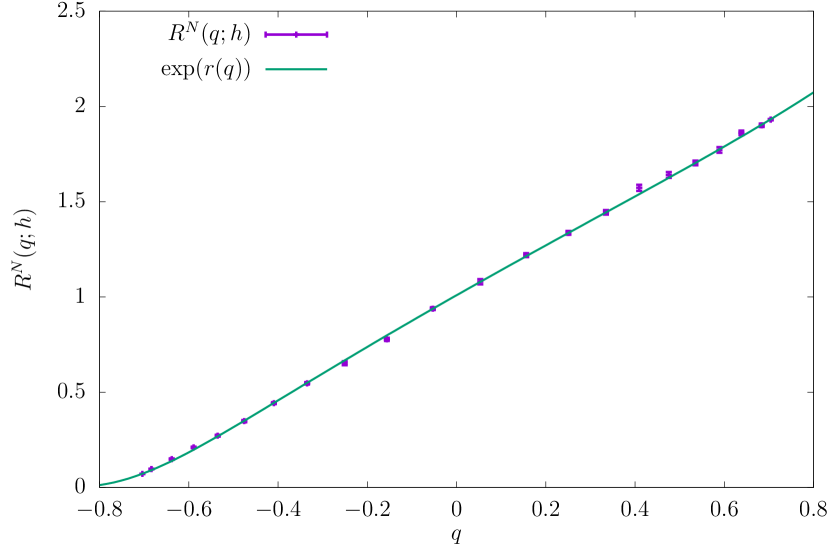
Figure 8: Analytic predictions for the function $R^{N}(Q)$ were obtained using the function $P(q)$ for the Bethe lattice, with the same parameters as in Fig. 2. We show the interpolating function or $|q|<q_{\mathrm{EA}}\approx 0.72$, (including the statistical error) and the extrapolations in the region $q_{\mathrm{EA}}<|q|<0.8$.

SI:A detailed comparison of analytic predictions and the numerical data

The functions $P$’s and $R$’s

In Figs. 9 and 10 we show the functions $P_{C}^{N}(|q|;h)$ and $P^{N}(q;h)$, respectively.

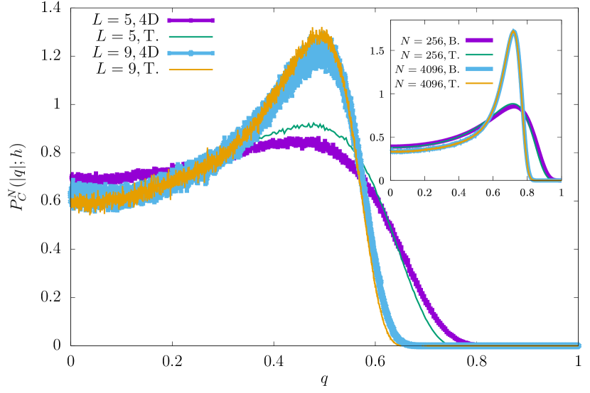
Figure 9: The function $P_{C}^{N}(|q|;h)$ versus $q$ at $T=0.7\;T_{c}$ for $h=10$ and different values of $L$ in the 4D EA model. Lines correspond to the theoretical prediction from the ultrametric tree (T.) and points with error bars correspond to simulations. Inset: The function $P_{C}^{N}(|q|;h)$ against $q^{2}$ at $T=057\;T_{c}$ for $h=4$ and different values of $N$ in the Bethe lattice.

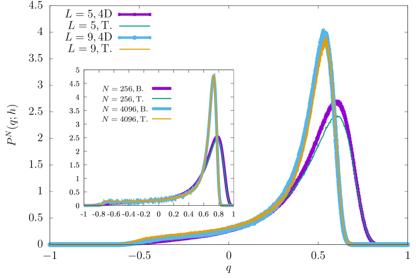
Figure 10: The function $P^{N}(q;h)$ versus $q$ at $T=0.7\;T_{c}$ for different values of $L$ in 4D EA model ($h=10$). Inset: $P^{N}(q;h)$ as a function of $q$ at $T=0.7\;T_{c}$ for different values of $N$ in Bethe lattice ($h=4$).

We see that for both functions, for small size, the analytic computations are less accurate but qualitatively correct: this should be expected as far as the analytic computations are exact only in the infinite volume limit. Moreover, the peaks are wider, and the tail of the peaks is quite large: in this situation, our fitting procedure for the function $P(q)$ has a higher degree of approximation. The important message is that the difference between theory and numerical data strongly decreases by increasing the volume.

In order to check if the general prediction that the function $P^{N}(|q|;h)$ does not depend on $h$, in Fig.11 we have plotted the ratio:

$$R_{A}^{N}(|q|;h)=\frac{P^{N}(|q|;h)}{P^{N}(|q|;0)}\,.$$ (19)

This ratio should be one in the infinite volume limit: we see that for smaller volumes the ratio is near but not exactly one, but approaches one for larger volumes. A peculiar property of RSB is that $R_{A}^{N}(|q|;h)$ is independent of $h$ while $R_{C}^{N}(|q|;h)$ is strongly dependent on $h$.

The reader may notice that we have plotted transparent bands instead of points in Fig. 11. We have, for each of the possible values of $|q|$, a value of the observable $R_{A}^{N}(|q|;h)$. The problem with plotting the points is that the value of $R_{A}^{N}(|q|;h)$ is too noisy and curves for different $L$’s (or different $N$’s for the Bethe case) overlap each other, hindering the visibility.

To solve this situation, we have defined a window around each value of $|q|$ and we have computed the mean $\mu_{q}$ and the standard deviation $\sigma_{q}$ for the points inside that window. Then, we have plotted the transparent bands of Fig. 11 with limits $\left[\mu_{q}-2\sigma_{q},\mu_{q}+2\sigma_{q}\right]$.

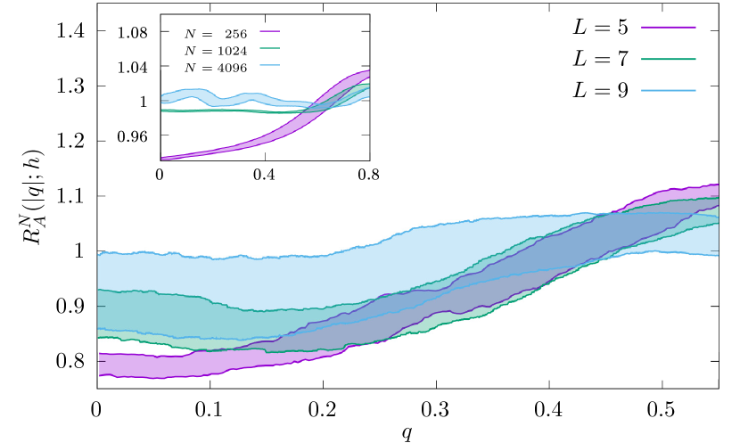
Figure 11: The ratio $R_{A}^{N}(|q|;h)$ as a function of $q$ at $T=0.7\;T_{c}$ for different values of $L$ in 4D EA lattice ($h=10$). Inset: ratio $R_{A}^{N}(q;h)$ as a function of $q$ at $T=0.5\;T_{c}$ for different values of $N$ in Bethe lattice ($h=4$).

In Figs. 9 and 10 we show the results for a given value of $h$. To study the dependence on the value of the magnetic field we focus on the values at $|q|=q_{\mathrm{EA}}$: we depict in Fig. 12 the ratios $R^{N}(-q_{\mathrm{EA}};h)$ and $R_{C}^{N}(|q_{\mathrm{EA}}|;h)$ as a function of $h$. Theory and simulations qualitatively agree also for small systems, and their difference decreases when increasing the volume. Both quantities should go to zero asymptotically at large $h$. A detailed analysis Franz et al. (2024) tells us that the chaos ratio $R_{C}^{N}(|q_{\mathrm{EA}}|;h)$ goes to zero as $\exp(-Ah^{2})$. Unfortunately, numerically it is hard to see that behavior. We need to sample the region $h\gg 1$: for not too large $N$ this requirement conflicts with the need to stay at a small total magnetic field $H=hN^{-1/2}$ as required by our simulations (see the large finite-size effects that are present already at the not-very-large fields we have used). Also, the analytic techniques we use (random generators of the trees) are not well suited for large $N$ because it would require the generation of an exponentially large number of leaves.

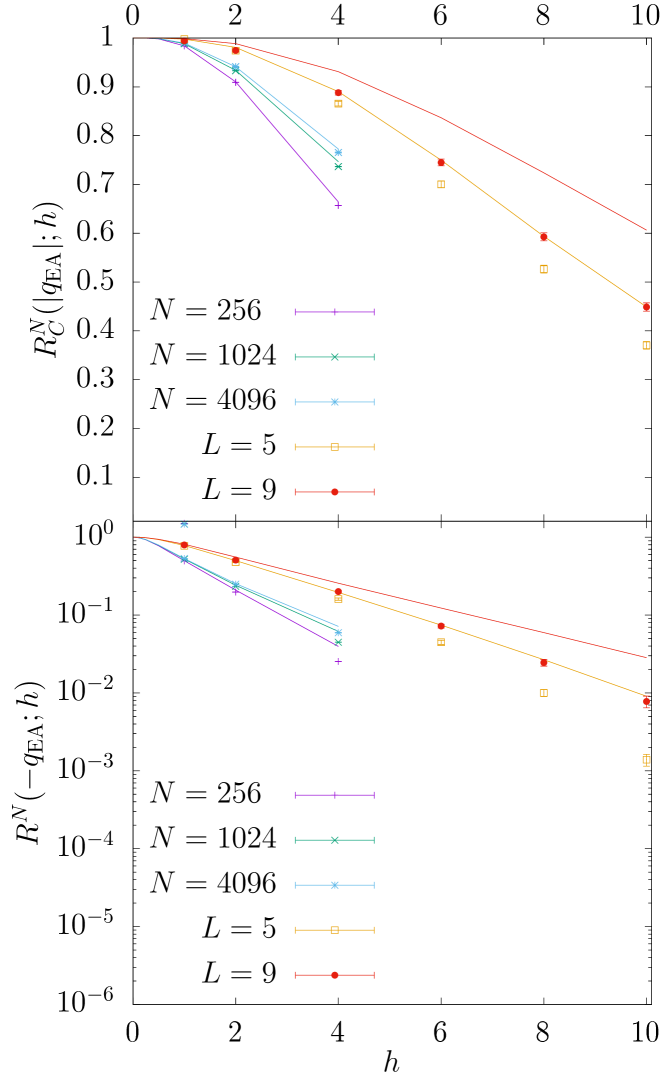
Figure 12: Top: The ratio $R_{C}^{N}(|q_{\mathrm{EA}}|;h)$ at $T=0.7T_{c}$ for different values of $N$ in the Bethe lattice and of $L$ in 4D EA. Lines correspond to the theoretical prediction. Bottom: The ratio $R^{N}(-q_{\mathrm{EA}};h)$ at $T=0.7T_{c}$ for different values of $N$ in the Bethe lattice and of $L$ in the 4D EA. Lines correspond to the theoretical prediction.

Large deviations in the negative tails

To study the large deviations in the negative tails of $P^{N}(q,h)$ we design the following procedure. Firstly, let us define

$$I_{J}(h)=\int_{-q_{\mathrm{EA}}-\Delta}^{-q_{\mathrm{EA}}+\Delta}\mathrm{d}q\leavevmode\nobreak\ P_{J}^{N}(q,h)\,.$$ (20)

Notice that we have an integral $I_{J}(h)$ for each $J$-sample and magnetic field. Next, for a given value of $h$, we sort these integrals from the lowest value to the highest one, denoting the newly ordered set of integrals (as a function of the sample number) as $I_{J^{o}}(h)$. Finally, we define

$$R_{<,{J^{o}}}^{N}(-q_{\mathrm{EA}};h)=\frac{I_{J^{o}}(h)}{I_{J^{o}}(0)}\,.$$ (21)

We remark that each $h$ has its own ordered set of couplings $J^{o}$, and that this order could change from different values of $h$, including $h=0$.

With these $R_{<,{J^{o}}}^{N}(-q_{\mathrm{EA}};h)$ values we compute the cumulative probability distribution $\mathrm{Prob}(R_{<,{J^{o}}}^{N}(-q_{\mathrm{EA}};h)<R)$.

We notice the agreement is excellent for not too small $R$ with the exclusion of the highest fields. However, for this observable for $h=10$ the numerical data show a very strong dependence on the size of the system.

If we look at small values of $R$ we find that the numerical cumulative is higher than the analytic predictions: in other words, the tail at smaller values of $R$ is higher than the theoretical predictions, i.e. we miss samples in the region of $0<R<.1$ and we have an excess of samples with $R=0$. These results should not be surprising: we have run the simulations up to 30 times the thermalization time in our thermalization criteria. Consequently, regions of phase space with a probability lower than 1/30 may be missed. It is quite possible that the discrepancy between theory and numerical simulations at not too large $h$ would strongly decrease with much longer simulations.

In Fig. 13 we confront the numerical data from the 4D EA model with the theoretical result for this cumulative probability. We show data for $h=2,4,6$, and 10 and for the largest simulated lattice $L=9$. We find good agreement for small and intermediate values of $h$ which deteriorates for very large values of $h$.

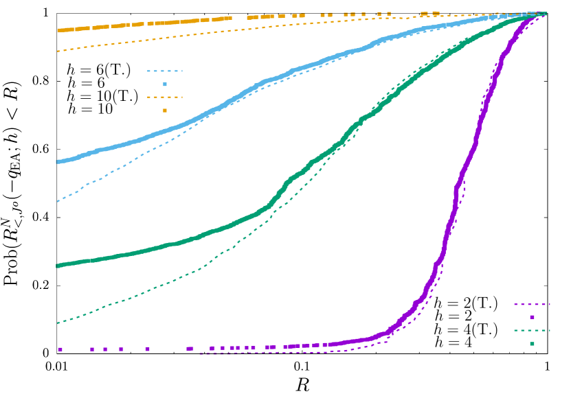
Figure 13: Theory and 4D EA data for $\mathrm{Prob}(R_{<,{J^{o}}}^{N}(-q_{\mathrm{EA}};h)<R)$ as a function of $R$, for $h=2,4,6$ and 10 and $L=9$. Dashed lines correspond with the theoretical prediction.