Universal and robust quantum coherent control based on a chirped-pulse driving protocol

Abstract

We propose a chirped-pulse driving protocol and reveal its exceptional property for quantum coherent control. The nonadiabatic passage generated by the driving protocol, which includes the population inversion and the nonadiabaticity-induced transition as its ingredients, is shown to be robust against pulse truncation. We further demonstrate that the protocol allows for universal manipulation on the qubit system through designing pulse sequences with either properly adjusted sweeping frequency or pulsing intensity.

I Introduction

Exquisite control over the dynamics of quantum systems is highly sought after in various fields of quantum physics and engineering, including atomic interferometry weitz1994 ; butts2013 ; kumar2013 , quantum-limited metrology giov2006 ; boixo2007 ; yang2022 , information processing for qubit systems nielsen , and so on. In particular, achieving quantum gate operations with sufficient accuracy that surpass the error thresholds of quantum error correcting codes knill2005 ; preskill2006 is a crucial aspect in realizing scalable quantum computation. A variety of fault-tolerant techniques, e.g., geometric quantum manipulation zanardi1999 ; jones2000 ; duan2001 ; toyoda2013 ; review2023 , dynamically corrected gates dcg1 ; dcg2 ; dcg3 as well as numerical optimization kha2005 ; song2022 , have been proposed to implement coherent manipulation for quantum states and information processing, aiming to address imperfections in fabrication or the decoherence induced by the environmental noise.

Utilization of chirped pulses in driven quantum systems is able to produce robust state transfer, which has been incorporated into quantum control schemes such as rapid adiabatic passage melinger1992 ; vitanov2001 ; netz2002 and the composite pulse sequences brown2004 ; toro2011 . Comparing with the conventional resonant $\pi$-pulse scheme pi2002 , the adiabatic passage of the chirped-pulse driving offers the advantage of being insensitive to the pulse area. On the other hand, the occurrence of avoided level crossings in such driven systems can exhibit diverse dynamical behavior related to the nonadiabatic evolution. For example, the adiabatic population transfer would be damaged by the nonadiabaticity-induced transition, e.g., in the well-known Landau-Zener model landau ; zener , whereas this state transferring will be retained under the nonadiabatic evolution in some of its variants yang2018 ; li2018 . Moreover, chirped pulses assume an ideal infinite field intensity, which often results in the generation of a divergent dynamical phase. In realistic systems, field pulses are inevitably truncated at the starting and ending points. While this truncation may not significantly impact the fidelity of the wave function, it does present challenges in accurately controlling the phase factor. This, in turn, will affect the coherent dynamics during subsequent information processing.

In this paper, we propose a distinctive chirped-pulse driving protocol and demonstrate that its coherent dynamics is immune to the aforementioned pulse truncation. The key to this property lies in the fact that the total phase integrated over the nonadiabatic evolution of the driven quantum system converges to a finite value, despite the infinite chirped field. Consequently, we are able to reveal that the nonadiabatic passage, including the population inversion and the nonadiabatic transition generated by the dynamical evolution, is insensitive to truncation of the chirped pulse. Furthermore, we illustrate that this driving protocol enables universal manipulation on the qubit system by designing a pulse sequence with appropriately tuned frequency or field strength of the chirped pulses.

The remaining sections of the paper are organized as follows. In Sec. II we propose a chirped-pulse driven model and present an analytic approach to resolving exactly its nonadiabatic evolution governed by the time-dependent Schrödinger equation. The time evolution operator of the ideal driving protocol is shown to incorporate two elements: the population inversion and the nonadiabaticity-induced transition. Its explicit form is then elucidated in relation to different settings of the field parameters. In Sec. III, we reveal the robustness of the resulting coherent operation of the protocol in the presence of truncation of the chirped pulse. Moving forward to Sec. IV, we demonstrate how universal qubit manipulation can be achieved through designing a pulse sequence with adjustable field parameters. Finally, Sec. V provides a summary of the paper.

II Driven quantum model of the protocol and its exact solution

The driven quantum model of the chirped-pulse protocol that we are going to consider is described by the following time-dependent Hamiltonian

$$H(t)=\bm{\Omega}(t)\cdot\bm{J}=\eta\left[J_{x}+\frac{\nu t}{\sqrt{1-(\nu t)^{2}}}J_{z}\right],$$ (1)

where $J_{i}$ $(i=x,y,z)$ are angular momentum operators satisfying $[J_{i},J_{j}]=i\epsilon_{ijk}J_{k}$, and the amplitude $\eta$ and the frequency $\nu$ are given constants. The ratio of the two components of the scanning field $\bm{\Omega}(t)$, i.e., $\Omega_{z}(t)/\Omega_{x}=\frac{\nu t}{\sqrt{1-(\nu t)^{2}}}$, varies from $-\infty$ to $+\infty$ during $t\in(-1/\nu,1/\nu)$ (assuming $\nu>0$ herein), hence the instantaneous energy levels of the system undergo an avoided crossing (see Fig. LABEL:f_Omega_E). The system specifies a distinct example from those known paradigms such as the Landau-Zener model landau ; zener and tangent-pulse driven model yang2018 .

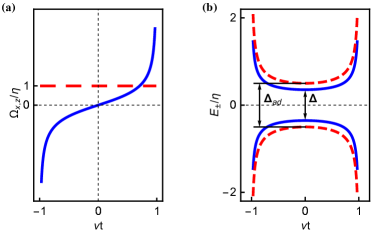
Figure 1: Chirped-pulse driving protocol specified by the Hamiltonian (1). (a) Field component $\Omega_{z}(t)$ (solid line) and $\Omega_{x}$ (dashed line) of the driving protocol; (b) The nonadiabatic energy described by $E_{\pm}(t)/\eta=\mp\frac{1}{2}\cos\varphi\csc\theta$ with $\nu/\eta=1$ (solid line) and adiabatic energy levels in the limit $\nu/\eta\rightarrow 0$ (dashed line). The corresponding gaps at the crossing point $t=0$ are shown to be $\Delta=1/\sqrt{2}$ and $\Delta_{ad}=1$, respectively.

figure]f_Omega_E

We now show that the wave function of the system governed by the Schrödinger equation (setting $\hbar=1$)

$$i\frac{\partial}{\partial t}|\psi(t)\rangle=H(t)|\psi(t)\rangle$$ (2)

can be solved analytically. To this end, we invoke a so-called gauge transformation wang1993 ; cen2003 ; ding2010 $G(t)=e^{i\theta(t)J_{y}}e^{i\varphi J_{x}}$, in which the angle $\varphi=\arccos\frac{\eta}{\sqrt{\eta^{2}+\nu^{2}}}$ and

$$\theta(t)=-\arccos\frac{\Omega_{z}(t)}{\Omega(t)}=-\arccos(\nu t).$$ (3)

The transformed state $|\psi^{g}(t)\rangle=G^{\dagger}(t)|\psi(t)\rangle$ is verified to satisfy a covariant Schrödinger equation $i\frac{\partial}{\partial t}|\psi^{g}(t)\rangle=H^{g}(t)|\psi^{g}(t)\rangle$ where the effective Hamiltonian reads

$$H^{g}(t)=G^{\dagger}H(t)G(t)-iG^{\dagger}\partial_{t}G(t)=\sqrt{\frac{\eta^{2}+\nu^{2}}{1-(\nu t)^{2}}}J_{z}.$$ (4)

That is to say, in the new representation with respect to the transformation $G(t)$, the system possesses a “stationary” solution $|\psi_{\pm}^{g}(t)\rangle=e^{\mp i\Theta(t,t_{0})}|\pm\rangle$, in which $|\pm\rangle$ denotes the eigenstates of $J_{z}$ with the magnetic quantum number $m=\pm\frac{1}{2}$ and the total phase $\Theta(t,t_{0})$ can be rigorously calculated as

$$\begin{split}\Theta(t,t_{0})&=\frac{1}{2}\int_{t_{0}}^{t}\sqrt{\frac{\eta^{2}+\nu^{2}}{1-(\nu t^{\prime})^{2}}}dt^{\prime}\\ &=\frac{1}{2}\sqrt{1+\frac{\eta^{2}}{\nu^{2}}}\bigg{[}\arcsin(vt)-\arcsin(vt_{0})\bigg{]}.\end{split}$$ (5)

Consequently, the basic solution to the original Schrödinger equation is obtained as

$$|\psi_{\pm}(t)\rangle=G(t)|\psi^{g}_{\pm}(t)\rangle=e^{\mp i\Theta(t,t_{0})}e^{i\theta(t)J_{y}}e^{i\varphi J_{x}}|\pm\rangle,$$ (6)

by which the nonadiabatic energy levels of the system, defined by $E_{\pm}(t)\equiv\left\langle\psi_{\pm}(t)|H(t)|\psi_{\pm}(t)\right\rangle$, is worked out to be $E_{\pm}(t)=\mp\frac{\eta}{2}\cos\varphi\csc\theta$. The avoided crossing phenomena of this nonadiabatic levels as well as the eigenvalues of $H(t)$ are depicted in Fig. LABEL:f_Omega_E(b).

Following the above result, the evolution operator of the system over any time interval $t\in(t_{0},t_{f})$ is obtained straightforwardly as

$$U(t_{f},t_{0})=G(t_{f})U^{g}(t_{f},t_{0})G^{\dagger}(t_{0}),$$ (7)

in which $U^{g}(t_{f},t_{0})=\exp[-i\Theta(t_{f},t_{0})J_{z}]$ denotes the one generated by $H^{g}(t)$ in the stationary representation. For the ideal overall evolution during $t\in(-1/\nu,1/\nu)$, one has $\theta(t_{0})=-\pi$ and $\theta(t_{f})=0$. Hence the evolution operator reads

$$U_{0}(\eta/\nu) \equiv U(-1/\nu,1/\nu)$$ (8)

$$= e^{i\varphi J_{x}}e^{-i2\Theta_{0}(\eta/\nu)J_{z}}e^{-i\varphi J_{x}}\times e^{i\pi J_{y}},$$

with $\Theta_{0}(\eta/\nu)=\sqrt{1+\frac{\eta^{2}}{\nu^{2}}}\frac{\pi}{2}$. The last factor $e^{i\pi J_{y}}\equiv i\sigma_{y}$ in the above expression of $U_{0}(\eta/\nu)$ indicates the population inversion induced by the chirped pulse. The product of the first three factors can be re-expressed as

$$\tilde{U}_{0}(\eta/\nu)=e^{-i2\Theta_{0}(\eta/\nu)J(\varphi)},J(\varphi)\equiv\sin\varphi J_{y}+\cos\varphi J_{z}.$$ (9)

It accounts for the nonadiabaticity-induced transition and is verified to recover a pure phase shift over the basis states $|\pm\rangle$ in the adiabatic limit $\nu/\eta\rightarrow 0$ (i.e., $\varphi\rightarrow 0$). Owing to the parameter-dependency of $\tilde{U}_{0}(\eta/\nu)$, late on we will demonstrate that universal manipulation on the qubit system can be implemented by a sequence of pulsed operations generated by the protocol with a tunable $\eta/\nu$.

The above obtained expression for the evolution operator is applicable to any real parameter $\eta$, but it is only valid for $\nu>0$. For a Hamiltonian formulated by Eq. (1) but with $\nu\rightarrow-\nu$, its relation to the original one can be described by a $\sigma_{x}$ flip: $H(t)\rightarrow\sigma_{x}H(t)\sigma_{x}$. So its generated evolution can be obtained by applying the same flip operation on $U_{0}(\eta/\nu)$:

$$U_{0}(\eta/\nu)\rightarrow\sigma_{x}U_{0}(\eta/\nu)\sigma_{x}=e^{i2\Theta_{0}(\eta/\nu)J(\varphi)}\times e^{-i\pi J_{y}}.$$ (10)

Moreover, if we perform further the transformation $\eta\rightarrow-\eta$ on the Hamiltonian with $-\nu$, the result of Eq. (10) is still valid just noticing that $\varphi\rightarrow\pi-\varphi$. At this stage, it is recognized that the resulting unitary evolution herein indicates an inverse operation of the original $U_{0}(\eta/\nu)$:

$$~{}~{}~{}e^{i2\Theta_{0}(\eta/\nu)J(\pi-\varphi)}\times e^{-i\pi J_{y}}$$

$$=e^{-i\pi J_{y}}\times e^{i2\Theta_{0}(\eta/\nu)J(\varphi)}\equiv U_{0}^{\dagger}(\eta/\nu),$$ (11)

where we have used the fact $J(\pi-\varphi)=e^{-i\pi J_{y}}J(\varphi)e^{i\pi J_{y}}$. This result can also be verified in view that the transformation of the parameters $(\eta,\nu)\rightarrow(-\eta,-\nu)$ indicates that $H(t)\rightarrow\sigma_{z}H(t)\sigma_{z}$, hence the evolution operator changes as $U_{0}(\eta/\nu)\rightarrow\sigma_{z}U_{0}(\eta/\nu)\sigma_{z}=U_{0}^{\dagger}(\eta/\nu)$.

III Robustness of the coherent operation against pulse truncation

One remarkable property of the above driven model, which distinguishes it from the Landau-Zener driving and other known analogs, is that despite the infinite intensity of the chirped pulse, it generates a finite total phase. In addition to the known advantage that population inversion is insensitive to the truncation at the ending points $t_{0,f}=\mp\tau$ as long as $\Omega_{z}(\tau)\gg\Omega_{x}$, this property also suggests that truncating the chirped pulses in the present model may have a lesser impact on the accumulated phase $\Theta_{0}(\eta/\nu)$ and, consequently, on the nonadiabaticity-induced transition specified by $\tilde{U}_{0}(\eta/\nu)$ in Eq. (9). That is to say, the coherent dynamics generated by this driving protocol would be robust against arbitrary truncation provided that $\Omega_{z}(\tau)/\Omega_{x}\gg 1$.

Figure 2: Fidelity of coherent operations yielded by the driving protocol with pulse truncation. (a) Fidelity $F(U_{0},U_{\delta})$ of the evolution operator with $\eta/\nu=1$ (blue solid line) and $\sqrt{3}$ (red dashed line); (b) Fidelity $F(\tilde{U}_{0},\tilde{U}_{\delta})$ of the corresponding elements responsible for the nonadiabaticity-induced transition in the dynamical evolution.

figure]fidelity

To be more specific, let us denote by $\delta\equiv\Omega_{x}/\Omega_{z}(\tau)$ the cutoff ratio of the field components of the chirped pulse. Following Eq. (5), the total phase integrated over $t\in(-\tau,\tau)$ is given by

$$\Theta_{\delta}(\eta/\nu)=\sqrt{1+(\eta/\nu)^{2}}{\rm arccot}\delta,$$ (12)

where we have used the relation $\nu\tau=(\delta^{2}+1)^{-1/2}$. The resulting time evolution operator, according to Eq. (7), is specified by

$$U_{\delta}(\eta/\nu)=e^{-i\arctan\delta J_{y}}\times\tilde{U}_{\delta}(\eta/\nu)\times e^{i(\pi-\arctan\delta)J_{y}},$$ (13)

in which $\tilde{U}_{\delta}(\eta/\nu)=e^{-i2\Theta_{\delta}(\eta/\nu)J_{\varphi}}$ with $J_{\varphi}$ shown in Eq. (9). The influence of the truncation on the coherent dynamical evolution can be conveniently characterized by the following fidelity:

$$F(U_{0},U_{\delta})=\frac{1}{4}{\rm Tr}[U_{0}^{\dagger}U_{\delta}+U_{\delta}^{\dagger}U_{0}].$$ (14)

Consider two particular settings of the dynamical parameter, say, $\eta/\nu=\sqrt{3}$ ($\varphi=\pi/6$) and $\eta/\nu=1$ ($\varphi=\pi/4$). For these two cases the total phases are worked out to be $\Theta_{0}(\eta/\nu)=\pi$ and $\pi/\sqrt{2}$, and the ideal chirped-pulse driving gives rise to a spin flip $U_{0}(\sqrt{3})=e^{i\pi J_{y}}$ (along the $y$ axis) and a composite flip operation $U_{0}(1)=e^{-i\pi(J_{y}+J_{z})}e^{i\pi J_{y}}$, respectively. For the practical driving process with pulse truncation, the corresponding evolution operator $U_{\delta}(\eta/\nu)$ is given by Eq. (13) with

$$\tilde{U}_{\delta}(\sqrt{3}) = e^{-i2{\rm arccot}\delta(J_{y}+\sqrt{3}J_{z})},$$

$$\tilde{U}_{\delta}(1) = e^{-i2{\rm arccot}\delta(J_{y}+J_{z})}.$$ (15)

We plot in Fig. LABEL:fidelity the fidelities $F(U_{0},U_{\delta})$ of the above two coherent operations with $\eta/\nu=\sqrt{3}$ and $1$ as well as $F(\tilde{U}_{0},\tilde{U}_{\delta})$ responsible for those of the nonadiabaticity-induced transition. For all these quantities, the numerical results display that the errors induced by the truncation could be reduced below the order of $10^{-3}$ as long as $\Omega_{z}(\tau)/\Omega_{x}\gtrsim 30$.

IV Universal qubit manipulation

Generally, an arbitrary single-qubit operation can be implemented by employing two non-commutative unitary transformations, e.g., the rotations along the $y$ axis $e^{i\phi_{y}J_{y}}$ and along the $z$ axis $e^{i\phi_{z}J_{z}}$. In the present protocol described by the Hamiltonian (1), while non-commutative $U_{0}(\eta/\nu)$’s can be achieved by setting different pulsing strength $\eta$ or sweeping frequency $\nu$, they distinctly differ from those conventional rotations along fixed axes. Therefore, it is interesting to inquire about the possibility and method of implementing universal manipulation on the qubit system by the present driving protocol. Below we provide an affirmative answer by outlining a pathway to this goal.

Let us start by rewriting the time evolution operator shown in Eq. (8) as

$$U_{0}(\eta/\nu)=r_{0}I_{2}+i\bm{r}\cdot\bm{\sigma},$$ (16)

where $r_{0}$ and $\bm{r}$ satisfy $r_{0}^{2}+\bm{r}^{2}=1$ and are specified by

$$r_{0}(\eta/\nu)=\sin\Theta_{0}\sin\varphi,$$

$$\bm{r}(\eta/\nu)=-\sin\Theta_{0}\cos\varphi\hat{e}_{x}+\cos\Theta_{0}\hat{e}_{y}.$$ (17)

We employ the evolution operators generated by a couple of consecutive driving pulses, i.e., $U_{0}(\eta/\nu)$ and $U_{0}(\eta^{\prime}/\nu^{\prime})=r_{0}^{\prime}I_{2}+i\bm{r}^{\prime}\cdot\bm{\sigma}$. Combining these two operations gives rise to

$$\mathcal{R}(\eta^{\prime}/\nu^{\prime},\eta/\nu)\equiv U_{0}(\eta^{\prime}/\nu^{\prime})U_{0}(\eta/\nu)=R_{0}I_{2}+i\bm{R}\cdot\bm{\sigma},$$ (18)

in which

$$R_{0}=r_{0}^{\prime}r_{0}-r_{x}^{\prime}r_{x}-r_{y}^{\prime}r_{y},~{}R_{x}=r_{0}r_{x}^{\prime}+r_{0}^{\prime}r_{x},$$

$$R_{y}=r_{0}r_{y}^{\prime}+r_{0}^{\prime}r_{y},~{}~{}~{}~{}~{}~{}~{}~{}~{}~{}R_{z}=r_{x}r_{y}^{\prime}-r_{x}^{\prime}r_{y}.$$ (19)

To proceed, we show the capability of the operation $\mathcal{R}(\eta^{\prime}/\nu^{\prime},\eta/\nu)$ to implement universal rotation on a spin initially along either the $y$ or the $z$ axis. Straightforwardly, we characterize the corresponding outcomes as $\mathcal{R}\sigma_{y}\mathcal{R}^{\dagger}=\bm{S}\cdot\bm{\sigma}$ and $\mathcal{R}\sigma_{z}\mathcal{R}^{\dagger}=\bm{T}\cdot\bm{\sigma}$, in which the two Bloch vectors $\bm{S}(\eta^{\prime}/\nu^{\prime},\eta/\nu)$ and $\bm{T}(\eta^{\prime}/\nu^{\prime},\eta/\nu)$ are specified by

$$S_{x}(\eta^{\prime}/\nu^{\prime},\eta/\nu)=2R_{0}R_{z}+2R_{x}R_{y},$$

$$S_{y}(\eta^{\prime}/\nu^{\prime},\eta/\nu)=R_{0}^{2}-R_{x}^{2}+R_{y}^{2}-R_{z}^{2},$$

$$S_{z}(\eta^{\prime}/\nu^{\prime},\eta/\nu)=-2R_{0}R_{x}+2R_{y}R_{z},$$ (20)

and

$$T_{x}(\eta^{\prime}/\nu^{\prime},\eta/\nu)=-2R_{0}R_{y}+2R_{x}R_{z},$$

$$T_{y}(\eta^{\prime}/\nu^{\prime},\eta/\nu)=2R_{0}R_{x}+2R_{y}R_{z},$$

$$T_{z}(\eta^{\prime}/\nu^{\prime},\eta/\nu)=R_{0}^{2}-R_{x}^{2}-R_{y}^{2}+R_{z}^{2},$$ (21)

respectively. The parametric surfaces of $\bm{S}(\eta^{\prime}/\nu^{\prime},\eta/\nu)$ and $\bm{T}(\eta^{\prime}/\nu^{\prime},\eta/\nu)$ are shown in Fig. LABEL:rotation. The universality of the rotation is justified by the fact that the function domains cover over the entire surface of the Bloch sphere through tuning appropriately the ranges of $\eta/\nu$ and $\eta^{\prime}/\nu^{\prime}$.

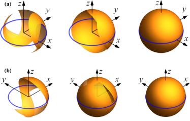
Figure 3: Schematic to illustrate the universality of the rotation $\mathcal{R}(\eta^{\prime}/\nu^{\prime},\eta/\nu)$ acting on $\sigma_{y}$ and $\sigma_{z}$. (a) Parameter surfaces of $\bm{S}(\eta^{\prime}/\nu^{\prime},\eta/\nu)$ in which the domains of $\eta/\nu$ and $\eta^{\prime}/\nu^{\prime}$ responsible for the left, middle, and right panels are $\eta/\nu\in(-1,1),(-2,2),(-3,3)$ and $\eta^{\prime}/\nu^{\prime}\in(-1,1),(-2,2),(-3,3)$, respectively. (b) Parameter surfaces of $\bm{T}(\eta^{\prime}/\nu^{\prime},\eta/\nu)$ with respect to the same domains of $\eta/\nu$ and $\eta^{\prime}/\nu^{\prime}$ specified in (a) for the left to right panels.

figure]rotation

With the above results, we are now able to show that the universal set of the gate operations $e^{i\phi_{y}J_{y}}$ and $e^{i\phi_{z}J_{z}}$ with $\phi_{y,z}\in(-\pi/2,\pi/2)$ can be achieved by applying the driving protocol. Specifically, one can exploit the following sequence of pulsed operations:

$$\mathcal{R}^{\dagger}(\eta^{\prime}/\nu^{\prime},\eta/\nu)U_{0}(\bar{\eta}/\bar{\nu})\mathcal{R}(\eta^{\prime}/\nu^{\prime},\eta/\nu)\Rightarrow e^{i\phi_{y,z}J_{y,z}}.$$ (22)

Here, $U_{0}(\bar{\eta}/\bar{\nu})=\bar{r}_{0}I_{2}+i\bar{\bm{r}}\cdot\bm{\sigma}$ [cf. Eq. (16)] denotes a “source” operation generated by the driving protocol with a given value of $\bar{\eta}/\bar{\nu}$. The universality of the rotation $\mathcal{R}(\eta^{\prime}/\nu^{\prime},\eta/\nu)$ shown previously warrants that the Bloch vector $\bar{\bm{r}}$ can be transformed along the $\pm y$ or $\pm z$ axis by the corresponding inverse transformation $\mathcal{R}^{\dagger}(\eta^{\prime}/\nu^{\prime},\eta/\nu)$. Consequently, the gate operations $e^{i\phi_{y}J_{y}}$ and $e^{i\phi_{z}J_{z}}$ are obtained and the corresponding angle $\phi_{y,z}$, according to Eq. (17), is specified by:

$$\cos\phi_{y,z}=\sin\Theta_{0}(\bar{\eta}/\bar{\nu})\sin\bar{\varphi}$$ (23)

with $\bar{\varphi}=\arccos\frac{\bar{\eta}}{\sqrt{\bar{\eta}^{2}+\bar{\nu}^{2}}}$. A simple numerical analysis is able to reveal that the yielded $\phi_{y,z}$ covers the domain $(-\pi/2,\pi/2)$ by tuning the ratio $\bar{\eta}/\bar{\nu}$ within $-1.74\lesssim\bar{\eta}/\bar{\nu}\lesssim 1.74$. For the gate operations of $e^{i\phi_{y,z}J_{y,z}}$ with $\phi_{y,z}\leq-\pi/2$ or $\phi_{y,z}\geq\pi/2$, one can conclude that they can be accomplished by performing at most twice of the above pulse sequence.

V Conclusion

In summary, we have proposed a robust design for quantum coherent control based on a particular chirped-pulse driving protocol. The nonadiabatic passage induced by the driven model, including the population inversion and the nonadiabaticity-induced transition associated with dynamical evolution, is shown to be insensitive to the truncation of the chirped pulse. Moreover, we illustrate that this driving protocol enables universal manipulation of single-qubit systems by designing pulse sequences with appropriately tuned frequencies or field strengths. Note that this universality of local qubit operations, together with an arbitrary two-qubit interaction, is sufficient to perform universal quantum computation dodd2002 . The simple and unified form of the driving protocol undoubtedly will mitigate the intricacies with respect to the quantum information processing hardware design. We therefore expect that this protocol holds significant potential for physical realization, encompassing not only quantum coherent control but also scalable quantum computation.

- (1) M. Weitz, B.C. Young, and S. Chu, Atomic interferometer based on adiabatic population transfer. Phys. Rev. Lett. 73, 2563 (1994).
- (2) D.L. Butts, K. Kotru, J.M. Kinast, A.M. Radojevic, B.P. Timmons, and R.E. Stoner, J. Opt. Soc. Am. B. 30, 922 (2013).
- (3) P. Kumar and A.K. Sarma, Phys. Rev. A. 87, 025401 (2013).
- (4) V. Giovannetti, S. Lloyd, and L. Maccone, Phys. Rev. Lett. 96, 010401 (2006).
- (5) S. Boixo, S.T. Flammia, C.M. Caves, and JM Geremia, Phys. Rev. Lett. 98, 090401 (2007).
- (6) J. Yang, S. Pang, Z. Chen, A.N. Jordan, and A. delCampo, Phys. Rev. Lett. 128 160505 (2022).
- (7) M.A. Nielsen and I.L. Chuang, Quantum Computation and Quantum Information (Cambridge University Press, Cambridge, UK, 2000).
- (8) E. Knill, Nature (London) 434, 39 (2005).
- (9) P. Aliferis, D. Gottesman, and J. Preskill, Quantum Inf. Comput. 6, 97 (2006).
- (10) P. Zanardi and M. Rasetti, Phys. Lett. A 264, 94 (1999).
- (11) J.A. Jones, V. Vedral, A. Ekert, and G. Castagnoli, Nature (London) 403, 869 (2000).
- (12) L.M. Duan, J.I. Cirac, and P. Zoller, Science 292, 1695 (2001).
- (13) K. Toyoda, K. Uchida, A. Noguchi, S. Haze, and S. Urabe, Phys. Rev. A 87, 052307 (2013).
- (14) J. Zhang, T.H. Kyaw, S. Filipp, L.C. Kwek, E. Sjöqvist, D.M. Tong, Phys. Rep. 1027, 1 (2023).
- (15) K. Khodjasteh and L. Viola, Phys. Rev. Lett. 102, 080501 (2009).
- (16) K. Khodjasteh and L. Viola, Phys. Rev. A 80, 032314 (2009).
- (17) J. Zeng, C.H. Yang, A.S. Dzurak, and E. Barnes, Phys. Rev. A 99, 052321 (2019).
- (18) N. Khaneja, T. Reiss, C. Kehlet, T. Schulte-Herbrüggen, and S. J. Glaser, J. Magn. Reson, 172, 296 (2005).
- (19) Y. Song, J. Li, Y.-J. Hai, Q. Guo, and X.-H. Deng, Phys. Rev. A 105, 012616 (2022).
- (20) J.S. Melinger, S.R. Gandhi, A. Hariharan, J.X. Tull, and W.S. Warren, Phys. Rev. Lett. 68, 2000 (1992).
- (21) N.V. Vitanov, T. Halfmann, B.W. Shore, and K. Bergmann, Annu. Rev. Phys. Chem. 52, 763 (2001).
- (22) R. Netz, T. Feurer, G. Roberts, and R. Sauerbrey, Phys. Rev. A 65, 043406 (2002).
- (23) K.R. Brown, A.W. Harrow, and I.L. Chuang, Phys. Rev. A. 70, 052318 (2004).
- (24) B.T. Torosov, S. Guérin, and N.V. Vitanov, Phys. Rev. Lett. 106, 233001 (2011).
- (25) U. Boscain, G. Charlot, J.-P. Gauthier, S. Guérin, and H.-R. Jauslin, J. Math. Phys. 43 2107 (2002).
- (26) L.D. Landau, Phys. Z. Sowjetunion 2, 46 (1932).
- (27) C. Zener, Proc. R. Soc. A 137, 696 (1932).
- (28) G. Yang, W. Li, and L.-X. Cen, Chin. Phys. Lett. 35, 013201 (2018).
- (29) W. Li and L.-X. Cen, Ann. Phys. (NY) 389, 1 (2018).
- (30) S.J. Wang, F.L. Li, and A. Weiguny, Phys. Lett. A 180, 189 (1993).
- (31) L.-X. Cen, X.Q. Li, Y.J. Yan, H.Z. Zheng, and S.J. Wang, Phys. Rev. Lett. 90, 147902 (2003).
- (32) Z.-G. Ding, L.-X. Cen, and S.J. Wang, Phys. Rev. A 81, 032337 (2010).
- (33) J.L. Dodd, M.A. Nielsen, M.J. Bremner, and R.T. Thew, Phys. Rev. A 65, 040301(R) (2002).