Data-oriented Dynamic Fine-tuning Parameter Selection Strategy for FISH Mask based Efficient Fine-tuning

Abstract

In view of the huge number of parameters of Large language models (LLMs) , tuning all parameters is very costly, and accordingly fine-tuning specific parameters is more sensible. Most of parameter efficient fine-tuning (PEFT) concentrate on parameter selection strategies, such as additive method, selective method and reparametrization-based method. However, there are few methods that consider the impact of data samples on parameter selecting, such as Fish Mask based method. Fish Mask randomly choose a part of data samples and treat them equally during parameter selection, which is unable to dynamically select optimal parameters for inconstant data distributions. In this work, we adopt a data-oriented perspective, then proposing an IRD (Iterative sample-parameter Range Decreasing) algorithm to search the best setting of sample-parameter pair for FISH Mask. In each iteration, by searching the set of samples and parameters with larger Fish information, IRD can find better sample-parameter pair in most scale. We demonstrate the effectiveness and rationality of proposed strategy by conducting experiments on GLUE benchmark. Experimental results show our strategy optimizes the parameter selection and achieves preferable performance.

Data-oriented Dynamic Fine-tuning Parameter Selection Strategy for FISH Mask based Efficient Fine-tuning

Ming Dong^1,2,3, Kang Xue^1,2,3, Bolong Zheng⁴, Tingting He${}^{1,2,3}\lx@make@thanks{~{}~{}Correspondingauthor.}~{}~{}$ ¹Hubei Provincial Key Laboratory of Artificial Intelligence and Smart Learning, ²National Language Resources Monitoring and Research Center for Network Media, ³School of Computer, Central China Normal University, Wuhan, China ⁴School of Computer Science and Technology, Huazhong University of Science and Technology {dongming,tthe}@ccnu.edu.cn xuekang@mails.ccnu.edu.cn bolongzheng@hust.edu.cn

1 Introduction

LLMs have demonstrated outstanding capabilities in many fields, by performing auto-regressive training on massive Internet data. As a generalist model, LLMs are not specially optimized for one specific task during training. Therefore, supervised fine-tuning usually continues to improve the performance when facing specific problems. With the proposal of transfer learning, using a pre-trained model to fine-tune its parameters on the downstream task is becoming increasingly popular. However, as the parameter size of the pre-trained model keeps growing (e.g., GPT-3Brown et al. (2020), 175B parameters), it becomes challenging to fine-tune all parameters of LLMs. Consequently, various methods are proposed to alleviate the GPU memory consumption and training time by freezing most of the parameters in the neural network structure and only tuning some of them Lialin et al. (2023). This method named Parameter-Efficient Fine-Tuning (PEFT) or Delta TuningDing et al. (2023b).

Several exemplary PEFT studies have been proposed, including but not limited to LoRA Hu et al. (2022), Adapter Houlsby et al. (2019), Prompt TuningLiu et al. (2022b), FISH Mask Sung et al. (2021), among others. These methodologies center on the design of new parameter structures or the subtly selection of specific parameters from existing networks. These existing works rarely pay attention to the impact of data on parameter selection before model training, even if it is necessary to use data for parameter selection. They just empirically select parameters or design additional structures, and then fine-tune the effectiveness of the method on the complete dataset.

Recently, there has been a focus on optimizing hyper-parameters in PEFT model from a data-oriented perspective, and the representative studies including Ding et al. (2023a); Valipour et al. (2023). This type of work focuses on how to optimize LoRA, a very representative method, which is difficult to extend to other structures. FISH Mask Sung et al. (2021) method is one of the few models that focuses on data-oriented non-LoRA structure optimization. It uses the Fisher-information matrix to determine the importance of parameters based on training data. However, this work assumes that all datasets are independent identically distributed, which is difficult to establish in real data.

To address this limitation, we propose IRD algorithm, which selects parameters refer to optimal samples rather than random samples. Through continuously reducing the scale of the set of parameters and sample, IRD can search the most effective sample-parameter pairs. The contributions of this work are summarized as follows:

• We analyze FISH Mask method and find out that randomly selecting samples to calculate Fisher information Matrix is improper.

• We propose an iterative range decreasing algorithm named IRD to optimize the representative PEFT method FISH Mask.

• We conduct extensive experiments on a variety of tasks to demonstrate the effectiveness of our strategy.

Notation	Description
$\mathcal{M}$	The LLM to be fine-tuned.
$X_{l}$	The set of input samples in the $l$-th iteration.
$Y_{l}=\{y\}$	The set of predictable labels of sample $X$.
$Y^{*}=\{y^{*}\}$	The ground-truth label for sample $x_{i}$.
$\hat{F}_{\theta}$	$\hat{F}_{\theta}\in\mathbb{R}^{|\theta|}$ denotes the importance of each parameter.
$\Theta^{*}_{l}$	The set of chosen top-k parameters in the $l$-th iteration.
$\mathbb{E}_{x\sim p(x)}\left[f(x)\right]$	The expected value of the function $f(x)$
	when $x$ is sampled from the distribution $p(x)$.
$p_{\theta}(y|x)$	The output distribution over $y$ produced by a model with parameter
	vector $\theta\in\mathbb{R}^{|\theta|}$ given $x$.
$\nabla_{\theta}f(\theta)$	The gradient of the function $f(\theta)$ with respect to the parameters $\theta$.
$S=\{(s,\Theta^{*})\}$	The set of evaluation scores with corresponding $\Theta^{*}$.
$s={\rm Score}(X_{l},Y^{*},\mathcal{M}_{\Theta^{*}_{l}})$	Evaluation score of the model.

Table 1: The frequently used notations

2 Related Work

2.1 Parameter Efficient Fine-tuning

With the increasing popularity of LLMs-related research, the PEFT method has developed rapidly in recent years. As introduced in Lialin et al. (2023), depending on the type of fine-tuning parameters, PEFT methods can be divided into three classes, including additive methods, selective methods, and reparametrization-based methods. Some representative additive methods include Adapter Houlsby et al. (2019), which involves adding small, fully-connected networks after attention and feed-forward network (FFN) layers in the existing Transformer models.

LoRA (Low-Rank Adaptation) Hu et al. (2022) is a reparametrization-based model. LoRA leverages the principle that neural networks can be effectively represented in low-dimensional spaces. This concept has received significant empirical and theoretical supportMaddox et al. (2020); Li et al. (2018); Arora et al. (2018); Malladi et al. (2023).

Selective methods do not add parameters or change the model structure, which fine-tune a small part of the parameters of the model. Diff pruning Guo et al. (2021) and BitFit Zaken et al. (2022) are two representative selective methods. Diff pruning learns a task-specific “diff” vector to extend the original parameters of the pretrained model. The diff vector is adaptively pruned during training to encourage sparsity. BitFit is a sparse fine-tune method, which only update the bias of the original model during tuning. BitFit can achieve competitive performance compared to dense full-parameter tuning.

2.2 Fisher Information

In deep learning neural networks, the concept of Fisher information has been extensively explored and applied. The Fisher information matrix (FIM) Fisher (1922); Amari (1996) plays a crucial role in mitigating the challenge of catastrophic forgettingFrench (1999); McCloskey and Cohen (1989); McClelland et al. (1995); Ratcliff (1990), especially in estimating the posterior distribution of task-specific parameters. The FIM possesses three key properties Pascanu and Bengio (2014) that make it highly effective in measuring the importance of parameters within a network. (a) FIM is analogous to the second derivative of the loss function at a minimum point. It is relevant to understand how tiny parameter perturbations can impact the network’s performance, especially around points of minimal loss. (b) FIM can be computed using first-order derivatives alone. This aspect simplifies the calculation process, making it feasible and less computationally intensive for models with a large number of parameters. (c) FIM is guaranteed to be positive semi-definite, ensuring that it describes a convex shape in the parameter space. This characteristic is important for maintaining stability in the optimization process and ensuring that parameter adjustments lead to predictable changes in the loss function. By quantifying the importance of parameters, the Elastic Weight Consolidation (EWC) can effectively balance learning new knowledge while preserving previously learned information.

3 Problem Statement

3.1 Notations

The frequently used notations are listed in Table1.

3.2 Task Definition

The target of PEFT is to discern a subset of parameters for fine-tuning large models. The central task involves identifying or constructing a tunable parameter set. When the model, data, and final fine-tuning outcomes are identical, the fewer the parameters required for fine-tuning, the more effective is the method. In situations where the size of the fine-tuning parameter set is the same, the higher performance of the pre-trained model indicates the method is more effective.

3.3 FISH Mask based PEFT

FISH Mask is a sparse selective fine-tuning method introduced by Sung et al. (2021). This method employs Fisher information to select the top-k parameters of a model. FIM, defined as:

$$\begin{split}&F_{\theta}=\mathbb{E}_{x\sim p(x)}[\\ &\mathbb{E}_{y\sim p_{\theta}(y|x)}\nabla_{\theta}\log p_{\theta}(y|x)\nabla_{\theta}\log p_{\theta}(y|x)^{\textrm{T}}]\end{split}$$ (1)

where $x$ is the input, $y$ is the output, $\theta$ is the parameters of the model, $p(x)$ is the distribution of the input $x$. Fisher information is commonly estimated through a diagonal approximation, where gradients for all parameters are computed on several data batches:

$$\hat{F}_{\theta}=\frac{1}{N}\sum_{i=1}^{N}\mathbb{E}_{y\sim p_{\theta}(y|x_{i})}\left(\nabla_{\theta}\log p_{\theta}(y|x_{i})\right)^{2}$$ (2)

In supervised learning, they use "empirical Fisher information" for further approximation:

$$\hat{F}_{\theta}=\frac{1}{N}\sum_{i=1}^{N}\left(\nabla_{\theta}\log p_{\theta}(y_{i}|x_{i})\right)^{2}$$ (3)

where $y_{i}$ is the ground-truth label for sample $x_{i}$. Once the top-k (empirical) Fisher information parameters are identified, only these parameters need to be optimized during fine-tuning. This process involves computing the (empirical) Fisher information for each parameter and creating a binary mask Zhao et al. (2020) based on a sparsity threshold, selectively updating only the most informative parameters in the mask.

FISH Mask exhibits notable strengths in parameter efficiency and selective optimization. This method strategically updates a small subset of the model’s parameters, rendering it particularly advantageous in scenarios where computational resources are constrained or when fine-tuning extensive models. Additionally, by targeting the most informative parameters, FISH Mask can achieve faster convergence and shorten training duration, unlike methods that modify a broader range of parameters.

FISH Mask also has some limitations. First, its initial phase is highly computationally intensive, necessitating the calculation of gradients for every parameter across numerous data batches. Second, it struggles with efficiency on modern deep learning hardware Lialin et al. (2023), which typically lacks support for sparse operations, leading to slower processing speeds. FISH Mask’s performance is inferior to methods like LoRA and $(IA)^{3}$ Liu et al. (2022a), even though it is on par with Adapters.

4 Method

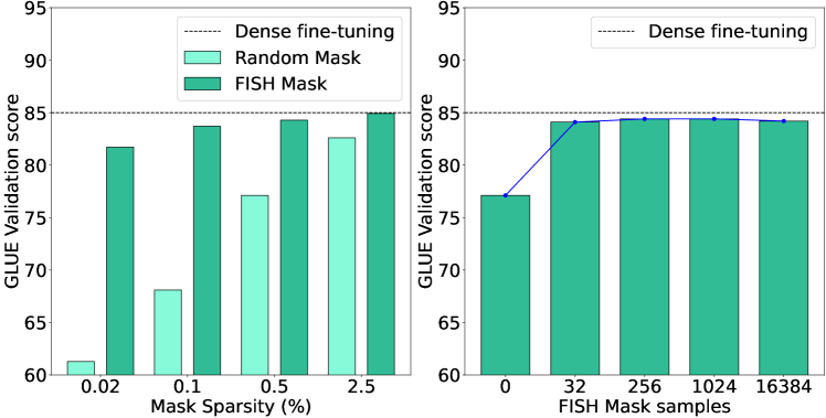
Figure 1: Parameter Samples Scaling Law of FISH Mask

4.1 Intuition

For most of the selective-based PEFT methods, the performance of fine-tuning is related to the scale of the tuned parameters and the size of dataset, which is similar to the scaling-law theory of pretrain language model Kaplan et al. (2020). For FISH Mask, the fine-tuning performance is affected by the parameter scale(Mask Sparsity) and the number of tuning samples, as shown in Fig.1. Once the Mask Sparsity and the set of samples are fixed, FISH mask will select the optimal parameters according to the FIM of the set of samples. However, FISH Mask only focuses on the size of the sample set, and each element in the set is randomly selected. We think that this setting has drawbacks and does not consider the diversity of the samples. When the size of the sample set is determined, selecting better samples to form the set will effectively improve the effect of fine-tuning.

4.2 Data Driven Assumption

In FISH Mask, only the chosen set of parameters $\theta^{*}$ needs to be fine-tuned:

$$\Theta_{0}^{*}=\{\theta_{i}\in\theta|\hat{F}_{\theta_{i}}>={\rm sort}(\hat{F}_{\theta})_{k}\}$$ (4)

The setting of Eq.4 is following Sung et al. (2021), they assume that each training example $x_{i}$ in $\hat{F}_{\theta}$ is independent and identically distributed. In practical datasets, maintaining a consistent data distribution proves challenging, with the presence of considerable noise data making it further complicated. Therefore, there are limitations to random select samples to calculate FIM. In this work, we assume that the samples with larger Fisher-Information (See in Section2.2) are more important in fine-tuning, which will directly affect the quality of parameter selection.

4.3 Iterative Range Decreasing

We propose IRD algorithm to select better samples instead of random selecting. The inputs of IRD algorithm are model $\mathcal{M}$ to be fine-tuned, the set of initial input samples $X_{0}$, and the ground-truth $Y^{*}$. We firstly set variable $l$ to record the iteration and $S$ to receive the output (Step 1). With these inputs, IRD firstly generates the $\Theta_{0}^{*}$, which represents the initial set of parameters with top-k Fisher information (Step 2). Then, the iterative range decreasing process is conducted. During each iteration, if the number of elements in both $X_{l}$ and $\Theta_{l}^{*}$ is greater than one, we alternately halve the range of both $X_{l}$ and $\Theta_{l}^{*}$ (Step 4 and Step 7). And the performance of $\mathcal{M}$ of specific pair of sample-parameter is calculated once the sample or parameter set changes (Step 5 and Step 8). Finally, we get a set of performance scores (calculated by evaluation metrics in Section 5.1) and a corresponding set of tuned parameters.

Input: $X_{0}$; $Y^{*}$;$\mathcal{M}$

Output: $S$

1 $l=0$; $S=\emptyset$;

2$\Theta_{0}^{*}=\{\theta_{i}\in\theta|\hat{F}_{\theta_{i}}>={\rm sort}(\hat{F}_{\theta})_{k}\}$;

3for $|X_{l}|>1$ and $|\Theta_{l}^{*}|>1$ do

4       $X_{l+1}=\{x_{i}\in X_{l}|\hat{F}_{x_{i}}>={\rm sort}(\hat{F}_{x_{i}})_{\frac{|X_{l}|}{2}}\}$;

5      $s={\rm Score}(X_{l+1},Y^{*},\mathcal{M}_{\Theta_{l}^{*}})$;

6      $S=S+\{(s,\Theta_{l}^{*})\}$;

7      $\Theta_{l+1}^{*}=\{\theta_{i}\in\Theta_{l}|\hat{F}_{\theta_{i}}>={\rm sort}(\hat{F}_{\theta})_{\frac{|\Theta_{l}|}{2}}\}$

8      $s={\rm Score}(X_{l+1},Y^{*},\mathcal{M}_{\Theta_{l+1}^{*}})$;

9      $S=S+\{(s,\Theta_{l+1}^{*})\}$;

10      $l=l+1$

11 end for

Algorithm 1 Iterative Range Decreasing

5 Experiments Setup

All experiments can be conducted on a single GPU (RTX-4090-24GB or RTX-8000-48GB) and we mainly work on RTX-4090. Our code framework relies on the PyTorch and Transformer framework.

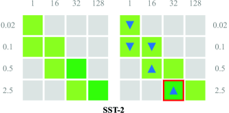
Figure 2: Illustrative compared results on SST-2

FISH Mask on SST-2
Mask	FISH Mask samples
Sparsity	1	16	32	128
0.02	0.9082-
	56881
0.1	0.9128-	0.9105-
	44037	50459
0.5		0.9128-	0.9174-
		44037	31193
2.5			0.9185-	0.9220-
			77982	18349
IRD on SST-2
Mask	FISH Mask samples
Sparsity	1	16	32	128
0.02	0.9071-
	10092 $\downarrow$
0.1	0.9128-	0.9116-
	44037	97248 $\uparrow$
0.5		0.9174-	0.9162-
		31193 $\uparrow$	84404 $\downarrow$
2.5			0.9162-	0.9220-
			84404 $\downarrow$	18349

Table 2: Compared results on SST-2 by BERT

Method	Updated Params	QNLI	SST-2	$\text{MNLI}_{\text{m}}$	$\text{MNLI}_{\text{mm}}$	CoLA	MRPC	STS-B	RTE	QQP
Dense Fine-tuning	100%	93.4	94.9	87.0	86.1	61.0	86.6	86.5	70.9	80.5
Bit-Fit	0.08%	90.4	94.5	85.0	84.8	60.3	86.3	85.0	69.6	78.5
FISH Mask	0.08%	93.3	94.0	85.3	84.9	56.4	86.2	85.7	70.2	79.3
Random Mask	0.50%	89.8	93.4	83.7	84.0	43.2	77.8	87.7	61.3	77.2
Diff Pruning	0.50%	91.9	93.8	86.0	85.5	61.0	86.2	85.6	67.5	80.1
FISH Mask	0.50%	93.1	94.7	86.5	85.9	61.6	87.1	86.5	71.2	80.2
IRD	0.50%	93.3	93.7	86.3	86.6	62.1	90.7	89.9	72.6	88.4
(B)FISH Mask	0.10%	89.9	91.3	79.6	80.4	60.8	88.2	88.4	71.1	85.6
(B)IRD	0.10%	90.4	91.3	82.1	82.4	61.3	88.6	88.8	71.1	86.1
(B)FISH Mask	0.02%	89.4	90.8	73.9	78.1	53.6	88	87.8	66.1	82.8
(B)IRD	0.02%	89.1	90.7	79.1	79.7	54.7	87.9	87.9	69.3	83.9

Table 3: Performance on GLUE. (B) means the foundation model is BERT-base and the default foundation model is BERT-large. Updated Params means the ratio of fine-tuning parameters to all parameters.

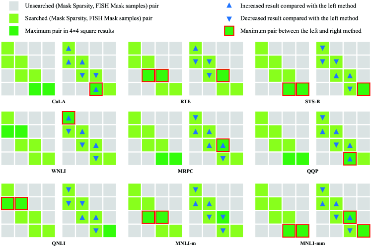
Figure 3: Comparison results between FISH Mask method and IRD-based optimization method on BERT-base

5.1 Datasets and Baselines

Datasets. We evaluate IRD on the GLUEWang et al. (2019) benchmark dataset compared with FISH Mask method. GLUE is a multi-task benchmark that contains 10 tasks for LLMs evaluation. As task AX only has test set for zero-shot learning, we ignore it. We conduct experiments on the original data splits from GLUE.

CoLAWarstadt et al. (2018) is a 2-class classification task of English grammatical acceptability judgments.

SST-2Socher et al. (2013) is a 2-class classification task about human sentiment in movie reviews.

MRPCDolan and Brockett (2005) is a 2-class classification task about senteces pair are semantically equivalent or not.

STS-BCer et al. (2017) is a regression task about sentences pair similarity score from 1.0 to 5.0.

QQP is a 2-class classification task about whether questions pair are semantically equivalent or not.

MNLIWilliams et al. (2018) is a 3-class classification task about the relationship between premise and hypothesis sentences.

QNLIRajpurkar et al. (2016) is a 2-class classification task about the relationship between question and answer.

RTE is a 2-class classification task from annual textual entailment challenges.

WNLILevesque et al. (2012) is a 2-class classification task for predicting whether the original sentence entails the sentence with the pronoun substituted. This task only contains 635 samples for training.

Baselines. Since IRD is based on the selective PEFT method. We choose some selective methods as baselines, including Bit-FitZaken et al. (2022), Diff PruningGuo et al. (2021), original FISH MaskSung et al. (2021). Also, following the settings of Sung et al. (2021), we introduce some simple settings as baselines, such as Dense Fine-tuning and Random Mask. Because the data set and experimental settings are exactly the same, we quoted some experimental results in Sung et al. (2021) and focused on testing IRD and the original FISH Mask method.

5.2 Evaluation Metrics

Evaluation Metrics. The metrics of CoLA task is Matthews correlation coefficientMatthews (1975). The metrics of STS-B task is Pearson and Spearman correlation coefficients. The metrics of MRPC and QQP tasks are combined score(half the sum of the $F_{1}$ and Accuracy). The metrics of other tasks are Accuracy. The settings of evaluation metrics is following Sung et al. (2021).

5.3 Implementation Details

We only use the validation set results as the final results because of the limitation of 2-time uploads to the GLUE official website each day. We follow the same parameter settings for the classification task as BERTDevlin et al. (2019). Apart from the BERT model, we also compare IRD with FISH Mask in the auto-regressive model like GPT-2Radford et al. (2019). We use early stopping to prevent overfit and underfit. The prompt template for GPT-2 is following the Table 1 in Zhong et al. (2023) .

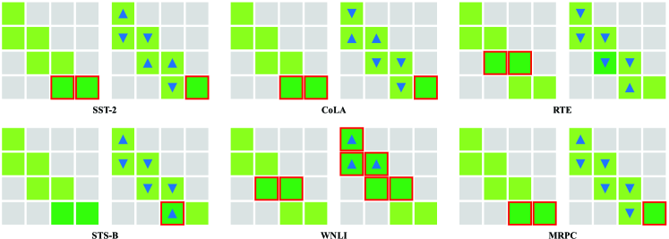
Figure 4: Comparison results between FISH Mask method and IRD-based optimization model on GPT-2

We set different $max\_seq\_length$ for each task in GPT-2, shown in Table4, because of the different maximum sample lengths in different tasks.

Task	max_seq_length
SST-2	128
CoLA	128
RTE	384
STS-B	256
WNLI	128
MRPC	128
QQP	512
QNLI	512
MNLI	512

Table 4: The different setting details in different task for GPT-2.

For the early stopping mechanism, we uses a patience parameter of 10 epochs and a threshold value of 0.3 to determine stopping criteria. Training is halted if there’s no improvement exceeding the patience parameter over 10 consecutive epochs and if the metric value exceeds the threshold value of 0.3. The $learning\_rate$ is 5e-5 in most of the tasks, except WNLI is 5e-6. If the training context only has one sentence, we use "[CLS] sentence I". Otherwise we use "[CLS] sentence I [SEP] sentence II" to concatenate each context. The $batch\_size$ is set to 32. The loss function is cross-entropy and the optimizer is AdamKingma and Ba (2015).

5.4 Experimental Results

We conduct extensive experiments on the GLUE benchmark to verify the effectiveness of the IRD algorithm. Restricted by page limitation, we use pictures instead of specific values, and distinguish the values through color shades and different marks. We will use an example in Section 5.4.1 to show how Table 2 is replaced by Fig.2, and follow this method to draw all experimental results. The remaining numerical values corresponding to illustrated experimental results will be placed in the Appendix.

5.4.1 Case on SST-2 task: An Example

In Fig. 2, we present a comparative visualization of the FISH Mask method versus IRD, which is tested on the SST-2 task using the BERT model. Result of each GLUE task is structured into two 4 by 4 matrices: the one on the left displays the results of the FISH Mask, while the one on the right showcases the results from IRD. Each block within these matrices corresponds to the fine-tuned score of a unique combination of Mask Sparsity and FISH Mask samples, as detailed in Table 2. The varying shades of green color within the cells signify the performance metrics, with darker hues denoting the highest values achieved in each matrix. Besides, the unexplored combinations are indicated by grey blocks.

The lower right corner of the result table and the 4 by 4 matrix both correspond to the original sample-parameter set pair, and are reduced in size in turn through the IRD algorithm. The sample set size decreases from right to left, and the parameter size decreases from bottom to top. Therefore, using the IRD algorithm to search from the lower right corner to the upper left corner will produce a green ladder-like effect that ascends from the lower right to the upper left corner.

Notably, triangles pointing upwards in the right matrix denote outcomes that surpass their counterparts in the left matrix, a relationship mirrored by the arrow indicators in Table2, with downward pointing triangles indicating the opposite. Additionally, the dark green blocks with red borders highlight the overall maximum results across the entire two 4 by 4 matrices layout. Opting for graphical representation over tabular data, we prioritize clarity and efficient space usage in conveying our experimental findings. In experiment, the initial FISH mask sample is 128 and the initial mask sparsity is 2.5 which is set according to the parameter samples scaling law of FISH Mask shown in Fig.1.

5.4.2 Results with BERT on GLUE

Table 3 shows the detailed performance of IRD and baseline methods on the GLUE benchmark. We conducted seven experiments based on BERT-large foundation model. IRD achieves the best performance on 7 out of 9 GLUE subtasks. Besides, under the BERT-base foundation model, IRD achieves the best performance on 6 out of 9 GLUE subtasks.

Fig.3 shows the detailed results of experiments conducted on the GLUE benchmark under BERT-base model, excluding SST-2. Across these tasks, IRD shows better results (more increased arrows than decreased arrows) than the FISH Mask method in CoLA, RTE, STS-B, and MRPC, while it underperforms in WNLI. In QQP, QNLI, MNLI-m, and MNLI-mm, IRD, and FISH Mask call a draw. In conclusion, experimental results prove that the IRD method is better than FISH Mask. There are far more upward arrows than downward arrows (30>22, indicating that IRD is better), which proves the reasonableness and superiority of IRD.

5.4.3 Results with GPT-2 on GLUE

To demonstrate the impact of IRD on the transformer-based decoder-only models, we do experiments on the GPT-2 pre-trained model. Fig. 4 reveals the results of experiments conducted on the GLUE benchmark, using the GPT-2 model. As we have set different $max\_seq\_length$ for each task in GPT-2 that are displayed in Section 5.3, we only run the experiments on six tasks from the GLUE benchmark due to constraints in training time and GPU usage. In SST-2, STS-B, WNLI, and MRPC, IRD achieves better performance than FISH Mask. This result effectively proves the generalizability of IRD under different foundation models.

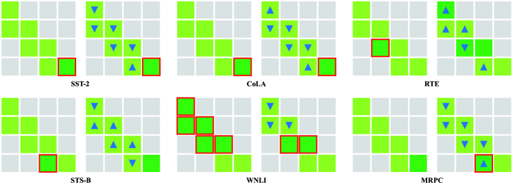
Figure 5: Contrastive Study

5.4.4 Contrastive Study

To demonstrate the enhancement of IRD over the FISH Mask method, we switch the sample choosing step (Step 4) and parameter choosing step(Step 7) of Algorithm1 to a contrastive way, aiming for inverse results. In Algorithm1, Step 4 represents selecting the larger half of elements from set $X_{l}$ to form a new set. Here, we modify it to select the larger half of elements from set $X_{l}$, but this time from the latter half (Shown in Eq.5). In Eq.6, we make the same operation for the set of $\Theta_{l}^{*}$.

$$X_{l+1}=\{x_{i}\in X_{l}|\hat{F}_{x_{i}}<{\rm sort}(\hat{F}_{x_{i}})_{\frac{|X_{l}|}{2}}\}$$ (5)

$$\Theta_{l+1}^{*}=\{\theta_{i}\in\Theta_{l}|\hat{F}_{\theta_{i}}<{\rm sort}(\hat{F}_{\theta})_{\frac{|\Theta_{l}|}{2}}\}$$ (6)

Fig.5 reveals the results of experiments conducted on the GLUE dataset, using the GPT-2 model. As shown in Fig.5, the result on each GLUE task is structured into two 4 by 4 matrices: the one on the left displays the results of IRD, while the one on the right showcases the results from the contrastive method.

In non-tie results, IRD is better than Fish-mask. We can see the obvious advantages of IRD from Fig.4. We set IRD to search in the opposite direction of optimization, that is, search for worse values in each iteration, and put the results on the right, and IRD on the left for comparison in Fig.4. Experimental results prove that the IRD method is better than reverse IRD on four subtasks. There are far more downward arrows than upward arrows (20>12, indicating that reverse IRD reduces performance), which proves the reasonableness and superiority of IRD search.

Across these six tasks, the modified algorithm shows more improvements (more increased arrows than decreased arrows) than IRD in RTE, STS-B, while it underperforms in SST-2, CoLA, WNLI, and MRPC. Regarding the overall results in the two matrices, the modified algorithm achieves the highest results in MRPC. IRD outperforms the modified algorithm in RTE and STS-B, while both methods tie for the highest results in SST-2, CoLA, and WNLI.

5.5 Analysis

In this work, we design different types of experiments to evaluate IRD algorithm. The chosen GLUE benchmark can fully verify the generalization of the model and facilitate comparison with other methods. By thoroughly compared with the mainstream selective-based PEFT method without changing the dataset is sufficient to demonstrate the effectiveness of our method. Besides, comparing with FISH-Mask under different foundation models further demonstrates our method’s efficacy. A contrastive study shows our method has improved on more corresponding squares and also achieved optimal values on more tasks. These results demonstrate IRD is an effective optimization algorithm because the reverse settings get worse results.

It is worth noting that when the optimal result (red border square) appears in the lower right corner of the 4 by 4 matrix, it means that the model has achieved the best result on the initial sample-parameter size. In this case, the FISH-Mask method and the IRD algorithm get in a draw. This is because the optimal sample-parameter pair appears outside the initial range, and the IRD algorithm cannot achieve better results by continuing to decrease the sample-parameter range.

6 Conclusion

In this paper, we adopt a data-oriented perspective to optimize PEFT method before training. Based on this methodology, we propose IRD algorithm to optimize FISH Mask based method. Besides, we designed and conducted experiments to verify the effectiveness of the proposed algorithm, and the experimental results also verified our methodology. We hope our efforts can inspire research in related fields, directing more attention towards data-driven PEFT methods. In future work, we will explore a set of general data-oriented PEFT optimization algorithms instead of just optimizing a certain model. In addition, we will try and explore the relationship between PEFT method data and parameters more deeply.

Limitations

Although we proposed a general data-oriented PEFT method optimization idea, the algorithm we designed only optimizes a specific model. Furthermore, IRD cannot dynamically adjust the model during training, and all settings are determined before training. Both of these limitations can be further optimized in subsequent work.

Ethics Statement

In this study on parameter efficient fine tuning using the GLUE benchmark and pre-trained models like BERT or GPT-2, we recognize the importance of ethical considerations in our methodology and findings. Acknowledging that the datasets and models employed may inherently carry biases reflective of their training sources, we are mindful of the potential for misuse or misinterpretation in sensitive applications. We advocate for the responsible application of our findings, emphasizing the importance of ethical usage to avoid social harm.

We have ensured the transparency and reproducibility of our research by making our code and methodologies publicly available. This is in line with our commitment to fostering trust and integrity in natural language processing research.

Appendix A Tables of Precision Results

FISH Mask on CoLA
Mask	FISH Mask samples
Sparsity	1	16	32	128
0.02	0.5364-
	12896
0.1	0.6083-	0.5942-
	70776	58898
0.5		0.6196-	0.6137-
		50422	21879
2.5			0.6211-	0.6120-
			92519	85127
IRD on CoLA
Mask	FISH Mask samples
Sparsity	1	16	32	128
0.02	0.5469-
	58705 $\uparrow$
0.1	0.6132-	0.6132-
	37959 $\uparrow$	37959 $\uparrow$
0.5		0.6194-	0.6240-
		38412 $\downarrow$	83897 $\uparrow$
2.5			0.6162-	0.6120-
			36749 $\downarrow$	85127

Table 5: Compared results on CoLA by BERT

FISH Mask on RTE
Mask	FISH Mask samples
Sparsity	1	16	32	128
0.02	0.6606-
	49819
0.1	0.7111-	0.7400-
	91336	72202
0.5		0.7364-	0.7364-
		62094	62094
2.5			0.7148-	0.7148-
			01444	01444
IRD on RTE
Mask	FISH Mask samples
Sparsity	1	16	32	128
0.02	0.6931-
	40794 $\uparrow$
0.1	0.7111-	0.7111-
	91336	91336 $\downarrow$
0.5		0.7509-	0.7400-
		02527 $\uparrow$	72202 $\uparrow$
2.5			0.7328-	0.7148-
			51986 $\uparrow$	01444

Table 6: Compared results on RTE by BERT

FISH Mask on STS-B
Mask	FISH Mask samples
Sparsity	1	16	32	128
0.02	0.8784-
	29404
0.1	0.8843-	0.8874-
	99414	82622
0.5		0.8904-	0.8899-
		70230	26925
2.5			0.8930-	0.8966-
			60770	27263
IRD on STS-B
Mask	FISH Mask samples
Sparsity	1	16	32	128
0.02	0.8788-
	92200 $\uparrow$
0.1	0.8876-	0.8875-
	48950 $\uparrow$	52835 $\uparrow$
0.5		0.8920-	0.8921-
		09119 $\uparrow$	15572 $\uparrow$
2.5			0.8968-	0.8966-
			80132 $\uparrow$	27263

Table 7: Compared results on STS-B by BERT

FISH Mask on WNLI
Mask	FISH Mask samples
Sparsity	1	16	32	128
0.02	0.5774-
	64789
0.1	0.5633-	0.5774-
	80282	64789
0.5		0.5915-	0.5915-
		49296	49296
2.5			0.5211-	0.5070-
			26761	42254
IRD on WNLI
Mask	FISH Mask samples
Sparsity	1	16	32	128
0.02	0.5633-
	80282 $\downarrow$
0.1	0.5633-	0.5633-
	80282	80282 $\downarrow$
0.5		0.5633-	0.5633-
		80282 $\downarrow$	80282 $\downarrow$
2.5			0.5070-	0.5070-
			42254 $\downarrow$	42254

Table 8: Compared results on WNLI by BERT

FISH Mask on MRPC
Mask	FISH Mask samples
Sparsity	1	16	32	128
0.02	0.8800-
	59185
0.1	0.8817-	0.8950-
	27159	19196
0.5		0.8869-	0.8825-
		48529	92061
2.5			0.8747-	0.8866-
			46450	20732
IRD on MRPC
Mask	FISH Mask samples
Sparsity	1	16	32	128
0.02	0.8787-
	48558 $\downarrow$
0.1	0.8862-	0.8864-
	88318 $\uparrow$	55108 $\downarrow$
0.5		0.8874-	0.8834-
		31777 $\uparrow$	27344 $\uparrow$
2.5			0.8785-	0.8866-
			74346 $\uparrow$	20732

Table 9: Compared results on MRPC by BERT

FISH Mask on QQP
Mask	FISH Mask samples
Sparsity	1	16	32	128
0.02	0.8279-
	72035
0.1	0.8562-	0.8630-
	98482	70508
0.5		0.8766-	0.8771-
		64736	79970
2.5			0.8847-	0.8873-
			38135	17030
IRD on QQP
Mask	FISH Mask samples
Sparsity	1	16	32	128
0.02	0.8386-
	33700 $\uparrow$
0.1	0.8616-	0.8616-
	14642 $\uparrow$	14642 $\downarrow$
0.5		0.8820-	0.8768-
		65026 $\uparrow$	32596 $\downarrow$
2.5			0.8845-	0.8873-
			00562 $\downarrow$	17030

Table 10: Compared results on QQP by BERT

FISH Mask on QNLI
Mask	FISH Mask samples
Sparsity	1	16	32	128
0.02	0.8943-
	80377
0.1	0.8993-	0.9059-
	22716	12502
0.5		0.9081-	0.9062-
		09098	78602
2.5			0.9086-	0.9084-
			58246	75197
IRD on QNLI
Mask	FISH Mask samples
Sparsity	1	16	32	128
0.02	0.8909-
	02435 $\downarrow$
0.1	0.9048-	0.9040-
	14205 $\uparrow$	82006 $\downarrow$
0.5		0.9070-	0.9075-
		10800 $\downarrow$	59949 $\uparrow$
2.5			0.9117-	0.9084-
			70090 $\uparrow$	75197

Table 11: Compared results on QNLI by BERT

FISH Mask on MNLI-m
Mask	FISH Mask samples
Sparsity	1	16	32	128
0.02	0.7388-
	69078
0.1	0.7963-	0.8159-
	32145	95925
0.5		0.8295-	0.8300-
		46612	56037
2.5			0.8382-	0.8347-
			06826	42741
IRD on MNLI-m
Mask	FISH Mask samples
Sparsity	1	16	32	128
0.02	0.7909-
	32247 $\uparrow$
0.1	0.8207-	0.8207-
	84513 $\uparrow$	84513 $\uparrow$
0.5		0.8268-	0.8255-
		97606 $\downarrow$	73102 $\downarrow$
2.5			0.8368-	0.8347-
			82323 $\downarrow$	42741

Table 12: Compared results on MNLI-m by BERT

FISH Mask on MNLI-mm
Mask	FISH Mask samples
Sparsity	1	16	32	128
0.02	0.7506-
	10252
0.1	0.8041-	0.8189-
	09032	58503
0.5		0.8251-	0.8341-
		62734	13100
2.5			0.8347-	0.8359-
			23352	43857
IRD on MNLI-mm
Mask	FISH Mask samples
Sparsity	1	16	32	128
0.02	0.7967-
	86005 $\uparrow$
0.1	0.8240-	0.8197-
	43938 $\uparrow$	72172 $\uparrow$
0.5		0.8227-	0.8215-
		21725 $\downarrow$	01221 $\downarrow$
2.5			0.8327-	0.8359-
			90887 $\downarrow$	43857

Table 13: Compared results on MNLI-mm by BERT

FISH Mask on SST-2
Mask	FISH Mask samples
Sparsity	1	16	32	128
0.02	0.9071-
	10092
0.1	0.9139-	0.9151-
	90826	37615
0.5		0.9139-	0.9139-
		90826	90826
2.5			0.9139-	0.9139-
			90826	90826
IRD on SST-2
Mask	FISH Mask samples
Sparsity	1	16	32	128
0.02	0.9071-
	10092
0.1	0.9082-	0.9094-
	56881 $\downarrow$	03670 $\downarrow$
0.5		0.9162-	0.9162-
		84404 $\uparrow$	84404 $\uparrow$
2.5			0.9128-	0.9139-
			44037 $\downarrow$	90826

Table 14: Compared results on SST-2 by GPT-2

FISH Mask on CoLA
Mask	FISH Mask samples
Sparsity	1	16	32	128
0.02	0.4411-
	21566
0.1	0.4608-	0.5203-
	37120	12159
0.5		0.5469-	0.5656-
		07507	29691
2.5			0.5422-	0.5176-
			27824	61792
IRD on CoLA
Mask	FISH Mask samples
Sparsity	1	16	32	128
0.02	0.4471-
	42466 $\uparrow$
0.1	0.5111-	0.5111-
	15462 $\uparrow$	15462 $\downarrow$
0.5		0.5282-	0.5353-
		40425 $\downarrow$	92581 $\downarrow$
2.5			0.5294-	0.5176-
			39529 $\downarrow$	61792

Table 15: Compared results on CoLA by GPT-2

FISH Mask on RTE
Mask	FISH Mask samples
Sparsity	1	16	32	128
0.02	0.6859-
	20578
0.1	0.6750-	0.6931-
	90253	40794
0.5		0.6895-	0.6750-
		30686	90253
2.5			0.6787-	0.6606-
			00361	49819
IRD on RTE
Mask	FISH Mask samples
Sparsity	1	16	32	128
0.02	0.6859-
	20578
0.1	0.6895-	0.6895-
	30686 $\uparrow$	30686 $\downarrow$
0.5		0.6859-	0.6678-
		20578 $\downarrow$	70036 $\downarrow$
2.5			0.6642-	0.6606-
			59928 $\downarrow$	49819

Table 16: Compared results on RTE by GPT-2

FISH Mask on STS-B
Mask	FISH Mask samples
Sparsity	1	16	32	128
0.02	0.8628-
	15696
0.1	0.8726-	0.8733-
	16696	94962
0.5		0.8707-	0.8714-
		61240	91968
2.5			0.8741-	0.8778-
			62863	00614
IRD on STS-B
Mask	FISH Mask samples
Sparsity	1	16	32	128
0.02	0.8638-
	74896 $\uparrow$
0.1	0.8727-	0.8727-
	16163 $\uparrow$	13879 $\downarrow$
0.5		0.8721-	0.8721-
		18050 $\uparrow$	98328 $\uparrow$
2.5			0.8774-	0.8778-
			09002 $\uparrow$	00614

Table 17: Compared results on STS-B by GPT-2

FISH Mask on WNLI
Mask	FISH Mask samples
Sparsity	1	16	32	128
0.02	0.5633-
	80282
0.1	0.6056-	0.5774-
	33803	64789
0.5		0.6056-	0.6056-
		33803	33803
2.5			0.6056-	0.6197-
			33803	18310
IRD on WNLI
Mask	FISH Mask samples
Sparsity	1	16	32	128
0.02	0.5915-
	49296 $\uparrow$
0.1	0.5915-	0.5915-
	49296 $\downarrow$	49296 $\uparrow$
0.5		0.6056-	0.6056-
		33803	33803
2.5			0.6197-	0.6197-
			18310 $\uparrow$	18310

Table 18: Compared results on WNLI by GPT-2

FISH Mask on MRPC
Mask	FISH Mask samples
Sparsity	1	16	32	128
0.02	0.8308-
	04639
0.1	0.8387-	0.8554-
	55199	90854
0.5		0.8487-	0.8484-
		79486	58462
2.5			0.8647-	0.8580-
			87582	36850
IRD on MRPC
Mask	FISH Mask samples
Sparsity	1	16	32	128
0.02	0.8226-
	50646 $\downarrow$
0.1	0.8556-	0.8556-
	49149 $\uparrow$	49149 $\uparrow$
0.5		0.8498-	0.8487-
		07103 $\uparrow$	79486 $\uparrow$
2.5			0.8741-	0.8580-
			56321 $\uparrow$	36850

Table 19: Compared results on MRPC by GPT-2

IRD on SST-2
Mask	FISH Mask samples
Sparsity	1	16	32	128
0.02	0.9116-
	97248
0.1	0.9105-	0.9094-
	50459	03670
0.5		0.9162-	0.9162-
		84404	84404
2.5			0.9162-	0.9197-
			84404	24771
IRD-inverse on SST-2
Mask	FISH Mask samples
Sparsity	1	16	32	128
0.02	0.9013-
	76147 $\downarrow$
0.1	0.9071-	0.9071-
	10092 $\downarrow$	10092 $\downarrow$
0.5		0.9151-	0.9151-
		37615 $\downarrow$	37615 $\downarrow$
2.5			0.9174-	0.9197-
			31193 $\uparrow$	24771

Table 20: Contrastive Study on SST-2 by GPT-2

IRD on CoLA
Mask	FISH Mask samples
Sparsity	1	16	32	128
0.02	0.4260-
	24490
0.1	0.5241-	0.5241-
	75362	75362
0.5		0.5235-	0.5258-
		22165	66331
2.5			0.5312-	0.5365-
			01720	00716
IRD-inverse on CoLA
Mask	FISH Mask samples
Sparsity	1	16	32	128
0.02	0.4440-
	81207 $\uparrow$
0.1	0.4758-	0.4758-
	82812 $\downarrow$	82812 $\downarrow$
0.5		0.5206-	0.5206-
		02684 $\downarrow$	02684 $\downarrow$
2.5			0.5312-	0.5365-
			51877 $\uparrow$	00716

Table 21: Contrastive Study on CoLA by GPT-2

IRD on RTE
Mask	FISH Mask samples
Sparsity	1	16	32	128
0.02	0.6787-
	00361
0.1	0.6750-	0.6750-
	90253	90253
0.5		0.6895-	0.6859-
		30686	20578
2.5			0.6750-	0.6714-
			90253	80144
IRD-inverse on RTE
Mask	FISH Mask samples
Sparsity	1	16	32	128
0.02	0.6859-
	20578 $\uparrow$
0.1	0.6823-	0.6823-
	10469 $\uparrow$	10469 $\uparrow$
0.5		0.6859-	0.6859-
		20578 $\downarrow$	20578
2.5			0.6823-	0.6714-
			10469 $\uparrow$	80144

Table 22: Contrastive Study on RTE by GPT-2

IRD on STS-B
Mask	FISH Mask samples
Sparsity	1	16	32	128
0.02	0.8634-
	49302
0.1	0.8677-	0.8678-
	95376	00566
0.5		0.8679-	0.8680-
		89910	01243
2.5			0.8706-	0.8702-
			74675	57955
IRD-inverse on STS-B
Mask	FISH Mask samples
Sparsity	1	16	32	128
0.02	0.8611-
	47175 $\downarrow$
0.1	0.8684-	0.8684-
	53074 $\uparrow$	55518 $\uparrow$
0.5		0.8695-	0.8693-
		07693 $\uparrow$	85954 $\uparrow$
2.5			0.8689-	0.8702-
			25294 $\downarrow$	57955

Table 23: Contrastive Study on STS-B by GPT-2

IRD on WNLI
Mask	FISH Mask samples
Sparsity	1	16	32	128
0.02	0.6056-
	33803
0.1	0.6056-	0.6056-
	33803	33803
0.5		0.6056-	0.6056-
		33803	33803
2.5			0.5774-	0.5774-
			64789	64789
IRD-inverse on WNLI
Mask	FISH Mask samples
Sparsity	1	16	32	128
0.02	0.5915-
	49296 $\downarrow$
0.1	0.5915-	0.5915-
	49296 $\downarrow$	49296 $\downarrow$
0.5		0.6056-	0.6056-
		33803	33803
2.5			0.5774-	0.5774-
			64789	64789

Table 24: Contrastive Study on WNLI by GPT-2

IRD on MRPC
Mask	FISH Mask samples
Sparsity	1	16	32	128
0.02	0.8478-
	51931
0.1	0.8389-	0.8389-
	75523	75523
0.5		0.8510-	0.8510-
		35571	35571
2.5			0.8531-	0.8594-
			32784	27609
IRD-inverse on MRPC
Mask	FISH Mask samples
Sparsity	1	16	32	128
0.02	0.8404-
	77338 $\downarrow$
0.1	0.8374-	0.8374-
	62481 $\downarrow$	62481 $\downarrow$
0.5		0.8498-	0.8498-
		07103 $\downarrow$	07103 $\downarrow$
2.5			0.8651-	0.8594-
			64869 $\uparrow$	27609

Table 25: Contrastive Study on MRPC by GPT-2

References

- Amari (1996) Shun-ichi Amari. 1996. Neural learning in structured parameter spaces-natural riemannian gradient. Advances in neural information processing systems, 9.
- Arora et al. (2018) Sanjeev Arora, Rong Ge, Behnam Neyshabur, and Yi Zhang. 2018. Stronger generalization bounds for deep nets via a compression approach. In ICML, volume 80 of Proceedings of Machine Learning Research, pages 254–263. PMLR.
- Brown et al. (2020) Tom B. Brown, Benjamin Mann, Nick Ryder, Melanie Subbiah, Jared Kaplan, Prafulla Dhariwal, Arvind Neelakantan, Pranav Shyam, Girish Sastry, Amanda Askell, Sandhini Agarwal, Ariel Herbert-Voss, Gretchen Krueger, Tom Henighan, Rewon Child, Aditya Ramesh, Daniel M. Ziegler, Jeffrey Wu, Clemens Winter, Christopher Hesse, Mark Chen, Eric Sigler, Mateusz Litwin, Scott Gray, Benjamin Chess, Jack Clark, Christopher Berner, Sam McCandlish, Alec Radford, Ilya Sutskever, and Dario Amodei. 2020. Language models are few-shot learners. In NeurIPS.
- Cer et al. (2017) Daniel M. Cer, Mona T. Diab, Eneko Agirre, Iñigo Lopez-Gazpio, and Lucia Specia. 2017. Semeval-2017 task 1: Semantic textual similarity - multilingual and cross-lingual focused evaluation. CoRR, abs/1708.00055.
- Devlin et al. (2019) Jacob Devlin, Ming-Wei Chang, Kenton Lee, and Kristina Toutanova. 2019. BERT: pre-training of deep bidirectional transformers for language understanding. In NAACL-HLT (1), pages 4171–4186. Association for Computational Linguistics.
- Ding et al. (2023a) Ning Ding, Xingtai Lv, Qiaosen Wang, Yulin Chen, Bowen Zhou, Zhiyuan Liu, and Maosong Sun. 2023a. Sparse low-rank adaptation of pre-trained language models. CoRR, abs/2311.11696.
- Ding et al. (2023b) Ning Ding, Yujia Qin, Guang Yang, Fuchao Wei, Zonghan Yang, Yusheng Su, Shengding Hu, Yulin Chen, Chi-Min Chan, Weize Chen, Jing Yi, Weilin Zhao, Xiaozhi Wang, Zhiyuan Liu, Hai-Tao Zheng, Jianfei Chen, Yang Liu, Jie Tang, Juanzi Li, and Maosong Sun. 2023b. Parameter-efficient fine-tuning of large-scale pre-trained language models. Nat. Mac. Intell., 5(3):220–235.
- Dolan and Brockett (2005) William B. Dolan and Chris Brockett. 2005. Automatically constructing a corpus of sentential paraphrases. In IWP@IJCNLP. Asian Federation of Natural Language Processing.
- Fisher (1922) Ronald A Fisher. 1922. On the mathematical foundations of theoretical statistics. Philosophical transactions of the Royal Society of London. Series A, containing papers of a mathematical or physical character, 222(594-604):309–368.
- French (1999) Robert M French. 1999. Catastrophic forgetting in connectionist networks. Trends in cognitive sciences, 3(4):128–135.
- Guo et al. (2021) Demi Guo, Alexander M. Rush, and Yoon Kim. 2021. Parameter-efficient transfer learning with diff pruning. In ACL/IJCNLP (1), pages 4884–4896. Association for Computational Linguistics.
- Houlsby et al. (2019) Neil Houlsby, Andrei Giurgiu, Stanislaw Jastrzebski, Bruna Morrone, Quentin de Laroussilhe, Andrea Gesmundo, Mona Attariyan, and Sylvain Gelly. 2019. Parameter-efficient transfer learning for NLP. In ICML, volume 97 of Proceedings of Machine Learning Research, pages 2790–2799. PMLR.
- Hu et al. (2022) Edward J. Hu, Yelong Shen, Phillip Wallis, Zeyuan Allen-Zhu, Yuanzhi Li, Shean Wang, Lu Wang, and Weizhu Chen. 2022. Lora: Low-rank adaptation of large language models. In ICLR. OpenReview.net.
- Kaplan et al. (2020) Jared Kaplan, Sam McCandlish, Tom Henighan, Tom B. Brown, Benjamin Chess, Rewon Child, Scott Gray, Alec Radford, Jeffrey Wu, and Dario Amodei. 2020. Scaling laws for neural language models. CoRR, abs/2001.08361.
- Kingma and Ba (2015) Diederik P. Kingma and Jimmy Ba. 2015. Adam: A method for stochastic optimization. In ICLR (Poster).
- Levesque et al. (2012) Hector J. Levesque, Ernest Davis, and Leora Morgenstern. 2012. The winograd schema challenge. In KR. AAAI Press.
- Li et al. (2018) Chunyuan Li, Heerad Farkhoor, Rosanne Liu, and Jason Yosinski. 2018. Measuring the intrinsic dimension of objective landscapes. In ICLR (Poster). OpenReview.net.
- Lialin et al. (2023) Vladislav Lialin, Vijeta Deshpande, and Anna Rumshisky. 2023. Scaling down to scale up: A guide to parameter-efficient fine-tuning. CoRR, abs/2303.15647.
- Liu et al. (2022a) Haokun Liu, Derek Tam, Mohammed Muqeeth, Jay Mohta, Tenghao Huang, Mohit Bansal, and Colin Raffel. 2022a. Few-shot parameter-efficient fine-tuning is better and cheaper than in-context learning. In NeurIPS.
- Liu et al. (2022b) Xiao Liu, Kaixuan Ji, Yicheng Fu, Weng Tam, Zhengxiao Du, Zhilin Yang, and Jie Tang. 2022b. P-tuning: Prompt tuning can be comparable to fine-tuning across scales and tasks. In ACL (2), pages 61–68. Association for Computational Linguistics.
- Maddox et al. (2020) Wesley J. Maddox, Gregory W. Benton, and Andrew Gordon Wilson. 2020. Rethinking parameter counting in deep models: Effective dimensionality revisited. CoRR, abs/2003.02139.
- Malladi et al. (2023) Sadhika Malladi, Alexander Wettig, Dingli Yu, Danqi Chen, and Sanjeev Arora. 2023. A kernel-based view of language model fine-tuning. In ICML, volume 202 of Proceedings of Machine Learning Research, pages 23610–23641. PMLR.
- Matthews (1975) Brian W Matthews. 1975. Comparison of the predicted and observed secondary structure of t4 phage lysozyme. Biochimica et Biophysica Acta (BBA)-Protein Structure, 405(2):442–451.
- McClelland et al. (1995) James L McClelland, Bruce L McNaughton, and Randall C O’Reilly. 1995. Why there are complementary learning systems in the hippocampus and neocortex: insights from the successes and failures of connectionist models of learning and memory. Psychological review, 102(3):419.
- McCloskey and Cohen (1989) Michael McCloskey and Neal J Cohen. 1989. Catastrophic interference in connectionist networks: The sequential learning problem. In Psychology of learning and motivation, volume 24, pages 109–165. Elsevier.
- Pascanu and Bengio (2014) Razvan Pascanu and Yoshua Bengio. 2014. Revisiting natural gradient for deep networks. In ICLR.
- Radford et al. (2019) Alec Radford, Jeffrey Wu, Rewon Child, David Luan, Dario Amodei, Ilya Sutskever, et al. 2019. Language models are unsupervised multitask learners. OpenAI blog, 1(8):9.
- Rajpurkar et al. (2016) Pranav Rajpurkar, Jian Zhang, Konstantin Lopyrev, and Percy Liang. 2016. Squad: 100, 000+ questions for machine comprehension of text. In EMNLP, pages 2383–2392. The Association for Computational Linguistics.
- Ratcliff (1990) Roger Ratcliff. 1990. Connectionist models of recognition memory: constraints imposed by learning and forgetting functions. Psychological review, 97(2):285.
- Socher et al. (2013) Richard Socher, Alex Perelygin, Jean Wu, Jason Chuang, Christopher D. Manning, Andrew Y. Ng, and Christopher Potts. 2013. Recursive deep models for semantic compositionality over a sentiment treebank. In EMNLP, pages 1631–1642. ACL.
- Sung et al. (2021) Yi-Lin Sung, Varun Nair, and Colin Raffel. 2021. Training neural networks with fixed sparse masks. In NeurIPS, pages 24193–24205.
- Valipour et al. (2023) Mojtaba Valipour, Mehdi Rezagholizadeh, Ivan Kobyzev, and Ali Ghodsi. 2023. Dylora: Parameter-efficient tuning of pre-trained models using dynamic search-free low-rank adaptation. In EACL, pages 3266–3279. Association for Computational Linguistics.
- Wang et al. (2019) Alex Wang, Amanpreet Singh, Julian Michael, Felix Hill, Omer Levy, and Samuel R. Bowman. 2019. GLUE: A multi-task benchmark and analysis platform for natural language understanding. In ICLR (Poster). OpenReview.net.
- Warstadt et al. (2018) Alex Warstadt, Amanpreet Singh, and Samuel R. Bowman. 2018. Neural network acceptability judgments. CoRR, abs/1805.12471.
- Williams et al. (2018) Adina Williams, Nikita Nangia, and Samuel R. Bowman. 2018. A broad-coverage challenge corpus for sentence understanding through inference. In NAACL-HLT, pages 1112–1122. Association for Computational Linguistics.
- Zaken et al. (2022) Elad Ben Zaken, Yoav Goldberg, and Shauli Ravfogel. 2022. Bitfit: Simple parameter-efficient fine-tuning for transformer-based masked language-models. In ACL (2), pages 1–9. Association for Computational Linguistics.
- Zhao et al. (2020) Mengjie Zhao, Tao Lin, Fei Mi, Martin Jaggi, and Hinrich Schütze. 2020. Masking as an efficient alternative to finetuning for pretrained language models. In EMNLP (1), pages 2226–2241. Association for Computational Linguistics.
- Zhong et al. (2023) Qihuang Zhong, Liang Ding, Juhua Liu, Bo Du, and Dacheng Tao. 2023. Can chatgpt understand too? A comparative study on chatgpt and fine-tuned BERT. CoRR, abs/2302.10198.