Authorship Verification based on
the Likelihood Ratio of Grammar Models

Abstract

Authorship verification (AV) is the process of analyzing a set of documents to determine whether they were written by a specific author. This problem often arises in forensic scenarios, e.g., in cases where the documents in question constitute evidence for a crime. Existing state-of-the-art AV methods use computational solutions that are not supported by a plausible scientific explanation for their functioning and that are often difficult for analysts to interpret. To address this, we propose a method relying on calculating a quantity we call $\lambda_{G}$ (LambdaG): the ratio between the likelihood of a document given a model of the Grammar for the candidate author and the likelihood of the same document given a model of the Grammar for a reference population. These Grammar Models are estimated using $n$-gram language models that are trained solely on grammatical features. Despite not needing large amounts of data for training, LambdaG still outperforms other established AV methods with higher computational complexity, including a fine-tuned Siamese Transformer network. Our empirical evaluation based on four baseline methods applied to twelve datasets shows that LambdaG leads to better results in terms of both accuracy and AUC in eleven cases and in all twelve cases if considering only topic-agnostic methods. The algorithm is also highly robust to important variations in the genre of the reference population in many cross-genre comparisons. In addition to these properties, we demonstrate how LambdaG is easier to interpret than the current state-of-the-art. We argue that the advantage of LambdaG over other methods is due to fact that it is compatible with Cognitive Linguistic theories of language processing.

1 Introduction

Texts serve numerous purposes and can be found in a variety of digital and non-digital forms such as books, social media posts, emails, letters, websites, academic papers, blogs, product reviews, poems and many others. These text types, in turn, can be categorized according to various criteria including language, genre, topic, readability or authorship. The latter is particularly important when it comes to investigating questioned documents, for example, in forensic settings, e. g., blackmail letters, suicide notes, letters of confession, wills or theses potentially written by ghostwriters.

Over the course of time, various research disciplines have emerged to deal with the analysis of the language of authors from different perspectives. This has led to an interdisciplinary branch of research that is often referred to as digital text forensics in the literature (e. g., [90, 10, 40, 95, 38]). Two well-known and closely related sub-areas of this branch of research are authorship attribution (AA) and authorship verification (AV). AA is concerned with the task of attributing an anonymous text to the most likely author based on a set of sample documents of known authors. AV, on the other hand, deals (in its simplest form) with the task of deciding whether two documents were written by the same author. Our focus in this paper is on AV, which represents a reformulation of AA, based on the fact that any AA problem can be decomposed into a series of AV problems [67].

1.1 Decision Problems

According to Stein et al. [105], Juola and Stamatatos [55], Koppel et al. [67] and Halvani [41] the following decision problems can be answered by AV:

1. $\textrm{AV}_{\,\textrm{Core}}$: Given two documents $\mathcal{D}_{1}$ and $\mathcal{D}_{2}$: Were both documents written by the same author?

2. $\textrm{AV}_{\,\textrm{Batch}}$: Given two sets of documents $\mathbb{D}_{\mathcal{A}}=\{\mathcal{D}^{\,(a)}_{1},\mathcal{D}^{\,(a)}_{2},\ldots\}$ and $\mathbb{D}_{\mathcal{B}}=\{\mathcal{D}^{\,(b)}_{1},\mathcal{D}^{\,(b)}_{2},\ldots\}$ each of which written by a single author: Are the documents in $\mathbb{D}_{\mathcal{A}}$ and $\mathbb{D}_{\mathcal{B}}$ written by the same author?

3. $\textrm{AV}_{\,\textrm{Known}}$: Given a set of documents $\mathbb{D}_{\mathcal{A}}=\{\mathcal{D}_{1},\mathcal{D}_{2},\ldots\}$ by the same author $\mathcal{A}$ as well as a document $\mathcal{D}_{\mathcal{U}}$ of an unknown author $\mathcal{U}$: Has $\mathcal{A}$ also written $\mathcal{D}_{\mathcal{U}}$ such that $\mathcal{A}=\mathcal{U}$ holds?

In a forensic context the process of assisting the trier-of-facts in finding answers to these problems is referred to as Forensic Text Comparison (FTC) [49]. The focus in this paper is on all three of these decisions problems. For the rest of this paper, we adopt the following notation: a document denoted by $\mathcal{D}_{\mathcal{U}}$, represents a document of an unknown author $\mathcal{U}$, whereas a document denoted by $\mathcal{D}_{\mathcal{A}}$ represents a document of a known author $\mathcal{A}$. In all decision problems, including $\textrm{AV}_{\,\textrm{Core}}$ where the denotation of which document is known or unknown can be arbitrary, an AV method seeks to answer the question of whether $\mathcal{A}=\mathcal{U}$ ($\mathcal{A}$ authored $\mathcal{D}_{\mathcal{U}}$) or $\mathcal{A}\neq\mathcal{U}$ ($\mathcal{A}$ did not author $\mathcal{D}_{\mathcal{U}}$) holds. In this context, a known verification case with a matching and non-matching authorship is denoted by Y- and N-case, respectively. Moreover, we denote $\neg\mathcal{A}$ as any author other than $\mathcal{A}$.

1.2 Applications of Authorship Verification

For all the mentioned forms of decision problems, numerous AV applications can be found across different domains. In forensic linguistics, for example, AV can be used to analyze malicious texts such as ransom notes, blackmail letters or other non-malicious texts that are used as evidence in investigatory, criminal or civil contexts. In the field of journalism and media, AV can play a vital role when it comes to confirming the authorship of news articles or opinion pieces or investigating cases of ghostwriting and unauthorized publication of content. In academia, AV can be used to analyze research articles, dissertations or other written content, for example, to resolve a plagiarism claim, or contract cheating from students, and thereby overall contribute to combating academic misconduct. In the context of social media, AV can also be employed to detect fake accounts or multiple accounts belonging to the same user. Moreover, as part of email and communication analysis, AV can be used to verify the authorship of emails in cases of fraud, harassment or cybercrime. Finally, in the Digital Humanities, AV can be used to resolve matters that deal with disputed historical evidence or to provide evidence in favour or against the origin of literary works.

1.3 Categories of AV Methods

According to Halvani et al. [43, 47], AV methods can be divided into three possible categories, namely unary, binary-intrinsic and binary-extrinsic AV methods. All three rely on a decision criterion $\theta$, in order to accept or reject $\mathcal{A}$ as the author of $\mathcal{D}_{\mathcal{U}}$. The way in which $\theta$ is determined is what primarily distinguishes these three categories:

• Unary AV methods rely solely on a set of documents $\mathbb{D}_{\mathcal{A}}=\{\mathcal{D}_{1},\mathcal{D}_{2},\ldots\}$ of a known author $\mathcal{A}$ in order to determine $\theta$. These methods assume $\mathcal{D}_{\mathcal{U}}$ to be written by $\mathcal{A}$, if it is similar enough to the documents in $\mathbb{D}_{\mathcal{A}}$, where the decision is only based on these and $\theta$.

• Binary-intrinsic AV methods require a given training corpus, consisting of verification cases with a ground truth regarding the Y- (same-authorship) and N-classes (different-authorship), in order to determine $\theta$. Binary-intrinsic AV methods treat verification cases that include the unknown and known document(s) of $\mathcal{A}$, as a single unit $X$ (e. g., a feature vector). If $X$ is more similar to the Y-cases, the method accepts $\mathcal{A}$ as the author of $\mathcal{D}_{\mathcal{U}}$. On the other hand, if $X$ is more similar to the N-cases, $\mathcal{D}_{\mathcal{U}}$ is assumed to be written by another author. In any case, the decision is made solely on the basis of $X$ and the training classification model that incorporates $\theta$.

• Binary-extrinsic AV methods require external, so-called impostor [70] documents (which have not been written by $\mathcal{A}$) in order to determine $\theta$. To obtain impostor documents $\mathbb{I}=\{I_{1},I_{2},\ldots\}$, different strategies can be employed. Koppel and Winter [70], for example, used two approaches: (1) collecting documents using search engine queries and (2) using a fixed set of already crawled documents. Binary-extrinsic AV methods assume $\mathcal{D}_{\mathcal{U}}$ to be written by $\mathcal{A}$ only if $\mathcal{D}_{\mathcal{U}}$ is consistently more similar to $\mathcal{D}_{\mathcal{A}}$ (or alternatively, the documents in $\mathbb{D}_{\mathcal{A}}$) despite the presence of distractor impostor documents $\{I_{1},I_{2},\ldots\}$ after calculating a similarity score using a bootstrapping approach.

In a forensic context, the adherence to the likelihood ratio paradigm for forensic science implies that an AV method does not return $\theta$ but instead returns a likelihood ratio that quantifies the strength of the evidence in favour or against the two propositions. In addition to the three types above, therefore, it is also possible to classify an AV method as forensic when the method returns a likelihood ratio.

In a review of the field, Stamatatos [102] concluded that binary-extrinsic methods tend to outperform the other categories. In particular, a binary-extrinsic AV method that has been found to be very successful over several independent studies is the well-known Impostors Method (IM). The basic idea behind IM can be traced back to another successful AV method introduced by Koppel and Schler [65] and called Unmasking and later modified by Koppel et al. in [68]. The key insight of IM is to collect a set of texts that are plausible impostors for $\mathcal{D}_{\mathcal{A}}$ and then calculate a similarity score for $\mathcal{D}_{\mathcal{A}}$ and $\mathcal{D}_{\mathcal{U}}$ not once but a large number of times while withholding a random sub-set of the features at every iteration. The rationale is that only the real author of the disputed text is so similar to it to withstand random permutations of the features set, which, for IM, is the set of the most frequent character 4-grams. Koppel et al. [67] proposed that to choose the impostors the key principle should be to identify a relevant universe, choose linguistically similar texts, and then randomly sample from them.

IM found immediate external validation in the PAN 2013 competition, where a variant called GenIM (General Impostors Method), proposed by Seidman [98], outperformed all other submitted AV methods. As suggested by Koppel et al. [66], GenIM made use of collected impostors document from the web. The method then used the relative frequency of single words weighted by their document frequency (a quantity usually called tf-idf) and the Min-Max (aka Ružička or fuzzy Jaccard) similarity. Successful results were then found by Koppel and Winter [70] for the $\textrm{AV}_{\,\textrm{Core}}$ decision problem, again using the Min-Max similarity between vectors of character 4-grams tf-idf. For the impostors, Koppel and Winter [70] tried various configurations, including with impostors generated on the fly using web searches or sampling from genre-compatible corpora. They discovered that genre compatibility permits the use of fewer impostors but that, equally, a large number of impostors ($\approx 200$) generated using web searches can compensates for lack of genre control. Their results demonstrated that it is possible to solve this challenging two-text only verification problem even for texts as short as 500 words.

After 2014, IM saw the introduction of new variants that perfected other aspects of the original algorithm, with increasing degrees of success: ASGALF, proposed by Khonji and Iraqi [59], which won the PAN competition in 2014, SPATIUM-L1, proposed by Kocher and Savoy [63, 64], Kestemont’s et al. variant [58], the Rank-Based Impostors of Potha and Stamatatos [87], the Profile-Based Impostors [89], and finally IM${}_{\text{diff}}$ and IM${}_{\text{rat}}$ [60]. Among these variants, the protocol introduced by Juola [54] can also be mentioned as it is quite similar in its rationale to IM. The success of IM was also confirmed by two comparative review studies of AV methods, Moreau’s and Vogel’s [76], who find that IM is the best method among the ones tested, including better than the meta-classifier, and Halvani’s [41], for which again IM performs best or second best (in the majority of the cases) in a series of robustness, topic masking and generalization experiments.

Although IM’s performance over the years is unquestionable, the four main drawbacks of the method are that it is not deterministic, that it suffers from a high run-time [41], that it relies on choosing impostors from the same genre, and that its results are often hard to interpret. The first issue is typically addressed by running several iterations and averaging the results but this additional procedure only leads to even longer run-times. The third issue is not strictly speaking an issue of IM but a well-known problem for both AV and AA, as virtually all methods to solve theses tasks tend to be highly affected by genre variation [5]. Regarding IM, Halvani [41] found that the performance significantly decreases when the set of impostors is chosen from another genre. For example, performing AV on a corpus of chat logs using a corpus of chat logs leads to a performance of 0.92 in accuracy. However, when using business emails or academic articles as impostors, this performance drops to almost chance level at 0.54. Only when the genres are relatively similar (e. g., chat logs compared to blogs) then, although a significant drop in performance is still evident, the results are still above chance (0.74).

The last and most significant limitation of IM and of any other AV methods using the frequency of short character $n$-grams is that the most important features of the analysis are not immediately obvious to the human analyst. In addition, unless some kind of content masking is implemented, the use of short character $n$-grams can also lead to the contamination of the data from topic or content noise and other unwanted idiosyncrasies that could influence the results. For example, a character 4-gram like “f th” is likely to capture grammatical information, such as the frequencies of grammatical sequences like “if the” or “of the” or “if that” but also information that has to do with the topic of a text, like “elf theme” or “grief therapy”. The danger of capturing content is that topics might correlate to authors and, especially in forensic settings, the AV method could, for example, return a positive verification outcome only because in the corpus used for training there is a correlation between content and authors (e. g., $\mathcal{A}$ is likely to be the author of $\mathcal{D}_{\mathcal{U}}$ because $\mathcal{D}_{\mathcal{A}}$ and $\mathcal{D}_{\mathcal{U}}$ are about “grief therapy”).

1.4 Effect of Content

This issue of the effect of content is one of a number of biases identified by Bevendorff et al. [11] on the basis of the 2014 and 2015 PAN competitions. These biases were taken in consideration by PAN starting from its 2020 edition [57]. However, the problem of using features that can potentially capture topic or content instead of authorship remains in many verification systems, including more recent ones.

One of the first approaches dealing with content bias in the context of authorship analysis was the topic-masking technique TextDistortion [103], which is simply based on replacing any word that is not among the top most frequent words in a reference corpus with an asterisk. TextDistortion was found to actually improve the results in cross-topic and cross-genre analyses. In 2021, Halvani and Graner [42] tested TextDistortion against another algorithm they introduced called POSNoise, which is a pre-processing method that consists in the replacement of words that are unlikely to be functional with their Part-Of-Speech (POS). They found that this method clearly improves the algorithms in cross-domain cases while often resulting in poorer performance in cases that are not cross-domain. These results are interpreted by them as evidence that this algorithm should be applied for forensic purposes because it is capable of removing the effect of content. Among the methods that benefited from this pre-processing was IM, which was also one of the most successful ones in their evaluations. A similar feature type to avoid content bias is the use of frame $n$-grams [82]. Similarly to POSNoise, this feature set consists of all function words and with all nouns, verbs, adjectives, adverbs, and pronouns being replaced with their corresponding POS.

As an alternative to these rule-based content removal methods, Bischoff et al. [13] proposed a solution using a neural network trained to differentiate content from style. In their study, they confirmed that the frequency of short unprocessed character $n$-grams is highly affected by content by analyzing a large corpus of cross-domain problems where they found that methods based on these features perform at random. Despite the success of their own neural network method, they discovered that a simpler approach such as TextDistortion works equally well at a fraction of the computational and data cost of a neural network.

Another approach to counteract content bias, called TAVeer, was proposed by Halvani et al. [44]. In contrast to TextDistortion and POSNoise, TAVeer represents a stand-alone AV method based on ensembles of topic-agnostic (TA) feature categories (namely punctuation $n$-grams, TA sentence and sentence-initial tokens, TA sentence endings, TA token $n$-grams and TA masking token $n$-grams). The TA feature categories themselves cover a total of $\approx 1000$ words and phrases that originate from 20 linguistic categories such as punctuation marks, conjunctions, determiners, prepositions, contractions, auxiliary verbs, transition words and others, which are known in the literature [86, 12, 106] to be content and topic independent.

1.5 Language Models and Compression Methods

In addition to IM and its variants, the most successful family of methods in AV are the ones that are based on language modeling and/or compression, which are mathematically related. A language model is here defined as a generative statistical model that assigns a probability distribution to stretches of language.

One of the very first successful examples for this class of methods was the winner of the PAN 2015 competition, Bagnall [8], whose AV method was based on a character-level recurrent neural network language model. Another notable neural network language modeling approach is Boenninghoff’s et al. [14] use of a Siamese neural network. Their approach was found to outperform IM by halving its error rate while also offering a way to visualize the importance of tokens. Their approach was designed to mitigate the effect of content but its limitation is that a large and structured comparison dataset is necessary, which is not always available. King and Cook [61] also proposed an approach based on language models which works by retraining the final layer of a model based on potentially short samples from an author and then comparing this model against a general model on the questioned text. They found that this system outperformed the use of traditional machine learning methods like Support Vector Machines. Although language models are also inevitably affected by the issue of content bias, attempts to mitigate this problem are scarce. A notable mention is Fourkioti’s et al. [37] approach consisting in training an $n$-gram language model on sequences of POS tags. The authors found that this kind of model is only valuable when fused with other features.

Related to language modeling, the other approach that has been found to be very successful is the use of compression algorithms. This family of methods is fundamentally very similar to language models because they both are probabilistic models of a training dataset. Language modeling can be thought of as a process of compression and one of the best compressor for text data, prediction by partial matching (PPM), could also be seen as a character-level language model. A particularly successful AV method which makes use of PPM as an underlying engine is COAV [46, 45]. The method was found to perform similarly to IM, but in a much shorter time and without relying on impostors. Halvani’s 2021 survey of the field [41] indeed concluded that COAV, together with IM, are the best AV methods. Both of them can be used together with POSNoise to avoid content bias. Although IM tended to be more robust over the various tests it was subjected to, the advantage of COAV over IM is that the method is deterministic and much faster (for comparison see, for example, [46, Table 4]). In addition, Halvani [41] was able to visualize the importance of character sequences for the prediction by producing a color-coded version of the texts, thus making the method more qualitatively explorable by the analyst.

2 The Likelihood Ratio of Grammar Models

The method proposed in this paper is a binary-extrinsic AV method influenced by the literature above which offers a general theoretically-motivated framework for AV that can help to better explain the other methods reviewed above. This section explains its theoretical framework and the algorithm, which is outlined in Algorithm 1, while most technical details are left to Section 5.

Input: $\mathbb{D}_{\mathcal{U}}=\{\mathcal{D}_{\mathcal{U}}^{1},\mathcal{D}_{\mathcal{U}}^{2},\dots\}$, $\mathbb{D}_{\mathcal{A}}=\{\mathcal{D}_{\mathcal{A}}^{1},\mathcal{D}_{\mathcal{A}}^{2},\dots\}$, $\mathbb{D}_{\text{ref}}=\{\mathcal{D}_{\text{ref}}^{1},\mathcal{D}_{\text{ref}}^{2},\dots\}$, $N$, $r$

1

2Function sample($k$, $\mathbb{S}$):

3       Randomly sample a subset of $k$ sentences from the input set $\mathbb{S}$

4      

5

6Function sent($\mathbb{D}$):

7       Construct a set $\mathbb{S}$ of tokenized sentences from the input set $\mathbb{D}$

8      

// Apply POSNoise to each document set

9 $\mathbb{S}_{\mathcal{U}}\mbox{}\leftarrow\textnormal{{sent}}(\textsf{POSNoise}\mbox{}(\mathbb{D}_{\mathcal{U}}))$

10 $\mathbb{S}_{\mathcal{A}}\mbox{}\leftarrow\textnormal{{sent}}(\textsf{POSNoise}\mbox{}(\mathbb{D}_{\mathcal{A}}))$

11 $\mathbb{S}_{\textsf{ref}}\mbox{}\leftarrow\textnormal{{sent}}(\textsf{POSNoise}\mbox{}(\mathbb{D}_{\text{ref}}))$

12

// Build Grammar Model for the known author $\mathcal{A}$

13 $G_{\mathcal{A}}\leftarrow\textnormal{{KN}}(\mathbb{S}_{\mathcal{A}},N)$

14

// Build reference Grammar Models

15 for $i\leftarrow 1$ to $r$ do

16       $\mathbb{S}_{\text{i}}\leftarrow$ sample($|\mathbb{S}_{\mathcal{A}}|$, $\mathbb{S}_{\text{ref}}$)

17       $G_{i}\leftarrow\textnormal{{KN}}(\mathbb{S}_{\text{i}},N)$

18      

19

// Calculate $\lambda_{G}$ (the log-likelihood ratio of the Grammar Models) over $\mathbb{S}_{\mathcal{U}}\mbox{}$

20 $\lambda_{G}(\mathbb{S}_{\mathcal{U}}\mbox{})\leftarrow 0$

21 for $S\mbox{}\in\mathbb{S}_{\mathcal{U}}$ do

       // Decompose $S\mbox{}$ into a sequence of tokens

22       $(t\mbox{}_{1},t\mbox{}_{2},\ldots,t\mbox{}_{m})\leftarrow S\mbox{}$

23       for $j\leftarrow 1$ to $m$ do

             // Calculate mean $\lambda_{G}$ for $t\mbox{}_{j}$ over reference Grammar Models

24             for $i\leftarrow 1$ to $r$ do

25                   $c\leftarrow(t\mbox{}_{j-N+1},\ldots,t\mbox{}_{j-1})$

26                   $\lambda_{G}(\mathbb{S}_{\mathcal{U}}\mbox{})\leftarrow\lambda_{G}(\mathbb{S}_{\mathcal{U}}\mbox{})+\frac{1}{r}\log\frac{P(t\mbox{}_{j}|c;G_{\mathcal{A}})}{P(t\mbox{}_{j}|c;G_{i})}$

27                  

28            

29      

30 return $\lambda_{G}(\mathbb{S}_{\mathcal{U}}\mbox{})$

Algorithm 1 Likelihood Ratio of Grammar Models (LambdaG)

We define the most basic grammatical unit of analysis as a function token $t\mbox{}\in\mathcal{T}\mbox{}_{L}$, where $\mathcal{T}\mbox{}_{L}$ is the set all function tokens of a language $L$, including all function words, morphemes, punctuation marks and abstract grammatical categories. For example, for English, $\mathcal{T}\mbox{}_{E}=\{\texttt{the},\texttt{of},\texttt{at},\texttt{-er},\texttt{-s}\dots,\allowbreak\texttt{NOUN},\allowbreak\texttt{VERB},\allowbreak\texttt{ADJECTIVE},\dots,\texttt{!},\texttt{:},\texttt{;},\dots\}$. We then define a Grammar Model $G$ as a statistical model that generates a probability distribution over sentences $S$, which are defined as complete sequences of function tokens. To obtain these representations, we firstly apply the POSNoise algorithm to each $\mathcal{D}$ in the three collection of documents $\mathbb{D}_{\mathcal{A}}$, $\mathbb{D}_{\mathcal{U}}$ and a reference corpus $\mathbb{D}_{\text{ref}}$ so to only keep function tokens. This is indicated in Algorithm 1 line 5-7 as the application of the $\textsf{POSNoise}\mbox{}()$ function. A brief account of POSNoise for content masking can be found in Section 5.2. Then, we tokenize each $\mathcal{D}$ into sentences by adding sentence boundaries markers at an end of sentence punctuation mark or new line, thus turning them into their respective set of sentences $\mathbb{S}_{\mathcal{A}}\mbox{}$, $\mathbb{S}_{\mathcal{U}}\mbox{}$ and $\mathbb{S}_{\textsf{ref}}\mbox{}$ (line 5-7 in Algorithm 1). The boundaries of each sentence could also be set by a grammatical parsing algorithm. However, we observed that LambdaG is robust to this variation. We then employ $n$-gram models, which allow the probability of any grammatical token to depend only on a finite number of preceding tokens from the same sentence, thereby capturing only the information contained in short-term grammatical correlations. $n$-gram models assume that each sentence is independent and we maintain that this is not an unreasonable assumption since grammatical dependencies between tokens are known to be relatively local [28]. The probability assigned to a sentence $S\mbox{}=t\mbox{}_{1},t\mbox{}_{2},\ldots,t\mbox{}_{m}$ by a Grammar Model $G$ would then be calculated as follows:

$$P(S\mbox{};G)=\prod_{j=1}^{m}P(t\mbox{}_{j}|t\mbox{}_{j-N+1},t\mbox{}_{j-N+2},\ldots,t\mbox{}_{j-1};G)$$ (1)

For readability reasons, we rewrite the probability assigned by $G$ to each token $t\mbox{}$ in its context $c$ as $P(t\mbox{}|c;G)$ (as in line 18 in Algorithm 1, where $t\mbox{}_{j}$ is used instead of $t$). We estimate Grammar Models adopting Kneser-Ney smoothing [62, 26], represented in Algorithm 1 as $\textnormal{{KN}}()$, with a fixed single default discount parameter $D=0.75$, as explained in Section 5.3. We set $N=10$ as an order of the model to ensure that all grammatical relations among the tokens of a sentence are captured, even in cases of long sentences. However, the order of the model $N$ could be considered as a hyperparameter of the algorithm (lines 8 and 11 in Algorithm 1).

Assuming the Principle of Linguistic Individuality that at any time $\tau$, for any language $L_{\tau}$, there do not exist two individuals, $\mathcal{A}$ and $\mathcal{B}$, for whom their grammar is identical [82], we expect that in a large number of cases the two Grammar Models $G_{\mathcal{A}}$ and $G_{\mathcal{B}}$ would assign two different probabilities to the same token in context. $P(t\mbox{}|c;G_{\mathcal{A}})$ can be interpreted as the extent to which token $t\mbox{}$ is ’grammatical’ or, according to Cognitive Linguistic theories, entrenched for author $\mathcal{A}$ when in context $c$. For this reason, we would expect that, if the sequence $s=t\mbox{}_{1},t\mbox{}_{2},t\mbox{}_{3}$ was produced by $G_{A}$, then $P(s;G_{\mathcal{A}})>P(s;G_{\mathcal{B}})$ or, more generally according to the Principle of Linguistic Individuality, $P(s;G_{\mathcal{A}})>P(s;G_{\neg\mathcal{A}})$. The model $G_{\mathcal{A}}$ is estimated from $\mathbb{S}_{\mathcal{A}}\mbox{}$ (line 8 in Algorithm 1). Instead, to generate an approximation to $G_{\neg\mathcal{A}}$ we estimate a set of reference Grammar Models $\mathbb{S}_{\textsf{ref}}\mbox{}=\{G_{1},G_{2},\dots,G_{r}\}$ where each $G_{r}$ is generated by uniformly sampling randomly from $\mathbb{S}_{\textsf{ref}}\mbox{}$ a set of sentences $\mathbb{S}_{r}$ of the same size as the set of sentences in the candidate author’s corpus, $\mathbb{S}_{\mathcal{A}}\mbox{}$, so that $|\mathbb{S}_{r}|=|\mathbb{S}_{\mathcal{A}}\mbox{}|$ (line 10 in Algorithm 1). We set $r=100$ but this value can also be considered a hyperparameter of the algorithm. A comparison of hyperparameter settings is reported in Section 3.

Taking an approach consistent with the likelihood ratio framework adopted in forensic science, similarly to Ishihara [48], it is therefore possible to calculate (lines 16-18 in Algorithm 1) a mean log-likelihood ratio of the probability assigned to each token in context by $G_{\mathcal{A}}$ and by each $G_{r}$, which we call $\lambda_{G}$:

$$\lambda_{G}(t\mbox{}|c)=\frac{1}{r}\sum_{i=1}^{r}{\log\frac{P(t\mbox{}|c;G_{\mathcal{A}})}{P(t\mbox{}|c;G_{i})}}$$ (2)

In Eq. 2 the numerator can be seen as a measure of similarity, how much the token is grammatical or entrenched for $G_{\mathcal{A}}$ given its context, while the denominator is a measure of typicality, how ’ungrammatical’ or atypical this token in context is in the reference population. A value of $\lambda_{G}$ for each $S\mbox{}\in\mathbb{S}_{\mathcal{U}}$ can then be calculated (line 14-18 in Algorithm 1) as:

$$\lambda_{G}(S\mbox{})=\sum_{j=1}^{m}\lambda_{G}(t\mbox{}_{j}|c)$$ (3)

Since we model each $S\mbox{}\in\mathbb{S}_{\mathcal{U}}\mbox{}$ as independent from each other, we can then calculate (line 12-18 in Algorithm 1):

$$\begin{split}\lambda_{G}(\mathcal{D}_{\mathcal{U}})=\lambda_{G}(\mathbb{S}_{\mathcal{U}}\mbox{})=\sum_{S\mbox{}\in\,\mathbb{S}_{\mathcal{U}}\mbox{}}\lambda_{G}(S\mbox{})=\sum\limits_{S\mbox{}\,\in\,\mathbb{S}_{\mathcal{U}}\mbox{}}\sum\limits_{j=1}^{m}{\frac{1}{r}\sum\limits_{i=1}^{r}\log\frac{P(t\mbox{}_{j}|c;G_{\mathcal{A}})}{P(t\mbox{}_{j}|c;G_{i})}}\end{split}$$ (4)

An advantage of this formula is that the final $\lambda_{G}$ can be decomposed into $\lambda_{G}$ values for each single sentence and each single token in each single sentence. This means that the analyst can reconstruct step by step what features contribute to the final score, for example, by ranking each sentence for importance and, for each sentence, color-code or highlight the most important tokens.

In addition to this property, the $\lambda_{G}$ value is also effectively an uncalibrated log-likelihood ratio score that includes information about both similarity and typicality and that can then be calibrated into a forensic log-likelihood ratio using a calibration method such as a logistic regression. We denote a calibrated $\lambda_{G}$ log-likelihood ratio that expresses the strength of evidence in a forensic context with the upper case lambda ($\Lambda_{G}$). To perform this calibration we use a training corpus containing Y- and N-cases to estimate a logistic regression calibration model [110, 49] that turns each $\lambda_{G}$ into $\Lambda_{G}$. Here, $\Lambda_{G}$ quantifies the strength of the linguistic evidence for each of the two alternative forensic propositions. More details on the Likelihood Ratio Framework for forensic science and its evaluation is described in Section 5.4. Based on $\Lambda_{G}$, we classify a verification case as Y if $\Lambda_{G}>0$, else as N.

Finally, we note that another important aspect that is not discussed in detail in this section is the fact that several of the key components of LambdaG are consistent with Cognitive Linguistics theories. More details about this aspect of LambdaG are left to Section 4.

3 Results

Algorithm 1 was applied to a set of twelve corpora that simulate various real-life AV problems and scenarios, described in Section 5. The full results are presented in Table LABEL:tab:EvalResults, where the performance of each method is evaluated using five standard performance measures for classification: Accuracy, the Area Under the Curve (AUC), F1, Precision, and Recall. These are values that were calculated using a threshold $\theta$, which is derived from $\Lambda_{G}$. The split between training and test datasets for each corpus tested is shown in Table 4. To assess the performance of $\Lambda_{G}$, instead, the $C_{\text{llr}}\mbox{}$ measure is used, which expresses the amount of information in the likelihood ratio. This metric is explained in Section 5.4.

In Table LABEL:tab:EvalResults, LambdaG is compared against four well-known and tested AV methods: IM, COAV, TAVeer and a neural language model using a Siamese network, SiamBERT, which is explained in Section 5.5. IM and COAV were run on POSNoise pre-processed corpora and they are therefore content-agnostic, similarly to LambdaG. TAVeer was run on the unprocessed corpora but because the method only measures topic-agnostic features, this is also comparable to LambdaG. Since SiamBERT uses a pre-trained model on data that it is not POSNoise-processed, fine-tuning it on POSNoise-processed data would be an unfair comparison. Equally, however, SiamBERT fine-tuned on unprocessed data risks using content information and is also, in a different way, an unfair comparison. For this reason, we present the results of both versions. The results of SiamBERT on POSNoise-processed data is indicated with SiamBERT${}^{\,(\bm{\dagger})}$.

The results in Table LABEL:tab:EvalResults show that LambdaG is superior to the other AV topic-agnostic baselines in all cases. LambdaG is also the best performing method when compared to SiamBERT despite the fact that any correlation between author and topic could have been exploited in each corpora. The only exception is for $\mathcal{C}_{\mathrm{AllNews}}$, where instead LambdaG comes second to SiamBERT. We do not have an explanation for this result but we advance the plausible hypothesis that $\mathcal{C}_{\mathrm{AllNews}}$ contains data with a significant author/topic bias such that the task is made easier when content words are included. This hypothesis is supported by the extremely poor performance of SiamBERT${}^{\,(\bm{\dagger})}$ on $\mathcal{C}_{\mathrm{Stack}}$, which is a corpus explicitly designed to penalize AV methods that exploit topic information.

Table 1: Evaluation results of LambdaG and the four baseline methods. SiamBERT${}^{\,(\bm{\dagger})}$ indicates that the method was applied to the original (i. e., non-POSNoise-processed) corpora. In terms of accuracy and AUC, bold and underlined values represent the best and second-best results, respectively.

	Method	Acc.	AUC	F1	Prec.	Rec.	TP	FN	FP	TN
	LambdaG	0.906	0.938	0.903	0.875	0.933	42	6	3	45
	IM	0.823	0.920	0.817	0.792	0.844	38	10	7	41
	COAV	0.750	0.827	0.760	0.792	0.731	38	10	14	34
	TAVeer	0.729	0.842	0.735	0.750	0.720	36	12	14	34
	SiamBERT	0.646	0.673	0.721	0.595	0.917	44	4	30	18
$\bm{\mathcal{C}_{\mathrm{Enron}}}$	SiamBERT${}^{\,(\bm{\dagger})}$	0.750	0.841	0.778	0.700	0.875	42	6	18	30
	LambdaG	0.876	0.938	0.872	0.841	0.905	95	18	10	103
	IM	0.854	0.927	0.862	0.912	0.817	103	10	23	90
	COAV	0.801	0.912	0.793	0.761	0.827	86	27	18	95
	TAVeer	0.788	0.858	0.789	0.796	0.783	90	23	25	88
	SiamBERT	0.580	0.627	0.676	0.550	0.876	99	14	81	32
$\bm{\mathcal{C}_{\mathrm{Wiki}}}$	SiamBERT${}^{\,(\bm{\dagger})}$	0.757	0.909	0.799	0.681	0.965	109	4	51	62
	LambdaG	0.873	0.933	0.864	0.807	0.929	92	22	7	107
	IM	0.689	0.738	0.684	0.675	0.694	77	37	34	80
	COAV	0.561	0.640	0.554	0.544	0.564	62	52	48	66
	TAVeer	0.693	0.763	0.685	0.667	0.704	76	38	32	82
	SiamBERT	0.605	0.648	0.643	0.587	0.711	81	33	57	57
$\bm{\mathcal{C}_{\mathrm{Stack}}}$	SiamBERT${}^{\,(\bm{\dagger})}$	0.535	0.576	0.579	0.529	0.640	73	41	65	49
	LambdaG	0.782	0.861	0.775	0.75	0.802	105	35	26	114
	IM	0.775	0.851	0.755	0.693	0.829	97	43	20	120
	COAV	0.750	0.835	0.751	0.757	0.746	106	34	36	104
	TAVeer	0.707	0.748	0.689	0.650	0.734	91	49	33	107
	SiamBERT	0.593	0.641	0.639	0.574	0.721	101	39	75	65
$\bm{\mathcal{C}_{\mathrm{ACL}}}$	SiamBERT${}^{\,(\bm{\dagger})}$	0.607	0.664	0.654	0.584	0.743	104	36	74	66
	LambdaG	0.955	0.990	0.955	0.955	0.955	149	7	7	149
	IM	0.920	0.980	0.916	0.878	0.958	137	19	6	150
	COAV	0.901	0.960	0.901	0.910	0.893	142	14	17	139
	TAVeer	0.885	0.939	0.889	0.923	0.857	144	12	24	132
	SiamBERT	0.865	0.920	0.873	0.828	0.923	144	12	30	126
$\bm{\mathcal{C}_{\mathrm{PJ}}}$	SiamBERT${}^{\,(\bm{\dagger})}$	0.740	0.805	0.771	0.690	0.872	136	20	61	95
	LambdaG	0.909	0.961	0.911	0.929	0.893	158	12	19	151
	IM	0.885	0.939	0.878	0.824	0.940	140	30	9	161
	COAV	0.832	0.910	0.840	0.882	0.802	150	20	37	133
	TAVeer	0.829	0.891	0.822	0.788	0.859	134	36	22	148
	SiamBERT	0.629	0.655	0.652	0.615	0.694	118	52	74	96
$\bm{\mathcal{C}_{\mathrm{Apric}}}$	SiamBERT${}^{\,(\bm{\dagger})}$	0.800	0.871	0.814	0.760	0.876	149	21	47	123
	Method	Acc.	AUC	F1	Prec.	Rec.	TP	FN	FP	TN
	LambdaG	0.760	0.822	0.758	0.750	0.766	180	60	55	185
	IM	0.694	0.761	0.610	0.479	0.839	115	125	22	218
	COAV	0.685	0.748	0.684	0.683	0.686	164	76	75	165
	TAVeer	0.690	0.729	0.655	0.588	0.738	141	99	50	190
	SiamBERT	0.529	0.551	0.555	0.526	0.588	141	99	127	113
$\bm{\mathcal{C}_{\mathrm{Trip}}}$	SiamBERT${}^{\,(\bm{\dagger})}$	0.581	0.586	0.623	0.567	0.692	166	74	127	113
	LambdaG	0.765	0.839	0.769	0.783	0.755	188	52	61	179
	IM	0.650	0.735	0.613	0.554	0.686	133	107	61	179
	COAV	0.638	0.728	0.640	0.646	0.635	155	85	89	151
	TAVeer	0.671	0.749	0.686	0.721	0.655	173	67	91	149
	SiamBERT	0.571	0.594	0.611	0.559	0.675	162	78	128	112
$\bm{\mathcal{C}_{\mathrm{Yelp}}}$	SiamBERT${}^{\,(\bm{\dagger})}$	0.658	0.727	0.703	0.622	0.808	194	46	118	122
	LambdaG	0.796	0.874	0.791	0.772	0.811	618	182	144	656
	IM	0.778	0.858	0.783	0.798	0.768	638	162	193	607
	COAV	0.730	0.802	0.730	0.729	0.731	583	217	215	585
	TAVeer	0.691	0.752	0.668	0.621	0.722	497	303	191	609
	SiamBERT	0.621	0.672	0.652	0.602	0.711	569	231	376	424
$\bm{\mathcal{C}_{\mathrm{IMDB}}}$	SiamBERT${}^{\,(\bm{\dagger})}$	0.739	0.817	0.755	0.712	0.804	643	157	260	540
	LambdaG	0.891	0.954	0.891	0.892	0.89	803	97	99	801
	IM	0.827	0.908	0.812	0.750	0.886	675	225	87	813
	COAV	0.781	0.867	0.789	0.820	0.761	738	162	232	668
	TAVeer	0.781	0.867	0.778	0.767	0.789	690	210	185	715
	SiamBERT	0.749	0.843	0.770	0.711	0.840	756	144	308	592
$\bm{\mathcal{C}_{\mathrm{Blog}}}$	SiamBERT${}^{\,(\bm{\dagger})}$	0.701	0.776	0.719	0.679	0.763	687	213	325	575
	LambdaG	0.921	0.977	0.921	0.922	0.919	1107	93	97	1103
	IM	0.856	0.932	0.855	0.851	0.859	1021	179	167	1033
	COAV	0.801	0.884	0.805	0.820	0.790	984	216	261	939
	TAVeer	0.842	0.915	0.839	0.822	0.857	986	214	164	1036
	SiamBERT	0.856	0.937	0.864	0.821	0.912	1094	106	239	961
$\bm{\mathcal{C}_{\mathrm{Amazon}}}$	SiamBERT${}^{\,(\bm{\dagger})}$	0.864	0.941	0.871	0.830	0.916	1099	101	225	975
	LambdaG	0.705	0.777	0.689	0.652	0.729	868	463	322	1009
	IM	0.676	0.739	0.616	0.520	0.756	692	639	223	1108
	COAV	0.633	0.701	0.638	0.648	0.629	863	468	510	821
	TAVeer	0.635	0.682	0.614	0.581	0.651	773	558	414	917
	SiamBERT	0.603	0.647	0.631	0.590	0.677	901	430	626	705
$\bm{\mathcal{C}_{\mathrm{AllNews}}}$	SiamBERT${}^{\,(\bm{\dagger})}$	0.807	0.886	0.809	0.799	0.820	1092	239	275	1056

Table 2 instead shows the values of $C_{\text{llr}}$ and $C_{\text{llr}}^{\text{min}}$ for both $\lambda_{G}$ and $\Lambda_{G}$, since both are log-likelihood ratios. A significant discrepancy is observed between the $C_{\text{llr}}$ and the $C_{\text{llr}}^{\text{min}}$ values for $\lambda_{G}$, indicating that $\lambda_{G}$ is uncalibrated. This means that although higher values of $\lambda_{G}$ do correctly correspond to Y-cases, the scale of variation does not reflect the expectations of a perfectly calibrated system, where $\lambda_{G}=0$ means an inconclusive result, a positive value suggests a Y-case, and a negative value suggests an N-case. When $\lambda_{G}$ is turned into $\Lambda_{G}$ by fitting a logistic regression on training data, however, the lower values of $C_{\text{llr}}\mbox{}(\Lambda_{G})$ are evidence that $\Lambda_{G}$ is well calibrated.

All results in Table LABEL:tab:EvalResults and Table 2 were obtained using LambdaG with parameters $r=100$ and $N=10$. Figure 1 shows how changes in these hyper-parameters affects Accuracy, revealing that the method is robust in the choice of these hyper-parameters. It is clear from the graph that $r=1$, meaning that only one reference Grammar Model $G_{\text{ref}}$ is extracted from the reference corpus, is not enough to achieve optimal results. However, in most corpora $r=100$ is not needed as performance stabilize at $r=30$.

Regarding the other hyperparameter $N$, the order of the $n$-gram model, the value $N=10$ was chosen to ensure that grammatical dependencies are captured even for long sentences and Figure 1 does suggest that this assumption is correct. For example, for a corpus such as $\mathcal{C}_{\mathrm{PJ}}$ consisting of chat messages or $\mathcal{C}_{\mathrm{Enron}}$ consisting of emails, $N=2$ is enough. In contrast, for the academic papers in $\mathcal{C}_{\mathrm{ACL}}$ and the news in $\mathcal{C}_{\mathrm{AllNews}}$ a larger order of the model clearly has an advantage. In all corpora, however, there is no gain in increasing $N$ to 20.

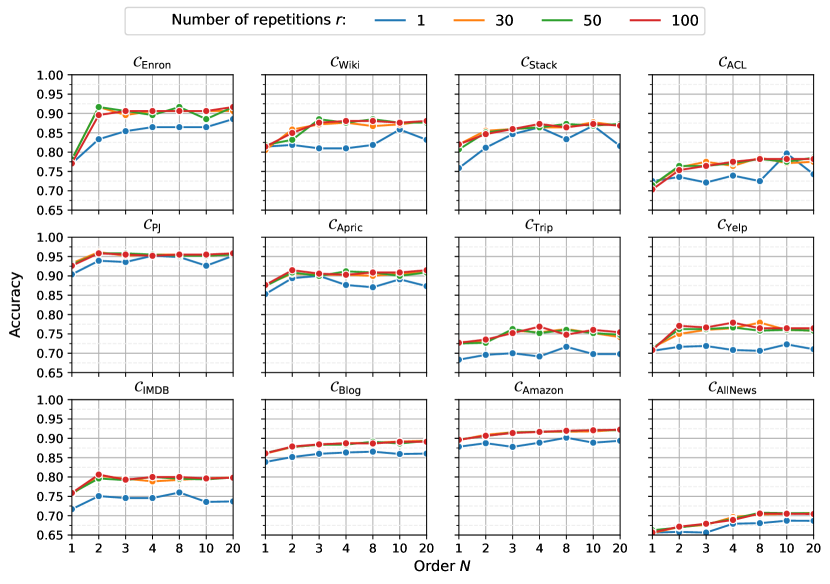
Figure 1: Accuracy results for different numbers of repetitions $r$ and orders of the $n$-gram model $N$ for each corpus.

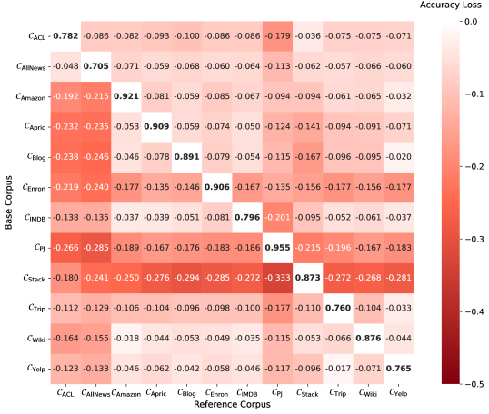
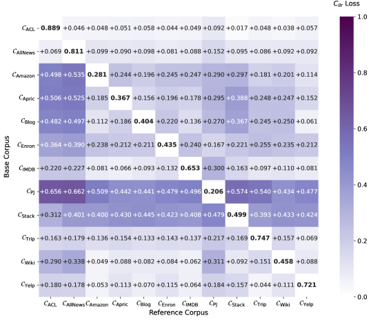
Figure 2: The loss in Accuracy (top) and $C_{\text{llr}}$ (bottom) results for cross-corpus comparison, i.e. evaluating on Base Corpus while using reference texts $\mathbb{D}_{\text{ref}}$ from Reference Corpus. Diagonal bold values denote the original Accuracy and $C_{\text{llr}}$, respectively. Darker shades denote a greater loss in performance.

Another important robustness test that we performed is the selection of the reference data. Reliance on external data is a potential limitation for any binary extrinsic AV methods, like IM. As explained in Section 1, IM, suffers a substantial loss in performance if the impostors are selected from another genre. LambdaG also has the crucial requirement that a reference corpus $\mathbb{D}_{\text{ref}}$ is collected and it is presumably important that $\mathbb{D}_{\text{ref}}$ is as compatible as possible, especially in genre but generally speaking in as many parameters as possible, with $\mathbb{D}_{\mathcal{A}}$ and $\mathbb{D}_{\mathcal{U}}$. To test the robustness of LambdaG to variations in $\mathbb{D}_{\text{ref}}$ type we ran 144 tests by pairing each of the twelve corpora to every other corpora. For example, we performed the analysis for $\mathcal{C}_{\mathrm{Enron}}$ but we used as $\mathbb{D}_{\text{ref}}$ $\mathcal{C}_{\mathrm{ACL}}$. We then calculated Accuracy and $C_{\text{llr}}$ for all combinations and we produced a plot for each metric displaying the resulting drop in performances when using a different $\mathbb{D}_{\text{ref}}$ (Figure 2).

Corpus	$C_{\text{llr}}\mbox{}(\lambda_{G})$	$C_{\text{llr}}\mbox{}(\Lambda_{G})$	$C_{\text{llr}}^{\text{min}}$
$\mathcal{C}_{\mathrm{Enron}}$	3.630	0.432	0.315
$\mathcal{C}_{\mathrm{Wiki}}$	2.026	0.457	0.405
$\mathcal{C}_{\mathrm{Stack}}$	5.716	0.499	0.411
$\mathcal{C}_{\mathrm{ACL}}$	18.038	0.885	0.636
$\mathcal{C}_{\mathrm{PJ}}$	2.000	0.254	0.143
$\mathcal{C}_{\mathrm{Apric}}$	2.811	0.397	0.337
$\mathcal{C}_{\mathrm{Trip}}$	2.666	0.752	0.715
$\mathcal{C}_{\mathrm{Yelp}}$	1.872	0.726	0.691
$\mathcal{C}_{\mathrm{IMDB}}$	2.714	0.648	0.626
$\mathcal{C}_{\mathrm{Blog}}$	2.969	0.424	0.403
$\mathcal{C}_{\mathrm{Amazon}}$	1.604	0.302	0.286
$\mathcal{C}_{\mathrm{AllNews}}$	9.920	0.812	0.797

Table 2: Values of $C_{\text{llr}}$ and $C_{\text{llr}}^{\text{min}}$ for $\lambda_{G}$ and for $\Lambda_{G}$ generated by calibrating $\lambda_{G}$ with the logistic regression calibration method. $C_{\text{llr}}^{\text{min}}$ is identical for both $\lambda_{G}$ and $\Lambda_{G}$.

The diagonal of Figure 2 (top) shows the same results reported in Table LABEL:tab:EvalResults, which function as the benchmark of performance for each row of the plot, corresponding to the corpus being tested. Overall the results suggest that LambdaG is extremely robust in many cases of genre variation, including some unrealistic genre combinations. This result is unexpected given how IM is instead very much dependent on the set of impostors [41]. For example, cross-corpus comparisons such as using $\mathcal{C}_{\mathrm{Yelp}}$ as reference for problems in $\mathcal{C}_{\mathrm{Amazon}}$ lead to very small losses in Accuracy and this is clearly explainable by the fact that both corpora contain reviews. However, certain results are more surprising, such as that using the academic papers from $\mathcal{C}_{\mathrm{ACL}}$ as reference data for problems in a corpus of chat logs such as $\mathcal{C}_{\mathrm{PJ}}$ leads to a performance loss of only 0.27 Accuracy, which is substantial but much less than expected given the disparity. This is a comparison that a human analyst would be unlikely to perform and therefore it is a real test of the lower limits in terms of robustness to reference corpora.

Looking at Figure 2 (top) row-wise, the most notable pattern is that the two corpora that suffer the most performance loss overall are $\mathcal{C}_{\mathrm{PJ}}$ and $\mathcal{C}_{\mathrm{Stack}}$. For $\mathcal{C}_{\mathrm{PJ}}$ the explanation is likely to be that it is the only corpus with sentences mostly corresponding to chat messages, and therefore any match of this corpus with other corpora results in at least this incompatibility. The chat logs in $\mathcal{C}_{\mathrm{PJ}}$ are also the texts with the lowest level of formality and highest degree of linguistic freedom among all corpora. For $\mathcal{C}_{\mathrm{Stack}}$ this result could be due to its hybrid genre character (forum posts on academic topics) or it could simply be due the use of several tags to mask mathematical expressions or computer code. When looking at Figure 2 column-wise, instead, the most notable pattern is that using $\mathcal{C}_{\mathrm{ACL}}$ or $\mathcal{C}_{\mathrm{AllNews}}$ as reference corpora tends to affect performance more drastically for the majority of corpora, which again could be explained by their relatively higher degree of formality compared to the other corpora. All in all this analysis suggests that, for $\mathcal{C}_{\mathrm{PJ}}$ and $\mathcal{C}_{\mathrm{Stack}}$ the reference corpus has a moderate impact on performance while for all other corpora it is only the use of $\mathcal{C}_{\mathrm{ACL}}$ or $\mathcal{C}_{\mathrm{AllNews}}$ as reference where this modest impact can be observed. For all other cross-corpus comparisons for most corpora the effect of the reference corpus is tolerable.

We also present the results for the $C_{\text{llr}}$ metric in Figure 2 (bottom). As explained in Section 5.4, a $C_{\text{llr}}$ value close to or equal to one means that the system is not providing any useful information for the case, while a $C_{\text{llr}}$ value higher than 1 means that results tend to be misleading (e.g. negative $\Lambda_{G}$ for a Y-problem). None of the cross-genre comparisons produce $C_{\text{llr}}$ higher than one, meaning that in all cases the values of $\Lambda_{G}$ are not misleading the analyst but can be, at worst, inconclusive with $\Lambda_{G}\approx 0$. These results support the principle that an analyst should always compile a reference data set that is as close as possible to the case data [52]. However, the results do also suggest that LambdaG is stable to small variations in genre.

The final test we carried out is a comparison of LambdaG as implemented in Algorithm 1 vs. LambdaG without applying the POSNoise function. The rationale for this test is to understand whether more authorial information can be extracted and exploited using this method beyond just grammatical structure. The results in Table 3 show that, regarding Accuracy and AUC, in all cases the proposed version of Algorithm 1 with the POSNoise pre-processing is better performing than a version of the algorithm without this pre-processing. The difference in Accuracy is not large but the method is clearly superior when the focus is entirely on grammar to the extent that adding information about meaning instead leads to adding noise in the authorial signal.

As explained in Section 5.3, the advantage of LambdaG is that it can be better interpreted than other methods. As a first step, the analyst can produce a ranking of all sentences in $\mathcal{D}_{\mathcal{U}}$ and then, additionally, each token can be color-coded according to its value of $\lambda_{G}$, similarly to COAV. Some of these visualizations explaining the features discovered are shown in Section 6.

	$\Delta$Acc.	$\Delta$AUC	$\Delta$F1	$\Delta$Prec.	$\Delta$Rec.	$\Delta$TP	$\Delta$FN	$\Delta$FP	$\Delta$TN
$\mathcal{C}_{\mathrm{Enron}}$	0.031	0.039	0.039	-0.017	0.083	4	-4	1	-1
$\mathcal{C}_{\mathrm{Wiki}}$	0.026	0.003	0.029	0.022	0.036	4	-4	-2	2
$\mathcal{C}_{\mathrm{Stack}}$	0.005	0.001	-0.002	0.047	-0.044	-5	5	-6	6
$\mathcal{C}_{\mathrm{ACL}}$	0.057	0.050	0.031	0.106	-0.050	-7	7	-23	23
$\mathcal{C}_{\mathrm{PJ}}$	0.009	0.005	0.010	0.001	0.019	3	-3	0	0
$\mathcal{C}_{\mathrm{Apric}}$	0.077	0.042	0.084	0.038	0.129	22	-22	-4	4
$\mathcal{C}_{\mathrm{Trip}}$	0.037	0.049	0.048	0.022	0.071	17	-17	-1	1
$\mathcal{C}_{\mathrm{Yelp}}$	0.057	0.046	0.063	0.043	0.083	20	-20	-7	7
$\mathcal{C}_{\mathrm{IMDB}}$	0.080	0.101	0.091	0.070	0.108	87	-87	-42	42
$\mathcal{C}_{\mathrm{Blog}}$	0.063	0.038	0.066	0.048	0.083	75	-75	-38	38
$\mathcal{C}_{\mathrm{Amazon}}$	0.046	0.030	0.046	0.041	0.050	60	-60	-49	49
$\mathcal{C}_{\mathrm{AllNews}}$	0.043	0.049	0.059	0.034	0.076	101	-101	-15	15
Table 3: Differences in evaluation results when applying the POSNoise function in LambdaG compared to omitting it. Positive values (shaded in blue) indicate results improvement, while negative values (shaded in red) indicate results degradation by using POSNoise.

4 Discussion

Our proposed LambdaG approach matches many desiderata of an AV method:

1. It works on both short and long documents;

2. It is not affected or minimally affected by topic or content;

3. It is stable to small genre variations in the reference corpus;

4. It is more interpretable by an analyst;

5. It is not computationally intensive and does not have a high run time;

6. Even though the algorithm is stochastic, it is effectively deterministic for $r\mathrel{\mathchoice{\raise 0.0pt\hbox{\scalebox{0.8}{\raise 0.0pt\hbox{$\displaystyle\gtrapprox$}}}}{\raise 0.0pt\hbox{\scalebox{0.8}{\raise 0.0pt\hbox{$\textstyle\gtrapprox$}}}}{\raise 0.0pt\hbox{\scalebox{0.8}{\raise 0.0pt\hbox{$\scriptstyle\gtrapprox$}}}}{\raise 0.0pt\hbox{\scalebox{0.8}{\raise 0.0pt\hbox{$\scriptscriptstyle\gtrapprox$}}}}}100$;

7. It has a theoretical foundation based on Cognitive Linguistic theories of language processing.

Section 3 showed evidence of the first six of these points as well as evidence that LambdaG outperforms other AV state-of-the-art methods. We believe that a possible reason to explain these results, especially considered the simplicity of the method compared to approaches such as SiamBERT, is precisely that LambdaG has a number of properties that make it consistent with knowledge about language processing gained from studies in Cognitive Science and Cognitive Linguistics.

Since the pioneering study of Mosteller and Wallace [79], it is well known that the frequency of functional items distinguish authors and this conclusion is also evident in the case of LambdaG. The reason why this is the case, however, has always been seen as a mystery in the field of authorship analysis and stylometry [56]. A connection between the unreasonable effectiveness of these functional items and Cognitive Linguistics has been proposed by Nini [82] and we believe that the success of LambdaG is additional evidence for these explanations.

Cognitive Linguistics models language as a complex adaptive system [9], where regularities emerge from the complexity of language used in interactions, like a phenomenon of the third kind [33]. This is partially evidenced by decades of linguistics studies on corpora which have revealed that the traditional conception of a grammar as an abstract set of phrase structure rules is untenable and that, instead, a better model of grammar is a lexicogrammar continuum that goes from fixed lexicalized expressions (e. g., “I don’t know”) to flexible templates (e. g., “the” X-er “the” Y-er) up to completely abstract structures (e. g., Doer Action Object).

This continuum roughly corresponds to the continuum between declarative memory, which is semantic/encyclopedic memory for facts and which tends to be conscious, and procedural memory, which is instead memory for the probabilistic prediction of patterns of sequences and that deals with subconscious knowledge of habits and skills [108]. The roles that these two memories play in language is clearly evidenced in cases of aphasia. When an impairment affects circuits of declarative memory, this gives rise to fluent aphasia, resulting in speech that is mostly constituted by function words like articles, prepositions, pronouns, and morphological forms but with lack of content words that contain meaning, leading to fluent but nonsensical speech comparable to POSNoise pre-processed data such as the one in Table 5. Instead, when the impairment is on procedural memory, then speech is only consisting of content words that are not connected through grammar [109]. These two memory systems work together and, typically, once a habit is formed through repetition then procedural memory takes over, leading to fluency of expression. This transition explains why languages tend to be heavily formulaic. For example, in English one can say big mistake but not large mistake, even though the formal grammar would seemingly have no problems with the latter expression, which is an adjective modifying a noun. What explains this reliance on formulaic expressions is the cognitive tendency to recur to memory as much as possible rather than creating something new every time we use language [108].

The way these units of procedural memory are formed is through the process of chunking: when two items that often go together are found together, then these two items can be treated as one, thus saving space in working memory [39, 21, 28]. In all effects, chunking is a process of information compression and, if the units of grammar are chunks, then the logical inference is that grammar itself can be thought of as a compressed version of a language or, equivalently, as a probability model. A probability model of only functional items is therefore quite like the Grammar Models used in this study.

Cognitive Linguistics also explains why each individual has a different and possibly unique grammar, a statement encapsulated by the Principle of Linguistic Individuality [82]. The status of unithood given by chunking is not discrete (e. g., something is or is not a unit) but a continuum of strength of unithood, where this strength is called entrenchment [32, 97]. Because entrenchment is dependent on exposure and usage, it is fundamentally personal and idiosyncratic. It is for this reason that Langacker hypothesized that “the set of units mastered by all members of a speech community might be a rather small proportion of the units constituting the linguistic ability of any given speaker” [71], a hypothesis that is finding increasing empirical support [82]. For example, for most if not all speakers of English the entrenchment for a sequence such as “of the” is maximal, meaning that they can produce it effortlessly and unconsciously as a single unit. In contrast, a sequence such as “the of” would not be a unit for speakers of English because it is virtually never encountered or used. If a speaker of English encounters this sequence, they would decompose it as a structure made up of two units, “the” and “of”. In between these two extreme examples there is a lot of freedom as to what counts as a unit for a person or another, depending on what each individual has automatized in their procedural memory. For example, an individual $\mathcal{A}_{1}$ might have a very entrenched sequence such as “it is known that” when writing academic articles while an individual $\mathcal{A}_{2}$ might have “it is well established that”. These sequences will then have open slots ready to be filled in with the appropriate meaning. This kind of phenomenon theorized by Langacker can be seen at play in this method, especially when looking at the examples of idiosyncratic structures in Section 6. As briefly mentioned in Section 5.3, therefore, the likelihood of a token given a context assigned by an author $\mathcal{A}$’s Grammar Model, $P(t|c;G_{\mathcal{A}})$, can be seen as a way to measure the level of entrenchment of token $t$ in context $c$ for $\mathcal{A}$ . The higher the entrenchment, the more likely it is that $\mathcal{A}$ is using procedural memory and that it is therefore performing an unconscious routine that constitutes a unit for this individual.

There have been other attempts at modeling the grammar of an author in the past for AV or AA purposes [24, 7, 37] but these methods relied too much on Part of Speech tags or on syntactic trees which are often not compatible with predictions made in Cognitive Science and Cognitive Linguistics. As explained above, the picture of grammar painted by Cognitive Linguistics is much more lexically-based and word-idiosyncratic. For example, the preposition “of” in English behaves very oddly compared to other prepositions [100]. Giving it the same Part of Speech label as to other prepositions is therefore going to obscure a lot of important grammatical information. Instead, a topic-masking method such as POSNoise is much more consistent with the predictions of Cognitive Linguistics because it leaves the function items unaffected while only obscuring those items are more likely to change from context to context depending on the communicative needs.

To sum up, the model of an individual’s grammar that emerges from Cognitive Science and Cognitive Linguistics is one that is very much compatible with the Grammar Models used for LambdaG. Although language modeling is seen in computational linguistics as a tool and not necessarily a realistic representation of language, evidence from Cognitive Linguistics suggests that, in reality, a language model, while not being realistic as a model of linguistic production, is instead a plausible representation of how knowledge of grammar is stored in the mind. The mechanisms of such a sequential processing can be efficiently represented through the short-term correlations captured by $n$-gram models as done in this work.

A deeper connection between LambdaG and approaches to AV based on language modeling or, as for COAV, on compression algorithms can also be drawn, thus offering a plausible explanation for their success. Through the lenses of Information Theory, the average $P(s;G)$ for each $s\in\mathcal{D}$ can be also seen as an estimate of the cross-entropy rate of the Grammar Model $G$ against the probability distribution of grammatical tokens that generates $\mathcal{D}$. In language modeling literature, the cross-entropy is often exponentiated to calculate the perplexity of a document given a model. Because for LambdaG the two alternative Grammar Models are compared in relation to the same $\mathcal{D}$, for the purposes of this AV application, $\lambda_{G}$ is equivalent to comparing the perplexities of the candidate author’s model vs. the reference model given the same $\mathcal{D}$ and assign the document to the candidate author if this perplexity is lower. The cross-entropy rate can also be interpreted as the average length in bits of a binary encoding of grammatical tokens for a data-compression scheme that is optimized for the probability distribution $P(\cdot;G)$. For this reason, a language model can be seen as a text-compression scheme. This connection thus links compression and language model AV methods like LambdaG and COAV to the Cognitive Linguistics conception of an individual’s grammar as a compressed representation of real language usage encountered by said individual.

In addition to the successful results of LambdaG, we note that the qualitative explorations reported in Section 6 also constitute evidence that LambdaG captures linguistic behavior compatible with these Cognitive Linguistic explanations. Although it is impossible to know for certain the effective mental status of the sequences found in the examples in Section 6, we propose that it is plausible to believe that the authors of these texts do not know that they use the sequences of tokens highlighted in red or that these sequences identify them in the general population. These sequences, which are often seemingly unremarkable (e. g., “enough to be ADVERB VERB” or “so PRONOUN cant”), can be extremely idiosyncratic and uniquely used only by the candidate author. Given the fact that the problems analyzed in this paper involve relatively short texts (the longest texts are just around 2000 tokens), we must conclude that these idiosyncratic units are easy to find and this conclusion therefore strongly supports Langacker’s proposal that most units in a language are not shared by many individuals.

We believe that additional evidence towards this assertion is given by the results of the cross-reference experiments. Controlling for genre compatibility is probably the hardest problem in AV and AA. LambdaG is very robust to this variation in many cases, much more than expected given the results of similar tests carried out on IM [41]. This is despite the incredible challenges in some of the comparisons, such as in the analysis of the $\mathcal{C}_{\mathrm{PJ}}$ chat logs using as reference the academic papers in $\mathcal{C}_{\mathrm{ACL}}$. The genre differences between these two corpora cannot be greater and therefore it is hard to believe that the method is not performing at chance level. A possible explanation for the success of LambdaG in these circumstances is that the reference corpus effectively does not play a major role. If individual grammars are so different from each other, then the role of the reference corpus could be to just weight down the those units that are well-entrenched for most individuals (e. g., of the) and that therefore carry almost no authorial information. If this explanation is correct, then this means that once these common units are taken into account, the rest is idiosyncratic enough to be identifying.

Finally, due to the fact that these idiosyncratic units are easy to find within as little as 1,000 to 2,000 tokens, we add that a consequences of the present findings and of the underlying Cognitive Linguistic theory is that the grammar of a person can be seen as a behavioral biometric [82]. Similarly to handwriting, gait, typing patterns, computer mouse usage, and most features of human voice, grammar is also a cognitive process relying on procedural memory that strengthens with habit and repetition. We propose that this is the explanation underlying most if not all AV and AA methods that, by measuring the frequency of functional items, are indirectly analyzing the idiosyncratic grammar of an individual. LambdaG tends to be more successful probably because it is measuring the same phenomenon more directly.

4.1 Limitations and future research

We argue that future research should therefore continue in this direction of extracting better representations of the grammar of an individual. The POSNoise algorithm used here is language dependent and suffers from the use of general part of speech categories that are not compatible with Cognitive Linguistics, which instead predicts the existence of categories that are more semantic in nature and at lower degrees of abstractness. New future methods should embrace the close relationship between Cognitive Linguistics and Information Theory to gain more insight into grammar, which could consequently lead to further breakthroughs in AV.

In addition, LambdaG is still affected by genre differences and performs less well in registers where there is less variation, such as academic prose. These two last limitations affect more or less all existing algorithms which are outperformed by LambdaG, which could mean that these limitations are intrinsic to AV and, indeed, there would be good linguistic reasons for why this would be the case. Despite these limitations, future methods based on a better understanding of grammar could still lead to more progress. In this respect, the reliance on a reference corpus could also be seen as a limitation of any binary AV method. The tendency for future AV methods should be to increase the power of unary methods that only need a test dataset.

Finally, another limitation of the present paper is that the research was carried out entirely on English. The theory underlying LambdaG generalizes to other languages and for this reason the prediction is that it would also outperform the same baseline methods in other languages. The way Grammar Models are trained in languages with a rich morphology is likely to be different, however. Different tokenizers might have to be employed as well as different algorithms such as POSNoise to focus the model on the grammatical aspects of the text. Another goal for the future would therefore be to find a language-independent variant of LambdaG.

4.2 Final Remarks

The advances in AV made in this paper were possible because of the collaboration between Linguistics and Natural Language Processing. In the 2022 edition of the PAN competition on AV, Stamatatos et al. [104] concluded that “all submissions, despite their increased level of sophistication in most of the cases, were outperformed by a naive baseline based on character $n$-grams and cosine similarity” thus noticing a situation of stall in the progress on AV. Knowledge from Linguistics could resolve these stalls, as demonstrated in this paper, by shifting the point of view rather than adding more computational sophistication or making algorithms more complex. The method and philosophy introduced in the present work offer significant advancements in integrating Linguistics theory and Computer Science methods towards a new paradigm in AA and AV where these two fields are better harmonized. The task of identifying a writer from the language used in a text is really an application of Linguistics and there are various reasons for computational methods to maintain a close relationship with Linguistics. Firstly, these methods directly or indirectly exploit linguistic patterns that require knowledge of Linguistics to be described and understood. Secondly, knowledge of Linguistics is needed to understand and potentially explain in a court of law the reasons why these patterns identify or exclude a certain author. We believe that the work in this paper has made some significant advances in AV while also proposing and stimulating a paradigm change to move on from the impasse described by Stamatatos [104] towards new AV methods that are not only well-performing but also scientifically meaningful.

5 Methods

In this section, we present the more technical details of our work, first with an introduction to the corpora we have compiled to evaluate LambdaG, then by providing more details about the POSNoise content-masking algorithm as well as the details of the Kneser-Ney smoothing algorithm, the likelihood ratio framework for forensic sciences and, finally, the Siamese neural network baseline method, SiamBERT, developed for this analysis.

5.1 Corpora

To evaluate LambdaG, we compiled a collection of 12 corpora covering a variety of challenges. These include, for instance, very short texts ($\approx 5$ sentences), texts with a lack of coherence, texts with excessive use of slang, texts (of the same author) written at different times, texts with opposing topics, texts with distorted writing style caused by post-editing, texts with truncated sentences as well as non-standard spellings and missing spaces. In total, the corpora comprise 17,306 verification cases, were each corpus $\mathcal{C}=\{c_{1},c_{2},\ldots\}$ is split into author-disjunct training and test partitions based on a 40/60 ratio, resulting in 6,402 training and 10,904 test verification cases. Each $c\in\mathcal{C}$ denotes a verification case $(\mathcal{D}_{\mathcal{U}},\mathbb{D}_{\mathcal{A}})$, where $\mathcal{D}_{\mathcal{U}}$ is an unknown document and $\mathbb{D}_{\mathcal{A}}$ is a set of example documents of the known author $\mathcal{A}$. To counteract population homogeneity, a known bias in authorship verification described by Bevendorff [11], we ensured that for each author $\mathcal{A}$ there are exactly two (one same-authorship (Y) and one different-authorship (N)) verification cases. Furthermore, we constructed all corpora so that the number of Y- and N-cases is equal, in other words, all training and test corpora are (strictly) balanced. In what follows, we describe all corpora in detail, underline their respective challenges and explain the pre-processing steps we have performed. A compact overview of the 12 corpora, including their partitioning into training and test corpora, as well as further information can be found in Table 4.

Corpus	Genre	Topic	Partition	$|\mathcal{C}|$	avg$(\mathbb{D}_{\mathcal{A}})$	avg$(\mathcal{D}_{\mathcal{U}})$
$\mathcal{C}_{\mathrm{Enron}}$	E-mails	Related	$\mathcal{C_{\,\textrm{train}}}$	64	783 (3866)	906 (4432)
			$\mathcal{C_{\,\textrm{test}}}$	96	763 (3808)	882 (4391)
$\mathcal{C}_{\mathrm{Wiki}}$	Wikipedia talk pages	Related	$\mathcal{C_{\,\textrm{train}}}$	150	467 (1266)	614 (1654)
			$\mathcal{C_{\,\textrm{test}}}$	226	492 (1328)	626 (1699)
$\mathcal{C}_{\mathrm{Stack}}$	Q & A posts	Cross	$\mathcal{C_{\,\textrm{train}}}$	150	2204 (11247)	1972 (9956)
			$\mathcal{C_{\,\textrm{test}}}$	228	2306 (11803)	2114 (10700)
$\mathcal{C}_{\mathrm{ACL}}$	Scientific papers	Related	$\mathcal{C_{\,\textrm{train}}}$	186	1707 (9497)	2553 (14196)
			$\mathcal{C_{\,\textrm{test}}}$	280	1479 (8250)	2492 (13913)
$\mathcal{C}_{\mathrm{PJ}}$	Chat logs	Related	$\mathcal{C_{\,\textrm{train}}}$	208	594 (2329)	752 (2946)
			$\mathcal{C_{\,\textrm{test}}}$	312	592 (2324)	754 (2967)
$\mathcal{C}_{\mathrm{Apric}}$	Forum posts	Related	$\mathcal{C_{\,\textrm{train}}}$	228	796 (3900)	825 (4023)
			$\mathcal{C_{\,\textrm{test}}}$	340	799 (3921)	817 (4020)
$\mathcal{C}_{\mathrm{Trip}}$	Travel reviews	Related	$\mathcal{C_{\,\textrm{train}}}$	120	658 (3169)	249 (1186)
			$\mathcal{C_{\,\textrm{test}}}$	480	698 (3344)	252 (1202)
$\mathcal{C}_{\mathrm{Yelp}}$	Hotel/restaurant reviews	Related	$\mathcal{C_{\,\textrm{train}}}$	320	139 (637)	167 (767)
			$\mathcal{C_{\,\textrm{test}}}$	480	139 (640)	167 (768)
$\mathcal{C}_{\mathrm{IMDB}}$	Movie reviews	Mixed	$\mathcal{C_{\,\textrm{train}}}$	400	658 (3151)	374 (1796)
			$\mathcal{C_{\,\textrm{test}}}$	1600	690 (3291)	366 (1753)
$\mathcal{C}_{\mathrm{Blog}}$	Blogs posts	Mixed	$\mathcal{C_{\,\textrm{train}}}$	1200	742 (3416)	881 (4086)
			$\mathcal{C_{\,\textrm{test}}}$	1800	740 (3385)	882 (4061)
$\mathcal{C}_{\mathrm{Amazon}}$	Product reviews	Mixed	$\mathcal{C_{\,\textrm{train}}}$	1600	861 (4010)	869 (4041)
			$\mathcal{C_{\,\textrm{test}}}$	2400	860 (4009)	868 (4041)
$\mathcal{C}_{\mathrm{AllNews}}$	News articles	Mixed	$\mathcal{C_{\,\textrm{train}}}$	1776	675 (3629)	941 (5064)
			$\mathcal{C_{\,\textrm{test}}}$	2662	680 (3665)	942 (5071)

Table 4: All used corpora and their key statistics. Notation: $|\mathcal{C}|$ denotes the number of verification cases in each corpus $\mathcal{C}$, while avg$(\mathbb{D}_{\mathcal{A}})$ and avg$(\mathcal{D}_{\mathcal{U}})$ denotes the average token count (and character count in parentheses) of all $\mathcal{D}_{\mathcal{A}}\in\mathbb{D}_{\mathcal{A}}$ and $\mathcal{D}_{\mathcal{U}}$, respectively.

5.1.1 $\mathcal{C}_{\mathrm{Enron}}$

The $\mathcal{C}_{\mathrm{Enron}}$ corpus was derived from the well-known Enron Email Dataset, which has been used in many AV and AA studies, including [17, 18, 19, 27, 31, 72, 83, 112, 4], as well as in many other research areas. The Enron email dataset has gained considerable popularity in the authorship analysis community, likely due to the fact that it is (to the best of our knowledge) the only publicly available corpus of real-world emails with a guaranteed ground truth. Similar to previous AV studies, we also reduced the initial set to a smaller number of authors (in our case from 150 to 80), as only a few suitable emails were available for some of the authors. In total, $\mathcal{C}_{\mathrm{Enron}}$ consists of 362 documents, with each document representing a concatenation of several emails from the corresponding author in order to obtain a sufficient length. Since the emails in the Enron Email Dataset contain a wide range of noise, extensive preprocessing was necessary. To this end, we decided to manually preprocess all considered texts and instead create individual replacement rules for various types of noise. First, we removed URLs, email headers, greeting/closing formulas, email signatures, (phone) numbers, quotes as well as various non-letter repetitions. Next, we normalized UTF-8 symbols and, in a final step, replaced multiple consecutive spaces, line breaks and tabs with a single space. A similar preprocessing procedure was also described by Brocardo et al. [17, 18].

5.1.2 $\mathcal{C}_{\mathrm{Wiki}}$

The $\mathcal{C}_{\mathrm{Wiki}}$ corpus consists of 752 excerpts from 288 Wikipedia talk page editors taken from the Wikipedia sockpuppets dataset, which was released by Solorio et al. [101]. The original dataset contains two partitions comprising sockpuppets and non-sockpuppets cases, where for $\mathcal{C}_{\mathrm{Wiki}}$ we only considered the latter subset. In addition, we did not use the full range of authors within the non-sockpuppets cases, as there were not sufficiently long texts available for each of the authors. Regarding the selected texts, we removed Wiki markup, timestamps, URLs and other types of noise. Furthermore, we removed sentences containing many numbers, proper names and near-duplicate string fragments as well as truncated sentences.

5.1.3 $\mathcal{C}_{\mathrm{Stack}}$

The $\mathcal{C}_{\mathrm{Stack}}$ corpus consists of 567 posts from 189 users crawled from the question-and-answer (Q & A) network Stack Exchange in 2019. The network comprises 173 Q & A communities, with each community focusing on a specific topic (e. g., linguistics, computer science, philosophy, etc.). For the compilation of $\mathcal{C}_{\mathrm{Stack}}$, which represents a cross-topic corpus, we collected questions and answers from users who were simultaneously active in the two thematically different communities Cross Validated ($\mathcal{S}_{1}$) and Academia ($\mathcal{S}_{2}$). The verification cases were constructed as follows. Each verification case consists of exactly two documents, a known and an unknown document $\mathcal{D}_{\mathcal{A}}$ and $\mathcal{D}_{\mathcal{U}}$. Within the Y-cases, $\mathcal{D}_{\mathcal{A}}$ and $\mathcal{D}_{\mathcal{U}}$ were taken from $\mathcal{S}_{1}$ and $\mathcal{S}_{2}$ respectively, while within the N-cases $\mathcal{D}_{\mathcal{A}}$ and $\mathcal{D}_{\mathcal{U}}$ were taken from the same community $\mathcal{S}_{1}$. Due to the cross-topic nature of this corpus, AV methods that utilize topic-based features are more likely to provide inverse predictions (i. e., N-cases are more likely to be classified as Y and vice versa) while AV methods that use topic-agnostic features behave more robustly. Another challenge of $\mathcal{C}_{\mathrm{Stack}}$ is that the corpus is very unbalanced with respect to the length of the documents, with lengths between 3014 and 20476 characters. To avoid stylistic distortions from the outset, we only used the original posts of the respective authors for all texts in $\mathcal{C}_{\mathrm{Stack}}$, while subsequent edits by third parties (for the purpose of spelling or stylistic improvement) were excluded. In addition, we replaced equations/formulas, numerical values (e. g., percentages and currency values), dates, references and URLs with appropriate placeholders. The reason why we did not omit the affected sentences and instead opted for this approach was that we wanted to keep as much text content per author as possible to ensure a sufficient number of authors.

5.1.4 $\mathcal{C}_{\mathrm{ACL}}$

The $\mathcal{C}_{\mathrm{ACL}}$ corpus comprises 466 excerpts from scientific papers by a total of 233 researchers, taken from the computational linguistics archive ACL Anthology. The corpus was constructed in such a way that there are exactly two papers for each author, dating from different time periods. The average time span between the two documents of each author is approximately 15.6 years, while the minimum and maximum time spans are 8 and 31 years, respectively. In addition to the temporal aspect of the documents in $\mathcal{C}_{\mathrm{ACL}}$, another challenge of this corpus is the formal language, in which the use of stylistic devices (e. g., repetitions, metaphors or rhetorical questions) is more restricted in contrast to other text types such as chat logs, forum posts or product reviews. For the original papers, we have tried to limit the content of each text as much as possible to those sections that consist mainly of natural language text (e. g., abstract, introduction, discussion, conclusion or future work). To ensure that the extracted fragments are consistent with the remarks of Bevendorff et al. [11], we decided to preprocess each paper excerpt in $\mathcal{C}_{\mathrm{ACL}}$ (semi-)manually. Among other things, we removed tables, quotations and sentences that contained a large amount of non-linguistic content such as mathematical constructs as well as specific names of researchers, systems and algorithms. We also replaced (inline) mathematical expressions, references (e. g., “[12]”, “[SHL13]”), endophoric markers, numeric values and URLs with appropriate placeholders, as we did with the texts in $\mathcal{C}_{\mathrm{Stack}}$.

5.1.5 $\mathcal{C}_{\mathrm{PJ}}$

The $\mathcal{C}_{\mathrm{PJ}}$ corpus comprises a total of 738 chat logs from 260 sex offenders collected from the Perverted-Justice portal. The chat logs were obtained from older instant messaging clients (e. g., MSN, AOL and Yahoo), whereby for each conversation we ensured that only the offender’s chat lines were extracted based on the annotations provided by the portal. To maximize variability in terms of conversation content, we selected chat lines from different messaging clients as well as from different time spans (where possible). A major challenge of $\mathcal{C}_{\mathrm{PJ}}$ is that it contains texts characterized by excessive use of non-standard English and also contains many chat-specific abbreviations and other forms of noise. This in turn makes it difficult to extract syntax-based features such as POS tags from the texts, at least when using NLP models trained on texts written in standard English (e. g., news articles or scientific documents). Another challenge of $\mathcal{C}_{\mathrm{PJ}}$ is that the text fragments it contains are very short, which in turn limits stylistic variability. In contrast to $\mathcal{C}_{\mathrm{Enron}}$, we have automatically pre-processed the texts in this corpus. Among other things, we sorted out chat lines with less than 5 tokens and 10 characters or those containing usernames, timestamps, URLs and words with many repeating characters (e. g., “mmmhhhmm”, “heeheehee” and “:-*:-*:-*:-*:-*:-*:-*:-*”). To further increase the variability in the content of each chat log $X$, we made sure that all contained lines $(x_{1},x_{2},\ldots,x_{m})$ are different from each other. For this purpose, we applied a string similarity function to each pair $(x_{i},x_{j})$ with $i\neq j$. As a metric for string similarity, we chose the Levenshtein distance based on a threshold of 0.25, which we considered appropriate for our purposes. All pairs of lines that exceeded this threshold were discarded with respect to the text fragments.

5.1.6 $\mathcal{C}_{\mathrm{Apric}}$

The $\mathcal{C}_{\mathrm{Apric}}$ corpus comprises 1,395 forum posts from 284 users crawled from the portal The Apricity - A European Cultural Community. To compile the $\mathcal{C}_{\mathrm{Apric}}$, we ensured that all posts within each verification case were collected from different sub-forums covering a variety of topics, including anthropology, genetics, race and society and ethno-cultural discussion. We then pre-processed each post and removed certain markup tags, URLs, forum signatures, quotations (as well as nested quotations that contained the original author’s content), and other types of noise, similar to what we did with the texts within the $\mathcal{C}_{\mathrm{Enron}}$ corpus. However, despite the pre-processing, some textual peculiarities remained in the texts, such as truncated sentences, spelling errors and missing spaces between adjacent words or between a punctuation mark and the following word. These can be seen as a challenge of $\mathcal{C}_{\mathrm{Apric}}$, especially with regard to AV methods that use features based on word lists.

5.1.7 $\mathcal{C}_{\mathrm{Trip}}$

The $\mathcal{C}_{\mathrm{Trip}}$ corpus comprises reviews from 300 bloggers extracted from the Webis TripAdvisor Corpus 2014 published by Trenkmann and Spiel [107]. As the original corpus was not intended for the purposes of AV, we reformatted the data accordingly. While inspecting the data, we found that most of the included reviews were already of reasonable quality, so we only carried out moderate pre-processing. Among other things, we adjusted spaces next to punctuation marks (e. g., “( alight” $\rightarrow$ “(alight”)) and normalized many character repetitions to a maximum of three characters (e. g., “(!!!!!” $\rightarrow$ “!!!”). Besides, we excluded reviews that contained too many named entities and we discarded authors for which only one review was available.

5.1.8 $\mathcal{C}_{\mathrm{Yelp}}$

The $\mathcal{C}_{\mathrm{Yelp}}$ corpus comprises 2,400 reviews written by 400 so-called “Yelplers” extracted from the well-known Yelp dataset. The corpus was developed with several challenges in mind. First, compared to all other corpora we have compiled, it contains the shortest texts, with each $\mathcal{D}_{\mathcal{U}}$ consisting of at most ten sentences. For this reason, the stylistic variability within these texts is correspondingly limited. Secondly, many reviews were written at different times (in several cases often about four years apart), so linguistic changes are to be expected in reviews written by the same person. Thirdly, most of the texts in the $\mathcal{C}_{\mathrm{Yelp}}$ are restaurant reviews, which focus heavily on similar topics such as food, atmosphere and taste experiences. To a lesser extent, however, other forms of reviews are also included in the corpus (e. g., about wedding or clothing stores), which are accompanied by linguistic and also stylistic diversity with respect to the authors. Fourth, some of the reviews contain a mixture of moderate and colloquial writing styles. Regarding the latter, we observed certain spelling variations in the texts (e.g. missing apostrophes within contractions), which may result in noticeable loss of features for AV methods that rely on word lists. For the review texts in $\mathcal{C}_{\mathrm{Yelp}}$, we performed the following pre-processing steps. Sentences containing capitalized words throughout were removed (e. g., “I WAITED 4 HOURS IN THE BEND AND COULDN’T GET IN!!!!!!!!”), as were sentences containing quotes and many repetitive characters (e. g., “wait for a heart attack!!!!! Incompetent staff!!!! will never come here again!!!!”). Moreover, we removed sentences that only consist of single words (e. g., “fraud. Fraud. Lies.”) as well as review-type summaries such as “Quality: 10/10; Service: 9/10; Ambience/Location: 10/10; Overall: 9.5/10”.

5.1.9 $\mathcal{C}_{\mathrm{IMDB}}$

The $\mathcal{C}_{\mathrm{IMDB}}$ corpus consists of reviews from a total of 1000 IMDB users taken from the IMDB-1M Dataset published by Seroussi et al. [99]. From the original dataset, only the review texts and corresponding author names (more precisely, user IDs) were selected, while other metadata were discarded. Analogous to $\mathcal{C}_{\mathrm{Trip}}$, here we also performed a slight preprocessing since the quality of the texts was already suitable for the AV task. Among others, we normalized spaces adjacent to punctuation marks (e. g., “but . . . I” $\rightarrow$ “but... I”) and replaced year numbers with a placeholder (e. g., “1982” $\rightarrow$ “YEAR”). Furthermore, we also excluded authors for whom only one review was available as we did for $\mathcal{C}_{\mathrm{Trip}}$.

5.1.10 $\mathcal{C}_{\mathrm{Blog}}$

The $\mathcal{C}_{\mathrm{Blog}}$ corpus comprises 6,000 documents written by 1,500 bloggers, taken from the well-known Blog Authorship Corpus released by Schler et al. [96]. The original dataset comprises 681,288 posts of 19,320 bloggers and was collected from blogger.com in 2004. However, a large proportion of the posts were not suitable for our purposes for various reasons. For example, many posts consisted of non-English content or contained too much noise (e. g., superfluous strings, duplicate phrases, quotes, etc.) that was difficult to preprocess without losing too much text for the respective authors. In addition, the amount of text was insufficient in itself for many authors. Therefore, we only considered a smaller fraction of the original corpus. To counteract various noise types, we first sampled sentences from the original posts and ensured that each sentence is solely restricted to (case-sensitive) English letters, spaces and standard punctuation marks. From the resulting texts we then removed sentences containing repeated characters (e. g., “?!??!”, “---” and “-.-;;”) and words (e. g., “FUN!! FUN!! FUN!!” and “kekeke”), as well as sentences with many capitalized words (e. g., “i am saying that WHOEVER HAS OPTUS PLEASE TELL ME”). Besides, we discarded sentences containing URLs, gibberish strings (e. g., “rak;db’dfth6yortyi95”, “aDr0” and “w00t”) as well as truncated sentences. Finally, we concatenated the preprocessed sentences into a single document, which in turn led to a disruption of the coherence of the resulting texts. Similar to $\mathcal{C}_{\mathrm{PJ}}$, the texts in $\mathcal{C}_{\mathrm{Blog}}$ also exhibit an excessive amount of non-standard English expressions such as “w8 4” (wait for), “b4” (before), “2day” (today), “sum1’s” (someone’s) and “jnr” (junior). This can be seen as another challenge of $\mathcal{C}_{\mathrm{Blog}}$, since the spelling of such words is not always consistently adhered to with respect to the authors.

5.1.11 $\mathcal{C}_{\mathrm{Amazon}}$

The $\mathcal{C}_{\mathrm{Amazon}}$ corpus consists of 10,000 reviews written by 2,000 users, which were taken from the Amazon Product Data corpus published by McAuley et al. [74]. The original dataset contains approximately 143 million product reviews of the online marketplace Amazon collected between 1996 and 2014. While this dataset possesses a comprehensive structure that includes reviews (ratings, text, helpfulness votes), product metadata (descriptions, category information, price, brand, and image features) and links (also viewed/bought graphs), we only used the reviewer IDs, their corresponding texts as well as the category information to compile our $\mathcal{C}_{\mathrm{Amazon}}$ corpus. Based on the latter, we selected for each author review texts from distinct product categories (in total there are 17 categories including electronics, movies and TV and office products), so that (analogous to the $\mathcal{C}_{\mathrm{Reddit}}$ corpus) $\mathcal{C}_{\mathrm{Amazon}}$ represents a mixed-topic corpus. Regarding the texts that came from the Amazon Product Data corpus, we performed several preprocessing steps before selecting them for $\mathcal{C}_{\mathrm{Amazon}}$. Among others, we normalized HTML-encoded punctuation marks with respect to their mapped characters (for example, " $\rightarrow$ " or ’ $\rightarrow$ ’). In addition, we have added spaces between punctuation marks and adjacent words (e. g., “‘‘daily use.I also’’” $\rightarrow$ “daily use I also”) to allow for better separation of sentences. Furthermore, we removed sentences containing various forms of noise such as words with repetitive characters (e. g., “****update*****” or “mix.....it”), many capitalized words “VERY NICELY MADE AND THE COLOR IS BEAUTIFUL”, non-natural strings (e. g., “A++++”, “(48x18x21)” or “(27 & 23 Lbs)”) as well as quotes.

5.1.12 $\mathcal{C}_{\mathrm{AllNews}}$

The $\mathcal{C}_{\mathrm{AllNews}}$ corpus consists of 4,438 news articles written by 2,219 authors. The articles stem from the large well-known All the News 2.0 dataset, which consists of 2.7 million news articles and essays from 27 American news agencies and podcasting companies. From these, we limit ourselves to a single source, namely Reuters, which contains the largest number of news articles (840,094 in total). However, since not all articles were suitable for the creation of $\mathcal{C}_{\mathrm{AllNews}}$, it was necessary to preprocess the initial Reuters subset accordingly. First, we discarded all authors who wrote only a single article, as otherwise there is no suitable possibility to construct two verification cases for each author. Next, we sorted all articles of each author by their publication year and kept only four articles (the two oldest and the two newest). The main reasons for this were firstly to maximize the stylistic variation of each author and secondly to ensure sufficient length of the resulting documents, which in some cases were massively shortened by the pre-processing. Based on the four documents per author, the pre-processing was performed as follows. First, we removed all quotations (which are very common due to the nature of news articles) to mitigate the degree of stylistic distortion. Next, we removed headlines, sentences that consisted of more than 40 percent named entities and/or numeric tokens (e. g., dates, amounts of money, percentages, etc.), and article signatures that contained names of people who reported, wrote, and edited the articles. Finally, we normalized apostrophes (e. g., “’” $\rightarrow$ “’”) and replaced multiple consecutive spaces with a single space. The pre-processing procedure severely impaired the coherence of the resulting documents, as the natural order of many sentences was no longer given and some sentences also resulted in a truncated form. The impaired coherence can be seen as a challenge of this corpus, as AV methods that use implicit features (e. g., character/word $n$-grams) may capture “artificial features” that occur across sentence boundaries. Another challenge of $\mathcal{C}_{\mathrm{AllNews}}$ is that the documents often have been edited by other authors (e. g., the editor-in-chief) before online publication, so the original writing style of the articles may be distorted to some extent. Unlike the Stack Exchange network, All the News 2.0 does not provide metadata indicating which specific parts of the original article have been edited. Therefore, it was not possible for us to remove these afterwards.

5.2 Topic-Masking via POSNoise

Authorship verification constitutes a similarity detection problem in which the subject of the similarity determination is the language of the author rather than other document aspects such as the topic [42]. However, a large proportion of existing AV methods including [1, 17, 19, 22, 69, 70, 72, 80, 88] use features that are directly influenced by the topic and thus run the risk of biasing their predictions accordingly. To counteract the problem of biased predictions regarding LambdaG, which also employs topic-affected features, we apply topic masking to all documents in our corpora. Topic masking is an approach to pre-process texts in such a way that topic-dependent text units (e. g., words, phrases, etc.) are masked by appropriate placeholders, while grammatical text units (e. g., determiners, conjunctions, contractions, prepositions, pronouns, auxiliary verbs, quantifiers, transitional phrases, etc.) are retained within the texts. Of the few topic masking approaches published in the literature, we chose POSNoise presented by Halvani and Graner [42], which proved to outperform the previously published topic masking approach called TextDistortion [103] in 34 out of 42 cases, with an increase in accuracy of up to 10%.

Corpus	Original / topic-masked sentences
$\mathcal{C}_{\mathrm{Wiki}}$	If they actually censor anything is another question.
	If they © Ø anything is another #.
$\mathcal{C}_{\mathrm{Stack}}$	When I took the course, I ended up not being able to learn from the professor
	When I took the #, I Ø up not being @ to Ø from the #
$\mathcal{C}_{\mathrm{PJ}}$	going to wash clothes ,call me,tim
	going to Ø # ,call me,§
$\mathcal{C}_{\mathrm{Yelp}}$	Our meal started with a basket of freshly baked baguette and focaccia.
	Our # started with a # of © Ø # and #.
$\mathcal{C}_{\mathrm{Blog}}$	Then, Anna, Peter and I all went to baker’s Square.
	Then, §, § and I all went to #’s §.
$\mathcal{C}_{\mathrm{Amazon}}$	I got a new mascara that was impervious to makeup remover
	I got a @ # that was @ to # #

Table 5: Comparison between the original texts and their resulting topic-masked representations generated by POSNoise [42, Algorithm: 1]. The semantics of the placeholders can be looked up in [42, Table: 2].

5.3 N-Gram Language Modelling with Kneser-Ney Smoothing

This section provides a self-contained introduction to (modified) Kneser-Ney smoothing [62, 25]. Our main purpose is to provide the reader with all necessary details required to reproduce our AV method. For a more in-depth discussion of probabilistic and language modeling aspects, as well as for comparisons with other smoothing algorithms, we refer the reader to the original references [62, 26].

5.3.1 Basic Definitions and Notation

We assume we are given a dictionary $\mathcal{T}\mbox{}$ and a corpus $\mathcal{C}$, the latter consisting of (pre-tokenized) sentences built out of tokens from $\mathcal{T}\mbox{}$. Sequences of tokens of length $n$, or $n$-grams, will be indicated by juxtaposition, such as in $t\mbox{}_{1}t\mbox{}_{2}\cdots t\mbox{}_{n}$, and their observed frequencies will be denoted by:

$$c(t\mbox{}_{1}t\mbox{}_{2}\cdots t\mbox{}_{n})=\text{Number of occurrences of $t\mbox{}_{1}t\mbox{}_{2}\dots t\mbox{}_{n}$ in $\mathcal{C}$.}$$ (5)

In discussions of $n$-gram models, one usually encounters three special tokens: $\langle\text{UNK}\rangle$, $\langle\text{BOS}\rangle$ and $\langle\text{EOS}\rangle$ - the "UNKnown token", "Begin Of Sentence" and "End Of Sentence" tokens. In order to avoid notational ambiguities we make here the convention that $\langle\text{UNK}\rangle\in\mathcal{T}\mbox{}$, but $\langle\text{BOS}\rangle,\,\langle\text{EOS}\rangle\notin\mathcal{T}\mbox{}$. In particular, sequences in $\mathcal{C}$ can use the $\langle\text{UNK}\rangle$ token, but not the $\langle\text{BOS}\rangle$ or $\langle\text{EOS}\rangle$ tokens, which only play the role of book-keeping devices for $n$-gram functions such as (5), as explained below.

The definition (5) is extended to $n$-grams featuring the pseudo-tokens $\langle\text{BOS}\rangle$ and $\langle\text{EOS}\rangle$ as follows: when counting the $n$-grams in $\mathcal{C}$, we pad all sentences with exactly $n$ $\langle\text{BOS}\rangle$ tokens on the left, and a single $\langle\text{EOS}\rangle$ token on the right. Our definition implies, in particular, that:

$$c(\langle\text{BOS}\rangle\langle\text{BOS}\rangle\cdots\langle\text{BOS}\rangle)=c(\langle\text{EOS}\rangle)=\text{Number of sentences in }\mathcal{C}$$

for any number of $\langle\text{BOS}\rangle$ tokens in the left hand side of this equation. Furthermore,

$$c(\langle\text{BOS}\rangle\langle\text{BOS}\rangle\cdots\langle\text{BOS}\rangle t\mbox{}_{1}t\mbox{}_{2}\cdots t\mbox{}_{n})\text{ and }c(t\mbox{}_{1}t\mbox{}_{2}\cdots t\mbox{}_{n}\langle\text{EOS}\rangle)$$

are given by the number of sentences that started and ended with the string $t\mbox{}_{1}t\mbox{}_{2}\dots t\mbox{}_{n}$, respectively. Finally, for notational convenience, we define the left trimming operator $L$ that maps $n$-grams into $(n-1)$-grams:

$$L(t\mbox{}_{1}t\mbox{}_{2}\cdots t\mbox{}_{n}) =t\mbox{}_{2}t\mbox{}_{3}\cdots t\mbox{}_{n},$$ (6)

$$L(t\mbox{}) =\emptyset$$ (7)

where $\emptyset$ denotes the empty $0$-gram.

5.3.2 Prefix and Suffix Counts

Kneser-Ney smoothing relies on a few other $n$-gram functions besides the basic counts $c(\cdot)$ introduced in the previous subsection. Specifically, given a $n$-gram $g$ and a positive integer $r=1,\,2,\,\dots$, we define:

$$N_{r}(\bullet g) =\left|\left\{t\mbox{}\in\mathcal{T}\mbox{}\cup\{\langle\text{BOS}\rangle\}\colon\,c(t\mbox{}g)=r\right\}\right|,$$ (8)

$$N_{r}(g\bullet) =\left|\left\{t\mbox{}\in\mathcal{T}\mbox{}\cup\{\langle\text{EOS}\rangle\}\colon\,c(gt\mbox{})=r\right\}\right|,$$ (9)

and, correspondingly:

$$N_{r+}(\bullet g) =\left|\left\{t\mbox{}\in\mathcal{T}\mbox{}\cup\{\langle\text{BOS}\rangle\}\colon\,c(t\mbox{}g)\geq r\right\}\right|,$$ (10)

$$N_{r+}(g\bullet) =\left|\left\{t\mbox{}\in\mathcal{T}\mbox{}\cup\{\langle\text{EOS}\rangle\}\colon\,c(gt\mbox{})\geq r\right\}\right|,$$ (11)

where $|\cdot|$ specifies the cardinality of a set. In plain words, these functions provide the number of different prefixes or suffixes a $n$-gram has been observed with exactly, or at least, $r$ times. Notice that all definitions automatically extend to the case where $g=\emptyset$, and we will use the shorthand notations $N_{x}(\bullet)\equiv N_{x}(\emptyset\bullet)$ and $N_{x}(\bullet\bullet)\equiv N_{x}(\bullet\emptyset\bullet)$. The juxtaposition of the empty $0$-gram to other $n$-grams is understood as no operation, e. g., $t\mbox{}\emptyset t\mbox{}^{\prime}\equiv t\mbox{}t\mbox{}^{\prime}$.

5.3.3 N-gram Language Models

$N$-gram language models provide a probabilistic description of language production that relies on two essential simplifying assumptions:

• Sentences are independent of each other.

• Tokens are conditionally independent of previous history, given a finite (fixed) number, say $N$, of preceding tokens.

According to these assumptions, the probability of sampling a document $\mathcal{D}_{m}$, consisting of $m$ sentences $S\mbox{}_{1},\,S\mbox{}_{2},\,\dots,\,S\mbox{}_{m}$, from a stream of natural language would be given by:

$$P(\mathcal{D}_{m}|m)=\prod_{i=1}^{m}P(S\mbox{}_{i})$$ (12)

where, in turn, the probability of a sentence $S\mbox{}_{i}=t\mbox{}_{i,1}t\mbox{}_{i,2}\cdots t\mbox{}_{i,n_{i}}$ is:

$$P(S\mbox{}_{i})=\prod_{j=1}^{n_{i}+1}P(t\mbox{}_{i,j}|t\mbox{}_{i,j-N+1}t\mbox{}_{i,j-N+2}\cdots t\mbox{}_{i,j-1})$$ (13)

and we make the conventions $t\mbox{}_{i,n_{i}+1}=\langle\text{EOS}\rangle$, $t\mbox{}_{i,-1}=t\mbox{}_{i,-2}=\cdots=t\mbox{}_{i,-N+1}=\langle\text{BOS}\rangle$. A detail that is often overlooked in the literature is that the probability in Eq. (12) is conditional on the number $m$ of sentences that compose the document $\mathcal{D}_{m}$, as reflected by our notation.

5.3.4 Kneser-Ney Smoothing

We are now ready to present the (modified) Kneser-Ney $n$-gram model of order $N$. The algorithm follows a general recursion scheme:

$$p_{\text{KN}}(t\mbox{}|g) =\alpha(t\mbox{}|g)+\gamma(g)\cdot p_{\text{KN}}(t\mbox{}|L(g)),$$ (14)

$$p_{\text{KN}}(t\mbox{}|\emptyset) =\alpha(t\mbox{}|\emptyset)+\gamma(\emptyset)\cdot\dfrac{1}{|\mathcal{T}\mbox{}|+1}.$$ (15)

The functions $\alpha$ and $\gamma$ are defined by:

$$\alpha(t\mbox{}|g)=\begin{cases}\dfrac{\max(c_{\text{KN}}(gt\mbox{})-D(c_{\text{KN}}(gt\mbox{})),\,0)}{\sum_{t\mbox{}^{\prime}\in\mathcal{T}\mbox{}^{*}}c_{\text{KN}}(gt\mbox{}^{\prime})}&\text{if }c(g)>0,\\ 0&\text{otherwise},\end{cases}$$ (16)

and:

$$\gamma(g)=\begin{cases}\dfrac{\sum_{k=1}^{\infty}D(k)N_{n}(g\bullet)}{\sum_{t\mbox{}^{\prime}\in\mathcal{T}\mbox{}^{*}}c_{\text{KN}}(gt\mbox{}^{\prime})}&\text{if }c(g)>0,\\ 1&\text{otherwise},\end{cases}$$ (17)

where $\mathcal{T}\mbox{}^{*}\equiv\mathcal{T}\mbox{}\cup\{\langle\text{EOS}\rangle\}$. In turn, the modified count functions $c_{\text{KN}}(\cdot)$ are given by:

$$c_{\text{KN}}(t\mbox{}_{1}t\mbox{}_{2}\cdots t\mbox{}_{n})=\begin{cases}c(t\mbox{}_{1}t\mbox{}_{2}\cdots t\mbox{}_{n})&\text{if }n=N,\\ N_{1+}(\bullet t\mbox{}_{1}t\mbox{}_{2}\cdots t\mbox{}_{n})&\text{otherwise}.\end{cases}$$ (18)

Finally, $D(1),\ D(2),\,\dots$ are free parameters satisfying $0<D(k)<1$, whose optimal values can be estimated from data. The parameter space is usually made finite by assuming $D(k)=D(r)$ for some $r$ and $k\geq r$, in which case we can rewrite the infinite sum in (17) as:

$$\sum_{k=1}^{\infty}D(k)N_{n}(g\bullet)=\sum_{k=1}^{r-1}D(k)N_{n}(g\bullet)+D(r)N_{r+}(g\bullet).$$

In our work we use $r=3$, as suggested by the original reference [26]. We conclude the Section with a few remarks:

• The modified count (18) treats differently $n$-grams of top and lower orders, respectively. We can get some intuition about the usage of the prefix counts $N_{1+}(\bullet t\mbox{}_{1}t\mbox{}_{2}\cdots t\mbox{}_{n})$ for lower orders $n$-grams by noticing that these put more weights into tokens that are observed with many contexts, so that we may interpret $N_{1+}(\bullet t\mbox{}_{1}t\mbox{}_{2}\cdots t\mbox{}_{n})$ as (being proportional) to a kind of continuation probability[26]. If we want to insist with such a probabilistic interpretation, we may observe that e. g., $\frac{N_{1+}(\bullet t\mbox{})}{N_{1+}(\bullet\bullet)}$ estimates the probability that, out of all distinct bigrams $t\mbox{}_{1}t\mbox{}_{2}$ found in a text corpus, the second token $t\mbox{}_{2}=t\mbox{}$.

• The conditional probability $p_{\text{KN}}(t\mbox{}|g)$ is defined for $t\mbox{}\in\mathcal{T}\mbox{}^{*}$, which is the reason why the denominator in the second term of (15) is $|\mathcal{T}\mbox{}|+1$. In particular $p_{\text{KN}}(\langle\text{EOS}\rangle|g)$ gives the probability that the $N-1$ gram $g$ terminates the sentence, whereas $p_{\text{KN}}(\langle\text{BOS}\rangle|g)$ is not defined (and indeed has no meaningful interpretation).

• Kneser-Ney smoothing as originally formulated [62] uses a constant discount function $D(k)\equiv D$, corresponding to $r=1$ in the present formulation. The proposal of a non-constant discount function $D(k)$ was advanced by Chen and Goodman [26]. In the present paper we used a constant discount value of $D=0.75$.

5.4 The Likelihood Ratio Framework

The Likelihood Ratio Framework for forensic sciences approaches the forensic analysis as an assessment of two competing hypotheses. Typically, in authorship verification, these hypotheses are:

• the Prosecution Hypothesis ($H_{p}$): The disputed document ($\mathcal{D}_{\mathcal{U}}$) was written by the author of the known document(s) (the defendant, $\mathcal{A}$).

• the Defence Hypothesis ($H_{d}$): The disputed document ($\mathcal{D}_{\mathcal{U}}$) was not written by the author of the known document(s) (the defendant, $\mathcal{A}$), but was written by someone else, $\neg\mathcal{A}$ .

The police’s or stakeholders’ interest in the given evidence ($E$), comprising $\mathcal{D}_{\mathcal{U}}$ and $\mathcal{D}_{\mathcal{A}}$, is probabilistically expressed as the ratio of the following two Bayesian conditional probabilities:

$${\text{odds}_{\text{post}}=\frac{P(H_{p}|E=\{\mathcal{D}_{\mathcal{U}},\mathcal{D}_{\mathcal{A}}\})}{P(H_{d}|E=\{\mathcal{D}_{\mathcal{U}},\mathcal{D}_{\mathcal{A}}\})}}$$ (19)

The numerator of Equation 19 states Given the evidence, what is the probability of $H_{p}$ being true? The denominator of Equation 19 states Given the same evidence, what is the probability of $H_{d}$ being true? If the ratio is greater than one, the evidence supports $H_{p}$ more than $H_{d}$; the larger than one is the ratio, the stronger the support for $H_{p}$. Similarly, if the ratio is smaller than one, the evidence supports $H_{d}$ more than $H_{p}$; the smaller than one is the ratio, the stronger the support for $H_{d}$. The ratio provided in Equation 19 is known as the posterior odds in Bayes’ Theorem. These odds can be estimated using Bayes’ Theorem, which, in its odds form is given in Equation 20.

$${\underbrace{\frac{P(H_{p}\ |E)}{P(H_{d}\ |E)}}_{\text{posterior\ odds}}\ =\underbrace{\frac{P(H_{p})}{P(H_{d})}}_{\text{prior\ odds}}\times\underbrace{\frac{P(E|H_{p})}{P(E|H_{d})}}_{\text{likelihood\ ratio}}}$$ (20)

Equation 20 states that posterior odds can be estimated as the product of the prior odds and the likelihood ratio. The prior odds represents the trier-of-fact’s belief about the two competing hypotheses ($H_{p}$ and $H_{d}$) before observing the evidence (i.e., linguistic text evidence). The forensic scientist’s task is to evaluate the strength of the evidence, quantified in the form of a likelihood ratio. In other words, Equation 20 states that the belief of the trier-of-fact (prior odds), which was formed or influenced by other evidence presented prior to the linguistic text evidence, is updated through the evaluation of the linguistic text evidence (LR), resulting in an up-to-date belief (posterior odds).

It is important to note that the forensic expert cannot estimate and legally must not refer to the posterior odds. They cannot estimate it logically because they are not privy of the trier-of-fact’s belief regarding the hypotheses and do not have access to other pieces of evidence presented prior to the linguistic text evidence. Legally, they must not refer to it because the posterior odds represents the ultimate issue of being guilty or innocence [73, p. 96] and this determination is a specific responsibility reserved only for the trier-of-fact. The odds form of Bayes’ Theorem explicitly outlines the role of the forensic scientist. In the Likelihood Ratio framework, their responsibility lies in estimating the strength of evidence in the form of a likelihood ratio. As indicated by the rightmost term of Equation 20, the likelihood ratio is the ratio between the probability of the evidence given $H_{p}$ and the probability of the same evidence given $H_{d}$. The Likelihood Ratio serves as a gradient, quantifying how much more likely the evidence is given one hypothesis over the other [35]. When the LR is greater than one, it provides stronger support for $H_{p}$, whereas when it is smaller than one, it offers stronger support for $H_{d}$. The LR framework is now accepted as a logically and legally correct framework for interpreting forensic evidential analyses [3, 94], having been studied for various evidential types [15, 16, 29, 77, 81, 113]. The LR framework has also been supported by the relevant scientific and professional associations [2, 85, 23, 92, 6, 84].

5.4.1 The Log-Likelihood Ratio Cost ($C_{\text{llr}}\mbox{}$)

In numerous source-identification tasks, the system’s performance is commonly evaluated in terms of identification accuracy and/or identification error rate. Metrics such as precision, recall, and equal error rate (EER) are typical in this regard. While these metrics offer a quick overview of performance and are intuitively easy to comprehend, they are not suitable for assessing likelihood ratio-based inference systems [78, p. 93].

Primarily based on categorical decisions with specific thresholds, these metrics are inadequate for evaluating such systems. Firstly, metrics relying on categorical thresholding implicitly assess how effectively the system correctly identifies the source of evidence. In other words, these metrics implicitly pertain to the strength of the hypothesis rather than the strength of the evidence [78, p. 93]. Secondly, categorical metrics fail to capture the gradient nature of likelihood ratios [78, p. 93]. For instance, in a same-author comparison, if one system returns $\log_{10}(\text{LR})=3$ while another yields $\log_{10}(\text{LR})=2$, the former is superior as it supports the correct hypothesis more strongly. However, using a categorical metric would assess both systems in the same way, disregarding the differing strengths of evidence supporting the correct hypothesis.

The conventional metric employed for evaluating the performance of a system within the Likelihood Ratio Framework is the log-likelihood ratio cost ($C_{\text{llr}}\mbox{}$). The computation of the $C_{\text{llr}}\mbox{}$ involves utilising a set of LRs for same-source scenarios (e.g., same-author, Y) and a set for different-source scenarios (e. g., different-author, N). The computation is performed using the following equation [20, 91, 111]

$$C_{\text{llr}}\mbox{}=\frac{1}{2}\left(\left[\frac{1}{n}\sum_{i}^{n}\log_{2}\left(1+\frac{1}{LR_{i}}\right)\right]+\left[\frac{1}{m}\sum_{j}^{m}\log_{2}\bigg{(}1+LR_{j}\bigg{)}\right]\right)$$ (21)

where, $n$ and $m$ are the number of Y- and N-cases, and $LR_{i}$ and $LR_{j}$ are the LRs estimated for the Y- and N-cases, respectively. $C_{\text{llr}}\mbox{}$ considers the magnitude of calculated LR values, imposing appropriate penalties based on their values. Within the $C_{\text{llr}}\mbox{}$ metric, LRs supporting counter-factual hypotheses, or contrary-to-fact LRs (with $\log_{10}(\text{LR})<0$ for Y-problems and $\log_{10}(\text{LR})>0$ for N-problems), incur significant penalties. The extent of the penalty is proportional to the deviation of the LRs from unity. Optimal performance is attained when $C_{\text{llr}}\mbox{}$ equals 0, and performance gradually diminishes as $C_{\text{llr}}\mbox{}$ approaches and surpasses 1. Therefore, a lower $C_{\text{llr}}\mbox{}$ value corresponds to better performance.

$C_{\text{llr}}\mbox{}$ serves as an assessment metric for the overall performance of an LR-based inference system and can be decomposed into two distinct metrics: $C_{\text{llr}}^{\text{min}}\mbox{}$ and $C_{\text{llr}}^{\text{cal}}\mbox{}$. The former evaluates the discrimination performance and the latter the calibration performance of the system. The $C_{\text{llr}}^{\text{min}}\mbox{}$ is determined by computing the losses for the optimised LRs through the non-parametric pool-adjacent-violators algorithm. The disparity between $C_{\text{llr}}\mbox{}$ and $C_{\text{llr}}^{\text{min}}\mbox{}$ is expressed as $C_{\text{llr}}^{\text{cal}}\mbox{}$; in other words, $C_{\text{llr}}\mbox{}$ equals the sum of discrimination loss ($C_{\text{llr}}^{\text{min}}\mbox{}$) and calibration loss ($C_{\text{llr}}^{\text{cal}}\mbox{}$). More in-depth descriptions of $C_{\text{llr}}\mbox{}$, encompassing both $C_{\text{llr}}^{\text{min}}\mbox{}$ and $C_{\text{llr}}^{\text{cal}}\mbox{}$, can be found in work by Brümmer and du Preez [20], Drygajlo et al. [34], and Meuwly et al. [75]. The $C_{\text{llr}}\mbox{}$ has already been effectively utilized for evaluating LR-based forensic text comparison systems [49, 50, 51, 82].

5.5 SiamBERT: Neural Net Baseline

Recognising the paradigm shift towards neural network techniques that is also evident in the research field of AV, we consider it important to compare LambdaG with contemporary methods utilizing deep learning techniques. For this reason, we incorporate in our evaluation a baseline method based on a Siamese BERT neural network and functionally very similar to the Sentence-BERT architecture [93] and Ishihara’s et al [53] method, in which likelihood-ratios were estimated via cosine similarity and probabilistic linear discrimination analysis. We call this method from here on SiamBERT. Note that, in our experiments, we use the BERT-Large, Cased model with its corresponding tokenizer [30], which are pretrained on English text and considers character casing. Given a document $\mathcal{D}$, we tokenize it into a sequence of tokens. Since the BERT model we are using is only able to handle up to 512 tokens, we split the sequence of tokens into a set of adjacent chunks $\varsigma_{1},\ldots,\varsigma_{m}$, where $m$ is the number of chunks. Each $\varsigma_{i}$ comprises 512 tokens, except for $\varsigma_{m}$, which may comprise less. These chunks are then embedded as feature vectors $F_{1},\ldots,F_{m}$, by encoding each $\varsigma_{i}$ with the BERT model and taking the average of the resulting embedding vectors over the tokens in a chunk. Finally, the feature vectors are then again averaged, resulting in a final feature vector $F$, which represents the document $\mathcal{D}$ in an embedding space. Given a single verification case, we consider an unknown document $\mathcal{D}_{\mathcal{U}}$ and a known document $\mathcal{D}_{\mathcal{A}}$ for SiamBERT. Both are then embedded as described above, resulting in two feature vectors $F_{\mathcal{U}}$ and $F_{\mathcal{A}}$. Based on these vectors, we then calculate their cosine similarity $s$. If $s>\theta$, where $\theta$ is a threshold, we assume $\mathcal{U}=\mathcal{A}$ (i. e., same authorship). To train SiamBERT, we further split the training set $\mathcal{C_{\,\textrm{train}}}$ into $\mathcal{C_{\,\textrm{train}*}}$ and $\mathcal{C_{\,\textrm{val}}}$ based on a 80/20 ratio, in order to optimize hyper-parameters. We trained the parameters of the BERT model on $\mathcal{C_{\,\textrm{train}}}$ with MSE loss function (calculating the mean squared error between the cosine similarity and the binary label, where 1 represents a Y case), the AdamW optimizer, a batch size of $4$ and a learning rate of $0.00005$ for $100$ epochs (scheduled with a linear warmup in the first $10$ epochs and a cosine decay to zero in the remaining). In order to optimize the hyper-parameter epoch count, we measured the AUC on each epoch of the corresponding model on $\mathcal{C_{\,\textrm{val}}}$ and selected the model with the best AUC. Finally, we calculated the cosine similarities of the verification cases of $\mathcal{C_{\,\textrm{train}}}$ using the selected model and determined the optimal threshold $\theta$, which would yield the best accuracy on $\mathcal{C_{\,\textrm{train}}}$.

6 Appendix A: Qualitative Data Exploration

This Section contains a series of examples of how an analyst can visualize the results of LambdaG. To aid readability, the symbols for POS-tags are given as capital letters: N for nouns, P for proper nouns, V for verbs, J for adjectives, and B for adverbs. Because the magnitude of $\lambda_{G}$ varies depending on the corpus, the examples in this Section are color-coded using the z-score of $\lambda_{G}$ using the mean and standard deviation of $\lambda_{G}$ for the $\mathcal{D}_{\mathcal{U}}$ being examined. Three shades of red are used, the lightest indicating $0.5<\textrm{z-score}(\lambda_{G})\leq 1$, then $1<\textrm{z-score}(\lambda_{G})\leq 2$, and the darkest indicating $\textrm{z-score}(\lambda_{G})>2$.

 Ayas  Aya  AyN  Ay,  Ayi  Ayca  Ayn’t  AyV  Aytoo  Aymany  Ayof  Aythem  Aywanting  Ayto  Aygo  Aythe  AyJ  AyN  Ayto  AyV  Aya  AyN  Aytoo  Ay.  Ay[EOS]
 Aythis  AyN  Ayseems  Ayto  Aybe  Ayalready  AyB  AyV  Aya  Aylittle  Aymore  AyB  Ayin  Ayanother  AyN  Ay:  AyP  Ay.  Ay[EOS]
 AyV  Aya  AyJ  AyN  Ayfrom  Ayyour  AyJ  AyN  Aywould  Ayactually  AyV  AyN  Ayabout  Ayyour  AyN  Ayin  Ayyour  AyJ  AyN  Ay,  Aythus  AyV  Aythe  AyN  Ayof  AyN  Ayyou  Ay’re  Aylooking  Ayfor  Ay(  Ayat  AyJ  Ayas  AyV  Ayin  Aya  AyJ  AyN  Ay)  Ay.  Ay[EOS]
 Ayif  Ayyou  Aymoved  Ayto  Aya  AyJ  AyN  Ay(  Aybe  Ayit  AyN  Ayor  AyN  Ay)  Ayfor  Aya  AyN  Ay,  Ayyou  Aywill  AyB  Ayrun  Ayinto  Aysome  AyJ  AyN  Aywith  AyN  Ay.  Ay[EOS]
 Aythis  Ayis  AyV  Ay-  Ayand  Ay-  AyJ  AyN  Ay.  Ay[EOS]

The first example is a unknown document $\mathcal{D}_{\mathcal{U}}$ taken from $\mathcal{C}_{\mathrm{Stack}}$ where the sentences above are the five sentences with the highest $\lambda_{G}$. Although the important tokens are highlighted following a color scheme, the interpretation of why they are important is left to the analyst using a manual analysis of the concordance lines. An exploration of the corpus reveals that it is the entire grammatical construction “as a N,” at the beginning of a sentence that is rare in the reference dataset but it is found in both the known and unknown documents. The use of “J N with N .” is only used by this author and another author in the entire corpus. Similarly, the phrase “you’re looking for” is rare and only used by four other authors in the corpus. The combination of these three grammatical constructions is therefore already uniquely identifying this individual.

 Ayfinally  Ay,  Ayit  Ayputs  Ayan  Ayever  Ay-  Ayso  Ay-  AyJ  AyN  Ayof  AyN  Ayon  Aythe  AyN  Ayby  AyV  Aythe  AyN  Ayso  Aythat  Aythey  Ay’re  Aytrying  Ayto  AyV  Ayyou  Ay,  Ayrather  Aythan  Aythe  Ayother  AyN  Ayaround  Ay.  Ay[EOS]
 Ayto  Aybegin  Aywith  Ay,  Ayit  Ay’s  Aynot  AyN  Ayif  Ayyou  AyB  AyV  Ayyour  AyN  Ay.  Ay[EOS]
 Ayit  Aywould  Aybe  AyJ  Ayto  AyV  Aythat  Ayyou  Ay’re  Aythe  Ayfirst  Ayto  AyV  Aya  AyN  Aybetween  AyN  Ayand  AyN  AyN  Ay,  Ayfor  AyN  Ay,  Aybut  Ayit  Ay’s  AyB  AyJ  AyJ  Ayother  AyN  Ayon  Aythe  AyN  Ayand  Aythen  AyV  Ayor  AyV  Aythem  Aywith  Ayyour  AyJ  AyN  Ay.  Ay[EOS]
 Ayin  Aythe  Ayvery  AyJ  AyN  Ayof  AyJ  AyN  Ay,  Ayyou  Ay’d  Ayneed  Ayto  AyV  AyP  Ay’s  AyN  Ayto  Ayget  Aya  AyN  Ayto  Aydo  Aywhat  Ayyou  Aywant  Ay.  Ay[EOS]
 Ayyou  Aycould  AyV  Aythe  AyJ  AyN  Ayunder  Ayyour  AyN  AyN  Ayto  AyV  Ayan  AyN  Ayof  Ayyour  AyN  Ayof  AyN  Ay,  Aybut  Aythe  AyN  Ayalone  Aydoes  Ayn’t  AyV  Ayany  AyN  Ay.  Ay[EOS]

In this other $\mathcal{D}_{\mathcal{U}}$ from $\mathcal{C}_{\mathrm{Stack}}$, some of most important sequences highlighted by the model are the use of “finally,” and “to begin (with)” at the beginning of a sentence. Another important sequence that is hard to spot immediately and that becomes evident only after more manual investigation is the construction “get…to do what” in the fourth sentence, which is only attested for this author.

 Ayi  Ayam  Aya  Aylittle  AyJ  Aybetween  Aymy  AyN  Ay[EOS]
 Ayso  Aywhat  Aydid  AyP  Aydo  Ay?  Ay[EOS]
 Ayhave  Ayyou  Aywanted  Ayto  Aybe  Ay?  Ay[EOS]
 Ayhow  Aydo  Ayi  Ayget  Aythere  Ay?  Ay[EOS]
 Ayshe  Aydid  Ayn’t  Ayknow  Aywhat  Ayto  Aythink  Ayat  Ayfirst  Ay.  Ay[EOS]

This is an example from $\mathcal{C}_{\mathrm{PJ}}$, which is the easiest of the corpora to interpret, probably because of the non-standard, unedited nature of the language used in this genre. In this example, the author uses the phrase “you wanted” frequently, as well as the 5-gram “i am a little J”, which is only found in one other author in the corpus. The most interesting pattern is the phrase “she did n’t”, which seems completely unremarkable but it is used only by two other authors in the entire corpus and never at the beginning of a sentence. This could be taken as an instance of content interference but, in reality, there are 417 occurrences of the pronoun “she” in the corpus. Instead, this is an example that reflects a larger unit for this author: beginning a sentence, which in this case is a new chat message, using the pronoun and the contracted form of “did not” with an apostrophe and then followed by a mental verb (“think” in the known sample) to describe a mental state.

 Ayit  Ayis  AyJ  Ayenough  Ayto  Aybe  AyB  AyV  Ayin  Ayany  AyJ  AyN  Ay.  Ay[EOS]
 Ayhowever  Ay,  Aythis  AyN  Ayof  AyN  Aydoes  Aynot  AyV  AyV  Aythe  AyN  Ay,  Ayfind  Aythe  AyN  Ayfrom  Aythe  AyN  Ay:  Aythe  AyN  AyN  Ay,  Ayunlike  Ayother  AyN  Ay,  Ayis  Aynot  AyJ  Ay.  Ay[EOS]
 Aythe  Ayfirst  Ayof  Aythese  AyN  Ayis  Aya  Ayset  Ayof  AyV  AyN  AyV  Aywith  Aya  AyN  Ayof  AyN  AyN  Ay:  AyN  Ayabyssal  Aya  Ay-  AyN  AyN  AyV  AyP  Ay-  AyN  Aythe  AyN  Ayof  Aythis  AyN  Ayof  AyN  Ayin  AyJ  AyP  Ayis  Ayquite  AyJ  Ay.  Ay[EOS]
 Aythe  Ayonly  AyN  Aywe  Ayset  Ayis  AyN  Ay:  Aythe  AyN  Ayof  AyN  Ay,  Ayeven  Ayif  Ayit  Ayis  AyJ  Ay,  AyV  Aythe  AyN  Ayof  Ayother  AyN  Ay.  Ay[EOS]

This is an example from $\mathcal{C}_{\mathrm{ACL}}$. Apart from the use of “however,” at the beginning of a sentence, this author uses the sequence “is (not) J enough to be B V”, which is only found in their writing.

 Aythe  AyV  AyN  Ayis  Aya  AyJ  AyN  AyN  Aythat  AyV  Ayvarious  AyJ  AyJ  AyN  Aythat  Aycan  Aybe  AyB  AyV  Ayto  AyV  AyN  AyJ  AyN  Ay.  Ay[EOS]
 Aythe  AyN  AyV  Aythe  AyN  Ay-  AyN  AyJ  AyN  AyP  Ay,  Aythe  AyJ  AyN  Aybetween  AyP  Ayand  AyP  AyN  AyN  Ayof  AyN  Ay,  AyJ  AyN  Ay,  Ayand  AyN  AyN  AyN  Ay.  Ay[EOS]
 AyV  AyN  AyV  Ayby  AyN  Ay,  Aythe  AyP  Ay-  AyP  AyN  AyV  AyJ  AyN  Ayin  Aythe  Aygiven  Ayset  Ayof  AyN  Ay,  Aywhether  Aythey  Ayme  Aydue  Ayto  AyJ  Ay,  AyJ  Ay,  AyJ  Ay,  Ayor  AyN  AyN  Ay.  Ay[EOS]
 Aythe  Ayother  AyN  Ayis  Aythe  AyJ  AyN  Ayof  Aythe  AyN  AyN  Ay.  Ay[EOS]
 AyJ  AyN  AyP  Ayand  AyP  Ayare  AyB  AyV  Ayfor  AyV  AyJ  AyJ  AyN  Ayof  Ayeach  AyN  Ay.  Ay[EOS]

This example, again from $\mathcal{C}_{\mathrm{ACL}}$, reveals the sequence “can be B V to”, which is only used by two other authors and the construction “the other N” at the beginning of a sentence.

 Aythis  AyN  AyV  AyB  AyJ  AyN  Ay,  Aynow  Ay,  Aythey  AyV  Aylike  AyP  Ayso  Ayi  Ayca  Aynt  Aysay  Aythey  Ayare  Ayall  AyJ  Aybut  Aythe  AyJ  Ayfew  Ayi  Aytried  Aymade  Ayit  AyD  AyN  Ayin  Aymy  AyN  Ayhad  Aythe  AyN  AyN  Aywith  AyV  AyN  Ay(  AyB  AyV  Ay)  Ay.  Ay[EOS]
 AyD  AyN  AyD  Ay)  AyJ  AyP  Ayin  AyJ  AyN  Ay-  AyD  AyN  Ay,  AyV  AyJ  AyN  AyN  Ayin  Aya  AyJ  AyN  Ay,  Ayover  AyV  AyN  AyD  Ay)  AyP  AyP  Ayover  AyN  Ay-  AyD  AyN  Ay,  AyJ  Ayfor  Aya  AyN  Ayunder  AyS  AyD  Ay,  Aycomes  Aywith  AyN  Ayand  AyV  AyJ  AyN  AyD  Ay)  AyP  AyP  Ay,  AyV  AyN  Ay-  AyJ  Aybut  Aya  AyN  AyJ  Ayfor  Aya  AyN  Ayplus  AyN  Ay.  Ay[EOS]
 Ay1  Ay)  Aythe  AyN  Ay-  AyN  AyN  Ay,  AyN  AyN  Ay,  AyP  AyP  AyP  Ay,  Ayand  Aya  AyN  Ayfor  Ayless  Aythan  AyD  AyN  Ay.  Ay[EOS]
 Aynow  Ay,  Aythe  AyN  Ayset  Ayis  AyJ  Ay,  Aybut  Ayi  AyV  Aythe  AyN  Ayand  AyN  Ayof  Aythe  AyJ  Ay.  Ay[EOS]
 Aybut  Aydefinitely  AyJ  Ay!  Ay[EOS]
 Ayit  Aywas  AyJ  Ayas  AyN  Aycould  Aybe  Ayin  AyP  Ay.  Ay[EOS]

Finally, the last example is from $\mathcal{C}_{\mathrm{Yelp}}$, and it is a $\mathcal{D}_{\mathcal{U}}$ where the most obvious evidence is constituted by punctuation mark usage, such as dashes and commas, and by the contracted form of “can’t” without an apostrophe. This token is marked as very important because the overarching sequence that identifies this author is the use of “can’t” in combination with “so” with an intervening pronoun, a sequence only found in one other author in the corpus.

References

- [1] A. O. Agbeyangi, O. Abegunde, and S. I. Eludiora. Authorship Verification of Yorùbá Blog Posts using Character N-grams. In 2020 International Conference in Mathematics, Computer Engineering and Computer Science (ICMCECS), pages 1–6, March 2020.
- [2] Colin Aitken, Charles E. H. Berger, John S. Buckleton, Christophe Champod, James Curran, A. P. Dawid, Ian W. Evett, Peter Gill, Joaquin Gonzalez-Rodriguez, Graham Jackson, Ate Kloosterman, Tina Lovelock, David Lucy, Pierre Margot, Louise McKenna, Didier Meuwly, Cedric Neumann, Niamh Nic Daeid, Anders Nordgaard, Roberto Puch-Solis, Birgitta Rasmusson, Mike Redmayne, Paul Roberts, Bernard Robertson, Claude Roux, Marjan J. Sjerps, Franco Taroni, Tjark Tjin-A-Tsoi, G. A. Vignaux, Sheila M. Willis, and Grzegorz Zadora. Expressing evaluative opinions: a position statement. Science and Justice, 51(1):1–2, March 2011.
- [3] Colin Aitken, Franco Taroni, and Silvia Bozza. Statistics and the Evaluation of Evidence for Forensic Scientists. Wiley, Chichester, 01 2021. DOI: 10.1002/9781119245438.
- [4] K. A. Apoorva and S. Sangeetha. Deep Neural Network and Model-based Clustering Technique for Forensic Electronic Mail Author Attribution. SN Applied Sciences, 3(3):348, February 2021.
- [5] Shlomo Engelson Argamon. Computational Forensic Authorship Analysis: Promises and Pitfalls. Language and Law / Linguagem e Direito, 5(2):7–37, 2018.
- [6] American Statistical Association. American Statistical Association Position on Statistical Statements for Forensic Evidence. Technical report, American Statistical Association (ASA), 2019.
- [7] Harald Baayen, Hans Van Halteren, and Fiona Tweedie. Outside the cave of shadows: using syntactic annotation to enhance authorship attribution. Literary and Linguistic Computing, 11(3):121–132, 1996.
- [8] Douglas Bagnall. Author Identification Using Multi-headed Recurrent Neural Networks. In Linda Cappellato, Nicola Ferro, Gareth J. F. Jones, and Eric San Juan, editors, Working Notes of CLEF 2015 - Conference and Labs of the Evaluation forum, Toulouse, France, September 8-11, 2015., volume 1391 of CEUR Workshop Proceedings. CEUR-WS.org, 2015.
- [9] Clay Beckner, Nick C Ellis, Richard Blythe, John Holland, Joan Bybee, Jinyun Ke, Morten H Christiansen, Diane Larsen-Freeman, William Croft, and Tom Schoenemann. Language Is a Complex Adaptive System: Position Paper. Language Learning, 59:1–26, 2009. Citation Key: Beckner2009.
- [10] Janek Bevendorff, Matthias Hagen, Benno Stein, and Martin Potthast. Bias Analysis and Mitigation in the Evaluation of Authorship Verification. In Proceedings of the 57th Annual Meeting of the Association for Computational Linguistics, pages 6301–6306, Florence, Italy, July 2019. Association for Computational Linguistics.
- [11] Janek Bevendorff, Matthias Hagen, Benno Stein, and Martin Potthast. Bias Analysis and Mitigation in the Evaluation of Authorship Verification. In Anna Korhonen, David R. Traum, and Lluís Màrquez, editors, Proceedings of the 57th Conference of the Association for Computational Linguistics, ACL 2019, Florence, Italy, July 28- August 2, 2019, Volume 1: Long Papers, pages 6301–6306. Association for Computational Linguistics, 2019.
- [12] José Nilo G. Binongo. Who Wrote the 15th Book of Oz? An Application of Multivariate Analysis to Authorship Attribution. CHANCE, 16(2):9–17, 2003.
- [13] Sebastian Bischoff, Niklas Deckers, Marcel Schliebs, Ben Thies, Matthias Hagen, Efstathios Stamatatos, Benno Stein, and Martin Potthast. The importance of suppressing domain style in authorship analysis, 2020.
- [14] Benedikt Boenninghoff, Robert M. Nickel, Steffen Zeiler, and Dorothea Kolossa. Similarity Learning for Authorship Verification in Social Media. In ICASSP 2019 - 2019 IEEE International Conference on Acoustics, Speech and Signal Processing (ICASSP), pages 2457–2461, 2019.
- [15] Annabel Bolck and Amalia Stamouli. Likelihood ratios for categorical evidence: Comparison of lr models applied to gunshot residue data. Law, Probability and Risk, 16(2-3):71–90, 09 2017.
- [16] Annabel Bolck, Céline Weyermann, Laurence Dujourdy, Pierre Esseiva, and Jorrit Van Den Berg. Different likelihood ratio approaches to evaluate the strength of evidence of mdma tablet comparisons. Forensic Science International, 191(1-3):42–51, 10 2009.
- [17] M. L. Brocardo, I. Traore, S. Saad, and I. Woungang. Authorship Verification for Short Messages Using Stylometry. In 2013 International Conference on Computer, Information and Telecommunication Systems (CITS), pages 1–6, May 2013.
- [18] Marcelo Luiz Brocardo, Issa Traore, and Isaac Woungang. Authorship Verification of E-Mail and Tweet Messages Applied for Continuous Authentication. Journal of Computer and System Sciences, 81(8):1429 – 1440, 2015.
- [19] Marcelo Luiz Brocardo, Issa Traoré, Isaac Woungang, and Mohammad S. Obaidat. Authorship Verification using Deep Belief Network Systems. Int. J. Communication Systems, 30(12), 2017.
- [20] Niko Brümmer and Johan du Preez. Application-independent evaluation of speaker detection. Computer Speech & Language, 20(2):230–275, 2006. Odyssey 2004: The speaker and Language Recognition Workshop.
- [21] Joan Bybee. Language, Usage and Cognition. Cambridge University Press, Cambridge, UK, 2010.
- [22] Daniel Castro Castro, Yaritza Adame Arcia, María Pelaez Brioso, and Rafael Muñoz Guillena. Authorship Verification, Average Similarity Analysis. In Proceedings of the International Conference Recent Advances in Natural Language Processing, pages 84–90. INCOMA Ltd. Shoumen, BULGARIA, 2015.
- [23] D. Catoggio, J. Bunford, D. Taylor, G. Wevers, K. Ballantyne, and R. Morgan. An introductory guide to evaluative reporting in forensic science. Australian Journal of Forensic Sciences, 51(sup1):S247–S251, February 2019.
- [24] C.E. Chaski. Empirical evaluations of language-based author identification techniques. Forensic Linguistics, 8(1):1–65, 2001.
- [25] Stanley F. Chen and Joshua Goodman. An Empirical Study of Smoothing Techniques for Language Modeling. In Proceedings of the 34th Annual Meeting on Association for Computational Linguistics, ACL ’96, page 310–318, USA, 1996. Association for Computational Linguistics.
- [26] Stanley F. Chen and Joshua Goodman. An empirical study of smoothing techniques for language modeling. Computer Speech & Language, 13(4):359–393, 10 1999.
- [27] Xiaoling Chen, Peng Hao, R. Chandramouli, and K. P. Subbalakshmi. Authorship Similarity Detection from Email Messages. In Proceedings of the 7th International Conference on Machine Learning and Data Mining in Pattern Recognition, MLDM’11, pages 375–386, Berlin, Heidelberg, 2011. Springer-Verlag.
- [28] Morten H. Christiansen and Nick Chater. The now-or-never bottleneck: A fundamental constraint on language. Behavioral and Brain Sciences, 39:e62, 04 2016. Publisher: Cambridge University Press Citation Key: Christiansen2016.
- [29] Linda J. Davis, Christopher P. Saunders, Amanda Hepler, and JoAnn Buscaglia. Using subsampling to estimate the strength of handwriting evidence via score-based likelihood ratios. Forensic Science International, 216(1-3):146–157, 03 2012.
- [30] Jacob Devlin, Ming-Wei Chang, Kenton Lee, and Kristina Toutanova. Bert: Pre-training of deep bidirectional transformers for language understanding. arXiv preprint arXiv:1810.04805, 2018.
- [31] Steven H. H. Ding, Benjamin C. M. Fung, and Mourad Debbabi. A Visualizable Evidence-Driven Approach for Authorship Attribution. ACM Trans. Inf. Syst. Secur., 17(3), March 2015.
- [32] Dagmar Divjak. Frequency in language: memory, attention and learning. Cambridge University Press, Cambridge, UK, 2019.
- [33] Ewa Dąbrowska. Language as a Phenomenon of the Third Kind. Cognitive Linguistics, 31(2):213–229, 2020.
- [34] A. Drygajlo, M. Jessen, S. Gfrörer, I. Wagner, J. Vermeulen, T. Niemi, and Verlag für Polizeiwissenschaft. Methodological Guidelines for Best Practice in Forensic Semiautomatic and Automatic Speaker Recognition. Verlag für Polizeiwissenschaft, 2015.
- [35] I.w. Evett, G. Jackson, J.A. Lambert, and S. McCrossan. The impact of the principles of evidence interpretation on the structure and content of statements. Science & Justice, 40(4):233–239, 10 2000.
- [36] Pamela Forner, Roberto Navigli, Dan Tufis, and Nicola Ferro, editors. Working Notes for CLEF 2013 Conference, Valencia, Spain, September 23–26, 2013, volume 1179 of CEUR Workshop Proceedings. CEUR-WS.org, 2014.
- [37] Olga Fourkioti, Symeon Symeonidis, and Avi Arampatzis. Language models and fusion for authorship attribution. Information Processing & Management, 56(6):102061, 11 2019.
- [38] Ingo Frommholz, Haider M. Al-Khateeb, Martin Potthast, Zinnar Ghasem, Mitul Shukla, and Emma Short. On Textual Analysis and Machine Learning for Cyberstalking Detection. Datenbank-Spektrum, 16(2):127–135, 2016.
- [39] Fernand Gobet, Peter C.R. Lane, Steve Croker, Peter C-H. Cheng, Gary Jones, Iain Oliver, and Julian M Pine. Chunking mechanisms in human learning. Trends in Cognitive Sciences, 5(6):236–243, 2001. Citation Key: Gobet2001.
- [40] Tim Gollub, Martin Potthast, Anna Beyer, Matthias Busse, Francisco Rangel, Paolo Rosso, Efstathios Stamatatos, and Benno Stein. Recent Trends in Digital Text Forensics and its Evaluation. In Pamela Forner, Henning M = üller, Roberto Paredes, Paolo Rosso, and Benno Stein, editors, Information Access Evaluation. Multilinguality, Multimodality, and Visualization, pages 282–302, Berlin, Heidelberg, 2013. Springer Berlin Heidelberg.
- [41] Oren Halvani. Practice-Oriented Authorship Verification. PhD thesis, Technical University of Darmstadt, Germany, 2021.
- [42] Oren Halvani and Lukas Graner. POSNoise: An Effective Countermeasure Against Topic Biases in Authorship Analysis. In Proceedings of the 16th International Conference on Availability, Reliability and Security, ARES ’21, New York, NY, USA, 2021. Association for Computing Machinery.
- [43] Oren Halvani, Lukas Graner, and Roey Regev. Cross-Domain Authorship Verification Based on Topic Agnostic Features. In Linda Cappellato, Carsten Eickhoff, Nicola Ferro, and Aurélie Névéol, editors, Working Notes of CLEF 2020 - Conference and Labs of the Evaluation Forum, Thessaloniki, Greece, September 22-25, 2020, volume 2696 of CEUR Workshop Proceedings. CEUR-WS.org, 2020.
- [44] Oren Halvani, Lukas Graner, and Roey Regev. TAVeer: An Interpretable Topic-Agnostic Authorship Verification Method. In Melanie Volkamer and Christian Wressnegger, editors, ARES 2020: The 15th International Conference on Availability, Reliability and Security, Virtual Event, Ireland, August 25-28, 2020, pages 41:1–41:10. ACM, 2020.
- [45] Oren Halvani, Lukas Graner, and Inna Vogel. Authorship Verification in the Absence of Explicit Features and Thresholds. In Gabriella Pasi, Benjamin Piwowarski, Leif Azzopardi, and Allan Hanbury, editors, Advances in Information Retrieval, pages 454–465. Springer International Publishing, 2018.
- [46] Oren Halvani, Christian Winter, and Lukas Graner. On the Usefulness of Compression Models for Authorship Verification. In Proceedings of the 12th International Conference on Availability, Reliability and Security, ARES ’17, pages 54:1–54:10, New York, NY, USA, 2017. ACM.
- [47] Oren Halvani, Christian Winter, and Lukas Graner. Assessing the Applicability of Authorship Verification Methods. In Proceedings of the 14th International Conference on Availability, Reliability and Security, ARES 2019, Canterbury, UK, August 26-29, 2019, pages 38:1–38:10. ACM, 2019.
- [48] Shunichi Ishihara. A Forensic Authorship Classification in SMS Messages: A Likelihood Ratio Based Approach Using N-gram. In Diego Molla and David Martinez, editors, Proceedings of the Australasian Language Technology Association Workshop 2011, pages 47–56, Canberra, Australia, December 2011.
- [49] Shunichi Ishihara. Score-based likelihood ratios for linguistic text evidence with a bag-of-words model. Forensic Science International, 327:110980, 2021. Publisher: Elsevier.
- [50] Shunichi Ishihara. Weight of authorship evidence with multiple categories of stylometric features: A multinomial-based discrete model. Science & Justice, 63(2):181–199, March 2023.
- [51] Shunichi Ishihara and Michael Carne. Likelihood ratio estimation for authorship text evidence: An empirical comparison of score- and feature-based methods. Forensic Science International, 334:111268, May 2022.
- [52] Shunichi Ishihara, Sonia Kulkarni, Michael Carne, Sabine Ehrhardt, and Andrea Nini. Validation in Forensic Text Comparison: Issues and Opportunities. Languages, 9(2):47, February 2024. Number: 2 Publisher: Multidisciplinary Digital Publishing Institute.
- [53] Shunichi Ishihara, Satoru Tsuge, Mitsuyuki Inaba, and Wataru Zaitsu. Estimating the Strength of Authorship Evidence with a Deep-Learning-Based Approach. In Pradeesh Parameswaran, Jennifer Biggs, and David Powers, editors, Proceedings of the The 20th Annual Workshop of the Australasian Language Technology Association, pages 183–187, Adelaide, Australia, December 2022. Australasian Language Technology Association.
- [54] Patrick Juola. Verifying authorship for forensic purposes: A computational protocol and its validation. Forensic Science International, page 110824, 05 2021. Publisher: Elsevier.
- [55] Patrick Juola and Efstathios Stamatatos. Overview of the Author Identification Task at PAN 2013. In Forner et al. [36].
- [56] Mike Kestemont. Function Words in Authorship Attribution. From Black Magic to Theory? In Anna Feldman, Anna Kazantseva, and Stan Szpakowicz, editors, Proceedings of the 3rd Workshop on Computational Linguistics for Literature (CLFL), pages 59–66, Gothenburg, Sweden, April 2014. Association for Computational Linguistics.
- [57] Mike Kestemont, Enrique Manjavacas, Ilia Markov, Janek Bevendorff, Matti Wiegmann, Efstathios Stamatatos, Martin Potthast, and Benno Stein. Overview of the Cross-Domain Authorship Verification Task at PAN 2020. In Linda Cappellato, Carsten Eickhoff, Nicola Ferro, and Aurélie Névéol, editors, Working Notes of CLEF 2020 - Conference and Labs of the Evaluation Forum, Thessaloniki, Greece, September 22-25, 2020, volume 2696 of CEUR Workshop Proceedings. CEUR-WS.org, 2020.
- [58] Mike Kestemont, Justin Stover, Moshe Koppel, Folgert Karsdorp, and Walter Daelemans. Authenticating the writings of julius caesar. Expert Systems With Applications, 63:86–96, 2016.
- [59] Mahmoud Khonji and Youssef Iraqi. A Slightly-Modified GI-Based Author-Verifier with Lots of Features (ASGALF). In Linda Cappellato, Nicola Ferro, Martin Halvey, and Wessel Kraaij, editors, Working Notes for CLEF 2014 Conference, Sheffield, UK, September 15-18, 2014., volume 1180 of CEUR Workshop Proceedings, pages 977–983. CEUR-WS.org, 2014.
- [60] Mahmoud Khonji, Youssef Iraqi, and Loubna Mekouar. Improved score aggregation for authorship verification. Knowledge and Information Systems, 12 2022.
- [61] Milton King and Paul Cook. Authorship Verification with Personalized Language Models. In Petr Sojka, Ivan Kopeček, Karel Pala, and Aleš Horák, editors, Text, Speech, and Dialogue, pages 248–256, Cham, 2020. Springer International Publishing.
- [62] R. Kneser and H. Ney. Improved Backing-off for M-gram Language Modeling. In 1995 International Conference on Acoustics, Speech, and Signal Processing, volume 1, pages 181–184 vol.1, 1995.
- [63] Mirco Kocher and Jacques Savoy. UniNE at CLEF 2015 Author Identification: Notebook for PAN at CLEF 2015. In CLEF (Working Notes), volume 1391 of CEUR Workshop Proceedings. CEUR-WS.org, 2015.
- [64] Mirco Kocher and Jacques Savoy. A Simple and Efficient Algorithm for Authorship Verification. Journal of the Association for Information Science and Technology, 68(1):259–269, 2017.
- [65] Moshe Koppel and Jonathan Schler. Authorship Verification as a One-Class Classification Problem. In Carla E. Brodley, editor, Machine Learning, Proceedings of the Twenty-first International Conference (ICML 2004), Banff, Alberta, Canada, July 4-8, 2004, volume 69 of ACM International Conference Proceeding Series. ACM, 2004.
- [66] Moshe Koppel, Jonathan Schler, and Shlomo Argamon. Authorship Attribution in the Wild. Language Resources and Evaluation, 45(1):83–94, 2011.
- [67] Moshe Koppel, Jonathan Schler, Shlomo Argamon, and Yaron Winter. The “Fundamental Problem” of Authorship Attribution. English Studies, 93(3):284–291, 2012.
- [68] Moshe Koppel, Jonathan Schler, and Elisheva Bonchek-Dokow. Measuring Differentiability: Unmasking Pseudonymous Authors. J. Mach. Learn. Res., 8:1261–1276, December 2007.
- [69] Moshe Koppel and Shachar Seidman. Automatically Identifying Pseudepigraphic Texts. In EMNLP, pages 1449–1454. ACL, 2013.
- [70] Moshe Koppel and Yaron Winter. Determining If Two Documents are Written by the Same Author. Journal of the Association for Information Science and Technology, 65(1):178–187, 2014.
- [71] Ronald W. Langacker. Foundations of cognitive grammar, volume 1. Stanford University Press, Stanford, CA, 1987.
- [72] Marina Litvak. Deep Dive into Authorship Verification of Email Messages with Convolutional Neural Network. In Juan Antonio Lossio-Ventura, Denisse Muñante, and Hugo Alatrista-Salas, editors, Information Management and Big Data, pages 129–136, Cham, 2019. Springer International Publishing.
- [73] Michael Lynch and Ruth McNally. "science", "common sense”, and dna evidence: a legal controversy about the public understanding of science. Public Understanding of Science, 12(1):83–103, 01 2003.
- [74] Julian McAuley, Christopher Targett, Qinfeng Shi, and Anton van den Hengel. Image-Based Recommendations on Styles and Substitutes. In Proceedings of the 38th International ACM SIGIR Conference on Research and Development in Information Retrieval, SIGIR ’15, pages 43–52, New York, NY, USA, 2015. ACM.
- [75] Didier Meuwly, Daniel Ramos, and Rudolf Haraksim. A guideline for the validation of likelihood ratio methods used for forensic evidence evaluation. Forensic Science International, 276:142–153, July 2017.
- [76] Erwan Moreau and Carl Vogel. Clg authorship analytics: a library for authorship verification. International Journal of Digital Humanities, 10 2022.
- [77] Geoffrey Stewart Morrison. Forensic voice comparison and the paradigm shift. Science and Justice, 49(4):298–308, 12 2009. PMID: 20120610.
- [78] Geoffrey Stewart Morrison. Measuring the validity and reliability of forensic likelihood-ratio systems. Science & Justice, 51(3):91–98, September 2011.
- [79] Frederick Mosteller and David L Wallace. Inference in an Authorship Problem. Journal of the American Statistical Association, 58:275–309, 1963.
- [80] Tempestt J. Neal, Kalaivani Sundararajan, and Damon L. Woodard. Exploiting Linguistic Style as a Cognitive Biometric for Continuous Verification. In 2018 International Conference on Biometrics, ICB 2018, Gold Coast, Australia, February 20-23, 2018, pages 270–276. IEEE, 2018.
- [81] C. Neumann, I. W. Evett, and J. Skerrett. Quantifying the weight of evidence from a forensic fingerprint comparison: A new paradigm. Journal of the Royal Statistical Society Series A: Statistics in Society, 175(2):371–415, 04 2012.
- [82] Andrea Nini. A Theory of Linguistic Individuality for Authorship Analysis. Elements in Forensic Linguistics. Cambridge University Press, Cambridge, UK, 2023.
- [83] Novino Nirmal.A, Kyung-Ah Sohn, and T. Chung. A Graph Model Based Author Attribution Technique for Single-Class e-Mail Classification. In 2015 IEEE/ACIS 14th International Conference on Computer and Information Science (ICIS), pages 191–196, June 2015.
- [84] European Network of European Network of Forensic Science Institutes. Enfsi guideline for evaluative reporting in forensic science. Technical report, ., 2015.
- [85] Association of Forensic Science Providers. Standards for the formulation of evaluative forensic science expert opinion. Science & Justice, 49(3):161–164, 09 2009.
- [86] Daniel Pavelec, Luiz S. Oliveira, Edson J. R. Justino, and Leonardo Vidal Batista. Using Conjunctions and Adverbs for Author Verification. J. UCS, 14(18):2967–2981, 2008.
- [87] Nektaria Potha and Efstathios Stamatatos. An Improved Impostors Method for Authorship Verification. In Gareth J. F. Jones, Séamus Lawless, Julio Gonzalo, Liadh Kelly, Lorraine Goeuriot, Thomas Mandl, Linda Cappellato, and Nicola Ferro, editors, Experimental IR Meets Multilinguality, Multimodality, and Interaction - 8th International Conference of the CLEF Association, CLEF 2017, Dublin, Ireland, September 11-14, 2017, Proceedings, volume 10456 of Lecture Notes in Computer Science, pages 138–144. Springer, 2017.
- [88] Nektaria Potha and Efstathios Stamatatos. Improved Algorithms for Extrinsic Author Verification. Knowledge and Information Systems, Oct 2019.
- [89] Nektaria Potha and Efstathios Stamatatos. Improved algorithms for extrinsic author verification. Knowledge and Information Systems, 62(5):1903–1921, 05 2020.
- [90] Martin Potthast, Paolo Rosso, Efstathios Stamatatos, and Benno Stein. A decade of shared tasks in digital text forensics at pan. In Leif Azzopardi, Benno Stein, Norbert Fuhr, Philipp Mayr, Claudia Hauff, and Djoerd Hiemstra, editors, Advances in Information Retrieval, pages 291–300, Cham, 2019. Springer International Publishing.
- [91] Daniel Ramos, Joaquin Gonzalez-Rodriguez, Grzegorz Zadora, and Colin Aitken. Information-Theoretical Assessment of the Performance of Likelihood Ratio Computation Methods. Journal of Forensic Sciences, 58(6):1503–1518, 2013. _eprint: https://onlinelibrary.wiley.com/doi/pdf/10.1111/1556-4029.12233.
- [92] Forensic Science Regulator. Forensic Science Regulator Codes of Practice and Conduct Development of Evaluative Opinions. Technical report, Forensic Science Regulator, 2021.
- [93] Nils Reimers and Iryna Gurevych. Sentence-BERT: Sentence embeddings using Siamese BERT-networks. In Kentaro Inui, Jing Jiang, Vincent Ng, and Xiaojun Wan, editors, Proceedings of the 2019 Conference on Empirical Methods in Natural Language Processing and the 9th International Joint Conference on Natural Language Processing (EMNLP-IJCNLP), pages 3982–3992, Hong Kong, China, November 2019. Association for Computational Linguistics.
- [94] Bernard Robertson, G.A. Vignaux, and Charles E.H. Berger. Interpreting Evidence: Evaluating Forensic Science in the Courtroom. Wiley, Chichester, 08 2016. DOI: 10.1002/9781118492475.
- [95] Paolo Rosso, Martin Potthast, Benno Stein, Efstathios Stamatatos, Francisco M. Rangel Pardo, and Walter Daelemans. Evolution of the PAN Lab on Digital Text Forensics. In Nicola Ferro and Carol Peters, editors, Information Retrieval Evaluation in a Changing World - Lessons Learned from 20 Years of CLEF, volume 41 of The Information Retrieval Series, pages 461–485. Springer, 2019.
- [96] Jonathan Schler, Moshe Koppel, Shlomo Argamon, and James W. Pennebaker. Effects of Age and Gender on Blogging. In AAAI Spring Symposium: Computational Approaches to Analyzing Weblogs, pages 199–205. AAAI, 2006.
- [97] Hans-Jörg Schmid. A blueprint of the entrenchment-and-conventionalization model. Yearbook of the German Cognitive Linguistics Association, 3(1):3–25, 2015. Citation Key: Schmid2015.
- [98] Shachar Seidman. Authorship Verification Using the Impostors Method Notebook for PAN at CLEF 2013. In Forner et al. [36].
- [99] Yanir Seroussi, Ingrid Zukerman, and Fabian Bohnert. Authorship Attribution with Topic Models. Comput. Linguistics, 40(2):269–310, 2014.
- [100] John. Sinclair. Corpus, concordance, collocation. Oxford University Press, Oxford, 1991.
- [101] Thamar Solorio, Ragib Hasan, and Mainul Mizan. Sockpuppet Detection in Wikipedia: A Corpus of Real-World Deceptive Writing for Linking Identities. In Proceedings of the Ninth International Conference on Language Resources and Evaluation (LREC’14), pages 1355–1358, Reykjavik, Iceland, May 2014. European Language Resources Association (ELRA).
- [102] Efstathios Stamatatos. Authorship Verification: A Review of Recent Advances. Research in Computing Science, 123(1):9–25, December 2016.
- [103] Efstathios Stamatatos. Authorship Attribution Using Text Distortion. In Proceedings of the 15th Conference of the European Chapter of the Association for the Computational Linguistics, EACL 2017, April 3-7, 2017, Valencia, Spain. The Association for Computer Linguistics, 2017.
- [104] Efstathios Stamatatos, Mike Kestemont, Krzysztof Kredens, Piotr Pezik, Annina Heini, Janek Bevendorff, Benno Stein, and Martin Potthast. Overview of the Authorship Verification Task at PAN 2022. In Guglielmo Faggioli, Nicola Ferro, Allan Hanbury, and Martin Potthast, editors, Proceedings of the Working Notes of CLEF 2022 - Conference and Labs of the Evaluation Forum, Bologna, Italy, September 5th - to - 8th, 2022, volume 3180 of CEUR Workshop Proceedings, pages 2301–2313. CEUR-WS.org, 2022.
- [105] Benno Stein, Nedim Lipka, and Sven Meyer zu Eissen. Meta Analysis within Authorship Verification. In 19th International Workshop on Database and Expert Systems Applications (DEXA 2008), 1-5 September 2008, Turin, Italy, pages 34–39. IEEE Computer Society, 2008.
- [106] Ariel Stolerman. Authorship Verification. PhD thesis, 2015. UMI Dissertations Publishing 2015.
- [107] Martin Trenkmann and Katharina Spiel. Webis TripAdvisor Corpus 2014 (Webis-Tripad-14). Zenodo, 2015.
- [108] Michael T Ullman. Contributions of memory circuits to language: the declarative/procedural model. Cognition, 92(1-2):231–270, 05 2004.
- [109] Michael T. Ullman. Chapter 76 - The Declarative/Procedural Model: A Neurobiological Model of Language Learning, Knowledge, and Use, pages 953–968. Academic Press, San Diego, 2016.
- [110] David A. van Leeuwen. ROC: Compute structures to compute ROC and DET plots and metrics for 2-class classifiers, 2015. Publisher: R package.
- [111] David A. van Leeuwen and Niko Brümmer. An introduction to application-independent evaluation of speaker recognition systems. In Christian Müller, editor, Speaker Classification I: Fundamentals, Features, and Methods, pages 330–353. Springer-Verlag, Berlin, Heidelberg, 2007.
- [112] David Wright. Using Word n-grams to Identify Authors and Idiolects: A Corpus Approach to a Forensic Linguistic Problem. International Journal of Corpus Linguistics, 22(2):212–241, 2017.
- [113] G. Zadora. Evaluation of evidence value of glass fragments by likelihood ratio and bayesian network approaches. Analytica Chimica Acta, 642(1-2):279–290, 05 2009.