Symmetry restoration and quantum Mpemba effect in symmetric random circuits

Abstract

Entanglement asymmetry, which serves as a diagnostic tool for symmetry breaking and a proxy for thermalization, has recently been proposed and studied in the context of symmetry restoration for quantum many-body systems undergoing a quench. In this Letter, we investigate symmetry restoration in various symmetric random quantum circuits, particularly focusing on the U(1) symmetry case. In contrast to non-symmetric random circuits where the U(1) symmetry of a small subsystem can always be restored at late times, we reveal that symmetry restoration can fail in U(1) symmetric circuits for certain small symmetry-broken initial states in finite-size systems. In the early-time dynamics, we observe an intriguing quantum Mpemba effect implying that symmetry is restored faster when the initial state is more asymmetric. Furthermore, we also investigate the entanglement asymmetry dynamics for SU(2) and $Z_{2}$ symmetric circuits and identify the presence and absence of the quantum Mpemba effect for the corresponding symmetries, respectively. A unified understanding of these results is provided through the lens of quantum thermalization with conserved charges.

Introduction.— The eigenstate thermalization hypothesis (ETH) [1, 2, 3, 4, 5] lays a compelling foundation for statistical physics by showing that the ensemble theory can describe the equilibrium state of a chaotic quantum many-body system undergoing a unitary evolution. Specifically, the reduced density matrix of a small subsystem $A$ equilibrates to a canonical ensemble: $\rho_{A}=e^{-\beta\hat{H}_{A}}/Z$ where $\hat{H}_{A}$ is the system-of-interest Hamiltonian and $Z$ is the normalization constant. Furthermore, if $\hat{H}_{A}$ respects U(1) symmetry, the subsystem equilibrates to a grand canonical ensemble: $\rho_{A}\propto e^{-\beta\hat{H}_{A}-\mu\hat{Q}_{A}}$ with $\mu$ denoting the chemical potential and $\hat{Q}_{A}$ representing the conserved charge operator. Consequently, $[\hat{Q}_{A},\rho_{A}]=0$, and the weak symmetry (also known as average symmetry) for subsystem $A$ can always be restored even with a U(1) symmetry-broken initial state. In other words, symmetry restoration for the small subsystem under quench is an indicator of quantum thermalization. This relation also holds for non-Abelian symmetries with non-commuting conserved charges .

In addition to the late-time or equilibrium behaviors, non-equilibrium dynamics have attracted significant attention due to rich interesting phenomena. One example is the counterintuitive Mpemba effect [7] which states that hot water freezes faster than cold water and has been extended in various systems [8, 9, 10, 11, 12, 13, 14]. Quantum versions of the Mpemba effect have also been extensively investigated [15, 16, 17, 18, 19, 20, 21, 22, 23] where an external reservoir driving the system out of equilibrium is necessary for the emergence of Mpemba effects. Recently, an intriguing anomalous relaxation phenomenon has been observed in isolated quantum many-body systems [24]. The U(1) symmetry-broken initial states are evolved with the U(1) symmetric Hamiltonian and the weak U(1) symmetry restoration for subsystem $A$ is observed when the subsystem size $|A|$ is less than half of the total system size $N$ [25, 26, 27, 28, 29, 30, 31, 32, 33, 34, 35]. More importantly, symmetry restoration occurs more rapidly when the initial state is more U(1) asymmetric. This phenomenon is dubbed as the quantum Mpemba effect (QME) [24] and has been demonstrated experimentally on quantum simulation platforms [36].

Previous work has demonstrated that the U(1) symmetry of $\rho_{A}$ with $|A|<N/2$ can be restored when the whole system is the random Haar state [37], which can be regarded as the output state of random Haar circuit without U(1) symmetry at late times. This raises a natural question regarding the existence of the QME in the dynamics of random Haar circuits with and without the corresponding symmetry. Moreover, previous investigations on QME have primarily focused on the U(1) symmetry restoration and Hamiltonian dynamics [24, 38, 36, 39]. Although the non-equilibrium dynamics after a global $Z_{2}$ symmetric quantum quench has been investigated before [40], no QME has been observed. Therefore, it remains open questions whether QME manifests in the dynamics for other alternative symmetry restoration and whether symmetric random quantum circuits [41, 42, 43, 44, 45, 46, 47, 48, 49, 50, 51, 52, 53, 54, 55], play a similar role as the quenched Hamiltonian dynamics. Last but not least, a unified theoretical understanding on symmetry restoration, the QME, and its relation with thermalization is still elusive.

In this Letter, we investigate the dynamics of subsystem symmetry restoration across a range of symmetric and non-symmetric quantum random circuits, considering different initial states. To quantify the degree of symmetry breaking in subsystem $A$, we employ the concept of entanglement asymmetry [24, 35, 40, 56], which has been extensively studied as an effective symmetry broken measure in out-of-equilibrium many-body systems [39, 57] and quantum field theories [58, 59, 60]. It is defined as

$$\Delta S_{A}=S(\rho_{A,Q})-S(\rho_{A}).$$ (1)

Here $S(\rho_{A})$ represents the von Neumann entropy of subsystem $\rho_{A}$, and $\rho_{A,Q}=\sum_{q}\Pi_{q}\rho_{A}\Pi_{q}$ where $\Pi_{q}$ is the projector to the $q$-th eigensector of the corresponding symmetry operator $g$. In the case of U(1) symmetry, the symmetry operator $g$ is the total charge operator in subsystem $A$, $\hat{Q}_{A}=\sum_{i}^{|A|}\sigma_{i}^{z}$ and the computational basis coincides with the eigenbasis of $\hat{Q}_{A}$. We also extend the definition of entanglement asymmetry to SU(2) cases for the first time, where a carefully designed unitary transformation is required for $\rho_{A}$ to properly address non-commuting conserved charges [6]. It is worth noting that $\Delta S_{A}\geq 0$ by definition and it only vanishes when $\rho_{A}$ is block diagonal in the eigenbasis of the symmetry operator. Symmetry restoration as indicated by $\Delta S_{A}=0$ is also a necessary condition for quantum thermalization due to the thermal equilibrium form of the mixed state. Due to the randomness in circuit configurations, we focus on the average entanglement asymmetry $\mathbb{E}[\Delta S_{A}]$. In the theoretical analysis, we utilize Rényi-2 entanglement asymmetry $\mathbb{E}[\Delta S^{(2)}_{A}]$ by replacing von Neumann entropy with Rényi-2 entropy for simplicity, which shows qualitatively the same behaviors as entanglement asymmetry.

Based on the rigorous theoretical analysis and extensive numerical simulations, we have revealed that the subsystem symmetry restoration of the U(1) symmetric circuits depends on the choice of the initial state, which significantly differs from the case of random Haar circuits where the dynamics are agnostic of different initial states. Specifically, when choosing a tilted ferromagnetic state with a sufficiently small tilt angle $\theta$ as the initial state, we demonstrate that the late-time entanglement asymmetry remains non-zero in finite-size systems, indicating that the final state remains symmetry broken. Conversely, the symmetry can always be restored when the initial state is more U(1) asymmetric with a large tilt angle as long as $|A|/N<1/2$.

Furthermore, we have also observed the emergence of QME in the entanglement asymmetry dynamics of U(1) symmetric quantum circuits, which is absent in random Haar circuits without symmetry. As previously mentioned, symmetry restoration serves as an indicator of thermalization. However, the thermalization speed might vary significantly across different charge sectors (see also results for thermalization in U(1) symmetric circuits [61, 62]). Specifically, charge sectors with larger Hilbert space dimensions tend to thermalize faster. Consequently, the symmetry restoration occurs faster when the initial state lives with a larger overlap in the $N/2$ charge sector, i.e., more U(1) asymmetric in terms of tilted ferromagnetic states. In sum, the mechanism behind QME is attributed to faster thermalization induced by more asymmetric initial states. Of course, this statement strongly relies on the choice of initial states, which is consistent with the observation that QME only occurs for some given sets of initial states.

Setup.— For the U(1) symmetry restoration, inspired by the previous studies [24], we adopt a tilted ferromagnetic state as the initial state (see more numerical results with different initial states in the SM [6]) defined as

$$|\psi_{0}(\theta)\rangle=e^{-i\frac{\theta}{2}\sum_{j}\sigma_{j}^{y}}|000...0\rangle,$$ (2)

where $\sigma_{j}^{y}$ is the Pauli-Y operator on $j$-th qubit and the tilt angle $\theta$ determines the charge asymmetric level of the initial states: when $\theta=0$, $|\psi_{0}(0)\rangle=|000...0\rangle$ is U(1) symmetric and $\Delta S_{A}=0$ for any subsystem $A$. As $\theta$ increases, the entanglement asymmetry $\Delta S_{A}$ also increases until it reaches its maximal value at $\theta=\pi/2$.

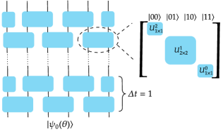
Figure 1: Random circuit with $6$ qubits. The initial state is chosen as the tilted ferromagnetic state and the blue rectangle represents random two-qubit gates in the even-odd brick-wall pattern. For the U(1) symmetric circuits, each two-qubit gate respects U(1) symmetry, resulting in a block diagonal structure for the unitary matrix of quantum gates.

As shown in Fig. 1, the initial state undergoes the unitary evolution of the random quantum circuits where two-qubit gates are arranged in a brick-wall structure. In the case of non-symmetric circuits, each two-qubit gate is randomly chosen from the Haar measure. For the U(1) symmetric case, the matrix for each two-qubit gate is block diagonal as shown in Fig. 1 and each block is randomly sampled from the Haar measure. One discrete time step $\Delta t=1$ includes two layers of two-qubit gates. We calculate the dynamics of entanglement asymmetry $\mathbb{E}[\Delta S_{A}]$ of subsystem $A$ averaged over different circuit configurations to monitor the dynamical and steady behaviors of symmetry restoration.

Symmetry restoration in the long-time limit.— We approximate the long-time limit of random circuit ensemble with a simpler ensemble $\mathbb{U}$ for a single random unitary $U$ acting on all qubits to compute Rényi-2 entanglement asymmetry [63, 64, 65, 66]. The approximation is justified as the analytical results from such global unitary approximation are consistent with numerical results for the average entanglement asymmetry under the evolution of long-time random U(1) symmetric circuits composed of local gates [6]. For the non-symmetric random circuit evolution, $\mathbb{U}$ constitutes a global $2$-design for the Haar measure. Consequently, the average Rényi-2 entanglement asymmetry at late time is [37]

$$\mathbb{E}[\Delta S_{A}^{(2)}]\approx-\log\left[\frac{1+2^{2|A|-N}/\sqrt{\pi|A|}}{1+2^{2|A|-N}}\right].$$ (3)

With large $N$, $\mathbb{E}[\Delta S_{A}^{(2)}]$ approches zero if $|A|<N/2$ while it sharply changes to a non-zero value $\log\sqrt{\pi|A|}$ if $|A|>N/2$. Therefore, the broken symmetry of subsystem $A$ with $|A|<N/2$ can always be restored by the non-symmetric random circuits at a late time, regardless of the choice of the initial state.

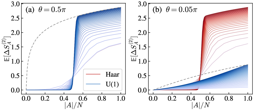
Figure 2: The average Rényi-2 entanglement asymmetry $\mathbb{E}[\Delta S^{(2)}_{A}]$ in the long-time limit of random circuit evolution starting from the tilted ferromagnetic initial states with the tilt angle (a) $\theta=0.5\pi$ and (b) $\theta=0.05\pi$ versus the subsystem size $|A|$. The increasing intensity of colors represents increasing system sizes $N\in\{8,12,\ldots,100\}$. The blue and red lines represent the results for U(1)-symmetric random circuits and random circuits without symmetry restriction, respectively. The grey dashed lines represent the entanglement asymmetry for the initial states.

For the U(1)-symmetric random circuit evolution, $\mathbb{U}$ is a global $2$-design for the composition of the Haar measures over each charge sector [64, 65, 66]. The average Rényi-2 entanglement asymmetry can be accurately obtained by calculating certain summations of polynomial numbers of binomial coefficient products, which arise from counting charge numbers [6]. As shown in Fig. 2, for the most asymmetric initial state with tilt angle $\theta=0.5\pi$, the steady state results from the non-symmetric evolution and U(1)-symmetric evolution coincide. However, as $\theta$ deviates from $0.5\pi$, notable disparities emerge between these two evolution settings. We note that $\mathbb{E}[\Delta S^{(2)}_{A}]$ of the steady state is always lower than that of the initial state in the case of U(1)-symmetric random circuit, while this is not necessarily true in the non-symmetric evolution. In this sense, non-symmetric random circuit evolution is featureless whereas symmetric random circuit evolution has an operational meaning of monotonically decreasing the asymmetry in the subsystem.

Figure 3: (a) The average Rényi-2 entanglement asymmetry $\mathbb{E}[\Delta S^{(2)}_{A}]$ in the long-time limit of U(1)-symmetric random circuit evolution at $|A|=N/4$ versus the tilt angle $\theta$. The increasing intensity of colors corresponds to $N\in\{8,12,\ldots,100\}$. The inset depicts the peak position $\theta_{\mathrm{max}}$ versus $N$. (b) The phase diagram for the symmetric restoration at $|A|<N/2$. The red and blue areas represent the symmetry-restored and persistent symmetry-breaking phases, respectively. The “critical point” $\theta_{c}\approx 2\theta_{\mathrm{max}}$ for the finite size crossover depends on $N$ with a $1/\sqrt{N}$ scaling.

Under the condition of large system size and large tilt angle, a simplified analytical form of $\mathbb{E}[\Delta S_{A}^{(2)}]$ can be obtained by approximating the binomial coefficients with the Gaussian distributions,

$$\mathbb{E}[\Delta S_{A}^{(2)}]\approx-\log\left[\frac{1+g(\theta)^{2|A|-N}/\sqrt{\pi|A|}}{1+g(\theta)^{2|A|-N}}\right],$$ (4)

which resembles the non-symmetric case in Eq. (3) except for the $\theta$-dependent base factor

$$g(\theta)=2\exp\left[-\frac{1}{2}\log^{2}\left(\tan^{2}\frac{\theta}{2}\right)\right].$$ (5)

If $\theta=0.5\pi$, Eq. (4) coincides with Eq. (3), giving an analytical explanation for the coincidence in Fig. 2(a). If the tilt angle remains large but deviates from $0.5\pi$, Eq. (4) indicates that the main characteristic remains unchanged compared with the non-symmetric case: the symmetry is restored for a small subsystem of $|A|<N/2$ but still broken for $|A|>N/2$.

However, if the tilt angle is small, the Gaussian approximation fails. We rely on direct estimation of the summations of binomial coefficients [6], which shows that for small tilt angles such as $\theta<0.1\pi$, $\mathbb{E}[\Delta S_{A}^{(2)}]$ will converge to a significant finite value in the long-time limit even for $|A|<N/2$ and large finite $N$. In other words, when the symmetry breaking in the tilted ferromagnetic initial state is relatively weak, it becomes challenging to fully restore the subsystem symmetry through the U(1)-symmetric random circuit evolution. Conversely, those initial states exhibiting more severe symmetry breaking can restore the symmetry successfully instead. This phenomenon is reminiscent of an extreme limit of the QME, where instead of restoring slowly, the symmetry does not fully restore for initial states with small symmetry breaking. As shown in Fig. 3, there exists a critical value $\theta_{c}$ where on the small-$\theta$ side the symmetry is not restored, leaving a persistent symmetry-breaking phase. It is worth noting that the above discussions only apply to the finite-size system as the critical value $\theta_{c}$ slowly varies with the system size $N$ with a scaling of $\theta_{c}\approx 1.13\pi/\sqrt{N}$.

Quantum Mpemba effect in early time dynamics.— Now we proceed to consider the entanglement asymmetry dynamics for different initial states with varying tilt angles $\theta$. The numerical simulations are performed using the TensorCircuit package [67]. We observe that the entanglement asymmetry decays more rapidly as the tilt angle increases for U(1) symmetric random quantum circuits, as illustrated in Fig. 4 (a). Namely, a QME emerges in the symmetry restoration process. It is important to highlight that the presence of QME depends on the choice of specific initial states and we observe the absence of QME when the tilted Néel state is chosen as the initial state as shown in Fig. 5 (b). Nevertheless, we emphasize that the presence of QMEs is not a fine-tuned phenomenon. We further investigate the entanglement asymmetry dynamics and observe QME with various sets of initial states, including tilted ferromagnetic states where the tilt angle on each qubit is randomly sampled from $[-W,W]$, which is more compatible with the experimental demonstration of QMEs on quantum devices since it doesn’t require high precision state preparation [6].

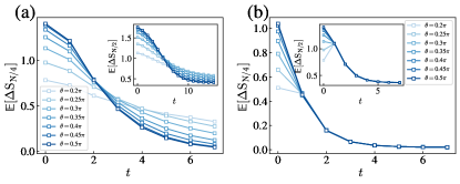
Figure 4: (a)(b) show the entanglement asymmetry dynamics of subsystem $A=[0,N/4]$ for random quantum circuits with and without U(1) symmetry respectively. We use $N=16$ in the former case and $N=8$ in the latter case. The insets show the results with subsystem $A=[0,N/2]$. QME exists for U(1) symmetric random circuits while it is absent in random circuits without any symmetry. Additionally, the entanglement asymmetry dynamics do not depend on the initial state in the latter case.

On the contrary, for non-symmetric random circuits, we observe a collapse in the entanglement asymmetry dynamics for various initial states, as depicted in Fig. 4 (b). Consequently, although the entanglement asymmetry still tends to zero at late times, the QME disappears trivially. This behavior can be understood in terms of the effective statistical model, where the initial state dependence has been eliminated as the inner product between different initial product states and the first layer of random unitary gates is constant [6].

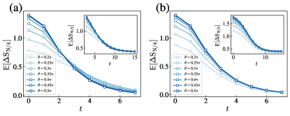
Figure 5: Entanglement asymmetry dynamics with the initial state as (a) tilted ferromagnetic state with a domain wall in the middle and (b) the tilted Néel state. In the former case, the QME is present, whereas it is absent in the latter case, although the late-time behaviors are the same for both initial states based on the analytical results.

Furthermore, we note that QME is captured by the early-time behaviors of the entanglement asymmetry dynamics, making the local spin configurations of the initial states crucial due to the casual cone structure. By contrast, the late-time behaviors only depend on the distribution over different charge sectors of the initial state [6]. As a result, the tilted Néel state and the tilted ferromagnetic state with a domain wall in the middle converge to the same steady state with the same entanglement asymmetry. However, QME is observed in the latter case while not in the former case, as shown in Fig. 5, as the latter initial state resembles the ferromagnetic state locally.

In addition, we have conducted investigations on setups that incorporate additional symmetries, such as spatial or temporal translational symmetry (random Floquet circuit) [68, 69, 70, 71]. We have found that thermalization accompanied by symmetry restoration and the QME persists in these setups as well [6]. Interestingly, the temporal translation symmetry slows down the symmetry restoration, consistent with the slow thermalization results in [70].

The unified mechanism behind the QME is that the thermalization speeds for different charge sectors are speculated to be different. Charge sectors with larger Hilbert space dimensions might show faster thermalization as indicated by the proxy results of entanglement asymmetry, while charge sectors with $O(1)$ dimension generally fail the ETH. Therefore, the criteria for the presence of QME is accordingly a suitable set of initial states where the extent of symmetry breaking is linked with the larger overlap with charge sectors of larger dimensions. Following such criteria for the initial states, more asymmetric initial states will thermalize faster with faster symmetry restoration. This crucial observation provides insights on the presence (absence) of QME for tilted ferromagnetic (Néel) states. For the tilted Néel initial state, more asymmetric states with larger $\theta$ deviate more from the largest charge $N/2$ sector and thermalize slower. Contrary to the QME, symmetry restoration is slower for more asymmetric initial states in this case.

Finally, we also investigate the symmetry restoration dynamics in quantum circuits with SU(2) and $Z_{2}$ symmetries. We extend the definition of entanglement asymmetry for SU(2) symmetry and identify the presence (absence) of QME in the SU(2) ($Z_{2}$) symmetric circuits [6]. The unified mechanism above also provides insights into these different internal symmetry cases. For $Z_{2}$ symmetry, there are only two equally large Hilbert subspaces, and the thermalization speeds of different initial states are expected to be similar with no QME. In the SU(2) symmetry case, the dimensions of different symmetry sectors vary from constant to exponential scaling like the U(1) case. Therefore, QME can be observed for designed initial states satisfying the criteria above.

Conclusions and discussions.— In this Letter, we have presented a rigorous and comprehensive theoretical analysis of subsystem symmetry restoration under the evolution of random quantum circuits respecting the U(1) symmetry. Our findings reveal that U(1)-symmetric circuits hinder the U(1) symmetry restoration when the input is a tilted ferromagnetic initial state with a small tilt angle $\theta$. Conversely, the symmetry can always be restored when the tilt angle is large, i.e., the initial state is more U(1)-asymmetric. These results highlight the distinctions between U(1)-symmetric and non-symmetric circuits in terms of symmetry restoration and quantum thermalization.

Besides the late-time analytical results, we have numerically investigated the early-time dynamics of symmetry restoration. Our results demonstrate the emergence of QME with specific initial states. We also provide a unified mechanism with the lens of quantum thermalization to understand the QME and successfully apply the understanding to the presence and absence of QME regarding different initial states and different internal symmetries including SU(2) and $Z_{2}$ symmetries.

Acknowledgement.— We acknowledge helpful discussions with Rui-An Chang, Zhou-Quan Wan, and Han Zheng. SL acknowledge the support during the visit to Sun Yat-sen University. S. Yin is supported by the National Natural Science Foundation of China (Grants No. 12075324 and No. 12222515) and the Science and Technology Projects in Guangdong Province (Grants No. 211193863020).

Supplemental Material for “Symmetry restoration and quantum Mpemba effect in symmetric random circuits”

I Symmetry properties of thermal equilibrium states

For a nonintegrable system under Hamiltonian $H$ with some conserved commuting or noncommuting charges $Q_{a}$, the thermal equilibrium state is given by quantum thermodynamics as [72, 73, 74, 75, 76, 77]

$$\rho_{th}=\frac{1}{Z}e^{-\beta(H-\sum_{a}\mu_{a}Q_{a})},$$ (S1)

where $Z$ is the partition function for normalization $Z=\text{Tr}(e^{-\beta(H-\sum_{a}\mu_{a}Q_{a})})$, and these coefficients of $\beta$ and $\mu$ are determined by the expectation value $E=\text{Tr}(\rho_{th}H)$ and $\langle Q_{a}\rangle=\text{Tr}(\rho_{th}Q_{a})$. When the charges are noncommuting as for non-Abelian symmetries of $H$, the equilibrium state is often referred as non-Abiliean thermal states (NATS) as the counterpart of generalized Gibbs ensemble (GGE) [78, 79, 80, 81, 82] for integrable systems.

If all charges $Q_{a}$ are commuting with each other, we can easily find a unitary transformation $U$ such that $U^{\dagger}|i\rangle=|Q_{a}=Q_{a}(i)\rangle$ which transforms the computational basis $|i\rangle$ into the common eigenstate of multiple charges $Q_{a}$. For example, for $Q=J_{z}$, $U=I$ already satisfies the requirement. The transformed density matrix gives

$$U\rho_{th}U^{\dagger}=\frac{1}{Z}e^{-\beta(UHU^{\dagger}-\sum_{a}\mu_{a}UQ_{a}U^{\dagger})}.$$ (S2)

The matrix on the exponential after the transformation is block diagonal for different charge sectors $\{Q_{a}\}$. We can show this by checking the matrix elements as $\langle i|UHU^{\dagger}|j\rangle=\langle Q_{a}=Q_{a}(i)|H|Q_{a}=Q_{a}(j)\rangle\propto\delta_{Q_{a}(i),Q_{a}(j)}$ and $\langle i|UQ_{a}U^{\dagger}|j\rangle=\langle Q_{a}=Q_{a}(i)|Q_{a}|Q_{a}=Q_{a}(j)\rangle=Q_{a}(i)\delta_{ij}$. The matrix exponential of the block diagonal matrix by charge sectors is still a block matrix of the same structure. Therefore, a thermal equilibrium state must admit a block diagonal structure on the basis of commuting charges (or equivalently, after applying the similar transformation $U$). Such a block diagonal structure is a manifestation of the symmetry restoration for corresponding charges. We thus conclude that symmetry restoration is a necessary condition for thermalization. Another way to understand the symmetry restoration in one dimensional system is provided by Mermin-Wagner-Hohenberg theorem [83, 84, 85]. The finite energy density of the initial symmetry-broken state acts as an effective non-zero temperature and leads to general symmetry restoration because the Mermin-Wagner-Hohenberg theorem forbids the spontaneous breaking of a symmetry at a finite temperature in 1D.

Now we focus on the noncommuting charges case. We use SU(2) symmetry as a representative example in the following analysis. Suppose we choose the $J_{z}$ direction arbitrarily and apply a similar procedure as the Abelian case, namely, we introduce $U^{\dagger}|i\rangle=|J,J_{z}\rangle$, where $J$ and $J_{z}$ is a set of good quantum numbers characterizing quantum states as the basis of SU(2) group irreducible representations. We now have $\langle i|UHU^{\dagger}|j\rangle\propto\delta_{J(i),J(j)}\delta_{J_{z}(i),J_{z}(j)}$ and $\langle i|UJ_{z}U^{\dagger}|j\rangle=J_{z}(i)\delta_{i,j}$. The two terms keep the expected block diagonal structure from SU(2) symmetry. However, $UJ_{x,y}U^{\dagger}$ has non-diagonal non-zero terms between states of different $J_{z}$, thus leaving the final density matrix with no explicit block diagonal structure.

To overcome the above issue, we need to find a better, more fine-grained transformation $U$, such that $U^{\dagger}|i\rangle=|J,J_{z}^{\prime}\rangle$. And now the $J_{z}^{\prime}$ direction is properly determined, such that we have $\text{Tr}(\rho_{th}J_{x^{\prime}})=\text{Tr}(\rho_{th}J_{y^{\prime}})=0$. We can decompose the new transformation $U$ as $U_{0}R$. $U_{0}$ is the same as the above paragraph, composed of CG coefficients, transforming the computational basis into the SU(2) irreducible representation basis $|J,J_{z}\rangle$. The newly introduced unitary matrix $R$ is effectively a rotation which can be defined as $R=e^{i\theta_{1}J_{x}}e^{i\theta_{2}J_{y}}$, rendering $\text{Tr}(\rho_{th}J_{x^{\prime}})=\text{Tr}(\rho_{th}J_{y^{\prime}})=0$ vanish. According to SM Section I in Ref. [76], this condition indicates that $\mu_{x}=\mu_{y}=0$, and the thermal state is now as:

$$U\rho_{th}U^{\dagger}=\frac{1}{Z}e^{-\beta(U_{0}HU_{0}^{\dagger}-\mu_{z}U_{0}J_{z}^{\prime}U_{0}^{\dagger})},$$ (S3)

with the expected block diagonal structure.

An equivalent perspective to understand the above transformation is that the chemical potentials $\mu_{a}$ transforms as an adjoint representation of SU(2), namely the SU(2) symmetry of the state is understood as $G(g)\rho_{th}(\vec{\mu})G^{\dagger}(g)=\rho_{th}(\text{ad}(g)\vec{\mu})$ where $g$ is the group element of SU(2) transformation and $G(g)$ is the corresponding representation operator ($R$ is an example of $G(g)$). $\text{ad}(g)$ is the adjoint representation of SU(2) ($J=1$ representation for SU(2), SO(3) faithful representation, 3D rotation). Instead, the trivial symmetry invariant definition for SU(2) symmetry $G(g)\rho_{th}G^{\dagger}(g)=\rho_{th}$ doesn’t work for the thermal equilibrium state [56], as it implies that $\text{Tr}(\rho_{th}\vec{J})=0$ which may not be compatible with the initial conditions. On the contrary, for the U(1) symmetry in the case of the commuting charges, each chemical potential is a scalar with respect to the corresponding symmetry operations, and $G(g)\rho_{th}G^{\dagger}(g)=\rho_{th}$ holds for $g\in U(1)$. This corresponds to the familiar definition of weak symmetry for mixed states $\rho_{th}$ which cannot directly apply to SU(2) symmetry case as we comment above. The difference lies in that SU(2) symmetry covariant state space is much larger than SU(2) symmetry invariant state space ($\langle J\rangle=0$).

Now, the density matrix after the transformation in Eq. (S3) keeps the block diagonal structure across different $\{J,J_{z}\}$ sectors and successfully manifests the SU(2) symmetry in the system dynamics. Again, symmetry restoration is also the necessary condition for the thermalization in this non-Abelian case.

In random circuit setups we detailed in the following sections, the effective $H=0$ is taken for a small subsystem. For a generic random Haar circuit, the final output state in the subsystem is a fully mixed state $I/2^{N}$. With U(1) symmetric random circuit, the subsystem density matrix will converge to $\rho\propto e^{-\mu J_{z}}$ at long times limit, as long as the initial state $\rho_{0}$ is generic and not solely or largely lie in the charge sectors of extreme values. The equilibrium density matrix for the subsystem can be numerically checked with Eq. (S28). This also explains why when the tilt angle $\theta$ is small on the ferromagnetic state, the symmetry restoration is very slow or even impossible for finite-size systems. The reason is that the initial state has a rather large overlap with $J_{z}=N$ sector of Hilbert space dimension $1$. Note that these $O(1)$ dimension sectors cannot thermalize as ETH doesn’t apply. Therefore, the state with small $\theta$ is slow in thermalization or fails to thermalize in finite-size systems. This also explains QME: QME is observed for the set of initial states, where the more symmetry is broken, the faster thermalization and thus faster symmetry restoration set in. For the SU(2) case, since the initial state already gives zero expectation on $J_{x}$, $J_{y}$, the final thermalized subsystem follows $\rho\propto e^{-\mu J_{z}}$ directly. In sum, in featureless random circuit cases, due to the lack of $H$, the final thermalized subsystems are all described by the diagonal matrix. This viewpoint also underlies our assumption that $Z_{2}$ symmetry cannot show QME behavior as each sector of $Z_{2}$ symmetry is exponentially large and equally easy to thermalize.

Specifically, for the initial states tested in SU(2) case in our work, we can directly verify that $\langle J_{x}\rangle=\langle J_{y}\rangle=0$ for even size subsystems and thus the natural direction of $J_{z}$ coincides with the preferred direction $J_{z}^{\prime}$, i.e. $R=I$, only $U_{0}$ transformation is required to reveal the symmetry structure of the evolved state.

II More numerical results for U(1) symmetric quantum circuits

II.1 With additional symmetries

In this section, we show more numerical results of the entanglement asymmetry dynamics with the same setup as that in the main text. In contrast to the previous results, the quantum circuits now possess additional symmetries beyond the U(1) symmetry. The initial state is chosen as the tilted ferromagnetic state as shown in Eq. 2. The numerical results with additional (discrete) spatial translation symmetry, temporal translation symmetry, and spatial and temporal translation symmetries are shown in Fig. S1 (a)(b)(c) respectively. In all these cases, QME still exists. Moreover, we find that the presence of temporal translation symmetry slows down the U(1) symmetry restoration and thermalization as shown in Fig. S1 (d). This is consistent with the results in Ref. [70] where U(1) symmetric random Haar Floquet circuit is reported to show slow thermalization.

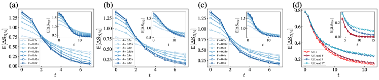
Figure S1: Entanglement asymmetry dynamics with additional (a) spatial translation symmetry (T), (b) temporal translation symmetry (F), and (c) spatial and temporal translation symmetries (FT). $A$ is set to $[0,N/4]$ and $[0,N/2]$ in the main panels and the insets with $N=16$, respectively. In (d), we show the comparison between entanglement asymmetry dynamics in the presence of additional symmetries with fixed tilt angle $\theta=0.2\pi$ in the main panel and $\theta=0.5\pi$ in the inset. The presence of temporal translation symmetry slows down the U(1) symmetry restoration.

II.2 With different initial states

Besides the three sets of initial states discussed in the main text: tilted ferromagnetic states, tilted Néel states, and tilted ferromagnetic states with a middle domain wall, we further investigate the entanglement asymmetry dynamics with initial states chosen as tilted ferromagnetic or Néel state with tilt angle on each qubit randomly sampled from $[-W,W]$. Although the existence of QME depends on the choice of the initial state, as shown in Fig. S2, QME still exits with an initial random tilted ferromagnetic state. The presence of QME from such initial states with randomness addresses the concern that QME is only specific to some fine-tuned states. And such initial states with random parameters are more suitable for experimental demonstration of QME on quantum devices because they do not require high-precision state preparation. In other words, the on-site randomness is irrelevant to the existence of QME.

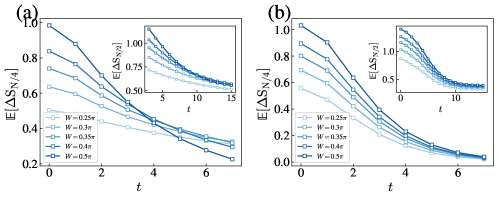
Figure S2: Entanglement asymmetry dynamics with initial (a) tilted ferromagnetic state and (b) tilted Néel state where tilt angle on each qubit is uniformly randomly sampled from $[-W,W]$. The QME exists in the former case while it is absent in the latter case, consistent with the results of uniform tilted angles.

Moreover, as mentioned in the main text, the entanglement asymmetry in the long time limit only depends on the distribution over different charge sectors of the initial states. Here, we numerically validate this prediction via the late-time entanglement asymmetry with initial states chosen as uniformly tilted Néel state and ferromagnetic state with a middle domain wall, the results are shown in Fig. S3.

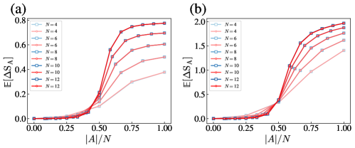
Figure S3: Entanglement asymmetry at late times with initial state chosen as tilted Néel state (red) and tilted ferromagnetic state with a middle domain wall (blue). The tilt angles are $\theta=\pi/10$ and $\theta=\pi/2$ for (a) and (b), respectively. These two initial states have the same late-time behaviors, although the early-time behaviors are significantly different.

II.3 Numerical results after a quench of global U(1) gate

In the analytical analysis, we have utilized a global U(1) symmetric unitary to approximate the brick-wall quantum circuits with sufficiently long depth. Here, we have numerically verified this approximation via the consistency check of Rényi-2 entanglement asymmetry at the late time of U(1) symmetric quantum circuits and after a quench of global U(1) symmetric gate, as shown in Fig. S4. Moreover, we have also verified the analytical results as discussed below with numerical results, as shown in Fig. S5.

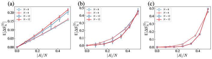
Figure S4: Rényi-2 entanglement asymmetry at the late time of U(1) symmetric quantum circuits composed of local gates (red) and after a quench of global U(1) symmetric unitary (blue) are consistent with each other as anticipated. The initial state is chosen as a tilted ferromagnetic state with tilt angles equaling $0.1\pi$, $0.3\pi$, and $0.5\pi$ for (a)(b)(c) respectively.

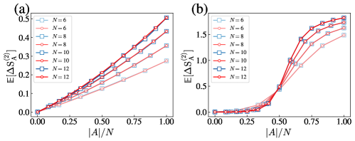
Figure S5: Rényi-2 entanglement asymmetry after a quench of global U(1) symmetric unitary obtained from numerical simulation (blue) and analytical form (red). The initial state is chosen as a tilted ferromagnetic state with the tilt angle equaling $0.1\pi$ and $0.5\pi$ for (a) and (b) respectively.

III Numerical results for other symmetric quantum circuits

III.1 $Z_{2}$ symmetric quantum circuits

In this section, we present the numerical results of entanglement asymmetry dynamics in the $Z_{2}$ symmetric quantum circuits. The symmetry operator of $Z_{2}$ symmetry is $\prod_{i}\sigma_{i}^{x}$ and $Z_{2}$ symmetric two-qubit gates are given by

$$U_{Z_{2}}=T^{{\dagger}}\begin{pmatrix}U_{+1}&0\\ 0&U_{-1}\end{pmatrix}T,$$ (S4)

where $U_{+1}$ and $U_{-1}$ are $2\times 2$ random Haar matrix corresponding to the $+1$ and $-1$ eigenbasis respectively, and $T$ is the transformation matrix from $Z_{2}$ symmetric basis to $z$ basis,

$$T=\begin{pmatrix}\frac{1}{\sqrt{2}}&0&0&\frac{1}{\sqrt{2}}\\ 0&\frac{1}{\sqrt{2}}&\frac{1}{\sqrt{2}}&0\\ 0&\frac{1}{\sqrt{2}}&\frac{-1}{\sqrt{2}}&0\\ \frac{1}{\sqrt{2}}&0&0&\frac{-1}{\sqrt{2}}\end{pmatrix}.$$ (S5)

We choose two different initial states: one is the tilted GHZ state given by

$$|\psi_{0}(\theta)\rangle=e^{-i\frac{\theta}{2}\sum_{j}\sigma^{y}_{j}}|\rm{GHZ}\rangle,$$ (S6)

where $|\rm{GHZ}\rangle=\frac{1}{\sqrt{2}}(|0\rangle^{\bigotimes N}+|1\rangle^{\bigotimes N})$. The other is the tilted ferromagnetic state. As shown in Fig. S6 (a)(b), there is no QME in the entanglement asymmetry dynamics of $Z_{2}$ symmetric quantum circuits. Moreover, we also calculate the entanglement asymmetry at late times. Different from the case of U(1) symmetric circuits with a tilted ferromagnetic state as the initial state, the $Z_{2}$ symmetry of subsystem $A$ with $|A|<N/2$ will always be restored, independent of the choice of initial states and tilt angles, as shown in Fig. S6 (c)(d).

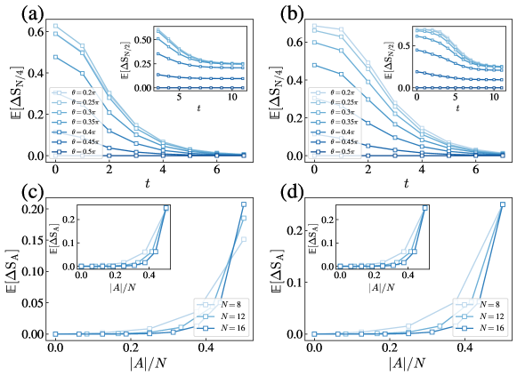
Figure S6: (a)(b) show the entanglement asymmetry dynamics of $Z_{2}$ symmetric circuits with $N=16$. (c)(d) show the entanglement asymmetry at late times versus subsystem size. The tilt angles are $\theta=0.1\pi$ and $\theta=0.2\pi$ in the main panel and the inset. The initial state is the tilted GHZ state and the tilted ferromagnetic state for (a)(c) and (b)(d) respectively.

III.2 SU(2) symmetric quantum circuits

In the main text, we have demonstrated that the QME emerges in the entanglement asymmetry dynamics of U(1) symmetric quantum circuits. Here, we show numerical results for the SU(2) symmetric quantum circuits. The initial state is chosen as the tilted ferromagnetic state with staggered tilt angles, i.e.,

$$|\psi_{0}(\theta)\rangle=e^{-i\frac{\theta}{2}\sum_{j}(-1)^{j}\sigma_{j}^{y}}|000...0\rangle.$$ (S7)

We can directly verify that $\langle J_{x}\rangle=\langle J_{y}\rangle=0$ for even size subsystems and thus the natural direction of $z$ coincides with the preferred direction $z^{\prime}$ for the block diagonalization of the equilibrium density matrix. Therefore, the SU(2) symmetry restoration indicates that the reduced density matrix is block-diagonal corresponding to the $\{J^{2},J_{z}\}$ sectors. However, we emphasize that the block-diagonal structure is only a necessary but not sufficient condition for the non-Abelian symmetric density matrix because the Schur lemma also requires there is some equivalence among different sectors when the dimension of the irreducible representation is larger than $1$. Namely, different from the case of Abelian symmetries, the zero entanglement asymmetry does not necessarily mean that the quantum state respects the corresponding non-Abelian symmetry. In sum, vanishing entanglement asymmetry with repect to SU(2) symmetry is a necessary condition for SU(2) symmetry restoration and SU(2) symmetry restoration is a necessary condition for quantum thermalization. Therefore, we can still use the entanglement asymmetry as an indicator of the symmetry restoration and thermalization for the non-Abelian symmetries. The numerical results are shown in Fig. S7. We also observe the QME in the entanglement asymmetry dynamics as anticipated by the unified mechanism we developed in the main text.

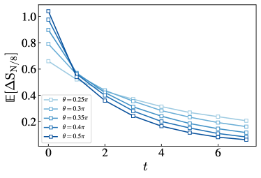
Figure S7: Entanglement asymmetry dynamics of SU(2) symmetric quantum circuits with the presence of QME. Here $N=16$. The initial state is a tilted ferromagnetic state with staggered tilt angles.

IV Analytical Results

In this section, we provide the analytical results for the dynamical and steady behaviors of entanglement asymmetry under the evolution of random quantum circuits with and without U(1) symmetry.

IV.1 Calculation without symmetry in the early time

As shown in the main text, the entanglement asymmetry dynamics collapse for different initial states for random circuits without any symmetry. To understand this phenomenon, we can consider the average of random two-qubit gates,

$$\mathbb{E}_{\mathcal{U}}(U_{t,(i,i+1)}\otimes U_{t,(i,i+1)}^{*})^{\otimes 2}=\sum_{\sigma,\tau\in S_{2}}\text{Wg}_{d^{2}}^{(2)}(\sigma\tau^{-1})|\tau\tau\rangle\langle\sigma\sigma|_{i,i+1},$$ (S8)

where $S_{2}=\{I,S\}$ with $I=\sum_{ij}|iijj\rangle$ and $S=\sum_{ij}|ijji\rangle$ being the elements from $S_{2}$ permutation group. The initial ferromagnetic state can be written as $|\psi_{0}(\theta)\rangle=\bigotimes_{i}\psi_{0}^{i}(\theta)$ where $|\psi_{0}^{i}(\theta)\rangle=\cos\frac{\theta}{2}|0\rangle_{i}+\sin\frac{\theta}{2}|1\rangle_{i}$. The reduced density matrix in the two-copy replicated Hilbert space is

$$|\rho_{i}\rangle=(\cos^{2}\frac{\theta}{2}|00\rangle+\cos\frac{\theta}{2}\sin\frac{\theta}{2}|01\rangle+\cos\frac{\theta}{2}\sin\frac{\theta}{2}|10\rangle+\sin^{2}\frac{\theta}{2}|11\rangle)^{\otimes 2}.$$ (S9)

Thus,

$$\langle I|\rho_{i}\rangle=\langle S|\rho_{i}\rangle=1.$$ (S10)

Therefore, the output state of the first layer of random two-qubit gates does not depend on the initial state, and the entanglement asymmetry dynamics collapse for different initial states. In fact, this conclusion still holds as long as the initial state is a product state.
 

Next, we provide the analytical results for the dynamics of entanglement asymmetry under the evolution of random quantum circuits with and without U(1) symmetry in the long-time limit.

IV.2 Calculation without symmetry in the long-time limit

Suppose the evolution time is sufficiently long, e.g. polynomial with the system size. In that case, the circuit ensemble can usually be approximated by a single Haar-random unitary acting on all qubits at least for the second moment in Rényi-2 entanglement asymmetry [63]. We denote this “global” random unitary as $U$ and the corresponding ensemble as $\mathbb{U}$. Suppose $\rho_{0}$ is a pure initial state and $\rho=U^{\dagger}\rho_{0}U$ is the resulting randomly evolved state. Denote the reduced density matrix of subsystem $A$ as $\rho_{A}=\tr_{\bar{A}}(\rho)$, where $\bar{A}$ is the complement region of $A$. We use $|A|$ to represent the number of qubits in the subsystem $A$. The total number of qubits is denoted as $N$.

If there is no symmetry restriction at all, then $\mathbb{U}$ just means the Haar measure on the whole Hilbert space. The corresponding detailed calculation can be found in Ref. [37]. Here we reproduce the same results using an alternative method, which facilitates the derivation of the U(1)-symmetric case below. As we know, the purity of $\rho_{A}$ can be written as the expectation of a certain SWAP operator with respect to the 2-fold replica of $\rho$, i.e.,

$$\tr(\rho_{A}^{2})=\tr_{2A}(\rho_{A}^{\otimes 2}S|_{2A})=\tr_{2A}[\tr_{2\bar{A}}(\rho^{\otimes 2})S|_{2A}]=\tr[\rho^{\otimes 2}(S|_{2A}\otimes I|_{2\bar{A}})],$$ (S11)

where $S|_{2A}$ and $I|_{2\bar{A}}$ are the SWAP operator and the identity on the 2-fold replicas of subsystem $A$ and $\bar{A}$, respectively. The corresponding tensor network diagram is

$$\leavevmode\hbox to76.92pt{\vbox to76.53pt{\text{[drawing]}}}\quad.$$ (S12)

Using the formula from the Weingarten calculus [86], the average of the 2-fold replica of the Haar-random state is

$$\mathbb{E}_{\mathbb{U}}[\rho^{\otimes 2}]=\mathbb{E}_{\mathbb{U}}[U^{\dagger\otimes 2}\rho_{0}^{\otimes 2}U^{\otimes 2}]=\frac{(\tr\rho_{0})^{2}I+\tr(\rho_{0}^{2})S}{d^{2}-1}-\frac{(\tr\rho_{0})^{2}S+\tr(\rho_{0}^{2})I}{d(d^{2}-1)}=\frac{I+S}{d(d+1)},$$ (S13)

where we have used the fact that $\rho_{0}$ is a pure state. Here $d=2^{N}$ denotes the Hilbert space dimension of the entire system. Hence, the average of the purity of $\rho_{A}$ is

$$\mathbb{E}_{\mathbb{U}}[\tr(\rho_{A}^{2})]=\tr[\frac{(I+S)}{d(d+1)}(S|_{2A}\otimes I|_{2\bar{A}})]=\frac{d_{A}d_{\bar{A}}^{2}+d_{\bar{A}}d_{A}^{2}}{d(d+1)}=\frac{d_{\bar{A}}+d_{A}}{d+1}=\frac{2^{|\bar{A}|}+2^{|A|}}{2^{N}+1},$$ (S14)

where $d_{A}$ and $d_{\bar{A}}$ denote the Hilbert space dimensions of subsystem $A$ and $\bar{A}$ respectively. Next, we consider the “pruned” reduced state [24]

$$\rho_{A,Q}=\sum_{q=0}^{|A|}\Pi_{q}|_{A}\rho_{A}\Pi_{q}|_{A},$$ (S15)

where $\Pi_{q}|_{A}$ is the projector on the charge sector of $q$ charges restricted to subsystem $A$. Namely, $\rho_{A,Q}$ is the result of removing all non-zero elements outside the block-diagonal structure of charge sectors in $\rho_{A}$. The purity of $\rho_{A,Q}$ can be written as

$$\tr(\rho_{A,Q}^{2}) =\sum_{q=0}^{|A|}\tr\left[\Pi_{q}|_{A}\rho_{A}\Pi_{q}|_{A}\rho_{A}\Pi_{q}|_{A}\right]=\sum_{q=0}^{|A|}\tr\left[\rho^{\otimes 2}((\Pi_{q}|_{A})^{\otimes 2}S|_{2A})\otimes I|_{2\bar{A}}\right].$$ (S16)

The tensor network diagram corresponding to a single term in the summation is

$$\leavevmode\hbox to76.92pt{\vbox to76.53pt{\text{[drawing]}}}\quad,$$ (S17)

where the orange blocks represent the projector $\Pi_{q}|_{A}$. Substitute the expectation $\mathbb{E}_{\mathbb{U}}[\rho^{\otimes 2}]$ and we obtain

$$\mathbb{E}_{\mathbb{U}}[\tr(\rho_{A,Q}^{2})] =\sum_{q}\tr\left[\mathbb{E}_{\mathbb{U}}[\rho^{\otimes 2}]((\Pi_{q}|_{A})^{\otimes 2}S|_{2A})\otimes I|_{2\bar{A}}\right]$$ (S18)

$$=\sum_{q=0}^{|A|}\tr\left[\frac{I+S}{d(d+1)}((\Pi_{q}|_{A})^{\otimes 2}S|_{2A})\otimes I|_{2\bar{A}})\right]$$

$$=\sum_{q=0}^{|A|}\frac{d_{\bar{A}}^{2}}{d(d+1)}\tr\left[(\Pi_{q}|_{A})^{2}\right]+\frac{d_{\bar{A}}}{d(d+1)}\tr\left[(\Pi_{q}|_{A})^{\otimes 2}\right]$$

$$=\frac{d_{\bar{A}}^{2}}{d(d+1)}\sum_{q=0}^{|A|}\binom{|A|}{q}+\frac{d_{\bar{A}}}{d(d+1)}\sum_{q=0}^{|A|}\binom{|A|}{q}^{2}$$

$$=\frac{d_{A}d_{\bar{A}}^{2}}{d(d+1)}+\frac{d_{\bar{A}}}{d(d+1)}\binom{2|A|}{|A|}$$

$$=\frac{1}{2^{N}+1}\left[2^{|\bar{A}|}+\frac{(2|A|)!}{2^{|A|}(|A|!)^{2}}\right],$$

where we have used a special case of Vandermonde’s identity, i.e., the summation of the squared binomial coefficients chosen from $n$ equals the central binomial coefficient chosen from $2n$. The ensemble average of the $2$-degree Rényi entanglement asymmetry, i.e., the difference between the $2$-degree Rényi entropies of the pruned state and the original state, can be approximated by the negative logarithm of the ratio of the two average purities above for the sake of the concentration of measure [37]

$$\Delta S_{A}^{(2)} =S_{2}(\rho_{A,Q})-S_{2}(\rho_{A})\approx-\log\frac{\mathbb{E}_{\mathbb{U}}[\tr(\rho_{A,Q}^{2})]}{\mathbb{E}_{\mathbb{U}}[\tr(\rho_{A}^{2})]}$$ (S19)

$$=-\log\left[\frac{1}{1+2^{2|A|-N}}\left(1+\frac{(2|A|)!}{2^{N}(|A|!)^{2}}\right)\right]$$

$$\approx-\log\left[\frac{1}{1+2^{2|A|-N}}\left(1+\frac{4^{|A|}}{2^{N}\sqrt{\pi|A|}}\right)\right]$$

$$=-\log\left[\frac{1+4^{|A|-N/2}/\sqrt{\pi|A|}}{1+4^{|A|-N/2}}\right].$$

One can see that in the large size limit $N\rightarrow\infty$, $\mathbb{E}[\Delta S_{A}^{(2)}]$ is almost zero when $|A|<N/2$ and sharply changes to a non-zero value $\log\sqrt{\pi|A|}$ when $|A|>N/2$.

IV.3 Calculation with U(1) symmetry in the long-time limit

Next, we consider the random circuits with the global U(1)-symmetry restriction. That is to say, every gate in the circuit should commute with the on-site symmetry operator $e^{-iZ_{j}\theta}$, i.e.,

$$\leavevmode\hbox to24.4pt{\vbox to31.7pt{\text{[drawing]}}}\quad=\quad\leavevmode\hbox to24.4pt{\vbox to31.7pt{\text{[drawing]}}}\quad,$$ (S20)

where the blue square represents the given gate and the red circles represent the Pauli-Z rotation gates. To construct the ensemble $\mathbb{U}$ that respects a certain symmetry, one reasonable choice is to assemble the Haar measures over each subspace of irreducible representation (irrep) for that symmetry. That is to say, under the eigenbasis of the symmetry, we require each sub-block to be an independent Haar-random unitary, i.e.,

$$\mathbb{U}=\left\{U\mid U=\bigoplus_{q}(U_{q}\otimes I_{q}),~{}U_{q}\text{ is Haar-random}\right\},$$ (S21)

where $q$ is the label of irreps. $I_{q}$ is the identity of dimension $d_{q}$ in a single irrep of $q$. $U_{q}$ is a unitary of dimension $r_{q}$ on the tensor-product-quotient space of the $r_{q}$ repeated irreps of $q$. The symmetric ensemble $\mathbb{U}$ is defined by taking each $U_{q}$ as an independent Haar-random matrix.

For the global U(1) symmetry, $q$ just corresponds to the total charge number $\hat{Q}=\sum_{i}n_{i}$ or say the total spin $z$-component $\sum_{i}\sigma^{z}_{i}$. As the U(1) group is Abelian, its irreps are all one-dimensional $d_{q}=1$, which are just the phase factors with different frequencies $e^{iq\theta}$. The number of repeated irreps of $q$ equals the number of occupation configurations corresponding to $q$ charges on $N$ sites, i.e., $r_{q}=\binom{N}{q}$. For simplicity, we replace the direct sum by a normal sum with projectors

$$\mathbb{U}=\left\{U\mid U=\sum_{q}U_{q}\Pi_{q}\right\},$$ (S22)

where $\Pi_{q}$ is the projector onto the subspace of $q$, i.e., the $q$-charge sector. Note that $\Pi_{q}$ corresponds to the subspace of all the repeated irreps of $q$, instead of just one of them. Compared to Eq. (S21), $U_{q}$ in Eq. (S22) is enlarged to the whole Hilbert space by padding identities. Under the eigenbasis of the symmetry, $U_{q}$ and $\Pi_{q}$ take the form of

$$U_{q}=\left(\begin{matrix}*&0\\ 0&I\end{matrix}\right),\quad\Pi_{q}=\left(\begin{matrix}I&0\\ 0&0\end{matrix}\right),$$ (S23)

where the upper left block represents the $q$-charge sector and the lower right block represents the others. Hence we naturally have $U_{q}\Pi_{q}=\Pi_{q}U_{q}$. In other words, $U_{q}\Pi_{q}$ can be seen as a pseudo-unitary padded with zeros outside the $q$-charge sector. We will denote

$$V_{q}=U_{q}\Pi_{q}$$ (S24)

for simplicity below.

We start from the first-order integration. Since Haar averaging requires that each unitary is paired with its conjugation (otherwise the integral vanishes), the first-order integration over the U(1)-symmetric ensemble $\mathbb{U}$ becomes

$$\mathbb{E}_{\mathbb{U}}\left[\rho\right] =\mathbb{E}_{\mathbb{U}}\left[U^{\dagger}\rho_{0}U\right]=\mathbb{E}_{\mathbb{U}}\left[\left(\sum_{q}V_{q}^{\dagger}\right)\rho_{0}\left(\sum_{q^{\prime}}V_{q^{\prime}}\right)\right]$$ (S25)

$$=\sum_{qq^{\prime}}\mathbb{E}_{\mathbb{U}}\left[V_{q}^{\dagger}\rho_{0}V_{q^{\prime}}\right]=\sum_{q}\mathbb{E}_{\mathbb{U}}\left[V_{q}^{\dagger}\rho_{0}V_{q}\right]$$

$$=\sum_{q}\mathbb{E}_{\mathbb{U}}\left[U_{q}^{\dagger}\Pi_{q}\rho_{0}\Pi_{q}U_{q}\right]=\sum_{q}\frac{\tr(\Pi_{q}\rho_{0}\Pi_{q})}{r_{q}}\Pi_{q}=\sum_{q}\frac{\tr(\rho_{0}\Pi_{q})}{r_{q}}\Pi_{q}.$$

One can see that the result is almost the maximally mixed state but with different weights on different charge sectors, which respects the weak symmetry $e^{i\hat{Q}\theta}\mathbb{E}_{\mathbb{U}}\left[\rho\right]e^{-i\hat{Q}\theta}=\mathbb{E}_{\mathbb{U}}\left[\rho\right]$. Moreover, if the initial state $\rho_{0}$ respects the strong symmetry $e^{i\hat{Q}\theta}\rho_{0}=e^{iq\theta}\rho_{0}$, i.e., the non-zero elements in $\rho_{0}$ is within a single charge sector, then Eq. (S25) tells us that the evolved state will be the “maximally mixed state” within the $q$-charge sector, which still respects the strong symmetry, exhibiting the charge conservation law of the evolution.

After partially tracing out subsystem $\bar{A}$, the result is still a diagonal matrix under the computational basis, implying that the averaged reduced density matrix $\mathbb{E}_{\mathbb{U}}[\rho_{A}]$ must also respect the weak symmetry. To be specific, by definition, we know the projector $\Pi_{q}$ can be decomposed as

$$\Pi_{q}=\sum_{q^{\prime}=0}^{q}\Pi_{q^{\prime}}|_{A}\otimes\Pi_{q-q^{\prime}}|_{\bar{A}},$$ (S26)

where $\Pi_{q^{\prime}}|_{A}$ denotes the projector to the $q^{\prime}$ charge subspace restricted on the subsystem $A$. By default, we assume if $q^{\prime}>|A|$ then $\Pi_{q^{\prime}}|_{A}=0$. Hence the index $q^{\prime}$ actually takes values from $\max\{0,q-|\bar{A}|\}$ to $\min\{q,|A|\}$ in Eq. (S26). The partial trace of the projector is

$$\tr_{\bar{A}}\Pi_{q}=\sum_{q^{\prime}}\Pi_{q^{\prime}}|_{A}\tr(\Pi_{q-q^{\prime}}|_{\bar{A}})=\sum_{q^{\prime}=0}^{q}\binom{|\bar{A}|}{q-q^{\prime}}\Pi_{q^{\prime}}|_{A}.$$ (S27)

We denote $\binom{n}{k}=0$ if $k>n$. Hence, the averaged reduced density matrix is

$$\mathbb{E}_{\mathbb{U}}[\rho_{A}]=\mathbb{E}_{\mathbb{U}}[\tr_{\bar{A}}\rho]=\sum_{q}\frac{\tr(\Pi_{q}\rho_{0}\Pi_{q})}{r_{q}}\tr_{\bar{A}}\Pi_{q}=\sum_{q^{\prime}q}\frac{\tr(\rho_{0}\Pi_{q})}{r_{q}}\binom{|\bar{A}|}{q-q^{\prime}}\Pi_{q^{\prime}}|_{A},$$ (S28)

One can see that the result depends on the initial state $\rho_{0}$ only via the factor $\tr(\rho_{0}\Pi_{q})$. If the initial state takes the form of the $Y$-tilted ferromagnetic state

$$e^{-\frac{i}{2}\sum_{j}\sigma^{y}_{j}\theta}\ket{0}^{\otimes N}=\left(\cos\frac{\theta}{2}\ket{0}-\sin\frac{\theta}{2}\ket{1}\right)^{\otimes N}=\sum_{b}\left(\cos\frac{\theta}{2}\right)^{N-q(b)}\left(-\sin\frac{\theta}{2}\right)^{q(b)}\ket{b},$$ (S29)

where $b$ represents $01$-bit strings and $q(b)$ counts the number of $1$ in $b$, then the weight in the $q$-charge sector is

$$\tr(\rho_{0}\Pi_{q}) =\sum_{b}\left(\cos^{2}\frac{\theta}{2}\right)^{N-q(b)}\left(\sin^{2}\frac{\theta}{2}\right)^{q(b)}\langle b|\Pi_{q}|b\rangle$$ (S30)

$$=\sum_{b}\left(\cos^{2}\frac{\theta}{2}\right)^{N-q(b)}\left(\sin^{2}\frac{\theta}{2}\right)^{q(b)}\delta_{q(b),q}$$

$$=r_{q}\left(\cos^{2}\frac{\theta}{2}\right)^{N-q}\left(\sin^{2}\frac{\theta}{2}\right)^{q}.$$

The averaged reduced density matrix hence becomes

$$\mathbb{E}_{\mathbb{U}}[\rho_{A}] =\sum_{q^{\prime}=0}^{|A|}\sum_{q=q^{\prime}}^{q^{\prime}+|\bar{A}|}\left(\cos^{2}\frac{\theta}{2}\right)^{N-q}\left(\sin^{2}\frac{\theta}{2}\right)^{q}\binom{|\bar{A}|}{q-q^{\prime}}\Pi_{q^{\prime}}|_{A}$$ (S31)

$$=\left(\cos^{2}\frac{\theta}{2}\right)^{|A|}\sum_{q^{\prime}=0}^{|A|}\left(\tan^{2}\frac{\theta}{2}\right)^{q^{\prime}}\Pi_{q^{\prime}}|_{A},$$

where the summation over $(q-q^{\prime})$ is simply the expansion of the binomial $\left(\cos^{2}\frac{\theta}{2}+\sin^{2}\frac{\theta}{2}\right)^{|\bar{A}|}$. One can see that when $\theta\rightarrow 0$ or $\theta\rightarrow\pi$, the weights concentrate on the $q^{\prime}=0$ or $q^{\prime}=|A|$ charge sector, consistent with the fact that the initial all-zero / all-one state will not be changed and thus not thermalize by the U(1)-symmetric evolution. When $\theta\in(0,\pi/2)$, the weights form an exponential distribution decaying from $q^{\prime}=0$ to $q^{\prime}=|A|$ with the decaying rate $-\log\left(\tan^{2}\frac{\theta}{2}\right)$. Similarly, when $\theta\in(\pi/2,\pi)$, the weights also form an exponential distribution but decaying from $q^{\prime}=|A|$ to $q^{\prime}=0$. If $\theta=\pi/2$, the weights are uniform, i.e., the averaged reduced density matrix becomes exactly the maximally mixed state. It is worth noticing that the results depend on the initial state $\rho_{0}$ only through the initial distribution over different charge sectors, i.e., the factor $\tr(\rho_{0}\Pi_{q})$. The same is true for the second-order integration below.

Next, we consider the second-order integration. According to the conjugation-pair rule of Haar averaging, the second-order integration can be expanded as

$$\mathbb{E}_{\mathbb{U}}\left[U^{\dagger\otimes 2}AU^{\otimes 2}\right] =\mathbb{E}_{\mathbb{U}}\left[\left(\sum_{q}V_{q}^{\dagger}\right)^{\otimes 2}A\left(\sum_{q^{\prime}}V_{q^{\prime}}\right)^{\otimes 2}\right]=\sum_{qpq^{\prime}p^{\prime}}\mathbb{E}_{\mathbb{U}}\left[(V_{q}^{\dagger}\otimes V_{p}^{\dagger})A(V_{q^{\prime}}\otimes V_{p^{\prime}})\right]$$ (S32)

$$=\sum_{q\neq p}\mathbb{E}_{\mathbb{U}}\left[(V_{q}^{\dagger}\otimes V_{p}^{\dagger})A(V_{q}\otimes V_{p})\right]+\mathbb{E}_{\mathbb{U}}\left[(V_{q}^{\dagger}\otimes V_{p}^{\dagger})A(V_{p}\otimes V_{q})\right]$$

$$\quad+\sum_{q}\mathbb{E}_{\mathbb{U}}\left[(V_{q}^{\dagger}\otimes V_{q}^{\dagger})A(V_{q}\otimes V_{q})\right].$$

The first term can be integrated as

$$\sum_{q\neq p}\mathbb{E}_{\mathbb{U}}\left[(V_{q}^{\dagger}\otimes V_{p}^{\dagger})A(V_{q}\otimes V_{p})\right]=\sum_{q\neq p}\frac{\tr[A(\Pi_{q}\otimes\Pi_{p})]}{r_{q}r_{p}}\Pi_{q}\otimes\Pi_{p}.$$ (S33)

The second term can be integrated as

$$\sum_{q\neq p}\mathbb{E}_{\mathbb{U}}\left[(V_{q}^{\dagger}\otimes V_{p}^{\dagger})A(V_{p}\otimes V_{q})\right]=\sum_{q\neq p}\frac{\tr[AS(\Pi_{q}\otimes\Pi_{p})]}{r_{q}r_{p}}(\Pi_{q}\otimes\Pi_{p})S,$$ (S34)

where $S$ is the SWAP operator on the two replicas. The third term can be integrated as

$$\sum_{q}\mathbb{E}_{\mathbb{U}}\left[(V_{q}^{\dagger}\otimes V_{q}^{\dagger})A(V_{q}\otimes V_{q})\right]$$ (S35)

$$=\sum_{q}\left[\frac{\tr(A\Pi_{q}^{\otimes 2})I+\tr(SA\Pi_{q}^{\otimes 2})S}{r_{q}^{2}-1}-\frac{\tr(A\Pi_{q}^{\otimes 2})S+\tr(SA\Pi_{q}^{\otimes 2})I}{r_{q}(r_{q}^{2}-1)}\right]\Pi_{q}^{\otimes 2}.$$

If we take $A=\rho_{0}^{\otimes 2}$, then the above three terms in $\mathbb{E}_{\mathbb{U}}[\rho^{\otimes 2}]$ reduce to

$$\sum_{q\neq p}\mathbb{E}_{\mathbb{U}}\left[(V_{q}^{\dagger}\otimes V_{p}^{\dagger})\rho_{0}^{\otimes 2}(V_{q}\otimes V_{p})\right]=\sum_{q\neq p}\frac{\tr(\rho_{0}\Pi_{q})\tr(\rho_{0}\Pi_{p})}{r_{q}r_{p}}\Pi_{q}\otimes\Pi_{p},$$ (S36)

$$\sum_{q\neq p}\mathbb{E}_{\mathbb{U}}\left[(V_{q}^{\dagger}\otimes V_{p}^{\dagger})\rho_{0}^{\otimes 2}(V_{p}\otimes V_{q})\right] =\sum_{q\neq p}\frac{\tr(\rho_{0}\Pi_{q}\rho_{0}\Pi_{p})}{r_{q}r_{p}}(\Pi_{q}\otimes\Pi_{p})S$$ (S37)

$$=\sum_{q\neq p}\frac{\tr(\rho_{0}\Pi_{q})\tr(\rho_{0}\Pi_{p})}{r_{q}r_{p}}(\Pi_{q}\otimes\Pi_{p})S,$$

$$\sum_{q}\mathbb{E}_{\mathbb{U}}\left[(V_{q}^{\dagger}\otimes V_{q}^{\dagger})\rho_{0}^{\otimes 2}(V_{q}\otimes V_{q})\right]$$ (S38)

$$=\sum_{q}\left[\frac{\tr(\rho_{0}\Pi_{q})^{2}I+\tr((\rho_{0}\Pi_{q})^{2})S}{r_{q}^{2}-1}-\frac{\tr(\rho_{0}\Pi_{q})^{2}S+\tr((\rho_{0}\Pi_{q})^{2})I}{r_{q}(r_{q}^{2}-1)}\right]\Pi_{q}^{\otimes 2}$$

$$=\sum_{q}\frac{\tr(\rho_{0}\Pi_{q})^{2}}{r_{q}(r_{q}+1)}(I+S)\Pi_{q}^{\otimes 2},$$

where we have used the fact that $\rho_{0}$ is a pure state so that $\tr(\rho_{0}^{2})=1$ and

$$\tr(\rho_{0}\Pi_{q}\rho_{0}\Pi_{p})=\tr(\rho_{0}\Pi_{q})\tr(\rho_{0}\Pi_{p}),$$ (S39)

$$\tr((\rho_{0}\Pi_{q})^{2})=(\tr(\rho_{0}\Pi_{q}))^{2}.$$

Hence, the expectation of the purity of $\rho_{A}$ is

$$\mathbb{E}_{\mathbb{U}}[\tr(\rho_{A}^{2})]=\tr\left[\mathbb{E}_{\mathbb{U}}[\rho^{\otimes 2}](S|_{2A}\otimes I|_{2\bar{A}})\right]$$ (S40)

$$=\sum_{q\neq p}\frac{\tr(\rho_{0}\Pi_{q})\tr(\rho_{0}\Pi_{p})}{r_{q}r_{p}}\left[\tr(\tr_{\bar{A}}\Pi_{q}\tr_{\bar{A}}\Pi_{p})+\tr(\tr_{A}\Pi_{q}\tr_{A}\Pi_{p})\right]$$

$$\quad+\sum_{q}\frac{\tr(\rho_{0}\Pi_{q})^{2}}{r_{q}(r_{q}+1)}\left[\tr((\tr_{\bar{A}}\Pi_{q})^{2})+\tr((\tr_{A}\Pi_{q})^{2})\right].$$

The involved trace factors can be calculated as

$$\tr(\tr_{\bar{A}}\Pi_{q}\tr_{\bar{A}}\Pi_{p}) =\sum_{q^{\prime}p^{\prime}}\binom{|\bar{A}|}{q-q^{\prime}}\binom{|\bar{A}|}{p-p^{\prime}}\tr(\Pi_{q^{\prime}}|_{A}\Pi_{p^{\prime}}|_{A})$$ (S41)

$$=\sum_{q^{\prime}}\binom{|\bar{A}|}{q-q^{\prime}}\binom{|\bar{A}|}{p-q^{\prime}}\binom{|A|}{q^{\prime}}$$

$$=\sum_{q^{\prime}=0}^{\min\{q,p\}}\binom{|\bar{A}|}{q-q^{\prime}}\binom{|\bar{A}|}{p-q^{\prime}}\binom{|A|}{q^{\prime}}$$

$$\equiv f(q,p,|A|,|\bar{A}|),$$

$$\tr(\tr_{A}\Pi_{q}\tr_{A}\Pi_{p}) =f(q,p,|\bar{A}|,|A|),$$ (S42)

$$\tr((\tr_{\bar{A}}\Pi_{q})^{2}) =f(q,q,|A|,|\bar{A}|),$$ (S43)

$$\tr((\tr_{A}\Pi_{q})^{2}) =f(q,q,|\bar{A}|,|A|),$$ (S44)

Remember that $\binom{n}{k}=0$ if $k>n$ and hence the index $q^{\prime}$ actually takes values from $\max\{0,q-|\bar{A}|,p-|\bar{A}|\}$ to $\min\{q,p,|A|\}$ in the definition of $f(q,p,|A|,|\bar{A}|)$ in Eq. (S41). If the initial state takes the form of the $Y$-tilted ferromagnetic state, the two coefficients in Eq. (S40) become

$$\frac{\tr(\rho_{0}\Pi_{q})\tr(\rho_{0}\Pi_{p})}{r_{q}r_{p}}=\left(\cos^{2}\frac{\theta}{2}\right)^{2N-q-p}\left(\sin^{2}\frac{\theta}{2}\right)^{q+p},$$ (S45)

$$\frac{\tr(\rho_{0}\Pi_{q})^{2}}{r_{q}(r_{q}+1)}=\frac{r_{q}}{r_{q}+1}\left(\cos^{2}\frac{\theta}{2}\right)^{2N-2q}\left(\sin^{2}\frac{\theta}{2}\right)^{2q}.$$

Thus, the average purity of $\rho_{A}$ becomes

$$\mathbb{E}_{\mathbb{U}}[\tr(\rho_{A}^{2})]=\sum_{q\neq p}\left(\cos^{2}\frac{\theta}{2}\right)^{2N-q-p}\left(\sin^{2}\frac{\theta}{2}\right)^{q+p}[f(q,p,|A|,|\bar{A}|)+f(q,p,|\bar{A}|,|A|)]$$ (S46)

$$\quad+\sum_{q}\frac{r_{q}}{r_{q}+1}\left(\cos^{2}\frac{\theta}{2}\right)^{2N-2q}\left(\sin^{2}\frac{\theta}{2}\right)^{2q}\left[f(q,q,|A|,|\bar{A}|)+f(q,q,|\bar{A}|,|A|)\right].$$

On the other hand, the purity of the pruned reduced state is

$$\tr(\rho_{A,Q}^{2}) =\tr\left(\sum_{qp}\Pi_{q}|_{A}\rho_{A}\Pi_{q}|_{A}\Pi_{p}|_{A}\rho_{A}\Pi_{p}|_{A}\right)$$ (S47)

$$=\sum_{q}\tr\left(\rho_{A}\Pi_{q}|_{A}\rho_{A}\Pi_{q}|_{A}\right)$$

$$=\sum_{q}\tr\left[\rho^{\otimes 2}((\Pi_{q}|_{A})^{\otimes 2}S|_{2A})\otimes I_{2\bar{A}}\right].$$

Thus the average purity of the pruned state is

$$\mathbb{E}_{\mathbb{U}}[\tr(\rho_{A,Q}^{2})] =\sum_{q^{\prime}}\tr\left[\mathbb{E}_{\mathbb{U}}[\rho^{\otimes 2}]((\Pi_{q^{\prime}}|_{A})^{\otimes 2}S|_{2A})\otimes I|_{2\bar{A}}\right]$$ (S48)

$$=\sum_{q\neq p,q^{\prime}}\frac{\tr(\rho_{0}\Pi_{q})\tr(\rho_{0}\Pi_{p})}{r_{q}r_{p}}\bigg{[}\tr\big((\tr_{\bar{A}}\Pi_{q})(\Pi_{q^{\prime}}|_{A})(\tr_{\bar{A}}\Pi_{p})(\Pi_{q^{\prime}}|_{A})\big{missing})$$

$$\quad\quad\quad\quad\quad\quad+\tr(\tr_{A}(\Pi_{q}(\Pi_{q^{\prime}}|_{A}))\tr_{A}(\Pi_{p}(\Pi_{q^{\prime}}|_{A})))\bigg{]}$$

$$\quad+\sum_{q,q^{\prime}}\frac{\tr(\rho_{0}\Pi_{q})^{2}}{r_{q}(r_{q}+1)}\left[\tr(((\tr_{\bar{A}}\Pi_{q})(\Pi_{q^{\prime}}|_{A}))^{2})+\tr((\tr_{A}(\Pi_{q}(\Pi_{q^{\prime}}|_{A})))^{2})\right].$$

The subterms take the form of

$$\tr\big((\tr_{\bar{A}}\Pi_{q})(\Pi_{q^{\prime}}|_{A})(\tr_{\bar{A}}\Pi_{p})(\Pi_{q^{\prime}}|_{A})\big{missing}) =\binom{|\bar{A}|}{q-q^{\prime}}\binom{|\bar{A}|}{p-q^{\prime}}\binom{|A|}{q^{\prime}},$$ (S49)

$$\tr(\tr_{A}(\Pi_{q}(\Pi_{q^{\prime}}|_{A}))\tr_{A}(\Pi_{p}(\Pi_{q^{\prime}}|_{A}))) =\binom{|A|}{q^{\prime}}\binom{|A|}{q^{\prime}}\binom{|\bar{A}|}{q-q^{\prime}}\delta_{pq},$$ (S50)

$$\tr(((\tr_{\bar{A}}\Pi_{q})(\Pi_{q^{\prime}}|_{A}))^{2}) =\binom{|\bar{A}|}{q-q^{\prime}}\binom{|\bar{A}|}{q-q^{\prime}}\binom{|A|}{q^{\prime}},$$ (S51)

$$\tr((\tr_{A}(\Pi_{q}(\Pi_{q^{\prime}}|_{A})))^{2}) =\binom{|A|}{q^{\prime}}\binom{|A|}{q^{\prime}}\binom{|\bar{A}|}{q-q^{\prime}}.$$ (S52)

Hence, the average purity of $\rho_{A,Q}$ becomes

$$\mathbb{E}_{\mathbb{U}}[\tr(\rho_{A,Q}^{2})]=\sum_{q\neq p}\left(\cos^{2}\frac{\theta}{2}\right)^{2N-q-p}\left(\sin^{2}\frac{\theta}{2}\right)^{q+p}f(q,p,|A|,|\bar{A}|)$$ (S53)

$$\quad+\sum_{q}\frac{r_{q}}{r_{q}+1}\left(\cos^{2}\frac{\theta}{2}\right)^{2N-2q}\left(\sin^{2}\frac{\theta}{2}\right)^{2q}\left[f(q,q,|A|,|\bar{A}|)+f(q,q,|\bar{A}|,|A|)\right].$$

One can see that Eq. (S53) is almost the same as Eq. (S46), except missing the term involving $f(q,p,|\bar{A}|,|A|)$. The Rényi entanglement asymmetry can be obtained by substituting Eqs. (S46) and (S53) into

$$\Delta S_{A}^{(2)}=S_{2}(\rho_{A,Q})-S_{2}(\rho_{A})\approx-\log\frac{\mathbb{E}_{\mathbb{U}}[\tr(\rho_{A,Q}^{2})]}{\mathbb{E}_{\mathbb{U}}[\tr(\rho_{A}^{2})]}.$$ (S54)

According to Eqs. (S46) and (S53), both $\mathbb{E}_{\mathbb{U}}[\tr(\rho_{A,Q}^{2})]$ and $\mathbb{E}_{\mathbb{U}}[\tr(\rho_{A}^{2})]$ are just sums of a polynomial number of certain binomial coefficients, which can be easily and accurately calculated numerically. But unfortunately, the symbolic summation of these binomial coefficients will lead to generalized hypergeometric functions, which are hard to write in an explicit closed form. However, in the large-size limit $N\rightarrow\infty$, the distribution of binomial coefficients converges to the Gaussian distribution and the summations can be well approximated by continuum integrals under certain conditions, which can give rise to a simple and meaningful analytical form of $\mathbb{E}[\Delta S_{A}^{(2)}]$. To be specific, we first regard $\frac{r_{q}}{r_{q}+1}\approx 1$ (recall $r_{q}=\binom{N}{q}$). This makes $\mathbb{E}_{\mathbb{U}}[\tr(\rho_{A,Q}^{2})]$ and $\mathbb{E}_{\mathbb{U}}[\tr(\rho_{A}^{2})]$ reduce to

$$\mathbb{E}_{\mathbb{U}}[\tr(\rho_{A}^{2})] \approx\left(\cos^{2}\frac{\theta}{2}\right)^{2N}\sum_{q,p}\left(\tan^{2}\frac{\theta}{2}\right)^{q+p}[f(q,p,|A|,|\bar{A}|)+f(q,p,|\bar{A}|,|A|)].$$ (S55)

$$\mathbb{E}_{\mathbb{U}}[\tr(\rho_{A,Q}^{2})] \approx\left(\cos^{2}\frac{\theta}{2}\right)^{2N}\sum_{q,p}\left(\tan^{2}\frac{\theta}{2}\right)^{q+p}[f(q,p,|A|,|\bar{A}|)+f(q,p,|\bar{A}|,|A|)\delta_{qp}].$$ (S56)

One can find that up to this approximation, the only difference between the two terms is the Kronecker factor $\delta_{qp}$. Suppose $|A|$ and $|\bar{A}|$ grow linearly with $N$ in the large size limit. We use the Gaussian distribution to approximate the binomial coefficients

$$\binom{n}{k}\approx\frac{2^{n}}{\sqrt{\pi n/2}}\exp\left[-\frac{(k-n/2)^{2}}{n}\right].$$ (S57)

Then the function $f(q,p,|A|,|\bar{A}|)$ can be approximated by

$$f(q,p,|A|,|\bar{A}|)=\sum_{q^{\prime}=0}^{\min\{q,p\}}\binom{|\bar{A}|}{q-q^{\prime}}\binom{|\bar{A}|}{p-q^{\prime}}\binom{|A|}{q^{\prime}}$$ (S58)

$$\approx\frac{2^{2|\bar{A}|+|A|}}{\sqrt{\pi^{3}|\bar{A}|^{2}|A|/8}}\int dq^{\prime}\exp\left[-\frac{(q-q^{\prime}-|\bar{A}|/2)^{2}}{|\bar{A}|}-\frac{(p-q^{\prime}-|\bar{A}|/2)^{2}}{|\bar{A}|}-\frac{(q^{\prime}-|A|/2)^{2}}{|A|}\right]$$

$$=\frac{2^{2|\bar{A}|+|A|}}{\sqrt{\pi^{3}|\bar{A}|^{2}|A|/8}}\sqrt{\frac{\pi|A||\bar{A}|}{2|A|+|\bar{A}|}}\times$$

$$\quad\exp\left[-\frac{|A|^{2}|\bar{A}|+2|A|\left(|\bar{A}|^{2}+(p-q)^{2}-|\bar{A}|(p+q)\right)+|\bar{A}|\left(|\bar{A}|^{2}-2|\bar{A}|(p+q)+2(p^{2}+q^{2})\right)}{2|\bar{A}|(2|A|+|\bar{A}|)}\right]$$

$$\equiv\tilde{f}(q,p,|A|,|\bar{A}|).$$

By use of Gaussian integration, the two summations can be approximated by

$$\sum_{q,p}\left(\tan^{2}\frac{\theta}{2}\right)^{q+p}f(q,p,|A|,|\bar{A}|)\approx\int dqdp\left(\tan^{2}\frac{\theta}{2}\right)^{q+p}\tilde{f}(q,p,|A|,|\bar{A}|)$$ (S59)

$$=\frac{2^{2|\bar{A}|+|A|}}{\sqrt{\pi^{3}|\bar{A}|^{2}|A|/8}}\sqrt{\pi^{3}|A||\bar{A}|^{2}}\exp\left[2(2|A|+|\bar{A}|)\log^{2}\left|\tan\frac{\theta}{2}\right|\right]\left(\tan^{2}\frac{\theta}{2}\right)^{2(|A|+|\bar{A}|)}$$

$$=2^{N+|\bar{A}|}\sqrt{8}\exp\left[2(N+|A|)\log^{2}\left|\tan\frac{\theta}{2}\right|\right]\left(\tan^{2}\frac{\theta}{2}\right)^{N},$$

and

$$\sum_{q}\left(\tan^{2}\frac{\theta}{2}\right)^{2q}f(q,q,|A|,|\bar{A}|)\approx\int(\sqrt{2}dq)\left(\tan^{2}\frac{\theta}{2}\right)^{2q}\tilde{f}(q,q,|A|,|\bar{A}|)$$ (S60)

$$=\frac{2^{2|\bar{A}|+|A|}}{\sqrt{\pi^{3}|\bar{A}|^{2}|A|/8}}\sqrt{2}\sqrt{\pi^{2}|A||\bar{A}|/2}\exp\left[2(2|A|+|\bar{A}|)\log^{2}\left|\tan\frac{\theta}{2}\right|\right]\left(\tan^{2}\frac{\theta}{2}\right)^{2(|A|+|\bar{A}|)}$$

$$=2^{N+|\bar{A}|}\sqrt{\frac{8}{\pi|\bar{A}|}}\exp\left[2(N+|A|)\log^{2}\left|\tan\frac{\theta}{2}\right|\right]\left(\tan^{2}\frac{\theta}{2}\right)^{N},$$

where the $\sqrt{2}$ factor in the integration measure in Eq. (S60) arises because the integral domain of Eq. (S60) is the diagonal line on the $p$-$q$ plane compared to Eq. (S59). To make the integration results above valid and meaningful, they should satisfy $\mathbb{E}_{\mathbb{U}}[\tr(\rho_{A}^{2})]\leq 1$ and $\mathbb{E}_{\mathbb{U}}[\tr(\rho_{A,Q}^{2})]\leq 1$ especially for $N\rightarrow\infty$, which will give rise to extra restrictions on $\theta$. For example, if we take $|A|=|\bar{A}|=N/2$, then the restriction is

$$2^{3/2}\times\exp\left[3\log^{2}\left|\tan\frac{\theta}{2}\right|\right]\left(\cos^{2}\frac{\theta}{2}\right)\left(\sin^{2}\frac{\theta}{2}\right)\leq 1\Rightarrow\frac{\pi}{2}-0.128\pi\leq\theta\leq\frac{\pi}{2}+0.128\pi,$$ (S61)

which means that this approximation can only be valid around $\theta=\frac{\pi}{2}$. This can be understood by the fact that when $\theta$ is too small, the factor $(\tan^{2}\frac{\theta}{2})^{q+p}$ in Eqs. (S55) and (S56) will concentrate at the margin $q+p=0$, where the error of the Gaussian approximation is relatively large. Moreover, if one wants the approximated purity to be valid for arbitrary values of $|A|$, the extreme restriction will occur at $|\bar{A}|=0$ or $|A|=0$, i.e.,

$$4\times\exp\left[2\log^{2}\left|\tan\frac{\theta}{2}\right|\right]\left(\cos^{2}\frac{\theta}{2}\right)\left(\sin^{2}\frac{\theta}{2}\right)\leq 1\Rightarrow\theta=\frac{\pi}{2}.$$ (S62)

Namely the Gaussian approximation is valid only at a single point $\theta=\frac{\pi}{2}$ if we consider arbitrary values of $|A|$ simultaneously. However, we will see below that the final result is actually reasonable in a finite region of $\theta$ around $\frac{\pi}{2}$. Substituting the integration results, the Rényi-2 entanglement asymmetry becomes

$$\Delta S_{A}^{(2)} \approx-\log\frac{\mathbb{E}_{\mathbb{U}}[\tr(\rho_{A,Q}^{2})]}{\mathbb{E}_{\mathbb{U}}[\tr(\rho_{A}^{2})]}$$ (S63)

$$\approx-\log\frac{2^{|\bar{A}|}\exp\left[2|A|\log^{2}\left|\tan\frac{\theta}{2}\right|\right]+2^{|A|}\exp\left[2|\bar{A}|\log^{2}\left|\tan\frac{\theta}{2}\right|\right]/\sqrt{\pi|A|}}{2^{|\bar{A}|}\exp\left[2|A|\log^{2}\left|\tan\frac{\theta}{2}\right|\right]+2^{|A|}\exp\left[2|\bar{A}|\log^{2}\left|\tan\frac{\theta}{2}\right|\right]}$$

$$=-\log\frac{1+2^{|A|-|\bar{A}|}\exp\left[-2(|A|-|\bar{A}|)\log^{2}\left|\tan\frac{\theta}{2}\right|\right]/\sqrt{\pi|A|}}{1+2^{|A|-|\bar{A}|}\exp\left[-2(|A|-|\bar{A}|)\log^{2}\left|\tan\frac{\theta}{2}\right|\right]}$$

$$=-\log\frac{1+g(\theta)^{|A|-|\bar{A}|}/\sqrt{\pi|A|}}{1+g(\theta)^{|A|-|\bar{A}|}},$$

where $|A|-|\bar{A}|=2|A|-N=2N(|A|/N-1/2)$ and

$$g(\theta)=2\exp\left[-2\log^{2}\left|\tan\frac{\theta}{2}\right|\right].$$ (S64)

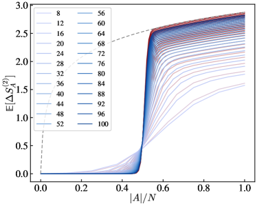
Figure S8: The average Rényi-2 entanglement asymmetry $\mathbb{E}[\Delta S^{(2)}_{A}]$ in the long-time limit of U(1)-symmetric random circuit evolution with the tilt angle $\theta=0.4\pi$ from the ferromagnetic initial state versus the subsystem size $|A|$. The numbers in the legend represent different system sizes $N$. The blue and red lines represent the results from U(1)-symmetric circuits and non-symmetric circuits, respectively. The grey dashed line represents the result for the tilted ferromagnetic initial state.

Note that $g(\theta)=2$ for $\theta=\frac{\pi}{2}$ and $g(\theta)\geq 1$ for $\theta-\frac{\pi}{2}\in[-0.17\pi,0.17\pi]$. Within this range, the expression above indicates that in the large size limit $N\rightarrow\infty$, $\Delta S_{A}^{(2)}\rightarrow 0$ if $|A|<N/2$ and $\Delta S_{A}^{(2)}\rightarrow\log\sqrt{\pi|A|}$ if $|A|>N/2$, quite similar to the result Eq. (S19) in the case of non-symmetric evolution except that the base factor $g(\theta)$ can deviate from $2$. The validity of Eq. (S63) can be verified by numerically computing the summations of binomial coefficients in Eqs. (S46) and (S53). As shown in Fig. 2 of the main text, if $\theta=0.5\pi$, the results almost coincide with the non-symmetric case, consistent with the approximated analytical results Eq. (S63) and Eq. (S19). If $\theta$ slightly deviates from $\frac{\pi}{2}$, e.g., $\theta=0.4\pi$, as shown in Fig. S8, the overall magnitude of the curves is decreased but the main shape and trend remain qualitatively unchanged.

A feature significantly different from the case of non-symmetric random circuits is that the average Rényi-2 entanglement asymmetry of the final state in the case of U(1)-symmetric random circuits is always lower than that of the initial state, regardless of the value of $|A|$, as shown by the blue curves in Fig. 2 and Figs. S8-S10. This is not necessarily true in the case of non-symmetric random circuits, as shown by the red curves in the corresponding figures, where the average entanglement asymmetry of the final state is the same for any initial state, allowing situations where the entanglement asymmetry of the final state is larger than that of the initial state. In this sense, non-symmetric random circuit evolution is featureless, whereas symmetric random circuit evolution holds a meaningful physical interpretation, i.e., it only leads to the restoration of the symmetry without further breaking the symmetry.

In addition, when $\theta$ slightly deviates from $\frac{\pi}{2}$, the factor $\log^{2}\left|\tan\frac{\theta}{2}\right|$ deviates from $0$ and hence $g(\theta)$ decreases from $2$. If $|A|<N/2$, then $g(\theta)^{|A|-|\bar{A}|}$ will increase and hence the late time $\mathbb{E}[\Delta S_{A}^{(2)}]$ will increase. On the other hand, for the initial tilted state, when $\theta$ decreases from $\frac{\pi}{2}$ to $0$, the U(1)-symmetry breaking is weakened, and the entanglement asymmetry $\mathbb{E}[\Delta S_{A}^{(2)}]$ will decrease. The inverse order of $\mathbb{E}[\Delta S_{A}^{(2)}]$ at the beginning and the end of the evolution suggests that there must exist cross points among the evolution curves with different $\theta$, consistent with the quantum Mpemba effect observed in the numerical experiments.

If $\theta$ deviates too much from $\frac{\pi}{2}$, or say $\theta$ is close to $0$, e.g., $\theta<0.33\pi$, then the Gaussian approximation above fails and there is no direct analytical evidence for the symmetry restoration at $|A|<N/2$. Direct numerical estimation using Eqs. (S46) and (S53) shows that for small tilt angles such as $\theta<0.1\pi$, $\mathbb{E}[\Delta S_{A}^{(2)}]$ will converge to a significant finite value in the long-time limit for large but finite system size $N$. As shown in Fig. 2 of the main text, when $\theta=0.05\pi$, $\mathbb{E}[\Delta S_{A}^{(2)}]$ increases with the system size for any $|A|$ up to $N=100$, which is very different from the large-$\theta$ case where $\mathbb{E}[\Delta S_{A}^{(2)}]$ decreases with $N$ at $|A|<N/2$. This fact implies that if the symmetry breaking in the tilted ferromagnetic initial state is too weak, it will be hard to fully restore the symmetry by the U(1)-symmetric random circuit evolution, while those initial states with more severe symmetry breaking can successfully restore the symmetry by contrast. This is somehow an extreme case of the quantum Mpemba effect, i.e., instead of restoring slowly, the symmetry does not restore at all for initial states with small symmetry breaking. It is worth noting that the above discussion is restricted to the finite-size system with uniformly tilted ferromagnetic initial states.

Nevertheless, the increase of $\mathbb{E}[\Delta S_{A}^{(2)}]$ with $N$ in the small-$\theta$ case will not last to the thermodynamic limit. This can be seen from Fig. S10 where $\mathbb{E}[\Delta S_{A}^{(2)}]$ at $|A|<N/2$ increases with $N$ first and then decreases. This non-monotonic behavior will be more clear in Fig. 3 of the main text, where we fix $|A|=N/4$ to see the curve of $\mathbb{E}[\Delta S_{A}^{(2)}]$ versus $\theta$ for different $N$. We can see that for $0.2\pi\lesssim\theta\leq 0.5\pi$, $\mathbb{E}[\Delta S_{A}^{(2)}]$ decreases monotonically with $N$ very fast down to zero while for $\theta\lesssim 0.2\pi$, $\mathbb{E}[\Delta S_{A}^{(2)}]$ will first increase and then decreases with $N$, and converges to zero very slowly for a relatively large $N$.

Importantly, one can see a prominent peak in Fig. textcolorLinkColor3 of the main text, whose position is denoted as $\theta_{\mathrm{max}}$ below, gradually shifts towards $\theta=0$ as $N$ increases while the height of the peak is almost constant. Around this peak at $\theta_{\mathrm{max}}$, $\mathbb{E}[\Delta S_{A}^{(2)}]$ takes significant finite values while is very close to zero away from this peak. The left end of this peak is just $\theta=0$. The right end of this peak can be properly defined as $\theta_{c}=2\theta_{\mathrm{max}}$. In other words, $\theta_{c}$ serves as a critical point where on the small-$\theta$ side the symmetry is not fully restored (persistent symmetry-breaking phase) while on the large-$\theta$ side, the symmetry is restored (symmetry-restored phase). A schematic finite-size crossover phase diagram is shown in Fig. 3 of the main text.

However, the “symmetry breaking phase” is not a true phase in the sense of the thermodynamic limit because $\theta_{c}$, albeit slowly, scales with the system size $N$ in the scaling of $1/\sqrt{N}$, as shown in the inset of Fig. 3. That is to say, in the thermodynamic limit, regardless of the value of the tilt angle $\theta$, the subsystem symmetry will always be restored for $|A|<N/2$ which is consistent with the eigenstate thermalization hypothesis. But conversely, for any finite-size system, there always exists a “critical point" $\theta_{c}\approx 1.13\pi/\sqrt{N}$, such that the subsystem symmetry cannot be restored for tilted ferromagnetic initial state with $\theta<\theta_{c}$.

It is worth mentioning that this lack of symmetry restoration is only observed in slightly tilted ferromagnetic initial states. As a counterexample, for tilted Néel states, the subsystem symmetry will always be restored by the U(1)-symmetric random circuit at late time as long as $|A|<N/2$ regardless of the tilt angle. This can be attributed to the fact that the Néel state is in the largest symmetry sector of exponentially large dimensions, while the ferromagnetic state is in a small symmetry sector of one dimension in the $\theta=0$ limit.

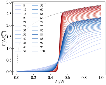
Figure S9: The average Rényi-2 entanglement asymmetry $\mathbb{E}[\Delta S^{(2)}_{A}]$ in the long-time limit of U(1)-symmetric random circuit evolution with the tilt angle $\theta=0.2\pi$ from the ferromagnetic initial state versus the subsystem size $|A|$. The numbers in the legend represent different system sizes $N$. The blue and red lines represent the results from U(1)-symmetric circuits and non-symmetric circuits, respectively. The grey dashed line represents the result for the tilted ferromagnetic initial state.

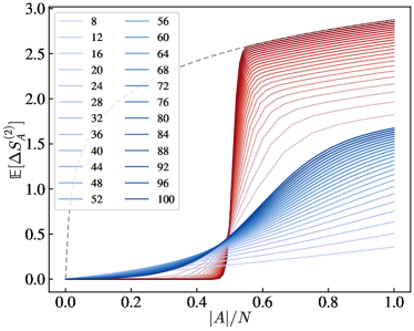
Figure S10: The average Rényi-2 entanglement asymmetry $\mathbb{E}[\Delta S^{(2)}_{A}]$ in the long-time limit of U(1)-symmetric random circuit evolution with the tilt angle $\theta=0.1\pi$ from the ferromagnetic initial state versus the subsystem size $|A|$. The numbers in the legend represent different system sizes $N$. The blue and red lines represent the results from U(1)-symmetric circuits and non-symmetric circuits, respectively. The grey dashed line represents the result for the tilted ferromagnetic initial state.

References

- Deutsch [1991] J. M. Deutsch, Quantum statistical mechanics in a closed system, Phys. Rev. A 43, 2046 (1991).
- Srednicki [1994] M. Srednicki, Chaos and quantum thermalization, Phys. Rev. E 50, 888 (1994).
- D’Alessio et al. [2016] L. D’Alessio, Y. Kafri, A. Polkovnikov, and M. Rigol, From quantum chaos and eigenstate thermalization to statistical mechanics and thermodynamics, Advances in Physics 65, 239 (2016).
- Rigol et al. [2008] M. Rigol, V. Dunjko, and M. Olshanii, Thermalization and its mechanism for generic isolated quantum systems, Nature 452, 854 (2008).
- Deutsch [2018] J. M. Deutsch, Eigenstate thermalization hypothesis, Reports on Progress in Physics 81, 082001 (2018).
- Note [1] See the Supplemental Material for more details, including (I) symmetry properties of thermal equilibrium states; (II) more numerical results for symmetric quantum circuits; (III) numerical results for other symmetric quantum circuits; (IV) analytical results.
- Mpemba and Osborne [1979] E. B. Mpemba and D. G. Osborne, The mpemba effect, Physics Education 14, 410 (1979).
- Lasanta et al. [2017] A. Lasanta, F. Vega Reyes, A. Prados, and A. Santos, When the hotter cools more quickly: Mpemba effect in granular fluids, Phys. Rev. Lett. 119, 148001 (2017).
- Lu and Raz [2017] Z. Lu and O. Raz, Nonequilibrium thermodynamics of the markovian mpemba effect and its inverse, Proceedings of the National Academy of Sciences 114, 5083 (2017).
- Klich et al. [2019] I. Klich, O. Raz, O. Hirschberg, and M. Vucelja, Mpemba index and anomalous relaxation, Phys. Rev. X 9, 021060 (2019).
- Kumar and Bechhoefer [2020] A. Kumar and J. Bechhoefer, Exponentially faster cooling in a colloidal system, Nature 584, 64 (2020).
- Bechhoefer et al. [2021] J. Bechhoefer, A. Kumar, and R. Chétrite, A fresh understanding of the Mpemba effect, Nature Reviews Physics 3, 534 (2021).
- Teza et al. [2023] G. Teza, R. Yaacoby, and O. Raz, Relaxation shortcuts through boundary coupling, Phys. Rev. Lett. 131, 017101 (2023).
- Kumar et al. [2022] A. Kumar, R. Chétrite, and J. Bechhoefer, Anomalous heating in a colloidal system, Proceedings of the National Academy of Sciences 119, e2118484119 (2022).
- Nava and Fabrizio [2019] A. Nava and M. Fabrizio, Lindblad dissipative dynamics in the presence of phase coexistence, Phys. Rev. B 100, 125102 (2019).
- Carollo et al. [2021] F. Carollo, A. Lasanta, and I. Lesanovsky, Exponentially accelerated approach to stationarity in markovian open quantum systems through the mpemba effect, Phys. Rev. Lett. 127, 060401 (2021).
- Manikandan [2021] S. K. Manikandan, Equidistant quenches in few-level quantum systems, Phys. Rev. Res. 3, 043108 (2021).
- Kochsiek et al. [2022] S. Kochsiek, F. Carollo, and I. Lesanovsky, Accelerating the approach of dissipative quantum spin systems towards stationarity through global spin rotations, Phys. Rev. A 106, 012207 (2022).
- Ivander et al. [2023] F. Ivander, N. Anto-Sztrikacs, and D. Segal, Hyperacceleration of quantum thermalization dynamics by bypassing long-lived coherences: An analytical treatment, Phys. Rev. E 108, 014130 (2023).
- Chatterjee et al. [2023a] A. K. Chatterjee, S. Takada, and H. Hayakawa, Quantum mpemba effect in a quantum dot with reservoirs, Phys. Rev. Lett. 131, 080402 (2023a).
- Chatterjee et al. [2023b] A. K. Chatterjee, S. Takada, and H. Hayakawa, Multiple quantum mpemba effect: exceptional points and oscillations, arXiv:2311.01347 (2023b).
- Wang and Wang [2024] X. Wang and J. Wang, Mpemba effects in nonequilibrium open quantum systems, arXiv:2401.14259 (2024).
- Shapira et al. [2024] S. A. Shapira, Y. Shapira, J. Markov, G. Teza, N. Akerman, O. Raz, and R. Ozeri, The mpemba effect demonstrated on a single trapped ion qubit, arXiv:2401.05830 (2024).
- Ares et al. [2023a] F. Ares, S. Murciano, and P. Calabrese, Entanglement asymmetry as a probe of symmetry breaking, Nature Communications 14, 2036 (2023a).
- Fagotti et al. [2014] M. Fagotti, M. Collura, F. H. L. Essler, and P. Calabrese, Relaxation after quantum quenches in the spin- heisenberg xxz chain, Phys. Rev. B 89, 125101 (2014).
- Polkovnikov et al. [2011] A. Polkovnikov, K. Sengupta, A. Silva, and M. Vengalattore, Colloquium: Nonequilibrium dynamics of closed interacting quantum systems, Rev. Mod. Phys. 83, 863 (2011).
- Calabrese et al. [2016] P. Calabrese, F. H. L. Essler, and G. Mussardo, Introduction to ‘Quantum Integrability in Out of Equilibrium Systems’, Journal of Statistical Mechanics: Theory and Experiment 2016, 064001 (2016).
- Vidmar and Rigol [2016] L. Vidmar and M. Rigol, Generalized gibbs ensemble in integrable lattice models, Journal of Statistical Mechanics: Theory and Experiment 2016, 064007 (2016).
- Essler and Fagotti [2016] F. H. L. Essler and M. Fagotti, Quench dynamics and relaxation in isolated integrable quantum spin chains, Journal of Statistical Mechanics: Theory and Experiment 2016, 064002 (2016).
- Doyon [2020] B. Doyon, Lecture notes on Generalised Hydrodynamics, SciPost Phys. Lect. Notes , 18 (2020).
- Bastianello et al. [2022] A. Bastianello, B. Bertini, B. Doyon, and R. Vasseur, Introduction to the special issue on emergent hydrodynamics in integrable many-body systems, Journal of Statistical Mechanics: Theory and Experiment 2022, 014001 (2022).
- Alba et al. [2021] V. Alba, B. Bertini, M. Fagotti, L. Piroli, and P. Ruggiero, Generalized-hydrodynamic approach to inhomogeneous quenches: correlations, entanglement and quantum effects, Journal of Statistical Mechanics: Theory and Experiment 2021, 114004 (2021).
- Fagotti [2014] M. Fagotti, On conservation laws, relaxation and pre-relaxation after a quantum quench, Journal of Statistical Mechanics: Theory and Experiment 2014, P03016 (2014).
- Bertini and Fagotti [2015] B. Bertini and M. Fagotti, Pre-relaxation in weakly interacting models, Journal of Statistical Mechanics: Theory and Experiment 2015, P07012 (2015).
- Ares et al. [2023b] F. Ares, S. Murciano, E. Vernier, and P. Calabrese, Lack of symmetry restoration after a quantum quench: An entanglement asymmetry study, SciPost Phys. 15, 089 (2023b).
- Joshi et al. [2024] L. K. Joshi, J. Franke, A. Rath, F. Ares, S. Murciano, F. Kranzl, R. Blatt, P. Zoller, B. Vermersch, P. Calabrese, et al., Observing the quantum mpemba effect in quantum simulations, arXiv:2401.04270 (2024).
- Ares et al. [2023c] F. Ares, S. Murciano, L. Piroli, and P. Calabrese, An entanglement asymmetry study of black hole radiation, arXiv:2311.12683 (2023c).
- Murciano et al. [2024] S. Murciano, F. Ares, I. Klich, and P. Calabrese, Entanglement asymmetry and quantum mpemba effect in the xy spin chain, Journal of Statistical Mechanics: Theory and Experiment 2024, 013103 (2024).
- Rylands et al. [2023] C. Rylands, K. Klobas, F. Ares, P. Calabrese, S. Murciano, and B. Bertini, Microscopic origin of the quantum mpemba effect in integrable systems, arXiv:2310.04419 (2023).
- Ferro et al. [2024] F. Ferro, F. Ares, and P. Calabrese, Non-equilibrium entanglement asymmetry for discrete groups: the example of the xy spin chain, Journal of Statistical Mechanics: Theory and Experiment 2024, 023101 (2024).
- Fisher et al. [2023] M. P. Fisher, V. Khemani, A. Nahum, and S. Vijay, Random quantum circuits, Annual Review of Condensed Matter Physics 14, 335 (2023).
- Nahum et al. [2018] A. Nahum, S. Vijay, and J. Haah, Operator spreading in random unitary circuits, Phys. Rev. X 8, 021014 (2018).
- Bao et al. [2020] Y. Bao, S. Choi, and E. Altman, Theory of the phase transition in random unitary circuits with measurements, Phys. Rev. B 101, 104301 (2020).
- Zhou and Nahum [2019] T. Zhou and A. Nahum, Emergent statistical mechanics of entanglement in random unitary circuits, Phys. Rev. B 99, 174205 (2019).
- Nahum et al. [2017] A. Nahum, J. Ruhman, S. Vijay, and J. Haah, Quantum entanglement growth under random unitary dynamics, Phys. Rev. X 7, 031016 (2017).
- Liu et al. [2023] S. Liu, M.-R. Li, S.-X. Zhang, S.-K. Jian, and H. Yao, Universal kardar-parisi-zhang scaling in noisy hybrid quantum circuits, Phys. Rev. B 107, L201113 (2023).
- Liu et al. [2024a] S. Liu, M.-R. Li, S.-X. Zhang, and S.-K. Jian, Entanglement structure and information protection in noisy hybrid quantum circuits, arXiv:2401.01593 (2024a).
- Liu et al. [2024b] S. Liu, M.-R. Li, S.-X. Zhang, S.-K. Jian, and H. Yao, Noise-induced phase transitions in hybrid quantum circuits, arXiv:2401.16631 (2024b).
- Skinner et al. [2019] B. Skinner, J. Ruhman, and A. Nahum, Measurement-induced phase transitions in the dynamics of entanglement, Phys. Rev. X 9, 031009 (2019).
- Li et al. [2018] Y. Li, X. Chen, and M. P. A. Fisher, Quantum zeno effect and the many-body entanglement transition, Phys. Rev. B 98, 205136 (2018).
- Li et al. [2019] Y. Li, X. Chen, and M. P. A. Fisher, Measurement-driven entanglement transition in hybrid quantum circuits, Phys. Rev. B 100, 134306 (2019).
- Agrawal et al. [2022] U. Agrawal, A. Zabalo, K. Chen, J. H. Wilson, A. C. Potter, J. H. Pixley, S. Gopalakrishnan, and R. Vasseur, Entanglement and charge-sharpening transitions in U(1) symmetric monitored quantum circuits, Phys. Rev. X 12, 041002 (2022).
- Oshima and Fuji [2023] H. Oshima and Y. Fuji, Charge fluctuation and charge-resolved entanglement in a monitored quantum circuit with U(1) symmetry, Phys. Rev. B 107, 014308 (2023).
- Barratt et al. [2022] F. Barratt, U. Agrawal, S. Gopalakrishnan, D. A. Huse, R. Vasseur, and A. C. Potter, Field theory of charge sharpening in symmetric monitored quantum circuits, Phys. Rev. Lett. 129, 120604 (2022).
- McCulloch et al. [2023] E. McCulloch, J. De Nardis, S. Gopalakrishnan, and R. Vasseur, Full counting statistics of charge in chaotic many-body quantum systems, Phys. Rev. Lett. 131, 210402 (2023).
- Marvian and Spekkens [2014] I. Marvian and R. W. Spekkens, Extending Noether’s theorem by quantifying the asymmetry of quantum states, Nature Communications 5, 3821 (2014).
- Khor et al. [2023] B. J. Khor, D. Kürkçüoglu, T. Hobbs, G. Perdue, and I. Klich, Confinement and kink entanglement asymmetry on a quantum ising chain, arXiv:2312.08601 (2023).
- Capizzi and Mazzoni [2023] L. Capizzi and M. Mazzoni, Entanglement asymmetry in the ordered phase of many-body systems: the Ising field theory, Journal of High Energy Physics 2023, 144 (2023).
- Capizzi and Vitale [2023] L. Capizzi and V. Vitale, A universal formula for the entanglement asymmetry of matrix product states, arXiv:2310.01962 (2023).
- Chen and Chen [2023] M. Chen and H.-H. Chen, Entanglement asymmetry in 1+ 1-dimensional conformal field theories, arXiv:2310.15480 (2023).
- Chang and Ippoliti [2024] R.-A. Chang and M. Ippoliti, Deep thermalization in random quantum circuits with U(1) symmetry, to appear (2024).
- Zheng et al. [2024] H. Zheng, Z. Li, and Z.-W. Liu, Efficient quantum pseudorandomness in the presence of conservation laws, to appear (2024).
- Brandão et al. [2016] F. G. S. L. Brandão, A. W. Harrow, and M. Horodecki, Local Random Quantum Circuits are Approximate Polynomial-Designs, Communications in Mathematical Physics 346, 397 (2016).
- Hearth et al. [2023] S. N. Hearth, M. O. Flynn, A. Chandran, and C. R. Laumann, Unitary k-designs from random number-conserving quantum circuits, arXiv:2306.01035 (2023).
- Li et al. [2023a] Z. Li, H. Zheng, J. Liu, L. Jiang, and Z.-W. Liu, Designs from local random quantum circuits with su (d) symmetry, arXiv:2309.08155 (2023a).
- Li et al. [2023b] Z. Li, H. Zheng, Y. Wang, L. Jiang, Z.-W. Liu, and J. Liu, Su (d)-symmetric random unitaries: Quantum scrambling, error correction, and machine learning, arXiv:2309.16556 (2023b).
- Zhang et al. [2023] S.-X. Zhang, J. Allcock, Z.-Q. Wan, S. Liu, J. Sun, H. Yu, X.-H. Yang, J. Qiu, Z. Ye, Y.-Q. Chen, C.-K. Lee, Y.-C. Zheng, S.-K. Jian, H. Yao, C.-Y. Hsieh, and S. Zhang, TensorCircuit: a Quantum Software Framework for the NISQ Era, Quantum 7, 912 (2023).
- Sünderhauf et al. [2018] C. Sünderhauf, D. Pérez-García, D. A. Huse, N. Schuch, and J. I. Cirac, Localization with random time-periodic quantum circuits, Phys. Rev. B 98, 134204 (2018).
- Farshi et al. [2022] T. Farshi, D. Toniolo, C. E. González-Guillén, Á. M. Alhambra, and L. Masanes, Mixing and localization in random time-periodic quantum circuits of clifford unitaries, Journal of Mathematical Physics 63 (2022).
- Jonay et al. [2024] C. Jonay, J. F. Rodriguez-Nieva, and V. Khemani, Slow thermalization and subdiffusion in U(1) conserving floquet random circuits, Phys. Rev. B 109, 024311 (2024).
- Chan et al. [2018] A. Chan, A. De Luca, and J. T. Chalker, Solution of a minimal model for many-body quantum chaos, Phys. Rev. X 8, 041019 (2018).
- Yunger Halpern et al. [2016] N. Yunger Halpern, P. Faist, J. Oppenheim, and A. Winter, Microcanonical and resource-theoretic derivations of the thermal state of a quantum system with noncommuting charges, Nature Communications 7, 12051 (2016).
- Guryanova et al. [2016] Y. Guryanova, S. Popescu, A. J. Short, R. Silva, and P. Skrzypczyk, Thermodynamics of quantum systems with multiple conserved quantities, Nature Communications 7, 12049 (2016).
- Lostaglio et al. [2017] M. Lostaglio, D. Jennings, and T. Rudolph, Thermodynamic resource theories, non-commutativity and maximum entropy principles, New Journal of Physics 19, 043008 (2017).
- Yunger Halpern et al. [2020] N. Yunger Halpern, M. E. Beverland, and A. Kalev, Noncommuting conserved charges in quantum many-body thermalization, Physical Review E 101, 042117 (2020).
- Murthy et al. [2023] C. Murthy, A. Babakhani, F. Iniguez, M. Srednicki, and N. Yunger Halpern, Non-Abelian Eigenstate Thermalization Hypothesis, Physical Review Letters 130, 140402 (2023).
- Majidy et al. [2023] S. Majidy, W. F. Braasch, A. Lasek, T. Upadhyaya, A. Kalev, and N. Yunger Halpern, Noncommuting conserved charges in quantum thermodynamics and beyond, Nat. Rev. Phys. 5, 689 (2023).
- Jaynes [1957] E. T. Jaynes, Information theory and statistical mechanics. ii, Phys. Rev. 108, 171 (1957).
- Balian and Balazs [1987] R. Balian and N. Balazs, Equiprobability, inference, and entropy in quantum theory, Annals of Physics 179, 97 (1987).
- Rigol [2009] M. Rigol, Breakdown of thermalization in finite one-dimensional systems, Phys. Rev. Lett. 103, 100403 (2009).
- Rigol et al. [2007] M. Rigol, V. Dunjko, V. Yurovsky, and M. Olshanii, Relaxation in a completely integrable many-body quantum system: An ab initio study of the dynamics of the highly excited states of 1d lattice hard-core bosons, Phys. Rev. Lett. 98, 050405 (2007).
- Langen et al. [2015] T. Langen, S. Erne, R. Geiger, B. Rauer, T. Schweigler, M. Kuhnert, W. Rohringer, I. E. Mazets, T. Gasenzer, and J. Schmiedmayer, Experimental observation of a generalized gibbs ensemble, Science 348, 207 (2015).
- Mermin and Wagner [1966] N. D. Mermin and H. Wagner, Absence of ferromagnetism or antiferromagnetism in one- or two-dimensional isotropic heisenberg models, Phys. Rev. Lett. 17, 1133 (1966).
- Coleman [1973] S. Coleman, There are no Goldstone bosons in two dimensions, Communications in Mathematical Physics 31, 259 (1973).
- Hohenberg [1967] P. C. Hohenberg, Existence of long-range order in one and two dimensions, Phys. Rev. 158, 383 (1967).
- Collins and Śniady [2006] B. Collins and P. Śniady, Integration with Respect to the Haar Measure on Unitary, Orthogonal and Symplectic Group, Communications in Mathematical Physics 264, 773 (2006).