Stabilizer ground states: theory, algorithms and applications
Abstract
Stabilizer states have been commonly utilized in quantum information, quantum error correction, and quantum circuit simulation due to their simple mathematical structure. In this work, we apply stabilizer states to tackle quantum many-body problems and introduce the concept of stabilizer ground states. We present a simplified equivalent formalism for identifying stabilizer ground states of general Pauli Hamiltonians. Moreover, we also develop an exact and linear-scaled algorithm to obtain stabilizer ground states of 1D local Hamiltonians and thus free from discrete optimization. This proposed theoretical formalism and linear-scaled algorithm are not only applicable to finite-size systems, but also adaptable to infinite periodic systems. The scalability and efficiency of the algorithms are numerically benchmarked on different Hamiltonians. Finally, we demonstrate that stabilizer ground states can find various promising applications including better design on variational quantum algorithms, qualitative understanding of phase transitions, and cornerstones for more advanced ground state ansatzes.
I Introduction
Discovering the ground state of quantum Hamiltonians represents one of the significant quests in the domain of quantum many-body physics. However, the reality stands that exact computations of ground states are impractical in most cases, due to the exponential growth of the Hilbert space dimension [1, 2, 3, 4, 5, 6]. Therefore, it is important to leverage simple and scalable data structures to approximate ground states efficiently, either for qualitative analysis of the low-energy physics of the Hamiltonian or for further developments of advanced methods on top of these approximated ground states.
The typical forms of wavefunction approximation ansatz and methods include ground states of free Hamiltonians (mean-field approaches), tensor network states (density matrix renormalization group) [7, 8, 9] and neural network states (variational quantum Monte Carlo approach) [10, 11, 12, 13, 14, 15]. According to the Rayleigh-Ritz principle [16], these approximations can be derived via a unified variational optimization framework formulated as . These approximated ground states can further serve as the cornerstones in developing advanced numerical methods. For instance, in the realm of quantum chemistry, several accurate theories, such as Møller–Plesset perturbation theory [17] and coupled cluster theory [18, 19], have been established based on the Hartree–Fock state [20, 21] derived from mean-field approximations. This underscores the important role of these approximations in facilitating the development of advanced theories in quantum many-body problems.
The ideas of Clifford operations and stabilizer states have been developed during the advancements of quantum computing [22, 23]. Clifford operations are a set of quantum operations generated from CNOT, Hadamard, and phase gates, and stabilizer states are the quantum states generated exclusively by applying Clifford operations. Stabilizer states can be tracked by the corresponding Pauli stabilizers, which give a polynomial-sized classical description [24, 25]. Although stabilizer states are defined on the qubit space, they can also be applied to fermionic Hamiltonian via Jordan-Wigner [26] or Brayvi-Kitaev transformation [27] and bosonic Hamiltonians via proper truncation and encodings [28, 29, 30, 31]. Stabilizer states are able to not only capture long-range area-law entanglement that is significant for understanding topological order and symmetry-protected topological states [32]; but also characterize volume-law entanglement [33], which is a feature not typically achievable by other ansatzes, such as the widely recognized matrix product states [34]. Thanks to these features, Clifford operations and stabilizer states are utilized as important tools in the explorations of quantum information [35, 36], quantum dynamics [37, 38, 39], quantum error correction [40, 41], topological quantum computing [42], quantum circuit simulation [43, 44, 45], and quantum-classical hybrid algorithms [46, 47, 48, 49, 50].
In this work, we apply stabilizer states to quantum many-body problems and introduce the concept of the stabilizer ground state which is defined as the stabilizer state with the minimum energy expectation with respect to the Hamiltonian. Due to number of -qubit stabilizer states [51], brute-force searching the exact stabilizer ground state is computationally infeasible. Therefore, we introduce the formalism of the restricted maximally-commuting Pauli subset of the Hamiltonian and prove its equivalence to the stabilizer ground state. As a significant contribution, we further present an exact and linear-scaled algorithm to find the stabilizer ground states of 1D local Hamiltonians. For properly defined sparse Hamiltonians, this exact 1D local algorithm is proved to be computationally efficient with a scaling of with some constant , where is the number of qubits and represents the locality. Both the formalism for general Hamiltonians and the linear-scaled algorithm for 1D local Hamiltonians can be also extended to infinite periodic systems. Stabilizer ground states and the corresponding exact 1D local algorithms have broad applicability and profound generality for diverse problems, including understanding phase transitions and generating better initial states for variational quantum eigensolver (VQE) problems. We additionally reveal how stabilizer ground states can serve as cornerstones in the development of advanced ground state ansatzes to provide more accurate quantum state descriptions. We envision stabilizer ground states as a pivotal foundation for a wide range of interesting applications, and highlight the collective power of the theories, algorithms, and applications for stabilizer ground states to advance the field of quantum physics.
This paper is organized as follows. We first introduce the notations and mathematical backgrounds of stabilizer states in Sec II.1. The equivalence between the stabilizer ground state and the restricted maximally-commuting Pauli subset for general Hamiltonians is derived in Sec. II.2, and the exact linear-scaled algorithm for stabilizer ground states of 1D local Hamiltonians is further presented in Sec. II.3. Sec. II.4 extends both the theoretical formalism for general Hamiltonians and the algorithm for 1D local Hamiltonians to infinite periodic systems. Sec. III.1 and III.2 benchmark the exact 1D local algorithm on example Hamiltonians by numerically verifying the computational scaling and comparing the performances with numerically optimized stabilizer ground states, respectively. In Sec. III.3 and III.4, we showcase the applications of stabilizer ground states and the corresponding algorithms for generating initial states for VQE problems and qualitative analysis of topological phases. As an illustration of developing advanced ground state wavefunction ansatz, we introduce the extended stabilizer ground state and demonstrate its expressive power on a generalized 2D toric code model in Sec. III.5. Finally, we draw conclusions and outline future directions for the development and applications of stabilizer ground states in Sec. IV.
II Theory
II.1 Notations and mathematical background of stabilizer groups
We first revisit the definitions and a few frequently used properties of Pauli operators and stabilizer groups [22, 40].
Let represent the set of Hermitian -qubit Pauli operators. It is important to clarify that itself is not a group since does not include anti-Hermitian operators. For any two elements , and either commute or anticommute. A Pauli operator commutes with a set of Pauli operators , denoted as , if for each . We denote it as if anticommutes with any .
A stabilizer group is a subset of that forms a group and satisfies . Any two elements in commute with each other, otherwise violates the definition. is the stabilizer group generated by a set of Pauli operators , if satisfies the definition of stabilizer group. We say is a set of generators of the stabilizer group when . An -qubit stabilizer group has at most independent generators and elements. If , is a full stabilizer group and we have either or (denoted as ) for any , .
We say state is stabilized by if . We define the stabilizer group of a given as , and is a stabilizer state when is a full stabilizer group. The mapping from stabilizer states to full stabilizer groups is a one-to-one correspondence.
II.2 Stabilizer ground states of general Hamiltonians
In this section, we present the equivalence between the stabilizer ground state and the restricted maximally-commuting Pauli subset of any Hamiltonian. Furthermore, we show that, for properly defined sparse Hamiltonian (which includes almost all common Hamiltonians), such equivalence implies a much cheaper algorithm to get the stabilizer state compared with the brute-force approach. We first define the stabilizer ground state of Hamiltonian :
Definition 1.
The stabilizer ground state of a given Hamiltonian is the stabilizer state with the lowest energy expectation .
The number of -qubit stabilizer states is , thus looping over all the stabilizer states is infeasible for large [51]. To find the stabilizer ground state, \threfexpec is first presented to determine the expectation value of a Pauli operator in a stabilizer state:
Lemma 1.
expec For any -qubit stabilizer state and Pauli operator , if , then
Proof.
Since is a full stabilizer group, there exists such that . Thus
| (1) |
Therefore, . ∎
We further extend the concept of energy expectation associated with a stabilizer state to a (not necessarily full) stabilizer group:
Definition 2.
The energy of a stabilizer group for a given Pauli operator or a Pauli Hamiltonian is defined by
| (2) | ||||
The relationship of stabilizer state energies and stabilizer group energies can be given by:
Corollary 1.
stab_energy We denote for a set of Pauli operators . For a Hamiltonian and a stabilizer state , let stabilizer group , we have .
stab_energy implies that, once we find all possible , with the lowest naturally corresponds to the stabilizer ground state (might be degenerate). The concept of restricted commuting Pauli subsets is introduced as follows:
Definition 3.
We define the restricted commuting subsets induced by as
| (3) |
where implicitly indicates that is a stabilizer group. For any , is a stabilizer group generated by elements in .
The condition is designed to satisfy mentioned in \threfstab_energy. We now present \threfsparse_gs, which states that the stabilizer ground state can be obtained by searching for with the lowest . The proof is given in the Appendix V.1.
Theorem 1.
sparse_gs Given a Hamiltonian , then
| (4) |
is the stabilizer ground state energy. Such minimizes is named as the restricted maximally-commuting Pauli subset of . Additionally, for any , such that , each stabilizer state stabilized by is a (degenerate) stabilizer ground state.
sparse_gs suggests that the stabilizer ground state of a Hamiltonian can be found by listing all elements of , and thus the computational cost is scaled with . However, the exact value of heavily depends on the form of the Hamiltonian, e.g. the commutation/anticommutation relations between the Pauli terms. We give a loose upper bound of as follows:
Lemma 2.
nSIf is defined on at most qubits, then .
Proof.
For any , is constructed by at most independent generators in . We simply select each generator one by one, each with at most choices. Thus, we have . ∎
In fact, we will see that if scales polynomial with , will have a slower growing rate than the number of -qubit stabilizer states . Therefore we define the sparse Hamiltonians as follows:
Definition 4.
A -qubit Pauli Hamiltonian is sparse if .
We note that almost all the common Hamiltonians are sparse Hamiltonians. Now we estimate of sparse Hamiltonians:
Corollary 2.
For sparse Hamiltonians , for some constant .
For sparse Hamiltonians, although still increases exponentially with , it is much smaller than the number of -qubit stabilizer states . In fact, is also related to the computational scaling of the following algorithm for 1D local Hamiltonians.
II.3 Stabilizer ground states of 1D local Hamiltonians
In this section, we present an algorithm to determine the stabilizer ground state of a given -qubit 1D local Hamiltonian with an computational scaling, i.e., the exact 1D local algorithm. After introducing a few definitions and lemmas, we first outline the scrach strategy with a failed but almost working solution in Sec. II.3.1, and then provide the formal and complete solution in Sec. II.3.2. We first define a -local Hamiltonian as:
Definition 5.
A Hamiltonian is -local if each is between qubit to that satisfies .
Next, we define the projection operation and the truncation operation as follows:
Definition 6.
We denote , where indicates the qubit index. The projection of a set of Pauli operators to qubit is .
Definition 7.
Let be a Pauli operator, and , where . The truncation of to qubits is . Similarly, the truncation of a set of Pauli operators is .
We also prove the following lemma, which will be frequently used in presenting the exact 1D local algorithm.
Lemma 3.
projectAB If , then .
Proof.
We only need to prove . This can be seen by (1) , (2) since and , and (3) for any we can write where and . Since , , we also have . Thus, . ∎
II.3.1 Illustration of ideas with failed but almost working solution
In principle, all should be looped over to find the stabilizer ground state of an -qubit Hamiltonian . As mentioned previously, scales exponentially with . In order to obtain a linearly scaled algorithm, we divide to groups by the last non-identity qubit for any . As a shorthand, we denote . For example , and . We also define in the same way for . Thus, we have . Similarly, we divide into with . Now we sequentially determine the possible values of each starting from . At qubit , we will determine given that has been determined. We first determine the conditions of .
Lemma 4.
Let and . Then is equivalent to with .
Proof.
The necessity can be seen from . For the sufficiency, we recall that . Then is obvious because . Given that , we have . On the other hand, we must have . Thus holds for each , and thus for each . ∎
Given , we say is valid to add to (or simply is valid if there’s no ambiguity) if . Thus looping over is equivalent to sequentially find all valid from with increasing from 1 to . However, the number of possible increases exponentially with . In order to ensure the scalability, we define a local state
| (5) |
where
| (6) | ||||
The locality of is clear, and meanwhile the locality of can be observed by for any . The following claim is desired to hold for :
Claim 1.
claim:valid For any , can accomplish the following tasks without the knowledge of :
-
1.
determine given a valid , where
-
2.
determine whether a given is valid to add to
If \threfclaim:valid holds, we can then construct a map from each to a set of generated from with all valid values of :
| (7) |
For compatibility with the formal solution in Sec. II.3.2, we provide a more general definition of as
| (8) |
The function can be interpreted as the transition function in the automata theory [52, 53].
Now we consider stabilizer group energies . According to and , the energy difference between and is fully determined by as
| (9) | ||||
However, cannot be uniquely determined by and , thus we define the list of possible as
| (10) |
Starting from , we can then efficiently find all possible with increasing from 0 to . If we additionally record the minimal energy for each (will be defined soon), we can then obtain the stabilizer ground state and its energy of a given Hamiltonian . Since only contains local information, the number of possible is up to a constant agnostic to the system size. Therefore, the total cost is linear to the number of qubits . Formally we define:
Definition 8.
def:E_Am The stabilizer ground state and its energy for are defined as
| (11) | ||||
with , where
| (12) |
According to the expression between the energy difference of and given in Eq. (9), the values of and can be derived from and as:
| (13) | ||||
where
| (14) |
Once satisfies Eq. (8), the stabilizer ground state can be obtained by:
Corollary 3.
As long as the corresponding function exists, \threfstab_gs provides the algorithm to obtain stabilizer ground states of 1D local Hamiltonians with scaling.
Finally, we consider whether \threfclaim:valid holds for . Firstly, we consider the expression of for a valid . is given by
| (16) | ||||
where \threfprojectAB is applied in the third line, and
| (17) | ||||
In the following, the Eq. (16) and Eq. (17) are abbreviated as and , respectively.
Secondly, we consider how to determine whether a given is valid. The validity of can be simplified as follows:
Corollary 4.
validQm Given for , is valid if and only if
-
1.
is a stabilizer group, i.e. for and .
-
2.
.
-
3.
.
-
4.
.
The first condition can be determined by checking itself, and the second condition is equivalent to . The third condition is equivalent to derived from
| (18) | ||||
However, the definition of is not sufficient to determine whether the last condition in \threfvalidQm is satisfied or not. An example is and . In case of and , we have and , which should allow the choice of . However, does not satisfy (because ). Therefore, we conclude that defined in Eq. (5) does not satisfy \threfclaim:valid, and thus cannot provide the function satisfying the condition in Eq. (8). The approach to closing this loophole and the final complete formalism is further discussed in Section II.3.2.
II.3.2 Formal solution
In Sec II.3.1, we have discussed how the exact 1D local algorithm can be obtained via \threfstab_gs once a suitable local state and its corresponding transition function are identified. However, the naive definition of in Eq. (5) fails to yield an satisfying Eq. (8) due to the lack of ability to verify the validity of a given . In order to fix this issue, we propose
| (19) |
which is a stabilizer group in . Unlike and introduced previously, which are functions of , is a function of , which is unknown until we obtain for all . Consequently, should be treated as a “preclaimed” attribute of the yet-to-be-determined , rather than as a component of the local state for validating . We start by demonstrating that fully determines in the following lemma:
Lemma 5.
Sright_to_QmIf , then .
Proof.
On one hand, we have and , thus . On the other hand, we have , thus Combining the above two conclusions results in . ∎
Sright_to_Qm allows us to shift the problem from “searching for valid ” to “searching for to make valid” instead. Once a valid and consequently a valid , is identified, we can similarly update and by and as defined in Eq. (16) and (17).
To outline how the introduction of addresses the existing issue, we revisit the previous example , , with fixed and . Without the knowledge of , is an allowed choice, since the only information provided at is . However, if we require the knowledge of at , we can immediately exclude the possibility of , since it gives which is invalid.
Since is a “preclaimed property” of the yet-to-be-determined , it’s crucial to preserve this information as we proceed from to to ensure it can be fulfilled later. Thus, we integrate as an additional component of , and the formal definition of the local state becomes:
| (20) |
and the information of is passed into when we proceed from to . Similar to Sec. II.3.1, given a valid state , our goal is to identify a set of with valid values of . Such function is now defined as follows:
Definition 9.
In Appendix V.2, we prove that, by such construction, is always valid to be added to . In Appendix V.3, we further prove the one-to-one correspondence between generated by and , i.e., each path satisfying and is exactly some , and vice versa, where is naturally defined as
| (21) |
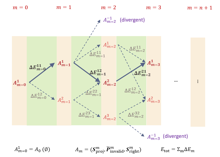
We note that some may result in , which indicates that the “preclaimed” can never be satisfied, and thus no can be found. Those branches that cannot reach are called “divergent branches”. Thus the above one-to-one correspondence is restricted to the full path so that these “divergent branches” are excluded. The automaton structure of the local states and the transition function is visualized in Fig. 1.
The last question to address before employing \threfstab_gs is the determination of from and . Different from the failed solution given in Sec. II.3.1, this question is trivial now since is directly given by , as stated in \threfSright_to_Qm. To preserve the form of Eq. (13) and (14), we can effectively define
| (22) |
With the above definitions of and , it is ready for us to derive the exact 1D local algorithm:
Theorem 2.
With the local state defined in Eq. (20) and the function defined in \threfdef:Am_to_Am+1, \threfstab_gs provides the exact algorithm to identify the stabilizer ground state of a given 1D local Hamiltonian.
Proof.
We prove that, if we exclude the “divergent branches”, satisfies the condition in Eq. (8), and consequently the stabilizer ground state of any given 1D local Hamiltonian can be obtained by applying \threfstab_gs. Furthermore, including such divergent branches is proved to not affect the final results, thus \threfstab_gs combined with itself is sufficient to give the stabilizer ground state.
We first strictly define a function , designed to filter out the divergent outcomes produced by , as:
| (23) |
Schematically can be interpreted as defined in the central region illustrated in Fig. 1. According to the previous conclusion of the one-to-one correspondence between and , we immediately conclude that satisfies the condition in Eq. (8), and thus \threfstab_gs with gives the stabilizer ground state.
Now we show that provides exactly the same result with . Let be a “convergent branch”, i.e., there exists an such that , . The only situation in which differs from is when generates a “divergent branch” , while does not. However, such an would never generate any “convergent branch” with via . Otherwise, a path could be generated by , contradicting to the assumption that is a “divergent branch”. Thus replacing by does not change the value of and defined in \threfdef:E_Am as long as is a “convergent branch”. Finally, we naturally conclude that \threfstab_gs combined with correctly gives the stabilizer ground state. ∎
We additionally comment that the automaton structure shown in Fig. 1 can potentially be applied to different tasks, such as determining excited states and performing thermal state sampling.
Finally, we estimate the computational scaling of the exact 1D local algorithm. We start by considering the number of possible generated from and . However, it does not have a simple expression due to the similar reason mentioned in Sec. II.2. A loose upper bound is provided in the following and its detailed proof is given in Appendix V.4.
Lemma 6.
local_nS Let be a -local Hamiltonian, and there exists such that for each . For any , candidate values of could be created solely from , and each generated by and must be one of these candidates.
We rewrite with some constant for simplicity and further analysis. The total computational complexity is discussed using this expression as follows. The total cost spent on each qubit is bounded by the product of (1) the number of , (2) the number of , and (3) time to compute a single from a single . Since all stabilizer state operations used in the algorithm can be realized in polynomial scaling of , the total cost with some constant .
Similar to Sec. II.2, we consider the 1D local and sparse Hamiltonians defined as follows:
Definition 10.
For a 1D -local Pauli Hamiltonian , we say that it is sparse if .
The conclusions and lead to the final computation complexity as:
Corollary 5.
local_cost The total computational cost to obtain the stabilizer ground state for a -qubit, -local and sparse Hamiltonian satisfies for some constant .
II.4 Stabilizer ground states of infinite periodic Hamiltonians
In this section, we discuss the stabilizer ground state problem of infinite periodic Hamiltonians (referred to as periodic Hamiltonians). We will show that, for any 1D periodic local Hamiltonian, the stabilizer ground state also have periodic stabilizers, but probably with a larger period. Based on the idea of the exact 1D local algorithm presented in Sec. II.3, we present an exact algorithm for 1D periodic local Hamiltonians, namely, the exact 1D periodic local algorithm, which scales with , where is the space translation period. For general periodic Hamiltonians in higher dimensions, we speculate that the stabilizer ground states should still have periodic stabilizers. With this assumption, the formalism in Sec. II.2 is extended to general periodic Hamiltonians and the equivalence between the stabilizer ground state and the restricted maximally-commuting periodic Pauli subset is also derived.
We first review the properties of the eigenstates of periodic Hamiltonians on an infinitely long 1D lattice. Let be an operator to translate a given by some fixed number of sites, and be a Hamiltonian satisfying . Bloch’s theorem [54] states that the eigenstates of can be classified by the eigenvalue of via since and can be simultaneously diagonalized. In numerical treatments, a supercell with size is usually introduced and can take discrete values for integers [55, 56].
Now we consider stabilizer states in the qubit space. Let be the operator to translate qubit to for any . A Hamiltonian is defined to be invariant under if satisfies and for any . However, the stabilizer ground state of might not be an eigenstate of , i.e., for some . An example is , where and , and thus has a period of 3. At , can be divided into independent subsystems for each , and each subsystem has degenerate stabilizer ground states with stabilizers and , respectively. At , the interaction term breaks the degeneracy, and the stabilizers of the stabilizer ground state become alternating and . This system has a period of 6 and thus does not satisfy .
periodic_stab_gs states that the stabilizer ground state of a 1D periodic local Hamiltonian can be determined by a relaxed condition for some integer , where can be interpreted as the supercell size. The proof is given in Appendix V.5.
Theorem 3.
periodic_stab_gs Any 1D periodic local Hamiltonian satisfying has at least one degenerate stabilizer ground state with for some interger , where is defined in \threflocal_nS. Let with be the stabilizer group of the corresponding stabilizer ground state. We have for any .
periodic_stab_gs proves a very loose upper bound of the supercell size , but the actual supercell size might be small (e.g. or ) for physically reasonable Hamiltonians. A linear-scaled algorithm to find the stabilizer ground state of 1D periodic local Hamiltonian thus can be derived according to \threfperiodic_stab_gs:
Corollary 6.
Let be a 1D periodic local Hamiltonian satisfying . Let be the set of possible values of generated from for integer . According to \threflocal_nS we have . Similar to \threfdef:E_Am, for arbitrary we define and by initial values and the same evolution rules from to in Eq. (13). The stabilizer ground state of and its energy in a supercell is given by
| (24) | ||||
with
| (25) |
The algorithm stated in \threfperiodic_stab_gs is referred to as the exact 1D periodic local algorithm. We then move on to discuss higher-dimensional Hamiltonians. Although it can not be theoretically derived from \threfperiodic_stab_gs that the stabilizer ground state satisfies for translation operators in each dimension, we speculate that at least some approximated (if not exact) stabilizer ground state satisfies such condition due to its similarity to the supercell treatments of exact eigenstates.
With the assumption of , we present the stabilizer ground state theory for general infinite periodic Hamiltonians. For any stabilizer with , let , we have , and thus is also a stabilizer of . We only need to consider those such that . Strictly, we define
| (26) |
Since for any , , a naïve but useful simplification of is
| (27) |
where . Finally, the stabilizer ground state is given by
| (28) |
The minimizing Eq. (28) is referred as the restricted maximally-commuting periodic Pauli subset. In practice, we only need to determine in one supercell, and in other supercells must be the same due to . For physically reasonable Hamiltonians, it might be enough to search for the minimum stabilizer ground state energy by checking the first a few .
III Results
In this section, we first perform a few benchmarks on the exact 1D local algorithm, including (1) the computational cost in Sec. III.1 and (2) comparison with numerically optimized approximated stabilizer ground states in Sec. III.2. Furthermore, we demonstrate a few potential applications for stabilizer ground states and the corresponding algorithms on (1) generation of initial states for VQE problems for better performance in Sec. III.3 and (2) simple qualitative analysis of phase transitions in Sec. III.4. Finally, in Sec. III.5, we further develop an advanced ground state ansatz called extended stabilizer ground state to understand topological phase transitions in a 2D generalized toric code model [57].
All algorithms introduced in this work are implemented in both Python and C++ in https://github.com/SUSYUSTC/stabilizer_gs. The Python code is presented for concept illustration and readability, and the C++ code is used for optimal performance with a simple parallelization.
III.1 Computational cost of the exact 1D local algorithm
The scaling of the computation time for this exact 1D local algorithm only has a loose theoretical upper bound (\threflocal_nS and \threflocal_cost) and lacks an exact analytical formula. Therefore, we implement the algorithm in C++ and numerically benchmark the computational time. All corresponding timings are collected on an 8-core i7-9700K Intel CPU.
We consider the following stochastic -nearest Heisenberg model as the example Hamiltonian:
| (29) |
with each , i.e. all these coupling coefficients independently follow the normal distribution. We also consider the case of , for comparisons. The two models are referred to as {XX,YY,ZZ} and {XX,YY}, respectively.
Following the procedure of the exact 1D local algorithm, all the possible values of with are generated sequentially by with an initial state of , where is defined in \threfdef:Am_to_Am+1. In Figure 2(a), the computational costs of generating from are plotted as a function of site for both the {XX,YY,ZZ} and {XX,YY} models with and . Except for a few sites near the boundaries, the wall-clock time spent at each site is almost a constant for both models. This verifies that the computational cost of the 1D local algorithm scales as , as proved in \threflocal_nS. Due to the smaller number of Pauli terms in the Hamiltonian, the computational cost of the {XX,YY} model is systematically lower than the {XX,YY,ZZ} model.
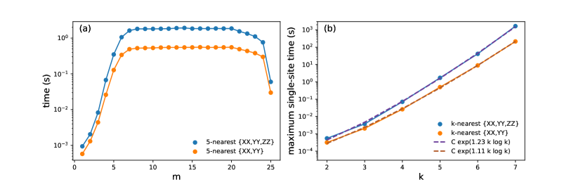
After showing that the time spent at each site is a constant except for the sites near the boundaries, we further discuss the scaling of the maximum single-site running time as a function of the locality parameter for different types of Hamiltonians. Figure 2(b) displays the maximum wall-clock time of a single site as a function of for both models. We assume that the form of the scaling function is according to \threflocal_cost. The numerical scaling functions are fitted independently for two models in Figure 2(b). The resulting fitted scaling curves have the parameters and for the {XX,YY,ZZ} and {XX,YY} models, respectively, and match the true timing data well. This indicates that the computation time of different Hamiltonians within the same class scales similarly.
III.2 Comparison with numerical discrete optimizations of stabilizer ground states
We demonstrate that numerical optimizations of stabilizer ground states are not scalable and lead to unacceptable energy errors with an increasing number of qubits. The numerical optimization of stabilizer ground states can be performed by discrete optimizations of the Clifford circuits representing stabilizer states [58].
Here, we still use the stochastic -nearest Heisenberg Hamiltonian in Eq. (29) (the {XX,YY,ZZ} model) as an example. The Clifford ansatz employed here modifies the hardware-efficient Clifford ansatz in Ref. [58] by generalizing the single-qubit Clifford rotations to all single-qubit Clifford operations (24 unique choices in total) [59]. The simulated annealing algorithm is used in the discrete optimization with an exponential decay of temperature from 5 to 0.05 in 2500 steps. In each step of the simulated annealing, one of the single-qubit Clifford operations is randomly selected and replaced with one of the 24 operations, and the move is accepted with a probability of , where is the energy difference.
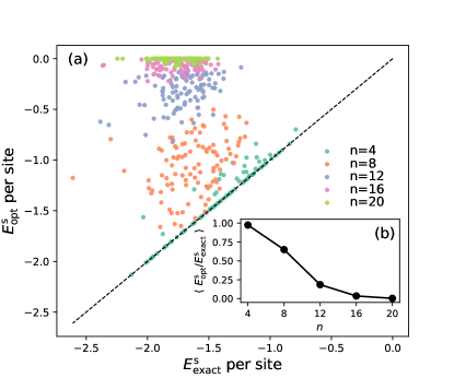
Figure 3(a) compares the stabilizer ground state energies obtained from the exact 1D local algorithm () and the numerical optimization algorithm (). For each , 100 random Hamiltonians are tested. For every single test, the numerically optimized ground state energy is either equal to or higher than the exact stabilizer ground state energy. With increasing , the success probability of the numerical optimization resulting in accurate stabilizer ground state energies decreases and approaches zero. This indicates that the numerical discrete optimization cannot correctly obtain the stabilizer ground state due to the exponential scaling of the number of stabilizer states and the number of possible Clifford circuits. Figure 3(b) displays the quantitative statistics of the performance degradation speed of numerical optimization by plotting the averaged relative stabilizer ground state energy versus the number of sites with . A rapid decay of the energy ratio is observed from 97.4% at to 0.4% at . Therefore, the optimization method fails to bootstrap large-scale variational quantum algorithms via stabilizer initializations as claimed in Ref. [58] and the challenge is fully solved by our new algorithm at least in the 1D case.
III.3 Initial state for VQE problems
Stabilizer states have been recently used as initial states [58, 60] for VQE problems to mitigate the notorious barren plateau issue [61, 62, 63]. The stabilizer initial states can be prepared on quantum circuits by efficient decomposition to up to single-qubit and double-qubit Clifford gates [25]. The effective VQE ansatz is
| (30) |
where the stabilizer initial state is decomposed to . Another approach is to employ the quantum state ansatz as follows:
| (31) |
The advantage of the latter approach is that one can equivalently transform the Hamiltonian by classically, and thus only the part needs to be performed on the quantum circuit [48, 47, 64]. However, its disadvantage is that it might break the locality of the Hamiltonian and cause additional costs on the hardware that cannot support nonlocal operations [65, 66]. Therefore, we adopt the former strategy in Eq. (30) for the following benchmark.
The {XX,YY,ZZ} model in Eq. (29) still serves as the example Hamiltonian, and the variational Hamiltonian ansatz [67] is used as the example VQE circuit for ground state optimization. By rewriting the Hamiltonian as with , the corresponding quantum circuit ansatz is as follows:
| (32) |
We compare two choices of the initial state , including the state (referred to as zero state) and the stabilizer ground state obtained by the exact 1D local algorithm. The quantum circuit simulations are conducted via the TensorCircuit software [68]. The optimization of parameters is performed by the default L-BFGS-B [69] optimizer in SciPy [70] with zero initial values.
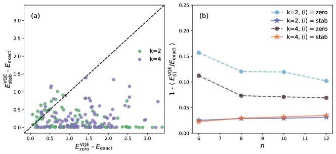
Figure 4(a) displays the distributions of optimized energy errors obtained from the two initialization strategies tested on 100 random Hamiltonians with . Stabilizer state initializations result in lower VQE errors compared with those via the zero state in 82% and 92% of the 100 tests for and , respectively. There are few points in the region of , which is attributed to the fact that an initialization state with a lower energy does not guarantee a lower final energy after VQE optimizations. Figure 4(b) also shows the mean relative errors of energies for increasing and , where (i) represents each initialization strategy. Initializations via stabilizer ground states are observed to systematically provide better energy estimations for both and .
III.4 Qualitative analysis of phase transitions
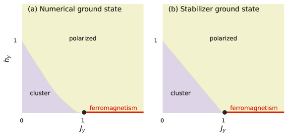
Similar to the mean-field states, stabilizer ground states can also qualitatively capture the phases and phase transitions in many interesting systems. Specifically, stabilizer ground states are good at capturing topological phases with long-range entanglements. This capability is demonstrated using an infinite 1D generalized cluster model [71] as an example, whose Hamiltonian is
| (33) |
This model is equivalent to the free fermion model at , while it is not dual to any free fermion model at due to the lack of symmetry. This Hamiltonian has been studied by numerical density matrix renormalization group (DMRG) calculations in Ref. [71], and the corresponding phase diagram is replotted in Figure 5(a). Three phases are observed in this phase diagram, including the symmetry-protected topological phase at small but positive and , the polarized phase at , , and the ferromagnetic phase at .
We apply the exact 1D periodic local algorithm to the Hamiltonian to obtain the stabilizer ground states of this model using different parameters . Calculations are performed with candidate supercell sizes , and the minimum energy is selected as the stabilizer ground state energy. All possible types of distinct stabilizer ground states are listed in Table 1, and the corresponding phase diagram is plotted in Figure 5(b). When comparing Figure 5 (a) and (b), the stabilizer ground state phase diagram matches the numerical ground state phase diagram well except for the shape of the boundary between the cluster phase and the polarized phase. The boundary predicted by stabilizer ground states is a straight line, while the numerical boundary is slightly curved. These agreements indicate that stabilizer ground states are useful to qualitatively understand of phase transitions in quantum many-body systems and provide a new perspective compared to conventional mean-field approaches. The stabilizer ground state at the tricritical point is observed to have two new degenerate stabilizer ground states besides the stabilizer ground states in other phases. These two new stabilizer ground states have stabilizers and , respectively.
| Stabilizers | Phase | |
|---|---|---|
| Cluster | ||
| , | Polarized | |
| Ferromagnetism | ||
| Tricritical point | ||
| Tricritical point |
III.5 Extended stabilizer ground states
Stabilizer ground states can be used as a platform to develop advanced numerical methods or quantum state ansatz. As an illustration, we introduce the extended stabilizer ground state and demonstrate its capability of characterizing phase transitions of a 2D generalized toric code model. We first introduce a quantum state ansatz expressed as applying single-qubit rotations on some stabilizer states, i.e.
| (34) |
where is the vector spin operator on the th qubit. We then define the extended stabilizer ground state by the state with the lowest energy among all possible combinations of and . Instead of directly finding the value of and that minimizes the energy, we can effectively transform the Hamiltonian by
| (35) |
The stabilizer ground state of the Hamiltonian is thus a function of . Since local Hamiltonians after single-site rotations remain local with the same localities , such an extended stabilizer ground state formalism increases the expressive power without significantly complicating the problem, especially when each Pauli operator only nontrivially acts on a limited number of sites.
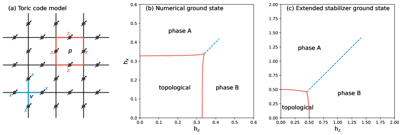
As a demonstration, we consider a 2D generalized toric code model with external magnetic fields. The Hamiltonian is
| (36) |
which is defined on a torus, where and represent the product of spin operators on bonds incident to the vertex and surrounding plaquette , respectively. The geometry of the vertices and plaquettes is shown in Figure 6(a). This Hamiltonian is studied by continuous-time Monte Carlo simulation in Ref. [72] and the phase diagram is reproduced in Figrue 6(b). At with fixed or with fixed , each spin is polarized in the or direction, and gives the phase A or B, respectively. A phase transition happens between the phase A and B at the first-order transition line , which begins at and ends at . In the limit of and , the polarization of the system varies continuously between phases A and B, thus no phase transition occurs.
Now we consider the extended stabilizer ground state of this Hamiltonian. Since the Hamiltonian only contains X and Z, the single-qubit rotations can be restricted to the form of . As stated previously, we need to transform the Hamiltonian in Eq. (36) by and then determine the stabilizer ground state. As discussed in Sec. II.4, the stabilizer ground state of a periodic local Hamiltonian should be periodic over supercells with some size . For simplification, the stabilizer ground state is assumed to have period 1. We set and for sites on vertical bonds and horizontal bonds, respectively, and thus the total rotation operator can be written as .
With fixed supercell size , the stabilizer ground state of the rotated Hamiltonian can be found via Eq. (28) for each set of rotation angles . The corresponding stabilizer ground state energy per site is written as . The extended stabilizer ground state energy per site is then given by . In the following analysis, we apply the simplification process in Eq. (27) for convenience, which allows us to exclude Pauli terms like , where the subscripts stand for the left, right, up, and down site of either a vertex or a plaquette. The valid Pauli terms of the rotated Hamiltonians include (1) and on each site; and (2) , , , and on each vertex or plaquette.
The resulting extended stabilizer ground state phase diagram is plotted in Figure 6(c) and it matches the exact phase diagram qualitatively. In the topologically ordered phase, the stabilizers are the set of all , , , on all vertices and plaquettes. We find that the corresponding is a constant with respect to and , attributed to the fact that is a symmetry operation of this stabilizer state. In phase A and B, the stabilizers are simply on each site and on each vertex and plaquette, which corresponds to the product of single-site polarized states in the picture of the unrotated Hamiltonian. We consider the first-order transition line at , in which case the extended stabilizer ground state is always found at . The corresponding per-site energy function is given by
| (37) |
which is symmetric under . No phase transition happens for large since only one minimum , while two minimums can be found for small . This is a signal of the end of the first-order transition. It is located at
| (38) |
which gives . Furthermore, at , is higher than the energy of the topologically ordered state for all . Thus, we claim that the corresponding first-order transition line begins at and ends at . Although the exact transition values are different, the qualitative picture obtained by the extended stabilizer ground state is consistent with the ground truth.
IV Conclusions and Outlook
In this work, we introduce the concept of stabilizer ground states as a versatile toolkit to qualitatively analyze quantum systems, improve quantum algorithms, and develop advanced ground state ansatzes. For general Hamiltonians, we establish the equivalence between the stabilizer ground state and the restricted maximally-commuting Pauli subset. For 1D local Hamiltonians, we additionally developed an exact and efficient algorithm that ensures a linear computational scaling with the system size to obtain the stabilizer ground state. We further extend the formalism for general Hamiltonians and the linear-scaled algorithm for 1D local Hamiltonians to infinite periodic systems. By benchmarking on example Hamiltonians, we verified the computational scaling of the exact 1D local algorithm and demonstrated the substantial performance gain over the traditional discrete optimization strategies. We also illustrate that stabilizer ground states are promising tools for various applications, including qualitative analysis of phase transitions, generating better heuristics for VQE problems, and developing more expressive ground state ansatzes.
Looking forward, future studies can fruitfully branch into three major directions.
The first avenue is to delve into algorithms for stabilizer ground states of Hamiltonians with more sophisticated structures.
A promising example would be generalizing the 1D local algorithm to other quasi-1D structures, such as structures with closed loops and tree-like lattice structures.
For local Hamiltonians in higher dimensions, finding the exact stabilizer ground state can be proved as NP-hard, evidenced by the NP-hardness of one of its simplified cases, i.e., the ground state problem of 2D classical spin models with random magnetic fields [73, 74].
Nonetheless, approximate or heuristic algorithms [75, 76] for stabilizer ground states may still be practically useful for higher dimensional systems.
The second avenue extends the concept of the stabilizer ground states to other physically interested properties, like excited states and thermal state sampling.
These extensions are plausible as the automaton structure of the 1D algorithm shares similarities with an ensemble of quantum states.
The third avenue involves the exploration of more downstream applications for stabilizer ground states.
Possible candidates include developing advanced numerical methods via perturbation theories [45] or low-rank (or low-energy) stabilizer decomposition [43].
Acknowledgement
J.S. gratefully acknowledges the support from Hongyan Scholarship.
V Appendix
V.1 Proof of \threfsparse_gs
Proof.
Let , be one of the stabililizer group such that , and is any stabilizer state stabilized by . Let , obviously we have . Let where each , . We consider the sequence with . Clearly we have , for each .
First we prove for each . Obviously it is true for . Given it is true for , we then consider . If , then so . Otherwise we consider , and . For each , it falls into one of the following situations: (1) so it contributes equally to , and , (2) but so it contributes no energy to and opposite energy to and , (3) so it contributes no energy to , and . Thus we have . However is already the minimum of for , thus , i.e. . Now we can conclude that for each , which implies .
Next, we prove is a (degenerate) stabilizer ground state. According to \threfstab_energy, we have . If there exists stabilizer state such that , we should have , which conflicts with the definition of . Thus we conclude that is a (degenerate) stabilizer ground state. ∎
V.2 Validity of for constructed by
We prove the validity of by showing that, as long as is valid for any , then is also valid.
Lemma 7.
Qm+1_valid Let be a path such that and , . It naturally defines for . If the statement that (1) is valid to add to , and (2) is true for each , then it is also true for .
Proof.
Since each is valid, we have , for . We then prove two intermediate conclusions:
First we prove from rule 2(b). In fact we have from . Since the commutation/anticommutation relations between Paulis and only depends on their values at shared sites, we must have . Thus .
Then according to rule 2(c) in \threfdef:Am_to_Am+1 we have
| (39) | ||||
where we used in the second line.
Combining the above two intermediate conclusions, we finally have
| (40) | ||||
which finishes the part (2) of the statement for . Rule 2(d) is used in the third line, and Eq. (39) is used in the fifth line. As a consequence, we also have , i.e. , which is exactly the last condition of \threfvalidQm for qubit . Combined with rule 2(a), we can conclude that is valid to add to , which finishes the part (1) of the statement. ∎
V.3 One-to-one correspondence between generated by and
In order to prove such one-to-one correspondence, we need to prove (1) each path generated from and is exactly some , and (2) each is a path generated from and .
We first prove the former one:
Lemma 8.
valid_path_to_Q For any path such that and , , there exists such that for each .
Proof.
Let with . According to \threfQm+1_valid, each is valid to add to since the statement at is trivially satisfied. Thus we automatically have and for each . We then prove . We begin with , where we have according to rule 2(b) in \threfdef:Am_to_Am+1, thus and holds at . If it holds for , according to rule 2(d) in \threfdef:Am_to_Am+1, we have
Thus holds for each . Finally we conclude that for each . ∎
To prove the latter one, it suffices to prove:
Lemma 9.
Q_to_valid_path For any , for each .
Proof.
We only need to show that the rules in \threfdef:Am_to_Am+1 are satisfied for each and . We check them one by one.
-
1.
Rule 2(a) is obvious according to \threfSright_to_Qm.
-
2.
For rule 2(b) we have
(41) -
3.
For rule 2(c), with
(42) and
(43) we have
(44) -
4.
For rule 2(d) we have
(45)
∎
Combining the \threfvalid_path_to_Q and \threfQ_to_valid_path, we have proved the one-to-one correpondence between generated by and .
V.4 Proof of \threflocal_nS
Proof.
According to \threfQm+1_valid, for each (partial) path , let , we always have , and , even if some elements in are “divergent branches”. In the following, we give the upper bound of the number of pairs and the number of separately.
First, we prove that the pair can be determined from
| (46) |
For we have
| (47) | ||||
For , since has , any with must have and thus , so we have . Thus
| (48) | ||||
According to the definition in Eq. (46) we now conclude
| (49) |
Since any with must have , has at most non-identity elements. Also is a qubit stabilizer group. According to \threfnS, there are at most choices of .
Finally, we have
| (50) |
For a similar reason, there are at most non-identity elements in . Thus there are at most choices of .
Combining the above two upper bounds, there are at most different candidates values of . Also both and can be determined by . Thus the candidates of can be determined by . ∎
V.5 Proof of \threfperiodic_stab_gs
Proof.
We first consider the Hamiltonian on a finite chain with sites. We denote the Hamiltonian with sites as . According to the exact 1D local algorithm, we can start from at the beginning and generate by . Following the proof of \threflocal_nS, there are at most candidate values of . These candidate values of are fully determined by the surrounding environment which is again periodic, i.e. . Thus for those differ by multiples of , they have the same (and finite) candidate values of . Thus there must exist with .
Now we prove that the stabilizer ground state energy per site of the infinite Hamiltonian is
| (51) |
where is defined in \threfdef:E_Am. If there exists an infinite stabilizer state with a lower per-site energy than , then for sufficiently large , the stabilizer ground state energy of the finite Hamiltonian can be lower than by arbitrary amount of energy , i.e. . Let the stabilizer group of the corresponding stabilizer state be , , and let for each . If , we can find such that . Then we have according to the definition of . Now we remove from the path , and consider the new path , where . In fact, it still satisfies for each , thus it exactly maps to the stabilizer ground state of with energy . We can then continue the above deleting process and create , , …, until we end up with some and the corresponding path . Such a path can map to some -qubit stabilizer state with energy . However should have a finite lower bound in the order of , which is independent of . Thus cannot be arbitrarily large, which conflicts with the assumption. Thus we conclude that is the stabilizer ground state energy per site.
Let , and minimize Eq. (51). Let be one of the path satisfies . We can construct a stabilizer state with the stabilizer group with for each , where satisfies (mod ), where is the supercell size. According to \threfstab_gs, this state gives exactly the per-site energy , thus it is (one of) the stabilizer ground state of the infinite periodic Hamiltonian . The corresponding path thus satisfies for any . ∎
References
- Kitaev et al. [2002] A. Kitaev, A. H. Shen, and M. N. Vyalyi, Classical and Quantum Computation, 47 (American Mathematical Soc., Providence, 2002).
- Aharonov and Naveh [2002] D. Aharonov and T. Naveh, Quantum NP - A Survey, arXiv:quant-ph/0210077 (2002), arXiv:quant-ph/0210077 .
- Kempe et al. [2006] J. Kempe, A. Kitaev, and O. Regev, The complexity of the local Hamiltonian problem, SIAM J. Comput. 35, 1070 (2006).
- Schuch and Verstraete [2009] N. Schuch and F. Verstraete, Computational complexity of interacting electrons and fundamental limitations of density functional theory, Nat. Phys. 5, 732 (2009).
- Huang [2021] Y. Huang, Two-dimensional local Hamiltonian problem with area laws is QMA-complete, J. Comput. Phys. 443, 110534 (2021).
- Lee et al. [2023] S. Lee, J. Lee, H. Zhai, Y. Tong, A. M. Dalzell, A. Kumar, P. Helms, J. Gray, Z.-H. Cui, W. Liu, et al., Evaluating the evidence for exponential quantum advantage in ground-state quantum chemistry, Nat. Commun. 14, 1952 (2023).
- Verstraete et al. [2008] F. Verstraete, V. Murg, and J. Cirac, Matrix product states, projected entangled pair states, and variational renormalization group methods for quantum spin systems, Adv. Phys. 57, 143 (2008).
- Schollwöck [2011] U. Schollwöck, The density-matrix renormalization group in the age of matrix product states, Ann. Phys. 326, 96 (2011).
- Liao et al. [2019] H.-J. Liao, J.-G. Liu, L. Wang, and T. Xiang, Differentiable programming tensor networks, Phys. Rev. X 9, 31041 (2019).
- Carleo and Troyer [2017] G. Carleo and M. Troyer, Solving the quantum many-body problem with artificial neural networks, Science 355, 602 (2017).
- Deng et al. [2017] D.-L. Deng, X. Li, and S. Das Sarma, Quantum entanglement in neural network states, Phys. Rev. X 7, 021021 (2017).
- Glasser et al. [2018] I. Glasser, N. Pancotti, M. August, I. D. Rodriguez, and J. I. Cirac, Neural-network quantum states, string-bond states, and chiral topological states, Phys. Rev. X 8, 11006 (2018).
- Chen et al. [2018] J. Chen, S. Cheng, H. Xie, L. Wang, and T. Xiang, Equivalence of restricted Boltzmann machines and tensor network states, Phys. Rev. B 97, 085104 (2018).
- Zhang et al. [2023a] S.-X. Zhang, Z.-Q. Wan, and H. Yao, Automatic differentiable Monte Carlo: Theory and application, Phys. Rev. Res. 5, 033041 (2023a).
- Sun et al. [2022] X.-Q. Sun, T. Nebabu, X. Han, M. O. Flynn, and X.-L. Qi, Entanglement features of random neural network quantum states, Phys. Rev. B 106, 115138 (2022).
- Shankar [2012] R. Shankar, Principles of quantum mechanics (Springer Science & Business Media, 2012).
- Møller and Plesset [1934] C. Møller and M. S. Plesset, Note on an approximation treatment for many-electron systems, Phys. Rev. 46, 618 (1934).
- Shavitt and Bartlett [2009] I. Shavitt and R. J. Bartlett, Many-body methods in chemistry and physics: MBPT and coupled-cluster theory (Cambridge university press, 2009).
- Bartlett and Musiał [2007] R. J. Bartlett and M. Musiał, Coupled-cluster theory in quantum chemistry, Rev. Mod. Phys. 79, 291 (2007).
- Levine et al. [2009] I. N. Levine, D. H. Busch, and H. Shull, Quantum chemistry, Vol. 6 (Pearson Prentice Hall Upper Saddle River, NJ, 2009).
- Szabo and Ostlund [2012] A. Szabo and N. S. Ostlund, Modern quantum chemistry: Introduction to advanced electronic structure theory (Courier Corporation, 2012).
- Nielsen and Chuang [2001] M. A. Nielsen and I. L. Chuang, Quantum computation and quantum information, Phys. Today 54, 60 (2001).
- Gottesman [1998a] D. Gottesman, Theory of fault-tolerant quantum computation, Phys. Rev. A 57, 127 (1998a).
- Gottesman [1998b] D. Gottesman, The Heisenberg representation of quantum computers, arXiv preprint quant-ph/9807006 (1998b).
- Aaronson and Gottesman [2004] S. Aaronson and D. Gottesman, Improved simulation of stabilizer circuits, Phys. Rev. A 70, 052328 (2004).
- Jordan and Wigner [1993] P. Jordan and E. P. Wigner, Über das paulische äquivalenzverbot (Springer, 1993).
- Bravyi and Kitaev [2002] S. B. Bravyi and A. Y. Kitaev, Fermionic quantum computation, Ann. Phys. 298, 210 (2002).
- Macridin et al. [2018] A. Macridin, P. Spentzouris, J. Amundson, and R. Harnik, Electron-phonon systems on a universal quantum computer, Phys. Rev. Lett. 121, 110504 (2018).
- Miessen et al. [2021] A. Miessen, P. J. Ollitrault, and I. Tavernelli, Quantum algorithms for quantum dynamics: A performance study on the spin-boson model, Phys. Rev. Res. 3, 043212 (2021).
- Di Matteo et al. [2021] O. Di Matteo, A. McCoy, P. Gysbers, T. Miyagi, R. M. Woloshyn, and P. Navrátil, Improving Hamiltonian encodings with the Gray code, Phys. Rev. A 103, 042405 (2021).
- Li et al. [2023] W. Li, J. Ren, S. Huai, T. Cai, Z. Shuai, and S. Zhang, Efficient quantum simulation of electron-phonon systems by variational basis state encoder, Phys. Rev. Res. 5, 023046 (2023).
- Zeng et al. [2019] B. Zeng, X. Chen, D.-L. Zhou, and X.-G. Wen, Quantum Information Meets Quantum Matter, Quantum Science and Technology (Springer New York, New York, NY, 2019).
- Perez-Garcia et al. [2006] D. Perez-Garcia, F. Verstraete, M. M. Wolf, and J. I. Cirac, Matrix product state representations, arXiv preprint quant-ph/0608197 (2006).
- Fattal et al. [2004] D. Fattal, T. S. Cubitt, Y. Yamamoto, S. Bravyi, and I. L. Chuang, Entanglement in the stabilizer formalism, arXiv preprint quant-ph/0406168 (2004).
- Webb [2016] Z. Webb, The Clifford group forms a unitary 3-design, Quantum Info. Comput. 16, 1379–1400 (2016).
- Huang et al. [2020] H. Y. Huang, R. Kueng, and J. Preskill, Predicting many properties of a quantum system from very few measurements, Nat. Phys. 16, 1050 (2020).
- Nahum et al. [2017] A. Nahum, J. Ruhman, S. Vijay, and J. Haah, Quantum entanglement growth under random unitary dynamics, Phys. Rev. X 7, 031016 (2017).
- von Keyserlingk et al. [2018] C. W. von Keyserlingk, T. Rakovszky, F. Pollmann, and S. L. Sondhi, Operator hydrodynamics, OTOCs, and entanglement growth in systems without conservation laws, Phys. Rev. X 8, 021013 (2018).
- Nahum et al. [2018] A. Nahum, S. Vijay, and J. Haah, Operator spreading in random unitary circuits, Phys. Rev. X 8, 021014 (2018).
- Gottesman [1997] D. Gottesman, Stabilizer codes and quantum error correction, arXiv preprint quant-ph/9705052 (1997).
- Fowler et al. [2012] A. G. Fowler, M. Mariantoni, J. M. Martinis, and A. N. Cleland, Surface codes: Towards practical large-scale quantum computation, Phys. Rev. A 86, 032324 (2012).
- Nayak et al. [2008] C. Nayak, S. H. Simon, A. Stern, M. Freedman, and S. Das Sarma, Non-Abelian anyons and topological quantum computation, Rev. Mod. Phys. 80, 1083 (2008).
- Bravyi et al. [2019] S. Bravyi, D. Browne, P. Calpin, E. Campbell, D. Gosset, and M. Howard, Simulation of quantum circuits by low-rank stabilizer decompositions, Quantum 3, 181 (2019).
- Bravyi and Gosset [2016] S. Bravyi and D. Gosset, Improved classical simulation of quantum circuits dominated by Clifford gates, Phys. Rev. Lett. 116, 250501 (2016).
- Begušić et al. [2023] T. Begušić, K. Hejazi, and G. K. Chan, Simulating quantum circuit expectation values by clifford perturbation theory, arXiv preprint arXiv:2306.04797 (2023).
- Cheng et al. [2022] M. Cheng, K. Khosla, C. Self, M. Lin, B. Li, A. Medina, and M. Kim, Clifford circuit initialisation for variational quantum algorithms, arXiv preprint arXiv:2207.01539 (2022).
- Zhang et al. [2023b] S. Zhang, Z.-Q. Wan, C.-Y. Hsieh, H. Yao, and S. Zhang, Variational quantum‐neural hybrid error mitigation, Adv. Quantum Technol. 6 (2023b).
- Sun et al. [2024] J. Sun, L. Cheng, and W. Li, Toward chemical accuracy with shallow quantum circuits: A Clifford-based Hamiltonian engineering approach, J. Chem. Theory Comput. 20, 695 (2024).
- Mishmash et al. [2023] R. V. Mishmash, T. P. Gujarati, M. Motta, H. Zhai, G. K.-L. Chan, and A. Mezzacapo, Hierarchical Clifford transformations to reduce entanglement in quantum chemistry wave functions, J. Chem. Theory Comput. (2023).
- Schleich et al. [2023] P. Schleich, J. Boen, L. Cincio, A. Anand, J. S. Kottmann, S. Tretiak, P. A. Dub, and A. Aspuru-Guzik, Partitioning quantum chemistry simulations with clifford circuits, arXiv preprint arXiv:2303.01221 (2023).
- Gross [2006] D. Gross, Hudson’s theorem for finite-dimensional quantum systems, J. Math. Phys. 47 (2006).
- Hopcroft et al. [2001] J. E. Hopcroft, R. Motwani, and J. D. Ullman, Introduction to automata theory, languages, and computation, Acm Sigact News 32, 60 (2001).
- Salomaa [2014] A. Salomaa, Theory of automata (Elsevier, 2014).
- Bloch [1929] F. Bloch, Über die quantenmechanik der elektronen in kristallgittern, Zeitschrift für physik 52, 555 (1929).
- Kratzer and Neugebauer [2019] P. Kratzer and J. Neugebauer, The basics of electronic structure theory for periodic systems, Front. Chem. 7, 106 (2019).
- Martin [2020] R. M. Martin, Electronic structure: basic theory and practical methods (Cambridge university press, 2020).
- Kitaev [2003] A. Y. Kitaev, Fault-tolerant quantum computation by anyons, Ann. Phys. 303, 2 (2003).
- Ravi et al. [2022] G. S. Ravi, P. Gokhale, Y. Ding, W. Kirby, K. Smith, J. M. Baker, P. J. Love, H. Hoffmann, K. R. Brown, and F. T. Chong, Cafqa: A classical simulation bootstrap for variational quantum algorithms, in Proceedings of the 28th ACM International Conference on Architectural Support for Programming Languages and Operating Systems, Volume 1 (2022) pp. 15–29.
- Koenig and Smolin [2014] R. Koenig and J. A. Smolin, How to efficiently select an arbitrary Clifford group element, J. Math. Phys. 55 (2014).
- Bhattacharyya and Ravi [2023] B. Bhattacharyya and G. S. Ravi, Optimal Clifford initial states for Ising Hamiltonians, in 2023 IEEE International Conference on Rebooting Computing (ICRC) (IEEE, 2023) pp. 1–10.
- Cerezo et al. [2021] M. Cerezo, A. Sone, T. Volkoff, L. Cincio, and P. J. Coles, Cost function dependent barren plateaus in shallow parametrized quantum circuits, Nat. Commun. 12, 1791 (2021).
- McClean et al. [2018] J. R. McClean, S. Boixo, V. N. Smelyanskiy, R. Babbush, and H. Neven, Barren plateaus in quantum neural network training landscapes, Nat. Commun. 9, 4812 (2018).
- Zhang et al. [2023c] H.-K. Zhang, S. Liu, and S.-X. Zhang, Absence of barren plateaus in finite local-depth circuits with long-range entanglement, arXiv:2311.01393 (2023c).
- Shang et al. [2023] Z.-X. Shang, M.-C. Chen, X. Yuan, C.-Y. Lu, and J.-W. Pan, Schrödinger-Heisenberg variational quantum algorithms, Phys. Rev. Lett. 131, 060406 (2023).
- Kim et al. [2023] Y. Kim, A. Eddins, S. Anand, K. X. Wei, E. Van Den Berg, S. Rosenblatt, H. Nayfeh, Y. Wu, M. Zaletel, K. Temme, et al., Evidence for the utility of quantum computing before fault tolerance, Nature 618, 500 (2023).
- Arute et al. [2019] F. Arute, K. Arya, R. Babbush, D. Bacon, J. C. Bardin, R. Barends, R. Biswas, S. Boixo, F. G. Brandao, D. A. Buell, et al., Quantum supremacy using a programmable superconducting processor, Nature 574, 505 (2019).
- Wiersema et al. [2020] R. Wiersema, C. Zhou, Y. de Sereville, J. F. Carrasquilla, Y. B. Kim, and H. Yuen, Exploring entanglement and optimization within the Hamiltonian variational ansatz, PRX Quantum 1, 020319 (2020).
- Zhang et al. [2023d] S.-X. Zhang, J. Allcock, Z.-Q. Wan, S. Liu, J. Sun, H. Yu, X.-H. Yang, J. Qiu, Z. Ye, Y.-Q. Chen, C.-K. Lee, Y.-C. Zheng, S.-K. Jian, H. Yao, C.-Y. Hsieh, and S. Zhang, Tensorcircuit: A quantum software framework for the NISQ era, Quantum 7, 912 (2023d).
- Byrd et al. [1995] R. H. Byrd, P. Lu, J. Nocedal, and C. Zhu, A limited memory algorithm for bound constrained optimization, SIAM J. Sci. Comput. 16, 1190 (1995).
- Virtanen et al. [2020] P. Virtanen, R. Gommers, T. E. Oliphant, M. Haberland, T. Reddy, D. Cournapeau, E. Burovski, P. Peterson, W. Weckesser, J. Bright, S. J. van der Walt, M. Brett, J. Wilson, K. J. Millman, N. Mayorov, A. R. J. Nelson, E. Jones, R. Kern, E. Larson, C. J. Carey, İ. Polat, Y. Feng, E. W. Moore, J. VanderPlas, D. Laxalde, J. Perktold, R. Cimrman, I. Henriksen, E. A. Quintero, C. R. Harris, A. M. Archibald, A. H. Ribeiro, F. Pedregosa, P. van Mulbregt, and SciPy 1.0 Contributors, SciPy 1.0: Fundamental algorithms for scientific computing in Python, Nat. Methods 17, 261 (2020).
- Verresen et al. [2017] R. Verresen, R. Moessner, and F. Pollmann, One-dimensional symmetry protected topological phases and their transitions, Phys. Rev. B 96, 165124 (2017).
- Wu et al. [2012] F. Wu, Y. Deng, and N. Prokof’ev, Phase diagram of the toric code model in a parallel magnetic field, Phys. Rev. B 85, 195104 (2012).
- Barahona [1982] F. Barahona, On the computational complexity of Ising spin glass models, J. Phys. A Math. Gen. 15, 3241 (1982).
- Zhang [2019] S.-X. Zhang, Classification on the computational complexity of spin models, arXiv preprint arXiv:1911.04122 (2019).
- Zhang et al. [2022] S.-X. Zhang, C.-Y. Hsieh, S. Zhang, and H. Yao, Differentiable quantum architecture search, Quantum Sci. Technol. 7, 045023 (2022).
- Gu et al. [2023] A. Gu, H.-Y. Hu, D. Luo, T. L. Patti, N. C. Rubin, and S. F. Yelin, Zero and finite temperature quantum simulations powered by quantum magic, arXiv preprint arXiv:2308.11616 (2023).