Modelling of initially stressed solids: structure of the energy density in the incompressible limit

Abstract

This study addresses the modelling of elastic bodies, particularly when the relaxed configuration is unknown or non-existent. We adopt the theory of initially stressed materials, incorporating the deformation gradient and stress state of the reference configuration (initial stress tensor) into the response function. We show that for the theory to be applicable, the response function of the relaxed material is invertible up to an element of the material symmetry group. Additionally, we establish that commonly imposed constitutive restrictions, namely the initial stress compatibility condition and initial stress reference independence, naturally arise when assuming an initial stress generated solely from elastic distortion. The paper delves into modelling aspects concerning incompressible materials, showcasing the expressibility of strain energy density as a function of the deviatoric part of the initial stress tensor and the isochoric part of the deformation gradient. This not only reduces the number of independent invariants in the energy functional, but also enhances numerical robustness in finite element simulations. The findings of this research hold significant implications for modelling materials with initial stress, extending potential applications to areas such as mechanobiology, soft robotics, and 4D printing.

1 Introduction

In the modelling of solid materials, the elastic strain is typically defined with respect to a chosen configuration known as the reference configuration. While it is commonly selected as a configuration free of mechanical stress, certain situations necessitate adopting a reference configuration that exhibits a non-zero stress state. The stress distribution in this reference configuration is called initial stress.

This circumstance is particularly prevalent in biological tissues, which are frequently subject to external mechanical force (e.g. the blood pressure on vessel walls and on the heart chambers) and their stress free configuration is not easily observable [3]. An initial stress generated by the imposition of external loads is also known as pre-stress [41]. Pre-stress magnitude and distribution can be designed to enhance the mechanical response of materials, as seen in pre-stressed concrete structures [33].

Moreover, materials may store mechanical stress even in the absence of external forces. In such a case the stress state is referred to as residual stress [18]. In general, residual stresses are generated by geometrical incompatibilities at the microstructural level that necessitate the introduction of elastic distortions to maintain the continuity of the body [13]. To provide some examples, the formation of residual stress in biological materials is driven by active processes, e.g. growth, that generate the incompatibility [46, 6]. Residual stresses may also arise in engineering materials as well, in this case as a result of their manufacturing process [49, 51, 31, 36, 8].

Regardless of its origin, a suitable design of the initial stress distribution can be exploited to enhance the resistance of the material to the deformation, e.g. in arteries [5, 26], or to control the shape morphing of the object [7, 43], with possible applications to soft robotics [1] and 4D printing [47, 52].

A successful approach to modelling initially stressed material is based on the introduction of a virtual relaxed state of the body [44]. The underlying idea is based on a multiplicative decomposition of the deformation gradient $\mathsf{F}=\mathsf{F}_{\text{e}}\mathsf{G}$, where $\mathsf{G}$ maps the reference configuration to a relaxed state while $\mathsf{F}_{\text{e}}$ accounts for the local elastic distortion. In general, $\mathsf{G}$ may not be the gradient of a deformation. This introduces incompatibilities that generate the initial stress within the body. Despite the huge success of this theory, the main drawback is that $\mathsf{G}$ must be constitutively provided. Experimental measurements of $\mathsf{G}$ usually rely on cutting the body to release the mechanical stress and reveal its relaxed state. Clearly, such a destructive technique is not applicable in several scenarios, such as the in-vivo estimation of the stress state of a biological tissue.

However, recent scientific developments have made it possible to measure the initial stress state of an object using non destructive methods, such as acoustoelastic techniques [32, 50]. Based on these progresses, it is more effective to describe the material behaviour as a function of the initial stress tensor and of the deformation gradient. Such an approach is known as the theory of initially stressed materials. The first attempts in this direction date back to the seminal works of Hoger and colleagues [19, 21, 22, 20, 28, 29, 30]. Further extensions have been proposed in recent years [45, 35, 23, 37, 10, 27]. Specifically, Shams et al. [45] proposed a constitutive law for a hyperelastic and isotropic solid based on ten invariants involving the elastic deformation and the initial stress tensor.

More recently, several constitutive restrictions have been proposed to guide the construction of physically admissible energy functions, such as the initial stress compatibility and the initial stress reference independence conditions [14, 15]. Despite these advances, a unified theory for constitutive modelling of initially stressed solids remains a debated topic [40] and it is still not clear which constitutive laws are admissible. Furthermore, the finite element simulations of incompressible initially stressed solids exhibit numerical issues, as highlighted for example in [7]. These problems are related to locking phenomena that frequently affect the simulation of incompressible elastic media (see chapter 15 of [9]). A common approach to circumvent these drawbacks in conventional hyperelasticity is to exploit a decomposition of the stress tensors into a volumetric and a deviatoric part [4, 25].

Based on the aforementioned aspects, the purpose of this paper is two-fold:

• derive a comprehensive theory of initially stressed materials where the initial stress is generated solely by an elastic distortion,

• enhance current description of incompressible initially stressed media exploiting the volumetric-deviatoric splitting.

The paper is organised as follows: in Section 2, we review the basic theory of initially stressed materials, deriving it starting by solely assuming that the initial stress is generated by an elastic distortion. Specifically, we show that commonly enforced restrictions naturally follow from this assumption. In Section 3, we provide a representation formula for the strain energy density of an isotropic initially stressed material. In Section 4 we study the incompressible limit of the proposed theoretical framework. As an application, the bending of an initially stressed block is analysed in Section 5.

2 Initially stressed materials

In the following, we introduce the essential notation and theory to describe the response of initially-stressed materials by exploiting the theoretical framework developed by Shams et al. [45].

We consider a reference configuration $\Omega_{0}\subset\mathbb{E}^{3}$, with $\boldsymbol{\mathbf{X}}\in\Omega_{0}$ representing a material position vector. The deformation field is denoted by the map $\boldsymbol{\mathbf{\chi}}:\Omega_{0}\rightarrow\mathbb{E}^{3}$, where $\boldsymbol{\mathbf{x}}=\boldsymbol{\mathbf{\chi}}(\boldsymbol{\mathbf{X}})$ is the current position vector. The deformation gradient tensor yields $\mathsf{F}=\operatorname{Grad}\boldsymbol{\mathbf{\chi}}$.

Let $\mathsf{T}$ and $\psi$ be the Cauchy stress tensor and the strain energy density per unit reference volume, respectively. We recall that the first Piola-Kirchhoff stress tensors $\mathsf{S}$ is related to $\mathsf{T}$ by the formula

$$\mathsf{T}=J^{-1}\mathsf{S}\mathsf{F}^{T},$$ (1)

where $J=\det\mathsf{F}$.

When modelling initially stressed materials, it is usually assumed that both the strain energy density and the Cauchy stress tensor depend on the initial stress tensor $\mathsf{\Upsigma}$ and the deformation gradient, that is

$$\psi=\widehat{\psi}(\mathsf{F},\,\mathsf{\Upsigma})\quad\text{and}\quad\mathsf{T}=\widehat{\mathsf{T}}(\mathsf{F},\,\mathsf{\Upsigma}).$$ (2)

Before proceeding into this direction, we present a simple one-dimensional example to illustrate the procedure.

2.1 A 0D illustrative example: an initially stressed elastic spring

We consider an elastic spring in its relaxed state. In this configuration, its length $L$ coincides with its rest length. We can write its constitutive response out of this stress free state as simply as

$$F=f(\lambda)\,,$$ (3)

where $F$ is the elastic force generated by the spring, $\lambda=\ell/L$ is the stretch, and $\ell$ is the current length of the spring (see Fig. 1). We further assume $f$ to be invertible and specifically take a linear function $f(\lambda)=-kL(\lambda-1)$, where $k$ is the elastic constant.

We now consider a different configuration of the spring with length $L_{1}\neq L$. According to (3), an elastic force $\tau_{1}=f(e_{1})$, with $e_{1}=L_{1}/L$, is associated with this configuration. Our aim is to describe the response of the spring out of this stressed configuration. Accordingly, we shall introduce a constitutive function $f_{1}$ that depends exclusively on the stretch $\lambda_{1}=\ell/L_{1}$ and on the force $\tau_{1}$. Since $\lambda=e_{1}\lambda_{1}=f^{-1}(\tau_{1})\lambda_{1}$, we have

$$F=f_{1}(\lambda_{1},\,\tau_{1})=f(f^{-1}(\tau_{1})\lambda_{1}).$$ (4)

Similarly, we can take another configuration with length $L_{2}\neq L_{1}$. By following the same procedure used above, we can build a constitutive function $f_{2}$ out of this configuration as follows

$$F=f_{2}(\lambda_{2},\,\tau_{2})=f(f^{-1}(\tau_{2})\lambda_{2}).$$ (5)

where $\tau_{2}=f(e_{2})$, with $e_{2}=L_{2}/L$, and the stretch $\lambda_{2}=\ell/L_{2}$.

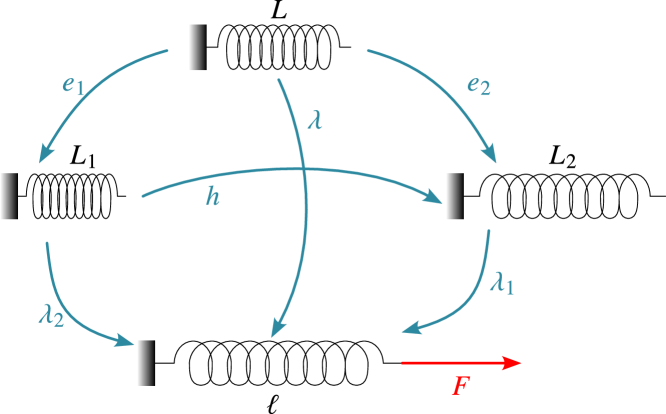
Figure 1: A scheme of the example of section 2.1.

At this point, we observe that $f_{1}$ and $f_{2}$ defined in (4) and (5) are merely the same response function that is evaluated for different values. To support this, we introduce $h=L_{2}/L_{1}=\lambda_{1}\lambda_{2}^{-1}$, so it can be easily shown that

$$F=f_{1}(\lambda_{2}h,\tau_{1})=f_{2}(\lambda_{2},\,\tau_{2})=f_{1}(\lambda_{2},\,\tau_{2})\,.$$

Moreover, since $\tau_{2}=f_{1}(h,\,\tau_{1})$, we get

$$f_{1}(\lambda_{2}h,\tau_{1})=f_{1}(\lambda_{2},\,f_{1}(h,\,\tau_{1}))\,.$$ (6)

This last equation is the one-dimensional equivalent of the initial stress reference independence condition proposed in [15] for initially-stressed materials. A key element in this derivation is the assumption of a common relaxed state of the initially stressed spring. Although such an example is an over-simplification of a generic multidimensional problem, it enlightens two key assumptions

1. The invertibility of the response function $f$.

2. The fact that the initial stress state is generated by an elastic distortion.

We now extend this considerations to a three-dimensional elastic body with initial stress to study the general structure of the problem.

2.2 Initially-stressed three-dimensional elastic bodies: fundamental assumptions

We consider an hyperelastic material such that the process of formation of the mechanical stress is purely elastic. The following notation will be used thereafter

• $\operatorname{Lin}$ denotes the set of linear second order tensors.

• $\operatorname{Lin}^{+}$ denotes the set of all the $\mathsf{F}\in\operatorname{Lin}$ such that $\det\mathsf{F}>0$.

• $\operatorname{Sym}$ is the set of all the symmetric second order tensors.

• $\operatorname{Orth}$ and $\operatorname{Orth}^{+}$ are the sets of the orthogonal matrices and of rotations, respectively.

2.2.1 Invertibility of the response function

As pursued in Sec. 2.1, we start from the well-known theory of hyperelastic materials free of initial stresses. By denoting with $\Omega_{0}$ a given relaxed reference configuration, the constitutive law takes the usual form $\mathsf{T}_{0}(\mathsf{F}_{\text{e}})$, where $\mathsf{F}_{\text{e}}\in\operatorname{Lin}^{+}$ is an elastic distortion from $\Omega_{0}$ to the current state of the material (see Fig. 2). The strain energy density associated with $\mathsf{T}_{0}(\mathsf{F}_{\text{e}})$ is $\psi_{0}(\mathsf{F}_{\text{e}})$.

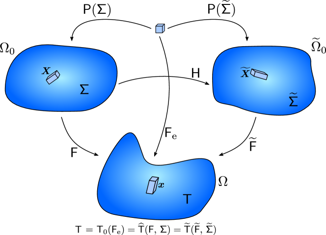
Figure 2: Change of reference configuration for initially stressed materials.

For each stress state $\mathsf{\Upsigma}\in\operatorname{Sym}$, we would like to identify an elastic distortion $\mathsf{P}_{\mathsf{\Upsigma}}$ such that $\mathsf{T}_{0}(\mathsf{P}_{\mathsf{\Upsigma}})=\mathsf{\Upsigma}$. The existence of such a distortion $\mathsf{P}_{\mathsf{\Upsigma}}$ has been addressed in [42] provided that the strain energy density is non degenerate, that is

$$\left\{\begin{aligned} &\psi_{0}(\mathsf{F}_{\text{e}})\rightarrow+\infty\qquad\text{as }|\mathsf{F}_{\text{e}}|+|\mathsf{F}_{\text{e}}^{-1}|+\det\mathsf{F}_{\text{e}}\rightarrow+\infty,\\ &\psi_{0}(\mathsf{F}_{\text{e}})\rightarrow+\infty\qquad\text{as }\det\mathsf{F}_{\text{e}}\rightarrow 0.\end{aligned}\right.$$

Such an assumption requires the strain energy density to blow up when the body is locally subject to an extreme deformation (e.g. one of the principal stretches goes to infinity). However, the simple existence of $\mathsf{P}_{\mathsf{\Upsigma}}$ is not enough, as we show next.

Compared with the 0D example, we cannot have an exact inverse of $\mathsf{T}_{0}$ in this 3D case. Indeed, for any $\mathsf{Q}\in\mathcal{G}$, where $\mathcal{G}\subset\operatorname{Orth}^{+}$ is the material symmetry group, we have

$$\mathsf{T}_{0}(\mathsf{F}_{\text{e}}\mathsf{Q})=\mathsf{T}_{0}(\mathsf{F}_{\text{e}})\,,$$

so that $\mathsf{T}_{0}$ is not injective, in general. Nevertheless, it is possible to introduce a relation of equivalence $\sim$ in $\operatorname{Lin}^{+}$, such that

$$\mathsf{F}_{\text{e}}^{(1)}\sim\mathsf{F}_{\text{e}}^{(1)}\quad\Leftrightarrow\quad\exists\mathsf{Q}\in\mathcal{G}\;|\;\mathsf{F}_{\text{e}}^{(1)}=\mathsf{F}_{\text{e}}^{(2)}\mathsf{Q}\,.$$

We further define the quotient set $\mathcal{F}=\operatorname{Lin}^{+}/\sim$ composed of the equivalence classes $[\mathsf{F}_{\text{e}}]=\{\mathsf{A}\in\operatorname{Lin}^{+}\;|\;\mathsf{A}\sim\mathsf{F}_{\text{e}}\}$ induced by $\sim$, namely

$$\mathcal{F}=\{[\mathsf{F}_{\text{e}}],\,\mathsf{F}_{\text{e}}\in\operatorname{Lin}^{+}\}\,.$$

We can now conveniently construct an alternative response function $\mathsf{T}_{\mathcal{F}}$, as follows

$$\mathsf{T}_{\mathcal{F}}:\mathcal{F}\rightarrow\operatorname{Sym},$$

$$\mathsf{T}_{\mathcal{F}}([\mathsf{F}_{\text{e}}]):=\mathsf{T}_{0}(\mathsf{F}_{\text{e}}),$$

which is, of course, well defined since $\mathsf{T}_{0}(\mathsf{A})$ is independent on the choice of $\mathsf{A}\in[\mathsf{F}_{\text{e}}]$. Differently form $\mathsf{T}_{0}$, the newly introduced response function $\mathsf{T}_{\mathcal{F}}$ can be bijective under particular circumstances.

Remark 2.1.

Requiring the invertibility of the response function over the set $\mathcal{F}$ is very restrictive. Consider, for instance, an incompressible material whose strain energy density is given by

$$\psi_{0}(\mathsf{F}_{\text{e}})=\mu(\sqrt{\lambda_{1}}+\sqrt{\lambda_{2}}+\sqrt{\lambda_{3}}-3),$$

Such an energy is representative of material softening and, therefore, does not lead to an injective expression of the principal stresses. We show this fact by taking a uniaxial deformation in plane strain conditions, such that $\mathsf{F}_{\text{e}}=\operatorname{diag}(\lambda,\,\lambda^{-1},\,1)$. The principal stress along the axial direction can be computed as $t_{1}(\lambda)=\partial\psi_{0}(\mathsf{F}_{\text{e}})/\partial\lambda$, resulting in

$$t_{1}(\lambda)=\mu\frac{(\lambda-1)}{2\lambda^{3/2}},$$

which is clearly not bijective. This behaviour is linked with the existence of multiple deformations associated with the same stress response, but having different strain energy. For instance, we have

$$t_{1}\left(2\right)=t_{1}\left(3+\sqrt{5}\right),$$

but

$$\left.\psi_{0}(\mathsf{F}_{\text{e}})\right|_{\lambda=2}=\frac{3\sqrt{2}}{2}\mu<3\frac{\sqrt{10}+\sqrt{2}}{2}\mu=\left.\psi_{0}(\mathsf{F}_{\text{e}})\right|_{\lambda=3+\sqrt{5}}.$$

In order to construct a robust theory, in the following we require $\mathsf{T}_{\mathcal{F}}$ to be bijective.

This discussion simplifies a lot if we assume an isotropic material response, that is $\mathcal{G}=\operatorname{Orth}^{+}$. Accordingly, using the polar decomposition theorem $\mathsf{F}_{\text{e}}=\mathsf{V}\mathsf{R}$, with $\mathsf{V}$ being a symmetric positive definite tensor and $\mathsf{R}\in\operatorname{Orth}^{+}$, we have

$$\mathsf{T}_{0}(\mathsf{F}_{\text{e}})=\mathsf{T}_{0}(\mathsf{V}).$$

Here, $\mathsf{V}$ can be seen as the representative of its equivalence class $[\mathsf{F}_{\text{e}}]$. For isotropic materials, the principal directions of $\mathsf{T}_{0}$ and of $\mathsf{V}$ are the same, therefore

$$t_{j}=f_{j}(\lambda_{1},\,\lambda_{2},\,\lambda_{3}),\quad j\in\{1,\,2,\,3\}$$

where $t_{j}$ and $\lambda_{j}$ are the principal values of $\mathsf{T}$ and $\mathsf{V}$, respectively. Consequently, the requirement that $\mathsf{T}_{\mathcal{F}}$ be invertible, here reduces to the invertibility of the three scalar functions $t_{j}$.

2.2.2 Elastic initial stress

We now consider an initially stressed material and assume that the initial stress is generated by an elastic distortion only. In other words, we assume the strain energy $\psi_{0}(\mathsf{F}_{\text{e}})$ and $\psi(\mathsf{F},\,\mathsf{\Upsigma})$ to be materially isomorphic [38, 11, 12] or, by using the nomenclature introduced by Epstein, we take $\psi_{0}(\mathsf{F}_{\text{e}})$ as the archetype of the material. Operationally, given an initial stress $\mathsf{\Upsigma}$ at a material point $\boldsymbol{\mathbf{X}}$, we define its related elastic distortion as

$$\mathsf{P}:\operatorname{Sym}\rightarrow\operatorname{Lin}^{+}\,,$$

with

$$\boxed{\begin{gathered}\mathsf{P}=\mathcal{C}_{\mathcal{F}}\circ\mathsf{T}_{\mathcal{F}}^{-1}\\ \mathsf{P}_{\mathsf{\Upsigma}}=\mathsf{P}(\mathsf{\Upsigma})\end{gathered}}$$

where $\mathcal{C}_{\mathcal{F}}$ is the choice function that associate to any set $[\mathsf{P}]\in\mathcal{F}$ one of its elements. Clearly, by definition

$$\mathsf{T}_{0}(\mathsf{P}(\mathsf{\Upsigma}))=\mathsf{\Upsigma}.$$ (7)

Consequently, by the definition of material isomorphism, we get

$$\widehat{\psi}(\mathsf{F},\,\mathsf{\Upsigma})=\frac{1}{\det\mathsf{P}(\mathsf{\Upsigma})}\,\psi_{0}(\mathsf{F}\mathsf{P}(\mathsf{\Upsigma})).$$ (8)

Moreover, by denoting $\mathsf{F}_{\text{e}}=\mathsf{F}\mathsf{P}_{\mathsf{\Upsigma}}$, we get

$$\widehat{\mathsf{T}}(\mathsf{F},\,\mathsf{\Upsigma})=\frac{1}{\det\mathsf{F}\det\mathsf{P}(\mathsf{\Upsigma})}\left.\frac{\partial\psi_{0}}{\partial\mathsf{F}_{\text{e}}}\right|_{\mathsf{F}_{\text{e}}=\mathsf{F}\mathsf{P}(\mathsf{\Upsigma})}\mathsf{P}(\mathsf{\Upsigma})^{T}\mathsf{F}^{T}=\mathsf{T}_{0}(\mathsf{F}\mathsf{P}(\mathsf{\Upsigma})).$$ (9)

2.3 Initially-stressed materials: properties of the constitutive law

From equations (8) and (9), we can immediately retrieve two constitutive restrictions that are usually enforced as fundamental assumptions in modelling initially-stressed materials.

2.3.1 The initial stress compatibility condition

By taking $\mathsf{F}=\mathsf{I}$ in (9) we trivially get

$$\widehat{\mathsf{T}}(\mathsf{I},\,\mathsf{\Upsigma})=\mathsf{T}_{0}(\mathsf{P}(\mathsf{\Upsigma}))=\mathsf{\Upsigma}.$$ (10)

Therefore, in this equation must hold for all $\mathsf{\Upsigma}$ belonging to $\operatorname{Sym}$. Such a property, is referred to as initial stress compatibility condition [45, 14].

2.3.2 The initial stress reference independence

A much discussed and open issue is related to the properties of (2) while making a change of reference configuration. According to [14, 15], this operation provide a constitutive restriction called initial stress reference independence (ISRI). However, such a restriction has received some criticism, e.g. [40], mainly because it is seen as a condition that unnecessarily restricts the admissible constitutive laws of initially-stressed materials. To clarify this aspect, we show here that ISRI is a mere consequence of the assumptions we made in Section 2.2.

Let $\widetilde{\Omega}_{0}$ a different reference configuration than $\Omega_{0}$, with $\boldsymbol{\mathbf{\xi}}:\Omega_{0}\rightarrow\widetilde{\Omega}_{0}$ indicating the map between these two reference configurations. We also introduce $\mathsf{H}=\operatorname{Grad}\boldsymbol{\mathbf{\xi}}$ and denote with $\widetilde{\mathsf{F}}$ the gradient of the deformation field $\widetilde{\boldsymbol{\mathbf{\chi}}}:\widetilde{\Omega}_{0}\rightarrow\Omega$. In addition, $\widetilde{\mathsf{T}}$ refers to the response function at a material point $\widetilde{\boldsymbol{\mathbf{X}}}=\boldsymbol{\mathbf{\xi}}(\boldsymbol{\mathbf{X}})$. By following the same procedure as in Section 2.2.2, we find

$$\widetilde{\mathsf{T}}(\widetilde{\mathsf{F}},\,\widetilde{\mathsf{\Upsigma}})=\mathsf{T}_{0}(\widetilde{\mathsf{F}}\mathsf{P}(\widetilde{\mathsf{\Upsigma}}))=\widehat{\mathsf{T}}(\widetilde{\mathsf{F}},\,\widetilde{\mathsf{\Upsigma}}),$$

so that $\widetilde{\mathsf{T}}=\widehat{\mathsf{T}}$, namely $\widetilde{\mathsf{T}}$ is independent of the specific choice of the reference configuration. By further observing that $\widetilde{\mathsf{\Upsigma}}=\widehat{T}(\mathsf{H},\,\mathsf{\Upsigma})$, we can write

$$\widehat{\mathsf{T}}(\mathsf{F},\,\mathsf{\Upsigma})=\widehat{\mathsf{T}}(\widetilde{\mathsf{F}},\,\widetilde{\mathsf{\Upsigma}})=\widehat{\mathsf{T}}(\widetilde{\mathsf{F}},\,\widehat{\mathsf{T}}(\mathsf{H},\,\mathsf{\Upsigma})).$$

and, using $\mathsf{F}=\widetilde{\mathsf{F}}\mathsf{H}$ together with the arbitrariness of $\widetilde{\Omega}_{0}$ we finally get

$$\widehat{\mathsf{T}}(\widetilde{\mathsf{F}}\mathsf{H},\,\mathsf{\Upsigma})=\widehat{\mathsf{T}}(\widetilde{\mathsf{F}},\,\widehat{\mathsf{T}}(\mathsf{H},\,\mathsf{\Upsigma}))\quad\forall\widetilde{\mathsf{F}},\,\mathsf{H}\in\operatorname{Lin}^{+},\,\forall\mathsf{\Upsigma}\in\operatorname{Sym},$$

which is none other than ISRI .

3 Structure of the energy density for isotropic initially-stressed hyperelastic materials

The goal of this section is deriving the general structure of the energy density for isotropic initially-stressed hyperelastic materials. To do so, we first recall the main properties of isotropic materials. A material is said to be isotropic if the material symmetry group of the archetype is the whole group of rotations, namely

$$\mathsf{T}_{0}(\mathsf{F}_{\text{e}}\mathsf{R})=\mathsf{T}_{0}(\mathsf{F}_{\text{e}}),\qquad\forall\mathsf{F}_{\text{e}}\in\operatorname{Lin}^{+},\,\mathsf{R}\in\operatorname{Orth}^{+}.$$

By referring to Fig 2, the energy density of an isotropic, hyperelastic, material with respect to its relaxed state is usually given in terms of the left Cauchy-Green tensor $\mathsf{B}_{\text{e}}=\mathsf{F}_{\text{e}}\mathsf{F}_{\text{e}}^{T}$ or, equivalently, in terms of the right Cauchy-Green tensor $\mathsf{C}_{\text{e}}=\mathsf{F}_{\text{e}}^{T}\mathsf{F}_{\text{e}}$, as follows

$$f(\mathsf{B}_{\text{e}})=f(\mathsf{C}_{\text{e}})\coloneqq\psi_{0}(\mathsf{F}_{\text{e}})\,.$$

More specifically, thanks to the representation theorem of isotropic functions (see [17], for instance), we can write

$$\psi_{0}(\mathsf{F}_{\text{e}})=g(\operatorname{tr}(\mathsf{B}_{\text{e}}),\,II(\mathsf{B}_{\text{e}}),\,\det(\mathsf{B}_{\text{e}}))=g(\operatorname{tr}(\mathsf{C}_{\text{e}}),\,II(\mathsf{C}_{\text{e}}),\,\det(\mathsf{C}_{\text{e}})),$$ (11)

where $(\operatorname{tr}(\mathsf{B}_{\text{e}}),\,II(\mathsf{B}_{\text{e}}),\,\det(\mathsf{B}_{\text{e}}))$ is the set of scalar invariants of $\mathsf{B}_{\text{e}}$, collectively denoted with $\mathcal{I}_{\mathsf{\mathsf{B}_{\text{e}}}}$, while $(\operatorname{tr}(\mathsf{C}_{\text{e}}),\,II(\mathsf{C}_{\text{e}}),\,\det(\mathsf{C}_{\text{e}}))$ is the set of scalar invariants of $\mathsf{C}_{\text{e}}$, collectively denoted with $\mathcal{I}_{\mathsf{\mathsf{C}_{\text{e}}}}$. We recall that it holds $\mathcal{I}_{\mathsf{\mathsf{B}_{\text{e}}}}=\mathcal{I}_{\mathsf{\mathsf{C}_{\text{e}}}}$, being the expression of the second invariant

$$II(\mathsf{B}_{\text{e}})=\frac{\operatorname{tr}(\mathsf{B}_{\text{e}})^{2}-\operatorname{tr}(\mathsf{B}_{\text{e}}^{2})}{2}\,.$$

Since our objective is to write (11) with respect to an initially-stressed reference configuration, say $\Omega_{0}$ in Fig. 2, we shall express its dependence upon $\mathsf{B}=\mathsf{F}\mathsf{F}^{T}$ (or $\mathsf{C}=\mathsf{F}^{T}\mathsf{F}$) and $\mathsf{\Upsigma}$. To proceed in this direction, we first notice that, since the response function $\mathsf{T}_{\mathcal{F}}$ is invertible by assumption, then $\mathsf{T}_{\mathcal{F}}$ is also semi-invertible [48]. Consequently, there exists some function $\beta_{j}$, with $j\in\{0,\,1,\,2\}$ such that

$$\mathsf{B}_{\text{e}}=\beta_{0}(\mathcal{I}_{\mathsf{T}})\mathsf{I}+\beta_{1}(\mathcal{I}_{\mathsf{T}})\mathsf{T}+\beta_{2}(\mathcal{I}_{\mathsf{T}})\mathsf{T}^{2},$$ (12)

where $\mathcal{I}_{\mathsf{T}}$ is the set of invariants of $\mathsf{T}$. In particular, by taking $\mathsf{F}=\mathsf{I}$ in (13) and by noticing that $\mathsf{B}_{\text{e}}=\mathsf{F}\mathsf{P}\mathsf{P}^{T}\mathsf{F}^{T}$, we get

$$\mathsf{P}\mathsf{P}^{T}=\beta_{0}(\mathcal{I}_{\mathsf{\mathsf{\Upsigma}}})\mathsf{I}+\beta_{1}(\mathcal{I}_{\mathsf{\Upsigma}})\mathsf{\Upsigma}+\beta_{2}(\mathcal{I}_{\mathsf{\Upsigma}})\mathsf{\Upsigma}^{2},$$ (13)

where $\mathcal{I}_{\mathsf{\Upsigma}}=(K_{1},\,K_{2},\,K_{3})$ is the set of invariants of $\mathsf{\Upsigma}$, i.e.

$$K_{1}=\operatorname{tr}\mathsf{\Upsigma},\quad K_{2}=II(\mathsf{\Upsigma}),\quad K_{3}=\det\mathsf{\Upsigma}.$$

By using (12), (13), and after some manipulations, we have

$$\operatorname{tr}(\mathsf{B}_{\text{e}})=\beta_{0}I_{1}+\beta_{1}I_{4}+\beta_{2}I_{6}\,,$$ (14)

$$\begin{gathered}\operatorname{tr}(\mathsf{B}_{\text{e}}^{2})=\beta_{0}^{2}(I_{1}^{2}-2I_{2})+\beta_{1}^{2}\operatorname{tr}(\mathsf{\Upsigma}\mathsf{C}\mathsf{\Upsigma}\mathsf{C})+\beta_{2}^{2}\operatorname{tr}(\mathsf{\Upsigma}^{2}\mathsf{C}\mathsf{\Upsigma}^{2}\mathsf{C})\\ +2\beta_{0}\beta_{1}I_{5}+2\beta_{0}\beta_{2}I_{7}+2\beta_{1}\beta_{2}\operatorname{tr}(\mathsf{\Upsigma}\mathsf{C}\mathsf{\Upsigma}^{2}\mathsf{C})\,,\end{gathered}$$ (17)

$$\det({\mathsf{B}_{\text{e}}})=I_{3}\,\det(\mathsf{P}\mathsf{P}^{T})\,,$$ (18)

where scalars $I_{1},I_{2},\dots,I_{7}$ are

$$\begin{gathered}I_{1}=\operatorname{tr}(\mathsf{B})=\operatorname{tr}(\mathsf{C})\,,\qquad I_{2}=II(\mathsf{B})=II(\mathsf{C})\,,\qquad I_{3}=\det(\mathsf{B})\,,\\ I_{4}=\operatorname{tr}(\mathsf{\Upsigma}\mathsf{C})\,,\quad I_{5}=\operatorname{tr}(\mathsf{\Upsigma}\mathsf{C}^{2})\,,\quad I_{6}=\operatorname{tr}(\mathsf{\Upsigma}^{2}\mathsf{C})\,,\quad I_{7}=\operatorname{tr}(\mathsf{\Upsigma}^{2}\mathsf{C}^{2})\,.\end{gathered}$$ (19)

By noticing that $\operatorname{tr}(\mathsf{\Upsigma}\mathsf{C}\mathsf{\Upsigma}\mathsf{C})$, $\operatorname{tr}(\mathsf{\Upsigma}^{2}\mathsf{C}\mathsf{\Upsigma}^{2}\mathsf{C})$, and $\operatorname{tr}(\mathsf{\Upsigma}\mathsf{C}\mathsf{\Upsigma}^{2}\mathsf{C})$ appearing in (17) can be obtained in terms of the invariants listed in (19) using the Cayley-Hamilton theorem (see [45]), we can write

$$\boxed{\operatorname{tr}({\mathsf{B}_{\text{e}}})=h_{1}(I_{1},\,I_{4},\,I_{6},\,\mathcal{I}_{\mathsf{\Upsigma}})}\qquad\text{and}\qquad\boxed{II(\mathsf{B}_{e})=h_{2}(I_{1},\,I_{2},\dots,I_{7},\,\mathcal{I}_{\mathsf{\Upsigma}})}\,.$$

Moreover, since $\det(\mathsf{P}\mathsf{P}^{T})$ can be expressed in terms of $\mathcal{I}_{\mathsf{\Upsigma}}$, as reported in Appendix A for the sake of brevity, we have

$$\boxed{\det({\mathsf{B}_{\text{e}}})=I_{3}h_{3}(\mathcal{I}_{\mathsf{\Upsigma}})\,.}$$

Therefore, we have shown that the strain energy density of initially-stressed hyperelastic materials simply depends on a set of independent invariants $I_{1},I_{2},\dots,I_{7}$ and $\mathcal{I}_{\mathsf{\Upsigma}}$. To sum up, we are able to write the general expression of $\widehat{\psi}(\mathsf{F},\,\mathsf{\Upsigma})$ as

$$\widehat{\psi}(\mathsf{F},\,\mathsf{\Upsigma})=g(h_{1}(I_{1},\,I_{4},\,I_{6},\,\mathcal{I}_{\mathsf{\Upsigma}}),\,h_{2}(I_{1},\,I_{2},\dots,I_{7},\,\mathcal{I}_{\mathsf{\Upsigma}}),\,I_{3}h_{3}(\mathcal{I}_{\mathsf{\Upsigma}})).$$

We remark that $h_{1}$, $h_{2}$, and $h_{3}$ are not arbitrarily chosen but arise from (14)-(18) and the computations shown in Appendix A.

In the following, we specialize such a constitutive description to the case of incompressible materials.

4 The incompressible limit

4.1 Deviatoric–volumetric splitting of the stress tensors

A material is said to be incompressible if it cannot undergo deformations which result in local volume changes. Accordingly, the following condition holds

$$J=\det\mathsf{F}=1\,,$$ (20)

usually known as the incompressible constraint. We also introduce the deviatoric and volumetric part of the of the Cauchy stress tensor $\mathsf{T}$ as

$$\mathsf{T}_{\text{v}}=\frac{\operatorname{tr}\mathsf{T}}{3}\,\mathsf{I}\,\qquad\text{and}\qquad\mathsf{T}_{\text{d}}=\mathsf{T}-\mathsf{T}_{\text{v}}\,,$$ (21)

where the quantity

$$p=-1/3\operatorname{tr}\mathsf{T}\,,$$ (22)

can be identified as a hydrostatic pressure. While $\mathsf{T}_{\mathsf{d}}$ shall be constitutively provided, the pressure $p$ is a reactive term that can be regarded as a Lagrange multiplier enforcing the incompressibility constraint (20), in a sense that will be clarified later.

In the incompressible limit, the pressure expends no power during motion [17]. To see this, we introduce the spatial velocity $\boldsymbol{\mathbf{v}}$ and its gradient $\mathsf{L}=\operatorname{grad}\boldsymbol{\mathbf{v}}$, where $\operatorname{grad}$ and $\operatorname{div}$ are the spatial gradient and spatial divergence operator, respectively. By denoting with $\mathsf{D}$ the symmetric part of $\mathsf{L}$, and by recalling that the expended power density can be computed as $(\mathsf{T}_{\text{v}}+\mathsf{T}_{\text{d}}):\mathsf{D}$, we obtain, for the volumetric part,

$$\mathsf{T}_{\text{v}}:\mathsf{D}=-p\mathsf{I}:\mathsf{D}=-p\operatorname{div}\boldsymbol{\mathbf{v}}=0\,,$$

where we have used the fact that the incompressibility constraint (20) implies $\operatorname{div}\boldsymbol{\mathbf{v}}=0$ [17]. Consequently, the pressure does not produce any work during motion and so cannot contribute to the elastic strain energy of an incompressible body.

Focusing now on initially-stressed incompressible materials, the volumetric/deviatoric splitting (21) also applies to the initial stress $\mathsf{\Upsigma}$, the latter being the stress tensor in the undeformed reference configuration, i.e. $\mathsf{\Upsigma}=\left.\mathsf{T}\right|_{\mathsf{F}=\mathsf{I}}$. In this way, we can identify with $\mathsf{\Upsigma}_{\text{d}}$ and $\mathsf{\Upsigma}_{\text{v}}$ the deviatoric and volumetric part of $\mathsf{\Upsigma}$, respectively as

$$\mathsf{\Upsigma}_{\text{v}}=\frac{1}{3}(\operatorname{tr}\mathsf{\Upsigma})\mathsf{I}\qquad\text{and}\qquad\mathsf{\Upsigma}_{\text{d}}=\mathsf{\Upsigma}-\mathsf{\Upsigma}_{\text{v}}\,.$$ (23)

By specializing the reasoning on $\mathsf{T}$ to $\mathsf{\Upsigma}$, if we assume the initial stress be generated by elastic distortion, its volumetric part $\mathsf{\Upsigma}_{\text{v}}$ does not contribute to the elastic energy. Accordingly, we take the strain energy density with respect to the initially-stressed configuration to be a function of the deviatoric part of $\mathsf{\Upsigma}$ and of the isochoric part of the deformation gradient $\overline{\mathsf{F}}=J^{-1/3}\mathsf{F}$, that is

$$\boxed{\psi=\overline{\psi}(\overline{\mathsf{F}},\,\mathsf{\Upsigma}_{\text{d}})}\,.$$ (24)

One may observe that taking $\overline{\psi}$ as a function of $J^{-1/3}\mathsf{F}$ may seem useless since $J=1$. However, such a choice has two motivations.

1. The first one is of theoretical nature: if we consider the Piola-Kirchhoff stress tensor $\mathsf{S}$, its deviatoric and volumetric parts read, respectively as

   $$\mathsf{S}_{\text{d}}=J\mathsf{T}_{\text{d}}\mathsf{F}^{-T}\qquad\text{and}\qquad\mathsf{S}_{\text{v}}=J\mathsf{T}_{\text{v}}\mathsf{F}^{-T},$$

   which, can also be expressed in terms of (24) as follows [24]

   $$\mathsf{S}_{\text{d}}=\frac{\partial\overline{\psi}}{\partial\mathsf{F}}\qquad\text{and}\qquad{S_{\text{d}}}_{ij}=\frac{\partial\overline{\psi}}{F_{ij}}.$$ (25)

   Clearly, while such an identification holds for $\overline{\psi}(\overline{\mathsf{F}},\,\mathsf{\Upsigma}_{\text{d}})$, it is not true for a strain energy function in the form $\widehat{\psi}(\mathsf{F},\,\mathsf{\Upsigma})$. According to (25), we can write

   $$\mathsf{S}=\mathsf{S}_{\text{d}}+\mathsf{S}_{\text{v}}=\frac{\partial\overline{\psi}}{\partial\mathsf{F}}-pJ\mathsf{F}^{-T}\,,$$

   thus showing that the introduction of $\overline{\mathsf{F}}$ allows us to separate volumetric and the isochoric part of the stress tensors. This will be useful in the following.

2. The second reason is of numerical nature. When using the finite element method, it has been shown that the volumetric-deviatoric splitting of the stress tensor of the form (23) results into a more stable numerical formulation that reduces locking effects in incompressible materials. We will show that using (24) improves the performances of the numerical algorithms for incompressible initially-stressed materials as well.

4.2 Isotropic incompressible materials

By following closely the reasoning of Section 3, it is possible to write the energy density of an incompressible and isotropic initially-stressed material as a function of a finite set of scalar invariants. Specifically, by starting with a general strain energy in the form (24) along with the assumption of material isotropy, the resulting set of independent invariants yields

$$\bar{I}_{1},\,\bar{I}_{2},\,\bar{I}_{4},\,\bar{I}_{5},\,\bar{I}_{6},\,\bar{I}_{7},\,\overline{K}_{2},\,\overline{K}_{3}\,,$$ (26)

where $\bar{I}_{1},\,\bar{I}_{2},\,\dots,\bar{I}_{7}$ read

$$\begin{gathered}\bar{I}_{1}=J^{-2/3}I_{1}\,,\qquad\bar{I}_{2}=J^{-4/3}I_{2}\,,\qquad\bar{I}_{4}=J^{-2/3}\operatorname{tr}(\mathsf{\Upsigma}_{\text{d}}\mathsf{C})\,,\\ \bar{I}_{5}=J^{-4/3}\operatorname{tr}(\mathsf{\Upsigma}_{\text{d}}\mathsf{C}^{2})\,,\qquad\bar{I}_{6}=J^{-2/3}\operatorname{tr}(\mathsf{\Upsigma}_{\text{d}}^{2}\mathsf{C})\,,\qquad\bar{I}_{7}=J^{-4/3}\operatorname{tr}(\mathsf{\Upsigma}_{\text{d}}^{2}\mathsf{C}^{2})\,.\end{gathered}$$ (27)

while $\overline{K}_{2}$ and $\overline{K}_{3}$ are the principal invariants of $\mathsf{\mathsf{\Upsigma}_{\text{d}}}$, i.e.

$$\overline{K}_{2}=II(\mathsf{\Upsigma}_{\text{d}})=-\frac{\operatorname{tr}\mathsf{\Upsigma}_{\text{d}}^{2}}{2}\qquad\text{and}\qquad\overline{K}_{3}=\det\mathsf{\Upsigma}_{\text{d}}\,.$$ (28)

Compared with previous models (see [45, 14] for instance), such a formulation allows us to reduce the number of independent invariant by one since $\overline{K}_{1}=\operatorname{tr}\mathsf{\Upsigma}_{\text{d}}$ is zero by construction. To provide an example, we now derive the expression of the strain energy density for an incompressible initially-stressed neo-Hookean material using the set of invariants (26).

4.3 Incompressible initially-stressed neo-Hookean materials

To start with, we consider the usual strain energy density of a neo-Hookean material with respect to the stress-free state depicted in Fig. 2

$$\psi_{0}(\mathsf{F}_{\text{e}})=\frac{\mu}{2}(J_{\text{e}}^{-2/3}\operatorname{tr}\mathsf{B}_{\text{e}}-3)\,,$$ (29)

where $J_{\text{e}}=\det\mathsf{F}_{\text{e}}$. The resulting Piola-Kirchhoff stress is

$$\mathsf{S}=\frac{\partial\psi_{0}}{\partial\mathsf{F}_{\text{e}}}\mathsf{P}^{T}-p\mathsf{F}^{-T}=\mu J_{\text{e}}^{-2/3}\left(\mathsf{F}_{\text{e}}-\frac{1}{3}(\operatorname{tr}\mathsf{B}_{\text{e}})\mathsf{F}_{\text{e}}^{-T}\right)\mathsf{P}^{T}-p\mathsf{F}^{-T}\,.$$

By using (1) along with the condition $J_{\text{e}}=1$, the Cauchy stress tensor results

$$\mathsf{T}=\mu\left(\mathsf{F}_{\text{e}}\mathsf{F}_{\text{e}}^{T}-\frac{1}{3}(\operatorname{tr}\mathsf{B}_{\text{e}})\mathsf{I}\right)-p\mathsf{I}\ ,$$

so that its deviatoric and the volumetric parts yield

$$\mathsf{T}_{d}=\mu\left(\mathsf{F}_{\text{e}}\mathsf{F}_{\text{e}}^{T}-\frac{1}{3}(\operatorname{tr}\mathsf{B}_{\text{e}})\mathsf{I}\right),\qquad\mathsf{T}_{v}=-p\mathsf{I}.$$

To get the expression of $\mathsf{\Upsigma}$ in the configuration $\Omega_{0}$, we enforce the compatibility condition (10), thus getting

$$\mathsf{\Upsigma}=\mathsf{T}_{0}(\mathsf{I})=\mu\left(\mathsf{A}-\frac{1}{3}(\operatorname{tr}\mathsf{A})\mathsf{I}\right)-p_{\mathsf{\Upsigma}}\mathsf{I},$$ (30)

where $\mathsf{A}=\mathsf{P}\mathsf{P}^{T}$ while $p_{\mathsf{\Upsigma}}$ is the initial hydrostatic pressure. By applying the volumetric-deviatoric splitting to the initial stress to, we get

$$\mathsf{\Upsigma}_{\text{d}}=\mu\left(\mathsf{A}-\frac{1}{3}(\operatorname{tr}\mathsf{A})\mathsf{I}\right),$$ (31)

$$\mathsf{\Upsigma}_{\text{v}}=-p_{\mathsf{\Upsigma}}\mathsf{I}.$$ (32)

thus providing the initial stress as function of the elastic distortion $\mathsf{A}$.

To derive the strain energy density in the form $\eqref{eq:psibar}$, we shall invert (31) and express $\mathsf{A}$ as a function of the initial stress. Since $\mathsf{A}$ is symmetric, we can project (31) along its principal directions, which coincides with the principal directions of $\mathsf{\Upsigma}_{\text{d}}$. By denoting with $\sigma_{j}$ ($j=1,\,2,\,3$) the eigenvalues of $\mathsf{\Upsigma}_{\text{d}}$, and with $\alpha_{j}$ ($j=1,\,2,\,3$) the eigenvalues of $\mathsf{A}$, (31) rewrites as

$$\left\{\begin{aligned} &\sigma_{1}=\mu\left(\alpha_{1}-\frac{\alpha_{1}+\alpha_{2}+\alpha_{3}}{3}\right),\\ &\sigma_{2}=\mu\left(\alpha_{2}-\frac{\alpha_{1}+\alpha_{2}+\alpha_{3}}{3}\right),\\ &\sigma_{3}=\mu\left(\alpha_{3}-\frac{\alpha_{1}+\alpha_{2}+\alpha_{3}}{3}\right).\\ \end{aligned}\right.$$ (33)

Since $\mathsf{A}$ is positive definite and $\det\mathsf{A}=(\det\mathsf{P})^{2}=1$, so we have $\alpha_{j}>0$ and

$$\alpha_{1}\alpha_{2}\alpha_{3}=1.$$ (34)

We can the subtract the second and the third equation of (33) to the first one, so that

$$\left\{\begin{aligned} &\sigma_{1}-\sigma_{2}=\mu\left(\alpha_{1}-\alpha_{2}\right),\\ &\sigma_{1}-\sigma_{3}=\mu\left(\alpha_{1}-\alpha_{3}\right).\\ \end{aligned}\right.$$ (35)

We can now use the following Proposition.

Proposition 4.1.

For all $t_{12},\,t_{13}\in\mathbb{R}$, the algebraic system of equation

$$\left\{\begin{aligned} &y_{1}-y_{2}=t_{12}\,,\\ &y_{1}-y_{3}=t_{13}\,,\\ &y_{1}y_{2}y_{3}=1\,,\end{aligned}\right.$$ (36)

has one and only one solution such that $y_{j}>0$ for $j=1,\,2,\,3$. In particular, $y_{1}$ is the maximal real root of the polynomial

$$f(y_{1})=y_{1}(y_{1}-t_{12})(y_{1}-t_{13})-1\,.$$

Proof.

Since all the unknowns $y_{j}$ must be positive, from the first two equations (36) we get the following restrictions

$$\left\{\begin{aligned} y_{2}=y_{1}-t_{12}>0,\\ y_{3}=y_{1}-t_{13}>0.\end{aligned}\right.$$ (37)

In particular, $y_{1}>y_{m}\coloneqq\max\{0,\,t_{12},\,t_{13}\}$. By substituting (37) in the third equation of (36), we get

$$f(y_{1})=y_{1}(y_{1}-t_{12})(y_{1}-t_{13})-1=0.$$

We now observe that $f(y_{m})=-1$ and $f^{\prime}(y_{1})=(y_{1}-t_{12})(y_{1}-t_{13})+y_{1}(y_{1}-t_{13})+y_{1}(y_{1}-t_{12})>0$ for $y_{1}>y_{m}$, therefore there exists one and only one positive solution of (36). ∎

By Proposition 4.1, the system of equations (34)-(35) admits one and only one solution for $\alpha_{j}>0$, with $j=1,\,2,\,3$. In particular, such a solution corresponds to the maximal real root of the cubic polynomial

$$f(\alpha_{1})=\alpha_{1}\left(\alpha_{1}+\frac{\sigma_{2}-\sigma_{1}}{\mu}\right)\left(\alpha_{1}+\frac{\sigma_{3}-\sigma_{1}}{\mu}\right)-1.$$ (38)

Furthermore, by using (35), it is immediate to see that

$$\operatorname{tr}\mathsf{A}=3\alpha_{1}+\frac{\sigma_{2}+\sigma_{3}-2\sigma_{1}}{\mu},$$ (39)

so that, by substitution in (38), we get that $\operatorname{tr}\mathsf{A}$ can be obtained as the maximal real root of

$$\xi^{3}+\overline{K}_{2}\xi+\overline{K}_{3}-\mu^{3}=0,$$ (40)

where $\xi=\mu(\operatorname{tr}\mathsf{A})/3$. Equation (40) is of the form $\xi^{3}+\gamma\xi+\zeta=0$, which is a depressed cubic equation. To calculate its roots, we introduce the discriminant $\Delta$, defined as

$$\Delta=\frac{\zeta^{2}}{4}+\frac{\gamma^{3}}{27}.$$

Based on the actual value of $\Delta$ we have two cases.

• Case I: $\Delta>0$. We have one real root of (40), given by the del Ferro-Tartaglia formula

  $$\xi=\sqrt[3]{-\frac{\gamma}{2}+\sqrt{\Delta}}+\sqrt[3]{-\frac{\gamma}{2}-\sqrt{\Delta}}\,-$$

• Case II: $\Delta\leq 0$. Let $\phi$ be the argument of the complex number $-\gamma/2+i\sqrt{-\Delta}$. Then the three real roots of (40) are given by

  $$\xi_{j}=2\sqrt{-\frac{\zeta}{3}}\cos\frac{\phi+2j\pi}{3},\qquad\text{with }j=1,\,2,\,3\,,$$

  where the only acceptable solution $\xi$ is given by $\xi=\max\{\xi_{1},\,\xi_{2},\,\xi_{3}\}$.

To conclude the derivation, we observe that

$$\operatorname{tr}\mathsf{B}_{\text{e}}=\operatorname{tr}(\mathsf{A}\mathsf{C}).$$ (41)

If we then multiply equation (31) by $\mathsf{C}$

$$\mu\mathsf{A}\mathsf{C}=\mathsf{\Upsigma}_{\text{d}}\mathsf{C}+\xi\mathsf{C},$$ (42)

whose trace is

$$\mu\operatorname{tr}\mathsf{B}_{\text{e}}=\mu\operatorname{tr}(\mathsf{A}\mathsf{C})=\operatorname{tr}(\mathsf{\Upsigma}_{\text{d}}\mathsf{C})+\xi(\operatorname{tr}\mathsf{C}).$$ (43)

Therefore, by substitution of (43) into (29) we can calculate the strain energy density in terms of the invariants (26), that is

$$\psi=\overline{\psi}(\overline{\mathsf{F}},\,\mathsf{\Upsigma}_{\text{d}})=\frac{1}{2}(\xi\overline{I}_{1}+\overline{I}_{4}-3),$$ (44)

and the associated Piola-Kirchhoff stress tensor

$$\mathsf{S}=J^{-2/3}\left(\xi\mathsf{F}+\mathsf{F}\mathsf{\Upsigma}_{\text{d}}\right)-\left(\frac{1}{3}\left(\xi\overline{I}_{1}+\overline{I}_{4}\right)+J^{-2/3}p\right)\mathsf{F}^{-T}.$$

The situation in much simpler in the case of plane strain deformations, as discussed below.

4.4 Plane strain

We now assume plane strain deformations both during the generation of the initial stress and for the subsequent elastic deformation. Thus, let $(\boldsymbol{\mathbf{e}}_{1},\,\boldsymbol{\mathbf{e}}_{2},\,\boldsymbol{\mathbf{e}}_{3})$ be an orthonormal right-handed vector basis, we assume that

$$F_{13}=F_{23}=F_{31}=F_{32}=P_{13}=P_{23}=P_{31}=P_{32}=0,\quad F_{33}=P_{33}=1,$$ (45)

where $M_{ij}=\boldsymbol{\mathbf{e}}_{i}\cdot\mathsf{M}\boldsymbol{\mathbf{e}}_{j}$ and $\mathsf{M}$ is a second order tensor. Under this assumption, from (30) it results that $\Sigma_{13}=\Sigma_{23}=0$. Moreover, we get that one of the eigenvalues of $\mathsf{A}$, say $\alpha_{3}$, is equal to one. Therefore, (34) reduces to $\alpha_{1}\alpha_{2}=1$, which by (35) becomes

$$\alpha_{1}\left(\alpha_{1}+\frac{\sigma_{2}-\sigma_{1}}{\mu}\right)=1.$$ (46)

Without loss of generality, we can take $\sigma_{1}>\sigma_{2}$, so that the only admissible solution of (46) is given by

$$\alpha_{1}=\frac{\sqrt{4\mu^{2}+(\sigma_{1}-\sigma_{2})^{2}}+\sigma_{1}-\sigma_{2}}{2\mu}.$$

Thus, we get

$$\xi=\frac{\mu}{3}\operatorname{tr}\mathsf{A}=\frac{\sqrt{4\mu^{2}+(\sigma_{1}-\sigma_{2})^{2}}+\mu}{3}.$$ (47)

The principal deviatoric stresses rewrite from (33) as

$$\left\{\begin{aligned} &\sigma_{1}=\frac{1}{6}\left(3(\sigma_{1}-\sigma_{2})-2\mu+\sqrt{4\mu^{2}+(\sigma_{1}-\sigma_{2})^{2}}\right)\\ &\sigma_{2}=\frac{1}{6}\left(-3(\sigma_{1}-\sigma_{2})-2\mu+\sqrt{4\mu^{2}+(\sigma_{1}-\sigma_{2})^{2}}\right)\\ &\sigma_{3}=\frac{1}{3}\left(2\mu-\sqrt{4\mu^{2}+(\sigma_{1}-\sigma_{2})^{2}}\right)\end{aligned}\right.$$ (48)

Note that both $\xi$ and $\mathsf{\Upsigma}_{\text{d}}$ can be expressed as a function of $\sigma_{1}-\sigma_{2}$, as can be seen from (47) and (48). Such a quantity can be computed from the invariants of the initial stress by introducing $\mathsf{\Upsigma}^{\parallel}$ as the restriction of $\mathsf{\Upsigma}$ to the plane spanned by $(\boldsymbol{\mathbf{e}}_{1},\,\boldsymbol{\mathbf{e}}_{2})$. We have

$$\sigma_{1}-\sigma_{2}=\sqrt{\left(\operatorname{tr}\mathsf{\Upsigma}^{\parallel}\right)^{2}-4\det\mathsf{\Upsigma}^{\parallel}}.$$ (49)

Therefore, under the plane strain conditions detailed in (45), the modified free energy (44) is univocally identified given $\mathsf{\Upsigma}^{\parallel}$. Operationally, after fixing $\mathsf{\Upsigma}^{\parallel}$, $\xi$ and the principal deviatoric stresses $\sigma_{1}$, $\sigma_{2}$ and $\sigma_{3}$ compute by means of (47), (48) and (49). Furthermore, the principal stresses of $\mathsf{\Upsigma}^{\parallel}$ yield

$$\Sigma_{1,2}=\frac{1}{2}\left(\operatorname{tr}\mathsf{\Upsigma}^{\parallel}\pm\sqrt{\left(\operatorname{tr}\mathsf{\Upsigma}^{\parallel}\right)^{2}-4\det\mathsf{\Upsigma}^{\parallel}}\right)\,,$$

so that the value of the resulting initial pressure $p_{\mathsf{\Upsigma}}$ can be calculated as

$$p_{\mathsf{\Upsigma}}=\sigma_{1}-\Sigma_{1}\quad\text{or, equivalently,}\qquad p_{\mathsf{\Upsigma}}=\sigma_{2}-\Sigma_{2}.$$

The non-vanishing components of $\mathsf{\Upsigma}_{\text{d}}$ thus yield

$$\Upsigma^{d}_{11}=\Upsigma_{11}+p_{\mathsf{\Upsigma}}\,,\,\Upsigma^{d}_{22}=\Upsigma_{22}+p_{\mathsf{\Upsigma}}\,,\,\Upsigma^{d}_{12}=\Upsigma_{12}\,,\,\Upsigma^{d}_{33}=\Upsigma_{3}.$$

As a test, we propose the analysis of the bending of a rectangle subject to a plane initial stress.

5 Bending of an initially stressed rectangular block

As depicted in Fig. 3, we consider as a reference configuration the set

$$\Omega_{0}=\left\{\boldsymbol{\mathbf{X}}=(X,\,Y,\,Z)\in\mathbb{E}^{3}\;|\;-L/2\leq X\leq L/2,\,0\leq Y\leq H,\,0\leq Z\leq 1\right\}\,,$$

where $X,\,Y,\,Z$ are the Cartesian coordinates with respect to an orthonormal right-handed vector basis $(\boldsymbol{\mathbf{e}}_{X},\,\boldsymbol{\mathbf{e}}_{Y},\,\boldsymbol{\mathbf{e}}_{Z})$. The current configuration is instead described by means of a cylindrical system $(r,\,\theta,\,z)$ with $(\boldsymbol{\mathbf{e}}_{r},\,\boldsymbol{\mathbf{e}}_{\theta},\,\boldsymbol{\mathbf{e}}_{z})$ indicating the corresponding vector basis. We further assume plane strain deformations as discussed in Section 4.4, so that $z=Z$. Boundary conditions specify as

$$\left\{\begin{aligned} &\theta=0&&\text{for }Y=0,\\ &\theta=\alpha&&\text{for }Y=H,\\ &\mathsf{S}\boldsymbol{\mathbf{e}}_{Y}=\boldsymbol{\mathbf{0}}&&\text{for }X=0,\,L,\\ &\boldsymbol{\mathbf{e}}_{r}\cdot\mathsf{S}\boldsymbol{\mathbf{e}}_{X}=0&&\text{for }Y=0,\,H.\end{aligned}\right.$$

Following [39], we then look for a homogeneous solution having the following form

$$r=f(X),\quad\theta=g(Y)=\frac{\alpha Y}{H},$$

which represents a homogeneous bending of $\Omega_{0}$. The deformation gradient thus reads

$$\mathsf{F}=f^{\prime}(X)\boldsymbol{\mathbf{e}}_{r}\otimes\boldsymbol{\mathbf{e}}_{X}+f(X)g^{\prime}(Y)\boldsymbol{\mathbf{e}}_{\theta}\otimes\boldsymbol{\mathbf{e}}_{Y}+\boldsymbol{\mathbf{e}}_{z}\otimes\boldsymbol{\mathbf{e}}_{Z}$$ (50)

$$=f^{\prime}(X)\boldsymbol{\mathbf{e}}_{r}\otimes\boldsymbol{\mathbf{e}}_{X}+\frac{\alpha f(X)}{H}\boldsymbol{\mathbf{e}}_{\theta}\otimes\boldsymbol{\mathbf{e}}_{Y}+\boldsymbol{\mathbf{e}}_{z}\otimes\boldsymbol{\mathbf{e}}_{Z}\,.$$

From the incompressibility constraint (20), we get $f^{\prime}(X)f(X)=H/\alpha$ and gives

$$r=f(X)=\sqrt{c_{1}+\frac{2LX}{\alpha}}\,,\qquad r_{A}=f(-L/2)=\sqrt{c_{1}-\frac{LH}{\alpha}}\,,\qquad r_{B}=f(L/2)=\sqrt{c_{1}+\frac{LH}{\alpha}}\,,$$

where $c_{1}$ is a constant to be fixed by the boundary conditions once the material behaviour is specified.

In order to proceed, we need to prescribe some constitutive assumptions on the material response and the initial stress state. We assume that the block is composed of an incompressible, initially stressed, Neo-Hookean material, where the strain energy density is given by (44). As an example, we assume an axial initial stress of the form

$$\mathsf{\Upsigma}^{\parallel}=\Upsigma_{YY}(X)\boldsymbol{\mathbf{e}}_{Y}\otimes\boldsymbol{\mathbf{e}}_{Y}.$$

We immediately have that $\operatorname{Div}\mathsf{\Upsigma}=\boldsymbol{\mathbf{0}}$. From (47) and (49) we get

$$\xi=\frac{1}{3}\left(\mu+\sqrt{4\mu^{2}+\Upsigma_{YY}^{2}}\right)\,,$$

$$p_{\Upsigma}=-\frac{\Upsigma_{YY}}{2}-\frac{\mu}{3}+\frac{1}{6}\sqrt{4\mu^{2}+\Upsigma_{YY}^{2}}\,,$$

$$\sigma_{3}=\mu-\xi\,.$$

Therefore, we get the following expression for the deviatoric part of the initial stress tensor $\mathsf{\Upsigma}_{\text{d}}$

$$\mathsf{\Upsigma}_{\text{d}}=p_{\Upsigma}\boldsymbol{\mathbf{e}}_{X}\otimes\boldsymbol{\mathbf{e}}_{X}+(\Upsigma_{YY}+p_{\Upsigma})\boldsymbol{\mathbf{e}}_{Y}\otimes\boldsymbol{\mathbf{e}}_{Y}+\sigma_{3}\boldsymbol{\mathbf{e}}_{Z}\otimes\boldsymbol{\mathbf{e}}_{Z}\,.$$

By (50), the left Cauchy-Green tensor results

$$\mathsf{B}=\mathsf{F}\mathsf{F}^{T}=\frac{H^{2}}{r^{2}\,\alpha^{2}}\boldsymbol{\mathbf{e}}_{r}\otimes\boldsymbol{\mathbf{e}}_{r}+\frac{r^{2}\,\alpha^{2}}{H^{2}}\boldsymbol{\mathbf{e}}_{\theta}\otimes\boldsymbol{\mathbf{e}}_{\theta}+\boldsymbol{\mathbf{e}}_{z}\otimes\boldsymbol{\mathbf{e}}_{z}\,.$$

so the invariants $\bar{I}_{1}$ and $\bar{I}_{4}$ take the following expressions

$$\bar{I}_{1}=\frac{H^{2}}{r^{2}\,\alpha^{2}}+\frac{r^{2}\,\alpha^{2}}{H^{2}}+1\qquad\text{and}\qquad\bar{I}_{4}=p_{\Upsigma}\frac{H^{2}}{r^{2}\,\alpha^{2}}+(\Upsigma_{YY}+p_{\Upsigma})\frac{r^{2}\,\alpha^{2}}{H^{2}}+\sigma_{3}\,.$$ (51)

The balance of linear momentum in the current configuration reads $\operatorname{div}\mathsf{T}=\boldsymbol{\mathbf{0}}$, which in cylindrical coordinates and under the kinematics assumption of this section reduces to the scalar equations

$$\frac{\partial T_{rr}}{\partial r}+\frac{1}{r}(T_{rr}-T_{\theta\theta})=0\,,$$ (52)

$$\frac{\partial T_{\theta\theta}}{\partial\theta}=0\,,$$ (53)

$$\frac{\partial T_{zz}}{\partial z}=0\,,$$ (54)

where the non-vanishing components of the Cauchy stress tensor yield

$$T_{rr}=\left(p_{\Upsigma}+\xi\right)\frac{H^{2}}{r^{2}\,\alpha^{2}}-\frac{1}{3}\left(\bar{I}_{4}+\xi\bar{I}_{1}\right)-p\,,$$ (55)

$$T_{\theta\theta}=\left(\Upsigma_{YY}+p_{\Upsigma}+\xi\right)\frac{r^{2}\,\alpha^{2}}{H^{2}}-\frac{1}{3}\left(\bar{I}_{4}+\xi\bar{I}_{1}\right)-p\,,$$ (56)

$$T_{zz}=\left(\sigma_{3}+\xi\right)-\frac{1}{3}\left(\bar{I}_{4}+\xi\bar{I}_{1}\right)-p\,.$$ (57)

Notice that, owing to the kinematic assumptions and to the choice of the initial stress, Eqs. (53)-(54) are trivially satisfied. We compute $T_{rr}$ by integrating (52) and applying boundary condition $T_{rr}(r_{A})=0$

$$T_{rr}(r)=-\int_{r_{A}}^{r}\frac{1}{r}\left(T_{rr}-T_{\theta\theta}\right)\text{d}r\,.$$

We then calculate constant $c_{1}$ by further imposing $T_{rr}(r_{B})=0$, i.e. by resolving

$$\int_{r_{A}}^{r_{B}}\frac{1}{r}\left(T_{rr}-T_{\theta\theta}\right)\text{d}r\,=0\,.$$

Finally, the hydrostatic pressure $p$ yields

$$p(r)=\left(p_{\Upsigma}(r)+\xi(r)\right)\frac{H^{2}}{r^{2}\,\alpha^{2}}-\frac{1}{3}\left(\bar{I}_{4}(r)+\xi(r)\bar{I}_{1}(r)\right)-T_{rr}(r)\,.$$

Since we are not able to resolve (5) analytically, we calculate $c_{1}$ numerically. Specifically, by selecting $L=2$, $H=5$, $\alpha=\pi$, $\mu=1$, and the initial stress component

$$\Upsigma_{YY}(X)=-\mu\frac{2X}{L}\,,$$

we get $c_{1}\simeq 3.83242$.

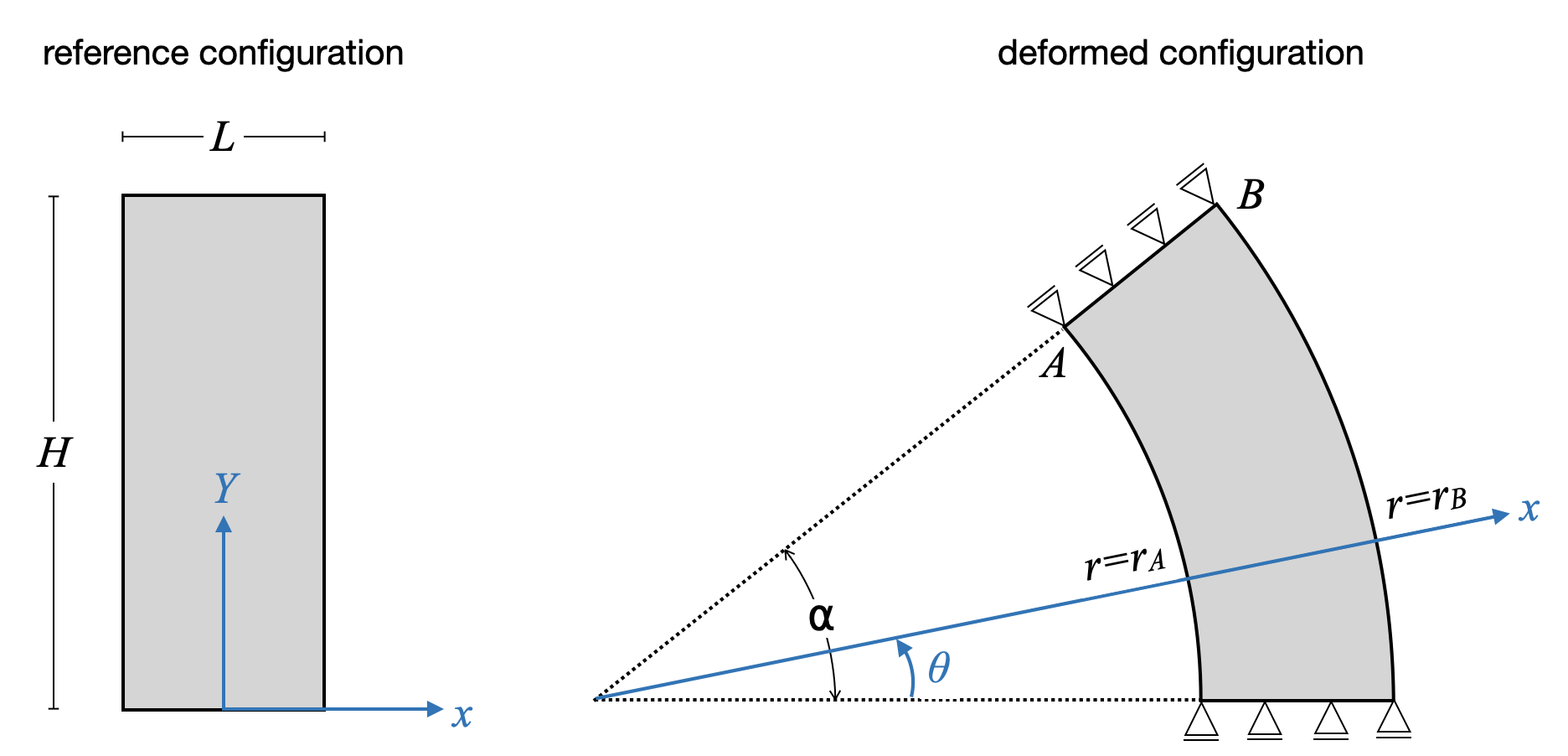
Figure 3: Schematic of the geometry and boundary conditions adopted for the bending of a rectangular block.

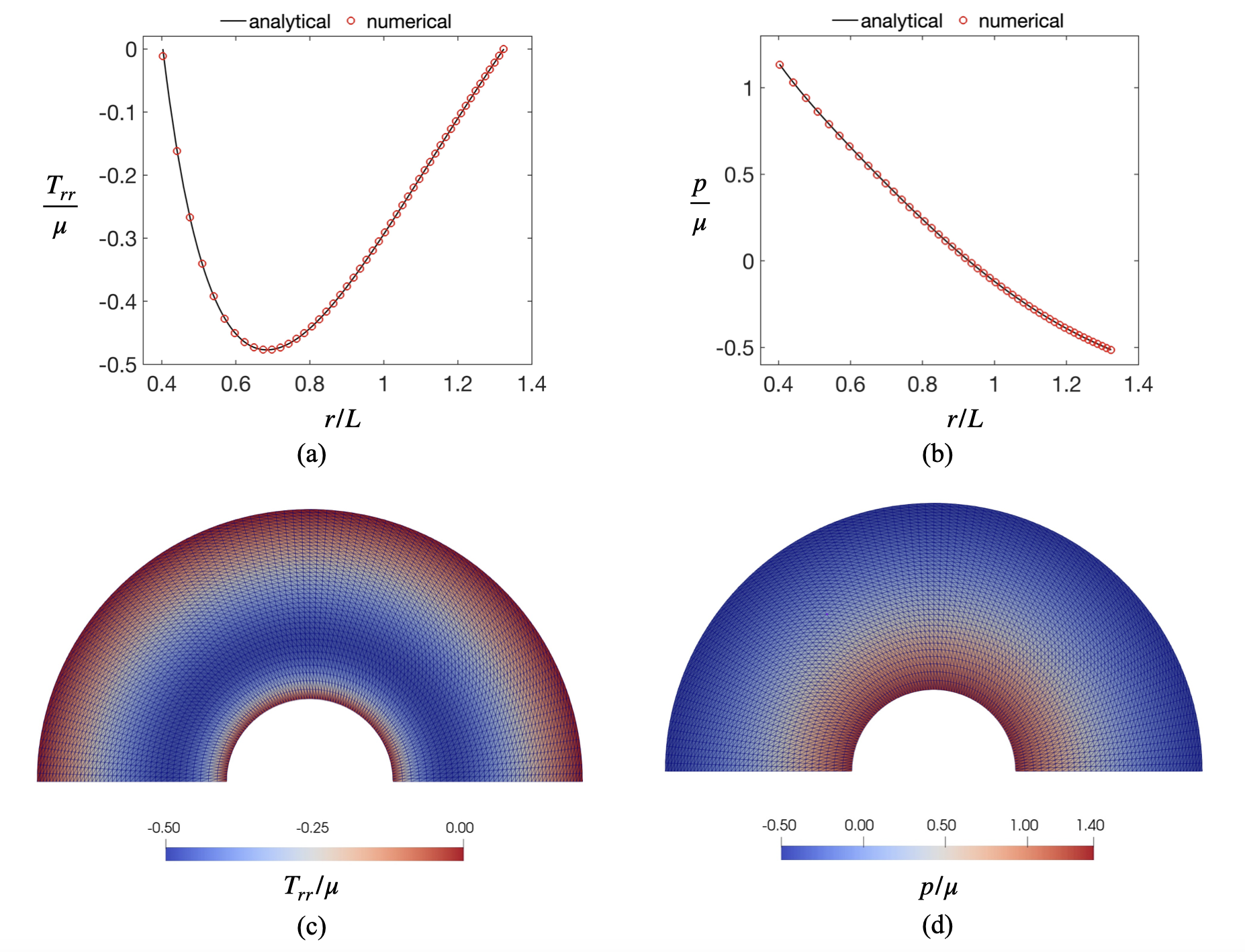
Figure 4: Bending of a rectangular block with initial stress: validation of the proposed numerical implementation using the Finite Element Method. (a-b) Plot of the normalized radial stress $T_{rr}/\mu$ and hydrostatic pressure $p/\mu$ against the radial coordinate $r$ for both the analytical and numerical solutions. (c-d) Spatial distribution of the normalized radial stress and hydrostatic pressure in the deformed configuration for the adopted finite element mesh.

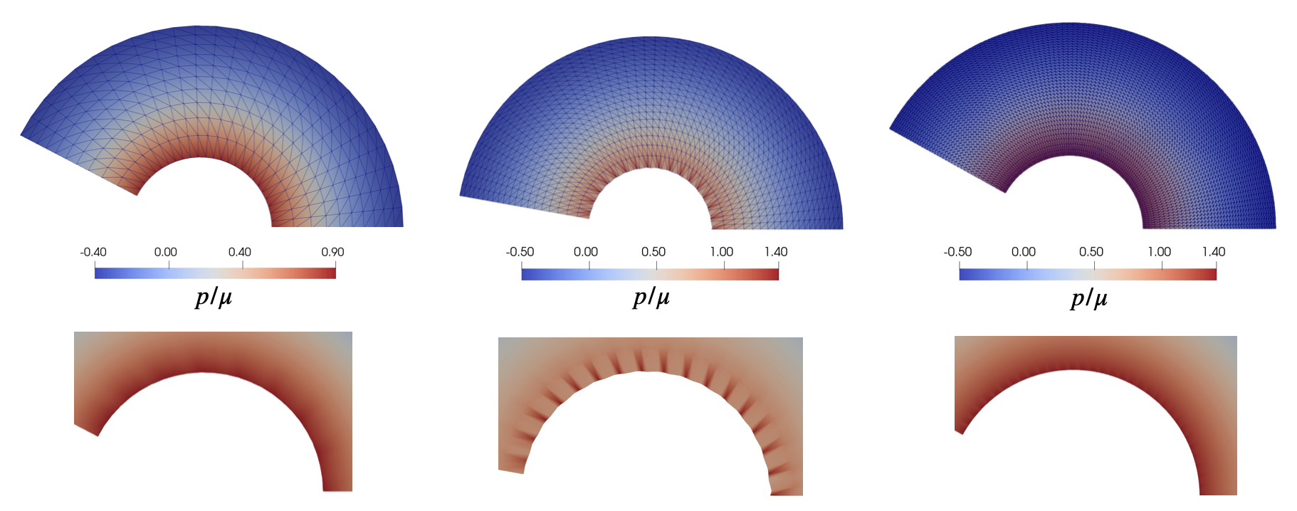
Figure 5: Bending of a rectangular block with initial stress: numerical results obtained using a standard model formulation without volumetric/deviatoric splitting. (Top) Simulated spatial distribution of the normalized hydrostatic pressure for three different finite element meshes. The reported results refer to the last simulated load increment before the algorithm fails to converge. (Bottom) Magnification of the pressure distribution in the inner radius showing the typical mesh dependent fluctuations resulting from volumetric locking.

For the sake of model validation, we compare the analytical solution with the one obtained by numerical approximation of the governing equations. In particular, we implemented the model equations into the open-source computing platform FEniCS [34] for their numerical resolution through the Finite Element Method. The geometry and boundary condition of the problem are depicted in Fig. 3. To handle the prescribed bending deformation, we impose the angle between the x-axis and side AB incrementally till its magnitude equals $\alpha$. Operationally, we impose such a constraint in a variational manner through the introduction of an ad-hoc boundary Lagrange multiplier by using the multiphenics library [2]. Therefore, the overall finite element formulation accounts for three independent variables, i.e. the displacement field $\boldsymbol{u}$, the hydrostatic pressure $p$, and the boundary Lagrange multiplier $\lambda$. We approximate $\boldsymbol{u}$ and $\lambda$ with second order elements and $p$ with first order elements.

Figs. 4a-b plots the resulting radial stress $T_{rr}$ and hydrostatic pressure $p$ against the radial coordinate $r$ for both the numerical and analytical solutions. We observe an excellent agreement between the two solutions, thus demonstrating the correctness of the proposed formulation. We also report the spatial distribution of $T_{rr}$ and $p$ in the deformed configuration in Figs. 4c-d for the adopted finite element mesh. As expected, the considered stress components distributes in space following a cylindrical symmetry.

The proposed formulation actually outperforms the conventional models for initially stressed Neo-Hookean materials as shown in Fig. 5. Here, we gather the numerical outcomes for three different finite element meshes obtained from a standard Neo-Hookean model without resorting to the volumetric/deviatoric splitting proposed in this paper. Such a formulation is unable to capture the imposed bending deformation since the algorithm fails to converge before reaching the final load increment. Lack of numerical convergence follows from spurious volumetric locking as visible in the simulated spatial distribution of the normalized hydrostatic pressure near the inner radius (see bottom of Fig. 5).

6 Concluding Remarks

In this study, we delved into critical aspects associated with the modelling of initially stressed materials, specifically focusing on a class of materials meeting two essential conditions:

1. We required invertibility of the response function $\mathsf{T}_{0}(\mathsf{F}_{\text{e}})$ for the relaxed material, as elucidated in Section 2.2 (see Remark 2.1 for further discussion on this invertibility).

2. We explored materials wherein the initial stress arises from an elastic distortion.

Our investigation highlighted the necessity for the invertibility of $\mathsf{T}_{0}(\mathsf{F}_{\text{e}})$ to properly define $\widehat{\mathsf{T}}(\mathsf{F},\,\mathsf{\Upsigma})$. Moreover, we demonstrated that the commonly imposed initial stress reference independence and initial stress compatibility condition stem naturally from the above two assumptions. While (A1) is a prerequisite for defining $\widehat{\mathsf{T}}(\mathsf{F},\,\mathsf{\Upsigma})$, (A2) may not hold in certain materials where stress formation is accompanied by a change in material properties, as discussed in [42].

Drawing inspiration from Hoger’s work [20], we derived the general expression of the strain energy density $\widehat{\psi}(\mathsf{F},\,\mathsf{\Upsigma})$ for materials satisfying (A1)-(A2). Notably, our analysis revealed that $\widehat{\psi}(\mathsf{F},\,\mathsf{\Upsigma})$ may depend on $I_{5}$ and $I_{7}$ only if $\psi_{0}$ is a function of $II(\mathsf{B}_{\text{e}})$.

We then focused on incompressible media, demonstrating that the strain energy density can be expressed in terms of the deviatoric part of the initial stress tensor $\mathsf{\Upsigma}$ (denoted as $\mathsf{\Upsigma}_{\text{d}}$) and the isochoric part of deformation $\overline{\mathsf{F}}$. This volumetric-deviatoric splitting enabled a reduction of necessary invariants by one compared to existing models.

To illustrate the applicability of our approach, we applied it to an incompressible neo-Hookean material (see (44)). Additionally, we examined the bending of an initially stressed rectangular block, obtaining an analytical solution. The numerical simulations demonstrated that the volumetric-deviatoric splitting of energy exhibited superior performance over the original formulation based on the energy proposed by [14], eliminating locking phenomena and aligning perfectly with the theoretical solution.

The outcomes of this research contribute to the modelling of initially stressed materials, including biological tissues and gels. The proposed volumetric-deviatoric splitting of the energy density holds significant potential in computational mechanics, offering a substantial enhancement to existing methodologies.

Funding

DR gratefully acknowledge the support provided by the European Union – NextGenerationEU under the National Recovery and Resilience Plan (NRRP), Mission 4 Component 2 Investment 1.1 - Call PRIN 2022 No. 104 of February 2, 2022 of Italian Ministry of University and Research; Project 202249PF73 (subject area: PE - Physical Sciences and Engineering) “Mathematical models for viscoelastic biological matter”. MM gratefully acknowledge the support provided by the European Commission through FSE REACT-EU funds, PON Ricerca e Innovazione.

Appendix A Expression of $\det\mathsf{P}\mathsf{P}^{T}$ in terms of $\mathcal{I}_{\mathsf{\Upsigma}}$

To start with, we conveniently indicate with $\mathsf{A}=\mathsf{P}\mathsf{P}^{T}$. By application of the Cayley-Hamilton theorem, we get

$$-\mathsf{A}^{3}+\operatorname{tr}(\mathsf{A})\,\mathsf{A}^{2}-II(\mathsf{A})+\det(\mathsf{A})\mathsf{I}=\mathsf{0}\,,$$

and, by taking the trace at both sides along with exploiting the definition of $II(\mathsf{A})$, it results

$$\det(\mathsf{A})=\frac{1}{3}\left(\operatorname{tr}(\mathsf{A}^{3})-\operatorname{tr}(\mathsf{A})\,\operatorname{tr}(\mathsf{A}^{2})+\operatorname{tr}(\mathsf{A})\frac{\operatorname{tr}(\mathsf{A})^{2}-\operatorname{tr}(\mathsf{A}^{2})}{2}\right)\,.$$ (58)

To express (58) in terms of $\mathcal{I}_{\mathsf{\Upsigma}}$, we exploit (13), from which it results, after some manipulations,

$$\operatorname{tr}(\mathsf{A})=3\beta_{0}+\beta_{1}\operatorname{tr}(\mathsf{\Upsigma})+\beta_{2}(\operatorname{tr}(\mathsf{\Upsigma})^{2}-2II(\mathsf{\Upsigma}))\,,$$

$$\operatorname{tr}(\mathsf{A}^{2})=3\beta_{0}^{2}+(\beta_{1}^{2}+2\beta_{0}\beta_{2})\left(\operatorname{tr}(\mathsf{\Upsigma})^{2}-2II(\mathsf{\Upsigma})\right)+\beta_{2}^{2}\operatorname{tr}(\mathsf{\Upsigma}^{4})+2\beta_{0}\beta_{1}\operatorname{tr}(\mathsf{\Upsigma})+2\beta_{1}\beta_{2}\operatorname{tr}(\mathsf{\Upsigma}^{3})\,,$$

$$\operatorname{tr}(\mathsf{A}^{3})=3\beta_{0}^{3}+3\beta_{0}^{2}\beta_{1}\operatorname{tr}(\mathsf{\Upsigma})+3\beta_{0}(\beta_{1}^{3}+\beta_{2})\left(\operatorname{tr}(\mathsf{\Upsigma})^{2}-2II(\mathsf{\Upsigma})\right)+\beta_{1}^{3}\operatorname{tr}(\mathsf{\Upsigma}^{3})$$

$$+3\beta_{2}(\beta_{0}\beta_{2}+\beta_{1}^{2})\operatorname{tr}(\mathsf{\Upsigma}^{4})+3\beta_{1}\beta_{2}^{2}\operatorname{tr}(\mathsf{\Upsigma}^{5})+\beta_{2}^{3}\operatorname{tr}(\mathsf{\Upsigma}^{6})\,.$$

where $\operatorname{tr}(\mathsf{\Upsigma}^{3})$, $\operatorname{tr}(\mathsf{\Upsigma}^{4})$, $\operatorname{tr}(\mathsf{\Upsigma}^{5})$, and $\operatorname{tr}(\mathsf{\Upsigma}^{6})$ can be recast in therm of $\mathcal{I}_{\mathsf{\Upsigma}}$ by repeatedly using the Cayley-Hamilton theorem for $\mathsf{\Upsigma}$.

References

- [1] E. H. O. Alameen, A. Lucantonio, and A. DeSimone. Mechanics and transient morphing of soft hygroscopic bilayers. Mechanics Research Communications, 131:104131, 2023.
- [2] F. Ballarin. multiphenics website. https://multiphenics.github.io/, 2024. Accessed: February 29, 2024.
- [3] N. Barnafi, F. Regazzoni, and D. Riccobelli. Reconstructing relaxed configurations in elastic bodies: Mathematical formulations and numerical methods for cardiac modeling. Computer Methods in Applied Mechanics and Engineering, 423:116845, 2024.
- [4] J. Bonet and R. D. Wood. Nonlinear continuum mechanics for finite element analysis. Cambridge university press, 1997.
- [5] C.-J. Chuong and Y.-C. Fung. Residual stress in arteries. In Frontiers in biomechanics, pages 117–129. Springer, 1986.
- [6] P. Ciarletta, M. Destrade, and A. Gower. On residual stresses and homeostasis: an elastic theory of functional adaptation in living matter. Scientific Reports, 6:24390, 2016.
- [7] P. Ciarletta, M. Destrade, A. L. Gower, and M. Taffetani. Morphology of residually-stressed tubular tissues: Beyond the elastic multiplicative decomposition. Journal of the Mechanics and Physics of Solids, 90:242–253, 2016.
- [8] V. Damioli, E. Zorzin, A. DeSimone, G. Noselli, and A. Lucantonio. Transient shape morphing of active gel plates: geometry and physics. Soft Matter, 18(31):5867–5876, 2022.
- [9] E. A. de Souza Neto, D. Peric, and D. R. J. Owen. Computational methods for plasticity: theory and applications. John Wiley & Sons, 2011.
- [10] Y. Du, C. Lü, W. Chen, and M. Destrade. Modified multiplicative decomposition model for tissue growth: beyond the initial stress-free state. Journal of the Mechanics and Physics of Solids, 118:133–151, 2018.
- [11] M. Epstein. The Elements of Continuum Biomechanics. Wiley, 2012.
- [12] M. Epstein. Mathematical characterization and identification of remodeling, growth, aging and morphogenesis. Journal of the Mechanics and Physics of Solids, 84:72–84, 2015.
- [13] A. Goriely. The mathematics and mechanics of biological growth, volume 45. Springer, 2017.
- [14] A. L. Gower, P. Ciarletta, and M. Destrade. Initial stress symmetry and its applications in elasticity. Proceedings of the Royal Society A: Mathematical, Physical and Engineering Sciences, 471(2183):20150448, 2015.
- [15] A. L. Gower, T. Shearer, and P. Ciarletta. A new restriction for initially stressed elastic solids. The Quarterly Journal of Mechanics and Applied Mathematics, 70(4):455–478, 2017.
- [16] A. L. Gower, T. Shearer, P. Ciarletta, and M. Destrade. Restriction on stored energy functions that depend on initial stress or strain. in preparation.
- [17] M. E. Gurtin, E. Fried, and L. Anand. The Mechanics and Thermodynamics of Continua. Cambridge University Press, 2010.
- [18] A. Hoger. On the residual stress possible in an elastic body with material symmetry. Archive for Rational Mechanics and Analysis, 88:271–289, 1985.
- [19] A. Hoger. On the determination of residual stress in an elastic body. Journal of Elasticity, 16:303–324, 1986.
- [20] A. Hoger. The constitutive equation for finite deformations of a transversely isotropic hyperelastic material with residual stress. Journal of Elasticity, 33:107–118, 1993.
- [21] A. Hoger. Residual stress in an elastic body: a theory for small strains and arbitrary rotations. Journal of Elasticity, 31:1–24, 1993.
- [22] A. Hoger. The elasticity tensor of a transversely isotropic hyperelastic material with residual stress. Journal of Elasticity, 42:115–132, 1996.
- [23] A. Hoger. On rayleigh-type surface waves in an initially stressed incompressible elastic solid. IMA Journal of Applied Mathematics, 79:360––376, 2012.
- [24] G. A. Holzapfel. Nonlinear Solid Mechanics: a Continuum Approach for Engineering Science. 2000.
- [25] G. A. Holzapfel. Nonlinear solid mechanics: a continuum approach for engineering science, 2002.
- [26] G. A. Holzapfel and R. W. Ogden. Modelling the layer-specific three-dimensional residual stresses in arteries, with an application to the human aorta. Journal of the Royal Society Interface, 7(46):787–799, 2010.
- [27] R. Huang, R. W. Ogden, and R. Penta. Mathematical modelling of residual-stress based volumetric growth in soft matter. Journal of Elasticity, 145(1-2):223–241, 2021.
- [28] B. Johnson and A. Hoger. The dependence of the elasticity tensor on residual stress. Journal of Elasticity, 33:145–165, 1993.
- [29] B. Johnson and A. Hoger. The use of a virtual configuration in formulating constitutive equations for residually stressed elastic materials. Journal of Elasticity, 41:177–215, 1995.
- [30] B. E. Johnson and A. Hoger. The use of strain energy to quantify the effect of residual stress on mechanical behavior. Mathematics and Mechanics of Solids, 3:447–470, 1998.
- [31] D. A. Koss and S. M. Copley. Thermally induced residual stresses in eutectic composites. Metallurgical Transactions, 2:1557–1560, 1971.
- [32] G.-Y. Li, A. L. Gower, and M. Destrade. An ultrasonic method to measure stress without calibration: The angled shear wave method. The Journal of the Acoustical Society of America, 148(6):3963–3970, 2020.
- [33] T. Y. Lin and N. H. Burns. Design of Prestressed Concrete Structures (Third ed.). 1981.
- [34] A. Logg, Mardal, K.A., and G. Wells. Automated Solution of Differential Equations by the Finite Element Method. Springer, 2012.
- [35] J. Merodio, R. Ogden, and J. Rodríguez. The influence of residual stress on finite deformation elastic response. International Journal of Non-Linear Mechanics, 56:43–49, 2013.
- [36] E. Moghimi, A. R. Jacob, and G. Petekidis. Residual stresses in colloidal gels. Soft Matter, 13(43):7824–7833, 2017.
- [37] N. T. Nam, J. Merodio, R. W. Ogden, and P. C. Vinh. The effect of initial stress on the propagation of surface waves in a layered half-space. International Journal of Solids and Structures, 88-89:88–100, 2016.
- [38] W. Noll. Materially uniform simple bodies with inhomogeneities. Archive for Rational Mechanics and Analysis, 27(1):1–32, 1967.
- [39] R. W. Ogden. Non-linear elastic deformations. Courier Corporation, 1997.
- [40] R. W. Ogden. Change of reference configuration in nonlinear elasticity: Perpetuation of a basic error. Mathematics and Mechanics of Solids, 28(9):2132–2138, 2023.
- [41] W. J. Parnell, A. N. Norris, and T. Shearer. Employing pre-stress to generate finite cloaks for antiplane elastic waves. Applied Physics Letters, 100(17):171907, 2012.
- [42] D. Riccobelli, A. Agosti, and P. Ciarletta. On the existence of elastic minimizers for initially stressed materials. Philosophical Transactions of the Royal Society A: Mathematical, Physical and Engineering Sciences, 377(2144):20180074, mar 2019.
- [43] D. Riccobelli and P. Ciarletta. Shape transitions in a soft incompressible sphere with residual stresses. Mathematics and Mechanics of Solids, 23(12):1507–1524, 2018.
- [44] E. K. Rodriguez, A. Hoger, and A. D. McCulloch. Stress-dependent finite growth in soft elastic tissues. Journal of biomechanics, 27(4):455–467, 1994.
- [45] M. Shams, M. Destrade, and R. W. Ogden. Initial stresses in elastic solids: Constitutive laws and acoustoelasticity. Wave Motion, 48(7):552–567, nov 2011.
- [46] T. Stylianopoulos, J. D. Martin, V. P. Chauhan, S. R. Jain, B. Diop-Frimpong, N. Bardeesy, B. L. Smith, C. R. Ferrone, F. J. Hornicek, Y. Boucher, L. L. Munn, and R. K. Jain. Causes, consequences, and remedies for growth-induced solid stress in murine and human tumors. Proceedings of the National Academy of Sciences, 109(38):15101–15108, 2012.
- [47] A. Sydney Gladman, E. A. Matsumoto, R. G. Nuzzo, L. Mahadevan, and J. A. Lewis. Biomimetic 4D printing. Nature Materials, 15(4):413–418, 2016.
- [48] C. Thiel, J. Voss, R. J. Martin, and P. Neff. Do we need truesdell’s empirical inequalities? on the coaxiality of stress and stretch. International Journal of Non-Linear Mechanics, 112:106–116, June 2019.
- [49] S. White and H. Hahn. Cure cycle optimization for the reduction of processing-induced residual stresses in composite materials. Journal of Composite Materials, 27(14):1352–1378, 1993.
- [50] Z. Zhang, G.-Y. Li, Y. Jiang, Y. Zheng, A. L. Gower, M. Destrade, and Y. Cao. Noninvasive measurement of local stress inside soft materials with programmed shear waves. Science Advances, 9(10):eadd4082, 2023.
- [51] N. Zobeiry and A. Poursartip. 3 - the origins of residual stress and its evaluation in composite materials. In P. W. R. Beaumont, C. Soutis, and A. Hodzic, editors, Structural Integrity and Durability of Advanced Composites, Woodhead Publishing Series in Composites Science and Engineering, pages 43–72. Woodhead Publishing, 2015.
- [52] G. Zurlo and L. Truskinovsky. Printing non-euclidean solids. Physical Review Letters, 119(4):048001, 2017.