Boundary and distributed optimal control for a population dynamics PDE model with discontinuous in time Galerkin FEM schemes

Abstract.

We consider fully discrete finite element approximations for a semilinear optimal control system of partial differential equations in two cases: for distributed and Robin boundary control. The ecological predator-prey optimal control model is approximated by conforming finite element methods mimicking the spatial part, while a discontinuous Galerkin method is used for the time discretization. We investigate the sensitivity of the solution distance from the target function, in cases with smooth and rough initial data. We employ low, and higher-order polynomials in time and space whenever proper regularity is present. The approximation schemes considered are with and without control constraints, driving efficiently the system to desired states realized using non-linear gradient methods.

1. Introduction

We examine an optimal control problem arising from chemical kinetics, biology, and ecology in a two-species formulation. Boundary or distributed control function ($g_{i}$) is applied to a system ($y_{i}$) driving it to a desired target (${y_{i,d}}$), $i=1,2$. We assume the control function space $S$ employed in a set $\Omega\subset\mathbb{R}^{2}$ that denotes an open bounded and convex domain with Lipschitz boundary $\Gamma$. $S=\Omega$ refers to distributed and $S=\Gamma$ to boundary control. The scope of this work is to study the distance between the solution and the desired target function and to investigate how the parameters affect the solutions under the minimization of the quadratic functional

(1.1) $${\color[rgb]{0,0,0}J(y_{1},y_{2},g_{1},g_{2}):=}\left\{\frac{1}{2}\int_{0}^{T}{\left\|y_{1}-{y_{1,d}}\right\|_{L^{2}(\Omega)}^{2}dt}+\frac{\gamma_{1}}{2}\int_{0}^{T}{\left\|g_{1}\right\|_{L^{2}({\bf{S}})}^{2}dt}\right.$$

$$+\left.\frac{1}{2}\int_{0}^{T}{\left\|{{y_{2}-{y_{2,d}}}}\right\|_{L^{2}(\Omega)}^{2})dt}+\frac{\gamma_{2}}{2}\int_{0}^{T}{\left\|g_{2}\right\|_{L^{2}({\bf{S}})}^{2}dt}\right\},$$

subject to the Lotka-Volterra system with distributed control

(1.2) $${{\color[rgb]{0,0,0}{{y_{1t}}}}}=\epsilon_{1}\Delta y_{1}+(a-by_{2})y_{1}+g_{1}+f_{1}{\text{ in }}(0,T]\times\Omega,\quad y_{1}=0{\text{ on }}(0,T]\times\Gamma,\quad$$

(1.3) $${{\color[rgb]{0,0,0}{{y_{2t}}}}}=\epsilon_{2}\Delta y_{2}+(cy_{1}-d)y_{2}+g_{2}+f_{2}{\text{ in }}(0,T]\times\Omega,\quad y_{2}=0{\text{ on }}(0,T]\times\Gamma,$$

or the Lotka-Volterra system with Robin boundary control

(1.4) $${{\color[rgb]{0,0,0}{{y_{1t}}}}}=\epsilon_{1}\Delta y_{1}+(a-by_{2})y_{1}+f_{1}{\text{ in }}(0,T]\times\Omega,\quad{{\color[rgb]{0,0,0}y_{1}}}+\frac{\epsilon_{1}}{\lambda_{1}}\frac{\partial y_{1}}{\partial{\mathbf{n}}}=g_{1}{\text{ on }}(0,T]\times\Gamma,\quad$$

(1.5) $${{\color[rgb]{0,0,0}{{y_{2t}}}}}=\epsilon_{2}\Delta y_{2}+(cy_{1}-d)y_{2}+f_{2}{\text{ in }}(0,T]\times\Omega,\quad y_{2}+\frac{\epsilon_{2}}{\lambda_{2}}\frac{\partial y_{2}}{\partial{\mathbf{n}}}=g_{2}{\text{ on }}(0,T]\times\Gamma,$$

enforcing initial data

$$y_{1}(0,x)={y_{1,0}}\quad y_{2}(0,x)={y_{2,0}}{\text{ in }}\Omega.$$

Within the next paragraphs, we introduce literature and important past works as well as details related to the dynamics of the considered system. We also present the involved parameters and their physical meaning explaining how they affect the solution.

1.1. The physical model and related results

There is a wide variety of Lotka-Volterra system versions, the predator-prey/defense, the competitive/colonization and/or the cooperative/resource exchange systems. In general, the Lotka-Volterra predator-prey model mimics bacteria populations, chemical reactions, and other similar models. In this manuscript, we focus on predator-prey/defense systems in two space dimensions $x_{1}$, $x_{2}$ with two species and concentrations $y_{1}$, $y_{2}$, (1.2)-(1.5). The $y_{1}$ variable describes the prey’s concentration, whereas the $y_{2}$ variable represents the predator’s. The parameters i) $a$ represents the growth rate of $y_{1}$, ii) $b$ represents the rate of $y_{2}$ is killing $y_{1}$, iii) $c$ represents the growth rate of $y_{2}$ by chances of killing $y_{1}$, and iv) $d$ represents the death rate of $y_{2}$, [33]. The forcing terms $f_{1}$, $f_{2}$ and the parameters $\lambda_{1}$, $\lambda_{2}$, $\epsilon_{1}$, $\epsilon_{2}$, are given data while $\gamma_{1}$, $\gamma_{2}$ denote penalty parameters that limit the size of the control and will properly be chosen.

Several results regarding the analysis of related systems have been recorded in the literature. We start with the pioneer works of Holling and Volterra for simple types of predation and parasitism and the response of predators to prey density with its role in mimicry and population regulation, [36, 37, 54]. In [30] fully discrete estimates, a fully discrete error bound, and rates of convergence for systems modeling predator–prey interactions, where the local growth of prey is logistic and the predator displays the Holling type II functional response associated with real kinetics is presented. In [16] high-order schemes for a modified predator-prey system proving main stability estimates, under minimal regularity assumptions on the given data, are considered obtaining a-priori error estimate. In [20] predator–prey Holling type dynamics using implicit-symplectic schemes are analyzed proving optimal a priori error estimates. We also report the books [33], [48], and the references therein, presenting ideas starting from the classical work of [54] and thereafter.

Since Lotka-Volterra systems are considered reaction-diffusion systems models, we report related works resembling the predator-prey system. Such is the discontinuous Galerkin (dG) methods for mass transfer through semi-permeable membranes [8], Brusselator systems [15], and predator–prey models with the addition of cross-diffusion blows-up on surfaces employing an implicit-explicit (IMEX) method [25]. For $\lambda$–$\omega$ type reaction-diffusion systems the interested reader could see [28], for the forced Fisher equation that models the dynamics of gene selection/migration for a diploid population with two available alleles in a multidimensional habitat and in the presence of an artificially introduced genotype [32], error estimates for the semidiscrete Galerkin approximations of the FitzHugh-Nagumo equations [40], and epitaxial fourth order growth model with implicit-explicit time discretization is handled in [42, 45]. The performance of several linear multi-step IMEX schemes for reaction-diffusion problems in pattern formation are discussed in [51], and finite volume element approximation of an inhomogeneous Brusselator model with cross-diffusion are analyzed in [47].

For continuous or dG in space and/or dG in time parabolic PDE discretizations we quote the works [3, 4, 19, 24, 23], while nonlinear parabolic, implicit, and implicit-explicit multistep finite element methods can be found in [2, 1].

In [9], a metaheuristic optimization method based on the Lotka-Volterra system equations where the interaction that exists in nature between plants through a network of fungi, and the Lotka-Volterra system of equations model the different types of relationships, is examined. In [39], the Lotka-Volterra model is investigated as two coupled ordinary differential equations representing the interaction of two species, a prey one and a predator one formulating an optimal control problem by adding the effect of hunting both species as the control variable implementing a single shooting method to solve the optimization problem. Moreover, in [26] the uniqueness of the optimal control is obtained by assuming a large crowding effect of the species.

Optimal control, with PDEs as constraints, works also are [29], where results from semigroup theory and a semi-implicit Galerkin finite element method are employed, based on the kinetics satisfying a Lyapunov-type condition of a nonlinear plankton-fish optimal control reaction-diffusion system. In [14] an optimal control problem for a parabolic PDE also with nonsmooth initial data and discontinuous in time discretization for Robin boundary control and [13, 49] for distributed control associated with semilinear parabolic PDEs are presented, see also references therein. We refer to [31], [12] for fluids control, to [38] for nonsmooth optimal control problems governed by coupled semilinear PDE-ODE systems and [27], [17] for optimal control of time-discrete phase flow driven by diffuse models. More optimal control works are [46] considering elliptic PDE optimal control systems with unfitted mesh approaches based on reduced order modeling techniques, and [5] concerning random geometrical morphings on a cutfem dG type optimal control framework.

The scopes of the present manuscript is to investigate continuous and fully discrete finite element formulations for a semilinear optimal control system of a predator-prey Lotka-Volterra type model. A conforming finite element for the spatial part has been adopted, as well as a discontinuous Galerkin approximation for the time part. Cases with and without control constraints have been considered, and for the handling of distributed or Robin boundary optimal controls, non-linear gradient methods have been employed. A study is presented on the sensitivity of the solution distance from the target function in cases with smooth and rough initial data. Numerical tests are conducted to illustrate the effectiveness of the approach and its robustness with respect to the regularity of the initial data, as well as, from the space and/or time higher order polynomial approximation point of view whenever it is applicable. The aforementioned numerical experiments in cases of distributed and boundary controls and implemented with the FreeFem++ software, show also the effect of control constraints. In both distributed and boundary controls several results have been reported with respect to the distance from the targets, with smooth and non smooth initial conditions, and also the effects of controls on the optimal state solutions are presented.

The necessary and sufficient conditions characterized by first and second derivative of the cost functions have been introduced with a proof of the challenging case of constrained in specific intervals optimal control. Furthermore, some extended standard but necessary results have been presented.

The document is organized as follows. In Section 1, the continuous system in a strong formulation is introduced while in Section 2, related results and theoretical tools and preliminaries are presented for the continuous and discretized formulation. In Section 3, the continuous and discretized weak form in the dG in time framework and the optimality system is reported while distributed control is applied with control constraints. Additionally, the first-order optimality conditions are demonstrated and the second-order optimality conditions and sufficient conditions for optimality are proved. In the following, in Section 4 we extend the study to Robin boundary control, we introduce the optimality system and the fully discrete Robin boundary type optimal control problem.

Finally, in Section 5 several numerical experiments expose tables reporting results for the distance norm for the two species and $J$ functional values, for the distributed control case: ($\alpha$) with control constraints and constant polynomials in time and linear in space, ($\beta$) without control constraints and linear in time, quadratic in space, and ($\gamma$) a qualitative study and nullclines are presented. For the boundary Robin control case: low regularity initial data employing constant in time/linear in space polynomials, as well as linear in time/linear in space, linear in time/quadratic in space polynomials and the heuristic control algorithm used are demonstrated.

To our best knowledge, there are no predator-prey related investigations considering discontinuous Galerkin in time in which optimal control techniques are applied with low and higher order dG in time discretization, as well as with non-smooth data, and the manuscript provides a contribution in the field indicating a strategy that can be extended to more complicated situations.

2. Background

2.1. Notation

Following the literature, see e.g. [22, Chapter 5], we use the Hilbert spaces standard notation $L^{2}(\Omega)$, $H^{s}(\Omega)$, $0<s\in\mathbb{R}$, $H^{1}_{0}(\Omega)\equiv\{v\in H^{1}(\Omega):v|_{\Gamma}=0\}$. We denote by $H^{-1}(\Omega)$ the dual of $H^{1}_{0}(\Omega)$, $H^{*}(\Omega)$ the dual of $H^{1}(\Omega)$ and the corresponding duality pairing by $\langle\cdot,\cdot\rangle_{H^{1}(\Omega)^{*},H^{1}(\Omega)}\equiv\langle\cdot,\cdot\rangle$. We will frequently use the space $H^{1/2}(\Gamma)$, its dual denoted by $H^{-1/2}(\Gamma)$, and their duality pairing denoted by $\langle.,.\rangle_{H^{-1/2}(\Gamma),H^{1/2}(\Gamma)}\equiv\langle\cdot,\cdot\rangle_{\Gamma}$. Finally, the standard notation $(\cdot,\cdot)$, $(\cdot,\cdot)_{\Gamma}$ will be used for the $L^{2}(\Omega)\equiv H^{0}(\Omega)$ and $L^{2}(\Gamma)$ inner products respectively. For any of the above Sobolev spaces, we define the space-time spaces in a standard way.

For any Banach space $X$, we denote by $L^{p}[0,T;X],L^{\infty}[0,T;X]$ the standard time-space spaces, endowed with norms:

$$\|v\|_{L^{p}[0,T;X]}=\left(\int_{0}^{T}\|v\|^{p}_{X}dt\right)^{\frac{1}{p}},\quad\|v\|_{L^{\infty}[0,T;X]}=\mbox{ ess$\sup_{t\in[0,T]}\|v\|_{X}$}.$$

The set of all continuous functions $v:[0,T]\rightarrow X$, is denoted by $C[0,T;X]$, with norm defined by $\|v\|_{C[0,T;X]}=\max_{t\in[0,T]}\|v(t)\|_{X}.$ Finally, we denote in a classic way $H^{1}[0,T;X]$ and the norm,

$$\|v\|_{H^{1}[0,T;X]} = \left(\int_{0}^{T}\|v\|^{2}_{X}dt\right)^{\frac{1}{2}}+\left(\int_{0}^{T}\|v_{t}\|^{2}_{X}dt\right)^{\frac{1}{2}}\leq C<\infty.$$

We will frequently use the spaces for the aforementioned system applying distributed control and zero Dirichlet conditions $W_{D}(0,T):=L^{2}[0,T;H^{1}(\Omega)]\cap L^{\infty}[0,T;L^{2}(\Omega)]$ with norm defined as $\|u\|_{W_{D}(0,T)}^{2}\equiv\|u\|_{L^{2}[0,T;H^{1}(\Omega)]}^{2}+\|u\|_{L^{\infty}[0,T;L^{2}(\Omega)]}^{2}$ while for problems employing Robin boundary control $W_{R}(0,T):=L^{2}[0,T;H^{1}(\Omega)]\cap L^{\infty}[0,T;L^{2}(\Omega)]\times L^{2}[0,T;L^{2}(\Gamma)]$ with norm defined as $\|u\|_{W_{R}(0,T)}^{2}\equiv\|u\|_{L^{2}[0,T;H^{1}(\Omega)]}^{2}+\|u\|_{L^{\infty}[0,T;L^{2}(\Omega)]}^{2}+\|u\|_{L^{2}[0,T;L^{2}(\Gamma)]}^{2}$, see e.g. [14], [13].

2.2. Preliminaries and discretization tools

We consider a family of triangulations, $\{\mathcal{T}_{h}\}_{h>0}$ of $\Omega$, defined in the standard way, [11]. We associate two parameters $h_{T}$ and $\rho_{T}$ for each element $T\in\mathcal{T}_{h}$, denoting the diameter of the set $T$, and the diameter of the largest ball contained in $T$ respectively. The size of the mesh is denoted by $h=\max_{T\in\mathcal{T}_{h}}h_{T}$. The following standard properties of the mesh will be assumed: $\alpha)$ There exist two positive constants $\rho_{\mathcal{T}}$ and $\delta_{\mathcal{T}}$ such that $\frac{h_{T}}{\rho_{T}}\leq\rho_{\mathcal{T}}\ \mbox{ and }\ \frac{h}{h_{T}}\leq\delta_{\mathcal{T}}\ \ \forall T\in\mathcal{T}_{h}\mbox{ and }\forall h>0,$ $\beta)$ Given $h$, let $\{T_{j}\}_{j=1}^{N_{h}}$ denote the family of triangles belonging to $\mathcal{T}_{h}$ and having one side included on the boundary $\Gamma$. Thus, if the vertices of $T_{j}\cap\Gamma$ are denoted by $x_{j,\Gamma}$, $x_{j+1,\Gamma}$ then the straight line $[x_{j,\Gamma},x_{j+1,\Gamma}]\equiv T_{j}\cap\Gamma$. Here, we also assume that $x_{1,\Gamma}=x_{N_{h}+1,\Gamma}$.

Considering the mesh $\mathcal{T}_{h}$ we construct the finite dimensional spaces $U_{h,{{D}}}\subset H^{1}_{0}(\Omega)$, $U_{h,{{R}}}\subset H^{1}(\Omega)$ employing piecewise polynomials in $\Omega$. Standard approximation theory assumptions are assumed on these spaces. In particular, for any $v\in H^{l+1}(\Omega)$, there exists an integer $\ell\geq 1$, and a constant $C>0$ independent of $h$ such that: $\inf_{v_{h}\in U_{h}}\|v-v_{h}\|_{H^{s}(\Omega)}\leq Ch^{l+1-s}\|v\|_{H^{l+1}(\Omega)},\ \mbox{ for }0\leq l\leq\ell\mbox{ and }s=-1,0,1,$ and inverse inequalities on quasi-uniform triangulations, i.e., there exist constants $C\geq 0$, such that $\|v_{h}\|_{H^{1}(\Omega)}\leq C/h\|v_{h}\|_{L^{2}(\Omega)}$, and $\|v_{h}\|_{L^{2}(\Omega)}\leq C/h\|v_{h}\|_{H^{1}(\Omega)^{*}}$. Fully discrete approximations will be constructed on a quasi-uniform partition $0=t^{0}<t^{1}<\ldots<t^{N}=T$ of $[0,T]$, i.e., there exists a constant $0<\theta<1$ such that $\min_{n=1,..,N}(t^{n}-t^{n-1})\geq\theta\max_{n=1,...,N}(t^{n}-t^{n-1})$. We also use the notation $\tau^{n}=t^{n}-t^{n-1},\tau=\max_{n=1,...,N}\tau^{n}$ and we denote by ${\mathcal{P}}_{k}[t^{n-1},t^{n};U_{{h{{,D}}}}\text{ or }U_{{h{{,R}}}}]$ the space of polynomials of degree $k$ or less, having values in $U_{{h{{\color[rgb]{0,0,0},D}}}}$ or $U_{{h{{\color[rgb]{0,0,0},R}}}}$. We seek approximate solutions belonging to the spaces

$${\mathcal{U}}_{h,{{\color[rgb]{0,0,0}D}}}=\{y_{ih}\in L^{2}[0,T;H^{1}_{0}(\Omega)]:y_{ih}|_{(t^{n-1},t^{n}]}\in{\mathcal{P}}_{k}[t^{n-1},t^{n};U_{h,{{D}}}]\},$$

$${\mathcal{U}}_{h,{{\color[rgb]{0,0,0}R}}}=\{y_{ih}\in L^{2}[0,T;H^{1}(\Omega)]:y_{ih}|_{(t^{n-1},t^{n}]}\in{\mathcal{P}}_{k}[t^{n-1},t^{n};U_{h,{{\color[rgb]{0,0,0}R}}}]\}.$$

By convention, the functions of ${{\mathcal{U}}_{h,{{\color[rgb]{0,0,0}D}}}}$, ${{\mathcal{U}}_{h,{{\color[rgb]{0,0,0}R}}}}$ are left continuous with right limits and hence will write $y^{n}_{ih}\equiv y^{n}_{{ih}-}$ for $y_{ih}(t^{n})=y_{ih}(t^{n}_{-})$, and $y^{n}_{{ih}+}$ for $y_{ih}(t^{n}_{+})$, while the jump at $t^{n}$, is denoted by $[y^{n}_{ih}]=y^{n}_{{ih}+}-y^{n}_{{ih}}$. In the above definitions, we have used the following notational abbreviation, $y_{{ih},\tau}\equiv y_{ih}$, ${\mathcal{U}}_{h,\tau,{{\color[rgb]{0,0,0}D}}}\equiv{\mathcal{U}}_{h,{{\color[rgb]{0,0,0}D}}}$, ${\mathcal{U}}_{h,\tau,{{\color[rgb]{0,0,0}R}}}\equiv{\mathcal{U}}_{h,{{\color[rgb]{0,0,0}R}}}$. For the time discretization, we will use the lowest order scheme ($k=0$) which corresponds to the discontinuous Galerkin variant of the implicit Euler. This approach gives good results also in cases with limited regularity which is acting as a barrier in terms of developing estimates of higher order. Although, we will illustrate some cases related to higher-order schemes. The discretization of the control can be effectively achieved through the discretization of the adjoint variable $\mu$. However, we point out that the only regularity assumption on the discrete control is $g_{1h},g_{2h}\in L^{2}[0,T;L^{2}(\Omega)]$ or $g_{1h},g_{2h}\in L^{2}[0,T;L^{2}(\Gamma)]$ for the distributed and boundary control respectively.

3. Distributed control, Dirichlet zero boundary and control constraints.

This section is devoted to distributed control with Dirichlet zero boundary, the enriched problem actually involves the functional $J(y_{1},y_{2},g_{1},g_{2})$ as it is described in (1.1) for $S=\Omega$, subject to the control constraints

$$g_{ia}\leq g_{i}(t,x)\leq g_{ib}\text{ for a.e.}(t,x)\in(0,T)\times\Omega\text{, where}\,\,{g_{ia}},{g_{ib}}\in{\mathbb{R}},\,\,i=1,2.$$

3.1. The continuous and discrete control problem/optimality system

Below, we state the optimality system which consists of the state equation given in the weak form, the adjoint, and the optimality condition applying distributed control. Particularly, first-order necessary conditions (optimality system) of the above optimal control problems are demonstrated. The aforementioned systems are introduced by employing a discontinuous in time Galerkin (dG) scheme and a conforming Galerkin method in space. The corresponding optimality system (first-order necessary conditions) consists of a primal (forward in time) equation system and an adjoint (backward in time) equation system which are coupled through an optimality condition, and non-linear terms as it is described in Lemma 3.3. The main aim is to show that the dG approximations of the optimality system exhibit good behavior and to examine the crucial matter of the distance of the solution from the desired target.

We begin by stating the weak formulation of the state equation. Given $f_{1}$, $f_{2}\in L^{2}\left[0,T;H^{-1}(\Omega)\right]$, controls $g_{1},g_{2}\in L^{2}\left[0,T;L^{2}(\Omega)\right]$, and initial states ${y_{1,0}}$, ${y_{2,0}}\in L^{2}(\Omega)$ we seek $y_{1},y_{2}\in L^{\infty}[0,T;L^{2}(\Omega)]\cap L^{2}[0,T;H_{0}^{1}(\Omega)]$ such that for a.e. $t\in(0,T]$, and for all $v\in H^{1}(\Omega)$

$$\left\langle{{{\color[rgb]{0,0,0}y_{1t}}},v}\right\rangle+\epsilon_{1}(\nabla y_{1},\nabla v)-((a-by_{2})y_{1},v)=\left\langle{f_{1},v}\right\rangle+\left<{g_{1},v}\right>\quad\mbox{ and}\quad\left({y_{1}(0),v}\right) = \left({{y_{1,0}},v}\right),$$

$$\left\langle{{\color[rgb]{0,0,0}{y_{2t}}},v}\right\rangle+\epsilon_{2}(\nabla y_{2},\nabla v)-((cy_{1}-d)y_{2},v)=\left\langle{f_{2},v}\right\rangle+\left<g_{2},v\right>\quad\mbox{ and}\quad\left({y_{2}(0),v}\right) = \left({{y_{2,0}},v}\right).$$

An equivalent well-posed weak formulation which is more suitable for the analysis of dG schemes is to seek $y_{1},y_{2}\in{\color[rgb]{0,0,0}W_{D}(0,T)=L^{2}[0,T;H^{1}(\Omega)]\cap L^{\infty}[0,T;L^{2}(\Omega)]}$ such that for all $v\in L^{2}[0,T;H^{1}(\Omega)]\cap H^{1}[0,T;H^{-1}(\Omega)]$,

$$(y_{1}(T),v(T))+\int_{0}^{T}{\left({-\left\langle{y_{1},v_{t}}\right\rangle+\epsilon_{1}\left({\nabla y_{1},\nabla v}\right)-\left({(a-by_{2})y_{1},v}\right)}\right)}dt$$

(3.1) $$\qquad=({y_{1,0}},v(0))+\int_{0}^{T}{{\left\langle{f_{1},v}\right\rangle}}dt+\int_{0}^{T}{\left({g_{1},v}\right)}dt,$$

$$(y_{2}(T),v(T))+\int_{0}^{T}{\left({-\left\langle{y_{2},v_{t}}\right\rangle+\epsilon_{2}\left({\nabla y_{2},\nabla v}\right)-({(cy_{1}-d)y_{2},v})}\right)}dt$$

(3.2) $$\qquad=({y_{2,0}},v(0))+\int_{0}^{T}{{\left<f_{2},v\right>}}dt+\int_{0}^{T}{\left({g_{2},v}\right)}dt.$$

The control to state mapping $G:L^{2}[0,T;{L^{2}(\Omega)\times L^{2}(\Omega)]}\to W_{D}(0,T)\times W_{D}(0,T)$, which associates to each control $g_{1},g_{2}$ the corresponding state $G(g_{1},g_{2})$ $=({y}_{g_{1}},{y}_{g_{2}})$ $\equiv$ $({\color[rgb]{0,0,0}y_{1}(g_{1},g_{2})},{\color[rgb]{0,0,0}y_{2}(g_{1},g_{2})})$ via (3.1)–(3.2) is well defined, and continuous, so does the cost functional, frequently denoted to by its reduced form, $J(y_{1},y_{2},g_{1},g_{2})\equiv J({\color[rgb]{0,0,0}y_{1}(g_{1},g_{2})},{\color[rgb]{0,0,0}y_{2}(g_{1},g_{2})}):L^{2}[0,T;{L^{2}(\Omega)}]\to\mathbb{R}$.

Definition 3.1.

Let ${f_{1},f_{2}}\in L^{2}[0,T;H^{-1}(\Omega)]$, ${y_{1,0},y_{2,0}}\in L^{2}(\Omega)$, and ${y_{1,d},y_{2,d}}\in L^{2}[0,T;L^{2}(\Omega)]$, $g_{ia}$, $g_{ib}\in\mathbb{R}$ be given data. Then, the set of admissible controls denoted by ${\mathcal{A}}_{ad}$ for the corresponding distributed control problem with constrained controls takes the form: ${\mathcal{A}}_{ad}=\{{g_{i}}\in L^{2}[0,T;L^{2}(\Omega)]:{{g_{ia}}}\leq{g_{i}}(t,x)\leq{{g_{ib}}},i=1,2\text{ for a.e. }(t,x)\in(0,T)\times\Omega\}.$ The pairs $({\color[rgb]{0,0,0}y_{i}(g_{1},g_{2})},g_{i})\in W_{D}(0,T)\times{\mathcal{A}}_{ad},i=1,2$, is said to be an optimal solution if $J({\color[rgb]{0,0,0}y_{1}(g_{1},g_{2})},{\color[rgb]{0,0,0}y_{2}(g_{1},g_{2})},g_{1},g_{2})\leq J({\color[rgb]{0,0,0}w_{1}(h_{1},h_{2}),w_{2}(h_{1},h_{2}),}h_{1},h_{2})$, for all $(h_{1},h_{2})\in\mathcal{A}_{ad}\times\mathcal{A}_{ad}$, $(w_{1}(h_{1}{\color[rgb]{0,0,0},h_{2}}),w_{2}({\color[rgb]{0,0,0}h_{1},}h_{2}))\in W_{D}(0,T)\times W_{D}(0,T)$ being the solution of problem (3.1)–(3.2) with control functions $(h_{1},h_{2})$.

We will occasionally abbreviate the notation $y_{i}\equiv{y}_{g_{i}}\equiv{y_{i}}({\color[rgb]{0,0,0}g_{1},g_{2}}),i=1,2$. An optimality system of equations can be derived by using standard techniques under minimal regularity assumptions on the given initial data and forcing term; see for instance [13]. Here, we adopt the notation and framework of [10, Section 2]. We first state the basic differentiability property of the cost functional.

Lemma 3.2.

The cost functional $J:L^{2}[0,T;{L^{2}(\Omega)}]\to\mathbb{R}$ is of class $C^{\infty}$ and for every $g_{1},g_{2},y_{1},y_{2}\in L^{2}[0,T;{L^{2}(\Omega)}]$,

$$J^{{}^{\prime}}(g_{1},g_{2})(u_{1},u_{2})=\int_{0}^{T}\int_{\Omega}\Big{(}({\mu_{1}}({\color[rgb]{0,0,0}g_{1},g_{2}})+\gamma_{1}g_{1})u_{1},({\mu_{2}}({\color[rgb]{0,0,0}g_{1},g_{2}})+\gamma_{2}g_{2})u_{2}\Big{)}dxdt,$$

where $\mu_{i}({\color[rgb]{0,0,0}g_{1},g_{2}})\equiv{\mu}_{g_{i}}\in W_{D}(0,T),i=1,2,$ is the unique solution of following problem: For all $v\in L^{2}[0,T;H^{1}(\Omega)]\cap H^{1}[0,T;H^{-1}(\Omega)]$,

$$\int_{0}^{T}{\left({\left\langle{{\mu}_{g_{1}},v_{t}}\right\rangle+\epsilon_{1}\left({\nabla{\mu}_{g_{1}},\nabla v}\right)-((a-by_{g_{2}}){\mu}_{g_{1}},v)}\right)dt}$$

(3.3) $$\qquad\qquad\qquad\qquad\qquad\qquad\qquad\qquad=-({\mu}_{g_{1}}(0),v(0))+\int_{0}^{T}\left({y}_{g_{1}}-y_{1,d},v\right)dt,$$

$$\int_{0}^{T}{\left({\left\langle{{\mu}_{g_{2}},v_{t}}\right\rangle+\epsilon_{2}\left({\nabla{\mu}_{g_{2}},\nabla v}\right)-((c{y}_{g_{1}}-d){\mu}_{g_{2}},v)}\right)dt}$$

(3.4) $$\qquad\qquad\qquad\qquad\qquad\qquad\qquad\qquad=-({\mu}_{g_{2}}(0),v(0))+\int_{0}^{T}\left({y}_{g_{2}}-{y_{2,d}},v\right)dt.$$

where $\mu_{g_{i}}(T)=0$ and $(\mu_{g_{i}})_{t}\in L^{2}[0,T;H^{-1}(\Omega)],i=1,2$.

In the following Lemma, we state the optimality system which consists of the state equation, the adjoint, and the optimality condition.

Lemma 3.3.

Let $(y_{g_{i}},g_{i})\equiv(y_{i},g_{i})\in W_{D}(0,T)\times{\mathcal{A}}_{ad},i=1,2,$ denote the unique optimal pairs of Definition 3.1. Then, there exists an adjoint $\mu_{1},\mu_{2}\in W_{D}(0,T)$ satisfying, $\mu_{1}(T)=\mu_{2}(T)=0$ such that for all $v\in L^{2}[0,T;H^{1}(\Omega)]\cap H^{1}[0,T;H^{-1}(\Omega)]$,

$$(y_{1}(T),v(T))+\int_{0}^{T}{\left({-\left\langle{y_{1},v_{t}}\right\rangle+\epsilon_{1}\left({\nabla y_{1},\nabla v}\right)-\left({(a-by_{2})y_{1},v}\right)}\right)}dt$$

(3.5) $$\qquad\qquad\qquad\qquad\qquad=({y_{1,0}},v(0))+\int_{0}^{T}{{\left\langle{f_{1},v}\right\rangle}}dt+\int_{0}^{T}{\left({g_{1},v}\right)}dt,$$

$$(y_{2}(T),v(T))+\int_{0}^{T}{\left({-\left\langle{y_{2},v_{t}}\right\rangle+\epsilon_{2}\left({\nabla y_{2},\nabla v}\right)}\right)}dt-\int_{0}^{T}{\left((cy_{1}-d)y_{2},v\right)}dt$$

(3.6) $$\qquad\qquad\qquad\qquad\qquad=({y_{2,0}},v(0))+\int_{0}^{T}{{\left<f_{2},v\right>}}dt+\int_{0}^{T}{\left({g_{2},v}\right)}dt,$$

$$\int_{0}^{T}{\left({\left\langle{{\mu}_{1},v_{t}}\right\rangle+\epsilon_{1}\left({\nabla{\mu}_{1},\nabla v}\right)-((a-by_{2}){\mu}_{1},v)}\right)dt}$$

(3.7) $$\qquad\qquad\qquad\qquad\qquad=-({\mu}_{1}(0),v(0))+\int_{0}^{T}\left({y}_{1}-{y_{1,d}},v\right)dt,$$

$$\int_{0}^{T}{\left({\left\langle{{\mu}_{2},v_{t}}\right\rangle+\epsilon_{2}\left({\nabla{\mu}_{2},\nabla v}\right)-((cy_{1}-d){\mu}_{2},v)}\right)dt}$$

(3.8) $$\qquad\qquad\qquad\qquad\qquad=-({\mu}_{2}(0),v(0))+\int_{0}^{T}\left({y}_{2}-{y_{2,d}},v\right)dt,$$

with control constraints:

(3.9) $$\int_{0}^{T}\int_{\Omega}\left(\gamma_{1}g_{1}+\mu_{1}\right)\left(u_{1}-g_{1}\right)dxdt\geq 0,\,\int_{0}^{T}\int_{\Omega}\left(\gamma_{2}g_{2}+\mu_{2}\right)\left(u_{2}-g_{2}\right)dxdt\geq 0,$$

$$\forall u_{1},u_{2}\in{\mathcal{A}}_{ad}.$$

In addition, ${y_{i,t}},{\mu_{i,t}}\in L^{2}[0,T;H^{-1}(\Omega)]$, and note that (3.9), is equivalent to

$$g_{1}(t,x)=Proj_{[{g_{1a}},{g_{1b}}]}\left(-\frac{1}{\gamma_{1}}\mu_{1}(t,x)\right),\,g_{2}(t,x)=Proj_{[{g_{2a}},{g_{2b}}]}\left(-\frac{1}{\gamma_{2}}\mu_{2}(t,x)\right),$$

for a.e. $(t,x)\in(0,T]\times\Omega$, with ${\mu_{i,t}}\in L^{2}[0,T;H^{2}(\Omega)]\cap L^{2}[0,T;L^{2}(\Omega)],i=1,2$.

Proof.

The derivation of the optimality system is standard, see e.g. [52].∎

3.1.1. The fully-discrete distributed optimal control problem

The discontinuous time-stepping fully-discrete scheme for the control to state mapping $G_{{\color[rgb]{0,0,0}h,D}}:L^{2}[0,T;{L}^{2}(\Omega)\times{L}^{2}(\Omega)]\to{\mathcal{U}}_{{\color[rgb]{0,0,0}h,D}}\times{\mathcal{U}}_{{\color[rgb]{0,0,0}h,D}}$, which associates to each control $(g_{1},g_{2})$ the corresponding state $G_{{\color[rgb]{0,0,0}h,D}}(g_{1},g_{2})=({y_{1}}_{g_{1},h},{y_{2}}_{g_{2},h})\equiv(y_{1h}({g_{1}}),y_{2h}({g_{2}}))$ is defined as follows: For any control data $g_{1},g_{2}\in L^{2}[0,T;L^{2}(\Omega)]$, for given initial data ${y_{1,0}},{y_{2,0}}\in L^{2}(\Omega)$, forces $f_{1},f_{2}\in L^{2}[0,T;H^{-1}(\Omega)]$, and targets $y_{1,d}$, $y_{2,d}\in L^{2}[0,T;L^{2}(\Omega)]$ we seek $y_{1h}$, $y_{2h}\in\mathcal{U}_{h}$ such that for $n=1,...,N$, and for all $v_{h}\in{\mathcal{P}}_{k}[t^{n-1},t^{n};U_{{\color[rgb]{0,0,0}h,D}}]$,

$$(y_{1}^{n},v^{n})+\int_{t^{n-1}}^{t^{n}}{\left({-({y_{1h},v_{ht}})+\epsilon_{1}\left({\nabla y_{1h},\nabla v_{h}}\right)-\left((a-by_{2h})y_{1h},v_{h}\right)}\right)}dt$$

(3.10) $$\qquad=({y_{1}}^{n-1},v_{+}^{n-1})+\int_{t^{n-1}}^{t^{n}}{{\left\langle{f_{1},v_{h}}\right\rangle}}dt+\int_{t^{n-1}}^{t^{n}}{\left({g_{1},v_{h}}\right)}dt,$$

$$(y_{2}^{n},v^{n})+\int_{t^{n-1}}^{t^{n}}{\left({-({y_{2h},v_{ht}})+\epsilon_{2}\left({\nabla y_{2h},\nabla v_{h}}\right)}\right)}dt-\int_{t^{n-1}}^{t^{n}}{\left({{(cy_{1h}-d)y_{2h},v_{h}}}\right)}dt$$

(3.11) $$\qquad=({y_{2}}^{n-1},v_{+}^{n-1})+\int_{t^{n-1}}^{t^{n}}{{\left<f_{2},v_{h}\right>}}dt+\int_{t^{n-1}}^{t^{n}}{\left({g_{2},v_{h}}\right)}dt.$$

Remark 3.4.

We note that in the above definition only $g_{1},g_{2}\in L^{2}[0,T;L^{2}(\Omega)]$ regularity is needed to validate the weak fully-discrete formulation. As a matter of fact, the stability estimate at arbitrary time-points as well as in $L^{2}[0,T;H_{0}^{1}(\Omega)]$ norm easily follows by setting $v_{h}=y_{1h}$, $v_{h}=y_{2h}$ into (3.1.1)–(3.11) while for the arbitrary time-points stability estimate, we may apply the techniques as in [14, 13].

Analogously to the continuous case, we will occasionally abbreviate the notation $y_{ih}=y_{ih}(g_{ih})$ and we note that the control to fully-discrete state mapping $G_{{h,D}}:L^{2}[0,T;{{L}}^{2}(\Omega)\times{{L}}^{2}(\Omega)]\to{\mathcal{U}}_{{h,D}}\times{\mathcal{U}}_{{h,D}}$, is well defined, and continuous and let $J_{h}(y_{1h},y_{2h},g_{1h},g_{2h})=\frac{1}{2}\int_{0}^{T}\int_{\Omega}(|y_{1h}-{y_{1,d}}|^{2}+|y_{2h}-{y_{2,d}}|^{2})dxdt+\frac{\gamma_{1}}{2}\int_{0}^{T}\int_{\Omega}(|g_{1h}|^{2})dxdt+\frac{\gamma_{2}}{2}\int_{0}^{T}\int_{\Omega}(|g_{2h}|^{2})dxdt$.

The control problem definition now takes the form:

Definition 3.5.

Let ${\color[rgb]{0,0,0}f_{1},f_{2}}\in L^{2}[0,T;H^{-1}(\Omega)]$, ${\color[rgb]{0,0,0}y_{1,0},y_{2,0}}\in L^{2}(\Omega)$, ${\color[rgb]{0,0,0}y_{1,d},y_{2,d}}\in L^{2}[0,T;L^{2}(\Omega)]$, be given data. Suppose that the set of discrete admissible controls is denoted by ${\mathcal{A}}^{d}_{ad}\equiv{\mathcal{U}}_{{h,D}}\cap{\mathcal{A}}_{ad}$. The pairs $(y_{ih},g_{ih})\in{\mathcal{U}}_{{h,D}}\times L^{2}[0,T;U_{{h,D}}],i=1,2,$ satisfy (3.1.1)–(3.11) and the definition of the corresponding control problem takes the form: The pairs $(y_{ih},g_{ih})\in A^{d}_{ad},i=1,2$, are said to be optimal solutions if $J_{h}(y_{1h},y_{2h},g_{1h},g_{2h})\leq J_{h}(w_{1h},w_{2h},u_{1h},u_{2h})$ for all $(u_{1h},u_{2h})\in\mathcal{A}^{d}_{ad}\times\mathcal{A}^{d}_{ad},(w_{1h},w_{2h})\in\mathcal{U}_{h,D}\times\mathcal{U}_{h,D}$ being the solution of problem (3.1.1)-(3.11) with control functions $(u_{h1},u_{h2})$.

The discrete optimal control problem solution existence can be proved by standard techniques while uniqueness follows from the structure of the functional, and the linearity of the equation. The basic stability estimates in terms of the optimal pair $(y_{ih},g_{ih})\in L^{2}[0,T;H_{0}^{1}(\Omega)]\times L^{2}[0,T;L^{2}(\Omega)],i=1,2,$ can be easily obtained, see e.g. [13].

We note that the key difficulty of the discontinuous time-stepping formulation is the lack of any meaningful regularity for the time-derivative of $y_{ih}$ due to the presence of discontinuities. However, it is also worth noting that dG in time is applicable even for higher order schemes, [13].

3.1.2. The discrete distributed optimality system

In the following Lemmas 3.6 and 3.7 we state the discrete optimality systems in two appropriate forms.

Lemma 3.6.

The cost functional $J_{h}:L^{2}[0,T;{L^{2}(\Omega)}]\to\mathbb{R}$ is well defined differentiable and for every $g_{1},g_{2},u_{1},u_{2}\in L^{2}[0,T;L^{2}(\Omega)]$,

$$J_{h}^{{}^{\prime}}(g_{1},g_{2})(u_{1},u_{2})=\int_{0}^{T}\int_{\Omega}\Big{(}({\mu_{1h}}({g_{1}})+\alpha g_{1})u_{1},({\mu_{2h}}({g_{2}})+\alpha g_{2})u_{2}\Big{)}dxdt,$$

where $\mu_{ih}({g_{i}})\equiv{\mu}_{{g_{i}},h}\in W_{D}(0,T),i=1,2,$ is the unique solution of following problem: For all $\upsilon_{h}\in P_{k}[t^{n-1},t^{n};U_{{\color[rgb]{0,0,0}h,D}}],n=1,...N$,

$$-(\mu_{{g_{1}},h+}^{n},\upsilon^{n})+\int_{t^{n-1}}^{t^{n}}{\left({({{\mu}_{{g_{1}},h},\upsilon_{ht}})+\epsilon_{1}\left(\nabla\upsilon_{h},{\nabla{\mu}_{g_{1},h}}\right)-((a-by_{g_{2},h}){\mu}_{g_{1},h},\upsilon_{h}})\right)dt}$$

(3.12) $$\qquad=-({\mu}_{g_{1},h+}^{n-1},\upsilon_{+}^{n-1})+\int_{t^{n-1}}^{t^{n}}\left({y}_{g_{1},h}-{y_{1,d}},\upsilon_{h}\right)dt,$$

$$-(\mu_{{g_{2}},h+}^{n},\upsilon^{n})+\int_{t^{n-1}}^{t^{n}}{\left({({{\mu}_{g_{2},h},\upsilon_{ht}})+\epsilon_{2}\left({\nabla{\mu}_{g_{2},h},\nabla\upsilon_{h}}\right)-((c{y}_{g_{1},h}-d){\mu}_{g_{2},h},\upsilon_{h})}\right)dt}$$

(3.13) $$\qquad=-({\mu}_{g_{2},h+}^{n-1},\upsilon_{+}^{n-1})+\int_{t^{n-1}}^{t^{n}}\left({y}_{g_{2},h}-{y_{2,d}},\upsilon_{h}\right)dt,$$

where $\mu_{g_{i}+}^{N}=0$ and $g_{i}\in\mathcal{A}_{ad}^{d}$.

Lemma 3.7.

Let $(y_{ih}({g_{ih})},g_{ih})\equiv(y_{ih},g_{ih})\in{\mathcal{U}}_{{\color[rgb]{0,0,0}h,D}}\times{L^{2}[0,T;U_{{\color[rgb]{0,0,0}h,D}}]},i=1,2,$ denote the unique optimal pairs of Definition 4.4. Then, there exists an adjoint $\mu_{1h},\mu_{2h}\in{\mathcal{U}}_{{\color[rgb]{0,0,0}h,D}}$ satisfying, $\mu_{1h+}^{N}=\mu_{2h+}^{N}=0$ such that for all $\upsilon_{h}\in P_{k}[t^{n-1},{\color[rgb]{0,0,0}t^{n}};U_{{\color[rgb]{0,0,0}h,D}}]$, and for all $n=1,...N$

(3.15) $$(y_{1}^{n},\upsilon^{n})+\int_{t^{n-1}}^{t^{n}}{\left({-({y_{1h},\upsilon_{ht}})+\epsilon_{1}\left({\nabla y_{1h},\nabla\upsilon_{h}}\right)-\left(({a-by_{2h})y_{1h},\upsilon_{h}}\right)}\right)}dt$$

$$\qquad=({y_{1}}^{n-1},\upsilon_{+}^{n-1})+\int_{t^{n-1}}^{t^{n}}{{\left\langle{f_{1},\upsilon_{h}}\right\rangle}}dt+\int_{t^{n-1}}^{t^{n}}{\left({g_{1},\upsilon_{h}}\right)}dt,$$

$$(y_{2}^{n},\upsilon^{n})+\int_{t^{n-1}}^{t^{n}}{\left({-\left\langle{y_{2h},\upsilon_{ht}}\right\rangle+\epsilon_{2}\left({\nabla y_{2h},\nabla\upsilon_{h}}\right)}-\left({{(cy_{2h}-d)y_{2h},\upsilon_{h}}}\right)\right)}dt$$

$$\qquad=({y_{2}}^{n-1},\upsilon_{+}^{n-1})+\int_{t^{n-1}}^{t^{n}}{{\left<f_{2},\upsilon_{h}\right>}}dt+\int_{t^{n-1}}^{t^{n}}{{\left(g_{2},\upsilon_{h}\right)}}dt,$$

$$(\mu_{1+}^{n},\upsilon^{n})+\int_{t^{n-1}}^{t^{n}}{\left({({{\mu}_{1h},\upsilon_{ht}})+\epsilon_{1}\left({\nabla{\mu}_{1h},\nabla\upsilon_{h}}\right)-({(a-by_{2h})\mu}_{1h},v}\right)dt}$$

(3.16) $$\qquad\qquad\qquad\qquad\qquad=-({\mu}_{1+}^{n-1},\upsilon_{+}^{n-1})+\int_{t^{n-1}}^{t^{n}}\left({y}_{1h}-{y_{1,d}},v\right)dt,$$

$$(\mu_{2+}^{n},\upsilon^{n})+\int_{t^{n-1}}^{t^{n}}{\left({({{\mu}_{2h},\upsilon_{ht}})+\epsilon_{2}\left({\nabla{\mu}_{2h},\nabla\upsilon_{h}}\right)-((c{y}_{1h}-d){\mu}_{2h},\upsilon_{h}}\right)dt}$$

(3.17) $$\qquad\qquad\qquad\qquad\qquad=-({\mu}_{2+}^{n-1},\upsilon_{+}^{n-1})+\int_{t^{n-1}}^{t^{n}}\left({y}_{2h}-{y_{2,d}},v\right)dt,$$

with control constraints:

$$\int_{0}^{T}\int_{\Omega}\left(\gamma_{1}g_{1h}+\mu_{1h}\right)\left(u_{1h}-g_{1h}\right)dxdt\geq 0,\,\,\int_{0}^{T}\int_{\Omega}\left(\gamma_{2}g_{2h}+\mu_{2h}\right)\left(u_{2h}-g_{2h}\right)dxdt\geq 0,$$

(3.18) $$\forall u_{1h},u_{2h}\in{\mathcal{A}}_{ad}^{d}.$$

In addition, (3.7) is equivalent to

$$g_{1h}(t,x)=Proj_{[g_{1a},g_{1b}]}\left(-\frac{1}{\gamma_{1}}\mu_{1h}(t,x)\right),\,g_{2h}(t,x)=Proj_{[g_{2a},g_{2b}]}\left(-\frac{1}{\gamma_{2}}\mu_{2h}(t,x)\right),$$

for a.e. $(t,x)\in(0,T]\times\Omega$, along with ${\mu_{i}}_{t}\in L^{2}[0,T;H^{2}(\Omega)]\cap L^{2}[0,T;L^{2}(\Omega)],i=1,2$.

Proof.

The derivation of the optimality system is standard, [52]. For an enhanced regularity on $\mu_{i}$, we note that $y_{i}-{y_{i,d}}\in L^{2}[0,T;L^{2}(\Omega)]$ one may apply basic existence, uniqueness, and regularity estimate results on (3.7)–(3.17) to get $\mu_{i}\in L^{2}[0,T;H^{2}(\Omega)]\cap H^{1}[0,T;L^{2}(\Omega)],i=1,2$. ∎

3.2. Second order optimality conditions

A significant aspect of the optimization procedure analysis is the second-order sufficient conditions. The second order conditions have to be written for directions $(v_{1},v_{2})\in T_{{\mathcal{A}}_{ad}}(\bar{g}_{1},\bar{g}_{2})$ such that $J^{\prime}(g_{1},g_{2})(v_{1},v_{2})=\bf{0}$, where $T_{{\mathcal{A}}_{ad}}(\bar{g}_{1},\bar{g}_{2})$ is the tangent cone at $(\bar{g}_{1},\bar{g}_{2})$ to ${\mathcal{A}}_{ad}$. We recall that the cone of feasible directions and tangent cones, ${\mathcal{R}}_{{\mathcal{A}}_{ad}}$ and $T_{{\mathcal{A}}_{ad}}$, are ${\mathcal{R}}_{{\mathcal{A}}_{ad}}(\bar{g}_{i})=\{y_{i}\in L^{2}[0,T;L^{2}(\Omega)];\exists\sigma_{i}>0;\bar{g}_{i}+\sigma y_{i}\in{{\mathcal{A}}_{ad}}\}$, and $T_{{\mathcal{A}}_{ad}}(\bar{g}_{i})=\{y_{i}\in L^{2}[0,T;L^{2}(\Omega)];\exists\bar{g}_{i}(\sigma_{i})=\bar{g}_{i}+\sigma_{i}y_{i}+{{o}}(\sigma_{i})\in{{\mathcal{A}}_{ad}},\sigma_{i}\geq 0\}$ respectively.

Following [10] and assuming $\gamma_{1},\gamma_{2}\geq 0$, $y_{1,d},y_{2,d}\in L^{2}[0,T;L^{2}(\Omega)]$, the mapping $G:L^{2}[0,T;L^{2}(\Omega)\times L^{2}(\Omega)]\to H^{2,1}([0,T]\times\Omega)\cap C([0,T;H^{1}_{0}])$, associated to each control $g_{1},g_{2}$ the corresponding state $G(g_{1})=y_{g_{1}}$, and $G(g_{2})=y_{g_{2}}$ solution of (3.1)–(3.2), is well defined and continuous, then the cost functional $J:L^{2}[0,T;L^{2}(\Omega)]\to\mathbb{R}$ is also well defined and continuous, the following theorems state for the differentiability of the mappings $G$ and $J$.

Theorem 3.8.

The mapping $G$ is of class $C^{\infty}$. Moreover, then $z_{v_{i}}$ and $z_{v_{i}v_{i}}$ are the unique solutions of the following equations

$$\left\langle{{z_{{v_{1}},t}},w}\right\rangle+\epsilon_{1}(\nabla z_{v_{1}},\nabla w)-\left<(a-by_{g_{2}})z_{v_{1}},w\right> = \left\langle{{v_{1}},w}\right\rangle\qquad\qquad\mbox{ and}\quad\quad z_{v_{1}}(0)=0,$$

$$\left\langle{{z_{{v_{1}}{v_{1}},t}},w}\right\rangle+\epsilon_{1}(\nabla z_{{v_{1}}{v_{1}}},\nabla w)-\left<(a-by_{g_{2}})z_{{v_{1}}{v_{1}}},w\right> = 0\,\,\,\qquad\qquad\qquad\mbox{ and}\quad z_{{v_{1}}{v_{1}}}(0)=0,$$

$$\left\langle{{z_{v_{2},t}},w}\right\rangle+\epsilon_{2}(\nabla z_{v_{2}},\nabla w)-\left<(cy_{g_{1}}-d)z_{v_{2}},w\right> = \left\langle{{v_{2}},w}\right\rangle\qquad\qquad\mbox{ and}\qquad z_{v_{2}}(0)=0,$$

$$\left\langle{{z_{{v_{2}}{v_{2}},t}},w}\right\rangle+\epsilon_{2}(\nabla z_{{v_{2}}{v_{2}}},\nabla w)-\left<(cy_{g_{1}}-d)z_{{v_{2}}{v_{2}}},w\right> = 0,\qquad\qquad\qquad\mbox{ and}\quad z_{{v_{2}}{v_{2}}}(0)=0,$$

for any $g_{1},g_{2},v_{1},v_{2}\in L^{2}[0,T;L^{2}(\Omega)]$, denoting $y_{g_{i}}=G(g_{i})$, $z_{v_{i}}=G^{\prime}(g_{i})v_{i}$ and $z_{v_{i}v_{i}}=G^{\prime\prime}(g_{i})v_{i}^{2}$, $\forall w\in W_{D}(0,T)$.

Theorem 3.9.

The object functional $J:L^{2}[0,T;{L^{2}(\Omega)}]\to\mathbb{R}$ is of class $C^{\infty}$ and for every $g_{1},g_{2},v_{1},v_{2}\in L^{2}[0,T;L^{2}(\Omega)]$ we have

(3.19) $$J^{\prime}(g_{1},g_{2})({v_{1}},{v_{2}}) {\color[rgb]{0,0,0}=} \int_{0}^{T}\int_{\Omega}\Big{(}(\mu_{1}(g_{1})+\gamma_{1}g_{1})v_{1},(\mu_{2}(g_{2})+\gamma_{2}g_{2})v_{2}\Big{)}dxdt,$$

(3.20) $$J^{\prime\prime}(g_{1},g_{2})({v_{1}}^{2},{v_{2}}^{2}) {\color[rgb]{0,0,0}=} \int_{0}^{T}\int_{\Omega}\Big{(}z_{v_{1}}^{2}+\gamma_{1}{v^{2}_{1}},z_{v_{2}}^{2}+\gamma_{2}{v^{2}_{2}}\Big{)}dxdt.$$

Proof.

The proof is similar to [Theorem 3.1, [10] (extended version)] combining the estimates as demonstrated in [49]. ∎

3.2.1. Cones of Critical Directions

In the theory of second-order necessary conditions for certain classes of optimal control problems involving equality and/or inequality constraints in the control, under certain assumptions, a certain quadratic form is non-negative on a cone of critical directions (or differentially admissible variations), [50], [10], [53]. For this reason, we use a cone of critical directions as below:

$${\mathcal{C}}_{(\bar{g}_{1},\bar{g}_{2})}=\left\{{v_{i}}\in L^{2}[0,T;L^{2}(\Omega)]:J^{\prime}(\bar{g}_{1},\bar{g}_{2})(v_{1},v_{2})={\bf{0}};(v_{1},v_{2})\in T_{{\mathcal{A}}_{ad}}(\bar{g}_{1},\bar{g}_{2})\right\}$$

(3.27) $$=\left\{{v_{i}}\in L^{2}[0,T;L^{2}(\Omega)]:\left|{\begin{array}[]{*{20}{c}}v_{i}\geq 0,\\ v_{i}\leq 0,\\ v_{i}=0,\end{array}}\right.{\begin{array}[]{*{20}{c}}\text{ if }&-\infty<g_{ia}={\bar{g}}_{i}&\\ \text{ if }&{\bar{g}}_{i}=g_{ia}<\infty&\\ \text{ if }&{\bar{\mu}}_{i}+\gamma_{i}{\bar{g}}_{i}\neq 0&\end{array}}\right\},i=1,2,\text{ }$$

and since $J^{\prime}({\bar{g}}_{1},{\bar{g}}_{2})({v_{1}},{v_{2}})=\int_{0}^{T}\int_{\Omega}((\bar{\mu}_{1}+\gamma_{1}\bar{g}_{1})v_{1},(\mu_{2}+\gamma_{2}g_{2})v_{2})dxdt,$ it is

(3.28) $$(\bar{\mu}_{1}+\gamma_{1}\bar{g}_{1})v_{1}=0,\quad(\bar{\mu}_{2}+\gamma_{2}\bar{g}_{2})v_{2}=0,$$

for a.e $(t,x)\in\Omega\times[0,T]$ and $\forall(v_{1},v_{2})\in{\mathcal{C}}_{(\bar{g}_{1},\bar{g}_{2})}$. Also if $(\bar{g}_{1},\bar{g}_{2})$ is a local solution of the continuous problem, and using that

(3.29) $$\int_{0}^{T}\int_{\Omega}(\left(\gamma_{1}\bar{g}_{1}+\bar{\mu}_{1}\right)\left(u_{1}-\bar{g}_{1}\right))dxdt\geq 0,\,\int_{0}^{T}\int_{\Omega}(\left(\gamma_{2}\bar{g}_{2}+\bar{\mu}_{2}\right)\left(u_{2}-\bar{g}_{2}\right))dxdt\geq 0\quad\forall u_{1},u_{2}\in{\mathcal{A}}_{ad},$$

we have

(3.35) $${\begin{array}[]{*{20}{c}}\text{ if }\bar{g}_{i}(t,x)=g_{ia}\text{ then }\alpha\bar{g}_{i}+\bar{\mu}_{i}\geq 0,\\ \text{ if }\bar{g}_{i}(t,x)=g_{ib}\text{ then }\alpha\bar{g}_{i}+\bar{\mu}_{i}\leq 0,\\ \text{ if }\bar{g}_{i}(t,x)\in[g_{ia},g_{ib}]\text{ then }\alpha\bar{g}_{i}+\bar{\mu}_{i}=0,\end{array}}{\rm{and}}{\begin{array}[]{*{20}{c}}\text{ if }\alpha\bar{g}_{i}+\bar{\mu}_{i}>0\text{ then }\bar{g}_{i}(t,x)=g_{ia},\\ \text{ if }\alpha\bar{g}_{i}+\bar{\mu}_{i}<0\text{ then }\bar{g}_{i}(t,x)=g_{ib}.\end{array}}$$

(3.36)

Proposition 3.10 (Second order optimality conditions).

If $(\bar{g}_{1},\bar{g}_{2})$ is a local solution of the continuous problem then $J^{\prime\prime}(\bar{g}_{1},\bar{g}_{2})(v^{2}_{1},v^{2}_{2})>0$, $\forall v_{i}\in{\mathcal{C}}_{(\bar{g}_{1},\bar{g}_{2})}$.

Proof.

If $(v_{1},v_{2})\in{\mathcal{C}}_{(\bar{g}_{1},\bar{g}_{2})}$ and for $\varepsilon<\min{\frac{g_{ib}-g_{ia}}{2}}$, $i=1,2$ we define

$$v_{i,\varepsilon=}\left\{{\begin{array}[]{*{20}{c}}{0}\\ 0\\ {{\rm{Proj}}{{}_{[-1/\varepsilon,1/\varepsilon]}}v_{i}}\end{array}}\right.\begin{array}[]{*{20}{c}}{{\text{ if }}g_{ia}<\bar{g}_{i}<g_{ia}+\varepsilon},\\ {{\text{ if }}g_{ib}-\varepsilon<\bar{g}_{i}<g_{ib}},\\ {\text{ otherwise.}}\end{array}$$

Obviously $(v_{1\varepsilon},v_{2\varepsilon})\in\mathcal{C}_{(g_{1},g_{2})}\forall\varepsilon>0$, $|v_{i,\varepsilon}|\leq|v_{i}|$ and $(v_{1\varepsilon},v_{2\varepsilon})\to(v_{1},v_{2})$ strongly in $L^{2}[0,T;L^{2}(\Omega)\times L^{2}(\Omega)]$ when $\varepsilon\to 0$.

Now we check that $\bar{g}_{i}+\rho v_{i\varepsilon}\in{\mathcal{A}}_{ad},\forall$ $\rho\in[0,\varepsilon^{2}]$. If $\gamma_{i}\bar{g}_{i}+\bar{\mu}_{i}\neq 0$, then $v_{i,\varepsilon}=0$. So $\bar{g}_{i}+\rho v_{i\varepsilon}=\bar{g}_{i}\in[g_{ia},g_{ib}]$. For $\gamma_{i}\bar{g}_{i}+\bar{\mu}_{i}=0$: (a) If $\bar{g}_{i}=g_{ia}$ then $v_{i}\geq 0$ and $v_{i,\varepsilon}\geq 0$. So $g_{ia}\leq g_{i}+\rho v_{i,\varepsilon}$. Also $g_{i}+\rho v_{i,\varepsilon}\leq g_{ia}+\varepsilon^{2}\frac{1}{\varepsilon}\leq(g_{ia}+g_{ib})/2<g_{ib}$. Similarly for $\bar{g}_{i}=g_{ib}$. (b) If $g_{ia}<\bar{g}_{i}<g_{ia}+\varepsilon$, then $\bar{g}_{i}+\rho v_{i\varepsilon}=\bar{g}_{i}\in[g_{ia},g_{ib}]$ and the same applies if $g_{ib}-\varepsilon<\bar{g}_{i}<g_{ib}$. (c) If $g_{ia}+\varepsilon\leq\bar{g}_{i}\leq g_{ib}-\varepsilon$, then $\bar{g}_{i}+\rho v_{i,\varepsilon}\geq g_{ia}+\varepsilon-\varepsilon^{2}\frac{1}{\varepsilon}=g_{ia}$, and $\bar{g}_{i}+\rho v_{i,\varepsilon}\leq g_{ib}-\varepsilon+\varepsilon^{2}\frac{1}{\varepsilon}=g_{ib}$.

Since we have assumed that $(\bar{g}_{1},\bar{g}_{2})$ is local minimum, it is

$$J(\bar{g}_{1},\bar{g}_{2})\leq J(\bar{g}_{1}+\rho v_{1\varepsilon},\bar{g}_{2}+\rho v_{2\varepsilon}),$$

and a second order Taylor-Maclaurin expansion of $J$ at $(\bar{g}_{1},\bar{g}_{2})$, for $\rho<\varepsilon^{2}$ small enough there exists $\theta_{\rho}\in(0,\rho)$ such that

(3.37) $$0 \leq J(\bar{g}_{1}+\rho v_{1\varepsilon},\bar{g}_{2}+\rho v_{2\varepsilon})-J(\bar{g}_{1},\bar{g}_{2})$$

$$=\rho J^{\prime}(\bar{g}_{1},\bar{g}_{2})(v_{1\varepsilon},v_{2\varepsilon})+\frac{\rho}{2}J^{\prime\prime}(\bar{g}_{1}+\theta_{\rho}v_{1\varepsilon},\bar{g}_{2}+\theta_{\rho}v_{2\varepsilon})(v_{1\varepsilon}^{2},v_{2\varepsilon}^{2}).$$

Since $(v_{1\varepsilon},v_{2\varepsilon})\in{\mathcal{C}}_{(\bar{g}_{1},\bar{g}_{2})}$, (3.28) gives $J^{\prime}(\bar{g}_{1},\bar{g}_{2})(v_{1\varepsilon},v_{2\varepsilon})=0$ and (3.37) shows $J^{\prime\prime}(\bar{g}_{1}+\theta_{\rho}v_{1\varepsilon},\bar{g}_{2}+\theta_{\rho}v_{2\varepsilon})(v_{1\varepsilon}^{2},v_{2\varepsilon}^{2})\geq 0$. Taking the limit $\rho\to 0$ we have $J^{\prime\prime}(\bar{g}_{1},\bar{g}_{2})(v_{1\varepsilon}^{2},v_{2\varepsilon}^{2})\geq 0$. Taking $\varepsilon\to 0$

$$\mathop{\lim}\limits_{\varepsilon\to 0}J^{\prime\prime}(\bar{g}_{1},\bar{g}_{2})({v_{1\varepsilon}}^{2},{v_{2\varepsilon}}^{2}) = \int_{0}^{T}\int_{\Omega}\Big{(}z_{v_{1\varepsilon}}^{2}+\gamma_{1}{v^{2}_{1\varepsilon}},z_{v_{2\varepsilon}}^{2}+\gamma_{2}{v^{2}_{2\varepsilon}}\Big{)}dxdt$$

$$= \int_{0}^{T}\int_{\Omega}\Big{(}z_{v_{1}}^{2}+\gamma_{1}{v^{2}_{1}},z_{v_{2}}^{2}+\gamma_{2}{v^{2}_{2}}\Big{)}dxdt$$

$$= J^{\prime\prime}(g_{1},g_{2})({v_{1}}^{2},{v_{2}}^{2}),$$

and we have provided the desired estimate. ∎

3.2.2. Sufficient conditions for optimality

We quote and prove the sufficient conditions, thus, we try to be as unrestrictive as possible comparing them with the necessary second-order conditions and trying the gap between them to be small.

Theorem 3.11 (Sufficient conditions for optimality).

Let us assume that $\bar{g}_{1},\bar{g}_{2}\in{\mathcal{A}}_{ad}$ satisfies

(3.38) $$J^{\prime}(\bar{g}_{1},\bar{g}_{2})(g_{1}-\bar{g}_{1},g_{2}-\bar{g}_{2}) {\color[rgb]{0,0,0}\geq} {\color[rgb]{0,0,0}(0,0)\quad\forall}g_{1},g_{2}\in{\mathcal{A}}_{ad},$$

(3.39) $$J^{\prime\prime}(\bar{g}_{1},\bar{g}_{2})(v_{1}^{2},v_{2}^{2}) {\color[rgb]{0,0,0}>} {\color[rgb]{0,0,0}(0,0)\quad\forall}(v_{1},v_{2})\in{\mathcal{C}}_{(\bar{g}_{1},\bar{g}_{2})}-\{0\},$$

then there exist $\epsilon>0$ and $\delta>0$ such that

(3.40) $$J(\bar{g}_{1},\bar{g}_{2})+\frac{\delta}{2}\|(g_{1}-\bar{g}_{1},g_{2}-\bar{g}_{2})\|_{L^{2}[0;T;L^{2}(\Omega)\times L^{2}(\Omega)]}\leq J(g_{1},g_{2}),{\color[rgb]{0,0,0}\quad\forall g_{i}\in{\mathcal{A}}_{ad}\cap B_{\epsilon}(\bar{g}_{i}),}$$

where $B_{\epsilon}(\bar{g}_{i})$ is the ${L^{2}[0;T;L^{2}(\Omega)]}$ ball of center $\bar{g}_{i}$ and radius $\varepsilon$.

Proof.

Following the methodology of [10], we show a contradiction supposing that the theorem is false, then

(3.41) $$J(\bar{g}_{1},\bar{g}_{2})+\frac{1}{2n}\|(\bar{g}_{1}-g_{1n},\bar{g}_{2}-g_{2n})\|^{2}_{L^{2}[0,T;L^{2}(\Omega)\times L^{2}(\Omega)]}>J(g_{1n},g_{2n})$$

for sequences $g_{1n}$, $g_{2n}$ such that

(3.42) $$\|\bar{g}_{1}-g_{1n}\|\leq\frac{1}{n},\text{ }\|\bar{g}_{2}-g_{2n}\|\leq\frac{1}{n}.$$

We also assume that

(3.43) $$\rho_{n} = \|(\bar{g}_{1}-g_{1n},\bar{g}_{2}-g_{2n})\|_{L^{2}[0,T;L^{2}(\Omega)\times L^{2}(\Omega)]},$$

(3.44) $${\color[rgb]{0,0,0}(v_{1n},v_{2n})} = {\color[rgb]{0,0,0}\frac{1}{\rho_{n}}(\bar{g}_{1}-g_{1n},\bar{g}_{2}-g_{2n}),}$$

and that $v_{in}\rightharpoonup v_{i}$ (weakly in $L^{2}[0,T;L^{2}(\Omega)]$) as $n\to\infty$.

Initially, we prove that $(v_{1},v_{2})\in{\mathcal{C}}_{(\bar{g}_{1},\bar{g}_{2})}$. We note that the first two relations in (3.27) show closeness and convexity for every element in ${L^{2}[0,T;{L^{2}(\Omega)\times L^{2}(\Omega)}]}$. We can see from (3.44) that the above two relations are satisfied so does its weak limit. Now we try to prove the third relation of (3.27).

We apply the mean value theorem in $J$ for $0<\theta_{n}<1$, and we employ the relations (3.42)-(3.44) to derive

$$J(\bar{g}_{1},\bar{g}_{2})+\frac{\rho^{2}_{n}}{2n} > J(g_{1_{n}},g_{2_{n}})$$

$${\color[rgb]{0,0,0}=} {\color[rgb]{0,0,0}J(\bar{g}_{1}+\rho_{n}v_{1_{n}},\bar{g}_{2}+\rho_{n}v_{2_{n}})}$$

$${\color[rgb]{0,0,0}=} {\color[rgb]{0,0,0}J(\bar{g}_{1},\bar{g}_{2})+\rho_{n}J^{\prime}(\bar{g}_{1}+\theta_{n}\rho_{n}v_{1_{n}},\bar{g}_{2}+\rho_{n}v_{2_{n}}),}$$

and

(3.45) $$J^{\prime}(\bar{g}_{1}+\theta_{n}\rho_{n}v_{1n},\bar{g}_{2}+\rho_{n}v_{2n})<\frac{\rho_{n}}{2n}\to 0.$$

We prove now that $J^{\prime}(\bar{g}_{1}+\theta_{n}\rho_{n}v_{1n},\bar{g}_{2}+\rho_{n}v_{2n})\to J^{\prime}(\bar{g}_{1},\bar{g}_{2})(v_{1},v_{2})$. Setting also $(g_{1{\theta_{n}}},g_{2{\theta_{n}}})=(\bar{g}_{1}+\theta_{n}\rho_{n}v_{1n},\bar{g}_{2}+\theta_{n}\rho_{n}v_{2n})$, from (3.42)–(3.44) we take that $(g_{1{\theta_{n}}},g_{2{\theta_{n}}})\to(\bar{g}_{1},\bar{g}_{2})$ strongly in ${L^{2}[0,T;L^{2}(\Omega)\times L^{2}(\Omega)]}$, and so does the adjoint state $(\mu_{1{\theta_{n}}},\mu_{2{\theta_{n}}})\to(\bar{\mu}_{1},\bar{\mu}_{2})$ in $H^{2,1}([0,T]\times\Omega)\cap C([0,T;H^{1}_{0}])$, then

$$J^{\prime}(\bar{g}_{1}+\theta_{n}\rho_{n}v_{1n},\bar{g}_{2}+\rho_{n}v_{2n}) = \int_{0}^{T}\int_{\Omega}\Big{(}(\mu_{1{\theta_{n}}}+\gamma_{1}g_{1{\theta_{n}}})v_{1n},(\mu_{2{\theta_{n}}}+\gamma_{2}g_{1{\theta_{n}}})v_{2n}\Big{)}dxdt$$

$$\to\int_{0}^{T}\int_{\Omega}\Big{(}(\bar{\mu}_{1}+\gamma_{1}\bar{g}_{1})v_{1},(\bar{\mu}_{1}+\gamma_{2}\bar{g}_{1})v_{2}\Big{)}dxdt=J^{\prime}(\bar{g}_{1},\bar{g}_{2})(v_{1},v_{2}).$$

Subsequently (3.45) gives $J^{\prime}(\bar{g}_{1},\bar{g}_{2})\leq 0$, but multiplying $\bar{\mu}_{i}+\gamma_{i}\bar{g}_{i}$ with $v_{i}$ from (3.36), and the first two relations in (3.27) respectively we show that $(\bar{\mu}_{i}+\gamma_{i}\bar{g}_{i})v_{i}>0,i=1,2$ for a.a. $(t,x)\in[0,T]\times\Omega$ and then

$$0 {\color[rgb]{0,0,0}\leq} \int_{0}^{T}\int_{\Omega}\Big{(}(\bar{\mu}_{1}+\gamma_{1}\bar{g}_{1})v_{1}+(\bar{\mu}_{2}+\gamma_{2}\bar{g}_{1})v_{2}\Big{)}dxdt$$

$${\color[rgb]{0,0,0}=} \int_{0}^{T}\int_{\Omega}(\bar{\mu}_{1}+\gamma_{1}\bar{g}_{1}),\mu_{2}+\gamma_{2}g_{1}))(v_{1},v_{2})dxdt$$

$${\color[rgb]{0,0,0}=} J^{\prime}(\bar{g}_{1},\bar{g}_{2})(v_{1},v_{2})\leq 0,$$

and we have the third relation of (3.27).

We will prove that $J^{\prime\prime}(\bar{g}_{1},\bar{g}_{2})(v_{1}^{2},v_{2}^{2})\leq 0$ and then due to (3.39), it can be true only when $(v_{1},v_{2})=(0,0)$. From relations (3.42)-(3.44) and a Taylor expansion for a $0<\theta_{n}<1$

$$J(\bar{g}_{1},\bar{g}_{2})+\rho_{n}J^{\prime}(\bar{g}_{1},\bar{g}_{2})(v_{1n},v_{2n})+\frac{\rho^{2}_{n}}{2}J^{\prime\prime}(\bar{g}_{1}+\theta_{n}\rho_{n}v_{1n},\bar{g}_{2}+\theta_{n}\rho_{n}v_{2n})(v_{1n}^{2},v_{2n}^{2})<J(\bar{g}_{1},\bar{g}_{2})+\frac{\rho^{2}_{n}}{2n},$$

and (3.38) gives

$$J^{\prime\prime}(\bar{g}_{1}+\theta_{n}\rho_{n}v_{1n},\bar{g}_{2}+\theta_{n}\rho_{n}v_{2n})(v_{1n}^{2},v_{2n}^{2})<\frac{1}{n},$$

and

(3.46) $$J^{\prime\prime}(\bar{g}_{1},\bar{g}_{2})(v_{1}^{2},v_{2}^{2})\leq\mathop{\lim}\limits_{n\to\infty}\inf J^{\prime\prime}(\bar{g}_{1}+\theta_{n}\rho_{n}v_{1n},\bar{g}_{2}+\theta_{n}\rho_{n}v_{2n})(v_{1n}^{2},v_{2n}^{2})\leq 0.\text{ }\text{ }$$

For the pass to the limit, we set the control $(g_{1{\theta_{n}}},g_{2{\theta_{n}}})=(\bar{g}_{1}+\theta_{n}\rho_{n}v_{1n},\bar{g}_{2}+\theta_{n}\rho_{n}v_{2n})$, the state $(y_{1{\theta_{n}}},y_{2{\theta_{n}}})=G(g_{1{\theta_{n}}},g_{2{\theta_{n}}})$ and $(\mu_{1{\theta_{n}}},\mu_{2{\theta_{n}}})$ the associate adjoint state. Let $(z_{1{\theta_{n}}},z_{2{\theta_{n}}})=G^{\prime}(g_{1{\theta_{n}}},g_{2{\theta_{n}}})(v_{1n},v_{2n})$ then

(3.47) $$J^{\prime\prime}(g_{1{\theta_{n}}},g_{2{\theta_{n}}})({v^{2}_{1{\theta_{n}}}},{v^{2}_{2{\theta_{n}}}})=\int_{0}^{T}\int_{\Omega}\Big{(}z_{1{\theta_{n}}}^{2}+\gamma_{1}{v^{2}_{1n}},z_{2{\theta_{n}}}^{2}+\gamma_{2}{{v_{2n}}}\Big{)}dxdt.$$

Now we can pass the limit using that $z_{i{\theta_{n}}}\rightharpoonup z_{v{i}}$ (weakly in $H^{2,1}(\Omega\times[0,T])$), and $\mu_{i{\theta_{n}}}\to\bar{\mu}_{{i}}$ (strongly in $H^{2,1}(\Omega\times[0,T])$), we also use for the $v_{in}$ integral the lower semi-continuity concerning the weak topology of ${L^{2}[0,T;L^{2}(\Omega)\times L^{2}(\Omega)]}$.

Finally, since $(v_{1},v_{2})=0$, we take $z_{i{\theta_{n}}}\rightharpoonup 0$ and due to (3.46), (3.47) and the identity $\|(v_{1n},v_{2n})\|_{{L^{2}[0,T;L^{2}(\Omega)\times L^{2}(\Omega)]}}=\|\frac{1}{\rho_{n}}(\bar{g}_{1}-g_{1n},\bar{g}_{2}-g_{2n})\|=\frac{1}{\|(\bar{g}_{1}-g_{1n},\bar{g}_{2}-g_{2n})\|}\|(\bar{g}_{1}-g_{1n},\bar{g}_{2}-g_{2n})\|=1$ we take that

$$0 \geq \mathop{\lim}\limits_{n\to\infty}\inf J^{\prime\prime}(g_{1{\theta_{n}}},g_{2{\theta_{n}}})({{v^{2}_{1{\theta_{n}}}}},{{v^{2}_{2{\theta_{n}}}}})$$

$$= \int_{0}^{T}\int_{\Omega}\Big{(}z_{1{\theta_{n}}}^{2}+\gamma_{1},z_{2{\theta_{n}}}^{2}+\gamma_{2}\Big{)}dxdt$$

$$= (\gamma_{1},\gamma_{2}),$$

which is a contradiction. ∎

4. Robin boundary control

4.1. The optimality system

Similarly to subsection 3.1, we again state the optimality system, namely the state equation, the adjoint, the Robin optimality condition, the first-order necessary conditions, employing a discontinuous in time dG scheme and a conforming Galerkin method in space. The primal/forward in time system and the adjoint/backward in time system coupled through an optimality condition, and the non-linear terms are as it is described in Lemmas below.

We begin by stating the weak formulation of the state equation. Given $f_{1}$, $f_{2}\in L^{2}\left[0,T;H^{*}(\Omega)\right]$, controls $g_{1},g_{2}\in L^{2}\left[0,T;H^{-1/2}(\Gamma)\right]$, and initial states ${y_{1,0}}$, ${y_{2,0}}\in L^{2}(\Omega)$ we seek $y_{1},y_{2}\in L^{2}[0,T;H^{1}(\Omega)]\cap L^{2}[0,T;H^{1}(\Omega)^{*}]$ such that for a.e. $t\in(0,T]$, and for all $v\in H^{1}(\Omega)$,

$$\left\langle{{{\color[rgb]{0,0,0}y_{1t}}},v}\right\rangle+\epsilon_{1}(\nabla y_{1},\nabla v)-((a-by_{2})y_{1},v)+\lambda_{1}\left\langle y_{1},v\right\rangle_{\Gamma}=\left\langle{f_{1},v}\right\rangle+\left\langle{g_{1},v}\right\rangle_{\Gamma}\quad\mbox{ and}\quad\left({y_{1}(0),v}\right) = \left({{y_{1,0}},v}\right),$$

$$\left\langle{{\color[rgb]{0,0,0}{y_{2t}}},v}\right\rangle+\epsilon_{2}(\nabla y_{2},\nabla v)-((cy_{1}-d)y_{2},v)+\lambda_{1}\left\langle y_{2},v\right\rangle_{\Gamma}=\left\langle{f_{2},v}\right\rangle+\left\langle g_{2},v\right\rangle_{\Gamma}\quad\mbox{ and}\quad\left({y_{2}(0),v}\right) = \left({{y_{2,0}},v}\right).$$

An equivalent well-posed weak formulation which is more suitable for the analysis of dG schemes is to seek $y_{1},y_{2}\in{\color[rgb]{0,0,0}W_{R}(0,T):=L^{2}[0,T;H^{1}(\Omega)]\cap L^{\infty}[0,T;L^{2}(\Omega)]\times L^{2}[0,T;L^{2}(\Gamma)]}$ such that for all $v\in L^{2}[0,T;H^{1}(\Omega)]\cap H^{1}[0,T;H^{1}(\Omega)^{*}]$,

$$(y_{1}(T),v(T))+\int_{0}^{T}{\left({-\left\langle{y_{1},v_{t}}\right\rangle+\epsilon_{1}\left({\nabla y_{1},\nabla v}\right)-\left({(a-by_{2})y_{1},v}\right)+\left\langle{y_{1},v}\right\rangle_{\Gamma}}\right)}dt$$

(4.1) $$\qquad=({y_{1,0}},v(0))+\int_{0}^{T}{{\left\langle{f_{1},v}\right\rangle}}dt+\int_{0}^{T}{\left\langle{g_{1},v}\right\rangle_{\Gamma}}dt,$$

$$(y_{2}(T),v(T))+\int_{0}^{T}{\left({-\left\langle{y_{2},v_{t}}\right\rangle+\epsilon_{2}\left({\nabla y_{2},\nabla v}\right)-({(cy_{1}-d)y_{2},v})+\left\langle{y_{2},v}\right\rangle_{\Gamma}}\right)}dt$$

(4.2) $$\qquad=({y_{2,0}},v(0))+\int_{0}^{T}{{\left<f_{2},v\right>}}dt+\int_{0}^{T}\left\langle{g_{2},v}\right\rangle_{\Gamma}dt.$$

The control to state mapping $G:L^{2}[0,T;{L^{2}(\Gamma)\times L^{2}(\Gamma)]}\to W_{R}(0,T)\times W_{R}(0,T)$, which associates to each control $g_{1},g_{2}$ the corresponding state $G(g_{1},g_{2})$ $=({y}_{g_{1}},{y}_{g_{2}})$ $\equiv$ $({\color[rgb]{0,0,0}y_{1}(g_{1},g_{2})},{\color[rgb]{0,0,0}y_{2}(g_{1},g_{2})})$ via (4.1)–(4.2) is well defined, and continuous, so does the cost functional, frequently denoted to by its reduced form, $J(y_{1},y_{2},g_{1},g_{2})\equiv J({\color[rgb]{0,0,0}y_{1}(g_{1},g_{2})},{\color[rgb]{0,0,0}y_{2}(g_{1},g_{2})}):L^{2}[0,T;{L^{2}(\Gamma)}]\to\mathbb{R}$.

Definition 4.1.

Let ${f_{1},f_{2}}\in L^{2}[0,T;H^{1}(\Omega)^{*}]$, ${y_{1,0},y_{2,0}}\in L^{2}(\Omega)$, and ${y_{1,d},y_{2,d}}\in L^{2}[0,T;L^{2}(\Omega)]$, be given data. Then, the set of admissible controls denoted by ${\mathcal{A}}_{ad}$ for the corresponding Robin boundary control problem with unconstrained controls takes the form: ${\mathcal{A}}_{ad}=\{{g_{i}}\in L^{2}[0,T;L^{2}(\Gamma)]$. The pairs $({\color[rgb]{0,0,0}y_{i}(g_{1},g_{2})},g_{i})\in W_{R}(0,T)\times{\mathcal{A}}_{ad},i=1,2$, is said to be an optimal solution if $J({\color[rgb]{0,0,0}y_{1}(g_{1},g_{2})},{\color[rgb]{0,0,0}y_{2}(g_{1},g_{2})},g_{1},g_{2})\leq J({\color[rgb]{0,0,0}w_{1}(h_{1},h_{2}),w_{2}(h_{1},h_{2}),}h_{1},h_{2})$, for all $(h_{1},h_{2})\in\mathcal{A}_{ad}\times\mathcal{A}_{ad}$, $(w_{1}(h_{1}{\color[rgb]{0,0,0},h_{2}}),w_{2}({\color[rgb]{0,0,0}h_{1},}h_{2}))\in W_{R}(0,T)\times W_{R}(0,T)$ being the solution of problem (4.1)–(4.2) with control functions $(h_{1},h_{2})$.

We will again occasionally abbreviate the notation $y_{i}\equiv{y}_{g_{i}}\equiv{y_{i}}({\color[rgb]{0,0,0}g_{1},g_{2}}),i=1,2$ and an optimality system of equations can be derived [14]. Next, we first state the basic differentiability property of the cost functional.

Lemma 4.2.

The cost functional $J:L^{2}[0,T;{L^{2}(\Gamma)}]\to\mathbb{R}$ is of class $C^{\infty}$ and for every $g_{1},g_{2},u_{1},u_{2}\in L^{2}[0,T;{L^{2}(\Gamma)}]$,

$$J^{{}^{\prime}}(g_{1},g_{2})(u_{1},u_{2})=\int_{0}^{T}\int_{\Gamma}\Big{(}({\mu_{1}}({\color[rgb]{0,0,0}g_{1},g_{2}})+\gamma_{1}g_{1})u_{1},({\mu_{2}}({\color[rgb]{0,0,0}g_{1},g_{2}})+\gamma_{2}g_{2})u_{2}\Big{)}dxdt,$$

where $\mu_{i}({\color[rgb]{0,0,0}g_{1},g_{2}})\equiv{\mu}_{g_{i}}\in W_{R}(0,T),i=1,2,$ is the unique solution of following problem: For all $v\in L^{2}[0,T;H^{1}(\Omega)]\cap H^{1}[0,T;H^{1}(\Omega)^{*}]$,

$$\int_{0}^{T}{\left({\left\langle{{\mu}_{g_{1}},v_{t}}\right\rangle+\epsilon_{1}\left({\nabla{\mu}_{g_{1}},\nabla v}\right)-((a-by_{g_{2}}){\mu}_{g_{1}},v)}+\lambda_{1}\left\langle{\mu}_{g_{1}},v\right\rangle_{\Gamma}\right)dt}$$

(4.3) $$\qquad\qquad\qquad\qquad\qquad\qquad\qquad\qquad=-({\mu}_{g_{1}}(0),v(0))+\int_{0}^{T}\left({y}_{g_{1}}-y_{1,d},v\right)dt,$$

$$\int_{0}^{T}{\left({\left\langle{{\mu}_{g_{2}},v_{t}}\right\rangle+\epsilon_{2}\left({\nabla{\mu}_{g_{2}},\nabla v}\right)-((c{y}_{g_{1}}-d){\mu}_{g_{2}},v)+\lambda_{2}\left\langle{\mu}_{g_{2}},v\right\rangle_{\Gamma}}\right)dt}$$

(4.4) $$\qquad\qquad\qquad\qquad\qquad\qquad\qquad\qquad=-({\mu}_{g_{2}}(0),v(0))+\int_{0}^{T}\left({y}_{g_{2}}-{y_{2,d}},v\right)dt.$$

where $\mu_{g_{i}}(T)=0$ and $(\mu_{g_{i}})_{t}\in L^{2}[0,T;H^{1}(\Omega)^{*}],i=1,2$.

In the following Lemma, we state the optimality system which consists of the state equation, the adjoint, and the optimality condition.

Lemma 4.3.

Let $y_{g_{i}}\equiv y_{i}\in W_{R}(0,T),\text{ and }g_{i}\in L^{2}(\Gamma)$ denote the unique optimal pairs, for $i=1,2$. Then, there exist adjoints $\mu_{1},\mu_{2}\in W_{R}(0,T)$ satisfying, $\mu_{1}(T)=\mu_{2}(T)=0$ such that for all $v\in L^{2}[0,T;H^{1}(\Omega)]\cap H^{1}[0,T;H^{1}(\Omega)^{*}]$,

$$(y_{1}(T),v(T))+\int_{0}^{T}{\left({-\left\langle{y_{1},v_{t}}\right\rangle+\epsilon_{1}\left({\nabla y_{1},\nabla v}\right)-\left({(a-by_{2})y_{1},v}\right)}\right)}dt+\lambda_{1}\int_{0}^{T}{{\left<y_{1},v\right>}_{\Gamma}}dt$$

(4.5) $$\qquad\qquad\qquad\qquad\qquad=({y_{1,0}},v(0))+\int_{0}^{T}{\left<f_{1},v\right>}dt+\lambda_{1}\int_{0}^{T}{{\left<g_{1},v\right>}_{\Gamma}}dt,$$

$$(y_{2}(T),v(T))+\int_{0}^{T}{\left({-\left\langle{y_{2},v_{t}}\right\rangle+\epsilon_{2}\left({\nabla y_{2},\nabla v}\right)}\right)}dt-\int_{0}^{T}{((cy_{1}-d)y_{2},v)}dt+\lambda_{2}\int_{0}^{T}{{\left<y_{2},v\right>}_{\Gamma}}dt$$

(4.6) $$\qquad\qquad\qquad\qquad\qquad=({y_{2,0}},v(0))+\int_{0}^{T}\left<f_{2},v\right>dt+\lambda_{2}\int_{0}^{T}{\left<g_{2},v\right>}_{\Gamma}dt,$$

$$\int_{0}^{T}{\left({\left\langle{{\mu}_{1},v_{t}}\right\rangle+\epsilon_{1}\left({\nabla{\mu}_{1},\nabla v}\right)-({(a-by_{2})\mu}_{1},v)}\right)dt}+\lambda_{1}\int_{0}^{T}{{\left<\mu_{1},v\right>}_{\Gamma}}dt$$

(4.7) $$\qquad\qquad\qquad\qquad\qquad=-({\mu}_{1}(0),v(0))+\int_{0}^{T}\left({y}_{1}-{y_{1,d}},v\right)dt,$$

$$\int_{0}^{T}{\left({\left\langle{{\mu}_{2},v_{t}}\right\rangle+\epsilon_{2}\left({\nabla{\mu}_{2},\nabla v}\right)-({(cy_{1}-d)}{\mu}_{2},v)}\right)dt}+\lambda_{2}\int_{0}^{T}{{\left<\mu_{2},v\right>}_{\Gamma}}dt$$

(4.8) $$\qquad\qquad\qquad\qquad\qquad=-({\mu}_{2}(0),v(0))+\int_{0}^{T}\left({y}_{2}-{y_{2,d}},v\right)dt,$$

with control functions to satisfy:

$$\int_{0}^{T}\left\langle{\gamma_{1}g_{1}(t,x)+\lambda_{1}{}{}\mu_{1}(t,x)},u\right\rangle_{\Gamma}dt=0,\,\int_{0}^{T}\left\langle{\gamma_{2}g_{2}(t,x)+\lambda_{2}\mu_{2}(t,x)},u\right\rangle_{\Gamma}dt=0,$$

for a.e. $(t,x)\in(0,T]\times\Gamma$ and $\forall u\in L^{2}[0,T;L^{2}(\Gamma)]$. In addition, ${y_{1,t}}$, ${y_{2,t}}\in L^{2}[0,T;H^{1}(\Omega)^{*}]$, ${\mu_{1}}$, ${\mu_{2}}\in L^{2}[0,T;H^{2}(\Omega)]\cap H^{1}[0,T;L^{2}(\Omega)]$.

4.2. The fully discrete Robin boundary type optimal control problem

For the Robin boundary control, we employ again a discretization which allows the presence of discontinuities in time, i.e., we define, ${\mathcal{G}}_{{\color[rgb]{0,0,0}h,R}}=\{g_{ih}\in L^{2}[0,T;L^{2}(\Gamma)]:g_{ih}|_{(t^{n-1},t^{n}]}\in{\mathcal{P}}_{k}[t^{n-1},t^{n};G_{{\color[rgb]{0,0,0}h,R}}],i=1,2\}.$ Here, a conforming subspace $G_{{\color[rgb]{0,0,0}h,R}}\subset L^{2}(\Gamma)$ is specified at each time interval $(t^{n-1},t^{n}]$, which satisfy standard approximation properties. To summarize, for the choice of piecewise linear in space, we choose:

$$U_{{\color[rgb]{0,0,0}h,R}}=\{v_{h}\in C(\bar{\Omega}):v_{h}|_{T}\in{\mathcal{P}}_{1},\mbox{ for all $T\in{\mathcal{T}}_{h}$}\},$$

$$G_{{\color[rgb]{0,0,0}h,R}}=\{u_{h}\in C(\Gamma):u_{h}|_{[x_{i,\Gamma},x_{i+1,\Gamma}]}\in{\mathcal{P}}_{1},\mbox{ for $i=1,...,N_{h}$}\}.$$

For the control variable, our discretization is motivated by the optimality condition.

The physical meaning of the optimization problem under consideration is to seek states $y_{ih}$ and controls $g_{ih}$, $i=1,2$, such that $y_{ih}$ is as close as possible to a given target ${y_{i,d}}$ applying Laplace multipliers $\mu_{1h}$, $\mu_{2h}$. Here, $y_{i,0}$ denotes the initial data, $i=1,2$. After applying known techniques, [14], the fully-discrete optimality system may be described in Lemma 4.6.

The discontinuous time-stepping fully-discrete scheme for the control to state mapping $G_{{h,R}}:L^{2}[0,T;{L}^{2}(\Gamma)\times{L}^{2}(\Gamma)]\to{\mathcal{U}}_{{h,R}}\times{\mathcal{U}}_{{h,R}}$, which associates to each control $(g_{1},g_{2})$ the corresponding state $G_{{h,R}}(g_{1},g_{2})=({y_{1}}_{g_{1},h},{y_{2}}_{g_{2},h})\equiv(y_{1h}({g_{1}}),y_{2h}({g_{2}}))$ is defined as follows: For any control data $g_{1},g_{2}\in L^{2}[0,T;L^{2}(\Gamma)]$, for given initial data ${y_{1,0}},{y_{2,0}}\in L^{2}(\Omega)$, forces $f_{1},f_{2}\in L^{2}[0,T;H^{1}(\Omega)^{*}]$, and targets $y_{1,d}$, $y_{2,d}\in L^{2}[0,T;L^{2}(\Omega)]$ we seek $y_{1h}$, $y_{2h}\in\mathcal{U}_{h,R}$ such that for $n=1,...,N$, and for all $v_{h}\in{\mathcal{P}}_{k}[t^{n-1},t^{n};U_{{h,R}}]$,

$$(y_{1}^{n},v^{n})+\int_{t^{n-1}}^{t^{n}}{\left(-(y_{1h},v_{ht})+\epsilon_{1}\left(\nabla y_{1h},\nabla v_{h}\right)-\left((a-by_{2h})y_{1h},v_{h}\right)+\lambda_{1}\left\langle y_{1h},v_{h}\right\rangle_{\Gamma}\right)}dt$$

(4.9) $$\qquad=({y_{1}}^{n-1},v_{+}^{n-1})+\int_{t^{n-1}}^{t^{n}1}\left\langle{f_{1},v_{h}}\right\rangle dt+\int_{t^{n-1}}^{t^{n}}{\lambda_{1}{\left\langle{g_{1h},v_{h}}\right\rangle}_{\Gamma}}dt,$$

$$(y_{2}^{n},v^{n})+\int_{t^{n-1}}^{t^{n}}{\left({-({y_{2h},v_{ht}})+\epsilon_{2}\left({\nabla y_{2h},\nabla v_{h}}\right)}\right)}dt-\int_{t^{n-1}}^{t^{n}}\left({\left((cy_{1h}-d)y_{2h},v_{h}\right)+\lambda_{2}\left\langle{y_{2h},v_{h}}\right\rangle_{\Gamma}}\right)dt$$

(4.10) $$\qquad=({y_{2}}^{n-1},v_{+}^{n-1})+\int_{t^{n-1}}^{t^{n}}{\left<f_{2},v_{h}\right>}dt+\int_{t^{n-1}}^{t^{n}}{\lambda_{2}\left\langle{g_{2h},v_{h}}\right\rangle}_{\Gamma}dt.$$

Analogously to the distributed control case, we will occasionally abbreviate the notation $y_{ih}=y_{ih}(g_{ih})$ and we note that the control to fully-discrete state mapping $G_{{h,R}}:L^{2}[0,T;{{L}}^{2}(\Gamma)\times{{L}}^{2}(\Gamma)]\to{\mathcal{U}}_{{h,R}}\times{\mathcal{U}}_{{h,R}}$, is well defined, and continuous and let $J_{h}(y_{1h},y_{2h},g_{1h},g_{2h})=\frac{1}{2}\int_{0}^{T}\int_{\Omega}(|y_{1h}-{y_{1,d}}|^{2}+|y_{2h}-{y_{2,d}}|^{2})dxdt+\frac{\gamma_{1}}{2}\int_{0}^{T}\int_{\Gamma}(|g_{1h}|^{2})dxdt+\frac{\gamma_{2}}{2}\int_{0}^{T}\int_{\Gamma}(|g_{2h}|^{2})dxdt$.

The control problem definition now takes the form:

Definition 4.4.

Let ${\color[rgb]{0,0,0}f_{1},f_{2}}\in L^{2}[0,T;H^{1}(\Omega)^{*}]$, ${\color[rgb]{0,0,0}y_{1,0},y_{2,0}}\in L^{2}(\Omega)$, ${\color[rgb]{0,0,0}y_{1,d},y_{2,d}}\in L^{2}[0,T;L^{2}(\Omega)]$, be given data. Suppose that the set of discrete admissible controls is denoted by ${\mathcal{A}}^{d}_{ad}\equiv\mathcal{G}_{h}\cap{\mathcal{A}}_{ad}$. The pairs $(y_{ih},g_{ih})\in{\mathcal{U}}_{{h,R}}\times{\mathcal{A}}^{d}_{ad},i=1,2,$ satisfy (4.2)–(4.10) and the definition of the corresponding control problem takes the form: The pairs $(y_{ih},g_{ih})\in A^{d}_{ad},i=1,2$, are said to be optimal solutions if $J_{h}(y_{1h},y_{2h},g_{1h},g_{2h})\leq J_{h}(w_{1h},w_{2h},u_{1h},u_{2h})$ for all $(u_{1h},u_{2h})\in\mathcal{A}^{d}_{ad}\times\mathcal{A}^{d}_{ad},(w_{1h},w_{2h})\in\mathcal{U}_{h,R}\times\mathcal{U}_{h,R}$ being the solution of problem (4.2)-(4.10) with control functions $(u_{h1},u_{h2})$.

The discrete optimal control problem solution existence can be proved by standard techniques while uniqueness follows from the structure of the functional, and the linearity of the equation. The basic stability estimates in terms of the optimal pair $(y_{ih},g_{ih})\in W_{R}\times L^{2}[0,T;L^{2}(\Gamma)],i=1,2,$ can be easily obtained, see e.g. [14]. We note that the key difficulty of the discontinuous time-stepping formulation is the lack of any meaningful regularity for the time-derivative of $y_{ih}$ due to the presence of discontinuities. However, it is also worth noting that dG in time is applicable even for higher order schemes, [14].

In the following Lemmas 4.5 and 4.6 we state the discrete optimality systems in two appropriate forms.

Lemma 4.5.

The cost functional $J_{h}:L^{2}[0,T;{L^{2}(\Gamma)}]\to\mathbb{R}$ is well defined differentiable and for every $g_{1},g_{2},u_{1},u_{2}\in L^{2}[0,T;L^{2}(\Gamma)]$,

$$J_{h}^{{}^{\prime}}(g_{1},g_{2})(u_{1},u_{2})=\int_{0}^{T}\int_{\Gamma}\Big{(}({\mu_{1h}}({g_{1}})+\alpha g_{1})u_{1},({\mu_{2h}}({g_{2}})+\alpha g_{2})u_{2}\Big{)}dxdt,$$

where $\mu_{ih}({g_{i}})\equiv{\mu}_{{g_{i}},h}\in W_{R}(0,T),i=1,2,$ is the unique solution of following problem: For all $\upsilon_{h}\in P_{k}[t^{n-1},t^{n};U_{{h,R}}],n=1,...N$,

$$-(\mu_{{g_{1}},h+}^{n},\upsilon^{n})+\int_{t^{n-1}}^{t^{n}}{\left({({{\mu}_{{g_{1}},h},\upsilon_{ht}})+\epsilon_{1}\left(\nabla\upsilon_{h},{\nabla{\mu}_{g_{1},h}}\right)-((a-by_{g_{2},h}){\mu}_{g_{1},h},\upsilon_{h}})+{\lambda_{1}\left\langle{{\mu}_{{g_{1}},h},v_{h}}\right\rangle}_{\Gamma}\right)dt}$$

(4.11) $$\qquad=-({\mu}_{g_{1},h+}^{n-1},\upsilon_{+}^{n-1})+\int_{t^{n-1}}^{t^{n}}\left({y}_{g_{1},h}-{y_{1,d}},\upsilon_{h}\right)dt,$$

$$-(\mu_{{g_{2}},h+}^{n},\upsilon^{n})+\int_{t^{n-1}}^{t^{n}}{\left({({{\mu}_{g_{2},h},\upsilon_{ht}})+\epsilon_{2}\left({\nabla{\mu}_{g_{2},h},\nabla\upsilon_{h}}\right)-((c{y}_{g_{1},h}-d){\mu}_{g_{2},h},\upsilon_{h})}+{\lambda_{2}\left\langle{{\mu}_{{g_{2}},h},v_{h}}\right\rangle}_{\Gamma}\right)dt}$$

(4.12) $$\qquad=-({\mu}_{g_{2},h+}^{n-1},\upsilon_{+}^{n-1})+\int_{t^{n-1}}^{t^{n}}\left({y}_{g_{2},h}-{y_{2,d}},\upsilon_{h}\right)dt,$$

where $\mu_{g_{i},h+}^{N}=0$ and $g_{i}\in\mathcal{A}_{ad}^{d}$.

Lemma 4.6.

Let $(y_{ih}(g_{ih}),g_{ih})\equiv(y_{ih},g_{ih})$ denote the unique optimal pairs, $i=1,2$. Then, there exist adjoints $\mu_{ih}$ satisfying, $\mu^{N}_{i+}=0$ such that for all polynomials with degree $k=0$ or $1$ in time in an appropriate polynomial space $U_{h}$ for the space discretization $v_{h}\in{{\mathcal{P}}_{k}[t^{n-1},t^{n};U_{h,{{\color[rgb]{0,0,0}R}}}]}$, and for all $n=1,...,N$

$$(y_{1}^{n},v^{n})+\int_{t^{n-1}}^{t^{n}}{\left({-\left\langle{y_{1h},v_{ht}}\right\rangle+\epsilon_{1}\left(\nabla{y_{1h},\nabla v_{h}}\right)-\left({(a-by_{2h})y_{1h},v_{h}}\right)}\right)}dt$$

(4.13) $$\qquad+\lambda_{1}\int_{t^{n-1}}^{t^{n}}{{\left<y_{1h},v_{h}\right>}_{\Gamma}}dt=({y_{1}^{n-1}},v^{n-1}_{+})+\int_{t^{n-1}}^{t^{n}}{\left<{{f_{1},v_{h}}}\right>}dt+\lambda_{1}\int_{t^{n-1}}^{t^{n}}{{\left<g_{1h},v_{h}\right>}_{\Gamma}}dt,$$

$$(y_{2}^{n},v^{n})+\int_{t^{n-1}}^{t^{n}}{\left({-\left\langle{y_{2h},v_{ht}}\right\rangle+\epsilon_{2}\left(\nabla{y_{2h},\nabla v_{h}}\right)}\right)}dt-\int_{t^{n-1}}^{t^{n}}{{({(cy_{1h}-d)y_{2h},v_{h}})}}dt$$

(4.14) $$\qquad+\lambda_{2}\int_{t^{n-1}}^{t^{n}}{{\left<y_{2h},v_{h}\right>}_{\Gamma}}dt=({y_{2}^{n-1}},v^{n-1}_{+})+\int_{t^{n-1}}^{t^{n}}{{\left<f_{2},v_{h}\right>}}dt+\lambda_{2}\int_{t^{n-1}}^{t^{n}}{{\left<g_{2h},v_{h}\right>}_{\Gamma}}dt,$$

$$-(\mu_{{1}+}^{n},\upsilon^{n})+\int_{t^{n-1}}^{t^{n}}{\left({\left\langle{{\mu}_{1h},v_{ht}}\right\rangle+\epsilon_{1}\left({\nabla{\mu}_{1h},\nabla v_{h}}\right)-({(a-by_{2h})\mu}_{1h},v_{h})}\right)dt}+\lambda_{1}\int_{t^{n-1}}^{t^{n}}{{\left<\mu_{1h},v_{h}\right>}_{\Gamma}}dt$$

(4.15) $$\qquad\qquad=-({\mu}_{1}^{n-1},v^{n-1})+\int_{t^{n-1}}^{t^{n}}\left({y}_{1h}-{y_{1,d}},v_{h}\right)dt,$$

$$-(\mu_{{2}+}^{n},\upsilon^{n})+\int_{t^{n-1}}^{t^{n}}{\left({\left\langle{{\mu}_{2h},v_{ht}}\right\rangle+\epsilon_{2}\left({\nabla{\mu}_{2h},\nabla v_{h}}\right)-((c{y_{1h}-d}){\mu}_{2h},v_{h})}\right)dt}+\lambda_{2}\int_{t^{n-1}}^{t^{n}}{{\left<{\color[rgb]{0,0,0}\mu}_{2h},v_{h}\right>}_{\Gamma}}dt$$

(4.16) $$\qquad\qquad=-({\mu}_{2}^{n-1},v^{n-1})+\int_{t^{n-1}}^{t^{n}}\left({y}_{2h}-{y_{2,d}},v_{h}\right)dt,$$

and the following optimality condition holds: For all $u_{h}\in L^{2}[0,T;L^{2}(\Gamma)]$,

(4.17) $$\int_{0}^{T}\left\langle\gamma_{1}g_{1h}+\lambda_{1}\mu_{1h},u_{h}\right\rangle_{\Gamma}dt=0,\,\,\int_{0}^{T}\left\langle\gamma_{2}g_{2h}+\lambda_{2}\mu_{2h},u_{h}\right\rangle_{\Gamma}dt=0.$$

In particular, given target functions ${y_{1,d}}(t,x_{1},x_{2})$ and ${y_{2,d}}(t,x_{1},x_{2})$, we seek state variables $y_{1}(t,x_{1},x_{2})$, $y_{2}(t,x_{1},x_{2})$ and Robin boundary control variables $g_{1}(t,x_{1},x_{2})$, $g_{2}(t,x_{1},x_{2})$.

5. Numerical Experiments

The numerical examples are tested using the FreeFem++ software package Version 3.32, compiled in Linux OS, in a time interval $[0,T]$=$[0,0.1]$ and space $\Omega=[0,1]\times[0,1]$. The state $y_{1}(t,x_{1},x_{2})$ represents the prey population density at time $t$, and $y_{2}(t,x_{1},x_{2})$ represents the predator population density both at time $t$ and position $(x_{1},x_{2})$. We focus onto driving the state solution to desired targets $({y_{1,d}},{y_{2,d}})$ minimizing the quadratic functional $J(y_{1},y_{2},g_{1},g_{2})$ as it is described in (1.1) for $S=\Omega$ or $\Gamma$ subject to the constraints (1.2)–(1.3) or (1.4)–(1.5) respectively. Smooth initial conditions will be considered,

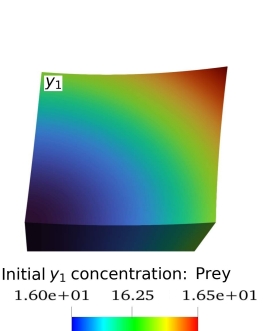
Figure 5.1. The $y_{1}(0,x_{1},x_{2})$ smooth initial data, while $y_{2}(0,x_{1},x_{2})=25$ everywhere in $\Omega$.

$y_{1}(0,x_{1},x_{2})={y_{1,0}}=16+0.25(x_{1}^{2}+x_{2}^{2})\,\text{ and }\,y_{2}(0,x)={y_{2,0}}=25{\text{ in }}\Omega,$ see Figure 5.1 for the prey initial concentration visualization, as well as, for some cases the nonsmooth/discontinuous initial conditions

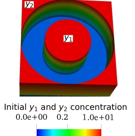
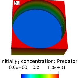
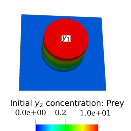
Figure 5.2. The $y_{1}(0,x_{1},x_{2})$ and $y_{2}(0,x_{1},x_{2})$ rough initial data.

(5.6) $$\begin{array}[]{l}y_{1,0}=\left\{{\begin{array}[]{*{20}{c}}{10,\quad{\rm{if}}{{(x_{1}-0.5)}^{2}}+{{(x_{2}-0.5)}^{2}}\leq\frac{1}{16}}\\ 1,\quad{\rm{otherwise}}\end{array}}\right.,\,\,y_{2,0}=\left\{{\begin{array}[]{*{20}{c}}{10,\quad{\rm{if}}{{(x_{1}-0.5)}^{2}}+{{(x_{2}-0.5)}^{2}}\geq\frac{1}{4}}\\ 1,\quad{\rm{otherwise}}\end{array}}\right.\end{array}$$

as seen in Figure 5.2, and with right hand forces

$$f_{1}=-(b\cos(t)\sin(t)\sin(\pi x)y^{2}sin(\pi y)+b\cos(t)\sin(t)x^{2}sin(\pi x)sin(\pi y)+64b\sin(t)sin(\pi x)sin(\pi y)$$

$$\qquad\,+\sin(t)y^{2}-25b\cos(t)y^{2}+64b\sin(t)sin(\pi x)sin(\pi y)+\sin(t)y^{2}-25b\cos(t)y^{2}+a\cos(t)y^{2}$$

$$\qquad\,+\sin(t)x^{2}-25b\cos(t)x^{2}+a\cos(t)x^{2}+4\epsilon_{1}\cos(t)-1600b+64a)/4,$$

$$f_{2}=(c\cos(t)\sin(t)\sin(\pi x)y^{2}\sin(\pi y)+c\cos(t)\sin(t)x^{2}\sin(\pi x)\sin(\pi y)+64c\sin(t)\sin(\pi x)\sin(\pi y)$$

$$\qquad-8\pi^{2}\epsilon_{1}\sin(t)\sin(\pi x)\sin(\pi y)-4d\sin(t)\sin(pi*x)\sin(\pi y)-4\cos(t)\sin(\pi x)\sin(\pi y)-25c\cos(t)y^{2}$$

$$\qquad\,-25c\cos(t)x^{2}-1600c+100d)/4.$$

Further, we enforce the target functions $(y_{1,d},y_{2,d})=(0,20)$ which physically means that we want the prey to vanish and the predator to dominate with a specific number. This makes sense e.g. in the case where the growth rate of $y_{1}$ is sluggish, the rate of $y_{2}$ killing $y_{1}$ is high, and the death rate of $y_{1}$ is high too with a sluggish death rate of $y_{2}$. We highlight that the uncontrolled system indicates that both species survive with such a cycle of survival as we will see later in the first snapshot of Figure 5.3, see also [33, p. 160], confirming the correctness of the target functions choice.
We assume the parameters $\epsilon_{1}=0.1$ (prey diffusion), $\epsilon_{2}=0.01$ (predator diffusion), $a=0.47$ (growth rate of prey), $b=0.024$ (searching efficiency/attack rate), $c=0.023$ (predator’s attack rate and efficiency at turning food into offspring-conversion efficiency), $d=0.76$ (predator mortality rate). The diffusion parameter values signify that the prey diffuses faster than the predator. The aforementioned parameter values were obtained from a related ordinary differential equation model for the classic Hudson Bay Company Hare-Lynx example.
The predator or the prey enters or exits in the domain $\Omega$ or the boundary $\Gamma$ in a controlled way, indicated by the distributed control or Robin boundary control functions $g_{i}$, $i=1,2$. Especially for the nonsmooth initial data case, the predator density at the starting point is concentrated near the corners of the domain, while the prey density is intensive around the center, see Figure 5.2. We note that the initial and boundary conditions may be difficult to pinpoint. Finally, we report that a nonlinear gradient method with strong Wolfe-Powel conditions and Fletcher-Reeves directions is employed for determining the optimal control functions. The values of $\gamma_{1}$, $\gamma_{2}$ have been tested in the interval $(10^{-1},10^{-5})$, and best selection approved to be $\gamma_{1}=\gamma_{2}=0.01$, see also [43, p. 218] and references therein.

5.1. Distributed control case.

This paragraph is dedicated to validating numerically that even if we force strict control constraints employing low order time polynomials –higher-order schemes are not applicable due to the irregularity that is caused by the control constraints– either unconstrained control for low and higher-order time polynomials, the results and the solutions’ distance from the target functions become efficiently small. In particular, we consider distributed control with and without control constraints, in cases with low and higher order time dG schemes respectively, and zero Dirichlet boundary conditions. Additionally, we report a qualitative study and the nullclines of the examined system.

5.1.1. Experiment A: control constraints $g_{ia}$, $g_{ib}$ and $k=0$, $l=1$.

We employ constant polynomials in time and linear in space. It is known that higher-order schemes are not applicable due to the irregularity that the control constraints cause to our system. We apply the control constraints $g_{ia}=0$ and $g_{ib}=0.1$. This choice is very strict considering that using the same data but with no control constraints we noticed that the control takes values in the interval $(0.9,3.55)$. The related results are demonstrated in Table 1 showing clearly that the state variables $y_{1}$, $y_{2}$ are driven efficiently to the desired targets $y_{1,d}$, $y_{2,d}$.

Table 1. Distributed control: Distance from the target for the 2d solution with $k=0$, $l=1$ ($\tau=\mathcal{O}(h^{2})$) with smooth data and control constraints.

Discretization	Distance from the target		Functional
$\tau=h^{2}/8$	${\left\|y_{1}-{y_{1,d}}\right\|}_{{L^{2}[0,T;{L}^{2}(\Omega)]}}$	$\left\|y_{2}-{y_{2,d}}\right\|_{{{L^{2}[0,T;{L}^{2}(\Omega)]}}}$	$J(y,g)$
$h=0.23570$	0.05672514712	0.031267953860	0.08799310282
$h=0.13888$	0.01417057646	0.004847915446	0.01901849221
$h=0.05892$	0.00354747615	0.000908289532	0.00445576574
$h=0.02946$	0.00088619624	0.000204350006	0.00109054626

It is worth noting that we take similar results if we implement the code for the same data but with no control constraints and using $k=0$, and $l=1$ polynomial degrees in time and in space respectively, although we omit these results for brevity.

5.1.2. Experiment B: unconstrained control and $k=1$, $l=2$.

In this experiment, in Table 2 the results for linear in time and quadratic in space polynomials have been reported. We note that the comparison of Table 1 ($k=0$, $l=1$) and Table 2 ($k=1$, $l=2$), indicate that it is not easy to further reduce significantly the functional even if we increase the order of polynomials in time and/or in space. We highlight that these difficulties appear in our opinion since the specific system consideration has to be controlled through both state variables $y_{1}$ and $y_{2}$, and the integration errors are accumulating especially in the cases of higher order dG in time, since e.g. for $k=1$ where the already quadruple optimal control system actually becomes eightfold. In our opinion, it is important though that the minimization functional is reduced even slightly. Similar behavior has been also depicted in the next Robin boundary related Experiment E after comparing Tables 3 ($k=0$, $l=1$), Table 4 ($k=1$, $l=1$) and Table 5 ($k=1$, $l=2$) in paqragraph 5.2.2, see also [14].

Table 2. Distributed control: Distance from the target for the 2d solution with $k=1$, $l=2$ ($\tau=\mathcal{O}(h^{2})$) with smooth data and without control constraints.

Discretization	Distance from the target		Functional
$\tau=h^{2}/8$	${\left\|y_{1}-{y_{1,d}}\right\|}_{{L^{2}[0,T;{L}^{2}(\Omega)]}}$	$\left\|y_{2}-{y_{2,d}}\right\|_{{{L^{2}[0,T;{L}^{2}(\Omega)]}}}$	$J(y,g)$
$h=0.23570$	0.05914777260	0.017063455880	0.076212590230
$h=0.13888$	0.01419612697	0.003323664495	0.017520155410
$h=0.05892$	0.00351236326	0.000785876982	0.004298333324
$h=0.02946$	0.00087479208	0.000195581819	0.001070397159

Concerning the distance between the state solution and the target function, we also notice that the predator concentration $y_{2}$ is driven closer to the target $y_{2,d}$ comparing it with the distance between $y_{1}$ and the target function $y_{1,d}$ and similar phenomenon we noticed for Experiment A. Also, It is observed that the lower-density starting meshes have good results for the $y_{1}$ state. This is natural since the prey diffusion $\epsilon_{1}=0.1$ is much bigger than the predator diffusion $\epsilon_{2}=0.01$. In order to achieve better results, an idea could be to use a multi-scaling approach, which would be investigated in future work.

5.1.3. Experiment C: Qualitative study and nullclines investigation.

For a deeper understanding of the solutions’ behavior, we demonstrate the system’s nullclines and the phase planes, which also exhibit the way the control functions affect the state solutions. Furthermore, the latter indicates the appropriate choice of parameters for the numerical simulation of optimal solutions. It is informative we add the phase planes of the system to a graph and essential to find the confined set and draw the nullclines of the system, that is, the curves in the phase plane (the curves on which one of the variables is stationary), see e.g. [48, p. 46-47,78] or [29]. In the following, we demonstrate a 4-step study to find the fixed points, the stability of the fixed points, the nodes, spirals, vortices, or possible saddles. Particularly, we name the nonlinear terms

$$\phi_{1}(y_{1},y_{2})=(a-by_{2})y_{1}$$

$$\phi_{2}(y_{1},y_{2})=(cy_{1}-d)y_{2},$$

and we follow the procedure as described in the next steps:

STEP 1: We solve the equations $\phi_{1}(y_{1},y_{2})=0$ and $\phi_{2}(y_{1},y_{2})=0$ and we see that the fixed points are $FP1=(0,0)$ and $FP2=(d/c,a/b)$.

STEP 2: For the fixed points stability, we examine the matrix

$$\Phi(y_{1},y_{2})=\left[\begin{array}[]{cc}\frac{\partial\phi_{1}}{\partial y_{1}}&\frac{\partial\phi_{1}}{\partial y_{2}}\\ \frac{\partial\phi_{2}}{\partial y_{1}}&\frac{\partial\phi_{2}}{\partial y_{2}}\\ \end{array}\right]=\left[\begin{array}[]{cc}a-by_{2}&-by_{1}\\ cy_{2}&cy_{1}-d\\ \end{array}\right],$$

with determinant ${\it\Delta}=(cy_{1}-d)(a-by_{2})+bcy_{1}y_{2}$ and trace $T=-by_{2}+cy_{1}-d+a$.

For $a=0.47$, $b=0.024$, $c=0.023$, $d=0.76$, we take for the $FP1$

$$\Phi(0,0)=\left[\begin{array}[]{cc}0.47&0\\ 0&-0.76\\ \end{array}\right],$$

and for the $FP2$

$$\Phi(d/c,a/b)=\Phi(33.043,19.583)=\left[\begin{array}[]{cc}0.0&-0.793\\ 0.450&-1.110\times 10^{-}16\\ \end{array}\right].$$

It is easy to see that the $FP2$ is a stable fixed point since the determinant of $\Phi(d/c,a/b)$ is positive and the trace of $\Phi(d/c,a/b)$ is negative, but $FP1$ is unstable.

STEP 3: In this step, we study the nature of the fixed points. Let $\it\Delta$ be the determinant of $\Phi$ and $T$ be the trace. The discriminant is

$$D = T^{2}-4{\it\Delta}$$

$$= b^{2}y_{2}^{2}+(-2bcy_{1}-2bd-2ab)y_{2}+c^{2}y_{1}^{2}$$

$$+(-2cd-2ac)y_{1}+d^{2}+2ad+a^{2}.$$

After some computations, we notice that the $FP2$ is a stable spiral fixed point since we observe two complex eigenvalues with negative real parts and occurs when $D<0$. Solutions spiral into that fixed point are depicted in Figure 5.3. Moreover, the $FP1$ is a saddle point since $\it\Delta<0$ and consists of one positive and one negative eigenvalue thus it is unstable.

Hence, in Figure 5.3,

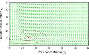
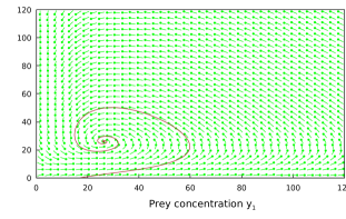
Figure 5.3. Phaseplanes for the $y_{1}(t,x,y)$ and $y_{2}(t,x,y)$ applying control $(g_{1},g_{2})=(0,0)$, $(0.1,0.1)$, $(1,1)$, $(1.5,1.5)$, $(2.5,2.5)$, $(4,4)$ and for parameters values: prey diffusion $\epsilon_{1}=0.1$, predator diffusion $\epsilon_{2}=0.01$, growth rate of prey $a=0.47$, searching efficiency/attack rate $b=0.024$, predator’s attack rate and efficiency at turning food into offspring-conversion efficiency $c=0.023$, predator mortality rate $d=0.76$.

we demonstrate the direction of the $(y_{1},y_{2})$ trajectory for control variable example values, and we draw the dynamics of the local kinetics for the point $(y_{1},y_{2})=(16.125,24)$, associated with the initial data for $(x_{1},x_{2})=(\frac{1}{2},\frac{1}{2})$, It is worth noting that we had similar trajectories for the test points $(y_{1},y_{2})=(16,25)$, $(16.125,24)$, $(16.25,25)$ and $(16.5,25)$.

The first visualization in Figure 5.3 corresponds to the uncontrolled case and is in agreement also to that in [41, p. 114]. Following the second to sixth visualization in the aforementioned figure, we demonstrate some examples of how the control affects the dynamics of the system.

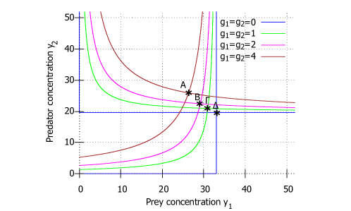
Figure 5.4. Nullclines for the $y_{1}(t,x,y)$ and $y_{2}(t,x,y)$ applying controls $(g_{1},g_{2})=(0,0)$, $(1,1)$, $(2,2)$, $(4,4)$ and for parameters: prey diffusion $\epsilon_{1}=0.1$, predator diffusion $\epsilon_{2}=0.01$, the growth rate of prey $a=0.47$, searching efficiency/attack rate $b=0.024$, predator’s attack rate and efficiency on turning food into offspring-conversion efficiency $c=0.023$, predator mortality rate $d=0.76$.

Figure 5.4 visualizes how the fixed point –an intersection of the nullclines for specific control values/intersection of lines with the same color– varies in some cases where we apply control. It also depicts how the control function changes the system’s dynamic. Moreover, the FP2 fixed point, from the initial value (without control) $(33.043,19.583)$ changes positions, namely to $(30.966,20.928)$, $(29.168,22.440)$, $(26.331,25.912)$ after applying some specific control values. Someone may also observe in the first column third snapshot, a typical example of how the control may drive the solution to the desired state $(0,20)$.

5.2. Boundary Robin control case.

Related to this model problem, we try to drive the solution to a desired target $({y_{1,d}},{y_{2,d}})$ minimizing the quadratic functional $J(y_{1},y_{2},g_{1},g_{2})$ described in (1.1) for $S=\Gamma$ subject to the constrains (1.4)-(1.5), and the initial conditions $y_{1}(0,x)={y_{1,0}}\quad y_{2}(0,x)={y_{2,0}}{\text{ in }}\Omega.$ Again, the state $y_{1}(t,x_{1},x_{2})$ represents the prey population density at time $t$ and $y_{2}(t,x_{1},x_{2})$ represents the predator population density both at time $t$ and position $(x_{1},x_{2})$. In the case of the Robin boundary control of the Lotka-Volterra system, numerical tests indicate that it is more difficult to achieve reliable numerical experimental results compared with the zero Dirichlet boundary conditions and distributed control. Similar issues have been noticed in [14, 13]. In our opinion, this is caused by the outwards normal derivative on the boundary, and even worse whether we apply boundary control. Subsequently, this phenomenon in the boundary affects also the solutions inside the domain and depends on the different diffusion properties. For the above reason, we need to use special tools for solving the optimal control problem. We employ the non-linear conjugate gradient methods for better results and best convergence properties and the Fletcher-Reeves directions together with the strong Wolfe-Powel conditions. These techniques have advantages such as being fast and with strong global convergence properties, [18], [21], but they also have some disadvantages that we will be concerned about in the following.

5.2.1. Experiment D: Constant in time ($k=0$), linear in space polynomials ($l=1$) and rough initial data.

In this example, we demonstrate the test case of the discontinuous initial conditions $y_{1}(0,x_{1},x_{2})$, $y_{2}(0,x_{1},x_{2})$ as they have been visualized in Figure 5.2. For the fully discrete scheme, we use constant in time polynomials combined with linear in space. This is an appropriate choice in cases with nonsmooth data, see e.g. [14]. We apply discontinuous initial data as in (5.6), for target functions $(y_{1,d},y_{2,d})=(0,20),$ that is the predator tends to dominate and the prey to vanish. We assume the parameters $\epsilon_{1}=0.1$, $\epsilon_{2}=0.01$, $a=0.47$, $b=0.024$, $c=0.023$, $d=0.76$ as in Experiments A, B, and for parameter values $\lambda_{1}=\lambda_{2}=1$, while our problem evolves in the time interval $[0,T]=[0,0.1]$ in a square $\Omega=[0,1]\times[0,1]$. The results reported in Table 3,

Table 3. Robin control: Distance from the target applying $k=0$, $l=1$ ($\tau=\mathcal{O}(h^{2})$) and rough data.

Discretization	Distance from the target		Functional
$\tau=h^{2}/2$	${\left\|y_{1}-{y_{1,d}}\right\|}_{{L^{2}[0,T;{L}^{2}(\Omega)]}}$	$\left\|y_{2}-{y_{2,d}}\right\|_{{{L^{2}[0,T;{L}^{2}(\Omega)]}}}$	$J(y,g)$
$h=0.23570$	0.04265266201	0.57806942650	0.6335395815
$h=0.13888$	0.00534571082	0.10386568510	0.1093306993
$h=0.05892$	0.00130612821	0.02562171016	0.0269393861
$h=0.02946$	0.00031866772	0.00648286241	0.0068040695

show that the manipulation is effective and the related distance size from the target may be reduced spectacularly. As expected, the control functions make the system more efficient as the time-space mesh becomes denser.

5.2.2. Experiment E: Linear in time ($k=1$), linear in space polynomials ($l=1$), smooth data.

We switch, and we introduce higher order polynomials in time, enforcing the smooth initial conditions $y_{1,0}=16+0.25(x_{1}^{2}+x_{2}^{2}),\,y_{2,0}=25$ and the same as the previous experiment’s target functions, considering Robin boundary control. The results are shown in i) Table 4 using linear in time and space polynomials and ii) for linear in time and quadratic in space in Table 5 for parameter values $\lambda_{1}=\lambda_{2}=1$.

Table 4. Robin control: Distance from the target applying $k=1$, $l=1$ ($\tau=\mathcal{O}(h^{2})$) and smooth data.

Discretization	Distance from the target		Functional
$\tau=h^{2}/2$	${\left\|y_{1}-{y_{1,d}}\right\|}_{{L^{2}[0,T;{L}^{2}(\Omega)]}}$	$\left\|y_{2}-{y_{2,d}}\right\|_{{{L^{2}[0,T;{L}^{2}(\Omega)]}}}$	$J(y,g)$
$h=0.23570$	0.4691621648	0.06976235262	0.5392965415
$h=0.13888$	0.0770592135	0.01100635051	0.1112083441
$h=0.05892$	0.0182574659	0.00242353097	0.0206912036
$h=0.02946$	0.0045402776	0.00057613379	0.0051184802

Table 5. Robin control: Distance from the target applying $k=1$, $l=2$ ($\tau=\mathcal{O}(h^{2})$) and smooth data.

Discretization	Distance from the target		Functional
$\tau=h^{2}/2$	${\left\|y_{1}-{y_{1,d}}\right\|}_{{L^{2}[0,T;{L}^{2}(\Omega)]}}$	$\left\|y_{2}-{y_{2,d}}\right\|_{{{L^{2}[0,T;{L}^{2}(\Omega)]}}}$	$J(y,g)$
$h=0.23570$	0.7186089436	0.06769868694	1.367070152
$h=0.13888$	0.0753016087	0.00951411931	0.084852089
$h=0.05892$	0.0182633483	0.00225891391	0.020530010
$h=0.02946$	0.0045402412	0.00056394557	0.005106144

This approach allows slightly better results regarding the distance from the target functions. We note that these boundary conditions restrict the regularity in the boundary, so it is strongly not recommended to employ higher-order polynomials in space even if we have a smooth initial data due to the limited regularity near the boundary caused by the Robin boundary conditions. The associated results are reported in Table 5. One also should expect that the experiment with $k=1$, $l=2$ would fail, and almost does in the coarse stepping mesh. Furthermore, the functional obviously has almost three times larger values than in the case with $k=1$, $l=1$ in Table 4 focusing on $h=0.23570$. Nevertheless, the parabolic regularity appears as the algorithm execution progresses and thus it is revealed beneficial.

In A, we introduce some basic aspects of the implementation and the algorithm we used.

5.3. Conclusion

We examined the Robin boundary and distributed control for a non-linear population model and we introduced the basic concepts of the first and second-order necessary conditions also in cases with control constraints. We demonstrated the related forward in time state and backward in time adjoint system, and a non-linear conjugate gradient method numerically verified that in each case we managed to manipulate the system to desired targets even in cases with rough initial data. We additionally demonstrated non-linear terms of the system qualitative analysis, extending and enriching the literature with the way that a control function changes the system’s quality, as well as, indicating the proper physical parameter value choices. We conclude that both the distributed and Robin boundary control for Lotka-Volterra system cases drive efficiently the state variables to desired targets. Nevertheless, the first case seems more stable and with a more robust minimization of the functional, fact justified from the lower regularity in the Robin boundary consideration. These minimization convergence issues in the second case motivated us to employ a non-linear gradient method while its implementation confirmed the aforementioned aspects. As future work, we are planning to extend and investigate in an optimal control framework state-of-the-art methods like the arbitrarily shaped finite element dG method [44], and/or unfitted mesh finite element methods possibly evolutionary in time and proper time discretization, [14, 46, 5, 6].

Appendix A Optimization procedure

The algorithm is based on the steepest–descent/projected gradient method combined with Strong Wolfe-Powel conditions and Fletcher-Reeves conjugate directions to ensure good convergence properties. Specifically, we consider the Fletcher-Reeves conjugate direction as the search direction to compute the step for this direction. The step $\epsilon_{n}$ is derived from a suitable linear search procedure. This approach makes us waste more computational resources in memory, but we can reduce significantly the number of iterations of the double iteration loop of the gradient method. We highlight that we noticed similar behavior with the results of a simple gradient method, but we gain faster convergence. Next, we introduce the strong Wolfe-Powel conditions with $0<\rho\leq\sigma<1$ and $d_{k+1}=-J^{\prime}_{k+1}+\beta_{k+1}d_{k}$, $d_{0}=-J^{\prime}_{k}$:

1. $J(y_{k+1},g_{k+1})\leq J(y_{k},g_{k})+\sigma\epsilon_{k}{J^{\prime T}}_{k}d_{k}$ (Armijo rule),

2. $|{J^{\prime}}_{k+1}d_{k}|\leq-\rho{J^{\prime}}_{k}d_{k}$,

with $0<\rho\leq\sigma<1$ and $d_{k+1}=-J^{\prime}_{k+1}+\beta_{k+1}d_{k}$, $d_{0}=-J^{\prime}_{k}$ and choosing the Fletcher-Reeves conjugate directions: $\beta_{k}=\frac{J^{\prime T}_{k}J^{\prime}_{k}}{\|J^{\prime}_{k-1}\|^{2}}$.
The pseudocode we used is:

Input: $n=0$, $\epsilon=1$, $tol=10^{-5}$, ${{g^{0}_{i}}}_{\Gamma}=1$, $y_{i}|_{t=0}$, $y_{id}$, $\sigma=0.1$, $\rho=0.9$,

Output: Optimal triple: $(y_{i},\mu_{i},{g_{i}}_{\Gamma})$

Solve: State problem for ${{{g^{0}_{i}}}_{\Gamma}}$

Compute $J^{0}$

%Main iteration

repeat

       Solve: Conjugate problem for $y^{n-1}_{i}$

       Compute $d^{0}_{i}=-J^{\prime 0}=-\gamma_{i}{g^{0}_{i}}_{\Gamma}+{\mu^{0}_{i}}_{\Gamma}$

       %Optimization iteration

       repeat

             %Fletcher–Reeves conjugate directions

             $\beta^{n}=\frac{{{J^{\prime}}^{n}}^{T}J^{\prime n}}{\|J^{\prime n-1}\|^{2}}$ %${J^{\prime}({g_{i}}_{\Gamma})}^{n}=\gamma_{i}{g^{n}_{i}}_{\Gamma}+{\mu^{n}_{i}}_{\Gamma}$

             $d^{n+1}_{i}=-J^{\prime n+1}+\beta^{n+1}_{i}d^{n}_{i}$

             ${g^{n}_{i}}_{\Gamma}={g^{n-1}_{i\,\,\Gamma}}+\epsilon d^{n+1}_{i}$

             Solve: State problem for ${g^{n}_{i}}_{\Gamma}$

             $\epsilon=0.5*\epsilon$

      until $|{{J^{\prime}}^{n+1}}^{T}d^{n}|>-\rho{{J^{\prime}}^{n}}^{T}d^{n}_{i}$

      if $|J^{n}-J^{n-1}|/J^{n}\leq tol$ then

             Break

       end if

      $\epsilon=1.5*\epsilon$

until $J(y^{n+1}_{i},{{g^{n+1}_{i\,\,\Gamma}}})>J(y^{n}_{i},{g^{n}_{i}}_{\Gamma})+\sigma\epsilon{{J^{\prime}}^{n}}^{T}d^{n}_{i}$ %Armijo rule

Optimization approach with preconditioned CG/nonlinear gradient method with strong Wolfe-Powel conditions and Fletcher-Reeves directions.

Where $i=1,2$ refers to the first and second species respectively and the projection step $\epsilon_{n}\equiv\epsilon$ is necessary since the direction term, it might not be admissible, see e.g. [35]. As we can see from the results in Tables 3, 4, 5 the algorithm is efficient and we can notice how the state solution distance from the target function for each variable and the quadratic functional reduces. Looking carefully at the results, the case with rough initial data is more demanding, while the quadratic functional values are larger in this case.

References

• [1] G. Akrivis, and M. Crouzeix, Linearly implicit methods for nonlinear parabolic equations. Math. Comp., 73, 613-635, 2004.
• [2] G. Akrivis, M. Crouzeix, and C. Makridakis, Implicit-explicit multistep finite element methods for nonlinear parabolic problems. Math. Comp., 67, 457-477, 1998.
• [3] G. Akrivis, and C. G. Makridakis, On maximal regularity estimates for discontinuous Galerkin time-discrete methods. SIAM. J. Numer. Anal., 60, 180–194, 2022.
• [4] G. Akrivis, and C. G. Makridakis, Galerkin time-stepping methods for nonlinear parabolic equations. ESAIM: Math. Model. and Numer. Anal., 38, 261–289, 2004.
• [5] A. Aretaki, and E. N. Karatzas, Random geometries for optimal control PDE problems based on fictitious domain FEMS and cut elements, Journal of Computational and Applied Mathematics, 412, 114-286, 2022.
• [6] A. Aretaki, E. N. Karatzas, and G. Katsouleas, Equal higher order analysis on an unfitted dG method for Stokes flow systems, Journal of Scientific Computing, 91(48), 2022.
• [7] J. F. Bonnans, Second Order Analysis for Control Constrained Optimal Control Problems of Semilinear Elliptic Systems. [Research Report] RR-3014 (Inria-00073680), INRIA. 1996.
• [8] A. Cagniani, E. H. Georgoulis, and M. Jensen, Discontinuous Galerkin methods for mass transfer through semi-permeable membranes. SIAM. J. Numer. Anal., 51, 2911– 2934, 2013.
• [9] H. Carreon, and F. Valdez, A New Optimization Method Based on the Lotka-Volterra System Equations. In: Castillo, O., Melin, P. (eds) New Perspectives on Hybrid Intelligent System Design based on Fuzzy Logic, Neural Networks and Metaheuristics. Studies in Computational Intelligence, vol 1050. Springer, Cham. 2022.
• [10] E. Casas, and K. Chrysafinos, A discontinuous Galerkin time stepping scheme for the velocity tracking problem, SIAM. J. Numer. Anal., 50 (2012), pp. 2281-2306.
• [11] P. Ciarlet, The finite element method for elliptic problems, SIAM Classics, Philadelphia, 2002.
• [12] K. Chrysafinos, and E. Karatzas, Symmetric error estimates for discontinuous Galerkin time-stepping schemes for optimal control problems constrained to evolutionary Stokes equations, Computational Optimization and Applications, 60(3), 719-751, 2015.
• [13] K. Chrysafinos, and E. Karatzas, Symmetric error estimates for discontinuous Galerkin approximations for an optimal control problem associated to semilinear parabolic PDEs, Disc. and Contin. Dynam. Syst. - Ser. B, 17, 1473 - 1506, 2012.
• [14] K. Chrysafinos, and E. Karatzas, Error Estimates for Discontinuous Galerkin Time-Stepping Schemes for Robin Boundary Control Problems Constrained to Parabolic PDEs, SIAM J. Numer. Anal., 52(6), 2837–2862, 2014.
• [15] K. Chrysafinos, E. Karatzas, and D. Kostas, Stability and error estimates of fully-discrete schemes for the Brusselator system, SIAM J. Numer. Anal., 57(2), 828–853, 2019.
• [16] K. Chrysafinos, and D. Kostas, Numerical Analysis of High Order Time Stepping Schemes for a Predator-Prey System, International Journal of Numerical Analysis and Modeling, 19(2-3), 404–423, 2022.
• [17] K. Chrysafinos, and D. Plaka, Analysis and approximations of an optimal control problem for the Allen–Cahn equation., Numer. Math., 155, 35-82, 2023.
• [18] Y. H. Dai, and Y. Yuan, A Nonlinear Conjugate Gradient Method with a Strong Global Convergence Property, SIAM J. Optim., 10(1), 177–182, 1999.
• [19] M. Delfour, W. Hager and F. Trochu, Discontinuous Galerkin Methods for Ordinary Differential Equations, Math. Comp, 36, 455-473, 1981.
• [20] F. Diele, M. Garvie, and C. Trenchea, Numerical analysis of a first-order in time implicit symplectic scheme for predator-prey systems, Comput. Math. Appl., 74, 948–961, 2017.
• [21] X. Dua, P. Zhang, and W. Ma, Some modified conjugate gradient methods for unconstrained optimization, Journal of Computational and Applied Mathematics, Volume 305, 92–114, 2016.
• [22] L. Evans, Partial Differential Equations, AMS, Providence RI, 1998.
• [23] K. Ericksson and C. Johnson, Adaptive finite element methods for parabolic problems IV: Nonlinear problems, SIAM J. Numer. Anal., 32, 1729-1749, 1995.
• [24] D. Estep and S. Larsson, The discontinuous Galerkin method for semilinear parabolic equations, RAIRO Model. Math. Anal. Numer., 27, 35-54, 1993.
• [25] M. Frittelli, A. Madzvamuse, I. Sgura, and C. Venkataraman, Lumped finite elements for reaction-cross-diffusion systems on stationary surfaces, Comput. Math. Appl., 74(12), 3008–3023, 2017.
• [26] J. L. GΓ‘mez, and J. A. C. Montero, Uniqueness of the optimal control for a Lotka-Volterra control problem with a large crowding effect, ESAIM: Control, Optimisation and Calculus of Variations, 2, 1-12, 1997.
• [27] H. Garcke, M. Hinze, and C. Kahle, Optimal control of time-discrete two-phase flow driven by a diffuse-interface model, ESAIM, Control Optim. Calc. Var., 25(13), 1-31, 2019.
• [28] M.R Garvie, and J.M. Blowey, A reaction-diffusion system of $\lambda$ $\omega$ type II: Numerical Analysis, Euro Jnl of Applied Mathematics, 16, 621–646, 2005.
• [29] M. Garvie, and C. Trenchea, Optimal Control of a Nutrient-Phytoplankton-Zooplankton-Fish System, SIAM J. Control Optim., 46(3), 775 - 791, 2007.
• [30] M. Garvie, and C. Trenchea, Finite element approximation of spatially extended predator interactions with the Holling type II functional response, Numer. Math., 107, 641–667, 2008.
• [31] M.D. Gunzburger and S. Manservisi, The velocity tracking problem for Navier–Stokes flow with boundary control, SIAM J. Control Optim., 39 , 594–634., 2000.
• [32] M.D. Gunzburger, L.S. Hou, and W. Zhu, Fully-discrete finite element approximation of the forced Fisher equation, J. Math. Anal. Appl., 313, 419-440, 2006.
• [33] A. Hastings, Population Biology, Springer, Berlin, Germany, 1997.
• [34] F. Hecht, New development in FreeFem++, Journal of numerical mathematics, 20(3-4), 251–265, 2012.
• [35] R. Herzog, and K. Kunisch, Algorithms for PDE-constrained optimization, GAMM-Mitteilungen, 33(2), 163–176, 2010.
• [36] R. C.S. Holling, Some characteristics of simple types of predation and parasitism, Can. Entomol., 91, 163–176, 385- 398.
• [37] C.S. Holling, The functional response of predators to prey density and its role in mimicry and population regulation, Mem. Entomol. Soc. Can., 45, 1-60, 1965.
• [38] M. HoltmannspΓΆtter and A. RΓΆsch, A priori error estimates for the finite element approximation of a nonsmooth optimal control problem governed by a coupled semilinear PDE-ODE system, SIAM J. Control Optim., 5, 3329-3358, 2021.
• [39] A. Ibanez, Optimal control of the Lotka–Volterra system: turnpike property and numerical simulations, Journal of Biological Dynamics, 11:1, 25-41, 2017.
• [40] D. Jackson, Error estimates for the semidiscrete Galerkin approximations of the FitzHugh-Nagumo equations, Appl. Math. Comput., 50, 93–114, 1992.
• [41] D.S. Jones, Michael Plank, and B.D. Sleeman, Differential Equations and Mathematical Biology, CHAPMAN & HALL/CRC, Second Edition, 2009.
• [42] L. Ju, X. Li, Z. Qiao, and H. Zhang, Energy stability and error estimates of exponential time differencing schemes for the epitaxial growth model without slope selection, Math. of Comput., 87, 1859–1885, 2018.
• [43] E. N. Karatzas, Optimal Control and Parabolic Problems, Numerical Analysis and Applications, http://dx.doi.org/10.26240/heal.ntua.1496, 2015.
• [44] E. N. Karatzas, hp-version analysis for arbitrarily shaped elements on the boundary discontinuous Galerkin method for Stokes systems, under revision, arXiv:2301.12577, 2024.
• [45] E. N. Karatzas, and G. Rozza, A Reduced Order Model for a Stable Embedded Boundary Parametrized Cahn–Hilliard Phase-Field System Based on Cut Finite Elements, J Sci Comput, 89(9), 2021.
• [46] G. Katsouleas, E. N. Karatzas, and F. Travlopanos, Discrete Empirical Interpolation and unfitted mesh FEMs: application in PDE–constrained optimization, Optimization Journal, 72(6), 1609–1642, 2023.
• [47] Z. Lin, R. Ruiz-Baier, and C. Tian, Finite volume element approximation of an inhomogeneous Brusselator model with cross-diffusion, Journal of Comput. Phys., 256, 806–823, 2014.
• [48] J.D. Murray, Mathematical Biology II: Spatial Models and Biomedical Applications, Third Edition, Springer, 2003.
• [49] I. Neitzel, and B. Vexler, A priori error estimates for space-time finite element discretization of semilinear parabolic optimal control problems, Numer. Math., 120, 345-386, 2012.
• [50] J. F. Rosenblueth, and G. S. Licea, Cones of critical directions in optimal control, Int. J. Med. Eng. Informat., 7, 55-67, 2013.
• [51] S. Ruuth, Implicit-explicit methods for reaction-diffusion problems in pattern-formation, J. Math. Biol., 34, 148-176, 1995.
• [52] F. TrΓΆltzsch, Optimal control of partial differential equations: Theory, methods and applications, Graduate Studies in Mathematics, AMS, 112, Providence 2010.
• [53] F. TrΓΆltzsch, E. Casas, and J. C. de los Reyes, Sufficient Second-Order Optimality Conditions for Semilinear Control Problems with Pointwise State Constraints, SIAM Journal on Optimization, 19(2), 2008, 616-643.
• [54] V. Volterra, Variations and fluctuations in the numbers of coexist Theoretical Ecology: 1923-1940, (Eds. F.M. Scudo and J.R. Ziegler), Lecture Notes in Biomathematics, Vol. 22, 65-236, Springer, Berlin, Heidelberg, 1978.