Topology of Discrete Quantum Feedback Control

Abstract

A general framework for analyzing topology of quantum channels of single-particle systems is developed to find a class of genuinely dynamical topological phases that can be realized by means of discrete quantum feedback control. We provide a symmetry classification of quantum channels by identifying ten symmetry classes of discrete quantum feedback control with projective measurements. We construct various types of topological feedback control by using topological Maxwell’s demons that achieve robust feedback-controlled chiral or helical transport against noise and decoherence. Topological feedback control thus offers a versatile tool for creating and controlling nonequilibrium topological phases in open quantum systems that are distinct from non-Hermitian and Lindbladian systems and should provide a guiding principle for topology-based design of quantum feedback control.

I Introduction

Topology plays a key role in classification and characterization of diverse physical phenomena that are robust against local disturbances. In particular, topological phases of matter have been discussed in a wide variety of quantum and classical systems, which are characterized by global geometric structures of eigenstates rather than local order parameters [1, 2, 3, 4, 5, 6]. A quintessential example of topological quantum phenomena is the quantum Hall effect, where chiral transport immune to disorder emerges along the edges of a system [7, 8, 9, 10, 11]. Furthermore, topological phases are enriched by symmetry. For example, time-reversal symmetry permits helical edge states, where time-reversal partners flow in opposite directions with no net mass current which is known as the quantum spin Hall effect [12, 13, 14, 15, 16]. Classification of phases of matter through integration of topology and symmetry has been of central interest in condensed matter physics [17, 18, 19].

The general concept of topology can also be utilized to classify nonequilibrium dynamics. Examples include periodically driven (Floquet) systems characterized by topology of unitary time-evolution operators [20, 21, 22, 23, 24, 25, 26, 27, 28, 29, 30, 31] and topological phases of open systems described by non-Hermitian Hamiltonians [32, 33, 34, 35, 36, 37, 38]. Notably, out-of-equilibrium driving not only provides a useful tool for controlling topological phases, but also induces genuinely dynamical topological phases that has no static counterpart [22, 39, 28, 33]. Finding a new control method for topological phases thus expands the scope of research of topological phases of matter.

Feedback control provides a versatile tool for a wide range of applications in science and technology [40]. In particular, in the research arena of high-precision measurement and control of quantum systems, feedback control has achieved suppression of quantum noise [41], stabilization of desired states [42, 43], cooling [44, 45, 46], and quantum error correction [47, 48, 49, 50]. Feedback control also allows operations that would otherwise be impossible. An illustrative example is Maxwell’s demon, which was originally conceived as an intelligent being that can decrease entropy of a system against the second law of thermodynamics [51]. In modern language, Maxwell’s demon can be formulated as a feedback controller [52, 53], and various types of Maxwell’s demon have experimentally been realized in both classical [54, 55, 56, 57] and quantum [58, 59, 60, 61, 62, 63] systems. In view of versatile applicability of feedback control, we are naturally led to the following question: can we utilize feedback control to create and manipulate nonequilibrium topological phases? This is the problem we wish to address in this paper.

In this paper, we present a class of dynamical topological phases that can be realized with feedback control of quantum systems. Here, a unique role played by feedback control is that one can choose operations in such a manner that they depend on measurement outcomes. This flexibility enables versatile real-time control of topological phases that would be hard to achieve by unitary dynamics in which the driving protocol is predetermined and cannot depend on the state of a system under control. Furthermore, feedback control enables active control of a quantum system, in contrast with passive control of open quantum systems by engineered dissipation.

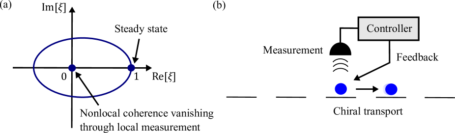
Figure 1: (a) Schematic illustration of the eigenspectrum (shown by a blue curve and two blue dots) of a quantum channel for topological quantum feedback control. The spectrum involves a closed loop characterized by a winding number and highly degenerate zero eigenvalues due to local measurement through which nonlocal coherence vanishes. The unit eigenvalue corresponds to a steady state. (b) Discrete quantum feedback control is comprised of a quantum measurement and a subsequent operation depending on the measurement outcome. Topologically nontrivial winding of the eigenspectrum of a quantum channel [see (a)] implies chiral (unidirectional) transport of a particle on a lattice due to feedback control.

Table 1: Comparison of different classes topological phases. The first row shows five classes of topological phases characterized by the topology of relevant operators which are shown in the second row. The third row indicates whether the dynamics is discrete or continuous. The fourth row shows whether the system is closed or open. The fifth row shows whether a quantum state is pure or mixed.

Class	Ground state	Floquet	Non-Hermitian	Lindblad	Discrete quantum feedback
Operator	Hamiltonian	Unitary	Non-Hermitian Hamiltonian	Lindbladian	Quantum channel
Time evolution	Static	Discrete	Continuous	Continuous	Discrete
Closed/open	Closed	Closed	Open	Open	Open
Pure/mixed	Pure	Pure	Pure	Mixed	Mixed

We develop a general framework for analyzing topology of quantum channels for discrete quantum feedback control. Mathematically, quantum channels are described by completely positive and trace-preserving (CPTP) maps, which provide a general form of time evolution in open quantum systems [47]. Here, the time evolution of a system under feedback control is nonunitary due to measurement backaction. Consequently, topology of CPTP maps is intrinsically non-Hermitian and beyond the theoretical framework of static (Hermitian) topological phases. We introduce topological invariants of quantum channels for single-particle systems on lattices under the general assumption of locality in measurement and feedback. For example, a nonzero winding number of the eigenspectrum of a quantum channel implies chiral transport due to feedback control, which may be regarded as a feedback-controlled counterpart of chiral edge transport in quantum Hall systems as schematically illustrated in Fig. 1.

Quantum feedback control creates a class of nonequilibrium open quantum systems distinct from those described by non-Hermitian Hamiltonians [33, 34, 35] and Lindblad master equations [64, 65, 66, 67]. We summarize the comparison of different classes of topological phases in Table 1. In particular, discrete quantum feedback control concerns discrete time evolution from an initial quantum state to a post-feedback quantum state. Such time evolution cannot in general be expressed by using a generator of continuous time evolution. In fact, as shown in Sec. III, CPTP maps with local Kraus operators have highly degenerate zero eigenvalue, and therefore cannot be described by using any generator [see Eq. (39)]. Physically, the existence of zero eigenvalues can be understood as a consequence of local measurement through which nonlocal coherence in an extended system vanishes [see Fig. 1(a) and Sec. III]. A non-Hermitian Hamiltonian can only describe the dynamics of pure states and thus requires postselection of particular measurement outcomes [68]. The Lindblad quantum master equation describes the dynamics of mixed states but does not refer to measurement outcomes [40]. In contrast, nonequilibrium topological phases created by quantum feedback control are realized by a nontrivial interplay between quantum measurement and feedback operations. We note that non-Hermitian topology has been applied to quantum channels in Ref. [33]. However, its application beyond zero-dimensional systems is nontrivial; in fact, the locality of Kraus operators is the key for defining topological invariants, as discussed in Sec. III.

We present prototypical models of topological feedback control by using quantum Maxwell’s demons, which we shall refer to as topological Maxwell’s demons. In a one-dimensional case, a topological Maxwell’s demon causes feedback-assisted chiral transport due to topology. We find that the topological Maxwell’s demon can generate topologically distinct phases by changing the duration of feedback control. We also show that feedback control can induce the non-Hermitian skin effect, which is a hallmark of dynamical topology unique to open systems [69, 70, 33, 71, 72, 73, 38, 74]. The chiral transport caused by the topological Maxwell’s demon is protected by topology and hence robust against noise and decoherence during the feedback process.

Symmetry plays a pivotal role in classification of topological phases [18, 17, 19, 27, 28, 33, 34, 35, 65, 37, 66, 67]. Here, we perform a symmetry classification of quantum feedback control. We find that only a subset of the 38 symmetry classes of non-Hermitian matrices [75, 34, 35] is compatible with quantum channels with projective measurements. We identify ten relevant symmetry classes of quantum channels for discrete quantum feedback control (see Table 2), and provide examples of feedback control for each class. In particular, we propose a quantum Maxwell’s demon with a two-point measurement as an example of symmetry-protected topological feedback control. This demon generates helical spin transport protected by symmetry, which may be regarded as a counterpart of the quantum spin Hall effect in feedback-controlled quantum systems.

Table 2: Ten-fold symmetry classification of discrete quantum feedback control with projective measurement. Each symmetry class is defined according to the presence or absence of $C,K$, and $Q$ symmetries in the CPTP map. Here, $C,K$, and $Q$ symmetries of a CPTP map $\mathcal{E}$ are defined by $\mathcal{V}_{C}\mathcal{E}^{T}\mathcal{V}_{C}^{-1}=\mathcal{E},\mathcal{V}_{K}\mathcal{E}^{*}\mathcal{V}_{K}^{-1}=\mathcal{E}$, and $\mathcal{V}_{Q}\mathcal{E}^{\dagger}\mathcal{V}_{Q}^{-1}=\mathcal{E}$, respectively, where $\mathcal{V}_{X}$ ($X=C,K,Q$) is a unitary superoperator. In the Table, $0$ indicates the absence of symmetry, and $\pm 1$ indicates the presence of symmetry with $\mathcal{V}_{X}\mathcal{V}_{X}^{*}=\pm\mathcal{I}$, where $\mathcal{I}$ denotes the identity superoperator. The labeling of the symmetry classes follows Ref. [34], where psH denotes pseudo-Hermiticity and the subscript $+$ ($-$) of psH indicates that the unitary superoperator for $C$ or $K$ symmetry commutes (anticommutes) with that of the pseudo-Hermiticity. In addition to the symmetry classes of a CPTP map $\mathcal{E}$, the corresponding Altland-Zirnbauer^† classes of $i\mathcal{E}$ are shown in the parentheses. In the fifth column, examples of conditions for feedback (FB) control in each symmetry class are shown (see Sec. VI for detailed discussions). CPTP maps with $C$ or $Q$ symmetry can be realized with feedback control with a two-point measurement (2PM). Symmetry classes without $K$ symmetry with $\mathcal{V}_{K}\mathcal{V}_{K}^{*}=+\mathcal{I}$ require unitary symmetry (US) due to the intrinsic modular conjugation symmetry of CPTP maps. AUS_- denotes antiunitary symmetry whose square gives $-1$. Some symmetry classes may be realized with an additional feedback control that enforces the symmetry condition (see examples in Sec. VII). The rightmost column shows concrete models of topological feedback control, which are presented in Sec. IV and Sec. VII.

Class	$C$	$K$	$Q$	Example of conditions	Model
A	$0$	$0$	$0$	US	QND demon
psH (AIII)	$0$	$0$	$1$	US, 2PM, and modified reciprocity
AI†	$+1$	$0$	$0$	US, 2PM, and reciprocity
AI$+$psH+ (BDI†)	$+1$	$+1$	$1$	2PM and reciprocity
AI (D†)	$0$	$+1$	$0$	No symmetry or particle-hole symmetry	Chiral Maxwell’s demon / SSH demon
AI$+$psH- (DIII†)	$-1$	$+1$	$1$	2PM, reciprocity, and additional FB	Helical Maxwell’s demon
AII†	$-1$	$0$	$0$	US, 2PM, reciprocity, and additional FB	$\mathbb{Z}_{2}$ demon
AII$+$psH+ (CII${}^{\dagger})$	$-1$	$-1$	$1$	US, 2PM, AUS-, reciprocity, and additional FB
AII (C†)	$0$	$-1$	$0$	US and AUS-
AII$+$psH- (CI†)	$+1$	$-1$	$1$	US, 2PM, AUS-, and reciprocity

The rest of this paper is organized as follows. In Sec. II, we introduce quantum channels that describe discrete quantum feedback control. In Sec. III, we use the Bloch theory of translationally invariant quantum channels to show that topological invariants of quantum channels can be defined when Kraus operators are local in space. In Sec. IV, we construct an example of topological feedback control, which shows feedback-induced chiral transport due to its point-gap topology. In Sec. V, we examine symmetry of discrete quantum feedback control and identify ten symmetry classes that are compatible with projective measurement. We also discuss how to construct feedback control in each symmetry class in Sec. VI. On the basis of the symmetry classification, we provide various models of symmetry-protected topological feedback control in Sec. VII. In particular, we present topological feedback control protected by transposition symmetry which exhibits helical spin transport due to an interplay between symmetry and topology. In Sec. VIII, we extend our theory to the case of nonunitary feedback control, thereby showing robustness of topological feedback control against dissipation. We also propose feedback control with engineered dissipation, where dissipation is used as an essential tool to achieve feedback control. We conclude this paper in Sec. IX with an outlook. In Appendix A, we present the detail of the Bloch theory of quantum channels. In Appendix B, we describe the Bloch theory of quantum feedback control with projective measurement. In Appendix C, we discuss a spectral property of quantum channels for projective measurement. In Appendix D, we summarize the correspondence between symmetry of time-evolution operators and that of their generators. In Appendix E, we present a supplementary discussion of symmetry-preserving boundary conditions for a $\mathbb{Z}_{2}$ Maxwell’s demon.

II Discrete quantum feedback control

We consider discrete quantum feedback control in which a feedback cycle consists of quantum measurements and subsequent unitary operations that are conditioned on measurement outcomes. Let $\hat{\rho}_{\mathrm{i}}$ be the initial density matrix of a system. We first perform a quantum measurement described by a set of measurement operators $\{\hat{M}_{m}\}$ subject to

$$\sum_{m}\hat{M}_{m}^{\dagger}\hat{M}_{m}=\hat{I},$$ (1)

where the index $m$ specifies a measurement outcome and $\hat{I}$ is the identity operator [40]. The probability of an outcome $m$ is given by $p_{m}=\mathrm{Tr}[\hat{M}_{m}^{\dagger}\hat{M}_{m}\hat{\rho}_{\mathrm{i}}]$, and the postmeasurement state corresponding to an outcome $m$ is given by

$$\hat{\rho}_{m}=\frac{\hat{M}_{m}\hat{\rho}_{\mathrm{i}}\hat{M}_{m}^{\dagger}}{p_{m}},$$ (2)

where the nonunitary state change is caused by measurement backaction. Then, we let the system undergo unitary time evolution during time $\tau$, which is described by a unitary operator

$$\hat{U}_{m}=\mathcal{T}\exp\Bigl{[}-i\int_{0}^{\tau}dt\hat{H}_{m}(t)\Bigr{]},$$ (3)

where $\hat{H}_{m}(t)$ is the feedback Hamiltonian which depends on the measurement outcome $m$ and $\mathcal{T}$ is the time-ordering operator. We set $\hbar=1$ throughout this paper. If we take an ensemble average over measurement outcomes, the final density matrix after one feedback loop is given by [52]

$$\hat{\rho}_{\mathrm{f}}= \sum_{m}p_{m}\hat{\rho}^{\prime}_{m}$$

$$= \sum_{m}\hat{U}_{m}\hat{M}_{m}\hat{\rho}_{\mathrm{i}}\hat{M}_{m}^{\dagger}\hat{U}_{m}^{\dagger},$$ (4)

where $\hat{\rho}^{\prime}_{m}=\hat{U}_{m}\hat{\rho}_{m}\hat{U}_{m}^{\dagger}$ is the density matrix after feedback control with measurement outcome $m$. Thus, a discrete quantum feedback control is described by a quantum channel

$$\mathcal{E}(\hat{\rho}):= \sum_{m}\hat{U}_{m}\hat{M}_{m}\hat{\rho}\hat{M}_{m}^{\dagger}\hat{U}_{m}^{\dagger}$$

$$= \sum_{m}\hat{K}_{m}\hat{\rho}\hat{K}_{m}^{\dagger},$$ (5)

which is a completely positive and trace-preserving (CPTP) map [47], where $\hat{K}_{m}:=\hat{U}_{m}\hat{M}_{m}$ is the Kraus operator satisfying $\sum_{m}\hat{K}_{m}^{\dagger}\hat{K}_{m}=\hat{I}$.

If a feedback cycle is repeated, the final density matrix is given by applying CPTP maps multiple times. Suppose that we repeat a measurement and a feedback operation $N$ times. Let $(m_{1},m_{2},\cdots,m_{N})$ be a sequence of measurement outcomes through this process. After the $n$th measurement, we perform a feedback operation as

$$\hat{\rho}_{m_{1},\cdots,m_{n}}^{\prime}=\hat{U}_{m_{n}}\hat{\rho}_{m_{1},\cdots,m_{n}}\hat{U}_{m_{n}}^{\dagger},$$ (6)

where

$$\hat{\rho}_{m_{1},\cdots,m_{n}}=\frac{\hat{M}_{m_{n}}\hat{\rho}_{m_{1},\cdots,m_{n-1}}^{\prime}\hat{M}_{m_{n}}^{\dagger}}{p(m_{n}|m_{1},\cdots,m_{n-1})}$$ (7)

is the density matrix after the $n$th measurement and

$$p(m_{n}|m_{1},\cdots,m_{n-1})=\mathrm{Tr}[\hat{M}_{m_{n}}^{\dagger}\hat{M}_{m_{n}}\hat{\rho}_{m_{1},\cdots,m_{n-1}}^{\prime}]$$ (8)

is the probability of an outcome $m_{n}$, conditioned on the past outcomes $m_{1},\cdots,m_{n-1}$. Then, the final density matrix $\hat{\rho}_{\mathrm{f}}^{(N)}$ averaged over all measurement outcomes is given by

$$\hat{\rho}_{\mathrm{f}}^{(N)}= \sum_{m_{1},\cdots,m_{N}}p(m_{N}|m_{1},\cdots,m_{N-1})p(m_{N-1}|m_{1},\cdots,m_{N-2})\cdots p(m_{2}|m_{1})p_{m_{1}}\hat{\rho}_{m_{1},\cdots,m_{N}}^{\prime}$$

$$= \sum_{m_{1},\cdots,m_{N}}\hat{U}_{m_{N}}\hat{M}_{m_{N}}\cdots\hat{U}_{m_{1}}\hat{M}_{m_{1}}\hat{\rho}_{\mathrm{i}}\hat{M}_{m_{1}}^{\dagger}\hat{U}_{m_{1}}^{\dagger}\cdots\hat{M}_{m_{N}}^{\dagger}\hat{U}_{m_{N}}^{\dagger}$$

$$= \mathcal{E}^{N}(\hat{\rho_{\mathrm{i}}}).$$ (9)

Thus, repeated feedback control is described by the repeated application of a CPTP map. Equation (9) suggests an analogy between periodically driven (Floquet) quantum systems [21, 22, 23, 24, 25, 26, 27, 28, 29, 30, 31] and feedback-controlled quantum systems: a unitary time-evolution operator for one period is repeatedly applied to a state vector in the former, while a CPTP map is repeatedly applied to a density matrix in the latter (see also Table 1).

The above description can be generalized to the cases in which different measurement and feedback operations are performed multiple times during a single cycle. For example, let us perform a second measurement with measurement operators $\{\hat{M}_{m_{2}}^{\prime}\}$ after the first measurement and the subsequent feedback operation. Then, we perform the second feedback control with unitary operators $\{\hat{U}_{m_{1},m_{2}}^{\prime}\}$, which may depend on the outcomes of the first and second measurements. The overall feedback cycle is described by a CPTP map

$$\mathcal{E}^{\prime}(\hat{\rho})= \sum_{m_{1},m_{2}}\hat{K}_{m_{1},m_{2}}^{\prime}\hat{\rho}(\hat{K}_{m_{1},m_{2}}^{\prime})^{\dagger},$$ (10)

where $\hat{K}_{m_{1},m_{2}}^{\prime}=U_{m_{1},m_{2}}^{\prime}\hat{M}_{m_{2}}^{\prime}\hat{U}_{m_{1}}\hat{M}_{m_{1}}$ is the Kraus operator. More general cases with nonunitary feedback operations will be discussed in Sec. VIII.

Let $\mathcal{H}$ be a finite-dimensional Hilbert space of the system. Then, the density matrix $\hat{\rho}$ is an element of the space $\mathcal{L}(\mathcal{H})$ of linear operators on $\mathcal{H}$, which is a Hilbert space with dimension $(\dim\mathcal{H})^{2}$. The Hilbert-Schmidt inner product in $\mathcal{L}(\mathcal{H})$ is denoted by $\langle\hat{A},\hat{B}\rangle:=\mathrm{Tr}[\hat{A}^{\dagger}\hat{B}]$. A CPTP map $\mathcal{E}$ [Eq. (5)] is regarded as an operator acting on the operator space $\mathcal{L}(\mathcal{H})$ (i.e., $\mathcal{E}$ is a superoperator). The adjoint superoperator $\mathcal{E}^{\dagger}$ is defined by

$$\mathcal{E}^{\dagger}(\hat{\sigma}):=\sum_{m}\hat{K}_{m}^{\dagger}\hat{\sigma}\hat{K}_{m},$$ (11)

which satisfies $\langle\hat{\sigma},\mathcal{E}(\hat{\rho})\rangle=\langle\mathcal{E}^{\dagger}(\hat{\sigma}),\hat{\rho}\rangle$.

We consider the eigenvalue problem of a CPTP map for feedback control:

$$\mathcal{E}(\hat{\rho}_{n}^{R})=\xi_{n}\hat{\rho}_{n}^{R},$$ (12)

$$\mathcal{E}^{\dagger}(\hat{\rho}_{n}^{L})=\xi_{n}^{*}\hat{\rho}_{n}^{L},$$ (13)

where $\xi_{n}\in\mathbb{C}$ denotes an eigenvalue and $\hat{\rho}_{n}^{R}$ ($\hat{\rho}_{n}^{L}$) is the corresponding right (left) eigenoperator which satisfies the biorthogonal condition $\mathrm{Tr}[(\hat{\rho}_{m}^{L})^{\dagger}\hat{\rho}_{n}^{R}]=0$ for $m\neq n$. By using the eigensystem of the CPTP map $\mathcal{E}$, the density matrix after a feedback loop in Eq. (4) is expanded as

$$\hat{\rho}_{\mathrm{f}}=\mathcal{E}(\hat{\rho}_{\mathrm{i}})=\sum_{n}c_{n}\xi_{n}\hat{\rho}_{n}^{R},$$ (14)

where

$$c_{n}= \frac{\langle\hat{\rho}_{n}^{L},\hat{\rho}_{\mathrm{i}}\rangle}{\langle\hat{\rho}_{n}^{L},\hat{\rho}_{n}^{R}\rangle}$$ (15)

is an expansion coefficient which depends on the initial state $\hat{\rho}_{\mathrm{i}}$. Here, for simplicity we assume that the CPTP map is diagonalizable. If the CPTP map is not diagonalizable, we can expand the density matrix by using generalized eigenmodes [68]. Thus, the eigenvalues and the (generalized) eigenmodes of the CPTP map completely characterize the discrete quantum feedback control.

An eigensystem of a CPTP map has some general properties (see Fig. 1(a) for a schematic illustration). First, all the eigenvalues $\xi_{n}$ of a CPTP map satisfies $|\xi_{n}|\leq 1$ because of the contraction property of a CPTP map [76]. An eigenmode $\hat{\rho}_{\mathrm{SS}}$ with eigenvalue $+1$ is a steady state of the dynamics in the sense that $\mathcal{E}(\hat{\rho}_{\mathrm{SS}})=\hat{\rho}_{\mathrm{SS}}$. Second, since a CPTP map preserves the trace of the density matrix, that is, $\mathrm{Tr}[\mathcal{E}(\hat{\rho})]=\mathrm{Tr}[\hat{\rho}]$, all the right eigenmodes except for those corresponding to steady states are traceless: $\mathrm{Tr}[\hat{\rho}_{n}^{R}]=0\ (\xi_{n}\neq 1)$. Third, a CPTP map preserves the Hermiticity of an operator since

$$[\mathcal{E}(\hat{\rho})]^{\dagger}=\mathcal{E}(\hat{\rho}^{\dagger}).$$ (16)

It follows from Eqs. (12) and (16) that if $\hat{\rho}_{n}^{R}$ is an eigenmode of $\mathcal{E}$ with eigenvalue $\xi_{n}$, then $(\hat{\rho}_{n}^{R})^{\dagger}$ is also an eigenmode with eigenvalue $\xi_{n}^{*}$ since

$$\mathcal{E}((\hat{\rho}_{n}^{R})^{\dagger})=[\mathcal{E}(\hat{\rho}_{n}^{R})]^{\dagger}=\xi_{n}^{*}(\hat{\rho}_{n}^{R})^{\dagger}.$$ (17)

Therefore, eigenvalues of a CPTP map are real or appear as complex-conjugate pairs.

III Topological equivalence of quantum channels

In this section, we introduce topology of quantum channels (CPTP maps) to investigate topological phases induced by feedback control.

III.1 Setup

We consider discrete quantum feedback control of a single-particle quantum system on a $d$-dimensional lattice. Let

$$\Lambda:=\{\vec{R}_{\vec{i}}=\sum_{\lambda=1}^{d}i_{\lambda}\vec{a}_{\lambda};\ \vec{i}=(i_{1},\cdots,i_{d}),i_{\lambda}=0,\cdots,L_{\lambda}-1\}$$ (18)

be a set of lattice sites, where $\vec{a}_{\lambda}\ (\lambda=1,\cdots,d)$ denote the primitive lattice vectors. Each lattice site $\vec{R}_{\vec{i}}$ is specified by a set of integers $\vec{i}=(i_{1},\cdots,i_{d})$. The total number of unit cells is given by $N_{\mathrm{cell}}:=L_{1}L_{2}\cdots L_{d}$. The Hilbert space of the system is spanned by a basis $\{\ket{\vec{i},a}\}$ ($\vec{i}=(i_{1},\cdots,i_{d}),i_{\lambda}=0,\cdots,L_{\lambda}-1$, and $a=1,\cdots,D_{\mathrm{loc}}$), where $\ket{\vec{i},a}$ denotes the quantum state at site $\vec{i}$, and the index $a$ labels additional degrees of freedom such as spin, orbit, sublattice, etc. The dimension of the Hilbert space in each unit cell is denoted by $D_{\mathrm{loc}}$, and thus the dimension of the entire Hilbert space $\mathcal{H}$ of the system is given by $D=N_{\mathrm{cell}}D_{\mathrm{loc}}$. (Note that we consider a one-body problem here.) The density matrix of the system can be expanded in terms of the orthonormal basis as

$$\hat{\rho}=\sum_{\vec{i},\vec{j}}\sum_{a,b}\rho_{\vec{i},a;\vec{j},b}\ket{\vec{i},a}\bra{\vec{j},b}.$$ (19)

We impose the periodic boundary condition

$$\ket{\vec{i}+L_{\lambda}\vec{e}_{\lambda},a}=\ket{\vec{i},a}\ (\lambda=1,\cdots,d),$$ (20)

where $\vec{e}_{\lambda}$ is a unit vector defined by $(\vec{e}_{\lambda})_{\lambda^{\prime}}=\delta_{\lambda,\lambda^{\prime}}$, unless otherwise specified.

We perform feedback control of the system with a CPTP map (5). We assume that the Kraus operators $\hat{K}_{m}$ do not change the particle number of the system. The Kraus operators are expanded by using the orthonormal basis as

$$\hat{K}_{m}=\sum_{\vec{i},\vec{j}}\sum_{a,b}(\hat{K}_{m})_{\vec{i},a;\vec{j},b}\ket{\vec{i},a}\bra{\vec{j},b}.$$ (21)

Since a CPTP map is a superoperator acting on the operator space, it is convenient to vectorize the density matrix (19). Here we invoke the Choi-Jamiołkowski isomorphism, also known as the channel-state duality, which is a mathematical correspondence between quantum channels and bipartite states [77, 78, 79, 80]. In the present case, there is an isomorphic map between an operator and a vector in a doubled Hilbert space (see Appendix A.1). We vectorize the density matrix (19) as

$$\ket{\hat{\rho}}:=\sum_{\vec{i},\vec{j}}\sum_{a,b}\rho_{\vec{i},a;\vec{j},b}\ket{\vec{i},a}\otimes\ket{\vec{j},b}.$$ (22)

Then there is an isomorphic mapping from a CPTP map

$$\mathcal{E}(\hat{\rho})=\sum_{m}\hat{K}_{m}\hat{\rho}\hat{K}_{m}^{\dagger}$$ (23)

to a non-Hermitian and nonunitary operator

$$\tilde{\mathcal{E}}=\sum_{m}\hat{K}_{m}\otimes\hat{K}_{m}^{*},$$ (24)

which we shall refer to as the matrix representation of $\mathcal{E}$ (see Appendix A.1). Throughout this paper, we use a symbol with a tilde to indicate an operator acting on the doubled Hilbert space.

Topological phases of matter are often studied for translationally invariant systems, where the Bloch band theory allows the momentum-space representation of a Hamiltonian [1]. Analogously, here we consider translationally invariant feedback control. We assume that a CPTP map satisfies

$$\sum_{m}(\hat{T}_{\lambda}\hat{K}_{m}\hat{T}_{\lambda}^{-1})\hat{\rho}(\hat{T}_{\lambda}\hat{K}_{m}\hat{T}_{\lambda}^{-1})^{\dagger}=\sum_{m}\hat{K}_{m}\hat{\rho}\hat{K}_{m}^{\dagger}$$ (25)

for arbitrary $\hat{\rho}$, where $\hat{T}_{\lambda}\ (\lambda=1,\cdots,d)$ are translation operators:

$$\hat{T}_{\lambda}\ket{\vec{i},a}=\ket{\vec{i}+\vec{e}_{\lambda},a}.$$ (26)

In the matrix representation $\tilde{\mathcal{E}}$ of the CPTP map, the translational symmetry in Eq. (25) reads

$$(\hat{T}_{\lambda}\otimes\hat{T}_{\lambda}^{*})\tilde{\mathcal{E}}(\hat{T}_{\lambda}\otimes\hat{T}_{\lambda}^{*})^{-1}=\tilde{\mathcal{E}}.$$ (27)

Exploiting the translational symmetry, we obtain the momentum-space representation of $\tilde{\mathcal{E}}$ as (see Appendix A.2 for derivation)

$$\tilde{\mathcal{E}}= \sum_{\vec{k}}\tilde{\bm{c}}_{\vec{k}}^{\dagger}X(\vec{k})\tilde{\bm{c}}_{\vec{k}}$$

$$= \sum_{\vec{k}}\sum_{a,b,c,d}\sum_{\vec{\mu},\vec{\nu}}X_{a,c,\vec{\mu};b,d,\vec{\nu}}(\vec{k})\tilde{c}_{\vec{k},a,c,\vec{\mu}}^{\dagger}\tilde{c}_{\vec{k},b,d,\vec{\nu}},$$ (28)

where $\tilde{\bm{c}}_{\vec{k}}^{\dagger}=(\tilde{c}_{\vec{k},a,c,\vec{\mu}}^{\dagger})_{a,c,\vec{\mu}}$ with

$$\tilde{c}_{\vec{k},a,c,\vec{\mu}}^{\dagger}:=\frac{1}{\sqrt{N_{\mathrm{cell}}}}\sum_{\vec{j}}\tilde{c}_{\vec{j},a,c,\vec{\mu}}^{\dagger}e^{i\vec{k}\cdot\vec{R}_{\vec{j}}}$$ (29)

is a row vector of the Fourier transform of an auxiliary creation operator $\tilde{c}_{\vec{i},a,c,\vec{\mu}}^{\dagger}$ defined as

$$\tilde{c}_{\vec{i},a,c,\vec{\mu}}^{\dagger}(\ket{\mathrm{vac}}\otimes\ket{\mathrm{vac}})=\ket{\vec{i},a}\otimes\ket{\vec{i}+\vec{\mu},c},$$ (30)

$\ket{\mathrm{vac}}$ is the vacuum state of the system, and $X(\vec{k})$ is a momentum-dependent $N_{\mathrm{cell}}D_{\mathrm{loc}}^{2}\times N_{\mathrm{cell}}D_{\mathrm{loc}}^{2}$ matrix defined by

$$X_{a,c,\vec{\mu};b,d,\vec{\nu}}(\vec{k}):= \frac{1}{N_{\mathrm{cell}}}\sum_{\vec{j},\vec{j}^{\prime}}\sum_{m}(\hat{K}_{m})_{\vec{j},a;\vec{j}^{\prime},b}(\hat{K}_{m})^{*}_{\vec{j}+\vec{\mu},c;\vec{j}^{\prime}+\vec{\nu},d}$$

$$\times e^{-i\vec{k}\cdot(\vec{R}_{\vec{j}}-\vec{R}_{\vec{j}^{\prime}})}.$$ (31)

Here, we note that the operator $\tilde{c}_{\vec{i},a,c,\vec{\mu}}^{\dagger}$ has two additional indices $c$ and $\vec{\mu}$ compared with the original basis $\ket{\vec{i},a}$ of the Hilbert space since $\tilde{\mathcal{E}}$ acts on the doubled Hilbert space $\mathcal{H}\otimes\mathcal{H}$. Physically, this corresponds to the fact that the density matrix has bra and ket degrees of freedom. The non-Hermitian matrix $X(\vec{k})$ is a counterpart of the Bloch Hamiltonian in the band theory, and therefore we shall call it the Bloch matrix. The mode expansion in Eq. (14) of the density matrix after feedback control can be expressed in terms of the eigensystem of the Bloch matrix (see Appendix A.3).

III.2 Topology of quantum channels with local Kraus operators

We are now in a position to discuss topology of feedback control. We consider a homotopy between CPTP maps, that is, two CPTP maps $\mathcal{E}_{0}$ and $\mathcal{E}_{1}$ are homotopic to each other if and only if there exists a continuous one-parameter family $\Xi_{s}$ of CPTP maps (called a homotopy [81]) that preserves the spectral gap and satisfies $\Xi_{0}=\mathcal{E}_{0}$ and $\Xi_{1}=\mathcal{E}_{1}$. Intuitively speaking, the existence of a homotopy between two CPTP maps means that they can continuously be deformed to each other. Here, the spectral gap can be a point gap or a line gap according to the general discussion of topology of non-Hermitian matrices [33, 34]. Specifically, a point gap at $\xi=\xi_{\mathrm{PG}}$ means that a CPTP map under consideration does not have an eigenvalue $\xi_{\mathrm{PG}}$. Similarly, a line gap for a line $l_{\mathrm{LG}}$ means that a CPTP map does not have an eigenvalue on $l_{\mathrm{LG}}$. Here we focus on the case of a point gap.

In the momentum-space representation in Eq. (28), the eigenspectrum of a CPTP map can be calculated from the Bloch matrix defined in Eq. (31). Thus, a homotopy between translationally invariant CPTP maps is obtained from that between their Bloch matrices. The Bloch matrix $X(\vec{k})$ defines a map from the Brillouin zone (i.e., a $d$-dimensional torus) to a space of non-Hermitian matrices. We can exploit this property to introduce a topological invariant for a CPTP map. If two CPTP maps (or their Bloch matrices) have different values of a topological invariant, they are not homotopic, and cannot continuously be deformed to each other without closing the spectral gap (see Fig. 2). Thus topological invariants can be used to homotopically classify CPTP maps.

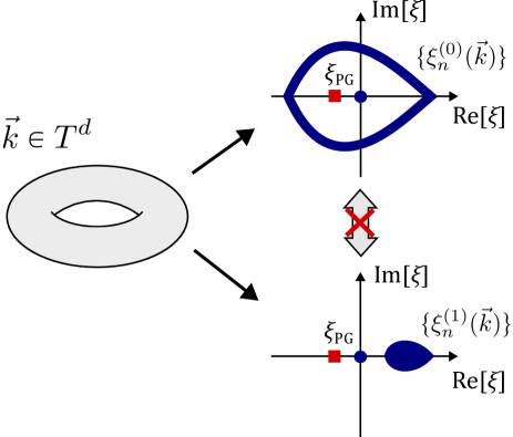
Figure 2: Eigenspectra $\{\xi_{n}^{(0)}(\vec{k})\}$ and $\{\xi_{n}^{(1)}(\vec{k})\}$ (shown by blue areas) of two translationally invariant CPTP maps $\mathcal{E}_{0}$ and $\mathcal{E}_{1}$ that can be calculated from their Bloch matrices defined on the Brillouin zone (the $d$-dimensional torus $T^{d}$). If the Bloch matrices have different values of a topological invariant, the two CPTP maps cannot continuously be deformed to each other without closing the spectral gap. In the figure, a point gap at $\xi_{\mathrm{PG}}$ is depicted by a red square.

Here we note that the Bloch matrix is an $N_{\mathrm{cell}}D_{\mathrm{loc}}^{2}\times N_{\mathrm{cell}}D_{\mathrm{loc}}^{2}$ matrix. Since the size of the matrix diverges in the limit of $N_{\mathrm{cell}}\to\infty$, the definition of a topological invariant of a Bloch matrix is nontrivial. Here we show that this problem can be circumvented by imposing locality on the Kraus operators. We assume that the Kraus operators are local in space and have a finite support. Physically, this implies that the interaction between the system and the measurement apparatus (the feedback controller) is local. Let $\ell$ be the diameter of the support of the Kraus operators, and let $R$ be the range of the Kraus operators. Namely, we assume

$$(\hat{K}_{m})_{\vec{i},a;\vec{j},b}(\hat{K}_{m})^{*}_{\vec{i}^{\prime},c;\vec{j}^{\prime},d}=0\ \mathrm{for}\ |\vec{j}-\vec{j}^{\prime}|>\ell$$ (32)

and

$$(\hat{K}_{m})_{\vec{i},a;\vec{j}.b}=0\ \mathrm{for}\ |\vec{i}-\vec{j}|>R.$$ (33)

We also assume that $\ell$ and $R$ are independent of the system size. Then, we have

$$(\hat{K}_{m})_{\vec{i},a;\vec{j},b}(\hat{K}_{m})^{*}_{\vec{i}^{\prime},c;\vec{j}^{\prime},d}=0\ \mathrm{for}\ |\vec{i}-\vec{i}^{\prime}|>2R+\ell,$$ (34)

since

$$|\vec{i}-\vec{i}^{\prime}|= |\vec{i}-\vec{j}+\vec{j}-\vec{j}^{\prime}+\vec{j}^{\prime}-\vec{i}^{\prime}|$$

$$\leq |\vec{i}-\vec{j}|+|\vec{j}-\vec{j}^{\prime}|+|\vec{i}^{\prime}-\vec{j}^{\prime}|.$$ (35)

The condition (32) leads to

$$X_{a,c,\vec{\mu};b,d,\vec{\nu}}(\vec{k})=0\ \mathrm{for}\ |\vec{\nu}|>\ell.$$ (36)

Furthermore, from the relation (34), we obtain

$$X_{a,c,\vec{\mu};b,d,\vec{\nu}}(\vec{k})=0\ \mathrm{for}\ |\vec{\mu}|>2R+\ell,$$ (37)

which indicates that the Bloch matrix $X(\vec{k})$ can be truncated without changing its nonzero eigenvalues and replaced by a matrix $X_{\mathrm{trunc}}(\vec{k})$ with a finite dimension that does not increase with increasing the system size (see Fig. 3). Hence, topology of CPTP maps can be diagnosed by that of the truncated Bloch matrix $X_{\mathrm{trunc}}(\vec{k})$, which is a finite-size matrix in the $N_{\mathrm{cell}}\to\infty$ limit. Topological feedback control is thus characterized by a topological invariant for the truncated Bloch matrix.

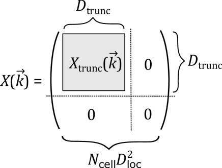
Figure 3: Schematic representation of the Bloch matrix $X(\vec{k})$ which is an $N_{\mathrm{cell}}D_{\mathrm{loc}}^{2}\times N_{\mathrm{cell}}D_{\mathrm{loc}}^{2}$ matrix. If the Kraus operators are local and have a finite support, the Bloch matrix can be truncated into a matrix $X_{\mathrm{trunc}}(\vec{k})$ with dimension $D_{\mathrm{trunc}}$ that remains finite in the limit of $N_{\mathrm{cell}}\to\infty$.

An important consequence of the locality of Kraus operators is that the CPTP map has highly degenerate zero eigenvalues. This can be seen by noting that

$$\hat{K}_{m}\ket{\vec{i},a}\bra{\vec{j},b}\hat{K}_{m}^{\dagger}=0\ \mathrm{for}\ |\vec{i}-\vec{j}|>\ell,$$ (38)

which shows that $\ket{\vec{i},a}\bra{\vec{j},b}$ with $|\vec{i}-\vec{j}|>\ell$ is an eigenoperator of the CPTP map with eigenvalue zero. Thus, the truncation of a Bloch matrix and the highly degenerate zero eigenvalues can be understood as a consequence of local measurement, which erases quantum coherence between distant sites.

The existence of zero eigenvalues of quantum channels implies a crucial difference between dynamics described by those quantum channels and continuous time evolution described by the Lindblad quantum master equation. In fact, a quantum channel $\mathcal{E}$ that has a zero eigenvalue cannot be expressed in terms of any generator $\mathcal{L}$, i.e.,

$$\mathcal{E}\neq e^{\mathcal{L}},$$ (39)

since the right-hand side cannot have a zero eigenvalue. Thus, the topological classification of quantum channels cannot be reduced to that of Lindbladians discussed in literature [64, 65, 66, 67].

III.3 Stable equivalence of quantum channels

In the definition of the equivalence relation in terms of a homotopy presented in the previous subsection, two CPTP maps acting on systems with different numbers of internal degrees of freedom are not homotopic to each other. A more convenient classification of topological phases is obtained by introducing the notion of stable equivalence [18, 27]. In the topological band theory, two band insulators are stably equivalent if they are continuously connected to each other after an addition of some trivial bands [18]. Analogously, we define the stable equivalence of CPTP maps as follows. First, we generalize the quantum states at each unit cell as $\ket{\vec{j},a}$ ($a=1,\cdots,D_{\mathrm{loc}},D_{\mathrm{loc}}+1,\cdots,D_{\mathrm{loc}}+n_{1}$) by adding $n_{1}$ extra local degrees of freedom, which can physically be interpreted as ancillary sublattice sites. We assume that the Kraus operators $\hat{K}_{m}$ act trivially on the extra degrees of freedom, i.e., $\hat{K}_{m}\ket{\vec{j},a}=0$ for $a=D_{\mathrm{loc}}+1,\cdots,D_{\mathrm{loc}}+n_{1}$. Then, we introduce a projective measurement of the ancillary degrees of freedom, which is described by

$$\mathcal{P}_{n_{1}}(\hat{\rho}):=\sum_{\vec{j}}\sum_{a=D_{\mathrm{loc}}+1}^{n_{1}}\hat{P}_{\vec{j},a}\hat{\rho}\hat{P}_{\vec{j},a},$$ (40)

where $\hat{P}_{\vec{j},a}:=\ket{\vec{j},a}\bra{\vec{j},a}$ is the projection operator. The projective measurement channel (40) plays a role of “trivial bands” in the sense that all of its nonzero eigenvalues are unity (see Appendix C). We note that the projection operators $\hat{P}_{\vec{j},a}$ are local in space and therefore in accordance with the discussion in Sec. III.2. We define the direct sum of a quantum channel $\mathcal{E}(\hat{\rho})=\sum_{m}\hat{K}_{m}\hat{\rho}\hat{K}_{m}^{\dagger}$ for the system and the projective measurement channel (40) for the extra bands by

$$(\mathcal{E}\oplus\mathcal{P}_{n_{1}})(\hat{\rho}):=\sum_{m}\hat{K}_{m}\hat{\rho}\hat{K}_{m}^{\dagger}+\sum_{\vec{j}}\sum_{a=D_{\mathrm{loc}}+1}^{n_{1}}\hat{P}_{\vec{j},a}\hat{\rho}\hat{P}_{\vec{j},a}.$$ (41)

Let $\mathcal{E}_{1}$ and $\mathcal{E}_{2}$ be CPTP maps. Then, the CPTP maps $\mathcal{E}_{1}$ and $\mathcal{E}_{2}$ are said to be stably equivalent if and only if $\mathcal{E}_{1}\oplus\mathcal{P}_{n_{1}}$ are homotopic to $\mathcal{E}_{2}\oplus\mathcal{P}_{n_{2}}$ for some two non-negative integers $n_{1}$ and $n_{2}$ (see Fig. 4).

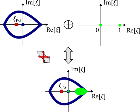
Figure 4: Stable equivalence of CPTP maps. A CPTP map with the eigenspectrum shown by blue areas in the top-left figure is not homotopic to the other CPTP map with the eigenspectrum shown by blue and green areas in the bottom figure, since the numbers of bands (eigenvalues) are different. However, they can be made homotopic if we add a trivial CPTP map with the eigenspectrum shown in the top-right figure.

IV Topological feedback control

IV.1 Chiral Maxwell’s demon

Having established the general framework of topology of quantum channels, here we present a prototypical example of topological quantum feedback control characterized by a topological invariant of the Bloch matrix of a quantum channel. Our model is given by a quantum version of Maxwell’s demon in Ref. [54] (see also Ref. [82]). We consider a particle hopping on a one-dimensional (1D) lattice with $L$ sites, where a quantum state at site $i$ is denoted by $\ket{i}$. We first perform a projective measurement of the position of this particle with measurement operators $\hat{M}_{m}=\ket{m}\bra{m}$ $(m=1,\cdots,L)$. If the measurement outcome is $j$, we raise the potential at site $j-1$ and perform the feedback control with the Hamiltonian

$$\hat{H}_{j}=-J\sum_{i}(\ket{i}\bra{i+1}+\ket{i+1}\bra{i})+V\ket{j-1}\bra{j-1},$$ (42)

where $J\in\mathbb{R}$ is the hopping amplitude and $V>0$ is the height of the potential. The unitary operator for the feedback control is given by $\hat{U}_{j}=\exp[-i\hat{H}_{j}\tau]$, where $\tau$ denotes the duration of the feedback control. The potential barrier placed at site $j-1$ prevents the particle from going to the left, thereby achieving unidirectional (chiral) transport of the particle to the right (see Fig. 5). Here, we do not need any external field to induce the current in the system, but the information obtained from measurement is used to transport the particle. The feedback control thus rectifies quantum fluctuations of measurement outcomes and convert them into a current in a manner similar to an information ratchet [83]. We therefore refer to this model as the chiral Maxwell’s demon.

Figure 5: Schematic illustration of the chiral Maxwell’s demon. A quantum-mechanical particle hops on a one-dimensional lattice with hopping amplitude $J$. We perform a projective measurement of the position of a particle. If we find the particle at site $j$, we raise the potential at site $j-1$ to prevent the particle from hopping to the left.

The eigenvalues $\xi_{n}(k)\ (n=0,\cdots,L-1)$ of a quantum channel of this feedback control can be calculated by using the method described in Appendix B and are given by

$$\xi_{0}(k)=\sum_{r}p(r)e^{-ikr}$$ (43)

and

$$\xi_{1}(k)=\xi_{2}(k)=\cdots=\xi_{L-1}(k)=0,$$ (44)

where

$$p(r)=p(j+r|j):=|(\hat{U}_{j})_{j+r,j}|^{2}$$ (45)

is the probability of finding a particle at site $j+r$ after feedback control with measurement outcome $j$. This probability does not depend on $j$ because of the translational invariance. The zero eigenvalues $\xi_{n\neq 0}(k)$ are due to the projective measurement in which quantum coherence between different sites vanishes: $\hat{M}_{m}\ket{i}\bra{j}\hat{M}_{m}^{\dagger}=0\ (i\neq j)$.

By using the eigenvalues, a topological invariant of the quantum channel is given by the winding number

$$w(\xi_{\mathrm{PG}})=\int_{-\pi}^{\pi}\frac{dk}{2\pi i}\partial_{k}\ln[\xi_{0}(k)-\xi_{\mathrm{PG}}]\in\mathbb{Z},$$ (46)

where $\xi_{\mathrm{PG}}$ denotes the location of a point gap [33]. Here, the eigenvalues $\xi_{n}(k)=0\ (n\neq 0)$ do not contribute to the winding number and thus are excluded from Eq. (46). The winding number takes an integer value and it is invariant under continuous deformation of a feedback control protocol as long as the point gap at $\xi_{\mathrm{PG}}$ is not closed. This is consistent with the $\mathbb{Z}$ classification of non-Hermitian matrices in 1D systems according to stable equivalence [33].

IV.2 Eigenspectrum of a quantum channel under the periodic and open boundary conditions

In Fig. 6, we show the eigenspectrum of a quantum channel for the chiral Maxwell’s demon under the periodic boundary condition (PBC). Beside the highly degenerate zero eigenvalues $\xi_{n\neq 0}(k)$, the loop structure formed by the eigenvalue $\xi_{0}(k)$ can be seen. The winding number is $w(\xi_{\mathrm{PG}})=-1$ for a point gap $\xi_{\mathrm{PG}}$ inside the loop. The eigenvalue $\xi_{0}(k)$ is determined from the probability distribution of the position after feedback control as shown in Eq. (43). In fact, the eigenvalue $\xi_{0}(k)$ is nothing but the characteristic function of the probability distribution $\{p(r)\}$. The chiral transport caused by the feedback control increases the probability of a particle being found at site $r>0$ and makes the probability distribution $\{p(r)\}$ asymmetric with respect to $r>0$ and $r<0$. Thus, the winding number of the quantum channel is intimately related to the chiral transport achieved by the feedback. This physical interpretation is in close analogy with the chiral edge state in the quantum Hall effect and the Hatano-Nelson model for non-Hermitian topological phases [33, 84, 85, 86, 87].

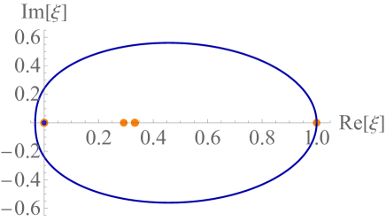
Figure 6: Eigenspectrum of a quantum channel for the chiral Maxwell’s demon. A blue curve and a blue dot constitute the eigenspectrum under the periodic boundary condition in the limit of infinite system size, and orange dots show the eigenspectrum under the open boundary condition with system size $L=50$. The unit of energy is set to $J=1$, and we take $V=+\infty$ for simplicity. The duration of feedback is $\tau=1$.

Nontrivial topology around a point gap under the PBC implies the emergence of a non-Hermitian skin effect under the open boundary condition (OBC) [33, 72, 73, 38, 74]. In Fig. 6, we show the eigenspectrum of the quantum channel under the OBC by orange dots. The eigenspectrum under the OBC is drastically different from that under the PBC, which is a salient feature of the non-Hermitian skin effect. The steady state of the quantum channel under the PBC is uniform in space, while it is localized near the right edge of the system under the OBC [see Fig. 7(a) and (b)]. In Fig. 7(c) and (d), we show a typical behavior of right and left eigenmodes in the OBC. The localization of the right and left eigenmodes at the opposite boundaries of the system indeed confirms the non-Hermitian skin effect, which is a consequence of the chiral transport induced by the chiral Maxwell’s demon.

We note that the localization of right and left eigenmodes $\hat{\rho}_{n}^{L},\hat{\rho}_{n}^{R}$ at opposite edges implies that the overlap $\langle\hat{\rho}_{n}^{L},\hat{\rho}_{n}^{R}\rangle$ decreases exponentially as a function of the system size. From the eigemode expansion (14), this inditates that the expansion coeffecient $c_{n}$ becomes exponentially large, which significantly affects the relaxation dynamics of the system towards the steady state under repeated applications of a quantum channel [88, 89]. Specifically, if the non-Hermitian skin effect takes place, the relaxation time in the OBC generically diverges in the infinite-size limit.

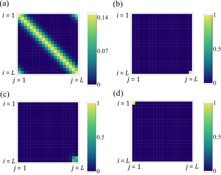
Figure 7: Magnitude $|\rho_{i,j}|$ of matrix elements of an eigenmode $\hat{\rho}_{n}=\sum_{i,j}\rho_{i,j}\ket{i}\bra{j}$ plotted in the position basis for the system size of $L=20$ with the hopping amplitude $J=1$, the height of the potential $V=\infty$, and the duration $\tau=1$ of feedback control. Steady state of the chiral Maxwell’s demon under the PBC (a) and under the OBC (b). Typical right eigenmode (c) and left eigenmode (d) under the OBC. In (c) and (d), eigenmodes with eigenvalue 0.334 are shown.

IV.3 Topological phase transition

The chiral Maxwell’s demon described in Sec. IV.1 exhibits topological phase transitions as the duration $\tau$ of feedback control is changed. In Fig. 8, we show the eigenspectrum under the PBC for four different values of the duration of feedback control. As the duration of feedback control is increased, the absolute value of the winding number also increases. In Fig. 9(a), we show the dependence of the winding number on the duration of feedback control. The topological phase transitions occur at an almost constant rate as a function of the duration.

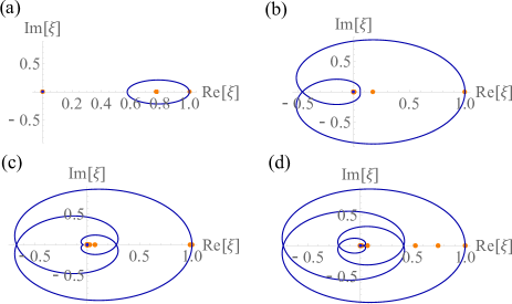
Figure 8: Eigenspectrum of the quantum channel for the chiral Maxwell’s demon for four different values of the duration of the feedback. A blue curve and a blue dot constitute the eigenspectrum under the PBC in the limit of infinite system size, and orange dots show the eigenspectrum under the OBC with the system size of $L=50$. The unit of energy is set to $J=1$, and we take $V=+\infty$. The duration of feedback control is (a) $\tau=0.5$, (b) $\tau=2$, (c) $\tau=3$, and (d) $\tau=3.9$. The winding number $w$ around the origin is (a) $w=0$, (b) $w=-2$, (c) $w=-3$, and (d) $w=-4$.

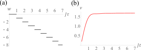
Figure 9: (a) Dependence of the winding number $w(\xi_{\mathrm{PG}}=0)$ on the duration $\tau$ of feedback control. (b) Velocity of a particle during feedback control. The height of the potential is set to be $V=+\infty$.

The topological phase transitions can physically be understood from the ballistic transport of a particle during the feedback control. In Fig. 9(b), we show the mean velocity

$$v(t):=\frac{d}{dt}\sum_{r}r|\bra{j+r}e^{-i\hat{H}_{j}t}\ket{j}|^{2}$$ (47)

of a particle during the feedback control. As seen from the figure, the particle shows ballistic transport at a constant velocity after an initial transient dynamics. To unveil the relation between the ballistic tranport and the topological phase transitions, we rewrite the winding number (46) by using $z=e^{-ik}$ as

$$w(\xi_{\mathrm{PG}}=0)= -\oint_{|z|=1}\frac{dz}{2\pi i}\frac{\xi_{0}^{\prime}(z)}{\xi_{0}(z)},$$ (48)

where

$$\xi_{0}(z):=\sum_{r}p(r)z^{r}$$ (49)

is the probability-generating function of $\{p(r)\}$. From Eq. (48) and by using the argument principle, we have

$$w(\xi_{\mathrm{PG}}=0)=N_{\mathrm{p}}-N_{0},$$ (50)

where $N_{\mathrm{p}}$ ($N_{0}$) is the number of poles (zeros) of the function $\xi_{0}(z)$ in $|z|<1$. The expression (50) gives a physical insight into topological feedback control. Let $\tilde{p}(r):=p(r-1)$ be a shifted probability distribution. Then, its probability-generating function is given by $z\xi_{0}(z)$. It follows then from Eq. (50) that the winding number is changed by $-1$ because the number of zeros is increased by one. The constant increase of the winding number can be understood from the ballistic transport of a particle, since the winding number is changed by $-1$ if the probability distribution of the displacement after feedback control is shifted by one site.

The topological phase transitions are accompanied by exceptional points, at which the CPTP map cannot be diagonalized [68]. In fact, when the value of the winding number around $\xi_{\mathrm{PG}}=0$ changes, $\xi_{0}(k)$ should vanish for some momentum $k$, and the Bloch matrix $X(k)$ cannot be diagonalized at that point (see Appendix B). Thus, here topology causes the emergence of exceptional points of a CPTP map.

V Symmetry classification of feedback control

Symmetry enriches topological phases since two topological phases may be distiguished in the presence of symmetry [18, 17, 19, 27, 28, 33, 34, 35, 65, 37, 66, 67]. Here, we discuss symmetry of quantum channels for discrete quantum feedback control. In Sec. V.1, we discuss unitary symmetry. In Sec. V.2, we consider an antiunitary symmetry associated with every quantum channel. While the contents in these two subsections can be found in literature [90, 91, 33, 92, 66, 67], we reproduce them to make the present paper self-contained. In Sec. V.3, we discuss the Bernard-LeClair (BL) symmetry classes of quantum channels for discrete quantum feedback control. In particular, we find that only a subset of the BL symmetry classes are compatible with projective measurement. Consequently, we obtain the ten-fold symmetry classification of discrete quantum feedback control, as listed in Table 2.

V.1 Unitary symmetry

We first consider unitary symmetry of quantum channels. Similarly to the case of open quantum systems described by the Lindblad equation [90, 91], a unitary symmetry of a quantum channel can be either weak symmetry or strong symmetry [92]. A CPTP map $\mathcal{E}$ has a unitary symmetry if it commutes with a unitary superoperator $\mathcal{V}$, that is,

$$\mathcal{V}\mathcal{E}\mathcal{V}^{-1}=\mathcal{E}.$$ (51)

Let $\tilde{\mathcal{E}}$ be the matrix representation of a CPTP map $\mathcal{E}$ [see Eq. (24)]. Then, Eq. (51) is rewritten as

$$\tilde{\mathcal{V}}\tilde{\mathcal{E}}\tilde{\mathcal{V}}^{-1}=\tilde{\mathcal{E}},$$ (52)

where $\tilde{\mathcal{V}}$ is the matrix representation of $\mathcal{V}$ and given by a unitary operator acting on the doubled Hilbert space $\mathcal{H}\otimes\mathcal{H}$. We call unitary symmetry in Eqs. (51) and (52) as weak symmetry [90, 91, 92]. If a CPTP map has weak symmetry, it can be block-diagonalized according to the symmetry eigenvalues. For example, the translation symmetry in Eq. (25) is a weak symmetry, and the argument $\vec{k}$ of the Bloch matrix $X(\vec{k})$ corresponds to the symmetry eigenvalue (see Appendix A.2).

Suppose that each Kraus operator of a CPTP map commutes with a unitary operator $\hat{V}$ as $[\hat{K}_{m},\hat{V}]=0\ (\forall m)$. Then, the CPTP map satisfies Eq. (52) with $\tilde{\mathcal{V}}=\hat{V}\otimes\hat{I}$ or $\tilde{\mathcal{V}}=\hat{I}\otimes\hat{V}^{*}$. Such symmetry is called strong symmetry [90, 91, 92], which gives a more stringent condition than weak symmetry. Strong symmetry is related to a conserved quantity of the dynamics. To see this, we consider the case of continuous symmetry and assume that each Kraus operator $\hat{K}_{m}$ commutes with $\hat{V}_{\theta}=\exp[-i\theta\hat{A}]$ for all $\theta\in\mathbb{R}$, where $\hat{A}$ is a Hermitian operator. This assumption implies $[\hat{K}_{m},\hat{A}]=0\ (\forall m)$. Then, for an arbitrary density matrix $\hat{\rho}$, we have

$$\mathrm{Tr}[\hat{A}\mathcal{E}(\hat{\rho})]= \sum_{m}\mathrm{Tr}[\hat{K}_{m}^{\dagger}\hat{A}\hat{K}_{m}\hat{\rho}]$$

$$= \mathrm{Tr}\Bigl{[}\Bigl{(}\sum_{m}\hat{K}_{m}^{\dagger}\hat{K}_{m}\Bigr{)}\hat{A}\hat{\rho}\Bigr{]}$$

$$= \mathrm{Tr}[\hat{A}\hat{\rho}],$$ (53)

where we use $\sum_{m}\hat{K}_{m}^{\dagger}\hat{K}_{m}=\hat{I}$ in deriving the last equality. Thus, the observable $\hat{A}$ is conserved under the CPTP map.

V.2 Modular conjugation symmetry

A CPTP map has an antiunitary symmetry due to its Hermiticity-preserving nature [33]. To see this, we define the modular conjugation [93, 66] by an antiunitary operator $\tilde{J}$ acting on the doubled Hilbert space $\mathcal{H}\otimes\mathcal{H}$ as

$$\tilde{J}(\rho_{\vec{i},a;\vec{j},b}\ket{\vec{i},a}\otimes\ket{\vec{j},b}):=\rho_{\vec{i},a;\vec{j},b}^{*}\ket{\vec{j},b}\otimes\ket{\vec{i},a}.$$ (54)

Namely, the modular conjugation operator $\tilde{J}$ is a combination of a swap operation on states and the complex conjugation of their coefficients. The modular conjugation satisfies $\tilde{J}^{2}=1$ and acts on the vectorized density matrix [see Eq. (22)] as

$$\tilde{J}\ket{\hat{\rho}}=\ket{\hat{\rho}^{\dagger}}.$$ (55)

Then, we have

$$\tilde{J}\tilde{\mathcal{E}}\ket{\hat{\rho}}= \tilde{J}\ket{\mathcal{E}(\hat{\rho})}$$

$$= \ket{[\mathcal{E}(\hat{\rho})]^{\dagger}}$$

$$= \ket{\mathcal{E}(\hat{\rho}^{\dagger})}$$

$$= \tilde{\mathcal{E}}\ket{\hat{\rho}^{\dagger}}$$

$$= \tilde{\mathcal{E}}\tilde{J}\ket{\hat{\rho}},$$ (56)

where we use the definition $\tilde{\mathcal{E}}\ket{\hat{\rho}}=\ket{\mathcal{E}(\hat{\rho})}$ of the matrix representation [see Eq. (183)], the property of the modular conjugation [Eq. (55)], and the Hermiticity-preserving condition of a CPTP map [Eq. (16)]. Since Eq. (56) holds for arbitrary $\ket{\hat{\rho}}$, we obtain

$$\tilde{J}\tilde{\mathcal{E}}\tilde{J}^{-1}=\tilde{\mathcal{E}},$$ (57)

which indicates that the operator $\tilde{\mathcal{E}}$ has an antiunitary symmetry defined by the modular conjugation. Since a CPTP map must preserve the Hermiticity of the density matrix, any CPTP map has the modular conjugation symmetry given by Eq. (57).

V.3 Ten-fold symmetry classification of feedback control with projective measurement

The topological classification of non-Hermitian matrices is performed based on the Bernard-LeClair (BL) symmetry classes [75], which are the non-Hermitian generalization [34, 35] of the Altland-Zirnbauer (AZ) symmetry classes [94]. Here, we discuss the BL symmetry classes of quantum channels for discrete quantum feedback control. In general, a symmetry of a CPTP map $\mathcal{E}$ that belongs to a BL symmetry class has one of the following representations [68]:

$$P\ \mathrm{symmetry}:\ \tilde{\mathcal{V}}_{P}\tilde{\mathcal{E}}\tilde{\mathcal{V}}_{P}^{-1}=-\tilde{\mathcal{E}},\ \tilde{\mathcal{V}}_{P}^{2}=\hat{I}\otimes\hat{I},$$ (58a)

$$C\ \mathrm{symmetry}:\ \tilde{\mathcal{V}}_{C}\tilde{\mathcal{E}}^{T}\tilde{\mathcal{V}}_{C}^{-1}=\epsilon_{C}\tilde{\mathcal{E}},\ \tilde{\mathcal{V}}_{C}\tilde{\mathcal{V}}_{C}^{*}=\eta_{C}\hat{I}\otimes\hat{I},$$ (58b)

$$K\ \mathrm{symmetry}:\ \tilde{\mathcal{V}}_{K}\tilde{\mathcal{E}}^{*}\tilde{\mathcal{V}}_{K}^{-1}=\epsilon_{K}\tilde{\mathcal{E}},\ \tilde{\mathcal{V}}_{K}\tilde{\mathcal{V}}_{K}^{*}=\eta_{K}\hat{I}\otimes\hat{I},$$ (58c)

$$Q\ \mathrm{symmetry}:\ \tilde{\mathcal{V}}_{Q}\tilde{\mathcal{E}}^{\dagger}\tilde{\mathcal{V}}_{Q}^{-1}=\epsilon_{Q}\tilde{\mathcal{E}},\ \tilde{\mathcal{V}}_{Q}^{2}=\hat{I}\otimes\hat{I},$$ (58d)

where $\tilde{\mathcal{E}}$ is the matrix representation of $\mathcal{E}$ acting on the doubled Hilbert space (see Sec. III.1), $\tilde{\mathcal{V}}_{X}\ (X=P,C,K,Q)$ is a unitary operator on the doubled Hilbert space, $\epsilon_{X}=\pm 1\ (X=C,K,Q)$, and $\eta_{X}=\pm 1\ (X=C,K)$. Here, we assume that a CPTP map does not have unitary symmetry; if a CPTP map has unitary symmetry, we first block-diagonalize it accoding to the symmetry eigenvalues and consider the BL symmetry class of each block. The combinations of the four types of symmetries (58a)-(58d) lead to 38 classes of non-Hermitian matrices [34].

Whereas general non-Hermitian matrices are classified in terms of the 38 BL symmetry classes [34], some of them are not compatible with CPTP maps for projective measurement. A CPTP map for a projective measurement is given by

$$\mathcal{E}_{\mathrm{proj}}(\hat{\rho})=\sum_{m}\hat{P}_{m}\hat{\rho}\hat{P}_{m},$$ (59)

where $\hat{P}_{m}$ is a projection operator satisfying $\hat{P}_{m}^{\dagger}=\hat{P}_{m}$ and $\hat{P}_{m}\hat{P}_{m^{\prime}}=\delta_{m,m^{\prime}}\hat{P}_{m}$. An important property of the projective measurement channel (59) is that its eigenvalues are either zero or one, which follows from the Hermiticity and idempotence of projection operators (see Appendix C for the proof). Physically, this property is related to the repeatability of projective measurements, that is, repeated projective measurements after a projective measurement with outcome $m$ always yield the same outcome $m$ [47]. To identify the possible symmetry classes of the projective measurement channel (59), we note that a certain BL symmetry places a constraint on the eigenvalues of a CPTP map. Let $\xi$ be an eigenvalue of a CPTP map $\mathcal{E}$. Then, if this CPTP map has $P$ symmetry (58a) or $C$ symmetry with $\epsilon_{C}=-1$, $-\xi$ is also an eigenvalue of $\mathcal{E}$ [68]. Similarly, if a CPTP map $\mathcal{E}$ has $K$ ($Q$) symmetry, $\epsilon_{K}\xi^{*}$ ($\epsilon_{Q}\xi^{*}$) is also an eigenvalue of $\mathcal{E}$. Since a projective measurement channel (59) always has an eigenvalue $+1$ but cannot have an eigenvalue $-1$, we conclude that $P$ symmetry and $X=C,K,Q$ symmetry with $\epsilon_{X}=-1$ cannot be a symmetry of the projective measurement channel (see Fig. 10). Thus, the possible symmetries of a CPTP map for projective measurement are the following ones:

$$\tilde{\mathcal{V}}_{C}\tilde{\mathcal{E}}^{T}\tilde{\mathcal{V}}_{C}^{-1}= \tilde{\mathcal{E}},\ \tilde{\mathcal{V}}_{C}\tilde{\mathcal{V}}_{C}^{*}=\eta_{C}\hat{I}\otimes\hat{I},$$ (60a)

$$\tilde{\mathcal{V}}_{K}\tilde{\mathcal{E}}^{*}\tilde{\mathcal{V}}_{K}^{-1}= \tilde{\mathcal{E}},\ \tilde{\mathcal{V}}_{K}\tilde{\mathcal{V}}_{K}^{*}=\eta_{K}\hat{I}\otimes\hat{I},$$ (60b)

$$\tilde{\mathcal{V}}_{Q}\tilde{\mathcal{E}}^{\dagger}\tilde{\mathcal{V}}_{Q}^{-1}= \tilde{\mathcal{E}},\ \tilde{\mathcal{V}}_{Q}^{2}=\hat{I}\otimes\hat{I},$$ (60c)

where $\eta_{C},\eta_{K}=\pm 1$, and $\tilde{\mathcal{V}}_{K},\tilde{\mathcal{V}}_{K},\tilde{\mathcal{V}}_{Q}$ are unitary operators on the doubled Hilbert space.

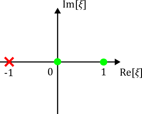
Figure 10: Eigenspectrum of a projective measurement channel (shown by green dots) consisting of eigenvalues zero and one. Since a projective measurement channel cannot have eigenvalue $-1$, its possible BL symmetry classes are restricted to a subset of the entire 38 symmetry classes.

Now let us consider quantum channels for discrete quantum feedback control with projective measurement. Specifically, here we consider a CPTP map of the form

$$\mathcal{E}_{\tau}(\hat{\rho})=\sum_{m}\hat{U}_{m}(\tau)\hat{P}_{m}\hat{\rho}\hat{P}_{m}\hat{U}_{m}^{\dagger}(\tau),$$ (61)

where $\hat{U}_{m}(\tau)=\mathcal{T}\exp\Bigl{[}-i\int_{0}^{\tau}dt\hat{H}_{m}(t)\Bigr{]}$ is the feedback unitary operator generated by a Hamiltonian $\hat{H}_{m}(t)$. Since relevant symmetry of feedback control described by the CPTP map (61) should not depend on the duration $\tau$ of feedback control, it should be consistent with the symmetry in the limit of $\tau\to 0$, where the CPTP map reduces to the projective measurement channel as $\lim_{\tau\to 0}\mathcal{E}_{\tau}=\mathcal{E}_{\mathrm{proj}}$. Thus, the BL symmetries that are allowed for the CPTP map (61) are given by the same symmetries in Eqs. (60a)-(60c).

The three types of symmetries (60a)-(60c) and the combinations thereof constitute ten symmetry classes of quantum channels for discrete quantum feedback control with projective measurement. Notably, they belong to a subset of the entire 38 BL symmetry classes applicable to general non-Hemitian systems [34, 35]. Each symmetry class is specified by the presence or absence of the three types of symmetries (60a)-(60c) and by the signs of $\eta_{C}$ and $\eta_{K}$, as shown in Table 2. Here, it is sufficient to consider a single symmetry for each type (60a)-(60c). In fact, if a system has multiple symmetries of the same type, we can construct a unitary symmetry by combining the two BL symmetries. We note that the existence of two symmetries among (60a)-(60c) leads to the presence of the remaining symmetry constructed from the combination of the two symmetry operations, resulting in ten classes.

We list the ten-fold symmetry classification of quantum channels in Table 2, where each symmetry class is labeled according to the general classification of non-Hermitian symmetry classes in Ref. [34]. We note that these ten symmetry classes are equivalent to the AZ^† classes in Ref. [34] if we multiply $i$ to the original CPTP maps. In fact, the $C$ symmetry (60a) and the $K$ symmetry (60b) are equivalent to “time-reversal symmetry^†” and “particle-hole symmetry^†” of $i\tilde{\mathcal{E}}$, respectively [95, 34]. In Table 2, we also show the AZ^† classes corresponding to the symmetry classes of CPTP maps.

Once the relevant symmetry classes are identified, we can exploit the topological classification of general non-Hermitian matrices [34, 35] to examine whether there exists topological feedback control that is described by a topologically nontrivial Bloch matrix in a given symmetry class and spatial dimension. We note, however, that the Bloch matrix cannot be a general non-Hermitian matrix due to the completely positivity and trace-preserving nature of quantum channels (see Appendix A.4). In particular, the complete positivity may place nontrivial constraints on possible topological phases realized with feedback control. We will present an example of this phenomenon in Sec. VI.2.

The present symmetry classification applies to the case with multipoint projective measurements. For example, if a CPTP map for feedback control with a two-point projective measurement is written as

$$\mathcal{E}_{\tau_{1},\tau_{2}}^{\prime}(\hat{\rho})=\sum_{m_{1},m_{2}}\hat{U}_{m_{1},m_{2}}^{\prime}(\tau_{2})\hat{P}_{m_{2}}\hat{U}_{m_{1}}(\tau_{1})\hat{P}_{m_{1}}\hat{\rho}\hat{P}_{m_{1}}\hat{U}_{m_{1}}^{\dagger}(\tau_{1})\hat{P}_{m_{2}}\hat{U}_{m_{1},m_{2}}^{\prime{\dagger}}(\tau_{2}),$$ (62)

where $\hat{U}_{m_{1},m_{2}}^{\prime}(\tau_{2})=\mathcal{T}\exp[-i\int_{0}^{\tau_{2}}dt\hat{H}_{m_{1},m_{2}}^{\prime}(t)]$ is a unitary operator generated by a Hamiltonian $\hat{H}_{m_{1},m_{2}}^{\prime}(t)$, the “no-feedback” limit again reduces to the projective measurement channel as $\lim_{\tau_{1},\tau_{2}\to 0}\mathcal{E}_{\tau_{1},\tau_{2}}^{\prime}=\mathcal{E}_{\mathrm{proj}}$. Thus, the allowed symmetry classes for CPTP maps (62) for two-point projective measurements are again given by the ten classes in Table 2. Here, we assume that the measurement operators for the second measurement are the same as those of the first measurement given in Eq. (62). If the measurement operators are different for the two measurements, other BL symmetry classes may be allowed. We will discuss this possibility in Sec. IX.

Even if a measurement is not projective, other symmetry classes are still not allowed as long as eigenvalues of a CPTP map for measurement do not always appear as pairs like $(\xi,-\xi)$ or $(\xi,-\xi^{*})$. For example, if a measurement is not projective due to an error in the measurement process, the possible symmetry classes are not altered because we can take an error-free limit under which the symmetry is intact.

The ten AZ^† symmetry classes are formally equivalent to the symmetry classes for generators of Markovian quantum dynamics discussed in Ref. [65]. In fact, the symmetry classes that are given in Table 2 are consistent with the symmetry classes of CPTP maps that are generated by Lindbladians (see Appendix D). However, we note that a CPTP map for feedback control cannot have a generator if it has a zero eigenvalue [see Eq. (39)]. In general, a CPTP map generated by a Lindbladian can be classified by the 38 BL symmetry classes if one includes shifted symmetries [96, 66, 67]. However, a projective measurement channel (59) cannot have those shifted symmetries because the number of zero eigenvalues is different from that of unit eigenvalues, while shifted symmetry is accompanied by the symmetry of the eigenspectrum with respect to a certain line [96, 66, 67]. Thus, we conclude that the ten-fold symmetry classification exhausts all relevant symmetry classes of discrete quantum feedback control with projective measurement.

We note that a CPTP map always has the modular conjugation symmetry [see Eq. (57) in Sec. V.2]. The modular conjugation symmetry corresponds to a $K$ symmetry with $\eta_{K}=+1$. Thus, for symmetry classes that do not include $K$ symmetry with $\eta_{K}=+1$, we require that a CPTP map has a unitary symmetry and consider the BL symmetry class of each symmetry sector, which does not necessarily have the modular conjugation symmetry. We will revisit this point after giving concrete examples in Sec. VI.

Here, we discuss sufficient conditions for the BL symmetries of CPTP maps to satisfy Eqs. (60a)-(60c), which are helpful to gain an insight into feedback control with symmetry. The symmetries in Eqs. (60a), (60b), and (60c) are satisfied if Kraus operators satisfy

$$\tilde{\mathcal{V}}_{C}(\hat{K}_{m}^{T}\otimes\hat{K}_{m}^{\dagger})\tilde{\mathcal{V}}_{C}^{-1}= \hat{K}_{f(m)}\otimes\hat{K}_{f(m)}^{*},$$ (63a)

$$\tilde{\mathcal{V}}_{K}(\hat{K}_{m}^{*}\otimes\hat{K}_{m})\tilde{\mathcal{V}}_{K}^{-1}= \hat{K}_{f(m)}\otimes\hat{K}_{f(m)}^{*},$$ (63b)

$$\tilde{\mathcal{V}}_{Q}(\hat{K}_{m}^{\dagger}\otimes\hat{K}_{m}^{T})\tilde{\mathcal{V}}_{Q}^{-1}= \hat{K}_{f(m)}\otimes\hat{K}_{f(m)}^{*},$$ (63c)

respectively, where $\hat{K}_{m}\ (m=1,2,\cdots,N_{\mathrm{K}})$ are the Kraus operators, $N_{\mathrm{K}}$ is the number of the Kraus operators, and $f$ is a bijection on $\{1,2,\cdots,N_{\mathrm{K}}\}$. Suppose that the Kraus operators of feedback control are given by $\hat{K}_{m}=\hat{U}_{m}\hat{M}_{m}$, where $\hat{M}_{m}$ is a measurement operator and $\hat{U}_{m}=e^{-i\hat{H}_{m}\tau}$ is a unitary operator conditioned on a measurement outcome $m$. Then, if the two conditions

$$\hat{V}_{K}\hat{U}_{m}^{*}\hat{V}_{K}^{-1}=\hat{U}_{m}\ \mathrm{and}\ \hat{V}_{K}\hat{M}_{m}^{*}\hat{V}_{K}^{-1}=e^{i\varphi}\hat{M}_{m}$$ (64)

are satisfied for a unitary operator $\hat{V}_{K}$ and $\varphi\in\mathbb{R}$, Eq. (63b) is satisfied for $f(m)=m$ and $\tilde{\mathcal{V}}_{K}=\hat{V}_{K}\otimes\hat{V}_{K}^{*}$. The first condition in Eq. (64) is equivalent to the particle-hole symmetry of the feedback Hamiltonian (see Eq. (238b) in Appendix D). In this manner, a CPTP map with $K$ symmetry (60b) can be constructed by feedback control with symmetry (64). Since

$$\tilde{\mathcal{V}}_{K}\tilde{\mathcal{V}}_{K}^{*}=\hat{V}_{K}\hat{V}_{K}^{*}\otimes\hat{V}_{K}^{*}\hat{V}_{K},$$ (65)

the condition (64) leads to a $K$ symmetry with $\eta_{K}=+1$ regardless of the sign of $\hat{V}_{K}\hat{V}_{K}^{*}$.

In contrast, the symmetries (60a) and (60c) respectively include transposition and Hermitian conjugation, both of which reverse the order of operators. Because of this order-reversing nature, the symmetries (60a) and (60c) are unlikely to be realized with the simplest protocol involving a single measurement and feedback since $(\hat{U}_{m}\hat{M}_{m})^{T}=\hat{M}_{m}^{T}\hat{U}_{m}^{T}$ and $(\hat{U}_{m}\hat{M}_{m})^{\dagger}=\hat{M}_{m}^{\dagger}\hat{U}_{m}^{\dagger}$. We will demonstrate in Sec. VI that those symmetries can be satisfied by a protocol with a two-point measurement before and after feedback control, where the Kraus operators are given by $\hat{K}_{m}=\hat{M}_{m_{2}}\hat{U}_{m_{1}}\hat{M}_{m_{1}}$ with $m=(m_{1},m_{2})$ being a pair of measurement outcomes (see Sec. II).

VI Feedback control with symmetry

In this section, we present examples of feedback control for each symmetry class shown in Table 2. On the basis of the intrinsic modular conjugation symmetry (see Sec. V.2), the ten symmetry classes of quantum channels listed in Table 2 can be categorized into three groups according the presence or absense of $K$ symmetry and the sign of $\eta_{K}$. The first group (AI, AI$+$psH₊, and AI$+$psH_-) includes $K$ symmetry with $\eta_{K}=+1$. Since the modular conjugation symmetry features $K$ symmetry with $\eta_{K}=+1$, these symmetry classes can be realized with quantum channels without additional symmetries or with additional $C$ or $Q$ symmetry. The second group (A, psH, AI^†, and AII^†) does not have $K$ symmetry. These classes can be realized in a symmetry sector of a quantun channel with unitary symmetry. The third group (AII, AII$+$psH₊, and AII$+$psH_-) includes $K$ symmetry with $\eta_{K}=-1$. Such symmetry classes can be realized by imposing $K$ symmetry with $\eta_{K}=-1$ on the second group.

VI.1 Class AI: feedback without symmetry or with particle-hole symmetry

We begin with class AI, which includes only $K$ symmetry with $\eta_{K}=+1$. Since a CPTP map always has the modular conjugation symmetry (see Sec. V.2), a quantum channel belongs to class AI if it does not have any other symmetry. For example, the chiral Maxwell’s demon presented in Sec. IV belongs to this class.

A CPTP map can have $K$ symmetry with $\eta_{K}=+1$ that is not equivalent to the modular conjugation symmetry. For example, if the measurement operators and the unitary operators for feedback control satisfy Eq. (64), the corresponding CPTP map has $K$ symmetry. Since the first condition in Eq. (64) follows from the particle-hole symmetry of the feedback Hamiltonian, this symmetry is physically interperted as the particle-hole symmetry in feedback control. If a CPTP map has $K$ symmetry (60b) that is not equivalent to the modular conjugation symmetry, we can construct a unitary symmetry

$$\tilde{\mathcal{V}}_{K}\tilde{S}\tilde{\mathcal{E}}(\tilde{\mathcal{V}}_{K}\tilde{S})^{-1}=\tilde{\mathcal{E}},$$ (66)

where $\tilde{S}$ is the swap operator defined by

$$\tilde{S}(\ket{\vec{i},a}\otimes\ket{\vec{j},b})=\ket{\vec{j},b}\otimes\ket{\vec{i},a}.$$ (67)

The CPTP map can be block-diagonalized by using the unitary symmetry (66), and the $K$ symmetry and the modular conjugation symmetry are equivalent in each symmetry sector. Thus, if the CPTP map does not have any other symmetry, the block-diagonalized CPTP map belongs to class AI.

VI.2 Class AI$+$psH₊ and AI$+$psH_-: feedback with a two-point projective measurement

The symmetry classes that include $K$ symmetry with $\eta_{K}=+1$ are class AI, AI$+$psH₊, and AI$+$psH_-, where the last two classes include $C$ and $Q$ symmetries. As mentioned in Sec. V, $C$ and $Q$ symmetries respectively involve transposition and Hermitian conjugation, both of which reverse the order of operators. Here we construct quantum channels with $C$ and $Q$ symmetries by using feedback control with two-point projective measurements. Specifically, we consider a scheme with two projective measurements before and after a unitary operation which is described by a CPTP map

$$\mathcal{E}(\hat{\rho})= \sum_{m_{1},m_{2}}\hat{K}_{m_{1},m_{2}}\hat{\rho}\hat{K}_{m_{1},m_{2}}^{\dagger}$$

$$= \sum_{m_{1},m_{2}}\hat{P}_{m_{2}}\hat{U}_{m_{1}}\hat{P}_{m_{1}}\hat{\rho}\hat{P}_{m_{1}}\hat{U}_{m_{1}}^{\dagger}\hat{P}_{m_{2}},$$ (68)

where $m_{n}=(\vec{j}_{n},a_{n})\ (n=1,2)$ denotes a measurement outcome for a projective measurement with the projection operator $\hat{P}_{m_{n}}:=\hat{P}_{\vec{j}_{n},a_{n}}=\ket{\vec{j}_{n},a_{n}}\bra{\vec{j}_{n},a_{n}}$, and

$$\hat{K}_{m_{1},m_{2}}:= \hat{P}_{m_{2}}\hat{U}_{m_{1}}\hat{P}_{m_{1}}$$

$$= (\hat{U}_{\vec{j}_{1},a_{1}})_{\vec{j}_{2},a_{2};\vec{j}_{1},a_{1}}\ket{\vec{j}_{2},a_{2}}\bra{\vec{j}_{1},a_{1}}$$ (69)

is the Kraus operator. In this case, we have

$$\hat{K}_{m_{1},m_{2}}\otimes\hat{K}_{m_{1},m_{2}}^{*}= p(\vec{j}_{2},a_{2}|\vec{j}_{1},a_{1})$$

$$\times\ket{\vec{j}_{2},a_{2}}\bra{\vec{j}_{1},a_{1}}\otimes\ket{\vec{j}_{2},a_{2}}\bra{\vec{j}_{1},a_{1}}$$ (70)

and

$$\hat{K}_{m_{1},m_{2}}^{T}\otimes\hat{K}_{m_{1},m_{2}}^{\dagger}= p(\vec{j}_{2},a_{2}|\vec{j}_{1},a_{1})$$

$$\times\ket{\vec{j}_{1},a_{1}}\bra{\vec{j}_{2},a_{2}}\otimes\ket{\vec{j}_{1},a_{1}}\bra{\vec{j}_{2},a_{2}},$$ (71)

where $p(\vec{j}_{2},a_{2}|\vec{j}_{1},a_{1}):=|(\hat{U}_{\vec{j}_{1},a_{1}})_{\vec{j}_{2},a_{2};\vec{j}_{1},a_{1}}|^{2}$ is the probability of a measurement outcome $(\vec{j}_{2},a_{2})$ being obtained in the projective measurement performed after feedback control with a measurment outcome $(\vec{j}_{1},a_{1})$. Thus, the conditions (63a) and (63c) for $C$ and $Q$ symmetries follow from symmetry of the transition probability $p(\vec{j}_{2},a_{2}|\vec{j}_{1},a_{1})$.

The Bloch matrix of the CPTP map (68) is given by

$$X_{a,c,\vec{\mu};b,d,\vec{\nu}}(\vec{k})= \frac{1}{N_{\mathrm{cell}}}\sum_{\vec{j},\vec{j}^{\prime}}\sum_{m_{1},m_{2}}(\hat{K}_{m_{1},m_{2}})_{\vec{j},a;\vec{j}^{\prime},b}$$

$$\times(\hat{K}_{m_{1},m_{2}})^{*}_{\vec{j}+\vec{\mu},c;\vec{j}^{\prime}+\vec{\nu},d}e^{-i\vec{k}\cdot(\vec{R}_{\vec{j}}-\vec{R}_{\vec{j}^{\prime}})}$$

$$= \delta_{\vec{\mu},\vec{0}}\delta_{\vec{\nu},\vec{0}}\delta_{a,c}\delta_{b,d}\frac{1}{N_{\mathrm{cell}}}\sum_{\vec{j}_{1},\vec{j}_{2}}p(\vec{j}_{2},a|\vec{j}_{1},b)$$

$$\times e^{-i\vec{k}\cdot(\vec{R}_{\vec{j}_{2}}-\vec{R}_{\vec{j}_{1}})}.$$ (72)

Thus, the Bloch matrix has the following structure

$$X(\vec{k})=\begin{pmatrix}X_{\mathrm{trunc}}(\vec{k})&O\\ O&O\end{pmatrix},$$ (73)

where

$$X_{\mathrm{trunc}}(\vec{k})=\begin{pmatrix}X_{1,1,\vec{0};1,1,\vec{0}}(\vec{k})&X_{1,1,\vec{0};2,2,\vec{0}}(\vec{k})&\cdots&X_{1,1,\vec{0};D_{\mathrm{loc}},D_{\mathrm{loc}},\vec{0}}(k)\\ X_{2,2,\vec{0};1,1,\vec{0}}(\vec{k})&X_{2,2,\vec{0};2,2,\vec{0}}(\vec{k})&\cdots&X_{2,2,\vec{0};D_{\mathrm{loc}},D_{\mathrm{loc}},\vec{0}}(\vec{k})\\ \vdots&\vdots&&\vdots\\ X_{D_{\mathrm{loc}},D_{\mathrm{loc}},\vec{0};1,1,\vec{0}}(\vec{k})&X_{D_{\mathrm{loc}},D_{\mathrm{loc}},\vec{0};2,2,\vec{0}}(\vec{k})&\cdots&X_{D_{\mathrm{loc}},D_{\mathrm{loc}},\vec{0};D_{\mathrm{loc}},D_{\mathrm{loc}},\vec{0}}(\vec{k})\\ \end{pmatrix}$$ (74)

is the truncated Bloch matrix. Nonzero eigenvalues of the Bloch matrix are completely determined by those of the truncated Bloch matrix. The BL symmetry class of the Bloch matrix is also determined from that of the truncated Bloch matrix.

By way of illustration, we consider a system with a spin-$1/2$ particle, which corresponds to the case with $D_{\mathrm{loc}}=2$. The truncated Bloch matrix is given by

$$X_{\mathrm{trunc}}(\vec{k})=\begin{pmatrix}\xi_{\uparrow\uparrow}(\vec{k})&\xi_{\uparrow\downarrow}(\vec{k})\\ \xi_{\downarrow\uparrow}(\vec{k})&\xi_{\downarrow\downarrow}(\vec{k})\end{pmatrix},$$ (75)

where

$$\xi_{\sigma\sigma^{\prime}}(\vec{k}):= X_{\sigma,\sigma,\vec{0};\sigma^{\prime},\sigma^{\prime},\vec{0}}(\vec{k})$$

$$= \frac{1}{N_{\mathrm{cell}}}\sum_{\vec{j}_{1},\vec{j}_{2}}p(\vec{j}_{2},\sigma|\vec{j}_{1},\sigma^{\prime})e^{-i\vec{k}\cdot(\vec{R}_{\vec{j}_{2}}-\vec{R}_{\vec{j}_{1}})}.$$ (76)

Let us examine the symmetry of the truncated Bloch matrix. First, we note that the truncated Bloch matrix always has an antiunitary symmetry (the modular conjugation symmetry)

$$X_{\mathrm{trunc}}^{*}(-\vec{k})=X_{\mathrm{trunc}}(\vec{k})$$ (77)

due to the Hermiticity-preserving nature of the CPTP map (see Sec. V.2 and Appendix A.4). This corresponds to $K$ symmetry (60b) with $\eta_{K}=+1$. Next, we consider $C$ symmetry (60a). The simplest symmetry of this type with $\eta_{C}=+1$ is given by

$$X_{\mathrm{trunc}}^{T}(-\vec{k})=X_{\mathrm{trunc}}(\vec{k}),$$ (78)

which is equivalent to the condition

$$\xi_{\sigma\sigma^{\prime}}(-\vec{k})=\xi_{\sigma^{\prime}\sigma}(\vec{k}).$$ (79)

The condition (79) is satisfied if

$$p(\vec{j}_{2},\sigma|\vec{j}_{1},\sigma^{\prime})=p(\vec{j}_{1},\sigma^{\prime}|\vec{j}_{2},\sigma),$$ (80)

which can be interpreted as reciprocity in the feedback process. The truncated Bloch matrix (and hence the Bloch matrix) with Eq. (78) belongs to the symmetry class AI$+$psH₊ in Table 2. In the present case with Eqs. (77) and (78), the truncated Bloch matrix is Hermitian ($X_{\mathrm{trunc}}^{\dagger}(\vec{k})=X_{\mathrm{trunc}}(\vec{k})$), and therefore its eigenvalues are real. More specifically, the truncated Bloch matrix in a 1D system cannot have a nonzero winding number in the complex plane.

Another symmetry class AI$+$psH_- possesses $C$ symmetry with $\eta_{C}=-1$. An example of such symmetry is given by

$$(-i\sigma_{y})X_{\mathrm{trunc}}^{T}(-\vec{k})(-i\sigma_{y})^{-1}=X_{\mathrm{trunc}}(\vec{k}),$$ (81)

where $\sigma_{y}$ is the Pauli matrix. This type of symmetry leads to the Kramers degeneracy in non-Hermitian systems [34]. The symmetry (81) is equivalent to the following three conditions:

$$\xi_{\uparrow\uparrow}(-\vec{k})= \xi_{\downarrow\downarrow}(\vec{k}),$$ (82a)

$$\xi_{\uparrow\downarrow}(-\vec{k})= -\xi_{\uparrow\downarrow}(\vec{k}),$$ (82b)

$$\xi_{\downarrow\uparrow}(-\vec{k})= -\xi_{\downarrow\uparrow}(\vec{k}).$$ (82c)

The condition (82a) is satisfied if

$$p(\vec{j}_{2},\uparrow|\vec{j}_{1},\uparrow)=p(\vec{j}_{1},\downarrow|\vec{j}_{2},\downarrow),$$ (83)

which represents the reciprocity in which the the two spin components flow in opposite directions. In contrast, since $p(\vec{j}_{2},\sigma|\vec{j}_{1},\sigma^{\prime})\geq 0$, the conditions (82b) and (82c) are satisfied if and only if

$$p(\vec{j}_{2},\uparrow|\vec{j}_{1},\downarrow)=p(\vec{j}_{2},\downarrow|\vec{j}_{1},\uparrow)=0\ (\forall\vec{j}_{1},\vec{j}_{2}).$$ (84)

This means that the truncated Bloch matrix is written as

$$X_{\mathrm{trunc}}(\vec{k})=\begin{pmatrix}\xi_{\uparrow\uparrow}(\vec{k})&0\\ 0&\xi_{\downarrow\downarrow}(\vec{k})\end{pmatrix}.$$ (85)

This matrix actually possesses a higher symmetry; the two spin sectors are completely decoupled and the probability in each sector is separately conserved. This is because the Bloch matrix cannot be an arbitrary non-Hermitian matrix; it must respect the complete positivity and the trace-preserving property of the original CPTP map. This implies that the CPTP properties impose nontrivial constraints on the symmetry of CPTP maps, which may also have an impact on the topological classification.

VI.3 Class A, AI^†, AII^†, and psH: feedback with unitary symmetry

VI.3.1 Class A

Since a CPTP map always has the modular conjugation symmetry, a CPTP map in a class without $K$ symmetry requires unitary symmetry by which the Bloch matrix can be block-diagonalized, as explained in Sec. V. Here, we explicitly construct such examples of feedback control with unitary symmetry.

Let $\{\hat{M}_{m}\}$ be measurement operators. We assume that the measurement operators commute with an observable $\hat{C}$: $[\hat{M}_{m},\hat{C}]=0\ (\forall m)$. Such measurement operators describe a quantum nondemolition (QND) measurement for the observable $\hat{C}$ in the sense that all moments of $\hat{C}$ before and after the measurement stay the same [97], which can be shown as

$$\sum_{m}\mathrm{Tr}[\hat{C}^{r}\hat{M}_{m}\hat{\rho}\hat{M}_{m}^{\dagger}]= \sum_{m}\mathrm{Tr}[\hat{M}_{m}^{\dagger}\hat{M}_{m}\hat{C}^{r}\hat{\rho}]$$

$$= \mathrm{Tr}[\hat{C}^{r}\hat{\rho}]$$ (86)

for arbitrary $\hat{\rho}$ and $r\in\mathbb{N}$. We further assume that the feedback Hamiltonian $\hat{H}_{m}$ commutes with $\hat{C}$, i.e., $[\hat{H}_{m},\hat{C}]=0$ so that $\hat{C}$ is conserved during the feedback control. Then, it follows that the Kraus operator $\hat{K}_{m}=\hat{U}_{m}\hat{M}_{m}$ with $\hat{U}_{m}=\exp[-i\hat{H}_{m}\tau]$ commutes with $\hat{C}$: $[\hat{K}_{m},\hat{C}]=0\ (\forall m)$. Thus, the CPTP map for this feedback control has strong symmetry (see Sec. V.1).

By using strong symmetry, the CPTP map for the feedback control can be block-diagonalized according to the symmetry eigenvalues for the ket and bra spaces. Let

$$\hat{C}=\sum_{c}c\hat{Q}_{c}$$ (87)

be the spectral decomposition of $\hat{C}$, where $c$ is an eigenvalue of $\hat{C}$ and $\hat{Q}_{c}$ is the projection operator onto the corresponding eigenspace $\mathcal{H}_{c}$. Then, the doubled Hilbert space is decomposed as

$$\mathcal{H}\otimes\mathcal{H}=\bigoplus_{c,c^{\prime}}\mathcal{H}_{c}\otimes\mathcal{H}_{c^{\prime}}.$$ (88)

Accordingly, the CPTP map can be decomposed into blocks that act on subspaces with different symmetry eigenvalues. Specifically, we have

$$\tilde{\mathcal{E}}=\sum_{m}\hat{K}_{m}\otimes\hat{K}_{m}^{*}=\sum_{c,c^{\prime}}\tilde{\mathcal{E}}_{c,c^{\prime}},$$ (89)

where

$$\tilde{\mathcal{E}}_{c,c^{\prime}}:=\sum_{m}\hat{K}_{m}\hat{Q}_{c}\otimes\hat{K}_{m}^{*}\hat{Q}_{c^{\prime}}^{*}$$ (90)

acts nontrivialily only on the subspace $\mathcal{H}_{c}\otimes\mathcal{H}_{c^{\prime}}$.

The BL symmetry classes are examined for each block-diagonalized matrix $\tilde{\mathcal{E}}_{c,c^{\prime}}$. Here, an important point is that each block does not necessarily have the modular conjugation symmetry since

$$\tilde{J}\tilde{\mathcal{E}}_{c,c^{\prime}}\tilde{J}^{-1}=\tilde{\mathcal{E}}_{c^{\prime},c}.$$ (91)

In particular, $\tilde{\mathcal{E}}_{c,c^{\prime}}$ with $c\neq c^{\prime}$ does not possess the modular conjugation symmetry, but it is related to $\tilde{\mathcal{E}}_{c^{\prime},c}$ by this symmetry. Since neither of $\tilde{\mathcal{E}}_{c,c^{\prime}}$ nor $\tilde{\mathcal{E}}_{c^{\prime},c}$ with $c\neq c^{\prime}$ is constrained by the modular conjugation symmetry, it belongs to class A if it does not have any other symmetry.

VI.3.2 Class AI^†

The other classes (psH, AI^†, and AII^†) without $K$ symmetry include $C$ or $Q$ symmetry. These symmetries are realized with feedback protocols with two-point measurements simialar to those in Sec. VII.2. Specifically, we consider a spin-$1/2$ particle with two sublattice degrees of freedom, where a quantum state at site $\vec{j}$ with sublattice $a=A,B$ and spin $\sigma=\uparrow,\downarrow$ is denoted by $\ket{\vec{j},a,\sigma}$. We perform a projective position measurement on this particle, and assume that this measurement does not disturb the spin state of the particle. Thus, a measurement outcome is specified only by the site index $\vec{j}$ and the sublattice index $a$, and the measurement operator is given by

$$\hat{M}_{\vec{j},a}=\ket{\vec{j},a,\uparrow}\bra{\vec{j},a,\uparrow}+\ket{\vec{j},a,\downarrow}\bra{\vec{j},a,\downarrow}.$$ (92)

The measurement operator satisfies $[\hat{M}_{\vec{j},a},\hat{S}^{z}]=0$, where

$$\hat{S}^{z}=\frac{1}{2}\sum_{\vec{i},a}(\ket{\vec{i},a,\uparrow}\bra{\vec{i},a,\uparrow}-\ket{\vec{i},a,\downarrow}\bra{\vec{i},a,\downarrow})$$ (93)

is the magnetization. A physical example of such a measurement is given by the position measurement of an atom with nuclear spin degrees of freedom, in which the measurement process does not alter the nuclear-spin states.

We consider a CPTP map

$$\mathcal{E}(\hat{\rho})= \sum_{m_{1},m_{2}}\hat{K}_{m_{1},m_{2}}\hat{\rho}\hat{K}_{m_{1},m_{2}}^{\dagger},$$ (94)

where $\hat{K}_{m_{1},m_{2}}=\hat{M}_{m_{2}}\hat{U}_{m_{1}}\hat{M}_{m_{1}}$ is the Kraus operator, $\hat{M}_{m}$ is the measurment operator (92) corresponding to a measurement outcome $m=(\vec{j},a)$, and $\hat{U}_{m}$ is a unitary operator for a feedback operation. We assume that $[\hat{U}_{m},\hat{S}^{z}]=0$. As in the case of a single measurement in Sec. VI.3.1, the CPTP map can be decomposed as

$$\tilde{\mathcal{E}}= \sum_{m_{1},m_{2}}\hat{K}_{m_{1},m_{2}}\otimes\hat{K}_{m_{1},m_{2}}^{*}$$

$$= \tilde{\mathcal{E}}_{\uparrow\uparrow}+\tilde{\mathcal{E}}_{\uparrow\downarrow}+\tilde{\mathcal{E}}_{\downarrow\uparrow}+\tilde{\mathcal{E}}_{\downarrow\downarrow},$$ (95)

where

$$\tilde{\mathcal{E}}_{\sigma\sigma^{\prime}}=\sum_{\vec{j}_{1},a_{1},\vec{j}_{2},a_{2}} \hat{M}_{\vec{j}_{2},a_{2},\sigma}\hat{U}_{\vec{j}_{1},a_{1}}\hat{M}_{\vec{j}_{1},a_{1},\sigma}$$

$$\otimes\hat{M}_{\vec{j}_{2},a_{2},\sigma^{\prime}}^{*}\hat{U}_{\vec{j}_{1},a_{1}}^{*}\hat{M}_{\vec{j}_{1},a_{1},\sigma^{\prime}}^{*},$$ (96)

and

$$\hat{M}_{\vec{j},a,\sigma}:=\ket{\vec{j},a,\sigma}\bra{\vec{j},a,\sigma}.$$ (97)

Similarly to the analysis in Sec. VI.2, the Bloch matrix for $\tilde{\mathcal{E}}_{\sigma\sigma^{\prime}}$ has a block-diagonal structure (73), and the truncated Bloch matrix is given by

$$X_{\mathrm{trunc}}^{(\sigma\sigma^{\prime})}(\vec{k})=\begin{pmatrix}\xi_{AA}^{(\sigma\sigma^{\prime})}(\vec{k})&\xi_{AB}^{(\sigma\sigma^{\prime})}(\vec{k})\\ \xi_{BA}^{(\sigma\sigma^{\prime})}(\vec{k})&\xi_{BB}^{(\sigma\sigma^{\prime})}(\vec{k})\end{pmatrix},$$ (98)

where

$$\xi_{ab}^{(\sigma\sigma^{\prime})}(\vec{k})=\frac{1}{N_{\mathrm{cell}}}\sum_{\vec{j}_{1},\vec{j}_{2}}q^{(\sigma\sigma^{\prime})}(\vec{j}_{2},a|\vec{j}_{1},b)e^{-i\vec{k}\cdot(\vec{R}_{\vec{j}_{1}}-\vec{R}_{\vec{j}_{2}})}$$ (99)

with

$$q^{(\sigma\sigma^{\prime})}(\vec{j}_{2},a|\vec{j}_{1},b)=(\hat{U}_{\vec{j}_{1},b})_{\vec{j}_{2},a,\sigma;\vec{j}_{1},b,\sigma}(\hat{U}_{\vec{j}_{1},b})_{\vec{j}_{2},a,\sigma^{\prime};\vec{j}_{1},b,\sigma^{\prime}}^{*}.$$ (100)

For simplicity, here we focus on the truncated Bloch matrix (98) with $\sigma=\uparrow$ and $\sigma^{\prime}=\downarrow$. It has $C$ symmetry with $\eta_{C}=+1$, i.e.,

$$[X_{\mathrm{trunc}}^{(\uparrow\downarrow)}(-\vec{k})]^{T}=X_{\mathrm{trunc}}^{(\uparrow\downarrow)}(\vec{k})$$ (101)

if

$$\xi_{ab}^{(\uparrow\downarrow)}(-\vec{k})=\xi_{ba}^{(\uparrow\downarrow)}(\vec{k}).$$ (102)

A condition for Eq. (102) is given by

$$q^{(\uparrow\downarrow)}(\vec{j}_{2},a|\vec{j}_{1},b)=q^{(\uparrow\downarrow)}(\vec{j}_{1},b|\vec{j}_{2},a).$$ (103)

This condition is interpreted as reciprocity in the feedback process. Since the truncated Bloch matrix $X_{\mathrm{trunc}}^{(\uparrow\downarrow)}(\vec{k})$ does not have the modular conjugation symmetry, it belongs to the symmetry class AI^†.

VI.3.3 Class AII^†

The symmetry class AII^† involves $C$ symmetry with $\eta_{C}=-1$. Provided that

$$\xi_{AA}^{(\uparrow\downarrow)}(-\vec{k})= \xi_{BB}^{(\uparrow\downarrow)}(\vec{k}),$$ (104a)

$$\xi_{AB}^{(\uparrow\downarrow)}(-\vec{k})= -\xi_{AB}^{(\uparrow\downarrow)}(\vec{k}),$$ (104b)

$$\xi_{BA}^{(\uparrow\downarrow)}(-\vec{k})= -\xi_{BA}^{(\uparrow\downarrow)}(\vec{k}),$$ (104c)

the truncated Bloch matrix $X_{\mathrm{trunc}}^{(\uparrow\downarrow)}(\vec{k})$ has $C$ symmetry with $\eta_{C}=-1$:

$$(-i\sigma_{y})[X_{\mathrm{trunc}}^{(\uparrow\downarrow)}(-\vec{k})]^{T}(-i\sigma_{y})^{-1}=X_{\mathrm{trunc}}^{(\uparrow\downarrow)}(\vec{k}).$$ (105)

The conditions for this symmetry are given by

$$q^{(\uparrow\downarrow)}(\vec{j}_{2},A|\vec{j}_{1},A)= q^{(\uparrow\downarrow)}(\vec{j}_{1},B|\vec{j}_{2},B),$$ (106a)

$$q^{(\uparrow\downarrow)}(\vec{j}_{2},A|\vec{j}_{1},B)= -q^{(\uparrow\downarrow)}(\vec{j}_{1},A|\vec{j}_{2},B),$$ (106b)

$$q^{(\uparrow\downarrow)}(\vec{j}_{2},B|\vec{j}_{1},A)= -q^{(\uparrow\downarrow)}(\vec{j}_{1},B|\vec{j}_{2},A).$$ (106c)

Here, in sharp contrast to Eqs. (82b) and (82c) in Sec. VI.2, the conditions (104b) and (104c) do not lead to $q^{(\uparrow\downarrow)}(\vec{j}_{2},A|\vec{j}_{1},B)=q^{(\uparrow\downarrow)}(\vec{j}_{2},B|\vec{j}_{1},A)=0$ since $q^{(\uparrow\downarrow)}(\vec{j}_{2},a|\vec{j}_{1},b)$ is not positive semidefinite.

VI.3.4 Class psH

Finally, we consider the condition for $Q$ symmetry, which is also referred to as pseudo-Hermiticity (psH) [34]. An example of psH of the truncated Bloch matrix is given by

$$\sigma_{x}[X_{\mathrm{trunc}}^{(\uparrow\downarrow)}(\vec{k})]^{\dagger}\sigma_{x}^{-1}=X_{\mathrm{trunc}}^{(\uparrow\downarrow)}(\vec{k}),$$ (107)

which is equivalent to

$$[\xi_{AA}^{(\uparrow\downarrow)}(\vec{k})]^{*}= \xi_{BB}^{(\uparrow\downarrow)}(\vec{k}),$$ (108a)

$$[\xi_{AB}^{(\uparrow\downarrow)}(\vec{k})]^{*}= \xi_{AB}^{(\uparrow\downarrow)}(\vec{k}),$$ (108b)

$$[\xi_{BA}^{(\uparrow\downarrow)}(\vec{k})]^{*}= \xi_{BA}^{(\uparrow\downarrow)}(\vec{k}).$$ (108c)

These conditions (108a)-(108c) are satisfied if

$$[q^{(\uparrow\downarrow)}(\vec{j}_{2},A|\vec{j}_{1},A)]^{*}= q^{(\uparrow\downarrow)}(\vec{j}_{1},B|\vec{j}_{2},B),$$ (109a)

$$[q^{(\uparrow\downarrow)}(\vec{j}_{2},A|\vec{j}_{1},B)]^{*}= q^{(\uparrow\downarrow)}(\vec{j}_{1},A|\vec{j}_{2},B),$$ (109b)

$$[q^{(\uparrow\downarrow)}(\vec{j}_{2},B|\vec{j}_{1},A)]^{*}= q^{(\uparrow\downarrow)}(\vec{j}_{1},B|\vec{j}_{2},A).$$ (109c)

In terms of the feedback unitary operators, sufficient conditions for Eqs. (109a)-(109c) are given by

$$(\hat{U}_{\vec{j}_{1},A})_{\vec{j}_{2},A,\sigma;\vec{j}_{1},A,\sigma}^{*}= (\hat{U}_{\vec{j}_{2},B})_{\vec{j}_{1},B,\sigma;\vec{j}_{2},B,\sigma},$$ (110a)

$$(\hat{U}_{\vec{j}_{1},B})_{\vec{j}_{2},A,\sigma;\vec{j}_{1},B,\sigma}^{*}= (\hat{U}_{\vec{j}_{2},B})_{\vec{j}_{1},A,\sigma;\vec{j}_{2},B,\sigma},$$ (110b)

$$(\hat{U}_{\vec{j}_{1},A})_{\vec{j}_{2},B,\sigma;\vec{j}_{1},A,\sigma}^{*}= (\hat{U}_{\vec{j}_{2},A})_{\vec{j}_{1},B,\sigma;\vec{j}_{2},A,\sigma}.$$ (110c)

The psH (107) is understood as a consequence of the modified reciprocity expressed by Eqs. (110a)-(110c).

VI.4 Class AII, AII$+$psH₊, and AII$+$psH_-: feedback with $K$ symmetry and $\eta_{K}=-1$

The remaining symmetry classes include $K$ symmetry with $\eta_{K}=-1$. To implement this symmetry, we consider a system with spin ($\sigma=\uparrow,\downarrow$), orbit ($\ell=s,p$), and sublattice ($a=A,B$) degrees of freedom. We perform a two-point measurement described by measurement operators

$$\hat{M}_{\vec{j},a,\ell}=\ket{\vec{j},a,\ell,\uparrow}\bra{\vec{j},a,\ell,\uparrow}+\ket{\vec{j},a,\ell,\downarrow}\bra{\vec{j},a,\ell,\downarrow}.$$ (111)

We note that these measurement operators make the spin degrees of freedom unaltered. We assume that feedback Hamiltonians conserve the magnetization. Then, a CPTP map for feedback control with a two-point measurement is given by the form (94), where the measurement outcomes are labeled by $m_{n}=(\vec{j}_{n},a_{n},\ell_{n})\ (n=1,2)$. The truncated Bloch matrix is obtained in a manner similar to that in Sec. VI.3.

We impose $K$ symmetry with $\eta_{K}=-1$ on the truncated Bloch matrix as

$$(-i\tau_{y})[X_{\mathrm{trunc}}^{(\uparrow\downarrow)}(-\vec{k})]^{*}(-i\tau_{y})^{-1}=X_{\mathrm{trunc}}^{(\uparrow\downarrow)}(\vec{k}),$$ (112)

where $\tau_{y}$ is the Pauli matrix for the orbital degrees of freedom. This symmetry is equivalent to the conditions

$$[\xi_{a,p;b,p}^{(\uparrow\downarrow)}(-\vec{k})]^{*}= \xi_{a,s;b,s}^{(\uparrow\downarrow)}(\vec{k}),$$ (113a)

$$[\xi_{a,s;b,p}^{(\uparrow\downarrow)}(-\vec{k})]^{*}= -\xi_{a,p;b,s}^{(\uparrow\downarrow)}(\vec{k}),$$ (113b)

where

$$\xi_{a,\ell;b,\ell^{\prime}}^{(\sigma\sigma^{\prime})}(\vec{k})=\frac{1}{N_{\mathrm{cell}}}\sum_{\vec{j}_{1},\vec{j}_{2}}q^{(\sigma\sigma^{\prime})}(\vec{j}_{2},a,\ell|\vec{j}_{1},b,\ell^{\prime})e^{-i\vec{k}\cdot(\vec{R}_{\vec{j}_{1}}-\vec{R}_{\vec{j}_{2}})}$$ (114)

with

$$q^{(\sigma\sigma^{\prime})}(\vec{j}_{2},a,\ell|\vec{j}_{1},b,\ell^{\prime})= (\hat{U}_{\vec{j}_{1},b,\ell^{\prime}})_{\vec{j}_{2},a,\ell,\sigma;\vec{j}_{1},b,\ell^{\prime},\sigma}$$

$$\times(\hat{U}_{\vec{j}_{1},b,\ell^{\prime}})_{\vec{j}_{2},a,\ell,\sigma^{\prime};\vec{j}_{1},b,\ell^{\prime},\sigma^{\prime}}^{*}.$$ (115)

The conditions (113a) and (113b) are satisfied if

$$[q^{(\uparrow\downarrow)}(\vec{j}_{1},a,p|\vec{j}_{2},b,p)]^{*}= q^{(\uparrow\downarrow)}(\vec{j}_{1},a,s|\vec{j}_{2},b,s),$$ (116a)

$$[q^{(\uparrow\downarrow)}(\vec{j}_{1},a,s|\vec{j}_{2},b,p)]^{*}= -q^{(\uparrow\downarrow)}(\vec{j}_{1},a,p|\vec{j}_{2},b,s),$$ (116b)

which represent a type of symmetry in the orbital space.

If we only impose the symmetry (112), the truncated Bloch matrix belongs to class AII. If we further impose $C$ symmetry by using the sublattice degrees of freedom as in Sec. VI.3, we can also realize the truncated Bloch matrix in class AII$+$psH₊ and class AII$+$psH_-.

VII Topological Maxwell’s demons

In this section, builiding on the symmetry classification of quantum channels developed in Sec. V, we present various models of topological feedback control. Speficially, we focus on quantum feedback control of a particle in a 1D lattice and construct topological quantum channels protected by their point-gap topology and symmetry. According to the general topological classification of non-Hermitian operators in Ref. [34], a non-Hermitian operator in a 1D system can host nontrivial point-gap topology in class A, AI, AI$+$psH_-, AII^†, and AII. In Sec. VII.1, we consider topological feedback control in class AI, where we can combine particle-hole symmetry with the modular conjugation symmmetry to construct a unitary symmetry. In Sec. VII.2, we construct a model of topological feedback control in class AI$+$psH_- and demonstrate that it shows helical spin transport protected by $C$ symmetry. Section VII.3 is devoted to topological feedback control in class A, where strong unitary symmetry enables us to block-diagonalize a CPTP map. In Sec. VII.4, we impose strong unitary symmetry and $C$ symmetry on a CPTP map to construct topological feedback control in class AII^†, which exhibits the $\mathbb{Z}_{2}$ skin effect.

VII.1 Su-Schrieffer-Heeger demon

First, we present a model of topological feedback control with $K$ symmetry with $\eta_{K}=+1$ that is distinct from the modular conjugation symmetry. This model provides a concrete example for the discussion presented in Sec. VI.1. We consider a 1D lattice with two sublattices. Each unit cell is labeled by an index $j$ and each sublattice is labeled by $a=A,B$. We first perform projective position measurement which completely resolves the sublattice structure. A measurement outcome is specified by $m=(j,a)$, and the corresponding measurement operator is given by $\hat{M}_{m}=\ket{j,a}\bra{j,a}$. Then, we perform feedback control using Hamiltonian $\hat{H}_{a}\ (a=A,B)$ that depends only on the measurement outcome of the sublattice index. The feedback Hamiltonians are given by the Su-Schrieffer-Heeger (SSH) model [98]

$$\hat{H}_{A}= -J_{1}\sum_{j}(\ket{j,A}\bra{j,B}+\mathrm{H.c.})$$

$$-J_{2}\sum_{i}(\ket{j+1,A}\bra{j,B}+\mathrm{H.c.}),$$ (117)

$$\hat{H}_{B}= -J_{1}^{\prime}\sum_{i}(\ket{j,A}\bra{j,B}+\mathrm{H.c.})$$

$$-J_{2}^{\prime}\sum_{j}(\ket{j+1,A}\bra{j,B}+\mathrm{H.c.}),$$ (118)

where $J_{1},J_{2},J_{1}^{\prime},J_{2}^{\prime}\in\mathbb{R}$ are the hopping amplitudes. See Fig. 11 for a schematic illustration of the feedback protocol. We note that the SSH model has time-reversal symmetry

$$\hat{H}_{a}^{*}=\hat{H}_{a},$$ (119a)

particle-hole symmetry

$$\hat{\Sigma}_{z}\hat{H}_{a}^{*}\hat{\Sigma}_{z}=-\hat{H}_{a},$$ (119b)

and chiral symmetry

$$\hat{\Sigma}_{z}\hat{H}_{a}\hat{\Sigma}_{z}=-\hat{H}_{a},$$ (119c)

where

$$\hat{\Sigma}_{z}=\sum_{j}(\ket{j,A}\bra{j,A}-\ket{j,B}\bra{j,B}).$$ (120)

Note that $\hat{\Sigma}_{z}^{2}=\hat{I}$. Consequently, the unitary time-evolution operator $\hat{U}_{a}=\exp[-i\hat{H}_{a}\tau]$ has the following symmetries (see Appendix D):

$$\hat{U}_{a}^{T}=\hat{U}_{a},$$ (121a)

$$\hat{\Sigma}_{z}\hat{U}_{a}^{*}\hat{\Sigma}_{z}=\hat{U}_{a},$$ (121b)

and

$$\hat{\Sigma}_{z}\hat{U}_{a}^{\dagger}\hat{\Sigma}_{z}=\hat{U}_{a},$$ (121c)

which follow from Eqs. (119a), (119b), and (119c), respectively. Among the symmetries (121a)-(121c), only particle-hole symmetry (121b) leads to the symmetry of a quantum channel for this feedback control. Since the measurement operator satisfies

$$\hat{\Sigma}_{z}\hat{M}_{m}\hat{\Sigma}_{z}=\hat{M}_{m},$$ (122)

particle-hole symmetry (121b) leads to $K$ symmetry

$$(\hat{\Sigma}_{z}\otimes\hat{\Sigma}_{z}^{*})\sum_{m}(\hat{K}_{m}^{*}\otimes\hat{K}_{m})(\hat{\Sigma}_{z}\otimes\hat{\Sigma}_{z}^{*})=\sum_{m}(\hat{K}_{m}\otimes\hat{K}_{m}^{*})$$ (123)

of the CPTP map, where $\hat{K}_{m}=\hat{K}_{(j,a)}=\hat{U}_{a}\hat{M}_{m}$ is the Kraus operator.

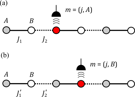
Figure 11: Schematic illustration of the Su-Schrieffer-Heeger (SSH) demon. We first perform projective measurement of the position and the sublattice. (a) If a particle is detected in sublattice $A$, we perform feedback control governed by the Hamiltonian $H_{A}$. (b) If a particle is detected in sublattice $B$, we perform feedback control governed by the Hamiltonian $H_{B}$.

As mentioned in Sec. V, the CPTP map has the modular conjugation symmetry (57), which gives another $K$ symmetry different from (123). Combining the two $K$ symmetries, we obtain the unitary symmetry of the CPTP map as

$$(\Sigma_{z}\otimes\Sigma_{z}^{*})\tilde{S}\sum_{m}(\hat{K}_{m}\otimes\hat{K}_{m}^{*})\tilde{S}^{-1}(\Sigma_{z}\otimes\Sigma_{z}^{*})=\sum_{m}(\hat{K}_{m}\otimes\hat{K}_{m}^{*}),$$ (124)

where $\tilde{S}$ is the swap operator defined by Eq. (67). Hence, the CPTP map can be block-diagonalized according to the symmetry eigenvalues of the unitary symmetry (124). The eigenvalues of $(\hat{\Sigma}_{z}\otimes\hat{\Sigma}_{z})\tilde{S}$ are given by $\pm 1$. The eigenvectors for the eigenvalue $+1$ are given by

$$\ket{j,A}\otimes\ket{j,A},$$ (125a)

$$\ket{j,B}\otimes\ket{j,B},$$ (125b)

$$\frac{1}{\sqrt{2}}(\ket{j,A}\otimes\ket{j^{\prime},B}+\ket{j^{\prime},B}\otimes\ket{j,A}),$$ (125c)

and those for the eigenvalue $-1$ are given by

$$\frac{1}{\sqrt{2}}(\ket{j,A}\otimes\ket{j^{\prime},B}-\ket{j^{\prime},B}\otimes\ket{j,A}).$$ (126)

In each eigenspace of the operator $(\hat{\Sigma}_{z}\otimes\hat{\Sigma}_{z})\tilde{S}$, modular conjugation symmetry (57) and particle-hole symmetry (123) are equivalent to each other since $(\hat{\Sigma}_{z}\otimes\hat{\Sigma}_{z})=\pm\tilde{S}$. Thus, the topological characterization of a CPTP map in those eigenspaces reduces to that of a CPTP map with a single $K$ symmetry. Thus, each symmetry sector of the CPTP map belongs to class AI.

Figure 12 shows the eigenspectrum of a CPTP map for the feedback control with the SSH model under the PBC and that under the OBC. The eigenspectrum under the PBC forms two loops in the complex plane, each of which has the winding number $-1$ for a point gap inside the loop. This nontrivial point-gap topology makes the eigenspectrum under the OBC drastically different from that in the PBC, leading to the non-Hermitian skin effect induced by the SSH demon.

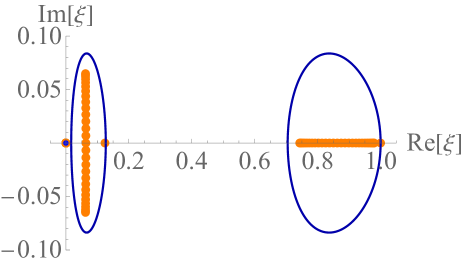
Figure 12: Eigenspectrum of a quantum channel for the SSH demon. Blue curves and the blue dot at the origin constitute the eigenspectrum under the PBC in the infinite-size limit, and orange dots constitute the eigenspectrum under the OBC with the number of unit cells $L=30$. The hopping amplitudes are set to $J_{1}=1,J_{2}=0.5,J_{1}^{\prime}=0.4,J_{2}^{\prime}=0.4$. The duration of feedback is $\tau=1$.

VII.2 Helical Maxwell’s demon

Next, we construct a model of symmetry-protected topological feedback control that belongs to class AI$+$psH_-. We consider a spin-$1/2$ particle on a 1D lattice with $L$ sites. The Hilbert space of this system is spanned by a basis $\{\ket{j,\sigma}\}$ ($j=1,\cdots,L$, $\sigma=\uparrow,\downarrow$). We consider feedback control of this particle with a two-point measurement scheme (see Fig. 13 for a schematic illustration). We first perform a projective measurement of the position and spin with the projection operators $\hat{P}_{j,\sigma}=\ket{j,\sigma}\bra{j,\sigma}$. Let $m_{1}=(j_{1},\sigma_{1})$ be an outcome of this measurement. If we obtain a measurement outcome $(j_{1},\uparrow)$, we raise a spin-independent potential at site $j_{1}-1$ to prevent the particle from going to the left. If we obtain a measurement outcome $(j_{1},\downarrow)$, we raise a spin-independent potential at site $j_{1}+1$ to prevent the particle from going to the right. The feedback Hamiltonians are given by

$$\hat{H}_{j_{1},\uparrow}= -J\sum_{j}\sum_{\sigma}(\ket{j,\sigma}\bra{j+1,\sigma}+\ket{j+1,\sigma}\bra{j,\sigma})$$

$$+V\sum_{\sigma}\ket{j_{1}-1,\sigma}\bra{j_{1}-1,\sigma}$$

$$+h_{x}\sum_{j}(\ket{j,\uparrow}\bra{j,\downarrow}+\ket{j,\downarrow}\bra{j,\uparrow})$$ (127)

and

$$\hat{H}_{j_{1},\downarrow}= -J\sum_{j}\sum_{\sigma}(\ket{j,\sigma}\bra{j+1,\sigma}+\ket{j+1,\sigma}\bra{j,\sigma})$$

$$+V\sum_{\sigma}\ket{j_{1}+1,\sigma}\bra{j_{1}+1,\sigma}$$

$$+h_{x}\sum_{j}(\ket{j,\uparrow}\bra{j,\downarrow}+\ket{j,\downarrow}\bra{j,\uparrow}),$$ (128)

where $J\in\mathbb{R}$ is the hopping amplitude, $V>0$ is the height of the potential, and $h_{x}$ denotes the strength of a transverse magnetic field which mixes the spin components. The feedback control is described by a unitary operator $\hat{U}_{j_{1},\sigma_{1}}=\exp[-i\hat{H}_{j_{1},\sigma_{1}}\tau]$. After the feedback control, we perform the second projective measurement with projection operators $\hat{P}_{j,\sigma}$. Let $m_{2}=(j_{2},\sigma_{2})$ be an outcome of this second measurement. If $\sigma_{2}=\sigma_{1}$, we do nothing. If $\sigma_{2}\neq\sigma_{1}$, we flip the spin of the particle by applying a $\pi$ pulse of a magnetic field. Through this feedback control, a spin-up particle is transported to the right, while a spin-down particle is transported to the left, which is analogous to helical edge states in the quantum spin Hall effect [12, 13, 14, 15, 16]

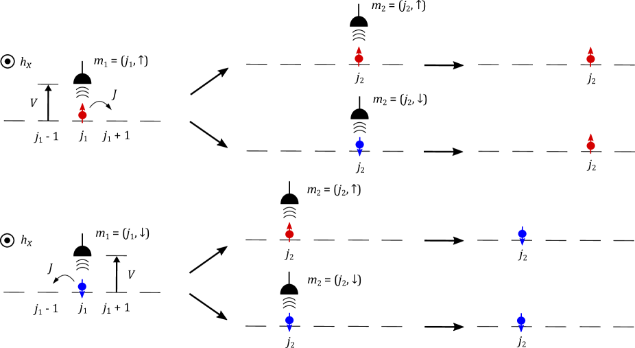
Figure 13: Schematic illustration of the helical Maxwell’s demon for a spin-$1/2$ particle on a 1D lattice. We first perform a projective measurement of the position and spin of the particle. If we obtain an outcome $m_{1}=(j_{1},\uparrow)$ ($m_{1}=(j_{1},\downarrow)$), we raise the potential at site $j_{1}-1$ ($j+1$) and let the particle undergo unitary time evolution under the feedback Hamiltonian given in Eq. (127) (Eq. (128)). After that, we perform the second projective measurement of the position and spin. If the measurement outcome of spin is different from that of the first measurement, we apply a $\pi$ pulse of a magnetic field to flip the spin with unit probability. Thus, helical spin transport is achieved.

The quantum channel for the entire process of this feedback control is given by

$$\mathcal{E}(\hat{\rho})=\sum_{m_{1},m_{2}}\hat{K}_{m_{1},m_{2}}\hat{\rho}\hat{K}_{m_{1},m_{2}}^{\dagger},$$ (129)

where the Kraus operators are given by

$$\hat{K}_{(j_{1},\uparrow),(j_{2},\uparrow)}= \ket{j_{2},\uparrow}\bra{j_{2},\uparrow}\hat{U}_{j_{1},\uparrow}\ket{j_{1},\uparrow}\bra{j_{1},\uparrow},$$ (130a)

$$\hat{K}_{(j_{1},\downarrow),(j_{2},\downarrow)}= \ket{j_{2},\downarrow}\bra{j_{2},\downarrow}\hat{U}_{j_{1},\downarrow}\ket{j_{1},\downarrow}\bra{j_{1},\downarrow},$$ (130b)

$$\hat{K}_{(j_{1},\uparrow),(j_{2},\downarrow)}= \ket{j_{2},\uparrow}\bra{j_{2},\downarrow}\hat{U}_{j_{1},\uparrow}\ket{j_{1},\uparrow}\bra{j_{1},\uparrow},$$ (130c)

$$\hat{K}_{(j_{1},\downarrow),(j_{2},\uparrow)}= \ket{j_{2},\downarrow}\bra{j_{2},\uparrow}\hat{U}_{j_{1},\downarrow}\ket{j_{1},\downarrow}\bra{j_{1},\downarrow}.$$ (130d)

The Bloch matrix of this quantum channel has the structure in Eq. (73) and is given by

$$X(k)=\begin{pmatrix}X_{\mathrm{trunc}}(k)&O\\ O&O\end{pmatrix},$$ (131)

where

$$X_{\mathrm{trunc}}(k)=\begin{pmatrix}\xi_{\uparrow\uparrow}(k)+\xi_{\downarrow\uparrow}(k)&0\\ 0&\xi_{\downarrow\downarrow}(k)+\xi_{\uparrow\downarrow}(k)\end{pmatrix}$$ (132)

and

$$\xi_{\sigma\sigma^{\prime}}(k)= \frac{1}{L}\sum_{j_{1},j_{2}}|\bra{j_{2},\sigma}\hat{U}_{j_{1},\sigma^{\prime}}\ket{j_{1},\sigma^{\prime}}|^{2}e^{-ik(j_{2}-j_{1})}.$$ (133)

Note that we can transfer the off-diagonal components in Eq. (75) to the diagonal components by the additional feedback control after the second measurement. The truncated Bloch matrix has the symmetry

$$(-i\sigma_{y})X_{\mathrm{trunc}}^{T}(-k)(-i\sigma_{y})^{-1}=X_{\mathrm{trunc}}(k),$$ (134)

which corresponds to $C$ symmetry (60a) of the CPTP map with $\eta_{C}=-1$, since

$$\xi_{\uparrow\uparrow}(-k)=\xi_{\downarrow\downarrow}(k)$$ (135a)

and

$$\xi_{\uparrow\downarrow}(-k)=\xi_{\downarrow\uparrow}(k)$$ (135b)

hold due to the symmetry of the feedback protocol. Thus, the Bloch matrix belongs to class AI$+$psH_-.

From the block-diagonal structure (132), a topological invariant of the quantum channel for this system is given by

$$w_{\mathrm{helical}}(\xi_{\mathrm{PG}}):= \frac{1}{2}\Biggl{[}\int_{-\pi}^{\pi}\frac{dk}{2\pi i}\partial_{k}\ln[\xi_{\uparrow\uparrow}(k)+\xi_{\uparrow\downarrow}(k)-\xi_{\mathrm{PG}}]$$

$$-\int_{-\pi}^{\pi}\frac{dk}{2\pi i}\partial_{k}\ln[\xi_{\downarrow\downarrow}(k)+\xi_{\downarrow\uparrow}(k)-\xi_{\mathrm{PG}}]\Biggr{]}$$

$$= \int_{-\pi}^{\pi}\frac{dk}{2\pi i}\partial_{k}\ln[\xi_{\uparrow\uparrow}(k)+\xi_{\uparrow\downarrow}(k)-\xi_{\mathrm{PG}}],$$ (136)

where $\xi_{\mathrm{PG}}$ denotes the location of a point gap and we use Eqs. (135a) and (135b) in deriving the second equality. In Fig. 14(a), we show the eigenspectra of the CPTP map under the PBC and the OBC. Each eigenvalue is doubly degenerate due to the Kramers degeneracy ensured by the $C$ symmetry with $\eta_{C}=-1$ [34]. The loop structue of the eigenspectrum under the PBC leads to the winding number $w_{\mathrm{helical}}(\xi_{\mathrm{PG}})=-1$ for a point gap $\xi_{\mathrm{PG}}$ inside the loop. Reflecting the nontrivial point-gap topology, the eigenspectrum under the OBC is drastically changed from that under the PBC, and the right eigenmodes of the spin-up (spin-down) component are localized near the right (left) edges of the system. This is a manifestation of the symmetry-protected non-Hermitian skin effect [72], where the Kramers doublets are localized near the oppsite edges. Physically, the symmetry-protected non-Hermitian skin effect is a consequence of the helical spin transport due to feedback control. Thus, the helical Maxwell’s demon considered here achieves robust feedback-assisted spin transport protected by nontrivial topology of a quantum channel.

The point-gap topology of the helical Maxwell’s demon is protected by the $C$ symmetry. To see this, we show the eigenspectrum of another CPTP map

$$\mathcal{E}^{\prime}(\hat{\rho})=\sum_{(j_{1},\sigma_{1}),(j_{2},\sigma_{2})}\hat{P}_{j_{2},\sigma_{2}}\hat{U}_{j_{1},\sigma_{1}}\hat{P}_{j_{1},\sigma_{1}}\hat{\rho}\hat{P}_{j_{1},\sigma_{1}}\hat{U}_{j_{1},\sigma_{1}}^{\dagger}\hat{P}_{j_{2},\sigma_{2}},$$ (137)

where the difference from Eq. (129) is the absense of the feedback after the second measurement. The truncated Bloch matrix of this CPTP map is given by

$$X_{\mathrm{trunc}}^{\prime}(k)=\begin{pmatrix}\xi_{\uparrow\uparrow}(k)&\xi_{\uparrow\downarrow}(k)\\ \xi_{\downarrow\uparrow}(k)&\xi_{\downarrow\downarrow}(k)\end{pmatrix},$$ (138)

where the hybridization between spin components implies the absense of the $C$ symmetry with $\eta_{C}=-1$. The eigenspectra of the CPTP map $\mathcal{E}^{\prime}$ are shown in Fig. 14(b). Due to the lack of the $C$ symmetry, the Kramers degeneracy of the eigenvalues no longer holds. In fact, the two degenerate loops of eigenvalues for $h_{x}=0$ are hybridized due to the real-complex transition near the steady state. As a consequence of spin mixing, the non-Hermitian skin effect disappears under the OBC and hence the topology becomes trivial. Thus, the symmetry protection of the topological feedback control is demonstrated.

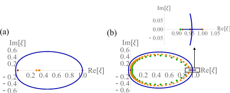
Figure 14: (a) Eigenspectrum of a quantum channel for the helical Maxwell’s demon with additional feedback performed after the second measurement. (b) Eigenspectrum of a quantum channel for the helical Maxwell’s demon with no further feedback performed after the second measurement. An enlarged eigenspectrum near the steady state is also shown. Blue curves and the blue dot at the origin constitute the eigenspectrum under the PBC, orange dots constitute the eigenspectrum under the OBC with $L=30$, and green dots constitute that under the OBC with $L=20$. The hopping amplitude is set to $J=1$ and the transverse magnetic field is set to $h_{x}=0.2$. The duration of feedback is $\tau=1$.

VII.3 QND demon

Here, we present a model of topological feedback control with strong unitary symmetry by following the construction in Sec. VI.3. We consider a spin-$1/2$ particle on a 1D lattice with two sublattices. A quantum state at site $j$ with sublattice $a=A,B$ and spin $\sigma=\uparrow,\downarrow$ is denoted by $\ket{j,a,\sigma}$. We perform a projective position measurement on this particle, and assume that this measurement does not disturb the spin state of the particle. Thus, a measurement outcome is specified only by the site index $j$ and the sublattice index $a$, and therefore the measurement operator is given by

$$\hat{M}_{j,a}=\ket{j,a,\uparrow}\bra{j,a,\uparrow}+\ket{j,a,\downarrow}\bra{j,a,\downarrow}.$$ (139)

The measurement operator satisfies $[\hat{M}_{j,a},\hat{S}^{z}]=0$, where

$$\hat{S}^{z}=\frac{1}{2}\sum_{i,a}(\ket{i,a,\uparrow}\bra{i,a,\uparrow}-\ket{i,a,\downarrow}\bra{i,a,\downarrow})$$ (140)

is the magnetization. Thus, the position measurement does not influence the spin degrees of freedom and serves as a QND measurement for $\hat{S}^{z}$ (see Sec. VI.3.1).

If the measurement outcome is $m=(j,a)$, we perform feedback control with Hamiltonian $\hat{H}_{m}$ given by

$$\hat{H}_{j,A}= -J_{1}\sum_{i,\sigma}(\ket{i,A,\sigma}\bra{i,B,\sigma}+\mathrm{H.c.})$$

$$-J_{2}\sum_{i,\sigma}(\ket{i+1,A,\sigma}\bra{i,B,\sigma}+\mathrm{H.c.})$$

$$+V\sum_{\sigma}\ket{j-1,B,\sigma}\bra{j-1,B,\sigma}$$

$$-\sum_{i}(h_{z}+h_{s})(\ket{i,A,\uparrow}\bra{i,A,\uparrow}-\ket{i,A,\downarrow}\bra{i,A,\downarrow})$$

$$-\sum_{i}(h_{z}-h_{s})(\ket{i,B,\uparrow}\bra{i,B,\uparrow}-\ket{i,B,\downarrow}\bra{i,B,\downarrow}),$$ (141)

and

$$\hat{H}_{j,B}= -J_{1}\sum_{i,\sigma}(\ket{i,A,\sigma}\bra{i,B,\sigma}+\mathrm{H.c.})$$

$$-J_{2}\sum_{i,\sigma}(\ket{i+1,A,\sigma}\bra{i,B,\sigma}+\mathrm{H.c.})$$

$$+V\sum_{\sigma}\ket{j,A,\sigma}\bra{j,A,\sigma}$$

$$-\sum_{i}(h_{z}+h_{s})(\ket{i,A,\uparrow}\bra{i,A,\uparrow}-\ket{i,A,\downarrow}\bra{i,A,\downarrow})$$

$$-\sum_{i}(h_{z}-h_{s})(\ket{i,B,\uparrow}\bra{i,B,\uparrow}-\ket{i,B,\downarrow}\bra{i,B,\downarrow}),$$ (142)

where $J_{1},J_{2}$ are the hopping amplitudes, $V$ is the height of the potential, and $h_{z}$ ($h_{s}$) denotes the strength of a uniform (staggered) magnetic field. The feedback Hamiltonian conserves the magnetization, i.e., $[\hat{H}_{m},\hat{S}^{z}]=0$. The Hamiltonians (141) and (142) are generalized versions of the chiral Maxwell’s demon discussed in Sec. IV. The CPTP map for this feedback control is given by Eq. (5) with $\hat{K}_{m}=\hat{U}_{m}\hat{M}_{m}$ and $\hat{U}_{m}=\exp[-i\hat{H}_{m}\tau]$.

Since $[\hat{M}_{m},\hat{S}^{z}]=[\hat{H}_{m},\hat{S}^{z}]=0$, the CPTP map for this feedback control has strong symmetry (see Sec. VI.3). Hence, the CPTP map can be decomposed into four parts which act on subspaces with different symmetry eigenvalues. Specifically, we have

$$\tilde{\mathcal{E}}= \sum_{m}\hat{K}_{m}\otimes\hat{K}_{m}^{*}$$

$$= \tilde{\mathcal{E}}_{\uparrow\uparrow}+\tilde{\mathcal{E}}_{\uparrow\downarrow}+\tilde{\mathcal{E}}_{\downarrow\uparrow}+\tilde{\mathcal{E}}_{\downarrow\downarrow},$$ (143)

where

$$\tilde{\mathcal{E}}_{\sigma\sigma^{\prime}}:=\sum_{j,a}\hat{U}_{j,a}\hat{M}_{j,a,\sigma}\otimes\hat{U}_{j,a}^{*}\hat{M}_{j,a,\sigma^{\prime}}^{*},$$ (144)

and

$$\hat{M}_{j,a,\sigma}:=\ket{j,a,\sigma}\bra{j,a,\sigma}.$$ (145)

In Fig. 15, we plot the eigenspectra of the quantum channel $\tilde{\mathcal{E}}$ under the PBC and the OBC together with those of $\tilde{\mathcal{E}}_{\sigma\sigma^{\prime}}$. The topological characterization of the quantum channel can be applied to each symmetry sector. The PBC eigenspectrum of $\tilde{\mathcal{E}}_{\sigma\sigma^{\prime}}$ with $\sigma=\sigma^{\prime}$ contains a single loop with winding number $-2$, while that of $\tilde{\mathcal{E}}_{\sigma\sigma^{\prime}}$ with $\sigma\neq\sigma^{\prime}$ contains two loops, each of which has winding number $-1$. Here, the uniform and staggered magnetic fields lift the degeneracy of the eigenspectra of $\tilde{\mathcal{E}}_{\sigma\sigma^{\prime}}$’s. Importantly, the eigenspactrum of $\tilde{\mathcal{E}}_{\sigma\sigma^{\prime}}$ with $\sigma\neq\sigma^{\prime}$ is no longer symmetric with respect to the real axis, implying that the modular conjugation symmetry is broken in these symmetry sectors. Thus, $\tilde{\mathcal{E}}_{\sigma\sigma^{\prime}}$ with $\sigma\neq\sigma^{\prime}$ offers a topologically nontrivial superoperator in class A.

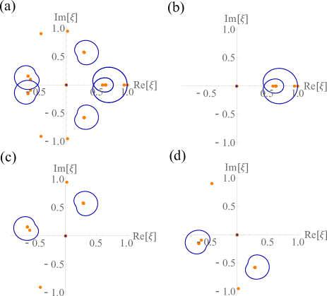
Figure 15: Eigenspectrum of a quantum channel for feedback control with strong unitary symmetry. In each figure, blue curves and the blue dot at the origin constitute the eigenspectrum under the PBC in the infinite-size limit, and orange dots constitute the eigenspectrum under the OBC with the number of unit cells $L=40$. (a) Full eigenspectrum of the CPTP map $\tilde{\mathcal{E}}$. (b) Eigenspectrum of $\tilde{\mathcal{E}}_{\uparrow\uparrow}$, which is identical to that of $\tilde{\mathcal{E}}_{\downarrow\downarrow}$. (c) Eigenspectrum of $\tilde{\mathcal{E}}_{\uparrow\downarrow}$. (d) Eigenspectrum of $\tilde{\mathcal{E}}_{\downarrow\uparrow}$. The paramaters of the model are set to $J_{1}=J_{2}=1$, $V=+\infty$, $h_{z}=0.5$, and $h_{s}=1$. The duration of feedback is $\tau=2$.

VII.4 $\mathbb{Z}_{2}$ demon

So far, we have discussed topological feedback controls in class AI, AI$+$psH_-, and A, all of which are characterized by an integer-valued winding number in 1D. In contrast, the topological classification for class AII^† implies the existence of a $\mathbb{Z}_{2}$ topological invariant in 1D [34]. Here we present topological feedback control that is characterized by a $\mathbb{Z}_{2}$ topological invariant.

As shown in Sec. VI.3.3, a quantum channel in class AII^† requires unitary symmetry and $C$ symmetry with $\eta_{C}=-1$ of the truncated Bloch matrix. To construct feedback control that fulfills these requirements, we consider a spin-$1/2$ particle on a 1D lattice with two sublattices as in Sec. VII.3. We first perform a spin-nondisturbing projective measurement of the position and the sublattice, where the measurement operator is given by Eq. (139). For a measurement outcome $m_{1}=(j_{1},a_{1})$, we perform feedback control with Hamiltonian $\hat{H}_{m_{1}}$ that has a symmetry

$$(-i\hat{\Sigma}_{y})\hat{H}_{m_{1}}^{*}(-i\hat{\Sigma}_{y})=\hat{H}_{m_{1}},$$ (146)

where

$$\hat{\Sigma}_{y}=i\sum_{j,\sigma}(\ket{j,B,\sigma}\bra{j,A,\sigma}-\ket{j,A,\sigma}\bra{j,B,\sigma}).$$ (147)

An example of such feedback Hamiltonians is given by

$$\hat{H}_{j_{1},A}= -J_{1}\sum_{a=A,B}\sum_{\sigma=\uparrow,\downarrow}(\ket{j_{1},a,\sigma}\bra{j_{1}-1,a,\sigma}+\mathrm{H.c.})-J_{2}\sum_{a}\sum_{\sigma}(\ket{j_{1}+1,a,\sigma}\bra{j_{1},a,\sigma}+\mathrm{H.c.})$$

$$+\lambda\sum_{\sigma}(\ket{j_{1},B,\sigma}\bra{j_{1}-1,A,\sigma}+\ket{j_{1}+1,B,\sigma}\bra{j_{1},A,\sigma}-\ket{j_{1},A,\sigma}\bra{j_{1}-1,B,\sigma}-\ket{j_{1}+1,A,\sigma}\bra{j_{1},B,\sigma}+\mathrm{H.c.}),$$ (148)

and

$$\hat{H}_{j_{1},B}= -J_{2}\sum_{a=A,B}\sum_{\sigma=\uparrow,\downarrow}(\ket{j_{1},a,\sigma}\bra{j_{1}-1,a,\sigma}+\mathrm{H.c.})-J_{1}\sum_{a}\sum_{\sigma}(\ket{j_{1}+1,a,\sigma}\bra{j_{1},a,\sigma}+\mathrm{H.c.})$$

$$+\lambda\sum_{\sigma}(\ket{j_{1},B,\sigma}\bra{j_{1}-1,A,\sigma}+\ket{j_{1}+1,B,\sigma}\bra{j_{1},A,\sigma}-\ket{j_{1},A,\sigma}\bra{j_{1}-1,B,\sigma}-\ket{j_{1}+1,A,\sigma}\bra{j_{1},B,\sigma}+\mathrm{H.c.}),$$ (149)

which are schematically illustrated in Fig. 16. For computational simplicity, here we assume that $\hat{H}_{j_{1},a}$ acts only on three unit cells labeled by $j_{1}-1,j_{1},j+1$; however, this assumption is not essential. After the unitary time evolution described by $\hat{U}_{j_{1},a_{1}}=\exp[-i\hat{H}_{j_{1},a_{1}}\tau]$, we perform the second projective measurement of the position and the sublattice with the same measurement operators (139) and suppose that we obtain an outcome $m_{2}=(j_{2},a_{2})$. Then, using the set of measurement outcomes $m_{1}$ and $m_{2}$, we perform additional feedback control with the following unitary operator:

$$\hat{U}_{m_{1},m_{2}}^{\prime}=\begin{cases}\exp[-i\pi\hat{S}^{z}]&(j_{1}>j_{2}\ \mathrm{and}\ a_{1}\neq a_{2});\\ \hat{I}&(\mathrm{otherwise}).\end{cases}$$ (150)

This addtional feedback control can be realized by a magnetic field and imprints a phase depending on the spin degrees of freedom. This feedback control is essential for realizing $C$ symmetry of a quantum channel (see below).

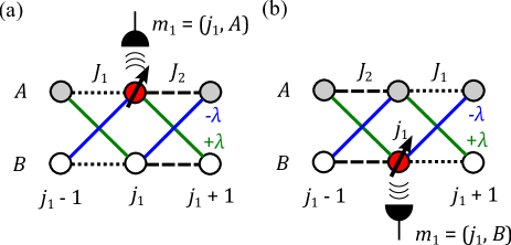
Figure 16: Schematic illustration of the $\mathbb{Z}_{2}$ demon. We first perform a projective measurement of the position and the sublattice without disturbing the spin degrees of freedom. (a) If a particle is detected at site $j_{1}$ and sublattice $A$, we perform feedback control by using the Hamiltonian $H_{j_{1},A}$. (b) If a particle is detected at site $j_{1}$ and sublattice $B$, we perform feedback control by using the Hamiltonian $H_{j_{1},B}$. After the unitary evolution under the feedback Hamiltonian $H_{j_{1},a_{1}}$ $(a_{1}=A,B)$, we perform the second projective measurement and additional feedback with a magnetic field [see Eq. (150)].

The quantum channel for the entire process is given by

$$\tilde{\mathcal{E}}= \sum_{m_{1},m_{2}}\hat{K}_{m_{1},m_{2}}\otimes\hat{K}_{m_{1},m_{2}}^{*}$$

$$= \tilde{\mathcal{E}}_{\uparrow\uparrow}+\tilde{\mathcal{E}}_{\uparrow\downarrow}+\tilde{\mathcal{E}}_{\downarrow\uparrow}+\tilde{\mathcal{E}}_{\downarrow\downarrow},$$ (151)

where $\hat{K}_{m_{1},m_{2}}=\hat{U}_{m_{1},m_{2}}^{\prime}\hat{M}_{m_{2}}\hat{U}_{m_{1}}\hat{M}_{m_{1}}$ is the Kraus operator and

$$\tilde{\mathcal{E}}_{\sigma\sigma^{\prime}}= U_{m_{1},m_{2}}^{\prime}\hat{M}_{j_{2},a_{2},\sigma}\hat{U}_{m_{1}}\hat{M}_{j_{1},a_{1},\sigma}$$

$$\otimes(\hat{U}_{m_{1},m_{2}}^{\prime}\hat{M}_{j_{2},a_{2},\sigma^{\prime}}\hat{U}_{m_{1}}\hat{M}_{j_{1},a_{1},\sigma^{\prime}})^{*}$$ (152)

with Eq. (145). The decomposition of $\tilde{\mathcal{E}}$ into $\tilde{\mathcal{E}}_{\sigma\sigma^{\prime}}$’s is due to the conservation of $\hat{S}^{z}$ during the measurement and feedback processes (i.e., strong symmetry).

From the general discussion presented in Sec. VI.3, the truncated Bloch matrix $X_{\mathrm{trunc}}^{(\sigma\sigma^{\prime})}(k)$ is given by Eq. (98) with Eq. (99); however, because of the additional feedback, Eq. (100) is changed to

$$q^{(\sigma\sigma^{\prime})}(j_{2},a_{2}|j_{1},a_{1})= \mathrm{sgn}[\sigma\sigma^{\prime}]^{\theta(j_{1}-j_{2}-1/2)}$$

$$\times(\hat{U}_{j_{1},a_{1}}) {}_{j_{2},a_{2},\sigma;j_{1},a_{1},\sigma}(\hat{U}_{j_{1},a_{1}})_{j_{2},a_{2},\sigma^{\prime};j_{1},a_{1},\sigma^{\prime}}^{*},$$ (153)

for $a_{1}\neq a_{2}$, where $\theta(x)$ is the Heaviside unit-step function and

$$\mathrm{sgn}[\sigma\sigma^{\prime}]:=\begin{cases}1&(\sigma=\sigma^{\prime});\\ -1&(\sigma\neq\sigma^{\prime}).\end{cases}$$ (154)

The unitary operator with the feedback Hamiltonian $H_{m_{1}}$ statisfies the following reciprocity relations because of the symmetry between $\hat{H}_{j_{1},A}$ and $\hat{H}_{j_{1},B}$:

$$(\hat{U}_{j_{1},A})_{j_{2},A,\sigma;j_{1},A,\sigma}(\hat{U}_{j_{1},A})_{j_{2},A,\sigma^{\prime};j_{1},A,\sigma^{\prime}}^{*}$$

$$=(\hat{U}_{j_{2},B})_{j_{1},B,\sigma;j_{2},B,\sigma}(\hat{U}_{j_{2},B})_{j_{1},B,\sigma^{\prime};j_{2},B,\sigma^{\prime}}^{*},$$ (155a)

$$(\hat{U}_{j_{1},B})_{j_{2},A,\sigma;j_{1},B,\sigma}(\hat{U}_{j_{1},B})_{j_{2},A,\sigma^{\prime};j_{1},B,\sigma^{\prime}}^{*}$$

$$=(\hat{U}_{j_{2},B})_{j_{1},A,\sigma;j_{2},B,\sigma}(\hat{U}_{j_{2},B})_{j_{1},A,\sigma^{\prime};j_{2},B,\sigma^{\prime}}^{*},$$ (155b)

$$(\hat{U}_{j_{1},A})_{j_{2},B,\sigma;j_{1},A,\sigma}(\hat{U}_{j_{1},A})_{j_{2},B,\sigma^{\prime};j_{1},A,\sigma^{\prime}}^{*}$$

$$=(\hat{U}_{j_{2},A})_{j_{1},B,\sigma;j_{2},A,\sigma}(\hat{U}_{j_{2},A})_{j_{1},B,\sigma^{\prime};j_{2},A,\sigma^{\prime}}^{*}.$$ (155c)

In addition, we have

$$q^{(\sigma\sigma^{\prime})}(j,A|j,B)=q^{(\sigma\sigma^{\prime})}(j,B|j,A)=0$$ (156)

from the symmetry of the unitary operator

$$(-i\hat{\Sigma}_{y})\hat{U}_{m_{1}}^{T}(-i\hat{\Sigma}_{y})^{-1}=\hat{U}_{m_{1}},$$ (157)

which follows from the symmetry (146) of the feedback Hamiltonian. Then, the conditions (106a)-(106c) are satisfied, and thus $\tilde{\mathcal{E}}_{\sigma\sigma^{\prime}}$ with $\sigma\neq\sigma^{\prime}$ belongs to class AII^†, while that with $\sigma=\sigma^{\prime}$ belongs to class AI$+$psH₊.

The topological feedback control in class AII^† exhibits the $\mathbb{Z}_{2}$ skin effect [72]. To see this, we show the eigenspectrum of the quantum channel for the $\mathbb{Z}_{2}$ demon under the PBC and the OBC in Fig. 17. The block-diagonalized CPTP map $\tilde{\mathcal{E}}_{\uparrow\uparrow}$ does not possess $C$ symmetry with $\eta_{C}=-1$, and therefore the Kramers degeneracy of eigenvalues is not ensured. Consequently, the loop structure in the eigenspectrum of $\tilde{\mathcal{E}}_{\uparrow\uparrow}$ shown in Fig. 17(a) collapses near the real axis due to real-complex transitions and does not support nontrivial topology. In contrast, the block $\tilde{\mathcal{E}}_{\uparrow\downarrow}$ has $C$ symmetry with $\eta_{C}=-1$, leading to a Kramers-degenerated eigenspectrum shown in Fig. 17(b). The point-gap topology of this spectrum is characterized by a $\mathbb{Z}_{2}$ topological invariant [72]

$$(-1)^{\nu(\xi_{\mathrm{PG}})}= \mathrm{sgn}\Biggl{\{}\frac{\mathrm{Pf}[(X_{\mathrm{trunc}}^{(\uparrow\downarrow)}(\pi)-\xi_{\mathrm{PG}})(-i\sigma_{y})]}{\mathrm{Pf}[(X_{\mathrm{trunc}}^{(\uparrow\downarrow)}(0)-\xi_{\mathrm{PG}})(-i\sigma_{y})]}$$

$$\times\exp\Bigl{[}-\frac{1}{2} \int_{k=0}^{k=\pi}d\log\det\{(X_{\mathrm{trunc}}^{(\uparrow\downarrow)}(k)-\xi_{\mathrm{PG}})(-i\sigma_{y})\}\Bigr{]}\Biggr{\}}.$$ (158)

Indeed, the eigenspectrum of $\tilde{\mathcal{E}}_{\uparrow\downarrow}$ under the OBC forms a line rather than a closed loop, which is a hallmark of the $\mathbb{Z}_{2}$ skin effect. Interestingly, the $\mathbb{Z}_{2}$ skin effect can occur only in $\tilde{\mathcal{E}}_{\sigma\sigma^{\prime}}$ with $\sigma\neq\sigma^{\prime}$ since $\tilde{\mathcal{E}}_{\sigma\sigma}$ has the modular conjugation symmetry and is therfore characterized by the winding number rather than the $\mathbb{Z}_{2}$ invariant (see Sec. VII.2). Physically, the eigenspectra in Fig. 17 indicate that off-diagonal elements of the density matrix in terms of the $\hat{S}^{z}$ basis are accumulated on the edges of the system, whereas diagonal elements are delocalized over the system. Such distinct behavior is induced by the additional feedback in Eq. (150), which nontrivially acts only on the off-diagonal elements.

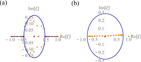
Figure 17: Eigenspectrum of a quantum channel for the $\mathbb{Z}_{2}$ demon. In each figure, blue curves and the blue dot at the origin constitute the eigenspectrum under the PBC in the infinite-size limit, and orange dots constitute the eigenspectrum under the OBC with the number of unit cells $L=20$. (a) Eigenspectrum of $\tilde{\mathcal{E}}_{\uparrow\uparrow}$. (b) Eigenspectrum of $\tilde{\mathcal{E}}_{\uparrow\downarrow}$. The paramaters of the model are set to $J_{1}=0.8,J_{2}=1$ and, $\lambda=0.5$. The duration of feedback is $\tau=1$.

Here we remark on the boundary condition of the $\mathbb{Z}_{2}$ demon. To see the non-Hermitian skin effect in symmetry-protected topological feedback control, a quantum channel under the OBC must respect the protecting symmetry. We detail how to implement a symmetry-preserving OBC in Appendix E.

VIII Dissipative feedback control

VIII.1 Formalism

In reality, there exist many sources of noise and dissipation during feedback control. The formalism presented so far can be generalized to such cases in which feedback operations are not unitary. Suppose that a feedback operation depending on a measurement outcome $m$ is described by a CPTP map

$$\mathcal{F}_{m}(\hat{\rho})=\sum_{\alpha}\hat{F}_{m,\alpha}\hat{\rho}\hat{F}_{m,\alpha}^{\dagger},$$ (159)

where the Kraus operators $\hat{F}_{m,\alpha}$ satisfy

$$\sum_{\alpha}\hat{F}_{m,\alpha}^{\dagger}\hat{F}_{m,\alpha}=\hat{I}.$$ (160)

Then, given an initial density matrix $\hat{\rho}_{\mathrm{i}}$, the density matrix after feedback control is given by

$$\hat{\rho}_{\mathrm{f}}= \sum_{m}p_{m}\mathcal{F}_{m}\Bigl{(}\frac{1}{p_{m}}\hat{M}_{m}\hat{\rho}_{\mathrm{i}}\hat{M}_{m}^{\dagger}\Bigr{)}$$

$$= \sum_{m}\sum_{\alpha}\hat{F}_{m,\alpha}\hat{M}_{m}\hat{\rho}_{\mathrm{i}}\hat{M}_{m}^{\dagger}\hat{F}_{m,\alpha}^{\dagger},$$ (161)

where $p_{m}=\mathrm{Tr}[\hat{M}_{m}^{\dagger}\hat{M}_{m}\hat{\rho}_{\mathrm{i}}]$ is the probability of outcome $m$ for the measurement operator $\hat{M}_{m}$. Thus, the feedback control is described by a quantum channel

$$\mathcal{E}(\hat{\rho})=\sum_{m,\alpha}\hat{K}_{m,\alpha}\hat{\rho}\hat{K}_{m,\alpha}^{\dagger}$$ (162)

with Kraus operators

$$\hat{K}_{m,\alpha}:=\hat{F}_{m,\alpha}\hat{M}_{m}.$$ (163)

Note that

$$\sum_{m,\alpha}\hat{K}_{m,\alpha}^{\dagger}\hat{K}_{m,\alpha}= \sum_{m,\alpha}\hat{M}_{m}^{\dagger}\hat{F}_{m,\alpha}^{\dagger}\hat{F}_{m,\alpha}\hat{M}_{m}$$

$$= \sum_{m}\hat{M}_{m}^{\dagger}\hat{M}_{m}=\hat{I}$$ (164)

holds due to Eq. (160) and $\sum_{m}\hat{M}_{m}^{\dagger}\hat{M}_{m}=\hat{I}$.

By repeating the analysis in Sec. III.1 for the quantum channel (162), the eigenspectrum of the quantum channel is given by that of the Bloch matrix $X(\vec{k})$, whose matrix elements are given by

$$X_{a,c,\vec{\mu};b,d,\vec{\nu}}(\vec{k}):= \frac{1}{N_{\mathrm{cell}}}\sum_{\vec{j},\vec{j}^{\prime}}\sum_{m,\alpha}(\hat{K}_{m,\alpha})_{\vec{j},a;\vec{j}^{\prime},b}$$

$$\times(\hat{K}_{m,\alpha})^{*}_{\vec{j}+\vec{\mu},c;\vec{j}^{\prime}+\vec{\nu},d}e^{-i\vec{k}\cdot(\vec{R}_{\vec{j}}-\vec{R}_{\vec{j}^{\prime}})}.$$ (165)

The difference from the case with unitary feedback is the exitense of the additional index $\alpha$, which can be regarded as information that cannot be specified in the feedback process.

VIII.2 Dissipative Maxwell’s demon

As an example of dissipative feedback control described by a CPTP map (159), we consider a chiral Maxwell’s demon (see Sec. IV) subject to dissipation. We consider a spinless particle on a 1D lattice with $L$ sites, and perform projective position measurement for this particle as in Sec. IV. We then perform a feedback operation governed by the Lindblad equation

$$\frac{d\hat{\rho}}{dt}= \mathcal{L}_{m}(\hat{\rho})$$

$$= -i[\hat{H}_{m},\hat{\rho}]+\sum_{j}\Bigl{(}\hat{L}_{m,j}\hat{\rho}\hat{L}_{m,j}^{\dagger}-\frac{1}{2}\{\hat{L}_{m,j}^{\dagger}\hat{L}_{m,j},\hat{\rho}\}\Bigr{)},$$ (166)

where $\mathcal{L}_{m}$ is the generator (Lindbladian) conditioned on the measurement outcome, $H_{m}$ is a feedback Hamiltonian given in Sec. IV, and $\hat{L}_{m,j}$ is the Lindblad operator acting on a local region around site $j$. Then, a CPTP map for the feedback operation is given by

$$\mathcal{F}_{m}=e^{\mathcal{L}_{m}\tau},$$ (167)

where $\tau$ is the duration of feedback. Using the Lindblad equation (166), we can consider various dissipative effects on feedback control such as noise during feedback and a coupling to a reservoir. In particular, if the system is in contact with a heat bath, the topological Maxwell’s demon can rectify thermal fluctuations as well as quantum fluctuations to achieve unidirectional transport of a particle. However, we note that the Hamiltonian and the Lindblad operators in Eq. (166) should be chosen to be local to ensure the locality of the Kraus operators and to allow truncation of the Bloch matrix into a finite-dimensional matrix (see Sec. III.2). The locality-preserving Lindblad equation can be derived if the correlation time of the environment is sufficiently short [99].

Since the matrix elements of the Kraus operator $\hat{K}_{m,\alpha}=\hat{F}_{m,\alpha}\hat{M}_{m}$ are written as

$$(\hat{K}_{m,\alpha})_{i,j}=(\hat{F}_{m,\alpha}\hat{M}_{m})_{i,j}=(\hat{F}_{m,\alpha})_{i,m}\delta_{j,m},$$ (168)

the Bloch matrix of the quantun channel is given by

$$X_{\mu,\nu}(k)= \frac{1}{L}\sum_{j,j^{\prime}}\sum_{m,\alpha}(\hat{K}_{m,\alpha})_{j,j^{\prime}}(\hat{K}_{m,\alpha})^{*}_{j+\mu,j^{\prime}+\nu}e^{-ik(j-j^{\prime})}$$

$$= \delta_{\nu,0}\frac{1}{L}\sum_{j}\sum_{m,\alpha}(\hat{F}_{m,\alpha})_{j,m}(\hat{F}_{m,\alpha})^{*}_{j+\mu,m}e^{-ik(j-m)}.$$ (169)

Thus, similarly to the case with unitary feedback control, eigenvalues of the Bloch matrix are given by

$$\xi_{0}(k)= X_{0,0}(k)$$

$$= \frac{1}{L}\sum_{j}\sum_{m,\alpha}|(\hat{F}_{m,\alpha})_{j,m}|^{2}e^{-ik(j-m)},$$ (170)

$$\xi_{1}(k)= \xi_{2}(k)=\cdots=\xi_{L-1}(k)=0.$$ (171)

Here we note that

$$\sum_{\alpha}|(\hat{F}_{m,\alpha})_{j,m}|^{2}= \sum_{\alpha}\bra{j}\hat{F}_{m,\alpha}\ket{m}\bra{m}\hat{F}_{m,\alpha}^{\dagger}\ket{j}$$

$$= \bra{j}\mathcal{F}_{m}(\ket{m}\bra{m})\ket{j}$$

$$= \bra{j}\mathcal{F}_{m}\Bigl{(}\frac{1}{p_{m}}\hat{M}_{m}\hat{\rho}\hat{M}_{m}^{\dagger}\Bigr{)}\ket{j}$$

$$= p(j|m),$$ (172)

where $p(j|m)$ is the probability of a particle being found at site $j$ after the feedback control with outcome $m$. Then, the eigenvalue $\xi_{0}(k)$ is written as

$$\xi_{0}(k)= \frac{1}{L}\sum_{j,m}p(j|m)e^{-ik(j-m)},$$ (173)

which takes the same form as in the case with unitary feedback control [see Eq. (43)]. Thus, regardless of whether the feedback control is unitary or not, the eigenvalue of the quantum channel and its topology are completely determined from the probability distribution $p(j|m)$ of the position after the feedback.

To demonstrate the robustness of the chiral Maxwell’s demon against dissipation during feedback control, we consider the Lindblad operators

$$L_{m,j}^{(\mathrm{d})}= \sqrt{\gamma_{\mathrm{d}}}\ket{j}\bra{j},$$ (174)

$$L_{m,j}^{(\mathrm{L})}= \sqrt{\gamma_{\mathrm{L}}}\ket{j-1}\bra{j},$$ (175)

$$L_{m,j}^{(\mathrm{R})}= \sqrt{\gamma_{\mathrm{R}}}\ket{j+1}\bra{j}.$$ (176)

which respectively describe dephasing, stochastic hopping to the left direction, and stochastic hopping to the right direction [see Fig. 18(a) for a schematic illustration]. Figure 18(b) shows the eigenspectrum of the quantum channel for the chiral Maxwell’s demon subject to dissipation. As can be seen from the figure, the loop structure of the eigenspectrum under the PBC is robust against dissipation, leading to the non-Hermitian skin effect under the OBC. This result indicates that the chiral Maxwell’s demon can rectify the noise induced by dissipation as well as quantum fluctuations induced by unitary evolution, and achieve unidirectional transport that is robust against noise and decoherence.

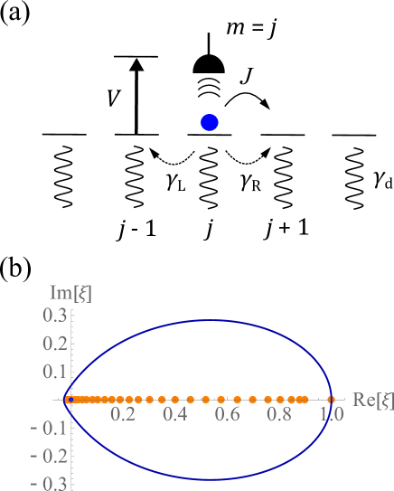
Figure 18: (a) Schematic illustration of a chiral Maxwell’s demon subject to dissipation. (b) Eigenspectrum of a quantum channel for a chiral Maxwell’s demon subject to dissipation. The parameters are set to be $J=1,V=10,\gamma_{\mathrm{d}}=0.5,\gamma_{\mathrm{L}}=\gamma_{\mathrm{R}}=0.25$, and $\tau=1$. A blue curve and blue dots at the origin constitute the eigenspectrum under the PBC in the limit of infinite system size, and orange dots show the eigenspectrum under the OBC with the system size $L=30$.

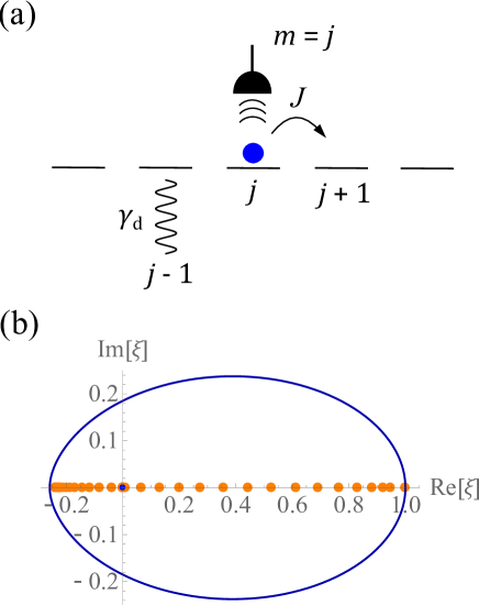
Figure 19: (a) Schematic illustration of topological feedback control with engineered dissipation. (b) Eigenspectrum of a quantum channel for topological feedback control with engineered dissipation. The parameters are set to be $J=1,\gamma_{\mathrm{d}}=5$, and $\tau=1$. A blue curve and blue dots at the origin constitue the eigenspectrum under the PBC in the limit of infinite system size, and orange dots show the eigenspectrum under the OBC with the system size $L=30$.

VIII.3 Feedback control with engineered dissipation

Dissipative feedback control not only shows the stability of topological feedback control against noise, but also can be exploited to utilize dissipation as an essential tool for feedback control. Such a possibility can be envisaged since recent developments in quantum technologies with atoms, ions, and photons have enabled one to realize engineered dissipation [100]. For example, localized dissipation can be introduced in ultracold atoms, where the strength of dissipation is controlled by laser fields [101, 102, 103, 104, 105]. Motivated by the possibility of dissipation engineering, we propose a topological feedback control that is enabled by dissipation.

The setup of feedback control with engineered dissipation is as follows. We consider a spinless particle on a 1D lattice, perform projective position measurement on it, and obtain a measurement outcome $m$. Then, we let the particle undergo dissipative time evolution under the Lindblad equation (166). Here, we assume that the Hamiltonian does not depend on the measurement outcome $m$ and is given by a simple tight-binding model

$$H_{m}=H:=-J\sum_{j}(\ket{j}\bra{j+1}+\mathrm{H.c.})$$ (177)

with $J>0$ being the hopping amplitude. The dependence of the conditioned Lindblad equation (166) on the measurement outcome is encoded in the Lindblad operator, where engineered disipation is described by

$$L_{m,j-1}=\delta_{m,j}\sqrt{\gamma_{\mathrm{d}}}\ket{j-1}\bra{j-1}.$$ (178)

In other words, we introduce localized dissipation to the left site of the particle [see Fig. 19(a) for a schematic illustration]. Here we exploit the continuous quantum Zeno effect [106] in the strong-dissipation regime $\gamma_{\mathrm{d}}\gg J$ to suppress the hopping of the particle to the site that is subject to strong dissipation. Because of this feedback control of dissipation, hopping of a particle to the right is facilitated and chiral transport is eventually achieved.

The eigenspectrum of a quantum channel for this dissipative feedback control is shown in Fig. 19(b). The eigenspectrum under the PBC forms a loop and that under the OBC displays the non-Hermitian skin effect. Here, the loop structure of the eigenspectrum under the PBC is realized due to the dissipation, since the Hamiltonian (177) does not contain a wall potential. Thus, the topological feedback control, and the associated chiral transport, are achieved by dissipation.

IX Conclusion and outlook

In summary, we have presented a class of dynamical topological phases realized with feedback control, which are chracterized by topology of quantum channels. The nontrivial point-gap topology of a quantum channel chracterized by a winding number ensures robust chiral tranport, which is analogous to the chiral edge current in the quantum Hall effect, and leads to the emergence of the non-Hermitian skin effect under the open boundary condition. We have also provided a symmetry classification of quantum feedback control, identified ten classes compatible with projective measurement, and constructed examples of feedback control in each symmetry class. This general framework of symmetry and topology of quantum feedback control provides a guiding princple for designing stable feedback control of quantum systems since topology is insensitive to small deformation. Also, feedback control offers a unique way of control of dynamical topological phases of matter distinct from other well-known classes such as periodically driven systems [20, 21, 22, 23, 24, 25, 26, 27, 28, 29, 30, 31], non-Hermitian systems [32, 33, 34, 35, 36, 37, 38], and open quantum systems subject to engineered dissipation [64, 65].

Topological feedback control is expected to be realized in various experimental platforms. For example, the past decade has witnessed remarkable progress in site-resolved measurement techniques and control of ultracold atoms in optical lattices [107, 108, 109]. More recently, atoms in optical tweezer arrays have emerged as a highly-controllable quantum simulator in which individual atoms can be measured and addressed in a programmable manner [110, 111, 112, 113, 114, 50, 115]. The high-precision position measurement and subsequent local control of a Hamiltonian for topological feedback control can be achieved by these state-of-the-art techniques. In addition to these promising platforms, quantum feedback control has widely been used in photonic systems [42, 58], levitated nanoparticles [44, 45, 46], and superconducting qubits [43, 60, 61, 62]. Given the rapid development in quantum control, topological feedback control in various experimental platforms will expand the scope of topological phases of matter.

We conclude this paper by discussing future perspectives and open problems. First, while we have focused on point-gap topology of quantum channels, line-gap topology remains to be investigated. In analogy with dissipative topological insulators [34], nontrivial line-gap topology of quantum channels may lead to boundary-localized states and it can therefore be used to create and stabilize topological boundary states with feedback control.

Second, while we have mostly focused on feedback control with projective measurement, the present framework for topology of quantum channels is also applicable to general quantum measurement, and therefore it is natural to ask whether non-projective measurement can be harnessed to construct topological feedback control. In particular, since the symmetry classification in Sec. V.3 is based on the spectral property of projective measurement channels, BL symmetry classes other than those in Table 2 are not prohibited for general quantum measurement. Since a quantum channel in a symmetry class beyond the ten-fold way necessarily has a pair of eigenvalues $\pm 1$ (if one assumes the existense of a steady state), its eigenvalue spectrum is reminiscent of that of dissipative time crystals [33, 116], where the eigenvalue $-1$ implies oscillating components under repeated application of a quantum channel.

Third, a crucial distinction between quantum channels and general non-Hermitian matrices is complete positivity and trace preservation (CPTP), which should be satisfied by any time evolution of the density matrix of a quantum system [47]. Although the topological classification of non-Hermitian matrices without the CPTP condition has been obtained [34, 35], it is unclear whether the CPTP condition alters the topological classification. For example, in Sec. VI.2, we have shown that the CPTP condition places a nontrivial constraint on the Bloch matrix with transposition symmetry, which turns out to be characterized by an integer topological invariant rather than a $\mathbb{Z}_{2}$ invariant. It merits further study to investigate the generality of this phenomenon. From a broader perspective, this problem may be related to a classification of time evolution of open quantum systems described by CPTP maps.

Last but not least, topological feedback control suggests a novel connection between topology and Maxwell’s demon. For example, an experimental realization of Maxwell’s demon in Ref. [54] demonstrated chiral transport of a particle due to feedback control, in close analogy with the chiral Maxwell’s demon in Sec. IV (see also Ref. [82]). Maxwell’s demon has been of long-standing interest in thermodynamics and statistical physics, and an information-theoretic understanding of the role of Maxwell’s demon has led to the integration of thermodynamics and information theory [53]. Investigating topology of feedback control may thus shed light on a hitherto unnoticed role of topology in thermodynamics.

Appendix A Bloch theory of quantum channels

The Bloch theory lies at the heart of topological band theory [1]. However, how to generalize it to feedback-controlled quantum systems is nontrivial since feedback control involves not only unitary time evolution but also measurement processes. Here, we develop a Bloch theory of quantum channels described by CPTP maps. The following formalism is not limited to discrete quantum feedback control but can generally be applied to any translationally invariant quantum channels in single-particle systems.

A.1 CPTP map as a non-Hermitian operator

We begin with representing a CPTP map in terms of a non-Hermitian matrix. We consider a single-particle quantum system on a lattice (see Sec. III.1 for details). We first vectorize the density matrix

$$\hat{\rho}=\sum_{\vec{i},\vec{j}}\sum_{a,b}\rho_{\vec{i},a;\vec{j},b}\ket{\vec{i},a}\bra{\vec{j},b}$$ (179)

by using the Choi-Jamiołkowski isomorphism [77, 78, 79, 80] as

$$\ket{\hat{\rho}}:= (\hat{\rho}\otimes\hat{I})\sqrt{D}\ket{\Omega}$$

$$= \sum_{\vec{i},\vec{j}}\sum_{a,b}\rho_{\vec{i},a;\vec{j},b}\ket{\vec{i},a}\otimes\ket{\vec{j},b},$$ (180)

where $\{\ket{\vec{i},a}\}$ is an orthonormal basis set of the $D$-dimensional Hilbert space $\mathcal{H}$ of a single-particle system on a lattice ($D=N_{\mathrm{cell}}D_{\mathrm{loc}}$; see Sec. III.1), and

$$\ket{\Omega}=\frac{1}{\sqrt{D}}\sum_{\vec{i}}\sum_{a}\ket{\vec{i},a}\otimes\ket{\vec{i},a}$$ (181)

is a maximally entangled state on a doubled Hilbert space $\mathcal{H}\otimes\mathcal{H}$. Consequently, we obtain a mapping from a CPTP map

$$\mathcal{E}(\hat{\rho})=\sum_{m}\hat{K}_{m}\hat{\rho}\hat{K}_{m}^{\dagger}$$ (182)

to a non-Hermitian operator $\tilde{\mathcal{E}}$ acting on $\mathcal{H}\otimes\mathcal{H}$ as

$$\tilde{\mathcal{E}}\ket{\hat{\rho}}:= \ket{\mathcal{E}(\hat{\rho})}$$

$$= (\mathcal{E}(\hat{\rho})\otimes\hat{I})\sqrt{D}\ket{\Omega}$$

$$= \sum_{m}\sum_{\vec{i},\vec{j},\vec{l}}\sum_{a,b,c}\rho_{\vec{i},a;\vec{j},b}\hat{K}_{m}\ket{\vec{i},a}\bra{\vec{j},b}\hat{K}_{m}^{\dagger}\ket{\vec{l},c}\otimes\ket{\vec{l},c}$$

$$= \sum_{m}\sum_{\vec{i},\vec{j}}\sum_{a,b}\rho_{\vec{i},a;\vec{j},b}\hat{K}_{m}\ket{\vec{i},a}\otimes\hat{K}_{m}^{*}\ket{\vec{j},b}$$

$$= \Bigl{(}\sum_{m}\hat{K}_{m}\otimes\hat{K}_{m}^{*}\Bigr{)}\ket{\hat{\rho}}.$$ (183)

Namely, we have the matrix representation of $\mathcal{E}$ as

$$\tilde{\mathcal{E}}=\sum_{m}\hat{K}_{m}\otimes\hat{K}_{m}^{*}.$$ (184)

The eigenvalues of $\tilde{\mathcal{E}}$ are the same as those of $\mathcal{E}$ since

$$\tilde{\mathcal{E}}\ket{\hat{\rho}_{n}^{R}}= \ket{\mathcal{E}(\hat{\rho}_{n}^{R})}$$

$$= \ket{\xi_{n}\hat{\rho}_{n}^{R}}$$

$$= \xi_{n}\ket{\hat{\rho}_{n}^{R}},$$ (185)

where we use Eq. (180) in deriving the last equality.

A.2 Momentum-space representation

Here we consider a translationally invariant quantum channel satisfying

$$\sum_{m}(\hat{T}_{\lambda}\hat{K}_{m}\hat{T}_{\lambda}^{-1})\hat{\rho}(\hat{T}_{\lambda}\hat{K}_{m}\hat{T}_{\lambda}^{-1})^{\dagger}=\sum_{m}\hat{K}_{m}\hat{\rho}\hat{K}_{m}^{\dagger}$$ (186)

for arbitrary $\hat{\rho}$ with $\hat{T}_{\lambda}\ (\lambda=1,\cdots,d)$ being translation operators:

$$\hat{T}_{\lambda}\ket{\vec{i},a}=\ket{\vec{i}+\vec{e}_{\lambda},a}.$$ (187)

In the matrix representation $\tilde{\mathcal{E}}$ of the CPTP map, the translational symmetry in Eq. (186) reads

$$(\hat{T}_{\lambda}\otimes\hat{T}_{\lambda}^{*})\tilde{\mathcal{E}}(\hat{T}_{\lambda}\otimes\hat{T}_{\lambda}^{*})^{-1}=\tilde{\mathcal{E}}.$$ (188)

In the context of open quantum systems, this symmetry can be regarded as weak symmetry of the CPTP map (see Sec. V.1) [90, 91]. In fact, since the operator $\tilde{\mathcal{E}}$ commutes with the tensor-product translation operator $\hat{T}_{\lambda}\otimes\hat{T}_{\lambda}^{*}$ appearing in Eq. (188), the operator $\tilde{\mathcal{E}}$ can be block-diagonalized with respect to eigenvalues of $\hat{T}_{\lambda}\otimes\hat{T}_{\lambda}^{*}$. Eigenvectors of $\hat{T}_{\lambda}\otimes\hat{T}_{\lambda}^{*}$ are constructed from the eigenstates

$$\ket{\vec{k},a}=\frac{1}{\sqrt{N_{\mathrm{cell}}}}\sum_{\vec{j}}e^{i\vec{k}\cdot\vec{R}_{\vec{j}}}\ket{\vec{j},a}$$ (189)

of the translation operator $\hat{T}_{\lambda}$ with eigenvalue $e^{-i\vec{k}\cdot\vec{a}_{\lambda}}$ as

$$(\hat{T}_{\lambda}\otimes\hat{T}_{\lambda}^{*})\ket{\vec{k},a}\otimes\ket{-\vec{k}^{\prime},b}=e^{-i(\vec{k}-\vec{k}^{\prime})\cdot\vec{a}_{\lambda}}\ket{\vec{k},a}\otimes\ket{-\vec{k}^{\prime},b}.$$ (190)

Thus, eigenvectors of $\tilde{\mathcal{E}}$ are classified according to the eigenvalues of $\hat{T}_{\lambda}\otimes\hat{T}_{\lambda}^{*}$. Since the vector $\ket{\vec{k},a}\otimes\ket{-\vec{k}^{\prime},b}$ corresponds to an operator $\ket{\vec{k},a}\bra{\vec{k}^{\prime},b}$ through the Choi-Jamiołkowski isomorphism (see Eqs. (179) and (180)), $\vec{k}-\vec{k}^{\prime}$ in Eq. (190) is physically interpreted as the difference between crystal momenta of the ket and bra degrees of freedom of the density matrix.

By using the expression of the Kraus operator

$$\hat{K}_{m}=\sum_{\vec{i},\vec{j}}\sum_{a,b}(\hat{K}_{m})_{\vec{i},a;\vec{j},b}\ket{\vec{i},a}\bra{\vec{j},b},$$ (191)

the matrix representation $\tilde{\mathcal{E}}$ of the CPTP map is written as

$$\tilde{\mathcal{E}}= \sum_{m}\hat{K}_{m}\otimes\hat{K}_{m}^{*}$$

$$= \sum_{m}\sum_{\vec{i},\vec{j},\vec{i}^{\prime},\vec{j}^{\prime}}\sum_{a,b,c,d}(\hat{K}_{m})_{\vec{i},a;\vec{j},b}(\hat{K}_{m})^{*}_{\vec{i}^{\prime},c;\vec{j}^{\prime},d}$$

$$\times\ket{\vec{i},a}\bra{\vec{j},b}\otimes\ket{\vec{i}^{\prime},c}\bra{\vec{j}^{\prime},d}$$

$$= \sum_{\vec{i},\vec{j}}\sum_{a,b,c,d}\sum_{\vec{\mu},\vec{\nu}}t_{\vec{i},\vec{j}}^{a,c,\vec{\mu};b,d,\vec{\nu}}$$

$$\times\ket{\vec{i},a}\bra{\vec{j},b}\otimes\ket{\vec{i}+\vec{\mu},c}\bra{\vec{j}+\vec{\nu},d},$$ (192)

where

$$t_{\vec{i},\vec{j}}^{a,c,\vec{\mu};b,d,\vec{\nu}}:=\sum_{m}(\hat{K}_{m})_{\vec{i},a;\vec{j},b}(\hat{K}_{m})^{*}_{\vec{i}+\vec{\mu},c;\vec{j}+\vec{\nu},d}.$$ (193)

For later convenience, we assume that components $\mu_{\lambda}$ and $\nu_{\lambda}$ in $\vec{\mu}=(\mu_{1},\cdots,\mu_{d})$ and $\vec{\nu}=(\nu_{1},\cdots,\nu_{d})$ take a value from $-L/2,-L/2+1,\cdots,L/2-1$ ($-(L-1)/2,-(L-1)/2+1,\cdots,(L-1)/2$) for even (odd) $L$ without loss of generality by using the periodic boundary condition (20). The translational symmetry (188) exists if

$$t_{\vec{i}+\vec{e}_{\lambda},\vec{j}+\vec{e}_{\lambda}}^{a,c,\vec{\mu};b,d,\vec{\nu}}=t_{\vec{i},\vec{j}}^{a,c,\vec{\mu};b,d,\vec{\nu}},$$ (194)

where $\vec{e}_{\lambda}$ is a unit vector defined by $(\vec{e}_{\lambda})_{\lambda^{\prime}}=\delta_{\lambda,\lambda^{\prime}}$. For notational simplicity, we introduce an auxiliary creation operator $\tilde{c}_{\vec{i},a,c,\vec{\mu}}^{\dagger}$ as

$$\tilde{c}_{\vec{i},a,c,\vec{\mu}}^{\dagger}(\ket{\mathrm{vac}}\otimes\ket{\mathrm{vac}})=\ket{\vec{i},a}\otimes\ket{\vec{i}+\vec{\mu},c},$$ (195)

where $\ket{\mathrm{vac}}$ is the vacuum state of the system. Then, the matrix representation of a translationally invariant CPTP map takes the form of a translationally invariant non-Hermitian tight-binding model as

$$\tilde{\mathcal{E}}=\sum_{\vec{i},\vec{j}}\sum_{a,b,c,d}\sum_{\vec{\mu},\vec{\nu}}t_{\vec{i},\vec{j}}^{a,c,\vec{\mu};b,d,\vec{\nu}}\tilde{c}_{\vec{i},a,c,\vec{\mu}}^{\dagger}\tilde{c}_{\vec{j},b,d,\vec{\nu}}.$$ (196)

Here, we note that the operator $\tilde{c}_{\vec{i},a,c,\vec{\mu}}^{\dagger}$ has two additional indices $c$ and $\vec{\mu}$ compared with the original basis $\ket{\vec{i},a}$ of the Hilbert space since $\tilde{\mathcal{E}}$ acts on the doubled Hilbert space $\mathcal{H}\otimes\mathcal{H}$. Physically, this corresponds to the fact that the density matrix has bra and ket degrees of freedom.

Using the translational invariance, we obtain the momentum-space representation of $\tilde{\mathcal{E}}$ as

$$\tilde{\mathcal{E}}= \sum_{\vec{k}}\tilde{\bm{c}}_{\vec{k}}^{\dagger}X(\vec{k})\tilde{\bm{c}}_{\vec{k}}$$

$$= \sum_{\vec{k}}\sum_{a,b,c,d}\sum_{\vec{\mu},\vec{\nu}}X_{a,c,\vec{\mu};b,d,\vec{\nu}}(\vec{k})\tilde{c}_{\vec{k},a,c,\vec{\mu}}^{\dagger}\tilde{c}_{\vec{k},b,d,\vec{\nu}},$$ (197)

where $\tilde{\bm{c}}_{\vec{k}}=(\tilde{c}_{\vec{k},a,c,\vec{\mu}})_{a,c,\vec{\mu}}$ is a column vector with

$$\tilde{c}_{\vec{k},a,c,\vec{\mu}}:=\frac{1}{\sqrt{N_{\mathrm{cell}}}}\sum_{\vec{j}}\tilde{c}_{\vec{j},a,c,\vec{\mu}}e^{-i\vec{k}\cdot\vec{R}_{\vec{j}}}$$ (198)

and

$$X_{a,c,\vec{\mu};b,d,\vec{\nu}}(\vec{k}):= \frac{1}{N_{\mathrm{cell}}}\sum_{\vec{j},\vec{j}^{\prime}}t_{\vec{j},\vec{j}^{\prime}}^{a,c,\vec{\mu};b,d,\vec{\nu}}e^{-i\vec{k}(\vec{R}_{\vec{j}}-\vec{R}_{\vec{j}^{\prime}})}$$

$$= \frac{1}{N_{\mathrm{cell}}}\sum_{\vec{j},\vec{j}^{\prime}}\sum_{m}(\hat{K}_{m})_{\vec{j},a;\vec{j}^{\prime},b}(\hat{K}_{m})^{*}_{\vec{j}+\vec{\mu},c;\vec{j}^{\prime}+\vec{\nu},d}$$

$$\times e^{-i\vec{k}\cdot(\vec{R}_{\vec{j}}-\vec{R}_{\vec{j}^{\prime}})}.$$ (199)

The $N_{\mathrm{cell}}D_{\mathrm{loc}}^{2}\times N_{\mathrm{cell}}D_{\mathrm{loc}}^{2}$ matrix $X(\vec{k})$ is a counterpart of the Bloch Hamiltonian in the band theory, and therefore we shall call it the Bloch matrix.

A.3 Mode expansion

Let us express the density matrix $\hat{\rho}_{\mathrm{f}}=\mathcal{E}(\hat{\rho}_{\mathrm{i}})$ after feedback control in terms of eigenvalues and eigenvectors of the Bloch matrix $X(\vec{k})$. Let $v_{n}^{L}(\vec{k})$ ($v_{n}^{R}(\vec{k})$) be a left (right) eigenvector of $X(\vec{k})$ with eigenvalue $\xi_{n}(\vec{k})$. We assume that the Bloch matrix $X(\vec{k})$ is diagonalizable and that the eigenvectors satisfy the biorthogonal condition $(v_{m}^{L}(\vec{k}),v_{n}^{R}(\vec{k}))=\delta_{m,n}$ (here $(u,v)$ denotes the inner product of vectors $u$ and $v$) and the completeness relation $\sum_{n}v_{n}^{R}(\vec{k})(v_{n}^{L}(\vec{k}))^{\dagger}=1$. Then, the Bloch matrix is written as

$$X(\vec{k})=\sum_{n}\xi_{n}(\vec{k})v_{n}^{R}(\vec{k})(v_{n}^{L}(\vec{k}))^{\dagger},$$ (200)

the matrix element of which is given by

$$X_{a,c,\vec{\mu};b,d,\vec{\nu}}(\vec{k})=\sum_{n}\xi_{n}(\vec{k})(v_{n}^{R}(\vec{k}))_{a,c,\vec{\mu}}(v_{n}^{L}(\vec{k}))^{*}_{b,d,\vec{\nu}}.$$ (201)

Substituting this into Eq. (197), we have

$$\tilde{\mathcal{E}}= \sum_{\vec{k}}\sum_{n}\sum_{a,b,c,d}\sum_{\vec{\mu},\vec{\nu}}\xi_{n}(\vec{k})(v_{n}^{R}(\vec{k}))_{a,c,\vec{\mu}}(v_{n}^{L}(\vec{k}))^{*}_{b,d,\vec{\nu}}$$

$$\times\tilde{c}_{\vec{k},a,c,\vec{\mu}}^{\dagger}\tilde{c}_{\vec{k},b,d,\vec{\nu}}$$

$$= \sum_{\vec{k}}\sum_{n}\xi_{n}(\vec{k})\bar{a}_{n}(\vec{k})a_{n}(\vec{k}),$$ (202)

where

$$\bar{a}_{n}(\vec{k}):= \sum_{a,c}\sum_{\vec{\mu}}(v_{n}^{R}(\vec{k}))_{a,c,\vec{\mu}}\tilde{c}_{\vec{k},a,c,\vec{\mu}}^{\dagger},$$ (203)

$$a_{n}(\vec{k}):= \sum_{b,d}\sum_{\vec{\nu}}(v_{n}^{L}(\vec{k}))^{*}_{b,d,\vec{\nu}}\tilde{c}_{\vec{k},b,d,\vec{\nu}}.$$ (204)

From Eqs. (195) and (198), we find that the operator $\tilde{c}_{\vec{k},a,c,\vec{\mu}}^{\dagger}$ creates a state

$$\tilde{c}_{\vec{k},a,c,\vec{\mu}}^{\dagger}(\ket{\mathrm{vac}}\otimes\ket{\mathrm{vac}})=\frac{1}{\sqrt{N_{\mathrm{cell}}}}\sum_{\vec{j}}e^{i\vec{k}\cdot\vec{R}_{\vec{j}}}\ket{\vec{j},a}\otimes\ket{\vec{j}+\vec{\mu},c},$$ (205)

which is an eigenstate of $\hat{T}_{\lambda}\otimes\hat{T}_{\lambda}^{*}$ with eigenvalue $e^{-i\vec{k}\cdot\vec{a}_{\lambda}}$. Thus, the right eigenvector of $\tilde{\mathcal{E}}$ with eigenvalue $\xi_{n}(\vec{k})$ is given by

$$\ket{\hat{\rho}_{n}^{R}(\vec{k})}= \frac{1}{\sqrt{N_{\mathrm{cell}}}}\sum_{\vec{j}}\sum_{a,c}\sum_{\vec{\mu}}(v_{n}^{R}(\vec{k}))_{a,c,\vec{\mu}}e^{i\vec{k}\cdot\vec{R}_{\vec{j}}}$$

$$\times\ket{\vec{j},a}\otimes\ket{\vec{j}+\vec{\mu},c},$$ (206)

and the corresponding left eigenvector is given by

$$\ket{\hat{\rho}_{n}^{L}(\vec{k})}= \frac{1}{\sqrt{N_{\mathrm{cell}}}}\sum_{\vec{j}}\sum_{b,d}\sum_{\vec{\nu}}(v_{n}^{L}(\vec{k}))_{b,d,\vec{\nu}}e^{i\vec{k}\cdot\vec{R}_{\vec{j}}}$$

$$\times\ket{\vec{j},b}\otimes\ket{\vec{j}+\vec{\nu},d}.$$ (207)

Using the Choi-Jamiołkowski isomorphism [see Eq. (185)], we obtain the right and left eigenoperators of the original CPTP map $\mathcal{E}$ as

$$\hat{\rho}_{n}^{R}(\vec{k})= \frac{1}{\sqrt{N_{\mathrm{cell}}}}\sum_{\vec{j}}\sum_{a,c}\sum_{\vec{\mu}}(v_{n}^{R}(\vec{k}))_{a,c,\vec{\mu}}e^{i\vec{k}\cdot\vec{R}_{\vec{j}}}$$

$$\times\ket{\vec{j},a}\bra{\vec{j}+\vec{\mu},c},$$ (208)

and

$$\hat{\rho}_{n}^{L}(\vec{k})= \frac{1}{\sqrt{N_{\mathrm{cell}}}}\sum_{\vec{j}}\sum_{b,d}\sum_{\vec{\nu}}(v_{n}^{L}(\vec{k}))_{b,d,\vec{\nu}}e^{i\vec{k}\cdot\vec{R}_{\vec{j}}}$$

$$\times\ket{\vec{j},b}\bra{\vec{j}+\vec{\nu},d},$$ (209)

respectively. In terms of the eigensystem of the CPTP map, the density matrix $\hat{\rho_{\mathrm{f}}}$ after feedback control is expanded as [see Eq. (14)]

$$\hat{\rho_{\mathrm{f}}}=\mathcal{E}(\hat{\rho}_{\mathrm{i}})= \sum_{\vec{k}}\sum_{n}\xi_{n}(\vec{k})\mathrm{Tr}[(\hat{\rho}_{n}^{L}(\vec{k}))^{\dagger}\hat{\rho}_{\mathrm{i}}]\hat{\rho}_{n}^{R}(\vec{k}).$$ (210)

Note that $\langle\hat{\rho}_{n}^{L}(\vec{k}),\hat{\rho}_{n}^{R}(\vec{k})\rangle=1$.

A.4 Fundamental constraints on the Bloch matrix

Since a quantum channel must satisfy the complete positivity and the trace preservation, the Bloch matrix $X(\vec{k})$ cannot be a general non-Hermitian matrix. We note that a superoperator satisfies the complete positivity if it has the Kraus representation (5) (see e.g., Ref. [80]). The Kraus representation implies the Hermiticity preservation, which leads to an antiunitary symmetry (57) of a quantum channel (see Sec. V.2). Using Eq. (196), the right-hand side of the symmetry condition (57) is written as

$$\tilde{\mathcal{E}}= \sum_{\vec{i},\vec{j}}\sum_{a,b,c,d}\sum_{\vec{\mu},\vec{\nu}}t_{\vec{i},\vec{j}}^{a,c,\vec{\mu};b,d,\vec{\nu}}$$

$$\times\ket{\vec{i},a}\bra{\vec{j},b}\otimes\ket{\vec{i}+\vec{\mu},c}\bra{\vec{j}+\vec{\nu},d},$$ (211)

and the left-hand side of Eq. (57) is given by

$$\tilde{J}\tilde{\mathcal{E}}\tilde{J}^{-1}= \sum_{\vec{i},\vec{j}}\sum_{a,b,c,d}\sum_{\vec{\mu},\vec{\nu}}(t_{\vec{i},\vec{j}}^{a,c,\vec{\mu};b,d,\vec{\nu}})^{*}$$

$$\times\ket{\vec{i}+\vec{\mu},c}\bra{\vec{j}+\vec{\nu},d}\otimes\ket{\vec{i},a}\bra{\vec{j},b}$$

$$= \sum_{\vec{i},\vec{j}}\sum_{a,b,c,d}\sum_{\vec{\mu},\vec{\nu}}(t_{\vec{i}+\vec{\mu},\vec{j}+\vec{\nu}}^{c,a,-\vec{\mu};d,b,-\vec{\nu}})^{*}$$

$$\times\ket{\vec{i},a}\bra{\vec{j},b}\otimes\ket{\vec{i}+\vec{\mu},c}\bra{\vec{j}+\vec{\nu},d}.$$ (212)

Thus, the symmetry (57) holds if

$$(t_{\vec{i}+\vec{\mu},\vec{j}+\vec{\nu}}^{c,a,-\vec{\mu};d,b,-\vec{\nu}})^{*}=t_{\vec{i},\vec{j}}^{a,c,\vec{\mu};b,d,\vec{\nu}}.$$ (213)

We can check Eq. (213) directly from the definition (193) as

$$(t_{\vec{i}+\vec{\mu},\vec{j}+\vec{\nu}}^{c,a,-\vec{\mu},d,b,-\vec{\nu}})^{*}= \sum_{m}(\hat{K}_{m})^{*}_{\vec{i}+\vec{\mu},c;\vec{j}+\vec{\nu},d}(\hat{K}_{m})_{\vec{i},a;\vec{j},b}$$

$$= t_{\vec{i},\vec{j}}^{a,c,\vec{\mu};b,d,\vec{\nu}}.$$ (214)

In terms of the Bloch matrix, the relation (213) leads to

$$X_{a,c,\vec{\mu};b,d,\vec{\nu}}(\vec{k})= \frac{1}{N_{\mathrm{cell}}}\sum_{\vec{j},\vec{j}^{\prime}}t_{\vec{j},\vec{j}^{\prime}}^{a,c,\vec{\mu};b,d,\vec{\nu}}e^{-i\vec{k}\cdot(\vec{R}_{\vec{j}}-\vec{R}_{\vec{j}^{\prime}})}$$

$$= \frac{1}{N_{\mathrm{cell}}}\sum_{\vec{j},\vec{j}^{\prime}}(t_{\vec{j}+\vec{\mu},\vec{j}^{\prime}+\vec{\nu}}^{c,a,-\vec{\mu};d,b,-\vec{\nu}})^{*}e^{-i\vec{k}\cdot(\vec{R}_{\vec{j}}-\vec{R}_{\vec{j}^{\prime}})}$$

$$= \frac{1}{N_{\mathrm{cell}}}\sum_{\vec{l},\vec{l}^{\prime}}(t_{\vec{l},\vec{l}^{\prime}}^{c,a,-\vec{\mu};d,b,-\vec{\nu}})^{*}e^{-i\vec{k}\cdot(\vec{R}_{\vec{l}-\vec{\mu}}-\vec{R}_{\vec{l}^{\prime}-\vec{\nu}})}$$

$$= e^{i\vec{k}\cdot(\vec{R}_{\vec{\mu}}-\vec{R}_{\vec{\nu}})}[X_{c,a,-\vec{\mu};d,b,-\vec{\nu}}(-\vec{k})]^{*},$$ (215)

where we use $\vec{R}_{\vec{l}-\vec{\mu}}-\vec{R}_{\vec{l}^{\prime}-\vec{\nu}}=\vec{R}_{\vec{l}}-\vec{R}_{\vec{l}^{\prime}}-\vec{R}_{\vec{\mu}}+\vec{R}_{\vec{\nu}}$ in deriving the last equality.

Next, we consider the condition for the trace preservation. The superoperator preserves the trace of the density matrix if

$$\sum_{m}\hat{K}_{m}^{\dagger}\hat{K}_{m}=\hat{I}.$$ (216)

The condition (216) for the trace preservation is rewritten as

$$\sum_{\vec{i}}\sum_{a}\sum_{m}(\hat{K}_{m})^{*}_{\vec{i},a;\vec{j},b}(\hat{K}_{m})_{\vec{i},a;\vec{l},d}=\delta_{\vec{j},\vec{l}}\delta_{b,d},$$ (217)

and thus the hopping amplitudes and the Bloch matrix satisfy

$$\sum_{\vec{i}}\sum_{a}t_{\vec{i},\vec{j}}^{a,a,\vec{0};b,d,\vec{\nu}}=\delta_{\vec{\nu},\vec{0}}\delta_{b,d}$$ (218)

and

$$\sum_{a}X_{a,a,\vec{0};b,d,\vec{\nu}}(\vec{k}=0)=\delta_{\vec{\nu},\vec{0}}\delta_{b,d},$$ (219)

respectively. Equations (215) and (219) place fundamental constraints on the Bloch matrix.

Appendix B Feedback control with projective measurement

Here we consider an example of quantum feedback control with a projective measurement, where the measurement operators are given by $\hat{M}_{m}=\ket{\vec{j},a}\bra{\vec{j},a}$ and a measurement outcome is denoted by $m=(\vec{j},a)$. In this case, the matrix elements of the Kraus operator $\hat{K}_{m}=\hat{U}_{m}\hat{M}_{m}$ are written as

$$(\hat{K}_{m})_{\vec{j}_{1},a_{1};\vec{j}_{2},a_{2}}=(\hat{U}_{m})_{\vec{j}_{1},a_{1};\vec{j},a}\delta_{\vec{j}_{2},\vec{j}}\delta_{a_{2},a}.$$ (220)

Thus, the momentum-space representation of the CPTP map is given by

$$X_{a,c,\vec{\mu};b,d,\vec{\nu}}(\vec{k})= \frac{\delta_{b,d}\delta_{\vec{\nu},\vec{0}}}{N_{\mathrm{cell}}}\sum_{\vec{j},\vec{j}^{\prime}}(\hat{U}_{\vec{j}^{\prime},b})_{\vec{j},a;\vec{j}^{\prime},b}(\hat{U}_{\vec{j}^{\prime},b})^{*}_{\vec{j}+\vec{\mu},c;\vec{j}^{\prime},b}$$

$$\times e^{-i\vec{k}\cdot(\vec{R}_{\vec{j}}-\vec{R}_{\vec{j}^{\prime}})},$$ (221)

which indicates that the Bloch matrix can have nonzero matrix elements only in $D_{\mathrm{loc}}$ columns. Therefore, nonzero eigenvalues of the Bloch matrix coincide with those of a $D_{\mathrm{loc}}\times D_{\mathrm{loc}}$ matrix $X_{\mathrm{trunc}}(\vec{k}):=(X_{a,a,\vec{0};b,b,\vec{0}}(\vec{k}))$, which simplifies the spectral analysis of the CPTP map.

In particular, if a system has no internal degrees of freedom (i.e., $D_{\mathrm{loc}}=1$), the analysis is further simplified. In this case, we can omit the indices for internal degrees of freedom and the matrix elements of the Bloch matrix are written as

$$X_{\vec{\mu},\vec{\nu}}(\vec{k}):= \frac{\delta_{\vec{\nu},\vec{0}}}{N_{\mathrm{cell}}}\sum_{\vec{j},\vec{j}^{\prime}}(\hat{U}_{\vec{j}^{\prime}})_{\vec{j};\vec{j}^{\prime}}(\hat{U}_{\vec{j}^{\prime}})^{*}_{\vec{j}+\vec{\mu};\vec{j}^{\prime}}e^{-i\vec{k}\cdot(\vec{R}_{\vec{j}}-\vec{R}_{\vec{j}^{\prime}})}.$$ (222)

Since the Bloch matrix has nonzero matrix elements only in one columun, its eigenvalues $\xi_{n}(\vec{k})$ are given by its diagonal entries as

$$\xi_{0}(\vec{k})= X_{0,0}(\vec{k})$$

$$= \frac{1}{N_{\mathrm{cell}}}\sum_{\vec{j},\vec{j}^{\prime}}|(\hat{U}_{\vec{j}^{\prime}})_{\vec{j},\vec{j}^{\prime}}|^{2}e^{-i\vec{k}\cdot(\vec{R}_{\vec{j}}-\vec{R}_{\vec{j}^{\prime}})}$$

$$= \frac{1}{N_{\mathrm{cell}}}\sum_{\vec{j},\vec{j}^{\prime}}p(\vec{j}|\vec{j}^{\prime})e^{-ik(\vec{R}_{\vec{j}}-\vec{R}_{\vec{j}^{\prime}})},$$ (223)

$$\xi_{1}(\vec{k})= \xi_{2}(\vec{k})=\cdots=\xi_{N_{\mathrm{cell}}-1}(\vec{k})=0,$$ (224)

where

$$p(\vec{j}|\vec{j}^{\prime}):=|(\hat{U}_{\vec{j}^{\prime}})_{\vec{j},\vec{j}^{\prime}}|^{2}$$ (225)

is the probability of finding a particle at site $\vec{j}$ after feedback control with measurement outcome $m=\vec{j}^{\prime}$. Because of the translational invariance of the CPTP map, this probability should be a function of $\vec{r}=\vec{R}_{\vec{j}}-\vec{R}_{\vec{j}^{\prime}}$. Hence, we have

$$\xi_{0}(\vec{k})=\sum_{\vec{r}}p(\vec{r})e^{-i\vec{k}\cdot\vec{r}},$$ (226)

where $p(\vec{r})=p(\vec{R}_{j}-\vec{R}_{j^{\prime}}):=p(\vec{j}|\vec{j}^{\prime})$. This result indicates that the nonzero eigenvalue of the CPTP map can be obtained from the characteristic function of the probability distribution $\{p(\vec{r})\}$ of the displacement of a particle during feedback control. We note that $\xi_{0}(\vec{k}=0)=\sum_{\vec{r}}p(\vec{r})=1$, which is consistent with the trace-preserving condition (219).

The Bloch matrix for the $D_{\mathrm{loc}}=1$ case is diagonalizable if $X_{0,0}(\vec{k})\neq 0$. If $X_{0,0}(\vec{k})=0$, it cannot be diagonalized except for the trivial case with $X(\vec{k})=0$. Thus, the point at which $X_{0,0}(\vec{k})=\xi_{0}(\vec{k})=0$ corresponds to an exceptional (non-diagonalizable) point [68]. Specifically, if $X_{0,0}(\vec{k})\neq 0$, the left eigenvector $v_{n}^{L}(\vec{k})$ and the right eigenvector $v_{n}^{R}(\vec{k})$ corresponding to the eigenvalue $\xi_{n}(\vec{k})$ are given by

$$v_{0}^{L}(\vec{k})= (1,0,\cdots,0)^{T},$$ (227)

$$v_{0}^{R}(\vec{k})= (1,X_{1,0}(\vec{k})/X_{0,0}(\vec{k}),\cdots,X_{N_{\mathrm{cell}}-1,0}(\vec{k})/X_{0,0}(\vec{k}))^{T},$$ (228)

$$v_{n}^{L}(\vec{k})= (-X_{n,0}^{*}(\vec{k})/X_{0,0}^{*}(\vec{k}),0,\cdots,0)^{T}+e_{n}\ (n\neq 0),$$ (229)

$$v_{n}^{R}(\vec{k})= e_{n},\ (n\neq 0),$$ (230)

where $e_{n}$ is a unit vector with $(e_{n})_{\mu}=\delta_{\mu,n}$. These eigenvectors satisfy the biorthogonal condition $(v_{m}^{L}(\vec{k}),v_{n}^{R}(\vec{k}))=\delta_{m,n}$. Substituting Eqs. (227)-(230) into the expansions (208)-(210), we obtain the density matrix after feedback control as

$$\mathcal{E}(\hat{\rho}_{\mathrm{i}})= \frac{1}{\sqrt{N_{\mathrm{cell}}}}\sum_{\vec{k}}\sum_{\vec{j}}\sum_{\vec{\mu}}\xi_{0}(\vec{k})c(\vec{k})e^{i\vec{k}\cdot\vec{R}_{\vec{j}}}(v_{n}^{R}(\vec{k}))_{\vec{\mu}}$$

$$\times\ket{\vec{j}}\bra{\vec{j}+\vec{\mu}}$$

$$= \frac{1}{\sqrt{N_{\mathrm{cell}}}}\sum_{\vec{k}}\sum_{\vec{j}}\xi_{0}(\vec{k})c(\vec{k})e^{i\vec{k}\cdot\vec{R}_{\vec{j}}}\ket{\vec{j}}\bra{\vec{j}}$$

$$+\frac{1}{\sqrt{N_{\mathrm{cell}}}}\sum_{\vec{k}}\sum_{\vec{j}}\sum_{\vec{\mu}\neq 0}c(\vec{k})e^{i\vec{k}\cdot\vec{R}_{\vec{j}}}X_{0,\vec{\mu}}(\vec{k})$$

$$\times\ket{\vec{j}}\bra{\vec{j}+\vec{\mu}},$$ (231)

where the expansion coefficients

$$c(\vec{k})= \frac{1}{\sqrt{N_{\mathrm{cell}}}}\sum_{\vec{j}}\bra{\vec{j}}\hat{\rho}_{\mathrm{i}}\ket{\vec{j}}e^{-i\vec{k}\cdot\vec{R}_{\vec{j}}}$$

$$= \frac{1}{\sqrt{N_{\mathrm{cell}}}}\sum_{\vec{j}}p_{\vec{j}}e^{-i\vec{k}\cdot\vec{R}_{\vec{j}}}$$ (232)

are determined from the probability distribution $p_{\vec{j}}=\mathrm{Tr}[\hat{M}_{\vec{j}}^{\dagger}\hat{M}_{\vec{j}}\hat{\rho}_{\mathrm{i}}]$ of measurement outcomes. The probability distribution of the position after the feedback control is given by

$$\bra{\vec{j}}\mathcal{E}(\hat{\rho}_{\mathrm{i}})\ket{\vec{j}}= \frac{1}{\sqrt{N_{\mathrm{cell}}}}\sum_{\vec{k}}\xi_{0}(\vec{k})c(\vec{k})e^{i\vec{k}\cdot\vec{R}_{\vec{j}}}$$

$$= \frac{1}{N_{\mathrm{cell}}}\sum_{\vec{k}}\sum_{\vec{j}^{\prime}}\xi_{0}(\vec{k})p_{\vec{j}^{\prime}}e^{i\vec{k}\cdot(\vec{R}_{\vec{j}}-\vec{R}_{\vec{j}^{\prime}})}$$

$$= \sum_{\vec{j}^{\prime}}p(\vec{j}|\vec{j}^{\prime})p_{\vec{j}^{\prime}}.$$ (233)

Appendix C Eigenvalues of a quantum channel for projective measurement

Here we show that eigenvalues of a quantum channel for projective measurement are either zero or one. We consider a quantum channel

$$\mathcal{E}_{\mathrm{proj}}(\hat{\rho})=\sum_{m}\hat{P}_{m}\hat{\rho}\hat{P}_{m},$$ (234)

in which the Kraus operators are given by projective operators, i.e., $\hat{P}_{m}^{\dagger}=\hat{P}_{m}$ and $\hat{P}_{m}\hat{P}_{n}=\delta_{m,n}\hat{P}_{m}$. The projective measurement channel (234) is positive semidefinite since

$$\langle\hat{A},\mathcal{E}_{\mathrm{proj}}(\hat{A})\rangle= \mathrm{Tr}[\hat{A}^{\dagger}\sum_{m}\hat{P}_{m}\hat{A}\hat{P}_{m}]$$

$$= \sum_{m}\mathrm{Tr}[\hat{A}^{\dagger}\hat{P}_{m}^{2}\hat{A}\hat{P}_{m}^{2}]$$

$$= \sum_{m}\mathrm{Tr}[\hat{P}_{m}\hat{A}^{\dagger}\hat{P}_{m}\hat{P}_{m}\hat{A}\hat{P}_{m}]$$

$$= \sum_{m}\langle\hat{P}_{m}\hat{A}\hat{P}_{m},\hat{P}_{m}\hat{A}\hat{P}_{m}\rangle$$

$$\geq 0$$ (235)

for an arbitrary operator $\hat{A}$. Thus, eigenvalues of $\mathcal{E}_{\mathrm{proj}}$ are real and nonnegative. These eigenvalues must be either zero or one since the measurement channel satisfies the idempotency condition:

$$\mathcal{E}^{2}_{\mathrm{proj}}(\hat{\rho})= \sum_{m}\sum_{m^{\prime}}\hat{P}_{m}\hat{P}_{m^{\prime}}\hat{\rho}\hat{P}_{m^{\prime}}\hat{P}_{m}$$

$$= \sum_{m}\sum_{m^{\prime}}\delta_{m,m^{\prime}}\hat{P}_{m}\hat{\rho}\delta_{m,m^{\prime}}\hat{P}_{m}$$

$$= \sum_{m}\hat{P}_{m}\hat{\rho}\hat{P}_{m}$$

$$= \mathcal{E}_{\mathrm{proj}}(\hat{\rho}).$$ (236)

This completes the proof.

Appendix D Correspondence between symmetry of a time-evolution operator and that of its generator

Suppose that a time-evolution operator has a generator. In order to investigate the symmetry of a time-evolution operator, it is helpful to consider the symmetry of its generator. Here we summarize the correspondence between symmetry of a time-evolution operator and that of its generator to compare the former with symmetry of quantum channels discussed in Sec. V.3.

In closed quantum systems, a time evolution operator $\hat{U}=e^{-i\hat{H}t}$ is generated by a Hermitian Hamiltonian $H$. The Altland-Zirnbauer symmetries of a Hermitian Hamiltonian are written as

$$\hat{V}_{C}\hat{H}^{*}\hat{V}_{C}^{-1}= \hat{H},\ \hat{V}_{C}\hat{V}_{C}^{*}=\pm\hat{I},$$ (237a)

$$-\hat{V}_{K}\hat{H}^{*}\hat{V}_{K}^{-1}= \hat{H},\ \hat{V}_{K}\hat{V}_{K}^{*}=\pm\hat{I},$$ (237b)

$$-\hat{\Gamma}H\hat{\Gamma}^{-1}= H,\ \hat{\Gamma}^{2}=\hat{I},$$ (237c)

where $\hat{V}_{C},\hat{V}_{K},\hat{\Gamma}$ are unitary operators [94]. The corresponding symmetries of a unitary time-evolution operator derived from these symmetries of a Hamiltonian are written as

$$\hat{V}_{C}\hat{U}^{T}\hat{V}_{C}^{-1}= \hat{U},\ \hat{V}_{C}\hat{V}_{C}^{*}=\pm\hat{I},$$ (238a)

$$\hat{V}_{K}\hat{U}^{*}\hat{V}_{K}^{-1}= \hat{U},\ \hat{V}_{K}\hat{V}_{K}^{*}=\pm\hat{I},$$ (238b)

$$\hat{\Gamma}\hat{U}^{\dagger}\hat{\Gamma}^{-1}= \hat{U},\ \hat{\Gamma}^{2}=\hat{I}.$$ (238c)

A CPTP map of unitary time evolution is given by $\mathcal{E}(\hat{\rho})=\hat{U}\hat{\rho}\hat{U}^{\dagger}$, which is mapped to a unitary operator $\tilde{\mathcal{E}}=\hat{U}\otimes\hat{U}^{*}$ acting on the doubled Hilbert space. It follows from Eqs. (238a)-(238c) that the corresponding symmetries of the CPTP map are given by

$$(\hat{V}_{C}\otimes\hat{V}_{C}^{*})\tilde{\mathcal{E}}^{T}(\hat{V}_{C}\otimes\hat{V}_{C}^{*})^{-1}=\tilde{\mathcal{E}}$$ (239a)

with $$(\hat{V}_{C}\otimes\hat{V}_{C}^{*})(\hat{V}_{C}\otimes\hat{V}_{C}^{*})^{*}=+\hat{I}\otimes\hat{I}$$,

$$(\hat{V}_{K}\otimes\hat{V}_{K}^{*})\tilde{\mathcal{E}}^{*}(\hat{V}_{K}\otimes\hat{V}_{K}^{*})^{-1}=\tilde{\mathcal{E}}$$ (239b)

with $$(\hat{V}_{K}\otimes\hat{V}_{K}^{*})(\hat{V}_{K}\otimes\hat{V}_{K}^{*})^{*}=+\hat{I}\otimes\hat{I}$$, and

$$(\hat{\Gamma}\otimes\hat{\Gamma}^{*})\tilde{\mathcal{E}}^{\dagger}(\hat{\Gamma}\otimes\hat{\Gamma}^{*})^{-1}=\tilde{\mathcal{E}}$$ (239c)

with $$(\hat{\Gamma}\otimes\hat{\Gamma}^{*})^{2}=\hat{I}\otimes\hat{I}$$.

Thus, these symmetries of unitary channels constitute a subset of symmetry classes with $\eta_{C}=\eta_{K}=+1$ in Eqs. (60a)-(60c).

In Markovian open quantum systems, a generator (Lindbladian) $\mathcal{L}$ of a CPTP map $\mathcal{E}=e^{\mathcal{L}t}$ for time evolution features the Gorini-Kossakowski-Sudarshan-Lindblad form [97]. The matrix representation of a CPTP map through the Choi-Jamiołkowski isomorphism (see Sec. A.1) is denoted by $\tilde{\mathcal{E}}=e^{\tilde{\mathcal{L}}t}$. Here, we note that a Lindbladian cannot be a general non-Hermitian matrix since the real part of its eigenvalues must be non-positive. Because of this constraint, only the following set of Bernard-LeClair symmetries are possible for a Lindbladian [65] (see also Refs. [66, 67]):

$$\tilde{\mathcal{V}}_{C}\tilde{\mathcal{L}}^{T}\tilde{\mathcal{V}}_{C}^{-1}= \tilde{\mathcal{L}},\ \tilde{\mathcal{V}}_{C}\tilde{\mathcal{V}}_{C}^{*}=\pm\hat{I}\otimes\hat{I},$$ (240a)

$$\tilde{\mathcal{V}}_{K}\tilde{\mathcal{L}}^{*}\tilde{\mathcal{V}}_{K}^{-1}= \tilde{\mathcal{L}},\ \tilde{\mathcal{V}}_{K}\tilde{\mathcal{V}}_{K}^{*}=\pm\hat{I}\otimes\hat{I},$$ (240b)

$$\tilde{\mathcal{V}}_{Q}\tilde{\mathcal{L}}^{\dagger}\tilde{\mathcal{V}}_{Q}^{-1}= \tilde{\mathcal{L}},\ \tilde{\mathcal{V}}_{Q}^{2}=\hat{I}\otimes\hat{I},$$ (240c)

where $\tilde{\mathcal{V}}_{C},\tilde{\mathcal{V}}_{K},\tilde{\mathcal{V}}_{Q}$ are unitary operators acting on the doubled Hilbert space. The corresponding symmetries of a CPTP map are given by

$$\tilde{\mathcal{V}}_{C}\tilde{\mathcal{E}}^{T}\tilde{\mathcal{V}}_{C}^{-1}= \tilde{\mathcal{E}},\ \tilde{\mathcal{V}}_{C}\tilde{\mathcal{V}}_{C}^{*}=\pm\hat{I}\otimes\hat{I},$$ (241a)

$$\tilde{\mathcal{V}}_{K}\tilde{\mathcal{E}}^{*}\tilde{\mathcal{V}}_{K}^{-1}= \tilde{\mathcal{E}},\ \tilde{\mathcal{V}}_{K}\tilde{\mathcal{V}}_{K}^{*}=\pm\hat{I}\otimes\hat{I},$$ (241b)

$$\tilde{\mathcal{V}}_{Q}\tilde{\mathcal{E}}^{\dagger}\tilde{\mathcal{V}}_{Q}^{-1}= \tilde{\mathcal{E}},\ \tilde{\mathcal{V}}_{Q}^{2}=\hat{I}\otimes\hat{I}.$$ (241c)

The symmetries (241a)-(241c) coincide with those of quantum channels in Eqs. (60a)-(60c).

Appendix E Symmetry-preserving boundary condition for a $\mathbb{Z}_{2}$ demon

In this appendix, we describe how to implement a symmetry-preserving boundary condition for the $\mathbb{Z}_{2}$ demon in Sec. VII.4. The transition probability amplitudes for a feedback control in class AII^† must satisfy Eqs. (106a)-(106c). Here we perform a feedback control near the boundary of the system to preserve these symmetry conditions. We consider a 1D lattice with $L$ unit cells under the OBC, and the site $j=1$ ($j=L$) denotes the left (right) boundary. The feedback control under the PBC satisfies the conditions (106a)-(106c). However, if we perform the same feedback under the OBC, the reflection of a particle at the boundary violates these conditions. A feedback protocol that preserves the symmetry at the boundary is given as follows. Let $m_{1}=(j_{1},a_{1})$ be a measurement outcome of the first measurement. If $j_{1}=1$ or $j_{1}=L$, we do nothing (i.e., the feedback Hamiltonian is set to zero: $\hat{H}_{1,a_{1}}=\hat{H}_{L,a_{1}}=0$). The transition amplitudes from the boundary sites therefore vanish. If $j_{1}\neq 1,L$, we perform the feedback control with the same Hamiltonian $\hat{H}_{j_{1},a_{1}}$ as that for the PBC case described in Sec. VII.4. Then, we perform the second projective measurement and obtain an outcome $m_{2}=(j_{2},a_{2})$. If $j_{2}=2,\cdots,L-1$, we perform the same additional feedback control as the PBC case shown in Eq. (150). If $j_{2}=1$ or $j_{2}=L$, we perform a feedback operation with the unitary operator

$$\hat{U}_{m_{1},m_{2}}^{\prime\prime}=\hat{S}_{m_{1},m_{2}}\exp[-i\theta_{m_{1},m_{2}}\hat{S}^{z}],$$ (242)

where

$$\hat{S}_{m_{1},m_{2}}=\sum_{\sigma}(\ket{j_{1},a_{1},\sigma}\bra{j_{2},a_{2},\sigma}+\ket{j_{2},a_{2},\sigma}\bra{j_{1},a_{1},\sigma})$$ (243)

is a swap operator. This unitary operation returns a particle back to the site before the first feedback control, thereby making the conditions (106a)-(106c) satisfied for the boundary sites. The phase factor $\theta_{m_{1},m_{2}}$ is chosen so that the condition (106a) is satisfied for $j_{2}=j_{1}$.

Specifically, for the model in Sec. VII.4, the symmetry is preserved if the phase factors satisfy

$$p(1,A|2,A)e^{i\theta_{(2,A),(1,A)}}+p(1,B|2,A)e^{i\theta_{(2,A),(1,B)}}$$

$$= p(1,A|2,B)e^{i\theta_{(2,B),(1,A)}}+p(1,B|2,B)e^{i\theta_{(2,B),(1,B)}}$$ (244)

and

$$p(L,A|L-1,A)e^{i\theta_{(L-1,A),(L,A)}}$$

$$+p(L,B|L-1,A)e^{i\theta_{(L-1,A),(L,B)}}$$

$$= p(L,A|L-1,B)e^{i\theta_{(L-1,B),(L,A)}}$$

$$+p(L,B|L-1,B)e^{i\theta_{(L-1,B),(L,B)}},$$ (245)

where

$$p(j_{2},a_{2}|j_{1},a_{1})=|(U_{j_{1},a_{1}})_{j_{2},a_{2},\sigma;j_{1},a_{1},\sigma}|^{2}.$$ (246)

The existence of a solution of Eqs. (244) and (245) depends on the detail of the transition probability (246). For example, if

$$p(1,A|2,B)=p(1,B|2,A)$$ (247)

and

$$2p(1,A|2,B)\geq|p(1,B|2,B)-p(1,A|2,A)|$$ (248)

are satisfied, a solution of Eq. (244) is given by

$$\theta_{(2,A),(1,A)}= \theta_{(2,B),(1,B)}=0,$$ (249)

$$\theta_{(2,A),(1,B)}= \arccos\frac{p(1,B|2,B)-p(1,A|2,A)}{2p(1,A|2,B)},$$ (250)

$$\theta_{(2,B),(1,A)}= \pi-\theta_{(2,A),(1,B)}.$$ (251)

A solution of Eq. (245) can be obtained similarly. For the parameters employed in the numerical simulation for Fig. 17, the conditions (247) and (248) are met, and therefore we set the phase factors as Eqs. (249)-(251) in Fig. 17.

It is worthwhile to note that conditions (244) and (245) may not have a solution. In that case, the symmetry of a quantum channel should be violated under the OBC and the symmetry-protected non-Hermitian skin effect is not ensured. However, if the symmetry is broken only near the boundary, the transport of a particle towards the boundary due to the skin effect remains partially for some time scale before a particle approaches the boundary, since the dynamics in the bulk is unaltered [33].

References

- Moessner and Moore [2021] R. Moessner and J. E. Moore, Topological Phases of Matter (Cambridge University Press, Cambridge, 2021).
- Wen [2017] X.-G. Wen, Colloquium: Zoo of quantum-topological phases of matter, Rev. Mod. Phys. 89, 041004 (2017).
- Ozawa et al. [2019] T. Ozawa, H. M. Price, A. Amo, N. Goldman, M. Hafezi, L. Lu, M. C. Rechtsman, D. Schuster, J. Simon, O. Zilberberg, and I. Carusotto, Topological photonics, Rev. Mod. Phys. 91, 015006 (2019).
- Ma et al. [2019] G. Ma, M. Xiao, and C. T. Chan, Topological phases in acoustic and mechanical systems, Nat. Rev. Phys. 1, 281 (2019).
- Xue et al. [2022] H. Xue, Y. Yang, and B. Zhang, Topological acoustics, Nat. Rev. Mater. 7, 974 (2022).
- Shankar et al. [2022] S. Shankar, A. Souslov, M. J. Bowick, M. C. Marchetti, and V. Vitelli, Topological active matter, Nat. Rev. Phys. 4, 380 (2022).
- Klitzing et al. [1980] K. v. Klitzing, G. Dorda, and M. Pepper, New method for high-accuracy determination of the fine-structure constant based on quantized hall resistance, Phys. Rev. Lett. 45, 494 (1980).
- Laughlin [1981] R. B. Laughlin, Quantized hall conductivity in two dimensions, Phys. Rev. B 23, 5632 (1981).
- Thouless et al. [1982] D. J. Thouless, M. Kohmoto, M. P. Nightingale, and M. den Nijs, Quantized hall conductance in a two-dimensional periodic potential, Phys. Rev. Lett. 49, 405 (1982).
- Büttiker [1988] M. Büttiker, Absence of backscattering in the quantum hall effect in multiprobe conductors, Phys. Rev. B 38, 9375 (1988).
- Hatsugai [1993] Y. Hatsugai, Chern number and edge states in the integer quantum hall effect, Phys. Rev. Lett. 71, 3697 (1993).
- Kane and Mele [2005a] C. L. Kane and E. J. Mele, Quantum spin hall effect in graphene, Phys. Rev. Lett. 95, 226801 (2005a).
- Kane and Mele [2005b] C. L. Kane and E. J. Mele, topological order and the quantum spin hall effect, Phys. Rev. Lett. 95, 146802 (2005b).
- Bernevig and Zhang [2006] B. A. Bernevig and S.-C. Zhang, Quantum spin hall effect, Phys. Rev. Lett. 96, 106802 (2006).
- Wu et al. [2006] C. Wu, B. A. Bernevig, and S.-C. Zhang, Helical liquid and the edge of quantum spin hall systems, Phys. Rev. Lett. 96, 106401 (2006).
- König et al. [2007] M. König, S. Wiedmann, C. Brüne, A. Roth, H. Buhmann, L. W. Molenkamp, X.-L. Qi, and S.-C. Zhang, Quantum spin hall insulator state in hgte quantum wells, Science 318, 766 (2007).
- Schnyder et al. [2008] A. P. Schnyder, S. Ryu, A. Furusaki, and A. W. W. Ludwig, Classification of topological insulators and superconductors in three spatial dimensions, Phys. Rev. B 78, 195125 (2008).
- Kitaev [2009] A. Kitaev, Periodic table for topological insulators and superconductors, AIP Conf. Proc. 1134, 22 (2009).
- Chiu et al. [2016] C.-K. Chiu, J. C. Y. Teo, A. P. Schnyder, and S. Ryu, Classification of topological quantum matter with symmetries, Rev. Mod. Phys. 88, 035005 (2016).
- Thouless [1983] D. J. Thouless, Quantization of particle transport, Phys. Rev. B 27, 6083 (1983).
- Oka and Aoki [2009] T. Oka and H. Aoki, Photovoltaic hall effect in graphene, Phys. Rev. B 79, 081406 (2009).
- Kitagawa et al. [2010a] T. Kitagawa, E. Berg, M. Rudner, and E. Demler, Topological characterization of periodically driven quantum systems, Phys. Rev. B 82, 235114 (2010a).
- Kitagawa et al. [2010b] T. Kitagawa, M. S. Rudner, E. Berg, and E. Demler, Exploring topological phases with quantum walks, Phys. Rev. A 82, 033429 (2010b).
- Kitagawa et al. [2011] T. Kitagawa, T. Oka, A. Brataas, L. Fu, and E. Demler, Transport properties of nonequilibrium systems under the application of light: Photoinduced quantum hall insulators without landau levels, Phys. Rev. B 84, 235108 (2011).
- Lindner et al. [2011] N. H. Lindner, G. Refael, and V. Galitski, Floquet topological insulator in semiconductor quantum wells, Nat. Phys. 7, 490 (2011).
- Nathan and Rudner [2015] F. Nathan and M. S. Rudner, Topological singularities and the general classification of floquet–bloch systems, New J.Phys. 17, 125014 (2015).
- Roy and Harper [2017] R. Roy and F. Harper, Periodic table for floquet topological insulators, Phys. Rev. B 96, 155118 (2017).
- Higashikawa et al. [2019] S. Higashikawa, M. Nakagawa, and M. Ueda, Floquet chiral magnetic effect, Phys. Rev. Lett. 123, 066403 (2019).
- Oka and Kitamura [2019] T. Oka and S. Kitamura, Floquet engineering of quantum materials, Annu. Rev. Condens. Matter Phys. 10, 387–408 (2019).
- Rudner and Lindner [2020] M. S. Rudner and N. H. Lindner, Band structure engineering and non-equilibrium dynamics in floquet topological insulators, Nat. Rev. Phys. 2, 229 (2020).
- Harper et al. [2020] F. Harper, R. Roy, M. S. Rudner, and S. Sondhi, Topology and broken symmetry in floquet systems, Ann. Rev. Condens. Matter Phys. 11, 345 (2020).
- Esaki et al. [2011] K. Esaki, M. Sato, K. Hasebe, and M. Kohmoto, Edge states and topological phases in non-hermitian systems, Phys. Rev. B 84, 205128 (2011).
- Gong et al. [2018a] Z. Gong, Y. Ashida, K. Kawabata, K. Takasan, S. Higashikawa, and M. Ueda, Topological phases of non-hermitian systems, Phys. Rev. X 8, 031079 (2018a).
- Kawabata et al. [2019a] K. Kawabata, K. Shiozaki, M. Ueda, and M. Sato, Symmetry and topology in non-hermitian physics, Phys. Rev. X 9, 041015 (2019a).
- Zhou and Lee [2019] H. Zhou and J. Y. Lee, Periodic table for topological bands with non-hermitian symmetries, Phys. Rev. B 99, 235112 (2019).
- Bergholtz et al. [2021] E. J. Bergholtz, J. C. Budich, and F. K. Kunst, Exceptional topology of non-hermitian systems, Rev. Mod. Phys. 93, 015005 (2021).
- Liu et al. [2022] C.-H. Liu, H. Hu, and S. Chen, Symmetry and topological classification of floquet non-hermitian systems, Phys. Rev. B 105, 214305 (2022).
- Okuma and Sato [2023] N. Okuma and M. Sato, Non-hermitian topological phenomena: A review, Annu. Rev. Condens. Matter Phys. 14, 83 (2023).
- Rudner et al. [2013] M. S. Rudner, N. H. Lindner, E. Berg, and M. Levin, Anomalous edge states and the bulk-edge correspondence for periodically driven two-dimensional systems, Phys. Rev. X 3, 031005 (2013).
- Wiseman and Milburn [2011] H. M. Wiseman and G. J. Milburn, Quantum Measurement and Control (Cambridge University Press, Cambridge, 2011).
- Inoue et al. [2013] R. Inoue, S.-I.-R. Tanaka, R. Namiki, T. Sagawa, and Y. Takahashi, Unconditional quantum-noise suppression via measurement-based quantum feedback, Phys. Rev. Lett. 110, 163602 (2013).
- Sayrin et al. [2011] C. Sayrin, I. Dotsenko, X. Zhou, B. Peaudecerf, T. Rybarczyk, S. Gleyzes, P. Rouchon, M. Mirrahimi, H. Amini, M. Brune, J.-M. Raimond, and S. Haroche, Real-time quantum feedback prepares and stabilizes photon number states, Nature 477, 73 (2011).
- Vijay et al. [2012] R. Vijay, C. Macklin, D. H. Slichter, S. J. Weber, K. W. Murch, R. Naik, A. N. Korotkov, and I. Siddiqi, Stabilizing rabi oscillations in a superconducting qubit using quantum feedback, Nature 490, 77 (2012).
- Kamba et al. [2021] M. Kamba, H. Kiuchi, T. Yotsuya, and K. Aikawa, Recoil-limited feedback cooling of single nanoparticles near the ground state in an optical lattice, Phys. Rev. A 103, L051701 (2021).
- Tebbenjohanns et al. [2021] F. Tebbenjohanns, M. L. Mattana, M. Rossi, M. Frimmer, and L. Novotny, Quantum control of a nanoparticle optically levitated in cryogenic free space, Nature 595, 378 (2021).
- Magrini et al. [2021] L. Magrini, P. Rosenzweig, C. Bach, A. Deutschmann-Olek, S. G. Hofer, S. Hong, N. Kiesel, A. Kugi, and M. Aspelmeyer, Real-time optimal quantum control of mechanical motion at room temperature, Nature 595, 373 (2021).
- Nielsen and Chuang [2000] M. A. Nielsen and I. L. Chuang, Quantum Computation and Quantum Information (Cambridge University Press, Cambridge, 2000).
- Cramer et al. [2016] J. Cramer, N. Kalb, M. A. Rol, B. Hensen, M. S. Blok, M. Markham, D. J. Twitchen, R. Hanson, and T. H. Taminiau, Repeated quantum error correction on a continuously encoded qubit by real-time feedback, Nat. Commun. 7, 11526 (2016).
- Krinner et al. [2022] S. Krinner, N. Lacroix, A. Remm, A. Di Paolo, E. Genois, C. Leroux, C. Hellings, S. Lazar, F. Swiadek, J. Herrmann, G. J. Norris, C. K. Andersen, M. Müller, A. Blais, C. Eichler, and A. Wallraff, Realizing repeated quantum error correction in a distance-three surface code, Nature 605, 669–674 (2022).
- Bluvstein et al. [2023] D. Bluvstein, S. J. Evered, A. A. Geim, S. H. Li, H. Zhou, T. Manovitz, S. Ebadi, M. Cain, M. Kalinowski, D. Hangleiter, J. P. Bonilla Ataides, N. Maskara, I. Cong, X. Gao, P. Sales Rodriguez, T. Karolyshyn, G. Semeghini, M. J. Gullans, M. Greiner, V. Vuletić, and M. D. Lukin, Logical quantum processor based on reconfigurable atom arrays, Nature 626, 58–65 (2023).
- Maxwell [1871] J. C. Maxwell, Theory of Heat (Appleton, London, 1871).
- Sagawa and Ueda [2008] T. Sagawa and M. Ueda, Second law of thermodynamics with discrete quantum feedback control, Phys. Rev. Lett. 100, 080403 (2008).
- Parrondo et al. [2015] J. M. R. Parrondo, J. M. Horowitz, and T. Sagawa, Thermodynamics of information, Nat. Phys. 11, 131 (2015).
- Toyabe et al. [2010] S. Toyabe, T. Sagawa, M. Ueda, E. Muneyuki, and M. Sano, Experimental demonstration of information-to-energy conversion and validation of the generalized jarzynski equality, Nat. Phys. 6, 988 (2010).
- Koski et al. [2014a] J. V. Koski, V. F. Maisi, T. Sagawa, and J. P. Pekola, Experimental observation of the role of mutual information in the nonequilibrium dynamics of a maxwell demon, Phys. Rev. Lett. 113, 030601 (2014a).
- Koski et al. [2014b] J. V. Koski, V. F. Maisi, J. P. Pekola, and D. V. Averin, Experimental realization of a szilard engine with a single electron, Proc. Nat. Acad. Sci. 111, 13786 (2014b).
- Saha et al. [2021] T. K. Saha, J. N. E. Lucero, J. Ehrich, D. A. Sivak, and J. Bechhoefer, Maximizing power and velocity of an information engine, Proc. Nat. Acad. Sci. 118, e2023356118 (2021).
- Vidrighin et al. [2016] M. D. Vidrighin, O. Dahlsten, M. Barbieri, M. S. Kim, V. Vedral, and I. A. Walmsley, Photonic maxwell’s demon, Phys. Rev. Lett. 116, 050401 (2016).
- Camati et al. [2016] P. A. Camati, J. P. S. Peterson, T. B. Batalhão, K. Micadei, A. M. Souza, R. S. Sarthour, I. S. Oliveira, and R. M. Serra, Experimental rectification of entropy production by maxwell’s demon in a quantum system, Phys. Rev. Lett. 117, 240502 (2016).
- Cottet et al. [2017] N. Cottet, S. Jezouin, L. Bretheau, P. Campagne-Ibarcq, Q. Ficheux, J. Anders, A. Auffèves, R. Azouit, P. Rouchon, and B. Huard, Observing a quantum maxwell demon at work, Proc. Nat. Acad. Sci. 114, 7561 (2017).
- Naghiloo et al. [2018] M. Naghiloo, J. J. Alonso, A. Romito, E. Lutz, and K. W. Murch, Information gain and loss for a quantum maxwell’s demon, Phys. Rev. Lett. 121, 030604 (2018).
- Masuyama et al. [2018] Y. Masuyama, K. Funo, Y. Murashita, A. Noguchi, S. Kono, Y. Tabuchi, R. Yamazaki, M. Ueda, and Y. Nakamura, Information-to-work conversion by maxwell’s demon in a superconducting circuit quantum electrodynamical system, Nat. Commun. 9, 1291 (2018).
- Kumar et al. [2018] A. Kumar, T.-Y. Wu, F. Giraldo, and D. S. Weiss, Sorting ultracold atoms in a three-dimensional optical lattice in a realization of maxwell’s demon, Nature 561, 83 (2018).
- Bardyn et al. [2013] C.-E. Bardyn, M. A. Baranov, C. V. Kraus, E. Rico, A. İ mamoğlu, P. Zoller, and S. Diehl, Topology by dissipation, New J.Phys. 15, 085001 (2013).
- Lieu et al. [2020] S. Lieu, M. McGinley, and N. R. Cooper, Tenfold way for quadratic lindbladians, Phys. Rev. Lett. 124, 040401 (2020).
- Kawabata et al. [2023] K. Kawabata, A. Kulkarni, J. Li, T. Numasawa, and S. Ryu, Symmetry of open quantum systems: Classification of dissipative quantum chaos, PRX Quantum 4, 030328 (2023).
- Sá et al. [2023] L. Sá, P. Ribeiro, and T. Prosen, Symmetry classification of many-body lindbladians: Tenfold way and beyond, Phys. Rev. X 13, 031019 (2023).
- Ashida et al. [2020] Y. Ashida, Z. Gong, and M. Ueda, Non-hermitian physics, Adv. Phys. 69, 249 (2020).
- Lee [2016] T. E. Lee, Anomalous edge state in a non-hermitian lattice, Phys. Rev. Lett. 116, 133903 (2016).
- Yao and Wang [2018] S. Yao and Z. Wang, Edge states and topological invariants of non-hermitian systems, Phys. Rev. Lett. 121, 086803 (2018).
- Yokomizo and Murakami [2019] K. Yokomizo and S. Murakami, Non-bloch band theory of non-hermitian systems, Phys. Rev. Lett. 123, 066404 (2019).
- Okuma et al. [2020] N. Okuma, K. Kawabata, K. Shiozaki, and M. Sato, Topological origin of non-hermitian skin effects, Phys. Rev. Lett. 124, 086801 (2020).
- Zhang et al. [2020] K. Zhang, Z. Yang, and C. Fang, Correspondence between winding numbers and skin modes in non-hermitian systems, Phys. Rev. Lett. 125, 126402 (2020).
- Lin et al. [2023] R. Lin, T. Tai, L. Li, and C. H. Lee, Topological non-hermitian skin effect, Front. Phys. 18, 53605 (2023).
- Bernard and LeClair [2002] D. Bernard and A. LeClair, A classification of non-hermitian random matrices, in Statistical Field Theories (Springer Netherlands, 2002) pp. 207–214.
- Rivas and Huelga [2012] A. Rivas and S. F. Huelga, Open Quantum Systems (Springer Berlin Heidelberg, 2012).
- Jamiołkowski [1972] A. Jamiołkowski, Linear transformations which preserve trace and positive semidefiniteness of operators, Rep. Math. Phys. 3, 275 (1972).
- Choi [1975] M.-D. Choi, Completely positive linear maps on complex matrices, Linear Alg. Appl. 10, 285 (1975).
- Jiang et al. [2013] M. Jiang, S. Luo, and S. Fu, Channel-state duality, Phys. Rev. A 87, 022310 (2013).
- Wilde [2013] M. M. Wilde, Quantum Information Theory (Cambridge University Press, Cambridge, 2013).
- Hatcher [2001] A. Hatcher, Algebraic Topology (Cambridge University Press, Cambridge, 2001).
- Liu et al. [2023] K. Liu, M. Nakagawa, and M. Ueda, Maxwell’s demon for quantum transport, arXiv:2303.08326 (2023).
- Sagawa and Ueda [2010] T. Sagawa and M. Ueda, Generalized jarzynski equality under nonequilibrium feedback control, Phys. Rev. Lett. 104, 090602 (2010).
- Hatano and Nelson [1996] N. Hatano and D. R. Nelson, Localization transitions in non-hermitian quantum mechanics, Phys. Rev. Lett. 77, 570 (1996).
- Hatano and Nelson [1997] N. Hatano and D. R. Nelson, Vortex pinning and non-hermitian quantum mechanics, Phys. Rev. B 56, 8651 (1997).
- Hatano and Nelson [1998] N. Hatano and D. R. Nelson, Non-hermitian delocalization and eigenfunctions, Phys. Rev. B 58, 8384 (1998).
- Lee et al. [2019] J. Y. Lee, J. Ahn, H. Zhou, and A. Vishwanath, Topological correspondence between hermitian and non-hermitian systems: Anomalous dynamics, Phys. Rev. Lett. 123, 206404 (2019).
- Mori and Shirai [2020] T. Mori and T. Shirai, Resolving a discrepancy between liouvillian gap and relaxation time in boundary-dissipated quantum many-body systems, Phys. Rev. Lett. 125, 230604 (2020).
- Haga et al. [2021] T. Haga, M. Nakagawa, R. Hamazaki, and M. Ueda, Liouvillian skin effect: Slowing down of relaxation processes without gap closing, Phys. Rev. Lett. 127, 070402 (2021).
- Buča and Prosen [2012] B. Buča and T. Prosen, A note on symmetry reductions of the lindblad equation: transport in constrained open spin chains, New J. Phys. 14, 073007 (2012).
- Albert and Jiang [2014] V. V. Albert and L. Jiang, Symmetries and conserved quantities in lindblad master equations, Phys. Rev. A 89, 022118 (2014).
- de Groot et al. [2022] C. de Groot, A. Turzillo, and N. Schuch, Symmetry Protected Topological Order in Open Quantum Systems, Quantum 6, 856 (2022).
- Liu et al. [2021] Y. Liu, H. Shapourian, P. Glorioso, and S. Ryu, Gauging anomalous unitary operators, Phys. Rev. B 104, 155144 (2021).
- Altland and Zirnbauer [1997] A. Altland and M. R. Zirnbauer, Nonstandard symmetry classes in mesoscopic normal-superconducting hybrid structures, Phys. Rev. B 55, 1142 (1997).
- Kawabata et al. [2019b] K. Kawabata, S. Higashikawa, Z. Gong, Y. Ashida, and M. Ueda, Topological unification of time-reversal and particle-hole symmetries in non-hermitian physics, Nat. Commun. 10, 297 (2019b).
- Kawasaki et al. [2022] M. Kawasaki, K. Mochizuki, and H. Obuse, Topological phases protected by shifted sublattice symmetry in dissipative quantum systems, Phys. Rev. B 106, 035408 (2022).
- Breuer and Petruccione [2007] H. P. Breuer and F. Petruccione, The Theory of Open Quantum Systems (Oxford University Press, Oxford, 2007).
- Su et al. [1979] W. P. Su, J. R. Schrieffer, and A. J. Heeger, Solitons in polyacetylene, Phys. Rev. Lett. 42, 1698 (1979).
- [99] K. Shiraishi et al., in preparation.
- Müller et al. [2012] M. Müller, S. Diehl, G. Pupillo, and P. Zoller, Engineered open systems and quantum simulations with atoms and ions, Adv. At. Mol. Opt. Phys. 61, 1 (2012).
- Barontini et al. [2013] G. Barontini, R. Labouvie, F. Stubenrauch, A. Vogler, V. Guarrera, and H. Ott, Controlling the dynamics of an open many-body quantum system with localized dissipation, Phys. Rev. Lett. 110, 035302 (2013).
- Corman et al. [2019] L. Corman, P. Fabritius, S. Häusler, J. Mohan, L. H. Dogra, D. Husmann, M. Lebrat, and T. Esslinger, Quantized conductance through a dissipative atomic point contact, Phys. Rev. A 100, 053605 (2019).
- Huang et al. [2023] M.-Z. Huang, J. Mohan, A.-M. Visuri, P. Fabritius, M. Talebi, S. Wili, S. Uchino, T. Giamarchi, and T. Esslinger, Superfluid signatures in a dissipative quantum point contact, Phys. Rev. Lett. 130, 200404 (2023).
- Tonielli et al. [2019] F. Tonielli, R. Fazio, S. Diehl, and J. Marino, Orthogonality catastrophe in dissipative quantum many-body systems, Phys. Rev. Lett. 122, 040604 (2019).
- Dolgirev et al. [2020] P. E. Dolgirev, J. Marino, D. Sels, and E. Demler, Non-gaussian correlations imprinted by local dephasing in fermionic wires, Phys. Rev. B 102, 100301 (2020).
- Daley [2014] A. J. Daley, Quantum trajectories and open many-body quantum systems, Adv. Phys. 63, 77 (2014).
- Bakr et al. [2009] W. S. Bakr, J. I. Gillen, A. Peng, S. Fölling, and M. Greiner, A quantum gas microscope for detecting single atoms in a hubbard-regime optical lattice, Nature 462, 74–77 (2009).
- Weitenberg et al. [2011] C. Weitenberg, M. Endres, J. F. Sherson, M. Cheneau, P. Schauß, T. Fukuhara, I. Bloch, and S. Kuhr, Single-spin addressing in an atomic mott insulator, Nature 471, 319–324 (2011).
- Gross and Bakr [2021] C. Gross and W. S. Bakr, Quantum gas microscopy for single atom and spin detection, Nat. Phys. 17, 1316–1323 (2021).
- Barredo et al. [2016] D. Barredo, S. de Léséleuc, V. Lienhard, T. Lahaye, and A. Browaeys, An atom-by-atom assembler of defect-free arbitrary two-dimensional atomic arrays, Science 354, 1021–1023 (2016).
- Bernien et al. [2017] H. Bernien, S. Schwartz, A. Keesling, H. Levine, A. Omran, H. Pichler, S. Choi, A. S. Zibrov, M. Endres, M. Greiner, V. Vuletić, and M. D. Lukin, Probing many-body dynamics on a 51-atom quantum simulator, Nature 551, 579–584 (2017).
- Barredo et al. [2018] D. Barredo, V. Lienhard, S. de Léséleuc, T. Lahaye, and A. Browaeys, Synthetic three-dimensional atomic structures assembled atom by atom, Nature 561, 79–82 (2018).
- Ebadi et al. [2021] S. Ebadi, T. T. Wang, H. Levine, A. Keesling, G. Semeghini, A. Omran, D. Bluvstein, R. Samajdar, H. Pichler, W. W. Ho, S. Choi, S. Sachdev, M. Greiner, V. Vuletić, and M. D. Lukin, Quantum phases of matter on a 256-atom programmable quantum simulator, Nature 595, 227–232 (2021).
- Bluvstein et al. [2022] D. Bluvstein, H. Levine, G. Semeghini, T. T. Wang, S. Ebadi, M. Kalinowski, A. Keesling, N. Maskara, H. Pichler, M. Greiner, V. Vuletić, and M. D. Lukin, A quantum processor based on coherent transport of entangled atom arrays, Nature 604, 451–456 (2022).
- Browaeys and Lahaye [2020] A. Browaeys and T. Lahaye, Many-body physics with individually controlled rydberg atoms, Nat. Phys. 16, 132–142 (2020).
- Gong et al. [2018b] Z. Gong, R. Hamazaki, and M. Ueda, Discrete time-crystalline order in cavity and circuit qed systems, Phys. Rev. Lett. 120, 040404 (2018b).