RAF-GI: Towards Robust, Accurate and Fast-Convergent Gradient Inversion Attack in Federated Learning

Abstract

Federated learning (FL) empowers privacy-preservation in model training by only exposing users’ model gradients. Yet, FL users are susceptible to the gradient inversion (GI) attack which can reconstruct ground-truth training data such as images based on model gradients. However, reconstructing high-resolution images by existing GI attack works faces two challenges: inferior accuracy and slow-convergence, especially when the context is complicated, e.g., the training batch size is much greater than 1 on each FL user. To address these challenges, we present a Robust, Accurate and Fast-convergent GI attack algorithm, called RAF-GI, with two components: 1) Additional Convolution Block (ACB) which can restore labels with up to 20% improvement compared with existing works; 2) Total variance, three-channel mEan and cAnny edge detection regularization term (TEA), which is a white-box attack strategy to reconstruct images based on labels inferred by ACB. Moreover, RAF-GI is robust that can still accurately reconstruct ground-truth data when the users’ training batch size is no more than 48. Our experimental results manifest that RAF-GI can diminish 94% time costs while achieving superb inversion quality in ImageNet dataset. Notably, with a batch size of 1, RAF-GI exhibits a 7.89 higher Peak Signal-to-Noise Ratio (PSNR) compared to the state-of-the-art baselines.

I Introduction

Federated Learning (FL), pioneered by Google [1], is a distributed learning paradigm meticulously designed to prioritize users’ data privacy. Unlike traditional machine learning, FL users only expose their model gradients rather than original data to complete model training. A parameter server is responsible for refining the global model by aggregating gradients exposed by users [2, 3]. Subsequently, the updated global model parameters are distributed back to FL users. This iterative process continues until the global model converges.

Despite that original data is locally retained, recent research [4, 5, 6, 7, 8] highlights the possibility that users’ original data can be largely recovered by gradient inversion (GI) attacks under white-box scenarios. Briefly speaking, FL is unsealed in which attackers can pretend ordinal users to easily access model structures and exposed gradients [4, 5, 6, 7]. Then, attackers can reconstruct the data denoted by $\hat{x}$ to approximate the ground-truth data ($x$) by closely aligning reconstructed data gradients $\nabla W^{\prime}$ with ground-truth gradients $\nabla W$ exposed by FL users. GI attack algorithms commonly employ various regularization terms for reconstructing $\nabla W^{\prime}$ with the objective to minimize the discrepancy between $\nabla W^{\prime}$ and $\nabla W$.

Nonetheless, reconstructing original data such as images is non-trivial. There are at least two reasons hindering its practical implementation. First, original data and its label information are invisible in FL. As a result, GI algorithms when reconstructing data slowly converge and probably diverge due to the lack of accurate critical information, e.g., labels. For example, it takes 8.5 hours to reconstruct a single ImageNet image under the context that the batch size is 1 by running the strategy in [6] with a single NVIDIA V100 GPU. Considering that a typical FL user may own hundreds of images [9, 2, 3], implementing GI attacks for reconstructing so many images is prohibitive. Second, complicated FL contexts can substantially deteriorate attack accuracy. As reported in [6, 7], attack accuracy is inferior when the training batch size is much grater than 1 or duplicated labels exist in a single batch.

FL	Methods	GI	Image	Extra Terms	Loss	Image	Maximum	Label	Label
Types		Types	Initialization	Number	Function	Resolution	Batch size	Restore	Assume
HFL	DLG	Iter.	random	0	$\ell_{2}$	64$\times$64	8	2613	-
	[4]
	iDLG	Iter.	random	0	$\ell_{2}$	64$\times$64	8	✓	No-repeat
	[5]
	GGI	Iter.	random	1	cosine	224$\times$224	8	✓	Known
	[6]						(100)
	CPL	Iter.	red or green	1	$\ell_{2}$	128$\times$128	8	✓	-
	[10]
	GradInversion	Iter.	random	6	$\ell_{2}$	224$\times$224	48	✓	No-repeat
	[7]
	HGI	Iter.	random	3	$\ell_{2}$	-	8	2613	-
	[11]
	RAF-GI (Ours)	Iter.	gray	3	cosine	224$\times$224	48	✓	None
	R-GAP	Recu.	-	-	Inverse matric	32$\times$32	1	2613	-
	[8]
	COPA	Recu.	-	-	Leaste-squares	32$\times$32	1	✓	Known
	[12]
VFL	CAFE	Iter.	random	2	$\ell_{2}$	32$\times$32	100	2613	-
	[13]

TABLE I: Various GI strategies within FL frameworks. ’Iter.’ and ’Recu.’ represent iteration-based and recursive-based GI types, respectively. Images restored by GGI with a batch size of 100 pose difficulty in identification. The symbol ’-’ denotes instances where no specific description is provided in the corresponding paper.

To improve the practicability of GI attacks, we propose a Robust, Accurate and Fast-convergent GI attack algorithm, called RAF-GI, with the ACB (Additional Convolution Block) component and the TEA (Total variance, three-channel mEan and cAnny edge detection regularization component). ACB is workable under complicated FL contexts, i.e., a training batch contains multiple samples with duplicated labels. Specifically, inspired by [7], we exploit the column-wise sum of the last fully connected (FC) layer gradients to serve as the input to the ACB, which can enhance the discrimination between repeated and non-repeated labels in the output probability matrix, and thereby facilitate the identification of repeated labels. Then, TEA reconstructs original data based on exposed gradients and labels produced by ACB with a much faster convergence rate due to the following two reasons. First, ACB can provide more accurate label information, which can effectively avoid learning divergence when reconstructing data. Second, we introduce the three-channel mean of an image to correct the color of $\hat{x}$ in each channel which is more efficient than existing works using the total mean of an image. Then, we introduce the canny edge detection, which is widely used in image subject recognition [14], as a regularization term in TEA such that we can more accurately recover subject positions in data reconstruction with fewer iterations.

Our experimental results unequivocally demonstrate that ACB significantly with up to 20% improve label recovery accuracy and TEA can not only accurately reconstruct ground-truth data but also considerably reduce the time cost. In particular, RAF-GI saves 94% time costs compared to [6]. RAF-GI excels on reconstructing the widely used ImageNet dataset [15], and faithfully restore individual images at a resolution of 224$\times$224 pixels. The RAF-GI attack keeps valid when the batch size is up to 48 images.

Figure 1: The process of RAF-GI. The initialization of $\hat{x}$ in TEA involves a gray image, which undergoes updates through backpropagation within the CNN model. The $\hat{y}$ is sourced from two components: firstly, from the minimum values in the $G_{1}$ ($L_{k}$), and secondly, from the output of the ACB ($L_{ACB}$). In the backpropagation process, we employ cosine similarity as the cost function, accompanied by three regularization terms to obtain the reconstructed image loss. Iterating through a set number of maximum iterations, we obtain the $\hat{x}$ with the minimum loss value.

II Related Work

In this section, we comprehensively survey existing gradient inversion attack strategies.

Research on GI attacks in FL has explored both iteration-based and recursive-based strategies, with the majority of studies [4, 5, 6, 7, 11] focusing on iteration-based within the context of horizontal federated learning (HFL), a framework with the same data feature but different data distributions [9].DLG [4] presents an effective GI strategy employing random $\hat{x}$ and $\hat{y}$ to visually reconstruct images. However, DLG faces the problem that the reconstruction algorithm diverges due to random initialization. iDLG [5] improves DLG by using the sign of the cross-entropy value to determine $\hat{y}$. This enhancement using accurate $\hat{y}$ to improve model convergence. GGI [6] introduces a cosine similarity distance function and an additional regularization term to improve the quality of $\hat{x}$. However, GGI requires eight restarts to speedup model convergence, resulting in significant overhead cost. CPL [10] employs red or green pictures as initial $\hat{x}$ to accelerate the model convergence. CPL [10] initializes $\hat{x}$ with red or green pictures to expedite model convergence. In label restoration, CPL specifically addresses the scenario with a batch size of 1 by considering the sign and the largest absolute value of $\nabla W$. However, this approach is ineffective when dealing with repeated labels in the same batch. The above strategies mainly work on small-scale datasets, e.g., MNIST, Fashion-MNIST, and CIFAR-10 [16, 17, 18]. To expedite model convergence, RAF-GI proposes novel strategies for reconstructing $y$ and $x$ as ACB and TEA.

To apply GI attacks in the high-resolution images, such as the ImageNet dataset [15], GradInversion [7] utilizes a combination of six regularization terms, achieving superior $\hat{x}$ quality in various batch sizes [15]. However, the inclusion of multiple regularization terms can lead to increased time overhead. To diminish time costs, in RAF-GI, we incorporate a more accurate $\hat{y}$ and limited number of regularization terms.

In the special image domain, HGI [11] is specifically designed for medical image datasets and employs three regularization terms to generate high-quality $\hat{x}$. Furthermore, the GradInversion and HGI [7, 11] rely on impractical assumptions, assuming prior knowledge of the mean and variance of the batch normalization (BN) layer [19]. RAF-GI addresses this limitation by removing unrealistic assumptions about known BN parameters, making GI attacks applicable to general attack scenarios.

In addition to iterative-based methods, there are recursive-based approaches [8, 12]. For instance, R-GAP [8] restores the $x$ through two different loops, while COPA [12] explores the theoretical framework of GI in convolution layers and examines leaky formulations of model constraints. These recursive approaches do not require the $\hat{x}$ initialization but are restricted to a batch size of 1.

In Vertical Federated Learning (VFL), where the data distribution remains consistent but features vary, CAFE [13] theoretically guarantees the effectiveness of GI attacks. This is achieved by reconstructing $x$ from a small-scale image dataset through the restoration of $x$ from the first FC layer.

For a succinct overview, a comparative analysis of these strategies is presented in Table I. The symbol $\usym{2613}$ indicates that the $\hat{y}$ is randomly initialized.

III Methodology

In this section, we discuss the attack model and the workflow of RAF-GI. Furthermore, we elaborate the label recovery and GI strategies in RAF-GI, namely ACB and TEA.

III-A Overview of RAF-GI

In view of the prevalent of HFL [4, 5, 6, 7], our study centers on GI under the HFL context. We suppose that users are attacked by honest-but-curious servers in white-box attack scenarios. Inspired by prior research [5, 6, 7], we design RAF-GI with two novel components: ACB aiming to accurately restore labels $\hat{y}$ and TEA aiming to reconstruct original data.

• ACB does not assume that labels are not duplicated in a training batch, which is widely assumed in prior works [6, 7, 20]. It leverages convolutional layers to enhance the discrimination between repeated and non-repeated labels to facilitate the identification of repeated labels.

• Subsequently, we execute TEA by employing $\hat{y}$ produced by ACB with a specific gray initialization image as input for generating $\hat{x}$ through backpropagation. This update process is iteratively executed for a certain number of iterations.

III-B Additional Convolutional Block (ACB)

Our label recovery process comprises two main steps: extracting labels denoted by $L_{k}$ that must occur in the training batch, and obtaining duplicate labels denoted by $L_{ACB}$ through ACB.

The first step extracts labels $L_{k}$ from negative cross-entropy values when the batch size is $K$. This step can be accomplished by reusing GradInversion [7] which is an effective label recovery method assuming that labels are not duplicated in one training batch. This method entails selecting the label corresponding to the minimum $K$ gradient value from the last FC layer. The GradInversion label recovery method is briefly outlined as follows:

$$\hat{y}=argsort(\min_{M}~{}\nabla_{W_{M,N}^{(FC)}}\mathcal{L}(x,y))[:K],$$ (1)

where the $\min_{M}~{}\nabla_{W_{M,N}^{(FC)}}\mathcal{L}(x,y)$ represents the minimum $\nabla_{W}$ value obtained from the last FC layer along the feature dimension (equivalently by rows). The symbol $M$ is the number of embedded features and $N$ is the number of image classes. The function $argsort(\cdot)[:K]$ is utilized to retrieve the indices of the minimum $K$ values along a column. Given the possibility of duplicate labels in one training batch, our focus is on obtaining $k$ labels $L_{k}$ associated with the negative value in Eq (1) to ensure their presence in $\hat{y}$ for enhanced label accuracy. If $k<K$, it indicates that the remaining $K-k$ labels are duplicates in a particular batch.

The second step involves obtaining duplicate labels $L_{ACB}$. We introduce ACB as an auxiliary structure for acquiring duplicate labels. ACB comprises the last block, last AvgPooling layer, and last FC layer of the pre-trained model and shares weights with the corresponding pre-trained model layers. The input to ACB is related to the ground-truth gradient which is computed as $G_{1}$ by column-wise summing gradients of the last FC layer. This calculation is consistent with iDLG [5] for label inference. Multiplying $G_{1}$ by $10^{17}$ generates $G_{2}$ to ensure minimized ACB weight impact on $G_{1}$. Using $G_{2}$ as ACB input produces the new label probability matrix $pro_{ACB}$. As the probability assigned to the correct label is significantly higher than that to incorrect labels, $pro_{ACB}$ exhibits clear distinctions between duplicate and adjacent incorrect labels. To simplify comparison, $pro^{\prime}_{ACB}$ is obtained by dividing $pro_{ACB}$ by $10^{10}$ and sorting the results in a descending order. If a label is in $L_{k}$ and $pro^{\prime}_{ACB}$ is at least 0.4 greater than the adjacent value, the corresponding label in $pro^{\prime}_{ACB}$ is extracted as $L_{ACB}$. Finally, we combine $L_{k}$ with $L_{ACB}$ to obtain $\hat{y}$.

The threshold of 0.4 used for acquiring $L_{ACB}$ is determined through extensive experiments, with detailed comparison results provided in the Appendix. Considering label recovery accuracy across different batch sizes, a threshold of 0.4 exhibits superior performance in most cases. In instances where the number of $L_{ACB}$ does not match $K-k$, we replicate labels obtained from $L_{k}$ until the count in $L_{ACB}$ reaches $K-k$. A lower count of labels in $L_{ACB}$ than $K-k$ indicates that one label is repeated more than twice in one batch. The label recovery process is visually illustrated in the green box in Figure 1, and the pseudocode is provided in the Appendix.

III-C TEA Strategy

We aim to reduce time costs and enhance the quality of $\hat{x}$ in white-box attack scenarios. To achieve this goal, we update $\hat{x}$ using backpropagation with TEA by using $\hat{y}$ and initialized gray images as an input. According to ablation experiments in GradInversion [7], it is reported that the absence of regularization terms makes it difficult to effectively distinguish image subjects from noise in $\hat{x}$. To improve the quality of $\hat{x}$, we introduce three regularization terms—Total variance, three-channel mEan, and cAnny edge—into the TEA objective function:

$$\hat{x}=\mathop{argmin}\limits_{\hat{x},\hat{y}}1-cos(\nabla W^{\prime},\nabla W)+\mathbf{R}_{reg},$$ (2)

$$\cos(\nabla W^{\prime},\nabla W)=\frac{<\nabla W,\nabla W^{\prime}>}{\|\nabla W\|\|\nabla W^{\prime}\|},$$ (3)

$$\mathbf{R}_{reg}=\alpha_{TV}\mathbf{R}_{TV}+\alpha_{mean}\mathbf{R}_{mean}+\alpha_{ca}\mathbf{R}_{canny}.$$ (4)

Here, Eq (2) employs the cosine similarity distance ($cos(\cdot)$) (in Eq (3)) to measure the gap between $\nabla W^{\prime}$ and $\nabla W$ which is following [6]. The computational complexity of Eq (3) is $\mathcal{O}(d)$ where $d$ is the dimension of the image data matrix. When Eq (2) approaches to 0, $\hat{x}$ approximates $x$. In Section IV, we will experimentally compare different loss functions to show that using $cos(\cdot)$ results in the best $\hat{x}$.

The regularization term $\mathbf{R}_{reg}$ in TEA comprises three components: $\mathbf{R}_{TV}$, $\mathbf{R}_{mean}$, and $\mathbf{R}_{canny}$. $\mathbf{R}_{TV}$ penalizes the total variance of $\hat{x}$, proven effective in prior works [6, 7]. $\mathbf{R}_{mean}$ adjusts the color of $\hat{x}$ using the published three-channel average of ImageNet. We calculate the $\ell_{2}$ distance between the three-channel mean of $\hat{x}$ and $x$, and penalize $\hat{x}$ if the gap is too large. Additionally, $\mathbf{R}_{canny}$ relies on Canny edge detection to ensure the correct subject position in $\hat{x}$. The detailed $\mathbf{R}_{canny}$ process is described in the next paragraph. The symbols $\alpha_{TV}$, $\alpha_{mean}$, and $\alpha_{ca}$ in Eq (4) represent the scaling factors of $\mathbf{R}_{TV}$, $\mathbf{R}_{mean}$, and $\mathbf{R}_{canny}$, respectively. The entire TEA process is illustrated in the orange box in Figure 1, and the pseudocode is provided in the Appendix.

Canny Regularization Term

Prior works [6, 7] have shown that the position of a subject in the $\hat{x}$ may deviate from this in the $x$. To address this problem, $\mathbf{R}_{group}$ is introduced into the objective function of GradInversion [7] to calculate the average of the position of a subject from different initial seeds, and $\mathbf{R}_{group}$ alleviates the significant deviation. $\mathbf{R}_{group}$ achieves a better quality of $\hat{x}$ through the initialization of more random seeds. However, it’s important to note that using $\mathbf{R}_{group}$ increases time costs for the GI attack.

To ensure the correct positions of image subjects and minimize time costs, we introduce a new regularization term called Canny regularization ($\mathbf{R}_{canny}$) based on the Canny edge detection algorithm. Since we cannot obtain the $x$ and only have access to the value of $\nabla W$ to derive the edge information, the working processes of $\mathbf{R}_{canny}$ are as follows:

• Set a dynamic threshold $fin$ related to the maximum and mean values of $G_{1}$ ($max(G_{1})$, $mean(G_{1})$):

  $$\\ fin=(max(G_{1})-mean(G_{1}))\times 0.6.$$ (5)

  Since there is a wide range of gradient values, we utilize the average value ($mean(\cdot)$) to filter out gradients that are excessively small. The choice of 0.6 as the parameter takes into consideration the necessity to widen the value range as much as possible for capturing the gradient of all edges.

• Obtain a set of $G_{1}$ matrix coordinates $ca_{fin}$ where the values of $\nabla W$ are greater than the $fin$.

• Scale $G_{1}$ according to the dimensions of $x$ to obtain the pixel positions $ca_{fin-reg}$ corresponding to $ca_{fin}$. For example, if we select the first position of $ca_{fin}[0]=[i,j]~{}(i\in\{0,...,gra_{row}-1\},~{}j\in\{0,...,gra_{col}-1\})$, then $ca_{fin}[0]$ corresponds to the position $ca_{fin-reg}[0]=[\lfloor i\times img_{row}\setminus gra_{row}\rfloor,\lfloor j\times img_{col}\setminus gra_{col}\rfloor]$ in the image ($\lfloor i\times img_{row}\setminus gra_{row}\rfloor<img_{row}$, $\lfloor j\times img_{col}\setminus gra_{col}\rfloor<img_{col}$). $\lfloor\cdot\rfloor$ is the floor function. Finally, choose the middle pixel position $ca_{reg}$ of $ca_{fin-reg}$ as the $x$ baseline point.

• Apply the Canny edge detection algorithm on $\hat{x}$ during each backpropagation iteration with two thresholds of 0.8 and 0.9, obtaining a set of edges denoted as $ca_{t}$. As there is a significant gap between $\hat{x}$ and $x$ in the early stages of iteration, set these two thresholds to be sufficiently large to reduce the impact of non-edge pixels. Then, select the middle pixel coordinate $\hat{ca}_{reg}$ from $ca_{t}$ as the baseline point for $\hat{x}$.

• Calculate the $\ell_{2}$ distance between $ca_{reg}$ and $\hat{ca}_{reg}$, penalizing significant differences

The specific pseudocode for the $\mathbf{R}_{canny}$ process is provided in the Appendix.

IV Experiments

In this section, we provide detailed information on the experimental environment settings and hyperparameter design in the first subsection. Following that, in the second subsection, we introduce four evaluation metrics for the subsequent quantitative comparison of $\hat{x}$. Subsequently, we compare the accuracy of $\hat{y}$ to demonstrate the excellent precision of ACB. Finally, we conduct visual and quantitative comparisons of $\hat{x}$ between RAF-GI and other typical iteration-based GI attack strategies.

IV-A Experiments Details

We utilize the pre-trained ResNet-50 as the adversarial attack model, implementing the RAF-GI strategy to invert images of size 224$\times$224 pixels from the validation set of the 1000-class ImageNet ILSVRC 2021 dataset [15]. This setup aligns with that of GradInversion [7]. In the RAF-GI experiment, we carefully configured hyperparameters, setting $\alpha_{TV}=1e-1$, $\alpha_{mean}=1e-3$, $\alpha_{ca}=1e-2$, and the learning rate $lr=1e-2$ during the maximum iterations $MI=10K$ at the batch size of 1. Then, fine-tuning is performed for an additional 10K iterations to accommodate more complex attack situations with a batch size larger than 1. Following GGI [6], we adjusted the $lr$ during the entire inversion process. The $lr$ decreases after 2/7 of the iterations and is reduced by a factor of 0.2 in all experiments. The most time-saving and cost-effective setting for RAF-GI is to restart only once, while GGI [6] requires eight restarts. The inversion process of RAF-GI is accelerated using one NVIDIA A100 GPU, coupled with the Adam optimizer.

IV-B Evaluation Metrics

In addition to presenting visual representations, we conducted a comprehensive quantitative evaluation of $\hat{x}$. We employed four key metrics essential for assessing the quality of $\hat{x}$ from various perspectives:

• Peak Signal-to-Noise Ratio (PSNR $\uparrow$): This metric measures the ratio of the peak signal strength to the noise level and provides insights into the fidelity of $\hat{x}$. A higher PSNR value indicates a closer match to the $x$.

• Structural Similarity (SSIM $\uparrow$): SSIM assesses the structural similarity between $x$ and $\hat{x}$. A higher SSIM value signifies a more faithful reproduction of the structural details in $x$.

• Learned Perceptual Image Patch Similarity (LPIPS $\downarrow$): LPIPS quantifies perceptual similarity between $x$ and $\hat{x}$ by considering learned image features. A lower LPIPS value indicates higher perceptual similarity to $x$.

• Mean Squared Error (MSE $\downarrow$): MSE calculates the average squared difference between the pixel values of $x$ and $\hat{x}$. A lower MSE value corresponds to less overall reconstruction error.

By employing these diverse metrics, we aim to provide a robust and multi-faceted evaluation of $\hat{x}$, mitigating potential limitations associated with relying solely on a single metric. In the notation, $\uparrow$ denotes that a higher value indicates the greater quality of $\hat{x}$, while $\downarrow$ indicates the opposite.

IV-C Label Restoration

In label restoration experiments, we compare ACB with state-of-the-art methods, including GradInversion [7] and iDLG [5], the latter also employed in GGI [6]. As iDLG restores labels only when the batch size is 1, we fine-tune it to choose the label with the smallest $K$ cross-entropy value as its $\hat{y}$ for batch sizes of $K$. We use these strategies to reconstruct ImageNet 1K validation set image labels across various batch sizes. Images in each training batch are uniformly sampled, with the initial image index randomly chosen from 1 to 20K, and a uniform random number between 1 and 100 serving as the increment for the next image index. Label accuracy results are summarized in Table II. Notably, ACB consistently outperforms iDLG [5] and GradInversion [7] across all batch sizes. Specifically, at a batch size of 2, ACB achieves 98.90% accuracy, surpassing iDLG [5] by more than 20%, and outperforming GradInversion [7] by over 11%.

Batch	iDLG	GradInversion	ACB
size	[5]	[7]	(Ours)
1	100%	100%	100%
2	78.45%	87.15%	98.90%
4	68.05%	80.50%	91.95%
8	58.11%	75.29%	87.01%
16	53.42%	72.09%	83.95%
32	48.85%	68.85%	80.96%
64	46.07%	66.48%	79.24%

TABLE II: Label reconstruction comparison on the ImageNet dataset validation set. We assess the average label restoration accuracy across 1K random samples with different batch sizes. The optimal values are highlighted in bold.

(a)

(b)

(c)

(d)

(e)

(f) Ground-truth

(g) RAF-GI (Ours)

(h) DLG

(i) GGI

(j) Grad-Inversion

Figure 2: Comparing the results of $\hat{x}$ in RAF-GI with DLG, GGI, and GradInversion under $MI=10K$ and a batch size of 1. Figures (a) and (f) depict the original images $x$. Figures (b), (c), (d), (e), (g), (h), (i), and (j) showcase $\hat{x}$ under different GI strategies.

	(b)	(c)	(d)	(e)
PSNR $\uparrow$	17.47	3.55	12.18	9.58
SSIM $\uparrow$	0.0572	0.0156	0.0137	0.0073
LPIPS $\downarrow$	0.4909	1.4242	0.6928	1.1348
MSE $\downarrow$	0.0959	2.8638	0.3568	3.7454
	(g)	(h)	(i)	(j)
PSNR $\uparrow$	15.87	3.56	11.60	9.31
SSIM $\uparrow$	0.1183	0.0143	0.0378	0.0085
LPIPS $\downarrow$	0.5762	1.4843	0.6813	1.176
MSE $\downarrow$	0.0812	2.8553	0.3906	4.4356

TABLE III: The metric values in Figure 2. The optimal values, indicated in bold font, are all associated with RAF-GI.

(a) Ground-truth

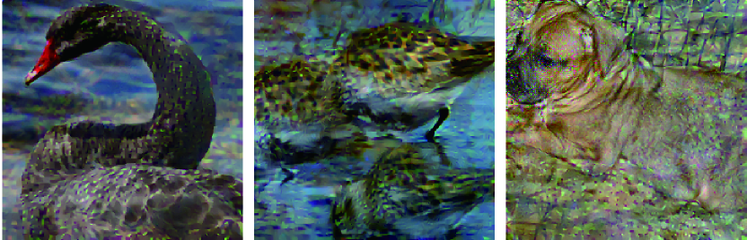
(b) RAF-GI (Ours)

Figure 3: The results of $\hat{x}$ with a batch size of 1. We reconstruct the 5000th, 7000th, and 9000th images of the ImageNet validation set in RAF-GI.

IV-D Batch Reconstruct

Reconstructed Results as Batch Size is 1

As DLG stands as a pioneering work in the GI field, laying the foundation for the development of RAF-GI, we incorporate the $\hat{x}$ of DLG into subsequent experimental comparisons, consistent with the experimental setup in GradInversion [7]. GGI [6] and RAF-GI utilize cosine similarity as the loss function. GradInversion achieves state-of-the-art GI results using the same model architecture and dataset as RAF-GI. Consequently, our comparative analysis encompasses the evaluation of visual and numerical outcomes among DLG, GGI, GradInversion [4, 6, 7], and RAF-GI. To address the mismatch between $\hat{y}$ and $x$ in large batch sizes, we sort $\hat{y}$ in ascending order, following the approach used in GradInversion.

Experiments are initially conducted with a batch size of 1 under various strategies, including RAF-GI, DLG [4], GGI [6], and GradInversion [7]. The $MI$ for each strategy is set to 10K to monitor model convergence speed, and visual representations of all $\hat{x}$ are generated and presented in Figure 2. Due to hardware limitations, the group number for all GradInversion experiments in this study is set to 3, a reduction from the original 10 specified in the reference paper [7].

To quantitatively assess performance, we employ four evaluation metrics: PSNR, SSIM, LPIPS, and MSE, and the metrics are summarized in Table III. The findings consistently demonstrate that RAF-GI outperforms other strategies in terms of reconstruction quality. When $MI$ is significantly reduced from the original settings, DLG, GGI, and GradInversion exhibit poor $\hat{x}$ performance, with the models failing to converge effectively. In contrast, RAF-GI demonstrates faster model convergence and superior $\hat{x}$ quality. We present reconstructed results for the indexes of 5000, 7000, and 9000 images in Figure 3 to illustrate the universality of the RAF-GI strategy.

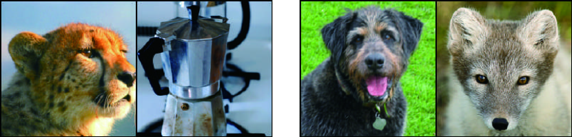
(a) Ground-truth

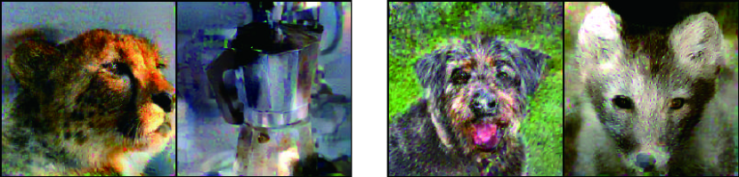
(b) RAF-GI (Ours)

Figure 4: The $\hat{x}$ result of RAF-GI when batch size is 2.

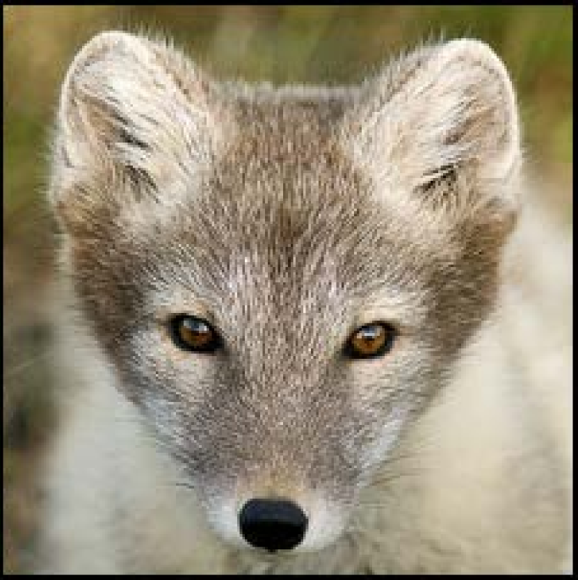
(a)

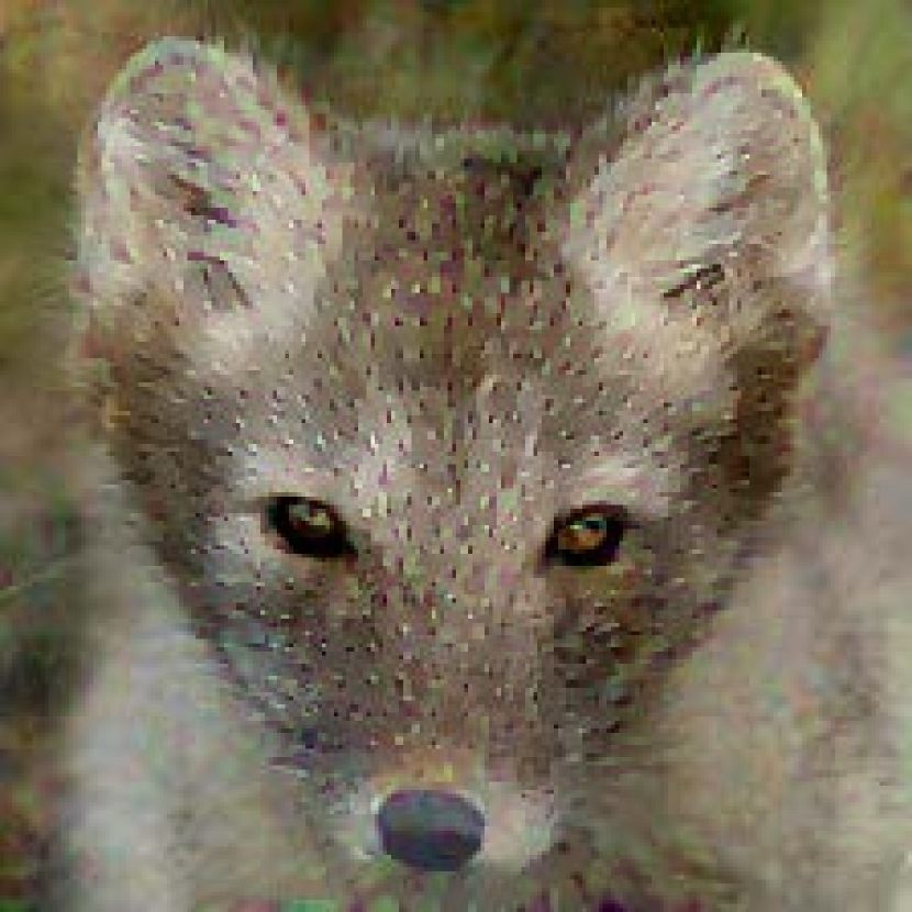
(b) 1

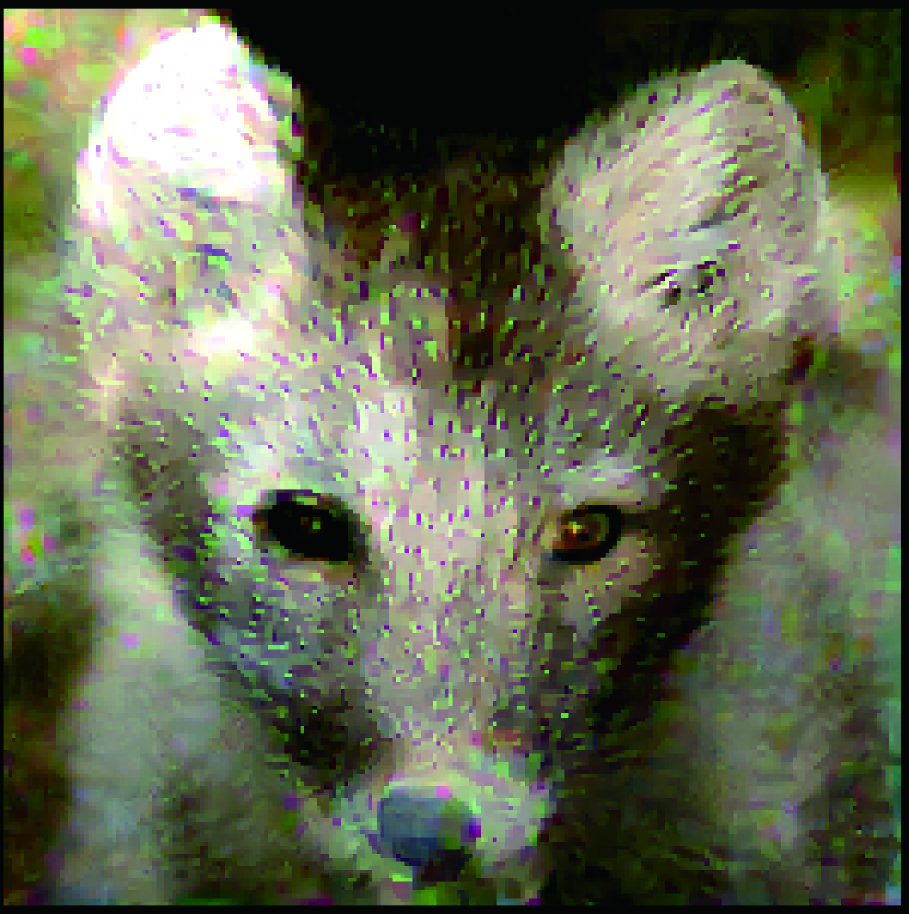
(c) 2

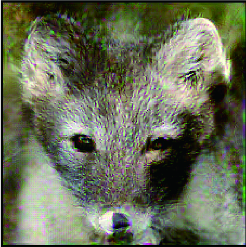
(d) 8

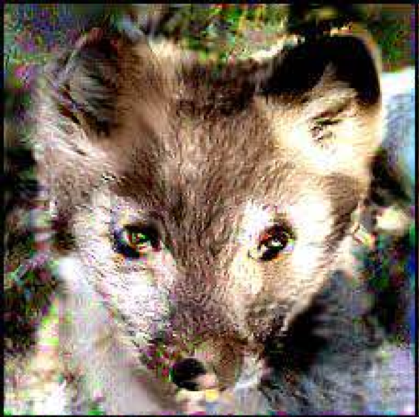
(e) 48

Figure 5: The results of GI strategies at the training batch size from 1 to 48. The first image is the ground-truth and the number under the image is the size of the training batch size.

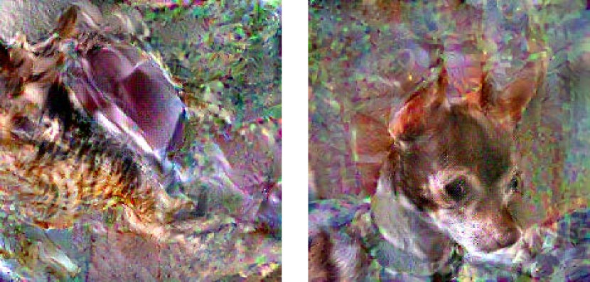
(a) RAF-GI-10K (Ours)

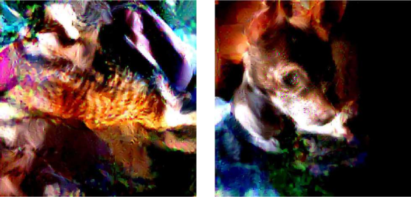
(b) GGI-192K

Figure 6: Compare RAF-GI with GGI under different restart times. Figure (a) shows the result of RAF-GI after 10K iterations, while (b) depicts the result after GGI with a total of 192K iterations.

Reconstructed Results as Batch Size $>$ 1

Figure 4 displays the $\hat{x}$ of RAF-GI with a training batch size of 2. The experimental results for a batch size of 4 are shown in the Appendix. It is important to note that $\hat{x}$ is influenced by factors such as the color and image subject of other images in the same batch. For example, the color of the third column $\hat{x}$ in Figure 4 is lighter than the corresponding $x$, but the color of the fourth column image is darker than its $x$. Next, we evaluate the attack effects of RAF-GI with a batch size increasing from 1 to 48. These results are presented in Figure 5. Observing the $\hat{x}$, RAF-GI maintains its ability to visually identify the image subject even under a large training batch size. This highlights the practicality and robustness of RAF-GI. But the color of the image in a large training batch may be shifted due to the influence of other images in the same training batch.

It is evident from these results that the quality of $\hat{x}$ decreases as the batch size increases. This underscores that increasing batch sizes can better protect user data.

Time Costs Comparison

Since GGI [6] shares the same loss function as RAF-GI and considering the unopened GradInversion source code, coupled with comprehensive considerations based on hardware limitations, we choose GGI with its original hyperparameter settings (represented as GGI-192K in Figure  8) as a comparative strategy to assess the time cost superiority of RAF-GI under a batch size of 1. GGI-192K involves 8 restarts, and the final $\hat{x}$ results are depicted in Figure 6. The results of time comparison are displayed in Figure 8. Notably, RAF-GI consistently outperforms GGI-192K in terms of reconstruction quality, even with a reduction of over 94% in the total time costs. Although DLG requires the least time, it performs poorly in terms of reconstruction quality and is not suitable for GI attacks on high-resolution images. Given that the 10K iterations of GradInversion take more than 7 hours, executing the complete GradInversion strategy, with 20K iteration times and 10 random group seeds, requires high hardware specifications for the attacker. Thus, this strategy is hard to be applied in practical training models.

Ablation Experiment

To clear the effect of each regularization terms in $\hat{x}$, we systematically incorporate each proposed regularization term into the reconstruction process. A visual and quantitative comparison of $\hat{x}$ is summarized in Figure 9 and Appendix. When no regularization term is applied, denoted as None in Figure 9, the $\hat{x}$ results exhibit significant pixel noise. The addition of $\mathbf{R}_{TV}$ enhances image quality and reduces the noise. However, $\mathbf{R}_{TV}$ introduces a noticeable shift in the $\hat{x}$ subject’s position and inaccurate colors. In the fourth column of Figure 9, we introduce $\mathbf{R}_{mean}$ to correct the color in $\hat{x}$. This operation helps increase PSNR values of $\hat{x}$. Finally, to rectify the position of the image subject, the objective function incorporates $\mathbf{R}_{canny}$. The results are in higher values of SSIM and smaller values of LPIPS in most cases, contributing to the improvement of $\hat{x}$.

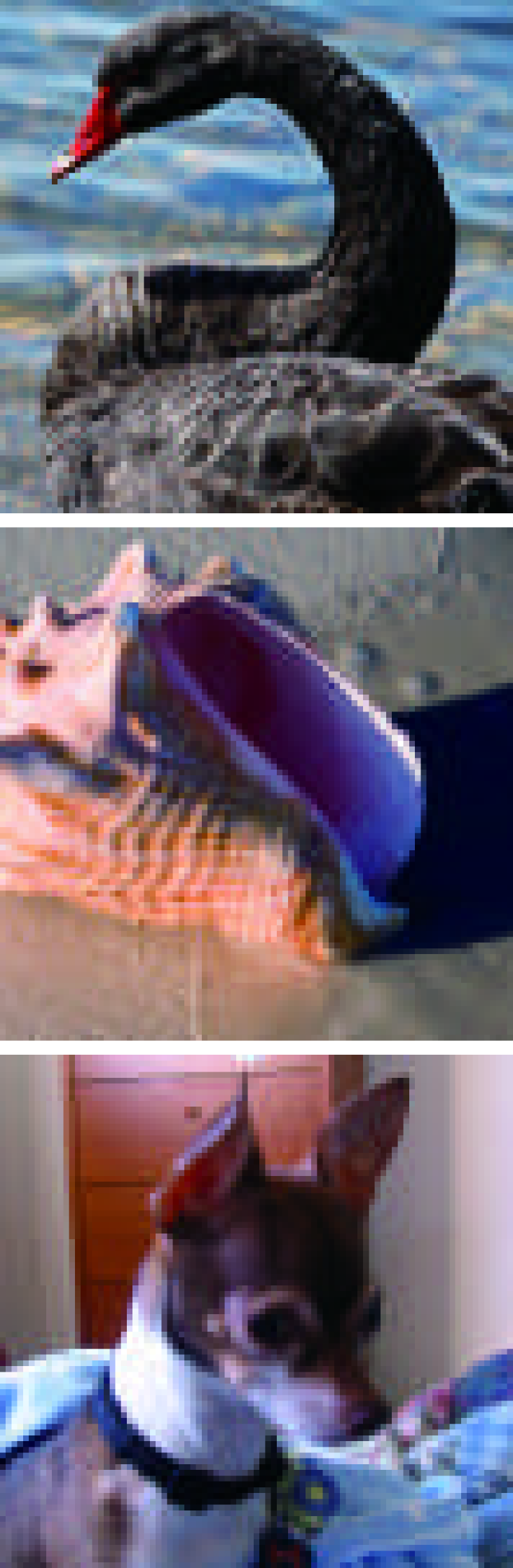
(a) Ground-truth

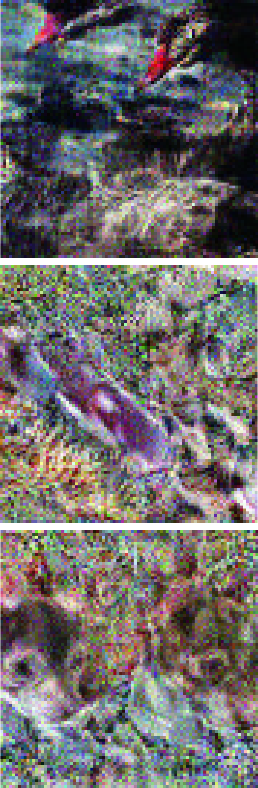
(b) None

(c) +$\mathbf{R}_{TV}$

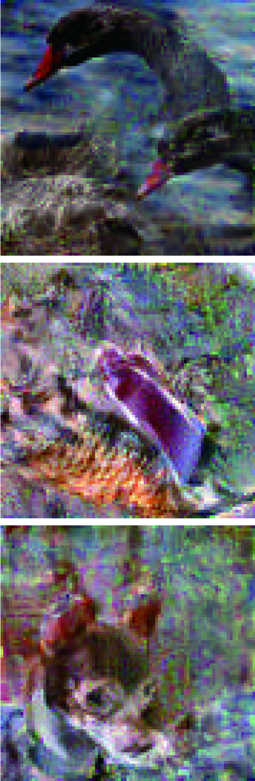
(d) +$\mathbf{R}_{mean}$

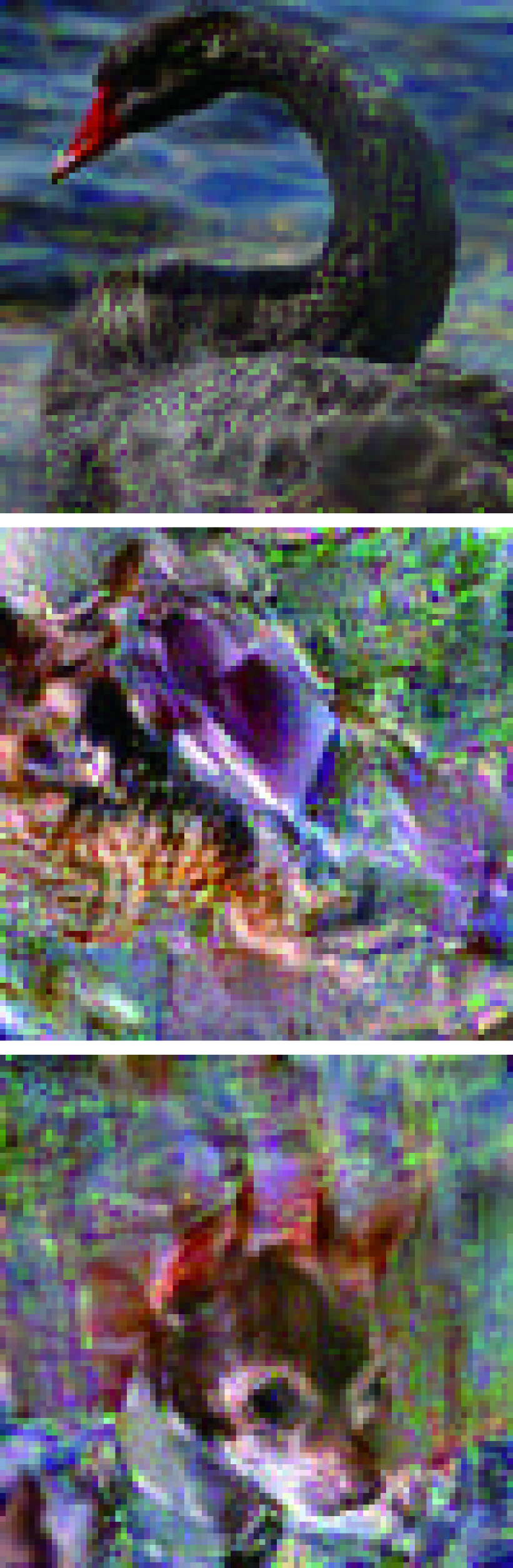
(e) +$\mathbf{R}_{ca}$

Figure 7: Ablation study of each regularization term at the batch size of 1.

Impact of $\hat{x}$ Initialization

To examine the impact of $\hat{x}$ initialization on the final $\hat{x}$, we conduct fine-tuning experiments in the Appendix. A notable finding is the superior reconstruction achieved when using gray images as the initial $\hat{x}$.

Impact of Cost Functions

Finally, we conduct fine-tuning experiments in the Appendix to examine the impact of different cost functions. Our experimental results indicate that the cosine similarity cost function significantly affects the quality of $\hat{x}$, providing a significant advantage.

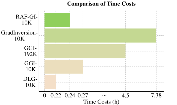
Figure 8: The comparison of time costs between different strategies at a batch size of 1 is shown in Figure 2 and Figure 6. The $\cdot K$ under the name of different strategies represents the total number of iterations for each strategy.

V Conclusion

We introduce RAF-GI, an effective gradient inversion strategy that combines two novel approaches to enhance label accuracy through ACB and improve the quality of reconstructed images in the ImageNet dataset through TEA. ACB utilizes a convolutional layer block to accurately generate labels for a single batch of images. The experimental results highlight the efficiency of TEA in significantly reducing time costs compared to prior methods, consistently achieving superior reconstructed image results. These findings emphasize the practicality of gradient inversion in real-world applications, underscoring the importance of safeguarding gradients.

In the future, our work will explore additional applications and optimizations of RAF-GI to enhance its performance across diverse scenarios. Furthermore, our research scope will extend into the domain of natural language reconstruction within Transformer models, addressing more complex text reconstruction tasks.

1 Input: $G_{1}$: the column-wise summation of the last FC layer gradients; $\textbf{ACB}(\cdot)$: propagation in the additional convolutional layer; $K$: the training batch size.

2 Parameter: $G_{2}$: the result of the linear transformation of $G_{1}$; $|\cdot|$: the number of elements in a vector or matrix; $N$: the total number of classes; $argsort(\cdot)$: sort $\cdot$ in decreasing order and obtain the index of $\cdot$; $sum(\cdot)[-1]$: summation along the column-wise; $in(\cdot)$: check if an element exists in the vector; $L_{k}$:the reconstructed labels $\hat{y}$ from $G_{1}$ with $|L_{k}|$ as $k$; $L_{ACB}$: the $\hat{y}$ from ACB; $pro_{ACB}$: the probability of labels after ACB; $pro^{\prime}_{ACB}$:the result of the linear transformation of $pro{ACB}$; $cat(\cdot)$: concatenate two vectors into one vector.

3 Output: $L$: the reconstructed labels $\hat{y}$.

1:  $G_{2}=G_{1}\times 10^{17}$

2:  $|L_{k}|=0$

3:  $|L_{ACB}|=0$

4:  for i = 0, …, N-1 do

5:     if $G_{1}[i]<0$ then

6:        $L_{k}\leftarrow arg~{}sort(G_{1}[i])$

7:     end if

8:  end for

9:  $|L_{k}|=k$

10:  $pro_{ACB}=sum(ACB(G_{2}))[-1]$

11:  $pro^{\prime}_{ACB}=pro_{ACB}/10^{10}$

12:  $id_{mid}=arg_{s}ort(pro^{\prime}_{ACB})$

13:  if $k<K$ then

14:     for i = 0, …, N-1 do

415:        if $id_{mid}[i]~{}in~{}L_{k}~{}and$

$(pro^{\prime}_{ACB}[id_{mid}[i]]-pro^{\prime}_{ACB}[id_{mid}[i+1]])>0.4$ then

16:           $L_{ACB}\leftarrow id_{mid}[i]$.

17:        end if

18:     end for

19:  end if

20:  $m=0$

21:  if $|L_{ACB}|<K-k$ then

22:     $L_{ACB}\leftarrow L_{k}[m]$

23:     $m=m+1$

24:  end if

25:  return $L\leftarrow cat(L_{k},L_{ACB})$

Algorithm 1 Label Restoration in ACB

VI The Label Restoration in ACB

In this section, we present the thresholds chosen for ACB based on numerous experiments in the first subsection. Following that, the second subsection provides the pseudocode illustrating the working process of ACB.

VI-A The Threshold Parameter comparison in ACB

In Table IV, we compare ACB label accuracy on the ImageNet dataset’s validation set under various thresholds. A threshold of 0.4 exhibits superior performance across different batch sizes in terms of label recovery accuracy. Consequently, we adopted 0.4 as the selected threshold in the final scheme design.

	0.3	0.4	0.5
1	100%	100%	100%
2	98.90%	98.90%	98.75%
4	91.78%	91.95%	90.98%
8	87.25%	87.01%	86.69%
16	83.57%	83.95%	83.83%
32	81.18%	80.96%	81.07%
64	79.23%	79.24%	79.29%

TABLE IV: Comparison of label reconstruction using ACB under different threshold hyperparameters on the ImageNet dataset’s validation set. We evaluate the average label recovery accuracy across 1K random samples with various batch sizes. Optimal values are highlighted in bold.

1 Input: $G_{1}$: the column-wise summation of the last FC layer gradients; $CA(\hat{x}_{i},thre_{1},thre_{2})$: Canny edge detection of image $\hat{x}$ with two thresholds $thre_{1}$ and $thre_{2}$.

2 Parameter: $mean(\cdot)$: the mean value of $\cdot$; $max(\cdot)$: the maximum value of $\cdot$; $fin$: the threshold to obtain edges from $G_{1}$; $ca_{fin-reg}$: the pixel site set where the gradient value is larger than $fin$; $|\cdot|$: the number of elements in a vector or matrix; $img_{row},img_{col}$: the ground-truth image matrix dimensions; $index(\cdot)$: the index of $\cdot$; $gra_{row},gra_{col}$: the element number of $ca_{reg}$, and $gra_{row}$ is equal to $gra_{col}$.

3 Output: ${R}_{canny}$: the value of $\mathbf{R}_{canny}$.

4

1:  $fin=(max(G_{1})-mean(G_{1}))\times 0.6$

2:  for $i~{}from~{}0~{}to~{}|G_{1}|$ do

3:     if $G_{1}[i]>fin$ then

4:        $ca_{fin}\leftarrow G_{1}[i]$

5:     end if

56:  end for

7:  $gra_{row}=|ca_{fin}|$

8:  $gra_{col}=|ca_{fin}|$

9:  for $j~{}from~{}0~{}to~{}gra_{row}$ do

10:     $ca_{fin-reg}\leftarrow[\lfloor ca_{fin}[j]\times img_{row}/gra_{row}\rfloor,\lfloor ca_{fin}[j]\times img_{col}/gra_{col}\rfloor]$

11:  end for

612:  $ca_{reg}\leftarrow ca_{fin-reg}[1/2\times gra_{row}]$

13:  $ca_{t}\leftarrow CA(\hat{x},0.8,0.9)$

14:  $\hat{c}a_{reg}\leftarrow ca_{t}[1/2\times|ca_{t}|]$

715:  ${R}_{canny}\leftarrow\lVert ca_{reg}-\hat{ca_{reg}}\rVert_{2}$

16:  return ${R}_{canny}$

Algorithm 2 Canny edge detection regularization term $\mathbf{R}_{canny}$

1 Input: $\nabla W$: the ground-truth gradients; $\nabla W^{\prime}$: the reconstructed image gradients; $\hat{y}$: the reconstructed labels; $MI$: the maximum iteration times; $\mathbf{R}_{TV}$: the total variance regularization term; $\mathbf{R}_{mean}$: the three-channel mean regularization term; $\mathbf{R}_{canny}$: the Canny edge detection regularization term; $\alpha_{TV}$: the scaling factor for $\mathbf{R}_{TV}$; $\alpha_{mean}$: the scaling factor for $\mathbf{R}_{mean}$; $\alpha_{ca}$: the scaling factor for $\mathbf{R}_{canny}$.

2 Parameter: $gray$: gray image; $cos(\cdot)$: the cosine similarity function; $\mathbf{R}_{reg}$: the value of three regularization terms; $argmin(\cdot)$: get the minimum value of $\cdot$; $M_{back}(\cdot,\cdot)$: the backpropagation of the model.

3 Output: $\hat{x}$: the reconstructed image.

1:  $\hat{x}=gray$

2:  for $i~{}from~{}0~{}to~{}MI-1$ do

3:     $\mathbf{R}_{reg}=\alpha_{TV}\mathbf{R}_{TV}+\alpha_{mean}\mathbf{R}_{mean}+\alpha_{ca}\mathbf{R}_{canny}$

4:     $\hat{x}=\mathop{argmin}\limits_{\hat{x},\hat{y}}1-cos(\nabla W^{\prime},\nabla W)+\mathbf{R}_{reg}$

5:     $M_{back}(\hat{x},\hat{y})$

6:     update $\hat{x}$

7:  end for

8:  return $\hat{x}$

Algorithm 3 TEA

Regularization	Metrics
Terms	PSNR $\uparrow$	SSIM $\uparrow$	LPIPS $\downarrow$	MSE $\downarrow$
None	13.30	0.0079	0.6146	0.3033
	14.51	0.0092	0.7576	0.2296
	14.94	0.0091	0.7039	0.2042
$+\mathbf{R}_{TV}$	14.89	0.0768	0.5073	0.0954
	16.08	0.0591	0.6068	0.0995
	16.32	0.0820	0.5899	0.0737
$+\mathbf{R}_{mean}$	13.81	0.1254	0.4202	0.0587
	16.30	0.0514	0.5640	0.0822
	16.07	0.1065	0.6116	0.0810
$+\mathbf{R}_{ca}$	16.27	0.2979	0.1998	0.0356
	17.47	0.0572	0.4909	0.0959
	15.87	0.1183	0.5762	0.0812

TABLE V: The metric values in the results of ablation experiments are depicted in Figure 9. Optimal values, highlighted in bold font, are predominantly associated with RAF-GI, which corresponds to the last row in the table.

$\hat{x}$	Metrics
	PSNR $\uparrow$	SSIM $\uparrow$	LPIPS $\downarrow$	MSE $\downarrow$
RAF-GI	17.47	0.0572	0.4909	0.0959
	15.87	0.1183	0.5762	0.0812
RAF-GI-ran	12.54	0.0171	0.6656	0.2824
	10.33	0.0393	0.5922	0.2438
DLG	3.55	0.0156	1.4242	2.8638
	3.56	0.0143	1.4843	2.8553
DLG-gray	11.47	0.0089	1.4718	1.1243
	11.59	0.0076	1.4087	1.0453
GGI	12.18	0.0137	0.6928	0.3568
	11.60	0.0378	0.6813	0.3906
GGI-gray	15.56	0.0557	0.6032	0.0935
	17.15	0.1201	0.5952	0.0854

TABLE VI: The metric values for different gradient inversion strategies, based on random and gray image initializations of $x$, are presented in Figure 10. Notably, optimal values, highlighted in bold font, are consistently associated with gray image initializations of $x$.

VI-B The Pseudocode of Label Restoration

To elimate the previous works assumation that no-repeat labels in one training batch, the most difficult to solve is that obataining the repeated labels in one training batch. ACB solves this problem with 20% label accuracy improment. We present pseudocode in Algorithm 1 for label restoration. Lines 4-8 extract $L_{k}$, while lines 10-19 manage the $L_{ACB}$ procedure. Ultimately, concatenation of $L_{k}$ and $L_{ACB}$ ensures the restoration of labels aligns with the batch size $K$.

$\hat{x}$	Metrics
	PSNR $\uparrow$	SSIM $\uparrow$	LPIPS $\downarrow$	MSE $\downarrow$
RAF-GI	17.47	0.0572	0.4909	0.0959
	15.87	0.1183	0.5762	0.0812
RAF-GI-$\ell_{2}$	14.00	0.0089	1.1852	0.1949
	14.29	0.0081	0.9543	0.2015
DLG	3.55	0.0156	1.4242	2.8638
	3.56	0.0143	1.4843	2.8553
DLG-cos	8.06	0.0096	0.9278	1.0139
	8.53	0.0092	0.9091	0.9108
GGI	12.18	0.0137	0.6928	0.3568
	11.60	0.0378	0.6813	0.3906
GGI-$\ell_{2}$	7.61	0.0094	1.4718	1.1243
	7.93	0.0095	1.4087	1.0453

TABLE VII: The metric values for different gradient inversion strategies, based on cosine similarity and $\ell_{2}$ cost functions, are shown in Figure 11. The optimal values, indicated in bold font, are all associated with RAF-GI.

VII The Image Reconstructed in TEA

In this section, we present the detailed pseudocode of $\mathbf{R}_{canny}$, illustrating the workflow of the Canny edge detection regularization term in the first subsection. The pseudocode for TEA depicts the workflow of the TEA strategy throughout the entire maximum iteration times in the second subsection.

VII-A Pseudocode of $\mathbf{R}_{canny}$

The pseudocode for calculating the regularization term $\mathbf{R}_{canny}$ is presented in Algorithm 2. Lines 1-6 depict the process of obtaining edges from the ground-truth gradient, lines 9-11 represent the workflow for the base-point of $x$, while lines 12-14 handle the $\hat{x}$ edge obtaining, and line 15 is the $\ell_{2}$ distance calculation process. The result of $\mathbf{R}_{canny}$ is used to penalize the large gap between $x$ and $\hat{x}$.

VII-B Pseudocode of TEA

We present pseudocode in Algorithm 3 for the execution of TEA. Lines 2-6 encompass the entire iteration process of TEA. Finally, TEA returns $\hat{x}$ corresponding to the minimum loss function value as the final result.

VIII Experiments

In this section, we provide detailed experiment settings in the first subsection. Following that, the second subsection presents visual results and metric values from the ablation experiment. Finally, we investigate the effects of $x$ initialization and cost functions on the final $\hat{x}$ under a batch size of 1 in the third and fourth subsections, respectively.

VIII-A Experiments Details

We utilize the pre-trained ResNet-50 as the adversarial attack model, implementing the RAF-GI strategy to invert images of size 224$\times$224 pixels from the validation set of the 1000-class ImageNet ILSVRC 2021 dataset [15]. In the RAF-GI experiment, we carefully configured hyperparameters, setting $\alpha_{TV}=1e-1$, $\alpha_{mean}=1e-3$, $\alpha_{ca}=1e-2$, and the learning rate $lr=1e-2$ during the maximum iterations $MI=10K$ at the batch size of 1. The $lr$ decreases after 2/7 of the iterations and is reduced by a factor of 0.2 in all experiments. RAF-GI is to restart only once, while GGI [6] requires eight restarts. The inversion process of RAF-GI is accelerated using one NVIDIA A100 GPU, coupled with the Adam optimizer.

VIII-B The Ablation Experiment

We present the visual ablation experiment results in Figure 9 and metrics for quantitative comparisons in Table V. The optimal choice for reconstructing ground-truth images is observed in the final row (RAF-GI) in most cases. Without any regularization term (denoted as ”None” in the second column of Figure 9), the $\hat{x}$ exhibits poor performance with multiple subjects in the image and numerous noises. The introduction of $\textbf{R}_{TV}$ into the reconstruction strategy results in a significant reduction in noise and increased PSNR values. Addition of $\textbf{R}_{mean}$ to the reconstruction strategy eliminates multi-subjects and color distortions in $\hat{x}$, leading to higher SSIM values. Lastly, incorporating $\textbf{R}_{canny}$ corrects the image subject site, resulting in reduced values of LPIPS and MSE.

(a) Ground-truth

(b) None

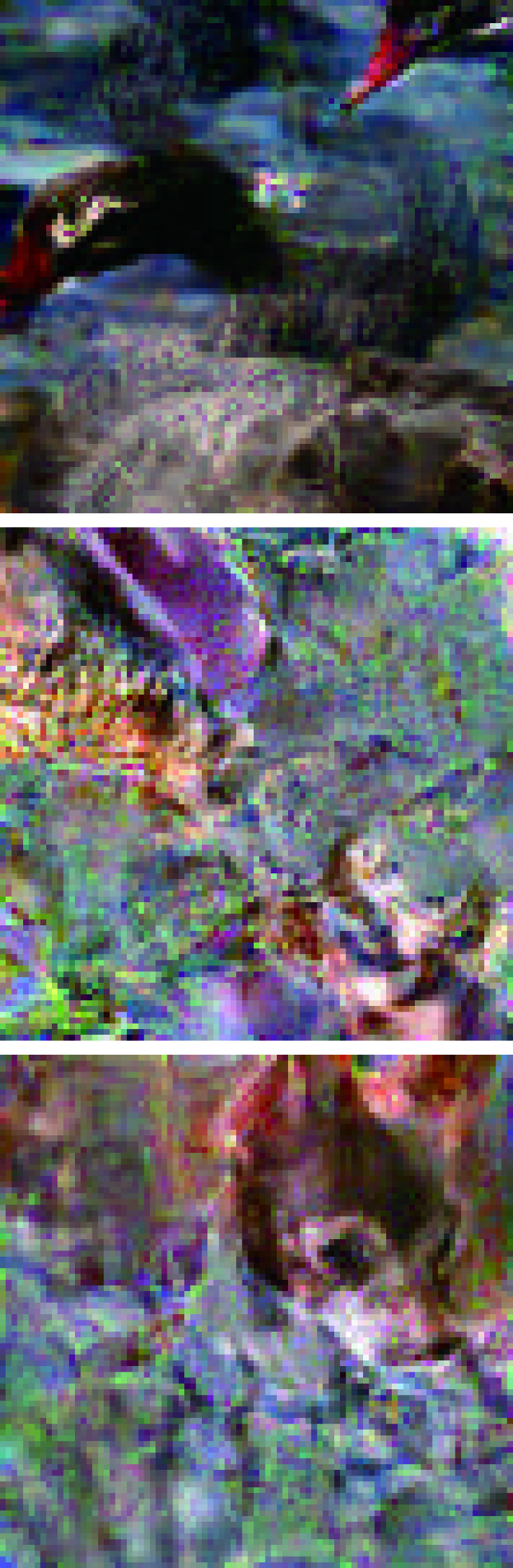
(c) +$\mathbf{R}_{TV}$

(d) +$\mathbf{R}_{mean}$

(e) +$\mathbf{R}_{ca}$

Figure 9: Ablation study of each regularization term with a batch size of 1. The results reveal that the optimal $\hat{x}$ consistently corresponds to the last column (RAF-GI).

(a) Ground-truth

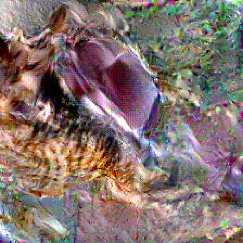
(b) RAF-GI

(c) RAF-GI-ran

(d) DLG-gray

(e) DLG

(f) GGI-gray

(g) GGI

(h) Ground-truth

(i) RAF-GI

(j) RAF-GI-ran

(k) DLG-gray

(l) DLG

(m) GGI-gray

(n) GGI

Figure 10: Different gradient inversion strategies based on random and gray image initializations of $x$.

(a) Ground-truth

(b) RAF-GI

(c) RAF-GI-$\ell_{2}$

(d) DLG

(e) DLG-cos

(f) GGI

(g) GGI-$\ell_{2}$

(h) Ground-truth

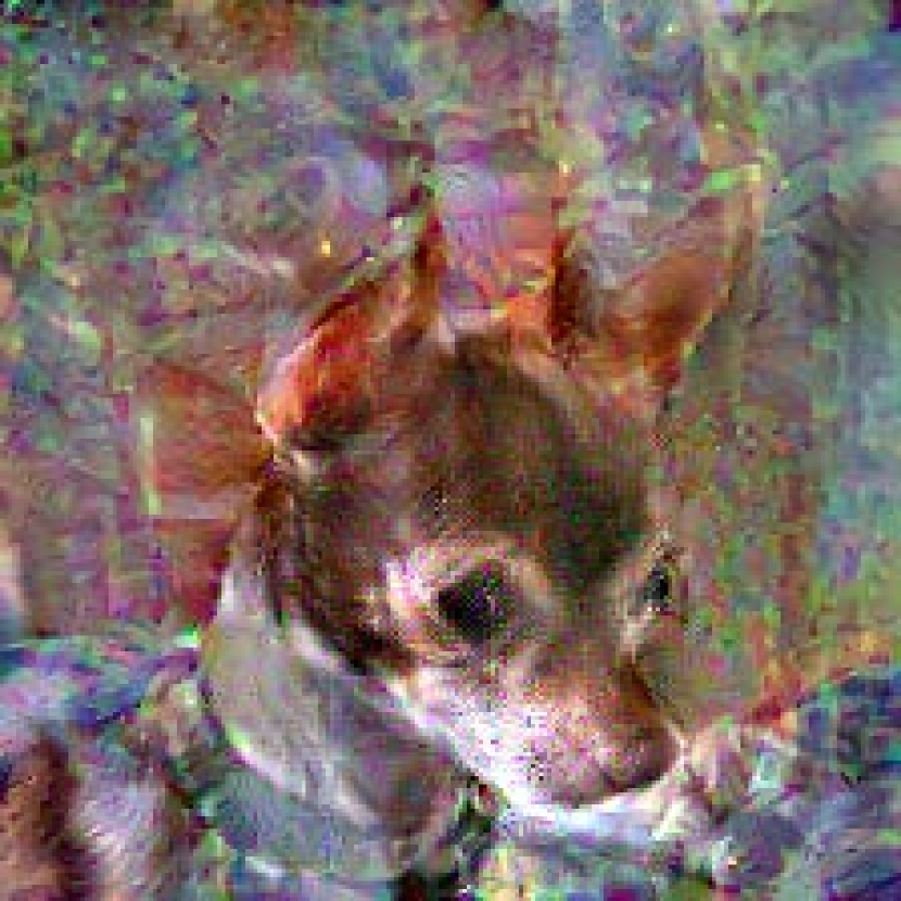
(i) RAF-GI

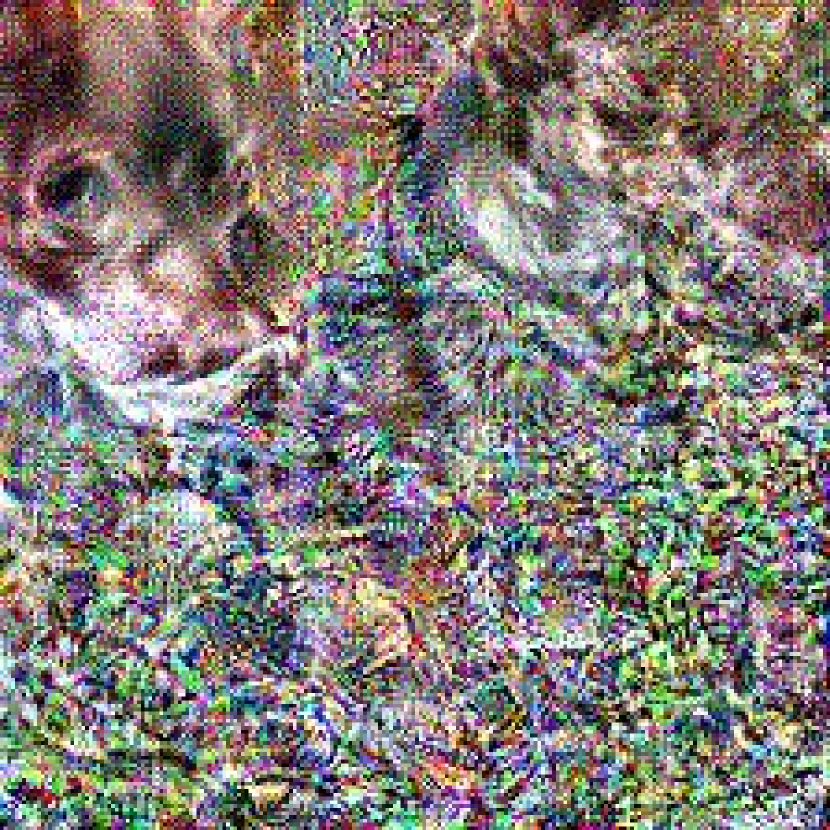
(j) RAF-GI-$\ell_{2}$

(k) DLG

(l) DLG-COS

(m) GGI

(n) GGI-$\ell_{2}$

Figure 11: Different gradient inversion strategies based on cosine similarity and $\ell_{2}$ cost functions.

VIII-C Impact of $\hat{x}$ Initialization

To assess the impact of $\hat{x}$ initialization on the final result, RAF-GI employs a random image as the initial $\hat{x}$ (RAF-GI-ran), while DLG [4] and GGI [6] use gray images as the initial $\hat{x}$ (DLG-gray, GGI-gray). Visual results and evaluation metrics for the final $\hat{x}$ are presented in Figure 10 and Table VI. Notably, comparisons between DLG and DLG-gray, GGI and GGI-gray, and RAF-GI-ran and RAF-GI highlight the superior reconstruction achieved when using gray images as the initial $\hat{x}$ (DLG-gray, GGI-gray, and RAF-GI). This underscores the critical role of the initial $\hat{x}$ in enhancing the quality of the final reconstruction. While GGI-gray shows better results in terms of PSNR and SSIM values in the second reconstructed image, it is important to note that the image subject position and visual effects may be compromised, revealing the limitations of relying solely on a single evaluation metric.

VIII-D Impact of Cost Functions

DLG [4] and GGI [6] employ distinct cost functions to quantify the difference between $\nabla W^{\prime}$ and $\nabla W$. Since GradInversion [7] has already investigated the impact of the cost function on the quality of $\hat{x}$, we won’t experiment with the GradInversion transformation cost function in this study. We utilize various cost functions for DLG, GGI, and RAF-GI. Specifically, we consider DLG-$\cos$, GGI-$\ell_{2}$, and RAF-GI-$\ell_{2}$, modifying the cost function to cosine similarity and $\ell_{2}$ distance. Visual results of reconstructed images and corresponding metrics are provided in Figure 11 and Table VII. Notably, cosine similarity exhibits a stronger tendency to generate high-quality $\hat{x}$. All strategies based on the cosine similarity cost function have higher values in PSNR and smaller LPIPS values than those with the $\ell_{2}$ distance cost function. This observation deviates from the findings in GradInversion [7]. The discrepancy may be attributed to different regularization terms. In our experiments, the choice of the cost function significantly impacts the quality of $\hat{x}$, with cosine similarity showing a substantial advantage.

References

- [1] J. Konečnỳ, H. B. McMahan, F. X. Yu, P. Richtárik, A. T. Suresh, and D. Bacon, “Federated learning: Strategies for improving communication efficiency,” arXiv preprint arXiv:1610.05492, 2016.
- [2] T. Li, M. Sanjabi, A. Beirami, and V. Smith, “Fair resource allocation in federated learning,” arXiv preprint arXiv:1905.10497, 2019.
- [3] J. Chen, X. Pan, R. Monga, S. Bengio, and R. Jozefowicz, “Revisiting distributed synchronous sgd,” arXiv preprint arXiv:1604.00981, 2016.
- [4] L. Zhu, Z. Liu, and S. Han, “Deep leakage from gradients,” Advances in neural information processing systems, vol. 32, 2019.
- [5] B. Zhao, K. R. Mopuri, and H. Bilen, “idlg: Improved deep leakage from gradients,” arXiv preprint arXiv:2001.02610, 2020.
- [6] J. Geiping, H. Bauermeister, H. Dröge, and M. Moeller, “Inverting gradients-how easy is it to break privacy in federated learning?” Advances in Neural Information Processing Systems, vol. 33, pp. 16 937–16 947, 2020.
- [7] H. Yin, A. Mallya, A. Vahdat, J. M. Alvarez, J. Kautz, and P. Molchanov, “See through gradients: Image batch recovery via gradinversion,” in Proceedings of the IEEE/CVF Conference on Computer Vision and Pattern Recognition, 2021, pp. 16 337–16 346.
- [8] J. Zhu and M. Blaschko, “R-gap: Recursive gradient attack on privacy,” arXiv preprint arXiv:2010.07733, 2020.
- [9] Q. Yang, Y. Liu, T. Chen, and Y. Tong, “Federated machine learning: Concept and applications,” ACM Transactions on Intelligent Systems and Technology (TIST), vol. 10, no. 2, pp. 1–19, 2019.
- [10] W. Wei, L. Liu, M. Loper, K.-H. Chow, M. E. Gursoy, S. Truex, and Y. Wu, “A framework for evaluating gradient leakage attacks in federated learning,” arXiv preprint arXiv:2004.10397, 2020.
- [11] A. Hatamizadeh, H. Yin, P. Molchanov, A. Myronenko, W. Li, P. Dogra, A. Feng, M. G. Flores, J. Kautz, D. Xu et al., “Do gradient inversion attacks make federated learning unsafe?” IEEE Transactions on Medical Imaging, 2023.
- [12] C. Chen and N. D. Campbell, “Understanding training-data leakage from gradients in neural networks for image classification,” arXiv preprint arXiv:2111.10178, 2021.
- [13] X. Jin, P.-Y. Chen, C.-Y. Hsu, C.-M. Yu, and T. Chen, “Cafe: Catastrophic data leakage in vertical federated learning,” Advances in Neural Information Processing Systems, vol. 34, pp. 994–1006, 2021.
- [14] J. Canny, “A computational approach to edge detection,” IEEE Transactions on Pattern Analysis and Machine Intelligence, vol. PAMI-8, no. 6, pp. 679–698, 1986.
- [15] J. Deng, W. Dong, R. Socher, L.-J. Li, K. Li, and L. Fei-Fei, “Imagenet: A large-scale hierarchical image database,” in 2009 IEEE conference on computer vision and pattern recognition. Ieee, 2009, pp. 248–255.
- [16] L. Deng, “The mnist database of handwritten digit images for machine learning research [best of the web],” IEEE signal processing magazine, vol. 29, no. 6, pp. 141–142, 2012.
- [17] H. Xiao, K. Rasul, and R. Vollgraf, “Fashion-mnist: a novel image dataset for benchmarking machine learning algorithms,” arXiv preprint arXiv:1708.07747, 2017.
- [18] B. Recht, R. Roelofs, L. Schmidt, and V. Shankar, “Do cifar-10 classifiers generalize to cifar-10?” arXiv preprint arXiv:1806.00451, 2018.
- [19] J. Xu, C. Hong, J. Huang, L. Y. Chen, and J. Decouchant, “Agic: Approximate gradient inversion attack on federated learning,” in 2022 41st International Symposium on Reliable Distributed Systems (SRDS). IEEE, 2022, pp. 12–22.
- [20] X. Dong, H. Yin, J. M. Alvarez, J. Kautz, and P. Molchanov, “Deep neural networks are surprisingly reversible: a baseline for zero-shot inversion,” arXiv e-prints, pp. arXiv–2107, 2021.
- [21] T. Hideaki, “AIJack,” Jun. 2023. [Online]. Available: https://github.com/Koukyosyumei/AIJack