Mean-Field Microcanonical Gradient Descent

Abstract

Microcanonical gradient descent is a sampling procedure for energy-based models allowing for efficient sampling of distributions in high dimension. It works by transporting samples from a high-entropy distribution, such as Gaussian white noise, to a low-energy region using gradient descent. We put this model in the framework of normalizing flows, showing how it can often overfit by losing an unnecessary amount of entropy in the descent. As a remedy, we propose a mean-field microcanonical gradient descent that samples several weakly coupled data points simultaneously, allowing for better control of the entropy loss while paying little in terms of likelihood fit. We study these models in the context of financial time series, illustrating the improvements on both synthetic and real data.

1 Introduction

The defining characteristic of a well-behaved generative model is the balance between its ability to, on the one hand produce samples that are typical of the training data, while on the other hand having a significant amount of diversity within its samples. For example, a generative adversarial network (GAN) which has suffered mode collapse could produce great samples within one mode but would then only produce samples within that one mode. On one extreme, we therefore have a model which exactly reproduces the empirical distribution of the training set, while on the other extreme, we have a model which produces samples of Gaussian white noise regardless of the training data. Formally, we can view this in terms of the reverse Kullback–Leibler (KL) divergence (Papamakarios et al., 2021) of the generative model $q$ with respect to the true distribution $p$:

$$\mathcal{D}_{\text{KL}}(q\parallel p)=-H(q)-\mathbb{E}_{q}[\log p(X)],$$

where $H(q)$ denotes the differential entropy of $q$ and $\mathbb{E}_{q}$ is the expected value with respect to $q$. To achieve a good fit, that is, a low KL divergence, we thus want to simultaneously maximize the entropy $H(q)$ and the log-likelihood $\mathbb{E}_{q}[\log p(X)]$ of $p$ under the approximation $q$.

One popular family of generative models is that of the energy-based model (Geman & Geman, 1984), also known as a canonical or macrocanonical model (Jaynes, 1957), which takes an energy vector $\Phi:\mathcal{X}\to\mathbb{R}^{K}$ defined on the sample space $\mathcal{X}$ and produces samples from the distribution that maximizes the entropy given the constraint $\mathbb{E}_{q}[\Phi(X)]=\alpha$, fixing the expected energy vector to some point $\alpha\in\mathbb{R}^{K}$. A macrocanonical model can in many cases be approximated by a microcanonical model, which similarly maximizes entropy, but over the set

$$\Omega_{\varepsilon}=\{x\in\mathcal{X}:\|\Phi(x)-\alpha\|\leq\varepsilon\},$$ (1)

for some $\varepsilon>0$ (Lanford, 1975; Ellis et al., 2000; Touchette, 2015). This $\Omega_{\varepsilon}$ is known as the microcanonical set of width $\varepsilon$. Without loss of generality, we shall assume that $\alpha=0$ (otherwise, we simply redefine $\Phi(x)$ to be $\Phi(x)-\alpha$). This microcanonical approximation is often useful when it is reasonable to assume that the energy vector concentrates in a region of high probability. For example, in the context of stationary time series of sufficiently long duration $d$, this amounts to working with energy vectors defined as the time average of time-shift equivariant potentials.

While conceptually simple and theoretically useful, both macrocanonical and microcanonical models suffer from difficulties in sampling for high-dimensional sample spaces. To mitigate this, the microcanonical gradient descent model (MGDM) was introduced by Bruna & Mallat (2019) as an approximation of the microcanonical model which is easier to sample from. MGDM is defined as the pushforward of Gaussian white noise by way of a sequence of gradient descent steps that seek to minimize the objective

$$L(x)=\frac{1}{2}\|\Phi(x)\|^{2}.$$ (2)

Thus samples from the MGDM are generated by sampling $x_{0}$ from $\mathcal{N}(0,\sigma^{2}\text{I}_{d})$ for some initial variance $\sigma^{2}$ and updating the sample using

$$x_{t+1}=g(x_{t})\coloneqq x_{t}-\gamma J_{\Phi}^{\top}(x_{t})\Phi(x_{t}),$$ (3)

where $\gamma$ is the step size and $J_{\Phi}$ is the Jacobian of $\Phi$. This is typically iterated for a fixed number of steps $T$ or until $x_{t}$ reaches the microcanonical set $\Omega_{\varepsilon}$ (Leonarduzzi et al., 2019; Morel et al., 2023).

While having been successfully applied in a variety of domains (Bruna & Mallat, 2019; Leonarduzzi et al., 2019; Zhang & Mallat, 2021; Brochard et al., 2022; Cheng et al., 2023; Auclair et al., 2023; Morel et al., 2023), the MGDM suffers from a problem of entropy collapse. Indeed, each gradient step in (3) has the effect of reducing the entropy of the initial distribution, resulting in a final distribution which may yield a good log-likelihood (i.e., that will produce samples with characteristics similar to the training data), but which do not contain enough variability to constitute an accurate generative model. To remedy this, we propose a variant of the MGDM, called the mean-field microcanonical gradient descent model (MF-MGDM), which generates a batch of samples such that their mean energy vector satisfies the necessary constraints. In this model, the initial distribution is not so much contracted as transported through the energy space to the required point while maintaining much of its initial entropy. Experiments for known distributions show a significant reduction in KL divergence and results on experimental data indicate a better qualitative fit compared to samples from the conventional MGDM.

The structure of this article is as follows. Section 2 surveys the literature on energy-based models and the MGDM in particular while Section 3 illustrates the entropy collapse observed in the MGDM. A proposed solution to this is introduced in Section 4 in the form of the MF-MGDM and numerical results supporting this algorithm are presented in Section 5. Python code to reproduce the results in this paper may be found at https://github.com/MarcusHaggbom/mf-mgdm.

2 Related Work

In energy-based methods, the goal is to find an energy function $E:\mathcal{X}\to\mathbb{R}$ such that the Gibbs density $q(x)\propto\exp(-E(x))$ approximates the true distribution well. This is the macrocanonical maximum entropy distribution (Cover & Thomas, 2006). Sampling from this distribution is typically done with MCMC methods, and is challenging but has been implemented in high dimensions, e.g. with Langevin dynamics (Du & Mordatch, 2019):

$$x_{t+1}=x_{t}-\frac{1}{2}\gamma\nabla E(x_{t})+\sqrt{\gamma}\varepsilon_{t},$$

which bears a resemblance with a noisy version of the MGDM when $E$ is the gradient descent loss $L$ in (2).

The microcanonical gradient descent model was introduced in (Bruna & Mallat, 2019). It has been used in a variety of applications, such as cosmology (Cheng et al., 2023; Auclair et al., 2023) and texture synthesis (Brochard et al., 2022; Zhang & Mallat, 2021). In these contexts, the model is often paired with various extensions of the scattering transform (Mallat, 2012) used as features in the energy function. The scattering transform is a composition of wavelet transforms and non-linearities, and can be seen as a convolutional neural net with predefined weights (Mallat, 2016). Apart from its use as an energy function in generative models, it has also found applications in image classification (Bruna & Mallat, 2013; Oyallon et al., 2019), audio similarity measurement (Andén et al., 2019; Lostanlen et al., 2021), molecular energy regression (Eickenberg et al., 2017), and heart beat classification (Warrick et al., 2020) among others.

In the context of finance, the MGDM has been used to generate sample paths of time series, with focus on the design of the energy function such that the approximations capture some of the typical structures that financial time series typically exhibit. In (Leonarduzzi et al., 2019), it is shown that the time-average of the second-order scattering transform encodes heavy tails, and that including also phase harmonic correlations (Mallat et al., 2019) encapsulates temporal asymmetries. An extension of this representation is known as the scattering spectrum (Morel et al., 2023), which provides a more sparse feature representation and is shown to capture multiscale properties of rough paths such as fractional Brownian motion.

Another popular feature representation for rough paths is the truncated signature (Lyons, 2014). The full signature of a path is a lossless representation up to time parametrization, and the truncation error decreases as the inverse of the factorial. In financial time series generation, this encoding has proved efficient for other generative models that involve training, such as variational autoencoders (Buehler et al., 2020) and Wasserstein GANs (Ni et al., 2021).

3 Overfitting to Target Energy

As stated, the MGDM works by pushing samples from the initial distribution towards some target energy vector which is our best approximation of the mean energy under the true distribution. It is evident that if we for some reason suspect we have a poor estimate of the mean energy, then we do not want to push our samples too close to the target, as we will then risk overfitting to the bias. What is also the case, however, is that the same principle holds even if we know the exact mean energy, as we will always lose entropy through the gradient descent process. It is therefore important to not overfit to the target energy, no matter how good the estimate is.

3.1 An Illustrative Example

As an example, take the AR(1) model with parameter $\varphi$ and conditional variance $\sigma^{2}$

$$x_{i}=\varphi x_{i-1}+\sigma\varepsilon_{i},$$ (4)

where $(\varepsilon_{i})_{i}$ is white noise, e.g. i.i.d. standard Gaussians. If $|\varphi|<1$, the process is stationary and has the marginal (unconditional) distribution $x_{i}\sim\mathcal{N}(0,\sigma^{2}/(1-\varphi^{2}))$. Assuming $x_{1}$ is drawn from this marginal, the likelihood is then

$$p(x) \propto\exp{\left\{-\frac{1}{2\sigma^{2}}\sum_{i=2}^{d}(x_{i}-\varphi x_{i-1})^{2}-\frac{1-\varphi^{2}}{2\sigma^{2}}x_{1}^{2}\right\}}$$

$$\approx\exp{\left\{\frac{\varphi}{\sigma^{2}}\sum_{i=2}^{d}x_{i}x_{i-1}-\frac{1+\varphi^{2}}{2\sigma^{2}}\sum_{i=1}^{d}x_{i}^{2}\right\}}.$$

Thus, AR(1) is approximately an exponential family with the sufficient statistics

$$\Phi(x)=\left(\sum_{i=2}^{d}x_{i}x_{i-1},\;\sum_{i=1}^{d}x_{i}^{2}\right),$$ (5)

and is by the Boltzmann equivalence principle asymptotically equivalent with the microcanonical approximation (Lanford, 1975) with energy function (5).

Let us now approximate the microcanonical model using MGDM. We thus have an initial measure $q_{0}$ (typically i.i.d. Gaussian with a zero mean and variance set to that of the target process) that is mapped through $T$ steps of the gradient descent procedure to some final measure $q_{T}$. Figure 1(a) illustrates how the initial distribution in the energy space $\Phi_{\#}q_{0}$ is mapped to its final distribution $\Phi_{\#}q_{T}$ after $T=100$ steps, bringing it closer to the target energy. The samples generated from the approximation will thus all have energies close to the target, but as can be seen in the pushforward of the true measure, $\Phi_{\#}p$, samples from the true distribution have a much greater variability in these statistics. If we instead stop the gradient descent after $T=36$, we obtain the distribution in Figure 1(b), where we have preserved more of the entropy, but at the cost of a lower likelihood.

This trade-off is described more in detail in the left of Figure 1(c). Here we see that although the reverse KL divergence decreases for the first 36 steps of the gradient descent, but each gradient step after this point increases the divergence. Splitting up the KL divergence into a negative entropy and a log-likelihood term in the right part of Figure 1(c), we see that although the log-likelihood continues to increase throughout the gradient descent process and eventually stabilizes, the entropy decrease at a near constant rate. It is this entropy collapse that causes the KL divergence to increase without bound, making clear the need for regularization. Note that the figure displays the outcome in the idealized setting, where $\alpha$ is equal to the true target energy $\mathbb{E}_{p}[\Phi(X)]$. In practice, this does not hold, and we also obtain unwanted overfitting to the bias $\alpha-\mathbb{E}_{p}[\Phi(X)]$.

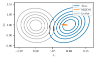
(a) After 100 steps

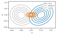
(b) After 36 steps

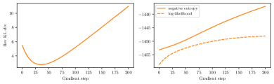
(c) Reverse KL divergence

Figure 1: AR(1) process with $\varphi=0.1$ and $\sigma^{2}=0.99$. Top row illustrates densities of $\Phi(X)$, using fitted 2D Gaussians, at different stages of the descent.

3.2 KL Divergence

Using the reverse KL divergence allows us to analyze the method in examples like the AR(1) model where we have access to the likelihood. If the step size $\gamma$ is small enough, the gradient step (3) is typically contractive and the descent algorithm can be seen as a contractive residual flow. We can therefore write the log-likelihood $\log q_{T}$ as

$$\log q_{T}(x)=\log q_{0}(z)-\sum_{t=0}^{T-1}\log|\det J_{g}(G_{t}(z))|,$$

where $G_{t}$ denotes $t$ compositions of $g$ (with $G_{0}$ being identity), and $G_{T}(z)=x$. When $\Phi$ is efficiently computable, e.g. does not contain a multitude of matrix–vector multiplications with big matrices, and $d$ is not too big, this Jacobian determinant can be computed in reasonable time with automatic differentiation, e.g. using torch.func in PyTorch (Paszke et al., 2019) which allows for vectorized computation.

Going back to the AR(1) example, Figure 1(c) illustrates how the reverse KL divergence starts increasing after a certain number of gradient steps. The marginal increase in expected log-likelihood at each step eventually diminishes as the energy vector approaches the target, whereas the decrease in entropy stays consistent. The figure suggest early stopping as regularization. However, as seen in the figure, even early stopping does not produce a satisfactory distribution. Although it has a higher entropy, the energy distribution is still not centered correctly compared to the true energy distribution. As a result, while there is a trade-off between entropy and log-likelihood, it is a false trade-off in that minimizing the KL divergence leaves us with a poor entropy and a poor log-likelihood.

4 Mean-Field Microcanonical Gradient Descent

The accuracy of the microcanonical approximation is based on the assumption of the concentration of the energy vector $\Phi(X)$ for the true distribution. If the microcanonical set is too large (i.e., too large of a value of $\epsilon$ or too small of a value of $T$), the microcanonical model would include many atypical outcomes that do not satisfy this concentration. On the other hand, the entropy of the microcanonical distribution is the log of the volume of the microcanonical set $\Omega_{\varepsilon}$, and is therefore increasing in the radius $\varepsilon$. Thus, having too small of a radius may ensure no atypical samples are generated, but at the price of a loss of entropy, and will therefore result in a larger KL divergence.

Given that the energy function is appropriate for the distribution, e.g. it is taken to be the sufficient statistics of the distribution as in the AR(1) case, the likelihood increases as the descent progresses and the energy vector approaches the target energy. Conversely, if too many iterates are performed, the energy vectors of the samples will be too close, effectively choosing a radius that is too small.

(a) MGDM

(b) MF-MGDM

Figure 2: Illustration of $\Phi$-pushforward measures of the true distribution in blue centered at the origin, and the approximation in orange. In the regular MGDM, each particle individually seeks to minimize its distance to the origin in energy space, potentially causing a collapse; in the mean-field version, the particles move approximately in parallel in energy space.

This observation leads to our proposition of the mean-field microcanonical gradient descent model (MF–MGDM), where the mass of the initial distribution is pushed towards the target in energy space while attempting to reduce the collapse of the radius of the ball (or similarly the energy variance) and thereby reducing the entropy loss. The principle is illustrated in Figure 2; whereas the regular MGDM (Figure 2(a)) updates each sample individually with the objective of minimizing its energy distance (2) to the target, MF-MGDM (Figure 2(b)) updates several samples simultaneously so that they move towards the target energy in aggregate.

The mean-field concept originates from statistical physics as a tool for studying macroscopic phenomena in large particle systems by averaging over microscopic interactions. In the context of game theory, mean-field games are multiagent problems where each agent has a negligible impact on the others, so that the dynamics of an agent depends on the law of the system. For an $N$-player system, the law is the empirical measure, for which a subclass of systems are those where the dynamics depend on the empirical mean. The mean-field limit is then when $N\to\infty$; see e.g. (Carmona & Delarue, 2018).

A heuristic derivation of the MF–MGDM is the following: Define $\bm{x}=\{x^{(n)}\}_{n=1}^{N}\in\mathcal{X}^{N}$ as a collection of $N$ particles, whereby particle we mean a sample path, and denote the batch mean energy as

$$\bar{\Phi}(\bm{x})=\frac{1}{N}\sum_{i=1}^{N}\Phi(x^{(i)}).$$

We would like to update each particle so that the particles in aggregate moves towards the target energy, i.e. the origin, but requiring that they move in the same direction in energy space. Define this direction as

$$h(\bm{x})=-\gamma\bar{\Phi}(\bm{x}),$$

emulating a force on the batch mean towards the target as illustrated in Figure 2(b). We want to update $\bm{x}$ to $\bm{x}^{\prime}$ so that $\Phi(\bm{x}^{\prime})\approx\Phi(\bm{x})+h(\bm{x})$, which can be seen as an inner optimization problem to minimize the objective $\frac{1}{2}\|\Phi(\bm{x}^{\prime})-(\Phi(\bm{x})+h(\bm{x}))\|$ where we can let $\bm{\xi}_{0}=\bm{x}$ and iteratively perform the update

$$\bm{\xi}_{\tau+1} =\bm{\xi}_{\tau}-\frac{\lambda}{2}\nabla_{\bm{\xi}}\|\Phi(\bm{\xi}_{\tau})-(\Phi(\bm{x})+h(\bm{x}))\|^{2}$$

$$=\bm{\xi}_{\tau}-\lambda J_{\Phi}^{\top}(\bm{\xi}_{\tau})\left[\Phi(\bm{\xi}_{\tau})-(\Phi(\bm{x})+h(\bm{x}))\right]$$

for some number of iterations, where $\lambda$ is the inner step size. Taking only one step in this procedure results in the update rule

$$\bm{x}^{\prime}=\bm{\xi}_{1} =\bm{x}-\lambda J_{\Phi}^{\top}(\bm{x})\left[\Phi(\bm{x})-(\Phi(\bm{x})+h(\bm{x}))\right]$$

$$=\bm{x}-\lambda\gamma J_{\Phi}^{\top}(\bm{x})\bar{\Phi}(\bm{x}).$$

Redefining $\gamma$ as the composite of step lengths in both internal and external optimization, we define the mean-field gradient step as

$$\tilde{g}(\bm{x})=\bm{x}-\gamma J_{\Phi}^{\top}(\bm{x})\bar{\Phi}(\bm{x}).$$ (6)

It is possible to take more steps in the inner iteration, although this would increase the number of times the Jacobian of $\Phi$ has to be computed. From a sampling perspective, it can still be feasible depending on the energy function, since the computation is quite fast, but evaluating the KL divergence can become too costly. Empirically, it seems that one inner iteration is sufficient for the purpose of avoiding collapse, so for the sake of being able to compute KL efficiently, we restrict the model to only one inner iteration.

The MF–MGDM faces two challenges that the regular model does not. The first is that the sampling procedure requires simultaneous generation of multiple samples in order to compute $\bar{\Phi}$. This is solved efficiently by vectorizing the computation of the energy Jacobian in (6). The second challenge is that of computing the entropy, specifically computing the log-determinant of the Jacobian of a gradient step $\tilde{g}$. The issue is that the samples are now coupled, resulting in the Jacobian being one large $Nd\times Nd$ matrix, where the off-diagonal $d\times d$ blocks are non-zero. Naively computing the determinant scales as $\operatorname{\mathcal{O}}(N^{3}d^{3})$ (even keeping it in memory is infeasible), but it is possible to rewrite it on a form that allows $\operatorname{\mathcal{O}}(Nd^{3})$ computation by writing the Jacobian as a sum of a block diagonal and a low-rank matrix, and then using the matrix determinant lemma (see Appendix A).

(a) Energies after 157 steps

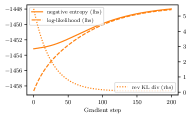
(b) Reverse KL Divergence

Figure 3: MF-MGDM for AR(1) example.

To demonstrate the effect of the mean-field gradient step, we return to the AR(1) example. Figure 3(a) shows the pushforward by $\Phi$ of the initial measure, the final measure after 157 steps, and the true measure. We see now that the final distribution in energy space more closely aligns with that of the true measure, preventing the reduction of entropy observed in the MGDM (see Figure 1(a)). Tracking the reverse KL divergence for each gradient step, Figure 3(b), we see a monotone decrease, avoiding the need for early stopping. If we break up the KL divergence into negative entropy and log-likelihood, we no longer observe an unbounded decrease in entropy. Instead, it stabilizes around a value close to the negative log-likelihood, resulting in a small KL divergence.

In Figure 4, the impact of the choice of $N$ is illustrated. For larger $N$, the estimate $\bar{\Phi}$ of $\mathbb{E}_{q}[\Phi(X)]$ improves, the model also improves in terms of reverse KL divergence. It is also apparent that for $N$ large enough, there are only marginal improvements.

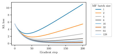
Figure 4: Reverse KL divergence through gradient descent with respect to the true model AR(1) for MF–MGDM with different mean-field batch sizes. The KL estimates are computed from 128 samples.

It is worth pointing out that, although the MF–MGDM is an attempt at maintaining the variance in energy from the initial distribution, this is not guaranteed. For example, with $\Phi(x)\coloneqq\|x\|_{2}^{2}$, we have the update

$$x_{t+1}=x_{t}-2\gamma x_{t}\bar{\Phi}(\bm{x}_{t})=(1-2\gamma\bar{\Phi}(\bm{x}_{t}))x_{t}$$

for an arbitrary particle $x$, so in the mean-field limit,

$$\Phi(x_{t+1})=(1-2\gamma\mathbb{E}_{\mu_{t}}(\Phi(X)))^{2}\Phi(x_{t})$$

and, provided $\mathbb{E}_{\mu_{0}}(\Phi(X))\neq 0$, we obtain

$$\operatorname{Var}_{\mu_{t+1}}(\Phi(X)) =(1-2\gamma\mathbb{E}_{\mu_{t}}(\Phi(X)))^{4}\operatorname{Var}_{\mu_{t}}(\Phi(X))$$

$$<\operatorname{Var}_{\mu_{t}}(\Phi(X)).$$

5 Numerical Experiments

Table 1: Reverse KL divergence for different distributions and approximation models

	ACF eqn. (5)		ScatMean		ScatCov		ScatSpectra
	Reg.	MF	Reg.	MF	Reg.	MF	Reg.	MF
AR$(0.1)$	2.76	0.09	4.24	1.99	5.47	4.01	5.44	2.32
AR$(0.2,-0.1)$	9.44	3.81	17.98	10.55	25.91	14.84	27.33	9.78
AR$(-0.1,0.2,0.1)$	30.04	26.39	20.98	15.18	29.55	18.01	28.46	10.03
CIR$(2^{-1},1,1)$	219.40	214.65	170.63	169.56	121.17	59.21	105.05	30.78
CIR$(2^{-1/2},2^{1/2},1)$	104.49	87.96	182.24	179.52	223.63	204.79	203.44	201.42

To evaluate the performance of this sampling scheme, we apply it to both synthetic and real-world time series, where the latter is taken from applications in financial modeling.

5.1 Synthetic data

To compare the different approximation models on synthetic data, we use time series models that have density functions in closed form, allowing for evaluation of the reverse KL divergence. We generate 10 000 samples of length $1024$ and take the average energy over these samples as target energy, to simulate the idealized setting where the true energy vector is known, avoiding bias. The KL divergence is estimated by generating 128 samples from the respective models, recording the divergence after each gradient step.

The energy functions used are

1. AR(1) approximate sufficient statistics (5) (or equivalently, autocovariance at lags 0 and 1);

2. mean (over time) of second-order scattering transform (with complex modulus as nonlinearity), using filters from the Kymatio package (Andreux et al., 2020);

3. covariance (over time) of second-order scattering transform, augmented with filters shifted by $0$ and $\pi/3$ in the first-order coefficients, and using ReLU of the real part as nonlinearity. Finally, we perform a dimensionality reduction by using principal component analysis (PCA) on transforms applied to Gaussian white noise;

4. scattering spectra from (Morel et al., 2023), taking the modulus of those coefficients which are complex, and thereby ignoring the phase.

These energy functions are applied to two types of synthetic data: autoregressive models of order $p$ ($\text{AR}(p)$) models and Cox–Ingersoll–Ross (CIR) models.

$\text{AR}(p)$

An $\text{AR}(p)$ model with parameters $\varphi_{1},\dots,\varphi_{p}$ and $\sigma$ is a generalization of the AR(1) process in (4) and is defined by the recursion

$$x_{i}=\sum_{j=1}^{p}\varphi_{j}x_{i-j}+\sigma\varepsilon_{i},$$

with white noise $(\varepsilon_{i})_{i}$, and is stationary if the roots of the characteristic polynomial $\pi(z)=1-\sum_{j}\varphi_{j}z^{j}$ are outside the unit circle. In Table 1, the models are denoted AR$(\gamma_{1},\gamma_{2},\dots)$, and $\sigma$ is chosen as to get unit marginal variance.

CIR

The CIR model (Cox et al., 1985) is a diffusion process that is commonly used for modelling short-term interest rates. It is related to the Ornstein–Uhlenbeck process, which can be seen as a continuous version of AR(1), but differs in the way that the diffusion term is scaled by the square root of the rate $r\in\mathbb{R}^{+}$:

$$dr_{t}=\kappa(\theta-r_{t})dt+\sigma\sqrt{r_{t}}dW_{t},$$

where $W$ is a Brownian motion. The process admits a stationary distribution, and the distribution at time $t$ given the value at an earlier time $s<t$ can be written in closed form, allowing for explicit evaluation of the likelihood of a discretization in an autoregressive fashion $\prod_{i}p(r_{i\Delta t}\mid r_{(i-1)\Delta t})$. The distribution of $r_{0}$ can be taken to be the marginal distribution, i.e., a gamma distribution. In the experiments, we let $\Delta t=1$, and the models are identified as CIR$(\kappa,\theta,\sigma)$.

The CIR process is non-negative, so projected gradient descent, described in Appendix B, has to be used when approximating this distribution in the context of MGDM. In addition, the support of the distribution is $\mathbb{R}^{+}$, so given that it exists, the maximum entropy distribution conditioned on the first two moments is the exponential if the mean and standard deviation are equal, otherwise a truncated Gaussian (Dowson & Wragg, 1973).

Results

For each model and energy function, the reverse KL divergence was computed at each step through the descent. The value at the step where minimum divergence was achieved is displayed in Table 1. For every true distribution, we present results also for energy functions that are not necessarily a good choice, given the true model. This is to point out that the MF–MGDM consistently performs at least as well as the MGDM.

The behavior of the divergence through the descent, as well as its constituents entropy and expected log-likelihood, are displayed in Figure 5, using the energy function that best approximates each distribution in accordance with Table 1. Here we see again that less entropy is lost in the mean-field model, and that there is a marginal difference in general between the expected likelihoods of the two models.

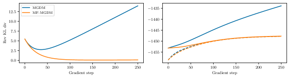
(a) AR$(0.1)$ with ACF as energy.

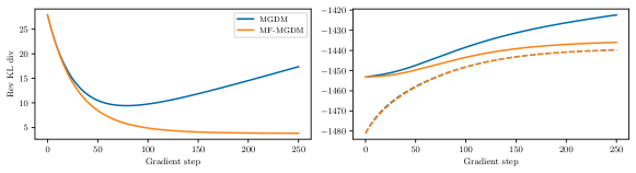
(b) AR$(0.2,-0.1)$ with ACF as energy.

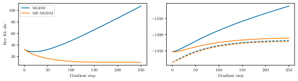
(c) AR$(-0.1,0.2,0.1)$ with scattering spectra as energy.

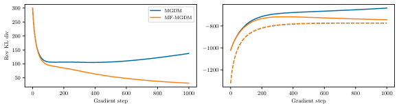
(d) CIR$(2^{-1},1,1)$ with scattering spectra as energy.

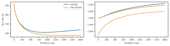
(e) CIR$(2^{-1/2},2^{1/2},1)$ with ACF as energy.

Figure 5: Reverse KL divergence (left), negative entropy (right, solid) and log-likelihood (right, dashed) through the descent. The energy function used for each distribution is the corresponding optimal energy function according to Table 1.

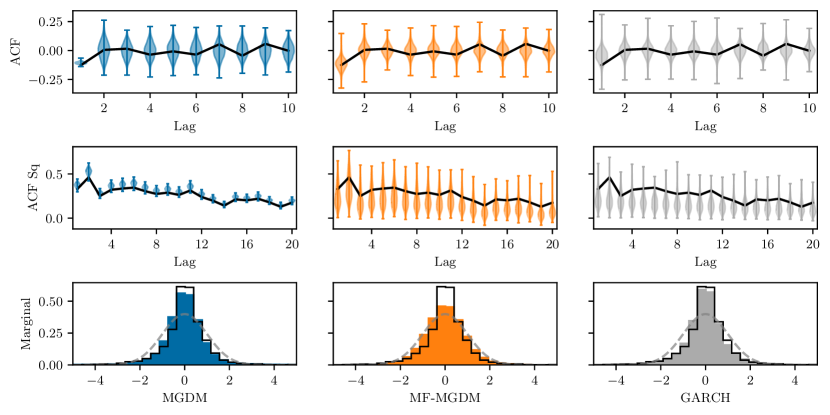
Figure 6: S&P 500 autocorrelation, autocorrelation of the square of the signal, and marginal histogram. The top two rows are violin plots illustrating the empirical marginal density of the statistics for the models, with whiskers indicating min and max. The statistics of the true distribution are in black in all rows. In the bottom row, the dashed gray line is a Gaussian with moments matched to the true data.

Another important difference here is that while MGDM needs to be stopped early to prevent the entropy from collapsing, this is not the case for MF–MGDM. Indeed, we see that the entropy stabilizes after a certain number of steps similarly to the log-likelihood. This is important because in a real-world setting, the true distribution is not known and the reverse KL divergence is not computable, so we cannot reasonably estimate the number of gradient steps to perform in order to balance the entropy loss with the increase of expected log-likelihood. For MF–MGDM, we can run the sampling until convergence without having to worry about this type of overfitting.

5.2 Financial data

We evaluate the model on real financial data, namely the S&P 500 index, and five and ten year synthetic EUR and USD government bonds quoted in yield. For the equity index, daily log-returns are generated, while regular daily returns are used for the rates. To compute the target energy, $2^{12}$ points were used for S&P 500 and USD rates, and $2^{11}$ for EUR rates, corresponding to approximately 16 and 8 years worth of daily data, respectively. For generation, samples of length $2^{10}$, or about 4 years, were produced.

We use stylized features in the energy function, consisting of variance, autocovariance at lag 1, and autocovariance of the squared process for lags 1–20 — statistics that are of interest for financial time series. In Appendix C, we provide results for the scattering covariance as energy. We qualitatively compare the models based on these statistics, as well as marginal distributions, with results displayed in Figure 6 (S&P 500) and Appendix C (rates data). As reference, we also include a GARCH$(1,1)$ model with AR$(1)$ mean process and Student’s t innovations, using maximum likelihood parameters fitted using the Python ARCH package (Sheppard, 2024). The same general behavior is observed here as for the AR$(1)$ example, namely that the MF–MGDM counteracts the overfitting while still producing a good fit of the statistics that the model is conditioned on. The marginal fit, however, which except for the variance is not explicitly optimized for, becomes slightly worse, although it still manages to capture some of the heavy tails.

6 Conclusions

The MGDM provides efficient sampling of high-dimensional distributions, but can suffer from a significant loss of entropy. Propagating too far into the descent is shown to overfit to the target energy that the model is conditioned on, meaning that the variance of the energy for the model is much too small as for what to expect from true distributions. Regularizing by early stopping in the descent mitigates this issue somewhat, but at the price of a worse fit to the true distribution and a larger bias from the initial distribution. The mean-field regularization of the model leverages parallel sampling to mitigate the problem, improving the rate at which entropy is lost without a significant impact on the likelihood fit. Future work will explore better initial distributions and more sophisticated update steps. These will in turn open the door to considering forward KL divergence metrics, removing the need for access to the likelihood of the target distribution.

Impact Statement

This paper presents work whose general goal is to advance the field of machine learning. As such, there are many potential societal consequences of our work, none which must be specifically highlighted here.

Appendix A Appendix – Computing the Jacobian determinant in MF-MGDM

Denote $\tilde{g}^{(n)}$ as the update corresponding to particle $x^{(n)}$:

$$\tilde{g}^{(n)}(\bm{x})=x^{(n)}-\gamma\sum_{k=1}^{K}\nabla\Phi_{k}(x^{(n)})\bar{\Phi}_{k}(\bm{x}).$$

Then the Jacobian w.r.t. a possibly different particle $x^{(m)}$ is, stated by index,

$$\partial_{x^{(m)}_{j}}\tilde{g}^{(n)}_{i}(\bm{x}) =\delta_{m,n}\delta_{i,j}-\gamma\sum_{k}\partial_{x^{(m)}_{j}}\left(\partial_{x^{(n)}_{i}}\Phi_{k}(x^{(n)})\cdot\bar{\Phi}_{k}(\bm{x})\right)$$

$$=\delta_{m,n}\delta_{i,j}-\gamma\sum_{k}\left(\delta_{m,n}\partial_{x^{(n)}_{j}}\partial_{x^{(n)}_{i}}\Phi_{k}(x^{(n)})\cdot\bar{\Phi}_{k}(\bm{x})+\frac{1}{N}\partial_{x^{(n)}_{i}}\Phi_{k}(x^{(n)})\cdot\partial_{x^{(m)}_{j}}\Phi_{k}(x^{(m)})\right),$$

or, stated by block,

$$J_{\tilde{g}^{(n)}}(x^{(m)})=\delta_{m,n}\cdot\left(I-\gamma\sum_{k}H_{\Phi_{k}}(x^{(n)})\bar{\Phi}_{k}(\bm{x})\right)-\frac{\gamma}{N}J_{\Phi}^{\top}(x^{(n)})J_{\Phi}(x^{(m)}).$$

Define the block matrices

$$\mathcal{J}_{\Phi}(\bm{x})=\begin{bmatrix}J_{\Phi}(x^{(1)})&\cdots&J_{\Phi}(x^{(N)})\end{bmatrix}$$

and

$$\mathcal{H}_{\Phi_{k}}(\bm{x})=\operatorname{diag}\left\{H_{\Phi_{k}}(x^{(n)})\right\}_{n=1}^{N}=\begin{bmatrix}H_{\Phi_{k}}(x^{(1)})&&\\ &\ddots&\\ &&H_{\Phi_{k}}(x^{(N)})\end{bmatrix}.$$

Then, the entire Jacobian of $\tilde{g}$ can be expressed as

$$J_{\tilde{g}}(\bm{x})=I-\gamma\sum_{k}\mathcal{H}_{\Phi_{k}}(\bm{x})\bar{\Phi}_{k}(\bm{x})-\frac{\gamma}{N}\mathcal{J}_{\Phi}^{\top}\mathcal{J}_{\Phi}(\bm{x}).$$

Using the matrix determinant lemma, and that

$$I-\gamma\sum_{k}\mathcal{H}_{\Phi_{k}}\bar{\Phi}_{k}$$

is block-diagonal (and thereby also its inverse), the determinant can be reformulated as

$$\det J_{\tilde{g}} =\det\left(I-\gamma\sum_{k}\mathcal{H}_{\Phi_{k}}\bar{\Phi}_{k}-\frac{\gamma}{N}\mathcal{J}_{\Phi}^{\top}\mathcal{J}_{\Phi}\right)$$

$$=\det\left(I-\gamma\sum_{k}\mathcal{H}_{\Phi_{k}}\bar{\Phi}_{k}\right)\det\left(I-\frac{\gamma}{N}\mathcal{J}_{\Phi}\left(I-\gamma\sum_{k}\mathcal{H}_{\Phi_{k}}\bar{\Phi}_{k}\right)^{-1}\mathcal{J}_{\Phi}^{\top}\right)$$

$$=\det\operatorname{diag}\left\{\left(I-\gamma\sum_{k}H_{\Phi_{k}}^{(n)}\bar{\Phi}_{k}\right)\right\}_{n}\det\left(I-\frac{\gamma}{N}\mathcal{J}_{\Phi}\operatorname{diag}\left\{\left(I-\gamma\sum_{k}H_{\Phi_{k}}^{(n)}\bar{\Phi}_{k}\right)^{-1}\right\}_{n}\mathcal{J}_{\Phi}^{\top}\right)$$

$$=\prod_{n}\det\left(I-\gamma\sum_{k}H_{\Phi_{k}}^{(n)}\bar{\Phi}_{k}\right)\det\left(I-\gamma\frac{1}{N}\sum_{n}J_{\Phi}^{(n)}\left(I-\gamma\sum_{k}H_{\Phi_{k}}^{(n)}\bar{\Phi}_{k}\right)^{-1}\left(J_{\Phi}^{(n)}\right)^{\top}\right).$$

Appendix B Appendix – Projected Gradient Descent

In the projected gradient descent used for CIR models, the generating procedure is to update the sample according to the gradient steps while satisfying the constraint of remaining in the positive cone $x\geq 0$. A basic implementation is to alternate between a gradient step and a projection step, where the updated sample is projected onto the feasible set, which in practice amounts to applying a ReLU to the sample after each step; let $g:\mathcal{X}\to\mathcal{X}$ denote the gradient update (regular or mean-field) and $\underline{g}$ the projected gradient update, then

$$\underline{g}=\operatorname{ReLU}{}\circ g.$$

The problem with this definition is that the Jacobian becomes singular if an update is masked by the ReLU, resulting in the determinant being zero. Therefore, we instead use the update

$$\underline{g}_{i}(x)=\begin{cases}g_{i}(x),&g_{i}(x)\geq 0,\\ x_{i},&g_{i}(x)<0.\end{cases}$$

Hence, if a component in the sample is negative after the gradient step $g$, it is replaced by its prior value. In this case, the Jacobian determinant is the same as only looking at the components of the sample that have been updated.

Appendix C Appendix – Additional Plots

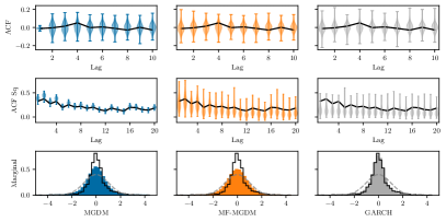
(a) EUR5Y

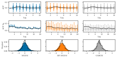
(b) EUR10Y

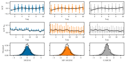
(c) USD5Y

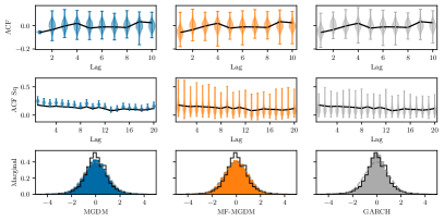
(d) USD10Y

Figure 7: Autocorrelations and marginal histograms as in Figure 6, with same energy function as for S&P 500.

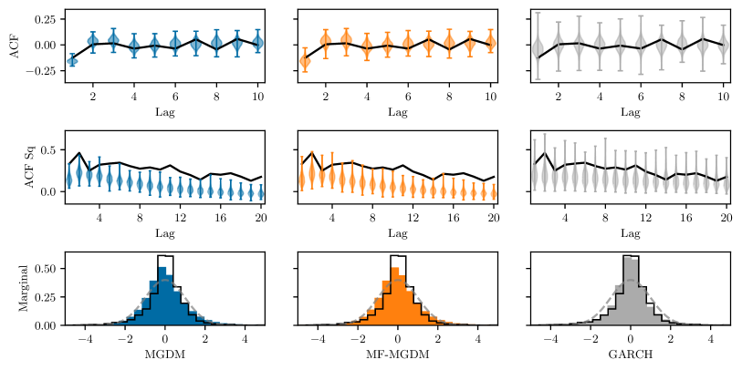
(a) S&P 500

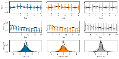
(b) EUR5Y

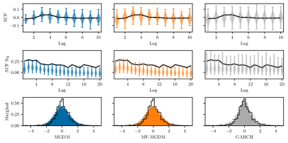
(c) EUR10Y

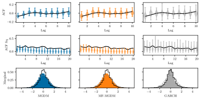
(d) USD5Y

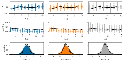
(e) USD10Y

Figure 8: Autocorrelations and marginal histograms as in Figure 6, here using the scattering covariance with phase shifts as described in Section 5.1, but with PCA components now computed using samples from a GARCH process. Since the autocorrelations are not explicitly included in the energy function, the fit is worse. For MGDM, the statistics are not as concentrated as in Figures 6 and 7. The MF–MGDM still provide some improvements, most noticeable in the ACF.

Figure 9: S&P 500 average loss (2) through the descent for the MGDM. The loss can be made arbitrarily small with more descent iterations, implying that the discrepancy in fit of the ACF of the squared signal in Figure 8(a) is not due to getting stuck in a poor local minimum.

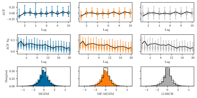
Figure 10: Autocorrelations and marginal histograms with scattering covariance energy as in Figure 8, the initial distribution now coming from a GARCH process as opposed to Gaussian white noise in Figure 8(a). The fit is better for both MGDM and MF-MGDM compared to Fig. 8(a). Together with Figure 9, this shows that the shortcomings in Fig. 8(a) are due to the microcanonical set being too large (i.e., additional momentum constraints are necessary), rather than issues with the decent failing to transport the initial samples to the microcanonical set.

References

- Andreux et al. (2020) Andreux, M., Angles, T., Exarchakis, G., Leonarduzzi, R., Rochette, G., Thiry, L., Zarka, J., Mallat, S., Andén, J., Belilovsky, E., Bruna, J., Lostanlen, V., Chaudhary, M., Hirn, M. J., Oyallon, E., Zhang, S., Cella, C., and Eickenberg, M. Kymatio: Scattering transforms in Python. Journal of Machine Learning Research, 21(60):1–6, 2020.
- Andén et al. (2019) Andén, J., Lostanlen, V., and Mallat, S. Joint time–frequency scattering. IEEE Transactions on Signal Processing, 67(14):3704–3718, 2019.
- Auclair et al. (2023) Auclair, C., Allys, E., Boulanger, F., Béthermin, M., Gkogkou, A., Lagache, G., Marchal, A., Miville-Deschênes, M.-A., Régaldo-Saint Blancard, B., and Richard, P. Separation of dust emission from the cosmic infrared background in Herschel observations with wavelet phase harmonics. Astronomy & Astrophysics, 681:A1, 2023.
- Brochard et al. (2022) Brochard, A., Zhang, S., and Mallat, S. Generalized rectifier wavelet covariance models for texture synthesis. In International Conference on Learning Representations, 2022.
- Bruna & Mallat (2013) Bruna, J. and Mallat, S. Invariant scattering convolution networks. IEEE Transactions on Pattern Analysis and Machine Intelligence, 35(8):1872–1886, 2013.
- Bruna & Mallat (2019) Bruna, J. and Mallat, S. Multiscale sparse microcanonical models. Mathematical Statistics and Learning, 1(3):257–315, 2019.
- Buehler et al. (2020) Buehler, H., Horvath, B., Lyons, T., Perez Arribas, I., and Wood, B. A data-driven market simulator for small data environments. arXiv preprint arXiv:2006.14498, 2020.
- Carmona & Delarue (2018) Carmona, R. and Delarue, F. Probabilistic theory of mean field games with applications I-II. Springer, 2018.
- Cheng et al. (2023) Cheng, S., Morel, R., Allys, E., Ménard, B., and Mallat, S. Scattering spectra models for physics. arXiv preprint arXiv:2306.17210, 2023.
- Cover & Thomas (2006) Cover, T. M. and Thomas, J. A. Elements of Information Theory. John Wiley & Sons, Inc., 2nd edition, 2006. ISBN 978-0-471-24195-9.
- Cox et al. (1985) Cox, J. C., Ingersoll, J. E., and Ross, S. A. A theory of the term structure of interest rates. Econometrica, 53(2):385, 1985. doi: 10.2307/1911242.
- Dowson & Wragg (1973) Dowson, D. and Wragg, A. Maximum-entropy distributions having prescribed first and second moments. IEEE Transactions on Information Theory, 19(5):689–693, 1973.
- Du & Mordatch (2019) Du, Y. and Mordatch, I. Implicit generation and generalization in energy-based models. arXiv preprint arXiv:1903.08689, 2019.
- Eickenberg et al. (2017) Eickenberg, M., Exarchakis, G., Hirn, M., and Mallat, S. Solid harmonic wavelet scattering: Predicting quantum molecular energy from invariant descriptors of 3d electronic densities. In Advances in Neural Information Processing Systems, volume 30, 2017.
- Ellis et al. (2000) Ellis, R. S., Haven, K., and Turkington, B. Large deviation principles and complete equivalence and nonequivalence results for pure and mixed ensembles. Journal of Statistical Physics, 101(5):999–1064, 2000.
- Geman & Geman (1984) Geman, S. and Geman, D. Stochastic relaxation, Gibbs distributions, and the Bayesian restoration of images. IEEE Transactions on Pattern Analysis and Machine Intelligence, 6(6):721–741, 1984.
- Jaynes (1957) Jaynes, E. T. Information theory and statistical mechanics. Physical Review, 106(4):620–630, 1957.
- Lanford (1975) Lanford, O. E. Time evolution of large classical systems. In Moser, J. (ed.), Dynamical Systems, Theory and Applications, pp. 1–111. Springer, Berlin, Heidelberg, 1975.
- Leonarduzzi et al. (2019) Leonarduzzi, R., Rochette, G., Bouchaud, J.-P., and Mallat, S. Maximum-entropy scattering models for financial time series. In IEEE International Conference on Acoustics, Speech and Signal Processing (ICASSP), pp. 5496–5500, 2019.
- Lostanlen et al. (2021) Lostanlen, V., El-Hajj, C., Rossignol, M., Lafay, G., Andén, J., and Lagrange, M. Time–frequency scattering accurately models auditory similarities between instrumental playing techniques. EURASIP Journal on Audio, Speech, and Music Processing, 2021(1):3, 2021.
- Lyons (2014) Lyons, T. Rough paths, signatures and the modelling of functions on streams. arXiv preprint arXiv:1405.4537, 2014.
- Mallat (2012) Mallat, S. Group invariant scattering. Communications on Pure and Applied Mathematics, 65(10):1331–1398, 2012.
- Mallat (2016) Mallat, S. Understanding deep convolutional networks. Philosophical Transactions of the Royal Society A: Mathematical, Physical and Engineering Sciences, 374(2065), 2016.
- Mallat et al. (2019) Mallat, S., Zhang, S., and Rochette, G. Phase harmonic correlations and convolutional neural networks. Information and Inference: A Journal of the IMA, 9(3):721–747, 2019.
- Morel et al. (2023) Morel, R., Rochette, G., Leonarduzzi, R., Bouchaud, J.-P., and Mallat, S. Scale dependencies and self-similar models with wavelet scattering spectra. Available at SSRN 4516767, 2023.
- Ni et al. (2021) Ni, H., Szpruch, L., Sabate-Vidales, M., Xiao, B., Wiese, M., and Liao, S. Sig-Wasserstein GANs for time series generation. arXiv preprint arXiv:2111.01207, 2021.
- Oyallon et al. (2019) Oyallon, E., Zagoruyko, S., Huang, G., Komodakis, N., Lacoste-Julien, S., Blaschko, M., and Belilovsky, E. Scattering networks for hybrid representation learning. IEEE Transactions on Pattern Analysis and Machine Intelligence, 41(9):2208–2221, 2019.
- Papamakarios et al. (2021) Papamakarios, G., Nalisnick, E., Rezende, D. J., Mohamed, S., and Lakshminarayanan, B. Normalizing flows for probabilistic modeling and inference. Journal of Machine Learning Research, 22(1):2617–2680, 2021.
- Paszke et al. (2019) Paszke, A., Gross, S., Massa, F., Lerer, A., Bradbury, J., Chanan, G., Killeen, T., Lin, Z., Gimelshein, N., Antiga, L., Desmaison, A., Kopf, A., Yang, E., DeVito, Z., Raison, M., Tejani, A., Chilamkurthy, S., Steiner, B., Fang, L., Bai, J., and Chintala, S. PyTorch: An Imperative Style, High-Performance Deep Learning Library. In Advances in Neural Information Processing Systems, pp. 8024–8035, 2019.
- Sheppard (2024) Sheppard, K. bashtage/arch: Release 6.3, 2024.
- Touchette (2015) Touchette, H. Equivalence and nonequivalence of ensembles: Thermodynamic, macrostate, and measure levels. Journal of Statistical Physics, 159(5):987–1016, 2015.
- Warrick et al. (2020) Warrick, P. A., Lostanlen, V., Eickenberg, M., Andén, J., and Homsi, M. N. Arrhythmia classification of 12-lead electrocardiograms by hybrid scattering-LSTM networks. In 2020 Computing in Cardiology, pp. 1–4, 2020.
- Zhang & Mallat (2021) Zhang, S. and Mallat, S. Maximum entropy models from phase harmonic covariances. Applied and Computational Harmonic Analysis, 53:199–230, 2021.