Parameter Constraints on Traversable Wormholes within Beyond Horndeski Theories through Quasi-Periodic Oscillations
Abstract
Hunting compact astrophysical objects such as black holes and wormholes, as well as testing gravity theories, are important issues in relativistic astrophysics. In this sense, theoretical and observational studies of quasiperiodic oscillations (QPOs) observed in (micro)quasars become helpful in exploring their central object, which can be a black hole or a wormhole. In the present work, we study the throat properties of traversable wormholes beyond Horndeski theory. Also, we investigate the circular motion of test particles orbiting the wormhole. We analyze the test particle’s effective potential and angular momentum for circular orbits. Frequencies of radial and vertical oscillations of the particles around stable circular orbits have also been studied and applied in explaining the quasiperiodic oscillations mechanism in the relativistic precession (RP) model. Finally, we obtain constraint values for the parameters of Horndeski gravity and the mass of the wormhole candidates using QPOs observed in the microquasars GRO J1655-40, GRS 1915+105 & XTE J1550-564 and at the center of Milky Way galaxy through Monte-Carlo-Markovian-Chain (MCMC) analyses.
pacs:
04.50.-h, 04.40.Dg, 97.60.GbI Introduction
While General Relativity (GR) has been well tested in both weak and strong gravity regimes and is in accordance with all current observations Will (2006, 2018), it also leaves us with several challenging open problems associated, in particular, with its quantization and the dark sector in cosmology. This has caused a flurry of interest in alternative theories of gravity in recent years (see e.g., Berti et al. (2015); Akrami et al. (2021)).
Certainly, any viable alternative theory of gravity must adhere to solar system constraints. However, in the strong gravity sector, current observational data are still less accurate, calling for future observations to test new theoretical predictions. In our current multi-messenger era much insight into alternative theories of gravity can be gained from (future) gravitational wave observations as well as from the observations in the full electromagnetic spectrum and particle detections Abbott et al. (2017).
Among the numerous alternative theories of gravity Horndeski theories Horndeski (1974); Deffayet and Steer (2013) have been very attractive, since they involve only additional scalar degrees of freedom, leading to a set of second-order generalized Einstein-scalar field equations. Thus these theories are free of Ostrogradski instabilities. Indeed, Horndeski theories provide interesting predictions for black holes and neutron stars Berti et al. (2015) and also for cosmology Akrami et al. (2021).
A new interesting class of alternative theories of gravity that extends the Horndeski theories was introduced in Gleyzes et al. (2015a). Whereas their equations are higher order in derivatives, the propagating degrees of freedom still possess second-order equations, making them free from Ostrogradski instabilities, as well. Such beyond Horndeski Gleyzes et al. (2015a) and DHOST theories Langlois and Noui (2016); Crisostomi et al. (2016a) are based on “degenerate” Lagrangians, whose kinetic matrix cannot be inverted, and the ensuing constraints result in a reduced number of physical degrees of freedom. Interestingly, when starting from Horndeski theories, beyond Horndeski theories can be generated with certain types of transformations Gleyzes et al. (2015b); Crisostomi et al. (2016b, a).
A well-motivated set of Horndeski theories are the Einstein-scalar-Gauss-Bonnet gravities. Such theories arise, for instance, in the low-energy regime of string theory Gross and Sloan (1987); Metsaev and Tseytlin (1987). Although they always involve a scalar field, this field can be coupled in a variety of ways, yielding rather different phenomenology when applied to compact objects and cosmology. This allows us to obtain constraints on the respective coupling constants.
One of the most interesting predictions of the gravitational theories is wormholes. In general relativity, they cannot exist without violating the energy conditions. However, in some modified theories of gravity such as Gauss-Bonnet gravity or the f(R) theories the wormhole throat can be supported by the gravitational interaction itself without requiring the presence of exotic matter Hochberg (1990); Fukutaka et al. (1989); Ghoroku and Soma (1992); Lobo and Oliveira (2009); Kanti et al. (2011, 2012); Antoniou et al. (2020); Ibadov et al. (2020). In these theories, wormholes are viable alternatives of black holes. They could play a significant astrophysical role if their existence is confirmed observationally.
Searching for macroscopic wormholes alongside other exotic compact objects is currently one of the major goals of the astrophysical missions testing gravity in the strong field regime. Therefore, many theoretical works focus on studying their phenomenology. Studies of the quasinormal modes in wormhole geometries include Blázquez-Salcedo et al. (2018); Azad et al. (2023); González et al. (2022); Churilova et al. (2021). In the electromagnetic spectrum phenomenological effects arise primarily due to the specifics of the gravitational lensing in the wormhole spacetime Nedkova et al. (2013); Gyulchev et al. (2018); Bambi (2013); Tsukamoto et al. (2012); Wielgus et al. (2020); Huang et al. (2023) and the properties of the accretion process in their vicinity Chakraborty and Pradhan (2017); Harko et al. (2009); Zhou et al. (2016). Thus, it was demonstrated that wormholes can lead to a non-trivial morphology of the observable image of the accretion disk Paul et al. (2020); Vincent et al. (2021). In addition to the primary disk image, they produce a series of bright rings at its center that proved to represent an observational signature of a rather general class of horizonless compact objects Gyulchev et al. (2020, 2021); Eichhorn et al. (2023). Polarized emission from the accretion disk around the wormholes may further possess a distinctive twist of the polarization vector around the image Delijski et al. (2022). Thus, provided that we can observe radiation reaching through the throat of the wormhole, the properties of its linear polarization can serve as a distinctive signature for detecting traversable wormholes.
A possible way to test the spacetime of compact gravitational objects such as black holes and wormholes is by using spectrometrical analyses of radiation of accreting matter around them. However, the gravity of black holes in binary systems plays a crucial role in deriving all the radiation processes in the surrounding accretion disk. Astrophysical phenomena known as QPOs are found using Fourier analyses of the noisy continuous X-ray data from the accretion disk in (micro)quasars (containing black holes or neutron stars and companion stars as binary systems) Stella and Vietri (1998); Stella et al. (1999), and they are classified as high frequency (HF) when the peak frequencies are about 0.1 to 1 kHz and low frequency (LF) when the frequencies are less than about 0.1 kHz Stella et al. (1999). Although high-accuracy measurements of QPO frequencies have been observed in binary systems, no exact and unique physical mechanisms for QPOs have been found yet. This problem is currently under active discussion to test gravity theories and measure the inner edge of the accretion disc. Such measurements may provide valuable information about ISCO radii and black hole parameters. In our previous studies Rayimbaev et al. (2021a, b, 2022a, 2022b, 2022c, 2022d, 2023a); Murodov et al. (2023); Rayimbaev et al. (2023b, c); Qi et al. (2023), we have shown that studies of the QPO orbit may help to determine the ISCO radius which lies near the orbit since the distance between these orbits is in the order of the error of measurements using the relativistic precision model.
The quasi-periodic oscillations in wormhole spacetimes were previously studied within the geodesic models in Deligianni et al. (2021a, b); De Falco et al. (2021); Stuchlík and Vrba (2021a, b); De Falco (2023). Using the resonance models, it was demonstrated that twin peak oscillations can be described by a more diverse resonance structure compared to black holes Deligianni et al. (2021a, b). Wormhole geometries may allow for parametric and forced resonances of lower order which produce more significant observable signals. In addition, resonances may be excited in an arbitrarily close vicinity of the wormhole throat, further amplifying the signals and allowing probes to be placed deep inside the gravitational field of the compact object.
The possibility to explain the observed quasi-periodic oscillations of astrophysical X-ray sources through an underlying wormhole spacetime was investigated in Stuchlík and Vrba (2021a). Using the Simpson-Visser metric, which interpolates between different compact object geometries, including wormholes, the QPOs were modeled as parametric resonances between the epicyclic frequencies. The results were used to fit the observational data for microquasars and active galactic nuclei with available independent mass measurements.
The aim of this paper is to investigate further the compatibility of the wormhole geometry with the properties of certain X-ray sources using QPO measurements. We explore a traversable wormhole spacetime that arises as an exact solution within a beyond Horndeski gravitational theory Bakopoulos et al. (2022) and interpret the twin peak frequencies applying the geodesic precession model. Using a Markov Chain Monte Carlo algorithm we fit the theoretical predictions for the QPO frequencies to the observational data for the microquasars GRO J1655-40, GRS 1915+105, and XTE J1550-564 and the galactic target Sgr A*. In this way, we provide constraints on the parameters of the beyond Horndeski gravitational theory and the possible wormhole geometry.
The paper is organized as follows. In Section II we review the wormhole solution in the beyond Horndeski theory, which we explore. In sections III and IV we study the circular timelike geodesics in the equatorial plane and derive the epicyclic frequencies. In Section V we describe the QPO frequencies using the geodesic precession model investigating their properties. In section VI we perform a fit of the observational data for the microquasars GRO J1655-40, GRS 1915+105, and XTE J1550-564 and the center of our galaxy Sgr A* constraining the parameters of the gravitational theory as well as the wormhole mass and the QPOs excitation radius. In the last section, we present our conclusions.
II Beyond Horndeski Wormholes
The traversable beyond Horndeski wormhole solutions obtained by Bakopoulos et al. Bakopoulos et al. (2022) are based on the black hole seed solution of Lu-Pang Lu and Pang (2020); Hennigar et al. (2020); Fernandes et al. (2020) in a Horndeski theory defined by the functions
where , represents the Horndeski scalar field, and is the Horndeski coupling constant, Clifton et al. (2020); Charmousis et al. (2022); Bakopoulos et al. (2022).
This black hole seed solution is static and spherically symmetric with metric parametrization
| (1) |
where and . The metric functions and scalar field function are Lu and Pang (2020)
| (2) | |||||
| (3) |
respectively, and the prime indicates a partial derivative with respect to . Note, that this corresponds to the asymptotically flat branch of the seed solution Lu and Pang (2020). The parameter then corresponds to the mass of the seed black hole, and the radius of the outer horizon is given by . For , the seed solution becomes a naked singularity.
The Horndeski seed solution is turned into a beyond Horndeski solution by a disformal transformation of the metric (see, e.g., Zumalacárregui and García-Bellido (2014); Crisostomi et al. (2016b); Ben Achour et al. (2016a, b); Bakopoulos et al. (2022))
| (4) |
where the new beyond Horndeski metric is obtained from the seed Horndeski metric by making use of a disformability function leading toBakopoulos et al. (2022)
| (5) | |||||
| (6) | |||||
| (7) | |||||
| (8) |
As shown by Bakopoulos et al. Bakopoulos et al. (2022) the crucial transformation function needs to satisfy certain constraints to obtain a traversable wormhole solution from the seed. In particular, the radial coordinate at the throat , where has a root, should be chosen such that , and for . Moreover, for to preserve asymptotic flatness. These constraints led to the choice Bakopoulos et al. (2022)
| (9) | |||||
since
| (10) |
and is a new dimensionless positive parameter.
The three constants , , and entering the wormhole solutions may not all be chosen independently, but they have to satisfy constraints. The physical requirement, that be the wormhole throat translates to . Eq. (9) then yields
| (11) |
Moreover, it is required that
| (12) |
since for would move to infinity and for , Bakopoulos et al. (2022). Inserting the metric function in eq. (11) and solving for the throat radius one obtains the relation
| (13) |
and since the radicand in eq. (13) should not become negative, this leads to the bound Bakopoulos et al. (2022)
| (14) |
Also, we will take into account observational constraints on the Horndeski coupling constant obtained, in particular, from inflation in the early universe and binary systems with black holes Clifton et al. (2020); Charmousis et al. (2022).
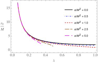
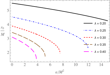
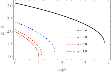
The behavior of the wormhole throat as a function of the solution parameters is presented in Fig. 1. We see that its location moves to smaller values of the radial coordinate when any of the parameters or increases.
We should note that the radial coordinate does not cover the wormhole spacetime completely. By definition it ranges from the wormhole throat, where we have a coordinate singularity, to representing one of the asymptotic ends of the spacetime. In order to define a global coordinate system that also covers the second asymptotic end, we should extend the radial coordinate through the wormhole throat. This is possible for example by defining the coordinate . It describes two identical spacetime regions glued at the throat of the wormhole , taking negative or positive values in each of them. The asymptotic ends correspond to , respectively, and the wormhole throat is located at .
III Circular motion around a traversable wormhole in beyond Horndeski theory
In this section, we first investigate the circular motion of electrically neutral test particles in the spacetime of a traversable wormhole in beyond Horndeski theory, together with the energy and angular momentum of test particles in stable circular orbits.
III.1 Equations of motion
First, we start deriving the equations of motion using the following Lagrangian for test particles,
| (15) |
where is the mass of the particle. We obtain the integrals of motion such as the specific energy , and angular momentum of the particles in the following form
| (16) |
Spherical symmetry allows us to set and . The equation for the radial motion of the test particles can then be obtained using the normalization condition, and taking into account the integrals of the motion (16)
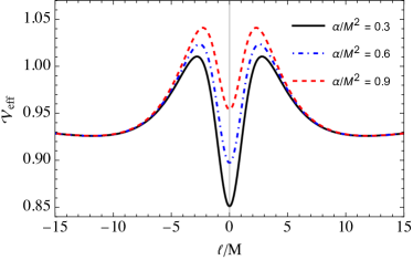
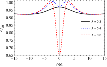
In Fig. 2, we show the dependence of the effective potential on the radial coordinate , where , for various values of and . In the top panel, we show the effective potential for and several values of . We find that an increase in causes an increase in the effective potential for small values of the radial coordinate . The gravitational effect of the parameter becomes less pronounced for large values , leading only to small variations in the effective potential.
In the bottom panel, we illustrate the effect of on the effective potential for the case . We see that variation of the parameter can lead to modification of the qualitative behavior of the effective potential. For larger values of we observe that the effective potential possesses two maxima located symmetrically on both sides of the wormhole throat and a minimum at the throat. Decreasing the parameter , the two maxima approach the throat and at some critical value of they reach it merging into a single maximum and causing the minimum of the effective potential to disintegrate. This transition has an impact on the qualitative behavior of the timelike geodesics in the wormhole spacetime. While the first configuration allows for bound particle orbits in the vicinity of the wormhole throat, the second one possesses only a single unstable circular orbit located at the throat.
Next, we explore the stable circular orbits of test particles around the traversable wormhole using the standard conditions
| (19) |
The expressions for the angular momentum and the energy of test particles corresponding to circular orbits take the form
| (20) |
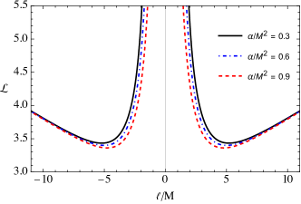
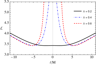
The dependence of the angular momentum on the radial coordinate is shown in Fig. 3 for different values of the parameters and . The figure shows that the angular momentum decreases slightly with an increase of both the parameters and . However, at distances less than about, the angular momentum increases as increases. Also, the angular momentum at increases as increases.
IV Fundamental frequencies of test particles
Fundamental frequencies around astrophysical compact gravitational objects, such as black holes and wormholes, are related to the motion of matter or particles in the spacetime of the objects in the strong gravitational field regime. These frequencies can be used to probe the properties of black holes and wormholes, such as their mass, spin, and gravity parameters. Now we investigate fundamental frequencies of test particles orbiting a traversable wormhole in beyond Horndeski theory. We start by calculating the angular velocity of the test particles in Keplerian orbits and the frequencies of the radial and vertical oscillations of the particles around the stable circular orbits.
The angular velocity of the test particles around central compact gravitating objects in circular orbits is called Keplerian frequency and is defined as where the dot denotes differentiation with respect to the affine parameter along the geodesic. The expression for the Keplerian frequency in the spacetime around a traversable wormhole in beyond Horndeski theory takes the following form
| (21) |
The harmonic oscillations of the test particles around the central massive object are a result of the balance between the gravitational force of the object and the inertia of the test particle.
In fact, when a test particle is placed on a stable circular orbit around the object, it is subject to a centripetal force that is directed towards the object. This force is balanced by the gravitational force of the object, which is directed towards the center of it. If the test particle is slightly perturbed from its circular orbit, such as and , it will experience a restoring force that will tend to bring it back to its original orbit. This restoring force is a result of the gradient of the gravitational field. The restoring force can be resolved into two components: a radial component and a vertical component. The radial component of the restoring force is responsible for the radial oscillations of the test particle, while the vertical component of the restoring force is responsible for the vertical one.
Now, here, we assume test particles orbiting a traversable wormhole along stable circular orbits which oscillate along the radial and the vertical directions. The following equations can evaluate the frequencies of the radial and the vertical oscillations Bardeen et al. (1972):
| (22) |
where
| (23) | |||
| (24) |
are the radial and vertical frequencies, respectively.
After some simple algebraic calculations, one may easily obtain the expressions for the frequencies,
| (26) |
It is worth noting that, in our further analysis, we express all the frequencies in the unit of Hz, i.e. we obtain for the epicyclic frequencies , where is the speed of light in vacuum, and is the gravitational Newtonian constant.
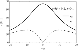

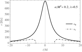

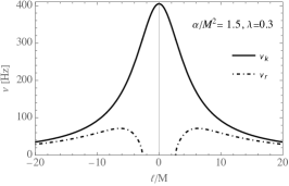

In Fig. 4 we demonstrate the behavior of the profiles of the Keplerian and the radial oscillation frequencies, when we vary the parameters and . It is seen that when and , and and the radial frequency goes to zero at . In fact, the radial oscillations equal zero at the ISCO. This means that the ISCO of the particles coincides with the throat of the wormhole. As the parameter increases, the ISCO goes far from the wormhole throat.
It is also observed that the effect of the coupling parameter is visible near , and an increase of causes a slight decrease in the Keplerian frequency values. However, the parameter increases it.
V Quasi-Periodic Oscillation Frequencies
Astrophysical compact objects, such as black holes and wormholes, do not emit electromagnetic radiation themselves. However, they do cause the curvature of spacetime, which in turn affects the motion of matter in their vicinity. This motion can generate electromagnetic radiation, which can be observed in the form of an accretion disk.
Quasi-periodic oscillations (QPOs) are a type of variability observed in the electromagnetic radiation from accretion disks. QPOs are characterized by their frequency, which can be either high (HF QPOs) or low (LF QPOs). HF QPOs have frequencies in the range of 0.1 to 1 kHz, while LF QPOs have frequencies below 0.1 kHz. QPOs have been observed in the electromagnetic radiation from accretion disks around various astrophysical objects, including black holes, neutron stars, white dwarfs, and their binary systems Ingram et al. (2016). The origin of QPOs is not fully understood, but they are thought to be related to the dynamics of the accretion disk. The study of QPOs can provide insights into the physics of accretion disks and the properties of the compact objects they orbit. For example, the frequency of HF QPOs has been linked to the size of the inner region of the accretion disk, which is in turn related to the mass and spin of the compact object. Consequently, one can conclude that QPOs are a valuable tool for studying the physics of accretion disks and the properties of the compact objects they orbit.
QPOs observed in low-mass X-ray binaries (LMXBs) are thought to be produced by a mechanism different from that observed in other astrophysical objects. This is because LMXBs contain neutron stars that have strong magnetic fields. The magnetic field of a neutron star can interact with the accretion disk in a way that produces QPOs. The source of the electromagnetic radiation in the accretion disk is thought to be the oscillation of test-charged particles. These particles radiate with the same frequency as their oscillation frequency. The relativistic precession (RP) model explains the existence of QPOs due to the quasiharmonic oscillations of charged particles in the radial and angular directions around black holes and wormholes.
In the RP model, the upper frequency of a twin-peaked QPO is equal to the orbital frequency of the particle, while the lower frequency is equal to the difference between the orbital frequency and the radial oscillation frequency. In other words, the upper and lower frequencies of a QPO with twin peaks are given by: and , where, and are the upper and lower frequencies, respectively, and is the orbital frequency and is the radial oscillation frequency.
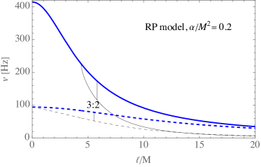
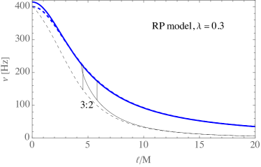
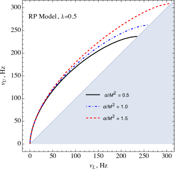
Figure 5 presents the radial dependence of the upper and lower frequencies of twin QPOs with blue and black lines, respectively. In the upper panel, the parameter is fixed as and the solid line corresponds to and the dashed line to . It is observed from this panel that an increase in the parameter causes a decrease in the upper and lower frequencies, and the QPO orbit, with the frequency ratio of 3:2, slightly shifts out. In the bottom panel, we specify the solid line for and the dashed one for cases by fixing the parameter . It is seen that an increase of reduces slightly near the wormhole throat (up to about ), and, at far distances, its effect is invisible. However, the effects of the parameter on the lower frequencies are sufficient.
We perform an analysis of the relationships between the upper and lower frequencies of the twin QPOs for different values of and in Fig. 6.
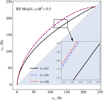
In the left panel, we show the relationships for different values of in , and in the right panel, the relationships are given for different values of by fixing . It is obtained that one can observe an increase in the highest values of upper and lower frequencies corresponding to those generated at ISCO, due to an increase in . However, the highest value does not change in the variation of and it only depends on . From the right panel, it is also seen that the frequency ratio increases slightly with increasing .
VI Constraints on the wormhole mass in beyond Horndeski theory
In this section, we investigate four X-ray binary systems and endeavor to derive constraints on the parameters associated with our wormhole model within the beyond Horndeski theory framework. This will be achieved by analyzing the QPOs’ data. Celestial objects of interest include , GRO J1655-40, GRS 1915 + 10, and XTE 1550-564. Finally, we shall present the best-fit values within the parameter space, which have been obtained through the utilization of a Markov Chain Monte Carlo (MCMC) code analysis.
| GRO J1655-40 | GRS 1915+105 | XTE J1550-564 | ||
|---|---|---|---|---|
| Abramowicz et al. (2004) | 6.036.57 Kološ et al. (2020) | Remillard and McClintock (2006) | 8.49 9.71 Remillard et al. (2002); Orosz et al. (2011) | |
| (Hz) | Abramowicz et al. (2004) | 451 5 Kološ et al. (2020) | 168 3 Remillard and McClintock (2006) | 276 3 Remillard et al. (2002) |
| (Hz) | Abramowicz et al. (2004) | 298 4 Kološ et al. (2020) | 113 5 Remillard and McClintock (2006) | 184 5 Remillard et al. (2002) |
Markov Chain Monte Carlo (MCMC) analysis was performed using the Python library emcee Foreman-Mackey et al. (2013) to determine constraints on the wormhole parameters in our study. We employed the relativistic precession (RP) model in our analysis.
The posterior can be defined as in the reference Liu et al. (2023):
| (27) |
where is the prior and is the likelihood. The priors are set to be Gaussian priors within boundaries, i.e.,
| (28) |
where for the parameters and are their corresponding sigmas. Here we use the notation and is the normalized radial location of the 3:2 resonance. We take the prior values of the parameters of the wormhole, as presented in Table 2.
In light of the upper and lower frequency data obtained in Section V, our MCMC analysis is structured to utilize two distinct datasets. The central component of this analysis is the likelihood function, denoted as , and can be expressed as follows:
| (29) |
wherein characterizes the likelihood associated with the upper-frequency data, given by:
| (30) |
On the other hand, signifies the likelihood attributed to the lower frequency data, expressed as:
| (31) |
Here runs from 1 to an arbitrary integer, implying the number of measured upper and/or lower frequencies, and represent the observed results for the upper and lower frequencies, denoted as and , respectively. Additionally, and correspond to their respective theoretical predictions. Furthermore, within these expressions, represents the statistical uncertainties associated with the given quantities.
| Parameters | GRO J1655-40 | GRS 1915+105 | XTE J1550-564 | |||||
|---|---|---|---|---|---|---|---|---|
| 6.307 | 0.066 | 12.41 | 0.62 | 9.10 | 0.61 | |||
| 1.20 | 0.29 | 1.20 | 0.090 | 1.20 | 0.09 | 1.20 | 0.12 | |
| 0.50 | 0.15 | 0.45 | 0.080 | 0.20 | 0.12 | 0.23 | 0.05 | |
| 6.07 | 0.35 | 5.68 | 0.115 | 4.84 | 0.35 | 4.95 | 0.35 | |
| Parameters | GRO J1655-40 | GRS 1915+105 | XTE J1550-564 | |
|---|---|---|---|---|
VII Conclusion: Results and Discussion
Throughout this work, we have investigated the dynamics and oscillation of test particles together with the applications to QPOs observed near traversable wormholes in beyond Horndeski gravity theories. The following main results are found:
-
•
The wormhole throat decreases with the increase of the Horndeski parameters and .
-
•
The angular momentum decreases slightly with an increase in both the parameters and . However, at distances less than about, the angular momentum increases as increases.
-
•
An increase in causes an increase in the effective potential. However, the gravitational effect of the parameter disappears at .
-
•
Once we have & , the ISCO of the particles coincides with the wormhole throat. As the parameter increases, the ISCO goes far from the wormhole throat.
-
•
An increase in the parameter causes a decrease in the upper and lower frequencies, and the QPO orbit with the frequency ratio 3:2, slightly shifts out.
-
•
An increase of reduces slightly near the wormhole throat (up to about ), and, at far distances (about ), its effect is invisible.
-
•
One can observe an increase in the highest values of the upper and lower frequencies corresponding to those generated at ISCO, due to an increase in .
-
•
However, the highest value does not change in the variation of and it only depends on , also the frequency ratio increases slightly with increasing .
-
•
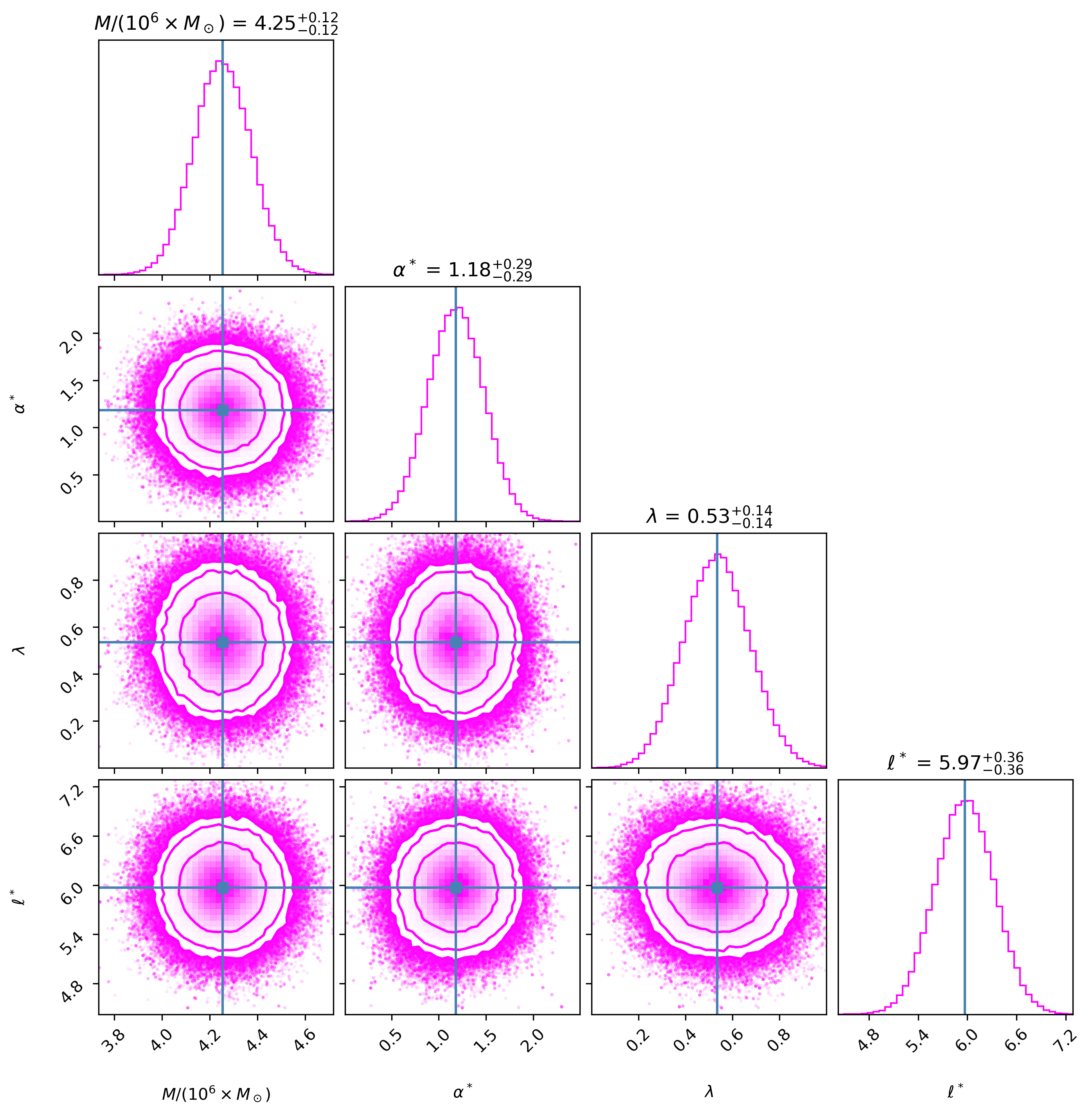
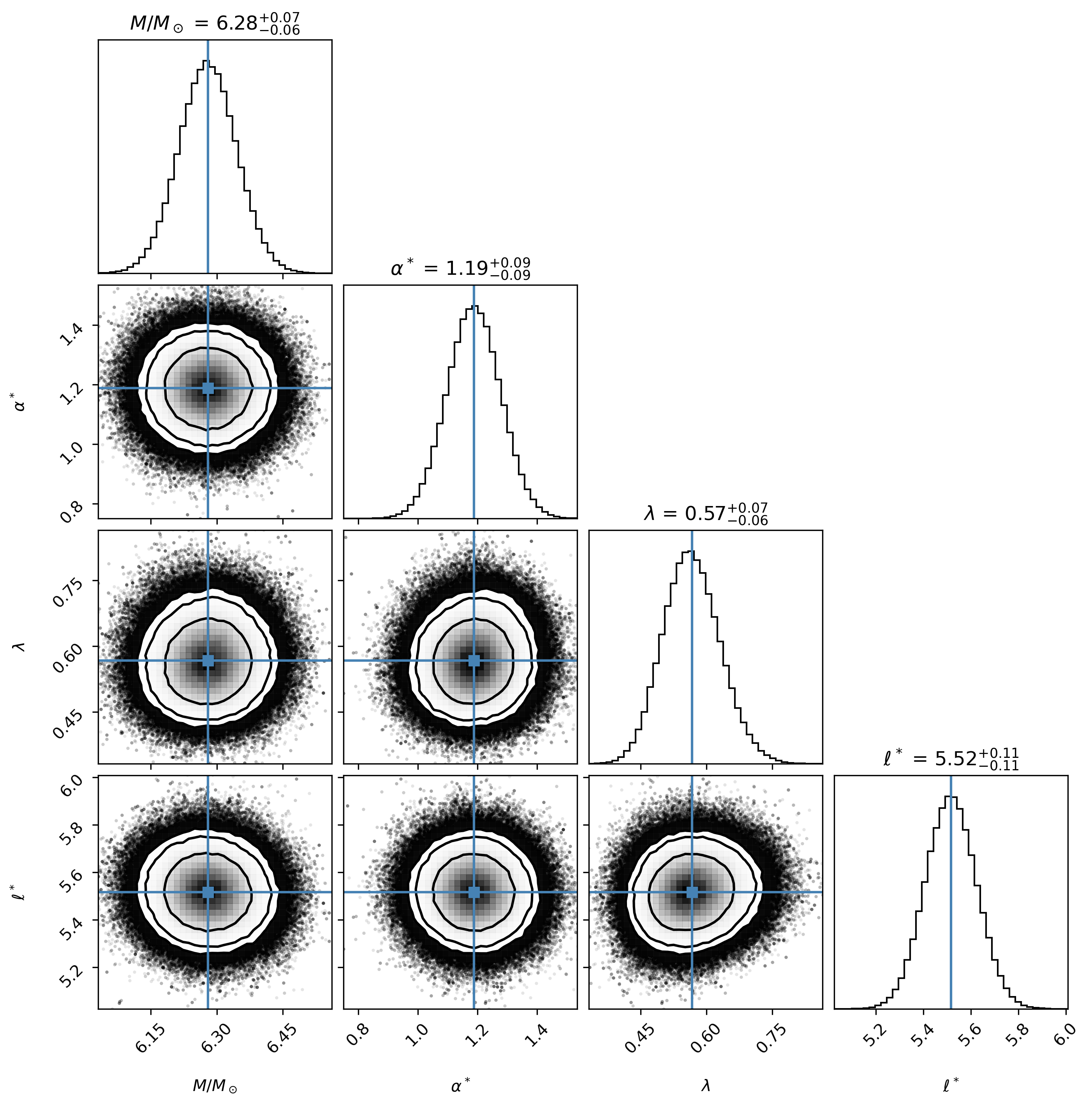
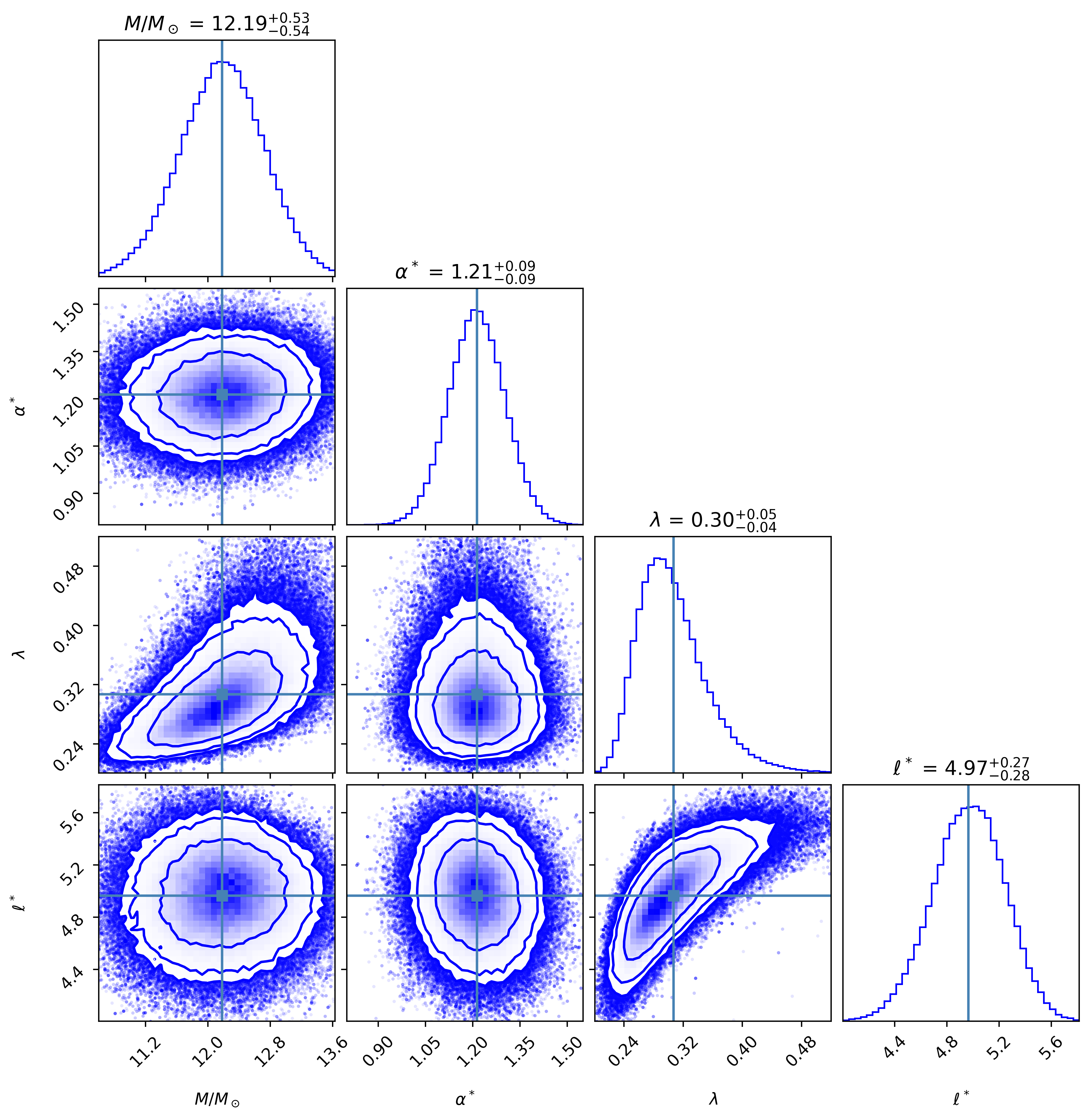
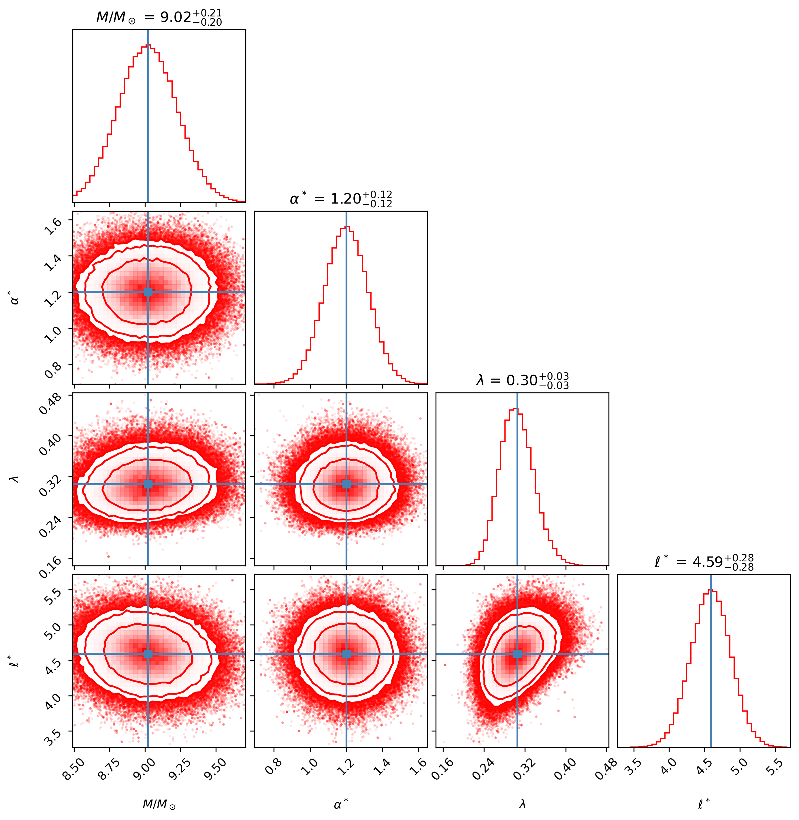
In the preceding section, we discussed the application of MCMC analysis for parameter estimation based on QPO data observed in the center of the microquasars GRO J1655-40, GRS 1915+105 & XTE J1550-564 and Milky Way galaxy given in Table 1. We have employed the MCMC code to explore the four-dimensional parameter space of the traversable wormhole solution. In this case, we have considered Sgr A* to be a supermassive wormhole candidate and studied three microquasars as stellar mass wormhole candidates. The results of the MCMC analysis are presented in Fig. 7. The contours in these figures depict shaded regions representing the confidence levels of 1 (68%), 2 (90%), and 3 (95%) for the posterior probability distributions of the complete set of parameters. The figure comprises four panels: the upper-left panel corresponds to quasar Sgr , the upper-right panel to GRO J1655-40, the lower-left to GRS 1915 +105, and the lower-right to XTE 1550-564. The details of prior values of the parameters and which correspond to having the distribution of the values of the parameters , , and are given in Table 2 and their best-fit values for these objects are shown in Table 3.
Acknowledgement
This research is supported by Grant No. FA-F-2021-510 of the Uzbekistan Agency for Innovative Development. J.R., and B.A. acknowledge the ERASMUS + ICM project for supporting their stay at the Silesian University in Opava. J.K. gratefully acknowledges support by the DFG project Ku612/18-1. P.N. gratefully acknowledges support by the Bulgarian NSF Grant KP-06-H68/7. F.A. gratefully acknowledges the support of Czech Science Foundation Grant (GAČR) No. 23-07043S and the internal grant of the Silesian University in Opava SGS/30/2023
References
- Will (2006) C. M. Will, Living Rev. Rel. 9, 3 (2006), arXiv:gr-qc/0510072 .
- Will (2018) C. M. Will, Theory and Experiment in Gravitational Physics (Cambridge University Press, 2018).
- Berti et al. (2015) E. Berti et al., Class. Quant. Grav. 32, 243001 (2015), arXiv:1501.07274 [gr-qc] .
- Akrami et al. (2021) Y. Akrami et al. (CANTATA), Modified Gravity and Cosmology: An Update by the CANTATA Network, edited by E. N. Saridakis, R. Lazkoz, V. Salzano, P. Vargas Moniz, S. Capozziello, J. Beltrán Jiménez, M. De Laurentis, and G. J. Olmo (Springer, 2021) arXiv:2105.12582 [gr-qc] .
- Abbott et al. (2017) B. P. Abbott et al. (LIGO Scientific, Virgo, Fermi GBM, INTEGRAL, IceCube, AstroSat Cadmium Zinc Telluride Imager Team, IPN, Insight-Hxmt, ANTARES, Swift, AGILE Team, 1M2H Team, Dark Energy Camera GW-EM, DES, DLT40, GRAWITA, Fermi-LAT, ATCA, ASKAP, Las Cumbres Observatory Group, OzGrav, DWF (Deeper Wider Faster Program), AST3, CAASTRO, VINROUGE, MASTER, J-GEM, GROWTH, JAGWAR, CaltechNRAO, TTU-NRAO, NuSTAR, Pan-STARRS, MAXI Team, TZAC Consortium, KU, Nordic Optical Telescope, ePESSTO, GROND, Texas Tech University, SALT Group, TOROS, BOOTES, MWA, CALET, IKI-GW Follow-up, H.E.S.S., LOFAR, LWA, HAWC, Pierre Auger, ALMA, Euro VLBI Team, Pi of Sky, Chandra Team at McGill University, DFN, ATLAS Telescopes, High Time Resolution Universe Survey, RIMAS, RATIR, SKA South Africa/MeerKAT), Astrophys. J. Lett. 848, L12 (2017), arXiv:1710.05833 [astro-ph.HE] .
- Horndeski (1974) G. W. Horndeski, Int. J. Theor. Phys. 10, 363 (1974).
- Deffayet and Steer (2013) C. Deffayet and D. A. Steer, Class. Quant. Grav. 30, 214006 (2013), arXiv:1307.2450 [hep-th] .
- Gleyzes et al. (2015a) J. Gleyzes, D. Langlois, F. Piazza, and F. Vernizzi, Phys. Rev. Lett. 114, 211101 (2015a), arXiv:1404.6495 [hep-th] .
- Langlois and Noui (2016) D. Langlois and K. Noui, JCAP 02, 034 (2016), arXiv:1510.06930 [gr-qc] .
- Crisostomi et al. (2016a) M. Crisostomi, K. Koyama, and G. Tasinato, JCAP 04, 044 (2016a), arXiv:1602.03119 [hep-th] .
- Gleyzes et al. (2015b) J. Gleyzes, D. Langlois, F. Piazza, and F. Vernizzi, JCAP 02, 018 (2015b), arXiv:1408.1952 [astro-ph.CO] .
- Crisostomi et al. (2016b) M. Crisostomi, M. Hull, K. Koyama, and G. Tasinato, JCAP 03, 038 (2016b), arXiv:1601.04658 [hep-th] .
- Gross and Sloan (1987) D. J. Gross and J. H. Sloan, Nucl. Phys. B 291, 41 (1987).
- Metsaev and Tseytlin (1987) R. R. Metsaev and A. A. Tseytlin, Nucl. Phys. B 293, 385 (1987).
- Hochberg (1990) D. Hochberg, Phys. Lett. B 251, 349 (1990).
- Fukutaka et al. (1989) H. Fukutaka, K. Tanaka, and K. Ghoroku, Phys. Lett. B 222, 191 (1989).
- Ghoroku and Soma (1992) K. Ghoroku and T. Soma, Phys. Rev. D 46, 1507 (1992).
- Lobo and Oliveira (2009) F. S. N. Lobo and M. A. Oliveira, Phys. Rev. D 80, 104012 (2009), arXiv:0909.5539 [gr-qc] .
- Kanti et al. (2011) P. Kanti, B. Kleihaus, and J. Kunz, Phys. Rev. Lett. 107, 271101 (2011), arXiv:1108.3003 [gr-qc] .
- Kanti et al. (2012) P. Kanti, B. Kleihaus, and J. Kunz, Phys. Rev. D 85, 044007 (2012), arXiv:1111.4049 [hep-th] .
- Antoniou et al. (2020) G. Antoniou, A. Bakopoulos, P. Kanti, B. Kleihaus, and J. Kunz, Phys. Rev. D 101, 024033 (2020), arXiv:1904.13091 [hep-th] .
- Ibadov et al. (2020) R. Ibadov, B. Kleihaus, J. Kunz, and S. Murodov, Phys. Rev. D 102, 064010 (2020), arXiv:2006.13008 [gr-qc] .
- Blázquez-Salcedo et al. (2018) J. L. Blázquez-Salcedo, X. Y. Chew, and J. Kunz, Phys. Rev. D 98, 044035 (2018), arXiv:1806.03282 [gr-qc] .
- Azad et al. (2023) B. Azad, J. L. Blázquez-Salcedo, X. Y. Chew, J. Kunz, and D.-h. Yeom, Phys. Rev. D 107, 084024 (2023), arXiv:2212.12601 [gr-qc] .
- González et al. (2022) P. A. González, E. Papantonopoulos, A. Rincón, and Y. Vásquez, Phys. Rev. D 106, 024050 (2022), arXiv:2205.06079 [gr-qc] .
- Churilova et al. (2021) M. S. Churilova, R. A. Konoplya, Z. Stuchlik, and A. Zhidenko, JCAP 10, 010 (2021), arXiv:2107.05977 [gr-qc] .
- Nedkova et al. (2013) P. G. Nedkova, V. K. Tinchev, and S. S. Yazadjiev, Phys. Rev. D 88, 124019 (2013), arXiv:1307.7647 [gr-qc] .
- Gyulchev et al. (2018) G. Gyulchev, P. Nedkova, V. Tinchev, and S. Yazadjiev, Eur. Phys. J. C 78, 544 (2018), arXiv:1805.11591 [gr-qc] .
- Bambi (2013) C. Bambi, Phys. Rev. D 87, 107501 (2013), arXiv:1304.5691 [gr-qc] .
- Tsukamoto et al. (2012) N. Tsukamoto, T. Harada, and K. Yajima, Phys. Rev. D 86, 104062 (2012), arXiv:1207.0047 [gr-qc] .
- Wielgus et al. (2020) M. Wielgus, J. Horak, F. Vincent, and M. Abramowicz, Phys. Rev. D 102, 084044 (2020), arXiv:2008.10130 [gr-qc] .
- Huang et al. (2023) H. Huang, J. Kunz, J. Yang, and C. Zhang, Phys. Rev. D 107, 104060 (2023), arXiv:2303.11885 [gr-qc] .
- Chakraborty and Pradhan (2017) C. Chakraborty and P. Pradhan, JCAP 03, 035 (2017), arXiv:1603.09683 [gr-qc] .
- Harko et al. (2009) T. Harko, Z. Kovacs, and F. S. N. Lobo, Phys. Rev. D 79, 064001 (2009), arXiv:0901.3926 [gr-qc] .
- Zhou et al. (2016) M. Zhou, A. Cardenas-Avendano, C. Bambi, B. Kleihaus, and J. Kunz, Phys. Rev. D 94, 024036 (2016), arXiv:1603.07448 [gr-qc] .
- Paul et al. (2020) S. Paul, R. Shaikh, P. Banerjee, and T. Sarkar, JCAP 03, 055 (2020), arXiv:1911.05525 [gr-qc] .
- Vincent et al. (2021) F. H. Vincent, M. Wielgus, M. A. Abramowicz, E. Gourgoulhon, J. P. Lasota, T. Paumard, and G. Perrin, Astron. Astrophys. 646, A37 (2021), arXiv:2002.09226 [gr-qc] .
- Gyulchev et al. (2020) G. Gyulchev, J. Kunz, P. Nedkova, T. Vetsov, and S. Yazadjiev, Eur. Phys. J. C 80, 1017 (2020), arXiv:2003.06943 [gr-qc] .
- Gyulchev et al. (2021) G. Gyulchev, P. Nedkova, T. Vetsov, and S. Yazadjiev, Eur. Phys. J. C 81, 885 (2021), arXiv:2106.14697 [gr-qc] .
- Eichhorn et al. (2023) A. Eichhorn, R. Gold, and A. Held, Astrophys. J. 950, 117 (2023), arXiv:2205.14883 [astro-ph.HE] .
- Delijski et al. (2022) V. Delijski, G. Gyulchev, P. Nedkova, and S. Yazadjiev, Phys. Rev. D 106, 104024 (2022), arXiv:2206.09455 [gr-qc] .
- Stella and Vietri (1998) L. Stella and M. Vietri, The Astrophys Jour Lett 492, L59 (1998), arXiv:astro-ph/9709085 [astro-ph] .
- Stella et al. (1999) L. Stella, M. Vietri, and S. M. Morsink, The Astrophysical Journal 524, L63 (1999), arXiv:astro-ph/9907346 [astro-ph] .
- Rayimbaev et al. (2021a) J. Rayimbaev, P. Tadjimuratov, A. Abdujabbarov, B. Ahmedov, and M. Khudoyberdieva, Galaxies 9, 75 (2021a), arXiv:2010.12863 [gr-qc] .
- Rayimbaev et al. (2021b) J. Rayimbaev, A. Abdujabbarov, and H. Wen-Biao, Phys.Rev.D 103, 104070 (2021b).
- Rayimbaev et al. (2022a) J. Rayimbaev, A. H. Bokhari, and B. Ahmedov, Classical and Quantum Gravity 39, 075021 (2022a).
- Rayimbaev et al. (2022b) J. Rayimbaev, A. Abdujabbarov, F. Abdulkhamidov, V. Khamidov, S. Djumanov, J. Toshov, and S. Inoyatov, European Physical Journal C 82, 1110 (2022b).
- Rayimbaev et al. (2022c) J. Rayimbaev, B. Ahmedov, and A. H. Bokhari, International Journal of Modern Physics D 31, 2240004-726 (2022c).
- Rayimbaev et al. (2022d) J. Rayimbaev, B. Majeed, M. Jamil, K. Jusufi, and A. Wang, Physics of the Dark Universe 35, 100930 (2022d), arXiv:2202.11509 [gr-qc] .
- Rayimbaev et al. (2023a) J. Rayimbaev, F. Abdulxamidov, S. Tojiev, A. Abdujabbarov, and F. Holmurodov, Galaxies 11, 95 (2023a).
- Murodov et al. (2023) S. Murodov, J. Rayimbaev, B. Ahmedov, and E. Karimbaev, Universe 9, 391 (2023).
- Rayimbaev et al. (2023b) J. Rayimbaev, R. C. Pantig, A. Övgün, A. Abdujabbarov, and D. Demir, Annals of Physics 454, 169335 (2023b), arXiv:2206.06599 [gr-qc] .
- Rayimbaev et al. (2023c) J. Rayimbaev, K. F. Dialektopoulos, F. Sarikulov, and A. Abdujabbarov, European Physical Journal C 83, 572 (2023c), arXiv:2307.03019 [gr-qc] .
- Qi et al. (2023) M. Qi, J. Rayimbaev, and B. Ahmedov, European Physical Journal C 83, 730 (2023).
- Deligianni et al. (2021a) E. Deligianni, J. Kunz, P. Nedkova, S. Yazadjiev, and R. Zheleva, Phys. Rev. D 104, 024048 (2021a), arXiv:2103.13504 [gr-qc] .
- Deligianni et al. (2021b) E. Deligianni, B. Kleihaus, J. Kunz, P. Nedkova, and S. Yazadjiev, Phys. Rev. D 104, 064043 (2021b), arXiv:2107.01421 [gr-qc] .
- De Falco et al. (2021) V. De Falco, M. De Laurentis, and S. Capozziello, Phys. Rev. D 104, 024053 (2021), arXiv:2106.12564 [gr-qc] .
- Stuchlík and Vrba (2021a) Z. Stuchlík and J. Vrba, Universe 7, 279 (2021a), arXiv:2108.09562 [gr-qc] .
- Stuchlík and Vrba (2021b) Z. Stuchlík and J. Vrba, Eur. Phys. J. Plus 136, 1127 (2021b), arXiv:2110.10569 [gr-qc] .
- De Falco (2023) V. De Falco, Phys. Rev. D 108, 024051 (2023), arXiv:2307.03151 [gr-qc] .
- Bakopoulos et al. (2022) A. Bakopoulos, C. Charmousis, and P. Kanti, JCAP 05, 022 (2022), arXiv:2111.09857 [gr-qc] .
- Lu and Pang (2020) H. Lu and Y. Pang, Phys. Lett. B 809, 135717 (2020), arXiv:2003.11552 [gr-qc] .
- Hennigar et al. (2020) R. A. Hennigar, D. Kubizňák, R. B. Mann, and C. Pollack, JHEP 07, 027 (2020), arXiv:2004.09472 [gr-qc] .
- Fernandes et al. (2020) P. G. S. Fernandes, P. Carrilho, T. Clifton, and D. J. Mulryne, Phys. Rev. D 102, 024025 (2020), arXiv:2004.08362 [gr-qc] .
- Clifton et al. (2020) T. Clifton, P. Carrilho, P. G. S. Fernandes, and D. J. Mulryne, Phys. Rev. D 102, 084005 (2020), arXiv:2006.15017 [gr-qc] .
- Charmousis et al. (2022) C. Charmousis, A. Lehébel, E. Smyrniotis, and N. Stergioulas, JCAP 02, 033 (2022), arXiv:2109.01149 [gr-qc] .
- Zumalacárregui and García-Bellido (2014) M. Zumalacárregui and J. García-Bellido, Phys. Rev. D 89, 064046 (2014), arXiv:1308.4685 [gr-qc] .
- Ben Achour et al. (2016a) J. Ben Achour, D. Langlois, and K. Noui, Phys. Rev. D 93, 124005 (2016a), arXiv:1602.08398 [gr-qc] .
- Ben Achour et al. (2016b) J. Ben Achour, M. Crisostomi, K. Koyama, D. Langlois, K. Noui, and G. Tasinato, JHEP 12, 100 (2016b), arXiv:1608.08135 [hep-th] .
- Bardeen et al. (1972) J. M. Bardeen, W. H. Press, and S. A. Teukolsky, The Astrophysical Journal 178, 347 (1972).
- Ingram et al. (2016) A. Ingram, M. van der Klis, M. Middleton, C. Done, D. Altamirano, L. Heil, P. Uttley, and M. Axelsson, Monthly Notices of the Royal Astronomical Society 461, 1967 (2016), arXiv:1607.02866 [astro-ph.HE] .
- Abramowicz et al. (2004) M. A. Abramowicz, W. Kluzniak, Z. Stuchlík, and G. Török, in RAGtime 4/5: Workshops on black holes and neutron stars (2004) pp. 1–23.
- Kološ et al. (2020) M. Kološ, M. Shahzadi, and Z. Stuchlík, Eur. Phys. J. C 80, 133 (2020).
- Remillard and McClintock (2006) R. A. Remillard and J. E. McClintock, Annual Review of Astronomy and Astrophysics 44, 49 (2006), arXiv:astro-ph/0606352 [astro-ph] .
- Remillard et al. (2002) R. Remillard, M. Muno, J. McClintock, and J. Orosz, in APS April Meeting Abstracts, APS Meeting Abstracts (2002) p. N17.076.
- Orosz et al. (2011) J. A. Orosz, J. F. Steiner, J. E. McClintock, M. A. P. Torres, R. A. Remillard, C. D. Bailyn, and J. M. Miller, The Astrophysical Journal 730, 75 (2011), arXiv:1101.2499 [astro-ph.SR] .
- Foreman-Mackey et al. (2013) D. Foreman-Mackey, D. W. Hogg, D. Lang, and J. Goodman, Publ. Astron. Soc. Pac. 125, 306 (2013), arXiv:1202.3665 [astro-ph.IM] .
- Liu et al. (2023) C. Liu, H. Xu, H. Siew, T. Zhu, Q. Wu, and Y. Zhao, (2023), arXiv:2305.12323 [gr-qc] .