Discretization of Total Variation in Optimization with Integrality Constraints

Abstract

We introduce discretizations of infinite-dimensional optimization problems with total variation regularization and integrality constraints on the optimization variables. We advance the discretization of the dual formulation of the total variation term with Raviart–Thomas functions which is known from literature for certain convex problems. Since we have an integrality constraint, the previous analysis from Caillaud and Chambolle [10] does not hold anymore. Even weaker $\Gamma$-convergence results do not hold anymore because the recovery sequences generally need to attain non-integer values to recover the total variation of the limit function. We solve this issue by introducing a discretization of the input functions on an embedded, finer mesh. A superlinear coupling of the mesh sizes implies an averaging on the coarser mesh of the Raviart–Thomas ansatz, which enables to recover the total variation of integer-valued limit functions with integer-valued discretized input functions. Moreover, we are able to estimate the discretized total variation of the recovery sequence by the total variation of its limit and an error depending on the mesh size ratio. For the discretized optimization problems, we additionally add a constraint that vanishes in the limit and enforces compactness of the sequence of minimizers, which yields their convergence to a minimizer of the original problem. This constraint contains a degree of freedom whose admissible range is determined. Its choice may have a strong impact on the solutions in practice as we demonstrate with an example from imaging.

Keywords: total variation; infinite-dimensional optimization with integrality restrictions; coupled discretizations; Raviart–Thomas elements

AMS subject classification: 65D18;65K10;49M25

1 Introduction

Let $\Omega\subset\mathbb{R}^{d}$, $d\in\{1,2,3\}$, be a bounded Lipschitz domain, which is a finite union of bounded intervals or axis-aligned squares or cubes. We consider discretizations of the optimization problem

$$\begin{aligned} \min_{w\in L^{1}(\Omega)}\ &F(w)+\alpha\operatorname*{TV}(w)\\ \text{s.t.}\quad&w(x)\in W\subset\mathbb{Z}\text{ for almost all (a.a.) }x\in\Omega,\end{aligned}$$ (P)

where $W\subset\mathbb{Z}$ is a finite set of integers, $\alpha>0$, $\operatorname*{TV}:L^{1}(\Omega)\to[0,\infty]$ is the total variation, and $F:L^{1}(\Omega)\to\mathbb{R}$ is continuous and bounded from below. For example, $F$ may contain a solution operator to a PDE as in [29] where a trust-region algorithm for integer optimal control problems with total variation regularization was analyzed. Hence, the results of this work can be used to discretize the function space subproblems arising in [29]. Integer optimal control problems with total variation regularization have many applications [21, 20, 19, 23]. Other problems related to (P) are investigated in the context of image denoising, deblurring [34, 12, 32, 18], and segmentation [33]. This is because the total variation allows but penalizes jumps of the input function.

One approach, in particular for $W=\{0,1\}$, to handle the total variation in combination with the integrality condition would be to use a Modica–Mortola energy functional [31] and relax the integrality condition. Then, one drives a parameter to zero that controls the non-binarity and may recover the total variation in the limit. In this case, the difficulty of the integrality is replaced by the non-convexity of the Modica–Mortola energy, however.

Therefore, the aim of this paper is to discretize (P) such that we retain the integrality condition on the input functions while being able to recover the total variation of solutions to (P). This is challenging since the underlying mesh prescribes the geometry of the discretized input functions. Many discretizations of the total variation term can already be found in literature but focus rarely on restrictions to integers, see [14] for an overview. Approaches that rely on the primal formulation of the total variation are finite-differences discretizations and variants [36, 26, 11, 1], $P1$ discretizations [6, 7], and non-conforming discretizations with Crouzeix–Raviart functions [13]. A discretization of the dual formulation by discretizing the dual fields with Raviart–Thomas functions is presented in [10]. Related approaches based on discretized dual fields are [17, 24, 15]. While a $P1$ or Crouzeix–Raviart input function ansatz does not permit the integrality condition, the other approaches allow for piecewise constant ansatz functions. However, if there are $\Gamma$-convergence results for the discretized total variation, the recovery sequences generally need to attain non-integer values to recover the total variation of the limit functions, even if the limit functions themselves are integer-valued, see the proofs of Theorem 4 in [16] and Theorem 1.2 in [10]. The latter proves an error rate for the discretized optimization problems by means of strong duality of the continuous problems which does not hold in our integer setting.

We will solve this issue by introducing two coupled discretizations with a fine mesh for the input functions that is embedded into a coarser mesh for the total variation term. A superlinear coupling of the fine mesh size to the coarser one allows to consider integer-valued and piecewise constant discretized input functions and still be able to recover the total variation of limit functions due to an averaging effect on the coarser mesh. This makes it possible to prove convergence of the discretized total variation in the sense of $\Gamma$-convergence despite the restriction to integrality. Moreover, we are able to prove an error bound for the discretized total variation of the recovery sequence with respect to the total variation of its limit.

The discretization of the considered optimization problems is accompanied with the loss of compactness of the sequence of minimizers, which is due to possible chattering enabled by the enlarged null space of the discretized total variation caused by the coupled meshes. We compensate for this lack by adding a constraint to the discretized problems that enforces compactness on the sequence of minimizers and vanishes in the limit. This constraint contains a degree of freedom whose admissible range we determine. Even though its concrete choice is irrelevant when the mesh sizes are driven to zero, it may impact on the solutions of the discretized problems in practice. Together with the approximation properties of the discretized total variation, we prove the convergence of minimizers of the discretized problems to a minimizer of the original problem. To solve the discretized problems, we will introduce an outer approximation algorithm, which we apply to an example from imaging.

Structure of the remainder: we start by introducing the discretized total variation and analyzing its approximation properties in Section 2. Section 3 is dedicated to the discretization of the considered optimization problems and the convergence of their minimizers to a minimizer of the original problem. In Section 4, we state and analyze an outer-approximation algorithm to solve the discretized problems. We present our numerical experiments and results in Section 5 and conclude in Section 6.

2 Discretized total variation

The space of functions of bounded variation $\operatorname*{BV}(\Omega)$ is the space of functions $w\in L^{1}(\Omega)$ whose total variation is finite, that is,

$$\operatorname*{TV}(w)\coloneqq\sup\left\{\int_{\Omega}w(x)\operatorname*{div}\phi(x)\mathop{}\!\mathrm{d}x\,\middle|\,\phi\in C^{1}_{c}(\Omega;\mathbb{R}^{d})\ \text{ and }\ \sup_{\mathclap{x\in\Omega}}\|\phi(x)\|\leq 1\right\}<\infty.$$

We denote the feasible set of (P) by $L^{1}_{W}(\Omega)\coloneqq\left\{w\in L^{1}(\Omega)\middle|\,w(x)\in W\text{ for a.a.\ }x\in\Omega\right\}$ and its subset of solutions with finite objective value by $\operatorname*{BV_{W}}(\Omega)\coloneqq L^{1}_{W}(\Omega)\cap\operatorname*{BV}(\Omega)$.

Lemma 2.1.

Let $\{w^{h}\}_{h>0}\subset L^{1}_{W}(\Omega)$ be given such that $w^{h}\to w$ in $L^{1}(\Omega)$ as $h\searrow 0$. Then we have that $w\in L^{1}_{W}(\Omega)$ and $w^{h}\to w$ in $L^{p}(\Omega)$ for all $1\leq p\leq\infty$.

Proof.

The first claim follows because $w^{h}\to w$ pointwise a.e. for a subsequence, cf. Lemma 2.2 in [27]. The second claim follows because

$$\|w-w^{h}\|_{L^{p}(\Omega)}^{p}\leq\|(w-w^{h})^{p-1}\|_{L^{\infty}(\Omega)}\|w-w^{h}\|_{L^{1}(\Omega)}\to 0\text{ as }h\searrow 0,$$

since $\|(w-w^{h})^{p-1}\|_{L^{\infty}(\Omega)}\leq(\max_{w_{1},w_{2}\in W}|w_{1}-w_{2}|)^{p-1}$ for all $h>0$. ∎

By the following lemma, which was proven in Theorem 1 in [25], we can replace the test function space $C_{c}^{1}(\Omega;\mathbb{R}^{d})$ for the computation of the total variation term by $H_{0}(\operatorname*{div};\Omega)$. Since $\Omega$ is a Lipschitz domain, we may define $H_{0}(\operatorname*{div};\Omega)$ by

$$H_{0}(\operatorname*{div};\Omega)\coloneqq\left\{v\in H(\operatorname*{div};\Omega)\,\middle|\,v\cdot n|_{\partial\Omega}\equiv 0\right\},$$

where $n$ denotes the outer unit normal of $\Omega$ and $H_{0}(\operatorname*{div};\Omega)=H^{1}_{0}(\Omega)$ for $d=1$.

Lemma 2.2.

For all $w\in L^{1}(\Omega)$, it holds that

$$\operatorname*{TV}(w)=\sup\left\{\int_{\Omega}w(x)\operatorname*{div}\phi(x)\mathop{}\!\mathrm{d}x\,\middle|\,\phi\in H_{0}(\operatorname*{div};\Omega)\ \text{ and }\ \|\phi\|_{L^{\infty}(\Omega;\mathbb{R}^{d})}\leq 1\right\}.$$

In order to discretize the total variation and later problem (P), we consider finite element meshes on $\Omega$ which fulfill the following assumptions.

Assumption 2.3.

 

1. $\operatorname*{TV}$ meshes: For $h>0$, we consider a partition $\mathcal{Q}_{h}$ of $\Omega$ into intervals or axis-aligned squares or cubes $Q\in\mathcal{Q}_{h}$ of height $h>0$, that is, $\Omega=\bigcup_{Q\in\mathcal{Q}_{h}}Q$.

2. Input meshes: For each $h>0$, we consider a mesh $\mathcal{Q}_{\tau_{h}}$ of $\Omega$ of intervals or axis-aligned squares or cubes $Q\in\mathcal{Q}_{\tau_{h}}$ of height $\tau_{h}\in(0,h]$ that is embedded into the $\operatorname*{TV}$ mesh. Specifically, for each $\tilde{Q}\in\mathcal{Q}_{h}$ there exists $\mathcal{Q}_{\tilde{Q}}\subset\mathcal{Q}_{\tau_{h}}$ such that $\bigcup_{Q\in\mathcal{Q}_{Q}}Q=\tilde{Q}$.

We introduce the discretized total variation in Section 2.1. We prove its approximation properties in a $\Gamma$-convergence sense below, where Section 2.2 is dedicated to the $\liminf$ inequality and Section 2.3 provides the $\limsup$ inequality and an error estimate for the discretized total variation of the recovery sequence.

2.1 Discretization of the total variation

For a mesh $\mathcal{Q}_{h}$ with $h>0$ fulfilling Assumption 2.3.1 and $w\in\operatorname*{BV}(\Omega)$, we define the following discretization of the total variation term $\operatorname*{TV}$ as in [10] by replacing the test functions for the computation of $\operatorname*{TV}$ by Raviart–Thomas functions, that is,

$$\operatorname*{TV^{h}}(w)\coloneqq\sup\left\{\int_{\Omega}w(x)\operatorname*{div}\phi(x)\mathop{}\!\mathrm{d}x\,\middle|\,\phi\in RT0_{0}^{h}\ \text{ and }\ \|\phi\|_{L^{\infty}(\Omega,\mathbb{R}^{d})}\leq 1\right\},$$

where $RT0^{h}_{0}\coloneqq\left\{\phi\in RT0^{h}\,\middle|\,(\phi\cdot n)|_{\partial\Omega}\equiv 0\right\}$ and $n$ again denotes the outer normal of $\Omega$. The space $RT0^{h}\subset H(\operatorname*{div};\Omega)$ is the lowest-order Raviart–Thomas space defined on the mesh $\mathcal{Q}_{h}$. The space $RT0^{h}$ contains piecewise linear functions $\phi$ whose normal components $\phi\cdot n_{E}$ are continuous and constant on each facet $E$ of the cells $Q\in\mathcal{Q}_{h}$ and the respective unit normal vector $n_{E}$ to $E$. Note that $RT0^{h}=P1^{h}$ in the case $d=1$, that is, Raviart–Thomas functions are continuous in the case $d=1$ in accordance with $H(\operatorname*{div};\Omega)=H^{1}(\Omega)$. We refer to [9] for a detailed definition of $RT0^{h}$.

Lemma 2.4.

Let $\phi\in RT0^{h}$ for some $h>0$ satisfy $\|\phi\|_{L^{\infty}(\Omega;\mathbb{R}^{d})}\leq 1$. Then $\|\operatorname*{div}\phi\|_{L^{\infty}(\Omega)}\leq\frac{2d}{h}$.

Proof.

We use the notations from [9]. Then for each $Q\in\mathcal{Q}_{h}$ there holds $\phi|_{Q}\in P_{1}(Q)$ (for the case $d=1$), $\phi|_{Q}\in P_{1,0}(Q)\times P_{0,1}(Q)$ (for the case $d=2$), or $\phi|_{Q}\in P_{1,0,0}(Q)\times P_{0,1,0}(Q)\times P_{0,0,1}(Q)$ (for the case $d=3$). Consider $\phi|_{\bar{Q}}$ on the element $\bar{Q}=l+[0,h]^{d}$ with $l\in\mathbb{R}^{d}$. Then $\phi|_{\bar{Q}}(x)=a+\sum_{i=1}^{d}c_{i}e^{i}x$ for $x\in\bar{Q}$ with $a,c\in\mathbb{R}^{d}$ and $e^{i}\in\mathbb{R}^{d}$, $i\in\{1,\dots,d\}$, the canonical unit vector basis. Since $\|\phi\|_{L^{\infty}(\Omega;\mathbb{R}^{d})}\leq 1$, we have for each $i\in\{1,...,d\}$ that $|a_{i}+c_{i}x_{i}|\leq 1$ for all $x_{i}\in l_{i}+[0,h]$, in particular $|a_{i}+c_{i}l_{i}+c_{i}h|\leq 1\text{ and }|a_{i}+c_{i}l_{i}|\leq 1.$ This yields

$$|\operatorname*{div}\phi|_{\bar{Q}}|\leq\sum_{i=1}^{d}|c_{i}|\leq\sum_{i=1}^{d}\frac{1}{h}(|a_{i}+c_{i}l_{i}+c_{i}h|+|a_{i}+c_{i}l_{i}|)\leq\sum_{i=1}^{d}\frac{2}{h}=\frac{2d}{h}.$$

∎

In contrast to $\operatorname*{TV}$, the discretized total variation $\operatorname*{TV^{h}}$ always admits a maximizer and is thus always finite. Moreover, $\operatorname*{TV}$ is always an upper bound for $\operatorname*{TV^{h}}$.

Lemma 2.5.

Let $w\in L^{1}_{W}(\Omega)$. Then there is some $\phi\in RT0^{h}_{0}$ with $\|\phi\|_{L^{\infty}(\Omega;\mathbb{R}^{d})}\leq 1$ such that $\operatorname*{TV^{h}}(w)=\int_{\Omega}w(x)\operatorname*{div}\phi(x)\mathop{}\!\mathrm{d}x<\infty$ and $\operatorname*{TV^{h}}(w)\leq\operatorname*{TV}(w)$.

Proof.

$\operatorname*{TV^{h}}(w)\leq\operatorname*{TV}(w)$ follows from Lemma 2.2 since $RT0_{0}^{h}\subset H_{0}(\operatorname*{div};\Omega)$. The existence of a maximizer of $\operatorname*{TV^{h}}$ follows from the fact that the corresponding maximization problem can be rewritten as a finite-dimensional optimization problem with linear objective function and compact feasible set. This is because $RT0_{0}^{h}$ is finite-dimensional, $\operatorname*{div}\phi$ for $\phi\in RT0_{0}^{h}$ is constant on the grid cells $Q\in\mathcal{Q}_{h}$, and the feasible set of $\operatorname*{TV^{h}}(w)$ can be described by finitely many convex inequalities by bounding the Euclidean norm of the point evaluations of $\phi$ in each node of the mesh $\mathcal{Q}_{h}$ by $1$. ∎

In order to discretize (P), we replace the total variation term $\operatorname*{TV}(w)$ by the discretized total variation term $\operatorname*{TV^{h}}(w)$ in the objective. As a result, we can no longer guarantee the existence of minimizers, as stated in the following remark, because $\operatorname*{TV^{h}}$ has a greater null space than $\operatorname*{TV}$. We will fix this issue in Section 3.

Remark 2.6.

If we replace $\operatorname*{TV}$ by $\operatorname*{TV^{h}}$ in problem (P), we can not guarantee the existence of minimizers anymore because $\operatorname*{TV^{h}}$ has a greater null space than $\operatorname*{TV}$. This is due to the fact that for each $w\in L^{1}(\Omega)$, we have that

$$\int_{\Omega}w(x)\operatorname*{div}\phi(x)\mathop{}\!\mathrm{d}x=\sum_{Q\in\mathcal{Q}_{h}}d_{Q}\int_{Q}w(x)\mathop{}\!\mathrm{d}x=\int_{\Omega}\tilde{w}(x)\operatorname*{div}\phi(x)\mathop{}\!\mathrm{d}x$$ (1)

for all $\phi\in RT0^{h}$ with $\operatorname*{div}\phi|_{Q}\eqqcolon d_{Q}\in\mathbb{R}$ for all $Q\in\mathcal{Q}_{h}$ and all $\tilde{w}\in L^{1}(\Omega)$ with $\int_{Q}\tilde{w}(x)\mathop{}\!\mathrm{d}x=\int_{Q}w(x)\mathop{}\!\mathrm{d}x$ for all $Q\in\mathcal{Q}_{h}$. This in particular yields $\operatorname*{TV^{h}}(w)=\operatorname*{TV^{h}}(\tilde{w})$. Hence, there may exist a minimizing sequence $\{w^{n}\}_{n\in\mathbb{N}}\subset\operatorname*{BV_{W}}(\Omega)$ consisting of chattering functions (for example with checkerboard structure) with $\operatorname*{TV^{h}}(w^{n})=0$ for all $n\in\mathbb{N}$ that converges weakly to some limit function that is not in $\operatorname*{BV_{W}}(\Omega)$.

2.2 Lim inf inequality for $\operatorname*{TV^{h}}$

Let a mesh $\mathcal{Q}_{\tau}$ with $\tau>0$ fulfill Assumption 2.3. We define the space of functions that are piecewise constant on the mesh cells $Q\in\mathcal{Q}_{\tau}$ by $P0^{\tau}$. Let $\Pi_{P0^{\tau}}:L^{1}(\Omega)\to P0^{\tau}$ denote the projection onto $P0^{\tau}$.

Lemma 2.7.

Let $w\in L^{1}_{W}(\Omega)$. Then $\|w-\Pi_{P0^{\tau}}w\|_{L^{1}(\Omega)}\to 0\text{ as }\tau\searrow 0$. Moreover, for all $w\in\operatorname*{BV_{W}}(\Omega)$ there holds $\|w-\Pi_{P0^{\tau}}w\|_{L^{1}(\Omega)}\leq\sqrt{d}\tau\operatorname*{TV}(w)$.

Proof.

Let $w\in L^{1}_{W}(\Omega)$. Lebesgue’s differentiation theorem [35, Chap. 3, Cor. 1.6 and 1.7] gives $\Pi_{P0^{\tau}}w\to w$ pointwise a.e. in $\Omega$ as $\tau\searrow 0$. Moreover, $\|\Pi_{P0^{\tau}}w\|_{L^{\infty}(\Omega)}\leq\max_{w\in W}|w|\in\mathbb{R}$ such that Lebesgue’s dominated convergence theorem yields $\|w-\Pi_{P0^{\tau}}w\|_{L^{1}(\Omega)}\to 0$ as $\tau\searrow 0$. Since $\Omega$ is in particular of finite perimeter, the proof of the second claim runs along the lines of Theorem 12.26, particularly (12.24), in [28]. A similar proof for $\Omega=(0,1)^{2}$ is given in Lemma 3.2 in [10]. ∎

The following estimate

$$\|\phi-I_{RT0^{h}}\phi\|_{L^{\infty}(\Omega;\mathbb{R}^{d})}\leq\sup_{Q\in\mathcal{Q}_{h}}(1+\sqrt{d})\|c_{Q}-\phi\|_{L^{\infty}(Q;\mathbb{R}^{d})}\leq hC(\phi)$$ (2)

holds for all $\phi\in C_{c}^{1}(\Omega;\mathbb{R}^{d})$, where $I_{RT0^{h}}:C^{1}_{c}(\Omega;\mathbb{R}^{d})\to RT0^{h}$ denotes the interpolation operator for $RT0^{h}$ as defined in § III.3.3 in [9], $c_{Q}\coloneqq\frac{1}{|Q|}\int_{Q}\phi(x)\mathop{}\!\mathrm{d}x\in\mathbb{R}^{d}$, and $C(\phi)\coloneqq(d+\sqrt{d})\sqrt{\sum_{i=1}^{d}\|\nabla\phi_{i}\|_{L^{\infty}(\Omega;\mathbb{R}^{d})}^{2}}>0$. Similar results are proven for tetrahedral meshes in Theorem 6.3 in [2] and for the projection onto $RT0^{h}$ in the two-dimensional case in Lemma 3.6 in [10].

Lemma 2.8.

Let $\{w^{h}\}_{h>0}\subset L^{1}(\Omega)$ with $w^{h}\to w$ in $L^{1}(\Omega)$ and $w\in L^{2}(\Omega)$. Let $\phi\in C^{1}_{c}(\Omega;\mathbb{R}^{d})$ satisfy $\|\phi\|_{L^{\infty}(\Omega;\mathbb{R}^{d})}\leq 1$. Then

$$\int_{\Omega}\operatorname*{div}\phi(x)w(x)\mathop{}\!\mathrm{d}x\leq\liminf_{h\searrow 0}\operatorname*{TV^{h}}(w^{h}).$$ (3)

Proof.

Let $\varepsilon>0$. Then we approximate $\phi$ with $\hat{\phi}\coloneqq(1-\varepsilon)\phi\in C_{c}^{1}(\Omega;\mathbb{R}^{d})$ such that $\|\hat{\phi}\|_{L^{\infty}(\Omega;\mathbb{R}^{d})}=(1-\varepsilon)\|\phi\|_{L^{\infty}(\Omega;\mathbb{R}^{d})}\leq 1-\varepsilon$ and

$$\int_{\Omega}\operatorname*{div}\phi(x)w(x)\mathop{}\!\mathrm{d}x =\int_{\Omega}\operatorname*{div}\hat{\phi}(x)w(x)\mathop{}\!\mathrm{d}x+\varepsilon\int_{\Omega}\operatorname*{div}\phi(x)w(x)\mathop{}\!\mathrm{d}x$$

$$\leq\int_{\Omega}\operatorname*{div}\hat{\phi}(x)w(x)\mathop{}\!\mathrm{d}x+\underbrace{\|\operatorname*{div}\phi\|_{L^{\infty}(\Omega)}\|w\|_{L^{1}(\Omega)}}_{c_{1}\coloneqq}\varepsilon.$$

By virtue of the error estimate (2), we obtain that $\|I_{RT0^{h}}\hat{\phi}\|_{L^{\infty}(\Omega;\mathbb{R}^{d})}\leq 1$ holds for all $h\leq\frac{\varepsilon}{C(\hat{\phi})}$ for some constant $C(\hat{\phi})>0$. Moreover, since $\hat{\phi}$ has compact support in $\Omega$, there holds $\hat{\phi}\cdot n\equiv 0$ on $\partial\Omega$, where $n$ denotes the unit outer normal of $\Omega$, so that $I_{RT0^{h}}\hat{\phi}\in RT0^{h}_{0}$. Since $\hat{\phi}\in C^{1}_{c}(\Omega;\mathbb{R}^{d})$, there exists a constant $M(\hat{\phi})>0$ only depending on $\hat{\phi}$ such that $\|\operatorname*{div}\hat{\phi}\|_{L^{\infty}(\Omega)}\leq M(\hat{\phi})$. This implies that $\|\Pi_{P0^{h}}\operatorname*{div}\hat{\phi}\|_{L^{\infty}(\Omega)}\leq M(\hat{\phi})$ for all $h>0$ such that

$$\int_{\Omega}\operatorname*{div}I_{RT0^{h}}\hat{\phi}(x)w(x)\mathop{}\!\mathrm{d}x$$

$$\leq\int_{\Omega}\operatorname*{div}I_{RT0^{h}}\hat{\phi}(x)w^{h}(x)\mathop{}\!\mathrm{d}x+\|\operatorname*{div}I_{RT0^{h}}\hat{\phi}\|_{L^{\infty}(\Omega)}\|w^{h}-w\|_{L^{1}(\Omega)}$$

$$\leq\operatorname*{TV^{h}}(w^{h})+\|\operatorname*{div}I_{RT0^{h}}\hat{\phi}\|_{L^{\infty}(\Omega)}\|w^{h}-w\|_{L^{1}(\Omega)}$$

$$=\operatorname*{TV^{h}}(w^{h})+\|\Pi_{P0^{h}}\operatorname*{div}\hat{\phi}\|_{L^{\infty}(\Omega)}\|w^{h}-w\|_{L^{1}(\Omega)}$$

$$\leq\operatorname*{TV^{h}}(w^{h})+M(\hat{\phi})\|w^{h}-w\|_{L^{1}(\Omega)},$$

where we used $\operatorname*{div}I_{RT0^{h}}\hat{\phi}=\Pi_{P0^{h}}\operatorname*{div}\hat{\phi}$ from Proposition 3.7 in § III.3 in [9], yielding

$$\int_{\Omega}\operatorname*{div}\phi(x)w(x)\mathop{}\!\mathrm{d}x\leq\int_{\Omega}\operatorname*{div}\hat{\phi}(x)w(x)\mathop{}\!\mathrm{d}x+c_{1}\varepsilon$$

$$=\int_{\Omega}\operatorname*{div}I_{RT0^{h}}\hat{\phi}(x)w(x)\mathop{}\!\mathrm{d}x+\int_{\Omega}\operatorname*{div}(\hat{\phi}-I_{RT0^{h}}\hat{\phi})(x)w(x)\mathop{}\!\mathrm{d}x+c_{1}\varepsilon$$

$$\leq\operatorname*{TV^{h}}(w^{h})+M(\hat{\phi})\|w^{h}-w\|_{L^{1}(\Omega)}+\|\operatorname*{div}(\hat{\phi}-I_{RT0^{h}}\hat{\phi})\|_{L^{2}(\Omega)}\|w\|_{L^{2}(\Omega)}+c_{1}\varepsilon.$$

By Proposition 3.8 in § III.3 in [9], there holds $\|\operatorname*{div}(\hat{\phi}-I_{RT0^{h}}\hat{\phi})\|_{L^{2}(\Omega)}\to 0$ as $h\searrow 0$. Since $w\in L^{2}(\Omega)$, driving $h\searrow 0$ implies that

$$\int_{\Omega}\operatorname*{div}\phi(x)w(x)\mathop{}\!\mathrm{d}x\leq c_{1}\varepsilon+\liminf_{h\searrow 0}\operatorname*{TV^{h}}(w^{h}).$$

The claim follows because $\varepsilon>0$ was chosen arbitrarily. ∎

Theorem 2.9.

Let $\{w^{h}\}_{h>0}\subset L^{1}(\Omega)$ with $w^{h}\to w$ in $L^{1}(\Omega)$ as $h\searrow 0$ and $w\in L^{2}(\Omega)$. Then

$$\operatorname*{TV}(w)\leq\liminf_{h\searrow 0}\operatorname*{TV^{h}}(w^{h}).$$

Proof.

We supremize over all $\phi\in C_{c}^{1}(\Omega;\mathbb{R}^{d})$ with $\|\phi\|_{L^{\infty}(\Omega;\mathbb{R}^{d})}\leq 1$ in (3). ∎

Up to this point the discretization of the input function $w$ has not been relevant. Indeed, the previous statements hold for arbitrary sequences with $w^{h}\to w$ in $L^{1}(\Omega)$ with $w\in L^{2}(\Omega)$. Instead, the discretized total variation $\operatorname*{TV^{h}}$ discretizes its inputs $w$ implicitly in the sense that $\operatorname*{TV^{h}}(w)=\operatorname*{TV^{h}}(\Pi_{P0^{h}}w)$, see (1). That means if we would waive the integrality constraint for the discretized problems, we could approximate the total variation of a given function $w\in\operatorname*{BV_{W}}(\Omega)$ with the discretized total variation of the projections $\Pi_{P0^{h}}w$. In particular, we refer to the results in [10]. Since we additionally—and in particular differing from [10]—require that the discretized input functions only attain values in the discrete set $W$, we can not work with the projections $\Pi_{P0^{h}}w$ as in [10]. Due to the given geometry of the mesh, it is generally not possible to approximate the term $\operatorname*{TV}(w)$ for $w\in\operatorname*{BV_{W}}(\Omega)$ with $\operatorname*{TV^{h}}$ of functions in $P0^{h}\cap\operatorname*{BV_{W}}(\Omega)$, as the following example shows.

Figure 1: Example for the construction in Example 2.10 with $k=1$. The level sets of the limit function $w$ are separated by the solid line and the level sets of the rounding of $\Pi_{P0^{h}}w$ are separated by the dotted line. Nonzero fluxes of $\phi$ are indicated next to the corresponding edges of the grid cells.

Example 2.10.

Consider $\Omega=(0,1)\times(0,0.4)$ and the mesh $\mathcal{Q}_{h}$ consisting of squares of size $h=\frac{1}{15k}$ for $k\in\mathbb{N}$. Define $w=\chi_{\{(\frac{1}{3},-1)^{T}x\geq 0\}}$ and consider $w^{h}\in P0^{h}\cap\operatorname*{BV_{W}}(\Omega)$ obtained by rounding the projection $\Pi_{P0^{h}}w$ on each square to the nearest value in $W$, see Fig. 1 for an example for $k=1$. Let $\phi\in RT0^{h}$ be the Raviart–Thomas function that is defined by the fluxes over the edges of the grid cells as exemplarily illustrated in Fig. 1. It is immediate that $\|\phi\|_{L^{\infty}(\Omega;\mathbb{R}^{d})}\leq 1$. Denote by $\mathcal{E}_{h}$ the interior edges of the mesh $\mathcal{Q}_{h}$ and let $n_{E}$ be a unit normal vector to an edge $E\in\mathcal{E}_{h}$. Let $w^{h}_{E^{+}}$ and $w^{h}_{E^{-}}$ denote the values of $w^{h}$ on the two cubes adjoining $E$. Then,

$$\operatorname*{TV^{h}}(w^{h}) \geq\int_{\Omega}\operatorname*{div}\phi\,w^{h}\mathop{}\!\mathrm{d}x=\sum_{E\in\mathcal{E}_{h}}|w^{h}_{E^{+}}-w^{h}_{E^{-}}|\,\int_{E}\phi\cdot n_{E}\mathop{}\!\mathrm{d}\mathcal{H}^{1}(x)$$

$$=\frac{1}{15k}\left(\left(5k-1\right)\left(1+2\cdot\frac{2}{\sqrt{5}}+\frac{1}{\sqrt{5}}\right)+2\cdot\frac{1}{\sqrt{2}}\right)$$

$$=\frac{1+\sqrt{5}}{3}+\frac{\sqrt{2}-1-\sqrt{5}}{15k}\to\frac{1+\sqrt{5}}{3}\approx 1.078\quad\text{as }k\to\infty.$$

On the other hand, $\operatorname*{TV}(w)=\frac{\sqrt{10}}{3}\approx 1.054$ such that $\operatorname*{TV^{h}}(w^{h})\not\to\operatorname*{TV}(w)$ as $h\searrow 0$. Instead, there holds $\operatorname*{TV^{h}}(w^{h})>\operatorname*{TV}(w)$ for $k\geq 5$.

2.3 Lim sup inequality for $\operatorname*{TV^{h}}$

To achieve an averaging effect by other means than the projection $\Pi_{P0^{h}}$, we discretize the functions $w\in\operatorname*{BV_{W}}(\Omega)$ on a finer mesh $\mathcal{Q}_{\tau_{h}}$ embedded into the mesh $\mathcal{Q}_{h}$ for $\operatorname*{TV^{h}}$ such that Assumption 2.3 is fulfilled. This allows to recover $\operatorname*{TV}(w)$ with $\operatorname*{TV^{h}}(w^{\tau_{h}})$ with functions $w^{\tau_{h}}\in P0^{\tau_{h}}\cap\operatorname*{BV_{W}}(\Omega)$ when the mesh sizes are superlinearly coupled, that is, $\frac{\tau_{h}}{h}\searrow 0$ as $h\searrow 0$.

Definition 2.11.

We define the operator $R_{P0^{\tau}}^{W}:\operatorname*{BV_{W}}(\Omega)\to\operatorname*{BV_{W}}(\Omega)\cap P0^{\tau}$ for $\tau>0$ and a corresponding mesh $\mathcal{Q}_{\tau}$ as follows. For $w\in\operatorname*{BV_{W}}(\Omega)$ and $Q\in\mathcal{Q}_{\tau}$, let

$$R_{P0^{\tau}}^{W}(v)|_{Q}\in\operatorname*{arg\,min}\left\{\left|\frac{1}{|Q|}\int_{Q}w(x)\mathop{}\!\mathrm{d}x-\omega\right|\,\middle|\,\omega\in W\text{ and }\left|w|_{Q}^{-1}(\omega)\right|>0\right\}.$$

If the minimizer is not unique, we choose the smallest one.

Similar to Lemma 2.7, we obtain convergence results for the sequence $\{R_{P0^{\tau}}^{W}(w)\}_{\tau>0}$ for $\tau\searrow 0$ with a convergence rate depending on $\operatorname*{TV}(w)$ if $w\in\operatorname*{BV_{W}}(\Omega)$.

Lemma 2.12.

Let $w\in L^{1}_{W}(\Omega)$. Then

$$\|w-R^{W}_{P0^{\tau}}(w)\|_{L^{1}(\Omega)}\leq 2\|w-\Pi_{P0^{\tau}}w\|_{L^{1}(\Omega)}\to 0\text{ as }\tau\searrow 0.$$

Moreover, for all $w\in\operatorname*{BV_{W}}(\Omega)$ the following estimates hold:

$$\|w-R^{W}_{P0^{\tau}}(w)\|_{L^{1}(\Omega)}\leq 2\sqrt{d}\tau\operatorname*{TV}(w)\>\text{ and }\>\|R^{W}_{P0^{\tau}}(w)-\Pi_{P0^{\tau}}w\|_{L^{1}(\Omega)}\leq\sqrt{d}\tau\operatorname*{TV}(w).$$

Proof.

For the first claim, let $w\in L^{1}_{W}(\Omega)$. By Definition 2.11, there holds $\|\Pi_{P0^{\tau}}w-R^{W}_{P0^{\tau}}(w)\|_{L^{1}(\Omega)}\leq\|w-\Pi_{P0^{\tau}}w\|_{L^{1}(\Omega)}$ due to $|(\Pi_{P0^{\tau}}w)(x)-(R^{W}_{P0^{\tau}}(w))(x)|$ $\leq|(\Pi_{P0^{\tau}}w)(x)-w(x)|$ for a.a. $x\in\Omega$. Hence,

$$\|w-R^{W}_{P0^{\tau}}(w)\|_{L^{1}(\Omega)} \leq\|w-\Pi_{P0^{\tau}}w\|_{L^{1}(\Omega)}+\|\Pi_{P0^{\tau}}w-R^{W}_{P0^{\tau}}(w)\|_{L^{1}(\Omega)}$$

$$\leq 2\|w-\Pi_{P0^{\tau}}w\|_{L^{1}(\Omega)}\to 0\text{ as }\tau\searrow 0.$$

The second claim follows then by Lemma 2.7. ∎

With these preparations, we are now able to prove a result corresponding to Lemma 3.1 in [10], where it is stated that $\operatorname*{TV^{h}}(\Pi_{P0^{h}}w)\leq\operatorname*{TV}(w)$ for $w\in L^{1}(\Omega)$.

Proposition 2.13.

Let $w\in\operatorname*{BV_{W}}(\Omega)$ and a tuple $(h,\tau_{h})$ with $h>0$ be given such that Assumption 2.3 is fulfilled. Then

$$\operatorname*{TV^{h}}(R^{W}_{P0^{\tau_{h}}}(w))\leq\operatorname*{TV^{h}}(w)+\varepsilon(\tau_{h},h,w)\leq\operatorname*{TV}(w)+\varepsilon(\tau_{h},h,w)$$ (4)

with $\varepsilon(\tau_{h},h,w)\coloneqq\sqrt{d}\operatorname*{TV}(w)\frac{2d\tau_{h}}{h}$.

Proof.

Let $w\in\operatorname*{BV_{W}}(\Omega)$. We define $w^{\tau_{h}}\coloneqq R^{W}_{P0^{\tau_{h}}}(w)\in\operatorname*{BV_{W}}(\Omega)$ and $\bar{w}^{\tau_{h}}\coloneqq\Pi_{P0^{\tau_{h}}}w\in\operatorname*{BV}(\Omega)$. Let $\phi\in RT0_{0}^{h}$ with $\|\phi\|_{L^{\infty}(\Omega;\mathbb{R}^{d})}\leq 1$. Then

$$\int_{\Omega}w^{\tau_{h}}(x)\operatorname*{div}\phi(x)\mathop{}\!\mathrm{d}x =\int_{\Omega}\bar{w}^{\tau_{h}}(x)\operatorname*{div}\phi(x)\mathop{}\!\mathrm{d}x+\int_{\Omega}(w^{\tau_{h}}(x)-\bar{w}^{\tau_{h}}(x))\operatorname*{div}\phi(x)\mathop{}\!\mathrm{d}x$$

$$\leq\operatorname*{TV^{h}}(w)+\|w^{\tau_{h}}-\bar{w}^{\tau_{h}}\|_{L^{1}(\Omega)}\|\operatorname*{div}\phi\|_{L^{\infty}(\Omega)},$$

where we have used that the meshes $\mathcal{Q}_{h}$ and $\mathcal{Q}_{\tau_{h}}$ fulfill Assumption 2.3 and that $\operatorname*{div}\phi$ is constant on each $Q\in\mathcal{Q}_{h}$ to deduce the inequality. By Lemma 2.4, it follows that $\|\operatorname*{div}\phi\|_{L^{\infty}(\Omega)}\leq\frac{2d}{h}$, and Lemma 2.12 yields $\|w^{\tau_{h}}-\bar{w}^{\tau_{h}}\|_{L^{1}(\Omega)}\leq\sqrt{d}\tau_{h}\operatorname*{TV}(w)$ which implies $\int_{\Omega}w^{\tau_{h}}(x)\operatorname*{div}\phi(x)\mathop{}\!\mathrm{d}x\leq\operatorname*{TV^{h}}(w)+\varepsilon(\tau_{h},h,w)$. ∎

We are now able to prove the $\limsup$ inequality for $\operatorname*{TV^{h}}$.

Theorem 2.14.

Let $w\in L^{1}_{W}(\Omega)$ and tuples $\{(h,\tau_{h})\}_{h>0}$ be given such that Assumption 2.3 is fulfilled and $\frac{\tau_{h}}{h}\searrow 0$ as $h\searrow 0$. Then there holds

$$\operatorname*{TV}(w)\geq\limsup_{h\searrow 0}\operatorname*{TV^{h}}(R^{W}_{P0^{\tau_{h}}}(w)).$$

Proof.

The claim follows from Proposition 2.13 by applying $\limsup_{h\searrow 0}$ to both sides of (4) and using the assumption $\frac{\tau_{h}}{h}\searrow 0$. ∎

The embedding of the meshes $\mathcal{Q}_{\tau_{h}}$ into the $\mathcal{Q}_{h}$ and the superlinear coupling of their mesh sizes yield a lower bound estimate for the discretized total variation of the recovery sequence from Theorem 2.14 using techniques from Proposition 3.7 in [10].

Proposition 2.15.

Let $w\in\operatorname*{BV_{W}}(\Omega)$, $\operatorname*{TV}(w)=-\int_{\Omega}\operatorname*{div}\phi(x)w(x)\mathop{}\!\mathrm{d}x$ with $\phi\in C^{1}_{c}(\Omega;\mathbb{R}^{d})$, and $\{(h,\tau_{h})\}_{h>0}$ be coupled such that Assumption 2.3 is fulfilled. Then

$$\operatorname*{TV^{h}}(R^{W}_{P0^{\tau_{h}}}(w))\geq\operatorname*{TV}(w)-c(w,\phi)\left(h^{2}+h+\tau_{h}+\frac{\tau_{h}}{h}\right)$$

holds with some constant $c(w,\phi)>0$, depending on $w$ and $\phi$.

Proof.

Let $\phi^{h}\coloneqq I_{RT0^{h}}\phi\in RT0^{h}_{0}$ for $h>0$. By (2), there holds $\|\phi^{h}\|_{L^{\infty}(\Omega)}\leq 1+Ch$ with $C=C(\phi)>0$. We define $\tilde{\phi}^{h}\coloneqq\frac{1}{1+Ch}\phi^{h}\in RT0^{h}_{0}$ for $h>0$, which fulfills $\|\tilde{\phi}^{h}\|_{L^{\infty}(\Omega)}\leq 1$. Moreover, we define $w^{h}=\Pi_{P0^{h}}w$ for $h>0$, which fulfills $\int_{\Omega}w(x)w^{h}(x)\mathop{}\!\mathrm{d}x=\|w^{h}\|_{L^{2}(\Omega)}^{2}$ due to the optimality condition of the projection. By Proposition 3.7 in § III.3 in [9], there holds $\operatorname*{div}I_{RT0^{h}}\phi=\Pi_{P0^{h}}\operatorname*{div}\phi$ so that also $\int_{\Omega}\operatorname*{div}\phi(x)\operatorname*{div}\phi^{h}(x)\mathop{}\!\mathrm{d}x=\|\operatorname*{div}\phi^{h}\|_{L^{2}(\Omega)}^{2}$. Hence, there holds

$$\operatorname*{TV}(w)=-\frac{1}{2}\|\operatorname*{div}\phi+w\|_{L^{2}(\Omega)}^{2}+\frac{1}{2}\|w\|_{L^{2}(\Omega)}^{2}+\frac{1}{2}\|\operatorname*{div}\phi\|_{L^{2}(\Omega)}^{2}$$

$$\leq-\frac{1}{2}\|\operatorname*{div}\phi^{h}+w^{h}\|_{L^{2}(\Omega)}^{2}+\frac{1}{2}\|w\|_{L^{2}(\Omega)}^{2}+\frac{1}{2}\|\operatorname*{div}\phi\|_{L^{2}(\Omega)}^{2}$$

$$=\frac{1}{2}\big{(}\|\operatorname*{div}\phi\|_{L^{2}(\Omega)}^{2}-\|\operatorname*{div}\phi^{h}\|_{L^{2}(\Omega)}^{2}+\|w\|_{L^{2}(\Omega)}^{2}-\|w^{h}\|_{L^{2}(\Omega)}^{2}\big{)}-\int_{\Omega}\operatorname*{div}\phi^{h}(x)w^{h}(x)\mathop{}\!\mathrm{d}x$$

$$=\frac{1}{2}\|\operatorname*{div}(\phi^{h}-\phi)\|_{L^{2}(\Omega)}^{2}+\frac{1}{2}\|w-w^{h}\|_{L^{2}(\Omega)}^{2}-(1+Ch)\int_{\Omega}\operatorname*{div}\tilde{\phi}^{h}(x)w^{h}(x)\mathop{}\!\mathrm{d}x$$

$$\leq b^{2}h^{2}\|\operatorname*{div}\phi\|_{L^{2}(\Omega)}^{2}+\frac{1}{2}\|w-w^{h}\|_{L^{1}(\Omega)}\|w-w^{h}\|_{L^{\infty}(\Omega)}+(1+Ch)\operatorname*{TV^{h}}(w^{h}),$$

with $\|\operatorname*{div}(\phi^{h}-\phi)\|_{L^{2}(\Omega)}\leq b\|\operatorname*{div}\phi\|_{L^{2}(\Omega)}$ for a constant $b>0$ by Proposition 3.8 in § III.3 in [9]. Lemma 2.7 gives $\|w-w^{h}\|_{L^{1}(\Omega)}\leq\sqrt{d}\tau_{h}\operatorname*{TV}(w)$. Since $w,w^{h}\in\operatorname*{BV_{W}}(\Omega)$, there holds $\|w-w^{h}\|_{L^{\infty}}\leq\max_{w_{1},w_{2}\in W}|w_{1}-w_{2}|\eqqcolon W_{\max}$. There holds $\operatorname*{TV^{h}}(w^{h})=\operatorname*{TV^{h}}(\Pi_{P0^{\tau_{h}}}w)$ due to $\int_{Q}w^{h}(x)\mathop{}\!\mathrm{d}x=\int_{Q}\Pi_{P0^{\tau_{h}}}w(x)\mathop{}\!\mathrm{d}x$ for all $Q\in\mathcal{Q}_{h}$ by Assumption 2.3. By Lemma 2.5, there exists $\hat{\phi}^{h}\in RT0^{h}_{0}$ with $\|\hat{\phi}^{h}\|_{L^{\infty}(\Omega)}\leq 1$ so that

$$\operatorname*{TV^{h}}(\Pi_{P0^{\tau_{h}}}w) \hskip 28.45274pt=\int_{\Omega}\operatorname*{div}\hat{\phi}^{h}(x)\Pi_{P0^{\tau_{h}}}w(x)\mathop{}\!\mathrm{d}x$$

$$=\int_{\Omega}\operatorname*{div}\hat{\phi}^{h}(x)(\Pi_{P0^{\tau_{h}}}w(x)-R^{W}_{P0^{\tau_{h}}}(w)(x))\mathop{}\!\mathrm{d}x+\int_{\Omega}\operatorname*{div}\hat{\phi}^{h}(x)R^{W}_{P0^{\tau_{h}}}(w)(x)\mathop{}\!\mathrm{d}x$$

$$\leq\|\operatorname*{div}\hat{\phi}^{h}\|_{L^{\infty}(\Omega)}\|\Pi_{P0^{\tau_{h}}}w-R^{W}_{P0^{\tau_{h}}}(w)\|_{L^{1}(\Omega)}+\operatorname*{TV^{h}}(R^{W}_{P0^{\tau_{h}}}(w))$$

$$\leq\frac{4d\sqrt{d}\tau_{h}}{h}\operatorname*{TV}(w)+\operatorname*{TV^{h}}(R^{W}_{P0^{\tau_{h}}}(w)),$$

where the last inequality follows from Lemmas 2.4 and 2.12. In total, we obtain

$$\operatorname*{TV^{h}}(R^{W}_{P0^{\tau_{h}}}(w))-\operatorname*{TV}(w)\\ \geq-\frac{\left(Ch+\frac{1}{2}W_{\max}\sqrt{d}\tau_{h}+(1+Ch)\frac{4d\sqrt{d}\tau_{h}}{h}\right)\operatorname*{TV}(w)+b^{2}h^{2}\|\operatorname*{div}\phi\|_{L^{2}(\Omega)}^{2}}{1+Ch}.$$

∎

3 Discretization of problem (P)

We define the two optimization problems

$$\min_{w\in L^{2}(\Omega)}\ G(w)\coloneqq F(w)+\alpha\operatorname*{TV}(w)+I_{Z}(w)$$ (P_c)

and

$$\min_{(w,V)\in L^{2}(\Omega)\times\mathbb{R}}\ G^{h}(w,V)\coloneqq F(w)+\alpha V+I_{Z^{h}}(w,V). {}^{h}_{c}$$ (P)

The feasible sets are respectively given by $Z\coloneqq\left\{w\in L^{1}_{W}(\Omega)\mid\operatorname*{TV}(w)\leq c\operatorname*{TV}(w)\right\}$ and $Z^{h}\coloneqq\left\{(w,V)\in(P0^{\tau_{h}}\cap L^{1}_{W}(\Omega))\times\mathbb{R}\mid\operatorname*{TV}(w)\leq cV,\,\operatorname*{TV^{h}}(w)\leq V\right\}$ with a constant $c\geq 1$ and with $\tau_{h}>0$ coupled to $h>0$ such that Assumption 2.3 is fulfilled. The feasibility in (P_c) and (P${}^{h}_{c}$) is ensured by the $\{0,\infty\}$-valued indicator functionals $I_{Z}$ and $I_{Z^{h}}$. The purpose of the constraint $\operatorname*{TV}(w)\leq cV$ in (P${}^{h}_{c}$) is to obtain boundedness of the sequence of solutions to (P${}^{h}_{c}$) in $\operatorname*{BV}(\Omega)$ which yields compactness in $\operatorname*{BV}(\Omega)$. This also yields the existence of minimizers and will be analyzed in Section 3.1. Compared to (P), the problem (P_c) has the additional constraint $\operatorname*{TV}(w)\leq c\operatorname*{TV}(w)$, which does not change the feasible set.

Lemma 3.1.

(P_c) is equivalent to (P).

Proof.

Because $c\geq 1$ and $\operatorname*{TV}(w)\geq 0$ for all $w\in L^{1}(\Omega)$, the constraint $\operatorname*{TV}(w)\leq c\operatorname*{TV}(w)$ is trivially fulfilled for all $w\in L^{1}(\Omega)$. ∎

Instead, the constraint $\operatorname*{TV}(w)\leq c\operatorname*{TV}(w)$ is used to illustrate that (P_c) is the limit problem to the family of problems (P${}^{h}_{c}$) when driving $h\searrow 0$ in a $\Gamma$-convergence sense. Specifically, we obtain the following results.

Theorem 3.2 (Lim inf inequality).

Let $F:L^{1}(\Omega)\to\mathbb{R}$ be continuous and bounded from below. Let $G$ and $G^{h}$ be defined as above with $c\geq 1$. Consider tuples $\{(h,\tau_{h})\}_{h>0}$ such that Assumption 2.3 is fulfilled. Let $\{(w^{\tau_{h}},V^{h})\}_{h>0}\subset L^{1}(\Omega)\times\mathbb{R}$ be a sequence with $w^{\tau_{h}}\to w$ in $L^{1}(\Omega)$ as $h\searrow 0$. Then there holds $w\in L^{1}_{W}(\Omega)$ and

$$G(w)\leq\liminf_{h\searrow 0}G^{h}(w^{\tau_{h}},V^{h}).$$

Proof.

Without loss of generality, we may assume $(w^{\tau_{h}},V^{h})\in Z^{h}$ for all $h>0$ because $(w^{\tau_{h}},V^{h})\notin Z^{h}$ implies the trivial case $G^{h}(w^{\tau_{h}},V^{h})=\infty$. That is, in particular there holds $w^{\tau_{h}}\in L^{1}_{W}(\Omega)$ and $\operatorname*{TV^{h}}(w^{\tau_{h}})\leq V^{h}$ for all $h>0$. By Lemma 2.1, there holds $w\in L^{1}_{W}(\Omega)$. Together with Theorem 2.9, there holds $\alpha\operatorname*{TV}(w)\leq\liminf_{h\searrow 0}\alpha\operatorname*{TV^{h}}(w^{\tau_{h}})\leq\liminf_{h\searrow 0}\alpha V^{h}$.

Again without loss of generality, we may assume that $\liminf_{h\searrow 0}\alpha V^{h}<\infty$, because that again would imply the trivial case $\liminf_{h\searrow 0}G^{h}(w^{\tau_{h}},V^{h})=\infty$ since $F$ is bounded from below by assumption. Hence, we obtain by Lemma 2.1 that $w\in\operatorname*{BV_{W}}(\Omega)$ and therefore $w\in Z$, which implies $I_{Z^{h}}(w^{\tau_{h}})=I_{Z}(w)$ for all $h>0$. Because $F:L^{1}(\Omega)\to\mathbb{R}$ is continuous, there holds $F(w)=\lim_{h\searrow 0}F(w^{\tau_{h}})$. In total, we obtain $G(w)\leq\liminf_{h\searrow 0}G^{h}(w^{\tau_{h}},V^{h})$. ∎

Theorem 3.3 (Lim sup inequality).

Let $d\in\{1,2,3\}$ and $F:L^{1}(\Omega)\to\mathbb{R}$ be continuous and bounded from below. Let $c\geq 1$ in the case $d=1$, $c\geq\sqrt{2}$ in the case $d=2$, and $c\geq 13\sqrt{3}$ in the case $d=3$. Let tuples $\{(h,\tau_{h})\}_{h>0}$ be given such that Assumption 2.3 is fulfilled and $\frac{\tau_{h}}{h}\searrow 0$ as $h\searrow 0$. Let $w\in\operatorname*{BV}_{W}(\Omega)$. Then there exists a sequence $\{(w^{\tau_{h}},V^{h})\}_{h>0}\subset\operatorname*{BV_{W}}(\Omega)\times\mathbb{R}$ such that $(w^{\tau_{h}},V^{h})\in Z^{h}$, $w^{\tau_{h}}\stackrel{{\scriptstyle\ast}}{{\rightharpoonup}}w$ in $\operatorname*{BV}(\Omega)$, and

$$G(w)\geq\limsup_{h\searrow 0}G^{h}(w^{\tau_{h}},V^{h}).$$

The proof of Theorem 3.3 is provided in Section 3.2. In combination with the aforementioned compactness arguments, Theorems 3.2 and 3.3 yield that minimizers of (P${}^{h}_{c}$) converge to a minimizer of (P_c) when driving $h\searrow 0$, which is the main result of this section.

Theorem 3.4.

Let $d\in\{1,2,3\}$ and $F:L^{1}(\Omega)\to\mathbb{R}$ be continuous and bounded from below. Let $c\geq 1$ for the case $d=1$, $c\geq\sqrt{2}$ for the case $d=2$, and $c\geq 13\sqrt{3}$ for the case $d=3$. Let tuples $\{(h,\tau_{h})\}_{h>0}$ be coupled such that Assumption 2.3 is fulfilled and $\frac{\tau_{h}}{h}\searrow 0$ as $h\searrow 0$. Denote by $\{(w^{\tau_{h}},V^{h})\}_{h>0}\subset\operatorname*{BV_{W}}(\Omega)\times\mathbb{R}$ with $w^{\tau_{h}}\in P0^{\tau_{h}}$ a sequence of optimal solutions to (P${}^{h}_{c}$). Then $\{w^{\tau_{h}}\}_{h>0}$ admits a subsequence that converges weakly-$*$ in $\operatorname*{BV}(\Omega)$ and each accumulation point of $\{w^{\tau_{h}}\}_{h>0}$ is a minimizer of (P_c).

Next we provide the compactness arguments and the proof of Theorem 3.4.

3.1 Existence of minimizers and compactness

In order to guarantee the existence of subsequences of sequences of optimal solutions to the problems (P${}^{h}_{c}$) that converge in $L^{1}_{W}(\Omega)$ as $h\searrow 0$, we have implemented compactness with the help of the constraint $\operatorname*{TV^{h}}(w)\leq cV$ in the sense of the following result, which follows from Theorem 3.23 in [3] since $\Omega$ is a bounded Lipschitz domain.

Lemma 3.5.

Let $\{u^{h}\}_{h>0}\subset\operatorname*{BV}(\Omega)$ be bounded in $\operatorname*{BV}(\Omega)$. Then $\{u^{h}\}_{h>0}$ admits a subsequence converging weakly-$*$ in $\operatorname*{BV}(\Omega)$ to some $u\in\operatorname*{BV}(\Omega)$.

Before continuing with the statements and proofs, we illustrate the effect of absence and presence of the constraints $\operatorname*{TV}(w)\leq cV$ in (P${}^{h}_{c}$) as $h\searrow 0$ in an extension of Remark 2.6.

Remark 3.6.

In Remark 2.6, we stated that the replacement of $\operatorname*{TV}$ by $\operatorname*{TV^{h}}$ in (P) causes that the existence of minimizers is no longer guaranteed since the null space of $\operatorname*{TV^{h}}$ is greater than the null space of $\operatorname*{TV}$. If we additionally demand $w\in P0^{\tau_{h}}$ we can now guarantee the existence of minimizers to the resulting problem because of its finite dimension. However, we now have the issue that the minimizers might not converge to a minimizer of (P) when $h$ is driven to zero if we couple the mesh sizes $\tau_{h}$ and $h$ superlinearly as required for the recovery sequence according to Theorem 2.14. This coupling allows for chattering of the sequence of minimizers without affecting the discretized total variation on the coarser mesh. The constraint $\operatorname*{TV}(w)\leq cV$ from (P${}^{h}_{c}$) prevents this chattering because it bounds the total variation of the minimizers since the function $F$ is bounded from below and hence yields weak-$*$ convergence in $\operatorname*{BV}(\Omega)$ of a subsequence as stated in Lemma 3.5.

Theorem 3.7.

Let $F:L^{1}(\Omega)\to\mathbb{R}$ be continuous and bounded from below and let a tuple $(h,\tau_{h})$ be given such that Assumption 2.3 is fulfilled. Then problem (P${}^{h}_{c}$) admits a solution.

Proof.

Problem (P${}^{h}_{c}$) has the same optimal value as the optimization problem

$$\begin{aligned} \min_{w\in\operatorname*{BV_{W}}(\Omega)\cap P0^{\tau_{h}}}\ &F(w)+\alpha\max\left\{\frac{1}{c}\operatorname*{TV}(w),\operatorname*{TV^{h}}(w)\right\}.\end{aligned} \mathrm{\tilde{P}^{h}}$$ ()

Since the number of elements in $\operatorname*{BV_{W}}(\Omega)\cap P0^{\tau_{h}}$ is finite, problem ($\mathrm{\tilde{P}^{h}}$) admits an optimal solution which we denote by $\bar{w}$. Define $\bar{V}\coloneqq\max\left\{\frac{1}{c}\operatorname*{TV}(\bar{w}),\operatorname*{TV^{h}}(\bar{w})\right\}$, then $(\bar{w},\bar{V})$ is optimal for (P${}^{h}_{c}$). ∎

Remark 3.8.

We could also prove the existence of minimizers of (P${}^{h}_{c}$) without the discretization of $w$, that is, with $Z^{h}\coloneqq\left\{w\in L^{1}_{W}(\Omega)\mid\operatorname*{TV}(w)\leq cV,\,\operatorname*{TV^{h}}(w)\leq V\right\}$ because the constraint $\operatorname*{TV}(w)\leq cV$ bounds minimizing sequences in $\operatorname*{BV}(\Omega)$. This yields the existence of a subsequence that converges weakly-$*$ in $\operatorname*{BV}(\Omega)$ by Lemma 3.5.

Lemma 3.9.

Let $\{(h,\tau_{h})\}_{h>0}$ be coupled such that Assumption 2.3 is fulfilled and let $(w^{\tau_{h}},V^{h})$ denote an optimal solution to (P${}^{h}_{c}$). Then $\{(w^{\tau_{h}},V^{h})\}_{h>0}$ is bounded in $\operatorname*{BV}(\Omega)\times\mathbb{R}$.

Proof.

The functional $F$ is bounded from below, that is, there exists a constant $\ell\in\mathbb{R}$ such that $F(w)\geq\ell$ for all $w\in L^{1}(\Omega)$. Define $\tilde{w}\equiv w_{1}$ for some $w_{1}\in W$. Then $(\tilde{w},0)$ is feasible for (P${}^{h}_{c}$) for all $h>0$ with objective value $G^{h}(\tilde{w},0)=F(\tilde{w})$ since $\operatorname*{TV^{h}}(\tilde{w})=\operatorname*{TV}(\tilde{w})=0$. Now let $(w^{\tau_{h}},V^{h})$ be optimal for (P${}^{h}_{c}$) for $h>0$. Then $F(w^{\tau_{h}})+\alpha V^{h}\leq F(\tilde{w})$ and therefore $V^{h}\leq\frac{1}{\alpha}(F(\tilde{w})-\ell)$ for all $h>0$. This yields that $\operatorname*{TV}(w^{\tau_{h}})\leq cV^{h}\leq\frac{c}{\alpha}(F(\tilde{w})-\ell)$. The boundedness in $L^{1}(\Omega)$ follows directly from the boundedness in $L^{\infty}(\Omega)$, which is due to $w^{\tau_{h}}(x)\in W$ for a.a. $x\in\Omega$. ∎

Proof of Theorem 3.4.

By Lemmas 3.9 and 3.5, the sequence $\{w^{\tau_{h}}\}_{h>0}$ admits a subsequence that converges weakly-$*$ in $\operatorname*{BV}(\Omega)$ to some $w\in\operatorname*{BV}(\Omega)$ which we denote by the same symbol, that is, $w^{\tau_{h}}\stackrel{{\scriptstyle\ast}}{{\rightharpoonup}}w$ in $\operatorname*{BV}(\Omega)$. By Theorem 3.2, there holds $G(w)\leq\liminf_{h\searrow 0}G^{h}(w^{\tau_{h}},V^{h})$. By Theorem 3.3, there exists for each $(v,U)\in\operatorname*{BV_{W}}(\Omega)\times\mathbb{R}$ a sequence $\{(v^{h},U^{h})\}_{h>0}$ $\subset\operatorname*{BV_{W}}(\Omega)\times\mathbb{R}$ such that $v^{h}\in P0^{\tau_{h}}$, $v^{h}\stackrel{{\scriptstyle\ast}}{{\rightharpoonup}}v$ in $\operatorname*{BV}(\Omega)$, and $G(v)\geq\limsup_{h\searrow 0}G^{h}(v^{h},U^{h})$. Together we then have

$$G(w)\leq\liminf_{h\searrow 0}G^{h}(w^{\tau_{h}},V^{h})\leq\liminf_{h\searrow 0}G^{h}(v^{h},U^{h})\leq\limsup_{h\searrow 0}G^{h}(v^{h},U^{h})\leq G(v)$$

for each $v\in\operatorname*{BV_{W}}(\Omega)$. This yields the optimality of $w$ for (P_c). ∎

Remark 3.10.

Theorem 3.4 implicitly yields the existence of a minimizer of (P_c) and therefore for (P).

3.2 Lim sup inequality

In this section, we prove the $\limsup$ inequality for the functions $G$ and $G^{h}$, which is stated in Theorem 3.3. We need to find a constant $c$ so that the inequality in the set $Z^{h}$ can be satisfied by a recovery sequence. The admissible range of the constant $c$ depends on the dimension $d$ so that we provide different proofs depending on $d$. As an intermediate step, we first prove the inequality $\operatorname*{TV}(R^{W}_{P0^{\tau}}(w))\leq c\operatorname*{TV}(w)$ in each case for a respective constant $c\geq 1$ depending on $d$. For the case $d=1$ it is immediate that any constant $c\geq 1$ is permissible.

Lemma 3.11.

Let $d=1$ and $\mathcal{Q}_{\tau}$ be a partition of $\Omega$ into intervals of length $\tau>0$. Let $w\in\operatorname*{BV_{W}}(\Omega)$. There holds $\operatorname*{TV}(R^{W}_{P0^{\tau}}(w))\leq\operatorname*{TV}(w)$.

Proof.

Let $\Omega=(a_{\ell},a_{u})$ with $\mathcal{Q}_{\tau}=\{Q_{1},\dots,Q_{n}\}$ with $Q_{i}=(a_{i},a_{i+1}]$ for $i=1,\dots,n-1$ and $Q_{n}=(a_{n},a_{n+1})$ with $a_{\ell}=a_{1}<a_{2}<\dots<a_{n}<a_{n+1}=a_{u}$. Let $R^{W}_{P0^{\tau}}|_{Q_{i}}\equiv w_{i}$ with $w_{i}\in W$ for $i=1,\dots,n$. Definition 2.11 yields that $\left|w|_{Q_{i}}^{-1}(w_{i})\right|>0$ for each $i=1,\dots,n$, so that $\operatorname*{TV}(R^{W}_{P0^{\tau}}(w))=\sum_{i=1}^{n}|w_{i}-w_{i+1}|\leq\operatorname*{TV}(w)$. ∎

For the cases $d=2$ and $d=3$, we provide a constant that is not sharp but can be proven straightforwardly in Theorem 3.12. In Theorem 3.13, we will improve upon this in the case $d=2$ and prove that $\sqrt{2}$ is a sharp lower bound on $c$ in that case. Since the proof of Theorem 3.13 needs technical arguments, we only provide a sketch of the proof and postpone the detailed proof and the preparatory results to Appendix A.

Theorem 3.12.

Let $d\in\{2,3\}$ and $\mathcal{Q}_{\tau}$ be a partition of $\Omega$ into axis-aligned squares or cubes $Q\in\mathcal{Q}_{\tau}$ of height $\tau>0$. Let $w\in\operatorname*{BV_{W}}(\Omega)$. There holds

$$\operatorname*{TV}(R^{W}_{P0^{\tau}}(w))\leq c_{d}\operatorname*{TV}(w)$$

with $c_{d}\coloneqq(4d+1)\sqrt{d}$.

Proof.

We construct a function $\phi\in H_{0}(\operatorname*{div};\Omega)$ to realize the exact value of $\operatorname*{TV}(R^{W}_{P0^{\tau}}(w))$ following the construction of Raviart–Thomas basis functions in [4]. Afterwards, we apply Lemma 2.2 and use $\phi$ as a test function for $\operatorname*{TV}(w)$ to estimate $\operatorname*{TV}(R^{W}_{P0^{\tau}}(w))$ against $\operatorname*{TV}(w)$. We denote the collection of facets in the interior of $\Omega$ by $\mathcal{E}$ and $\bar{w}\coloneqq R^{W}_{P0^{\tau}}(w)$. Consider a facet $E\in\mathcal{E}$. Then $E=\overline{Q^{E}_{1}}\cap\overline{Q^{E}_{2}}$ for $Q_{1}^{E},Q_{2}^{E}\in\mathcal{Q}_{\tau}$ with $Q_{1}^{E}\neq Q_{2}^{E}$. Denote by $q_{1}^{E},q_{2}^{E}\in\mathbb{R}^{2}$ the respective centers of the cubes $Q_{1}^{E}$ and $Q_{2}^{E}$ and define $T_{i}^{E}\coloneqq\operatorname{conv}(E\cup\{q_{i}^{E}\})$ for $i\in\{1,2\}$. We define the function $\phi_{E}$ by

$$\phi_{E}(x)=\begin{cases}(-1)^{i}s_{E}\frac{2}{\tau}(x-q_{i}^{E})&\text{for }x\in T_{i}^{E},\,i\in\{1,2\}\\ 0&\text{elsewhere,}\end{cases}$$

where $s_{E}\coloneqq\mathrm{sgn}(\bar{w}|_{Q_{2}^{E}}-\bar{w}|_{Q_{1}^{E}})\in\{-1,0,1\}$. There holds that $\phi_{E}\in H_{0}(\operatorname*{div};\Omega)$ because $\operatorname*{div}\phi_{E}=(-1)^{i}ds_{E}\frac{2}{\tau}$ on $T_{i}^{E},\,i\in\{1,2\}$, and $\operatorname*{div}\phi_{E}=0$ elsewhere as well as $\phi_{E}\cdot n_{E}=s_{E}$ on $E$ and $\phi_{E}\cdot n_{E}=0$ on $H\in\mathcal{E}\setminus E$, where $n_{E}$ denotes the unit normal vector of $E$ pointing from $Q_{2}^{E}$ to $Q_{1}^{E}$. Moreover, there holds $\|\phi_{E}\|_{L^{\infty}(\Omega;\mathbb{R}^{d})}\leq\sqrt{d}$. Note that the supports of all $\phi_{E}$ only intersect on a set of Lebesgue measure zero. We define $\phi\coloneqq\frac{1}{\sqrt{d}}\sum_{E\in\mathcal{E}}\phi_{E}$, then $\phi\in H_{0}(\operatorname*{div};\Omega)$ with $\|\phi\|_{L^{\infty}(\Omega;\mathbb{R}^{d})}\leq 1$. There holds

$$\int_{\Omega}\bar{w}(x)\operatorname*{div}\phi(x)\mathop{}\!\mathrm{d}x =\frac{1}{\sqrt{d}}\sum_{E\in\mathcal{E}}\int_{E}(\bar{w}|_{Q_{2}^{E}}-\bar{w}|_{Q_{1}^{E}})\,\phi_{E}(x)\cdot n_{E}(x)\mathop{}\!\mathrm{d}\mathcal{H}^{d-1}(x)$$

$$=\frac{1}{\sqrt{d}}\sum_{E\in\mathcal{E}}\int_{E}|\bar{w}|_{Q_{2}^{E}}-\bar{w}|_{Q_{1}^{E}}|\mathop{}\!\mathrm{d}\mathcal{H}^{d-1}(x)=\frac{1}{\sqrt{d}}\operatorname*{TV}(\bar{w}),$$

where the last equality follows from [29, Lemma 2.1], and therefore

$$\operatorname*{TV}(\bar{w}) =\sqrt{d}\int_{\Omega}(\bar{w}(x)-w(x))\operatorname*{div}\phi(x)\mathop{}\!\mathrm{d}x+\sqrt{d}\int_{\Omega}w(x)\operatorname*{div}\phi(x)\mathop{}\!\mathrm{d}x$$

$$\leq\sqrt{d}\|\bar{w}-w\|_{L^{1}(\Omega)}\|\operatorname*{div}\phi\|_{L^{\infty}(\Omega)}+\sqrt{d}\operatorname*{TV}(w)\leq(4d+1)\sqrt{d}\operatorname*{TV}(w),$$

where we have used Lemma 2.12 for the second inequality. ∎

For the case $d=2$, we improve the constant $c$.

Theorem 3.13.

Let $d=2$ and $F:L^{1}(\Omega)\to\mathbb{R}$ be continuous and bounded. Consider tuples $\{(h,\tau_{h})\}_{h>0}$ such that Assumption 2.3 is fulfilled and $\frac{\tau_{h}}{h}\searrow 0$ as $h\searrow 0$. Let $w\in\operatorname*{BV_{W}}(\Omega)$ be given. There is a sequence $\{w^{h}\}_{h>0}$ with $w^{h}\in P0^{\tau_{h}}\cap\operatorname*{BV_{W}}(\Omega)$ as $h\searrow 0$ such that $w^{h}\stackrel{{\scriptstyle\ast}}{{\rightharpoonup}}w$ in $\operatorname*{BV}(\Omega)$,

$$\limsup_{h\searrow 0}\operatorname*{TV}(w^{h})\leq\sqrt{2}\operatorname*{TV}(w),\quad\text{and}\quad\limsup_{h\searrow 0}\operatorname*{TV^{h}}(w^{h})\leq\operatorname*{TV}(w).$$

Sketch of proof.

The proof is based on a diagonal sequence selection argument that chains several approximations. First, we approximate $w$ strictly by functions with polygonal jump sets by means of Lemma A.2. Then we apply the rounding operator $R^{W}_{P0^{\tau_{h}}}$ to the elements of the sequence to obtain functions in $P0^{\tau_{h}}$ with values in $W$. Next, we establish Theorem A.3 to estimate the total variation of a rounding of a function with polygonal jump sets against the total variation of its preimage for vanishing grid size $\tau_{h}$, which yields the constant $\sqrt{2}$. From this, a diagonal sequence is selected by balancing the approximation by functions with polygonal jump sets with the approximation of the rounding operator. ∎

The following example illustrates that the constant $\sqrt{2}$ in Theorem 3.13 is sharp.

Example 3.14.

Let $d=2$, $\Omega=(0,1)^{2}$, $W=\{0,1\}$, and $w\in\operatorname*{BV_{W}}(\Omega)$ be defined by $w=\chi_{\{(-1,1)^{T}x>0\}}$. Then $\operatorname*{TV}(w)=\sqrt{2}$. Consider the family of meshes $\{\mathcal{Q}_{\tau_{k}}\}_{k\in\mathbb{N}}$ with $\tau_{k}=\frac{1}{k}$ for $k\in\mathbb{N}$. Then $\operatorname*{TV}(R^{W}_{P0^{\tau_{k}}}(w))=\frac{2(k-1)}{k}\to 2$ as $k\to\infty$. This yields that the constant $\sqrt{2}$ in Theorem A.3 is sharp.

Remark 3.15.

The constant $\sqrt{2}$ in Theorem 3.13 is sharp for the case $d=2$ as we proved in Example 3.14. We are convinced that a similar result holds for $d=3$ that can be obtained with a similar proof strategy. The necessary technical effort goes beyond the scope of this work, however.

With the help of the former statements, we can now prove Theorem 3.3, which is stated in the beginning of the section.

Proof of Theorem 3.3.

To prove the $\limsup$ inequality, we may assume $w\in Z$ and $\operatorname*{TV}(w)<\infty$ because otherwise the inequality follows immediately because in this case there holds $G(w)=\infty$. We consider the components of the objective functions $G$ and $G^{h}$ separately and start by proving $\limsup_{h\searrow 0}\alpha V^{h}\leq\alpha\operatorname*{TV}(w)$. For the case $d=2$, we consider the sequence $\{w^{\tau_{h}}\}_{h>0}$ from Theorem 3.13 and for the cases $d=1$ and $d=3$ we choose $w^{\tau_{h}}\coloneqq R^{W}_{P0^{\tau_{h}}}(w)$ for $h>0$. Then there holds

$$\limsup_{h\searrow 0}\operatorname*{TV}(w^{\tau_{h}})\leq c\operatorname*{TV}(w)$$ (5)

for the respective $c\geq 1$ in the case $d=1$, $c\geq\sqrt{2}$ in the case $d=2$, and $c\geq 13\sqrt{3}$ in the case $d=3$. We define $\overline{T}\coloneqq\limsup_{h\searrow 0}\operatorname*{TV}(w^{\tau_{h}})\leq c\operatorname*{TV}(w)<\infty$ and $\underline{T}\coloneqq\liminf_{h\searrow 0}\operatorname*{TV^{h}}(w^{\tau_{h}})\geq 0$. Then we define the following two sequences $\delta^{h}_{1}\coloneqq\max\{0,\operatorname*{TV}(w^{\tau_{h}})-\overline{T}\}$ and $\delta^{h}_{2}\coloneqq\max\{0,\underline{T}-\operatorname*{TV^{h}}(w^{\tau_{h}})\}$, which fulfill $\frac{\delta^{h}_{1}}{c}+\delta^{h}_{2}\to 0$ as $h\searrow 0$. We define $V^{h}\coloneqq\operatorname*{TV^{h}}(w^{\tau_{h}})+\frac{\delta^{h}_{1}}{c}+\delta^{h}_{2}$. There holds

$$\limsup_{h\searrow 0}\operatorname*{TV^{h}}(w^{\tau_{h}})+\frac{\delta^{h}_{1}}{c}+\delta^{h}_{2}\leq\limsup_{h\searrow 0}\operatorname*{TV^{h}}(w^{\tau_{h}})+\lim_{h\searrow 0}\frac{\delta^{h}_{1}}{c}+\delta^{h}_{2}\leq\operatorname*{TV}(w)$$

by Theorem 3.13 and therefore $\limsup_{h\searrow 0}\alpha V^{h}\leq\alpha\operatorname*{TV}(w)$. Next, we consider the indicator functionals $I_{Z^{h}}$ and $I_{Z}$. Since $\operatorname*{TV}(w)\leq c\operatorname*{TV}(w)$ is trivially fulfilled due to $c\geq 1$, there holds $I_{Z}(w)=0$. We prove that $I_{Z^{h}}(w^{\tau_{h}},V^{h})=0$ for all $h>0$, that is we need to prove that $\operatorname*{TV^{h}}(w^{\tau_{h}})\leq V^{h}$ and $\operatorname*{TV}(w^{\tau_{h}})\leq cV^{h}$ for all $h>0$. The inequality $\operatorname*{TV^{h}}(w^{\tau_{h}})\leq V^{h}=\operatorname*{TV^{h}}(w^{\tau_{h}})+\frac{\delta^{h}_{1}}{c}+\delta^{h}_{2}$ is trivially fulfilled due to $\frac{\delta^{h}_{1}}{c},\delta^{h}_{2}\geq 0$. For the second inequality, there holds

$$\operatorname*{TV}(w^{\tau_{h}})-\delta^{h}_{1} \leq\limsup_{h\searrow 0}\operatorname*{TV}(w^{\tau_{h}})\leq c\operatorname*{TV}(w)$$

$$\leq c\liminf_{h\searrow 0}\operatorname*{TV^{h}}(w^{\tau_{h}})\leq c(\operatorname*{TV^{h}}(w^{\tau_{h}})+\delta^{h}_{2}),$$

where the second inequality is due to (5) and the third follows from Theorem 2.9, which yields $\operatorname*{TV}(w^{\tau_{h}})\leq cV^{h}$.

Finally, since the function $F:L^{1}(\Omega)\to\mathbb{R}$ is continuous, there holds $F(w)=\lim_{h\searrow 0}F(w^{\tau_{h}})$ because $w^{\tau_{h}}\to w$ in $L^{1}(\Omega)$. In total, we have

$$G(w) =F(w)+\alpha\operatorname*{TV}(w)+I_{Z}(w)\geq\lim_{h\searrow 0}F(w^{\tau_{h}})+\limsup_{h\searrow 0}\alpha V^{h}+\lim_{h\searrow 0}I_{Z^{h}}(w^{\tau_{h}},V^{h})$$

$$\geq\limsup_{h\searrow 0}F(w^{\tau_{h}})+\alpha V^{h}+I_{Z^{h}}(w^{\tau_{h}},V^{h})=\limsup_{h\searrow 0}G^{h}(w^{\tau_{h}},V^{h}).$$

∎

4 Outer Approximation

In this section, we provide an outer approximation algorithm for solving (P${}^{h}_{c}$). The inequality $\operatorname*{TV^{h}}(w)\leq V$ in (P${}^{h}_{c}$) is equivalent to

$$\int_{\Omega}\operatorname*{div}\phi(x)w(x)\mathop{}\!\mathrm{d}x\leq V\quad\forall\,\phi\in RT0^{h}_{0}\text{ with }\|\phi\,\|_{L^{\infty}(\Omega;\mathbb{R}^{d})}\leq 1.$$ (6)

The idea of the algorithm is to start by solving (P${}^{h}_{c}$) without the constraint $\operatorname*{TV^{h}}(w)\leq V$ and iteratively add the inequalities in (6) to cut off infeasible solutions until the remaining violation of (6) vanishes. The algorithm is stated in Algorithm 1.

Remark 4.1.

The idea of using a cutting plane strategy for approximating the total variation seminorm is in no way limited to the integrality restriction we impose. A further article that analyzes this subject in convex control settings is currently being prepared by Meyer and Schiemann [30].

Algorithm 1 Outer approximation algorithm for (P${}^{h}_{c}$)

Input: $F$ sufficiently regular, $\alpha>0$, $\tau>0$, $h>0$.

1:Set $k=0$.

2:Compute an optimal solution $(w^{k},V^{k})$ to

$$\begin{aligned} \min_{(w,V)}\enskip&F(w)+\alpha V\\ \mathrm{s.t.}\enskip\,&\operatorname*{TV}(w)\leq cV\\ &\int_{\Omega}\operatorname*{div}\phi^{i}(x)\,w(x)\mathop{}\!\mathrm{d}x\leq V\quad\forall\,i\in\mathbb{N},i\leq k\\ &w\in\operatorname*{BV_{W}}(\Omega)\cap P0^{\tau}.\end{aligned}$$ (MIP)

3:Compute $\operatorname*{TV^{h}}(w^{k})$ by solving

$$\begin{aligned} \max_{\phi}\enskip&\int_{\Omega}\operatorname*{div}\phi(x)\,w^{k}(x)\mathop{}\!\mathrm{d}x\quad\mathrm{s.t.}\quad\phi\in RT0^{h}_{0},\enskip\|\phi\|_{L^{\infty}(\Omega;\mathbb{R}^{d})}\leq 1\end{aligned}$$ (QP)

with optimal solution $\phi^{k+1}$.

4:if $\int_{\Omega}\operatorname*{div}\phi^{k+1}(x)\,w^{k}(x)\mathop{}\!\mathrm{d}x-V^{k}\leq 0$ then

5:     return $w^{k}$ as optimal solution

6:end if

7:Set $k=k+1$ and go to Step 2.

Theorem 4.2.

Algorithm 1 is well-defined, stops after finitely many iterations, and returns an optimal solution to (P${}^{h}_{c}$).

Proof.

Algorithm 1 is well-defined because problem (MIP) admits an optimal solution due to its finite and non-empty feasible set and the boundedness of the objective function from below and problem (QP) admits an optimal solution by Lemma 2.5.

Assume that the algorithm finds $(w^{i},V^{i})$ in step 2 in iteration $i$ and $(w^{j},V^{j})$ in step 2 of iteration $j$ with $i<j$ and $w^{i}=w^{j}$. Since $\operatorname*{TV^{h}}(w^{j})=\operatorname*{TV^{h}}(w^{i})=\int\operatorname*{div}\phi^{i+1}w_{i}\mathop{}\!\mathrm{d}x\leq V^{j}$ and $\operatorname*{TV}(w^{j})=\operatorname*{TV}(w^{i})\leq cV^{j}$, the algorithm terminates and $w^{j}=w^{i}$ is the optimal solution to (P${}^{h}_{c}$). This yields that the algorithm always stops after finitely many iterations since the number of functions in $\operatorname*{BV_{W}}(\Omega)\cap P0^{\tau}$ is finite. ∎

5 Numerical experiments

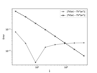
Figure 2: Errors $|\operatorname*{TV}(w)-{\operatorname*{TV}}^{\tau}(w^{\tau})|$ and $|\operatorname*{TV}(w)-\operatorname*{TV^{h}}(w^{\tau})|$ for the pairs $(h,\tau)$ listed in Table 1 with $w^{\tau}=R^{W}_{P0^{\tau}}(w)$.

To demonstrate our theoretical results, we carried out two numerical experiments that were run on a single node of the Linux HPC cluster LiDO3 with CPU 2x Intel Xeon E5-2640v4 and 64 GB RAM. We used DOLFINx 0.7.2 [5] for the finite element discretization and Gurobi 10.0.3 [22] to solve the occurring optimization problems (MIP) and (QP).

The first numerical experiment is concerned with the approximation of $\operatorname*{TV}$ with $\operatorname*{TV^{h}}$. Example 2.10 demonstrated that there are functions $w\in\operatorname*{BV_{W}}(\Omega)$ such that $\operatorname*{TV}(w)$ can not be approximated with ${\operatorname*{TV}}^{\tau}(R^{W}_{P0^{\tau}}(w))$. We solved this issue by discretizing $w$ on a finer mesh than the mesh for the total variation and proved in Theorems 2.9 and 2.14 that we can approximate $\operatorname*{TV}(w)$ with $\operatorname*{TV^{h}}(R^{W}_{P0^{\tau}}(w))$ when the meshes $\mathcal{Q}_{h}$ and $\mathcal{Q}_{\tau}$ are coupled such that $\frac{\tau}{h}\searrow 0$ as $h\searrow 0$ and Assumption 2.3 is fulfilled. We take up Example 2.10 and consider the function $w=\chi_{\{(\frac{1}{3},-1)^{T}x\geq 0\}}\in\operatorname*{BV_{W}}(\Omega)$ with $\Omega=(0,1)^{2}$ and $W=\{0,1\}$. We discretized $\Omega$ into meshes $\mathcal{Q}_{h}$ and $\mathcal{Q}_{\tau}$ of axis-aligned squares for decreasing $h$ and $\tau$ fulfilling Assumption 2.3, see Table 1. We computed the values ${\operatorname*{TV}}^{\tau}(w^{\tau})$ and $\operatorname*{TV^{h}}(w^{\tau})$ with $w^{\tau}\coloneqq R^{W}_{P0^{\tau}}(w)$. As predicted, we perceive that ${\operatorname*{TV}}^{\tau}(w^{\tau})\to\frac{1+\sqrt{5}}{3}\approx 1.07869>\operatorname*{TV}(w)$ as $\tau\searrow 0$ and $\operatorname*{TV^{h}}(w^{\tau})\to\operatorname*{TV}(w)=\frac{\sqrt{10}}{3}\approx 1.05409$ as $h\searrow 0$. Moreover, we observe an experimental error $\operatorname*{TV}(w)-\operatorname*{TV^{h}}(w^{\tau})\leq r\,\frac{\tau}{h}$ with $r\approx 8.513\cdot 10^{-3}$, see Table 1, in accordance with our theoretical error estimates in Propositions 2.15 and 2.13. Another advantage of using two varying meshes for the input functions and the total variation besides the approximation is that the computation of $\operatorname*{TV^{h}}(w^{\tau})$ is faster than the computation of ${\operatorname*{TV}}^{\tau}(w^{\tau})$ for the same $\tau>0$, which is due to the smaller size of the optimization problem one needs to solve to compute $\operatorname*{TV^{h}}(w^{\tau})$ compared to ${\operatorname*{TV}}^{\tau}(w^{\tau})$. For $h^{-1}=256$ and $\tau^{-1}=256\cdot 16$, we needed $831.16$ seconds to compute $\operatorname*{TV^{h}}(w^{\tau})$ and $30933.33$ seconds to compute ${\operatorname*{TV}}^{\tau}(w^{\tau})$.

As a second numerical example, we consider (P) with the choices $F(w)=\|w-w_{d}\|_{L^{1}(\Omega)}$ and $\alpha=5\cdot 10^{-3}$ , that is, we consider the imaging optimization problem

$$\begin{aligned} \min_{w\in L^{2}(\Omega)}\ &\|w-w_{d}\|_{L^{1}(\Omega)}+0.005\operatorname*{TV}(w)\\ \text{s.t.}\quad&w(x)\in W\subset\mathbb{Z}\text{ for a.a.\ }x\in\Omega,\end{aligned}$$ (P_I)

where $w_{d}\in L^{1}(\Omega)$ represents a noisy image. To keep the problem computationally manageable with an off-the-shelf solver, we decided to measure the distance between $w$ and $w_{d}$ in the $L^{1}$-norm instead of the more common $L^{2}$-norm because the $L^{1}$-norm yields mixed-integer linear programs after discretization. This is also the problem class that arises as subproblems in [29], but since the subproblems have additional constraints which make them computationally more expensive, we leave them as future work. The original picture is shown in Fig. 3 (a) and the noisy version is shown in Fig. 3 (b). To obtain $w_{d}$, we added Gaussian noise with standard deviation $\sigma=5\%$ to the original picture and scaled the gray scale values to the interval $[0,5]$. We set $W=\{0,\dots,5\}$ which represents six evenly distributed gray scale values.

For the discretization (P${}^{h}_{c}$) of the problem above, we chose the mesh sizes $(h,\tau)=(\frac{1}{32},\frac{1}{128})$ and $(h,\tau)=(\frac{1}{64},\frac{1}{512})$ and the constants $c=3^{i}\sqrt{2}$ with $i=0,\dots,4$. We applied Algorithm 1 with an iteration limit of $25$ iterations and a tolerance of ${10}^{-03}$ for the gap $\frac{\operatorname*{TV^{h}}(w)-V}{\operatorname*{TV^{h}}(w)}$. We set the time limit for Gurobi to solve the mixed-integer linear programs (MIP) to $48$ hours and the acceptable optimality gap to the default value ${10}^{-04}$. We present the results for the case $(h,\tau)=(\frac{1}{32},\frac{1}{128})$ in Table 2 and for the case $(h,\tau)=(\frac{1}{64},\frac{1}{512})$ in Table 3. In the tables, we provide the respective value of the constant $c$, the information why the algorithm terminated, the number of iterations until termination, the objective value, the values $\operatorname*{TV}(w)$, $\operatorname*{TV^{h}}(w)$, $V$, the gap $\frac{\operatorname*{TV^{h}}(w)-V}{\operatorname*{TV^{h}}(w)}$ of the last iterate $(w,V)$, and the running time in seconds. In column $2$ of Tables 2 and 3, the abbreviations indicate the reason for the termination of the algorithm, where Opt means that we have found an optimal solution, Tol means that that $\frac{\operatorname*{TV^{h}}(w)-V}{\operatorname*{TV^{h}}(w)}\leq 10^{-3}$, MaxIter means that Algorithm 1 reached the iteration maximum, and GrbTime means that Gurobi reached the time limit while solving (MIP). The resulting images for the case $(h,\tau)=(\frac{1}{64},\frac{1}{512})$ as well as the original and the noisy image are shown in Fig. 3.

In our numerical experiments, we observed that Algorithm 1 was mostly able to close the gap between $V$ and $\operatorname*{TV^{h}}(w)$ within the first few iterations to an accuracy of order ${10}^{-02}$ but it was not able to close the gap to the desired accuracy of ${10}^{-03}$ within the prescribed iteration limit of $25$ iterations. Further experiments suggest that a moderate increase of the iteration limit is not sufficient to achieve an accuracy of ${10}^{-03}$ in this example.

We highlight the impact of the choice of the constant $c$ in Fig. 3 for the discretized problems (P${}^{h}_{c}$), even if the specific choice of $c\geq\sqrt{2}$ does not make a difference in the limit from a theoretical point of view. In Fig. 3 (c), we chose the constant $c=\sqrt{2}$ from Theorem 3.13 and in Fig. 3 (e) the constant $c=9\sqrt{2}$ from Theorem 3.12 which leads to significantly different results. In particular, the constraint $\operatorname*{TV}(w)\leq cV$ for smaller $c$ filters out chattering as we obtained for $c=9\sqrt{2}$ and $c=27\sqrt{2}$ in Fig. 3 (e) and (f). This might also avoid effects as observed in Figure 11 in [14], where the authors detected diffuse solutions to an inpainting problem discretized with the Raviart–Thomas approach from [10].

Table 1: Values of $h^{-1}$, $\tau^{-1}$, ${\operatorname*{TV}}^{\tau}(w^{\tau})$, and $\operatorname*{TV^{h}}(w^{\tau})$ with $w^{\tau}=R^{W}_{P0^{\tau}}(w)$.

$h^{-1}$	$\tau^{-1}$	${\operatorname*{TV}}^{\tau}(w^{\tau})$	$\operatorname*{TV^{h}}(w^{\tau})$	$\operatorname*{TV}(w)$	$(\operatorname*{TV}(w)-\operatorname*{TV^{h}}(w^{\tau}))\frac{h}{\tau}$
2	$2\cdot 9$	0.97748	0.36456	1.05409	$8.513\text{\times}{10}^{-03}$
4	$4\cdot 10$	1.03118	0.67116	1.05409	$2.292\text{\times}{10}^{-03}$
8	$8\cdot 11$	1.05709	0.86291	1.05409	$2.727\text{\times}{10}^{-04}$
16	$16\cdot 12$	1.0692	0.95678	1.05409	$1.259\text{\times}{10}^{-03}$
32	$32\cdot 13$	1.07393	1.00593	1.05409	$1.526\text{\times}{10}^{-03}$
64	$64\cdot 14$	1.07648	1.02999	1.05409	$1.599\text{\times}{10}^{-03}$
128	$128\cdot 15$	1.07774	1.04208	1.05409	$1.577\text{\times}{10}^{-03}$
256	$256\cdot 16$	1.07822	1.04805	1.05409	$1.508\text{\times}{10}^{-03}$

(a) Original

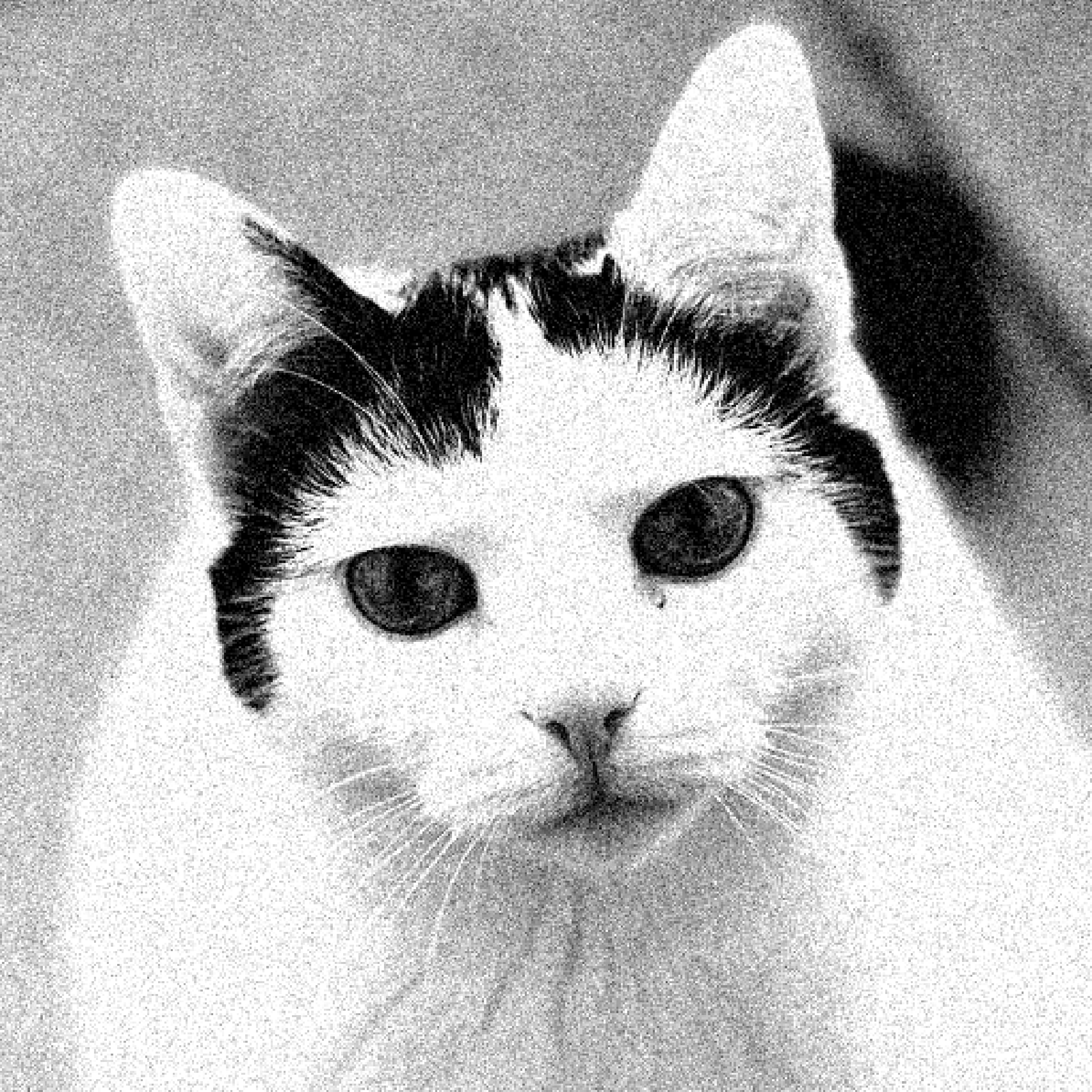
(b) Noisy

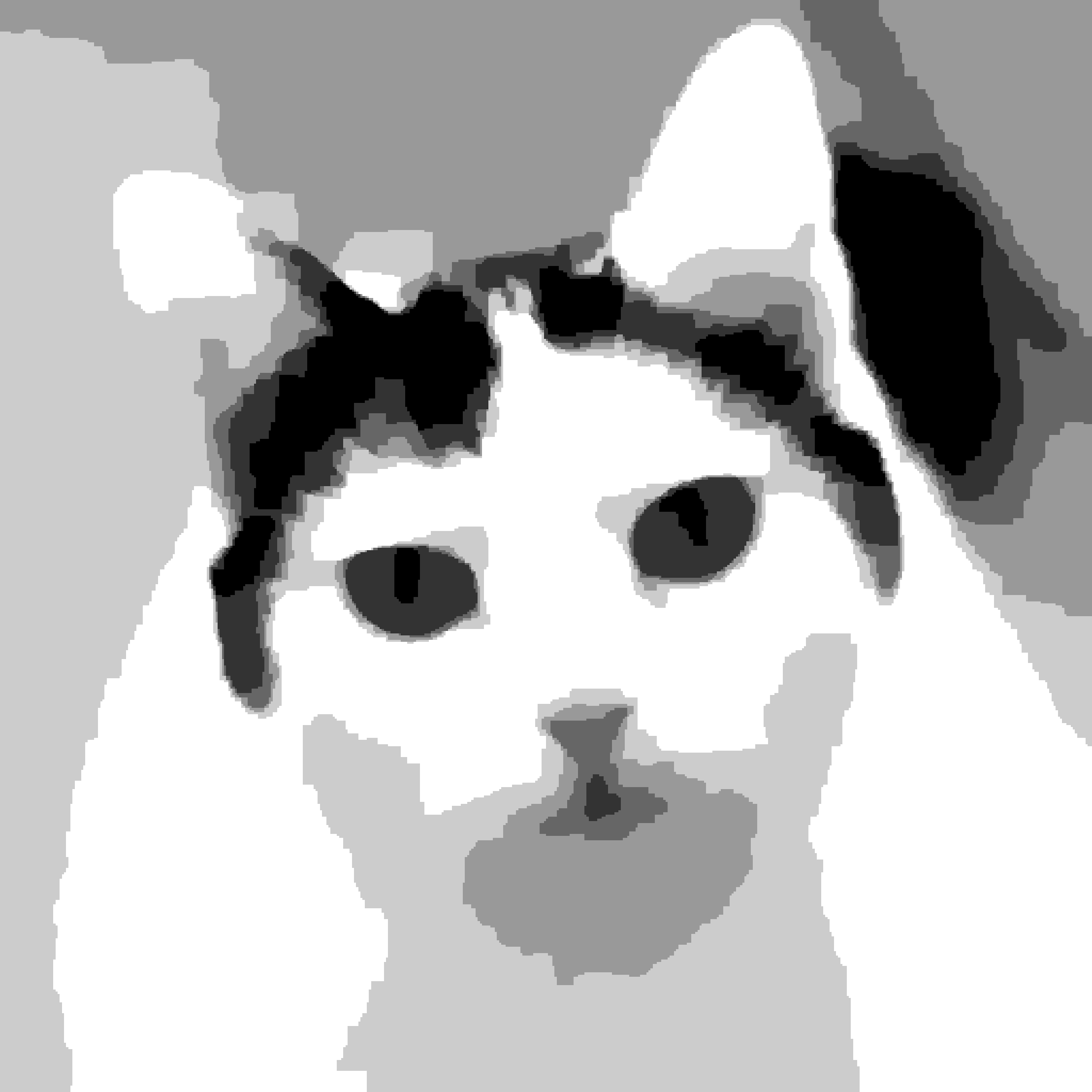
(c) $c=\sqrt{2}$

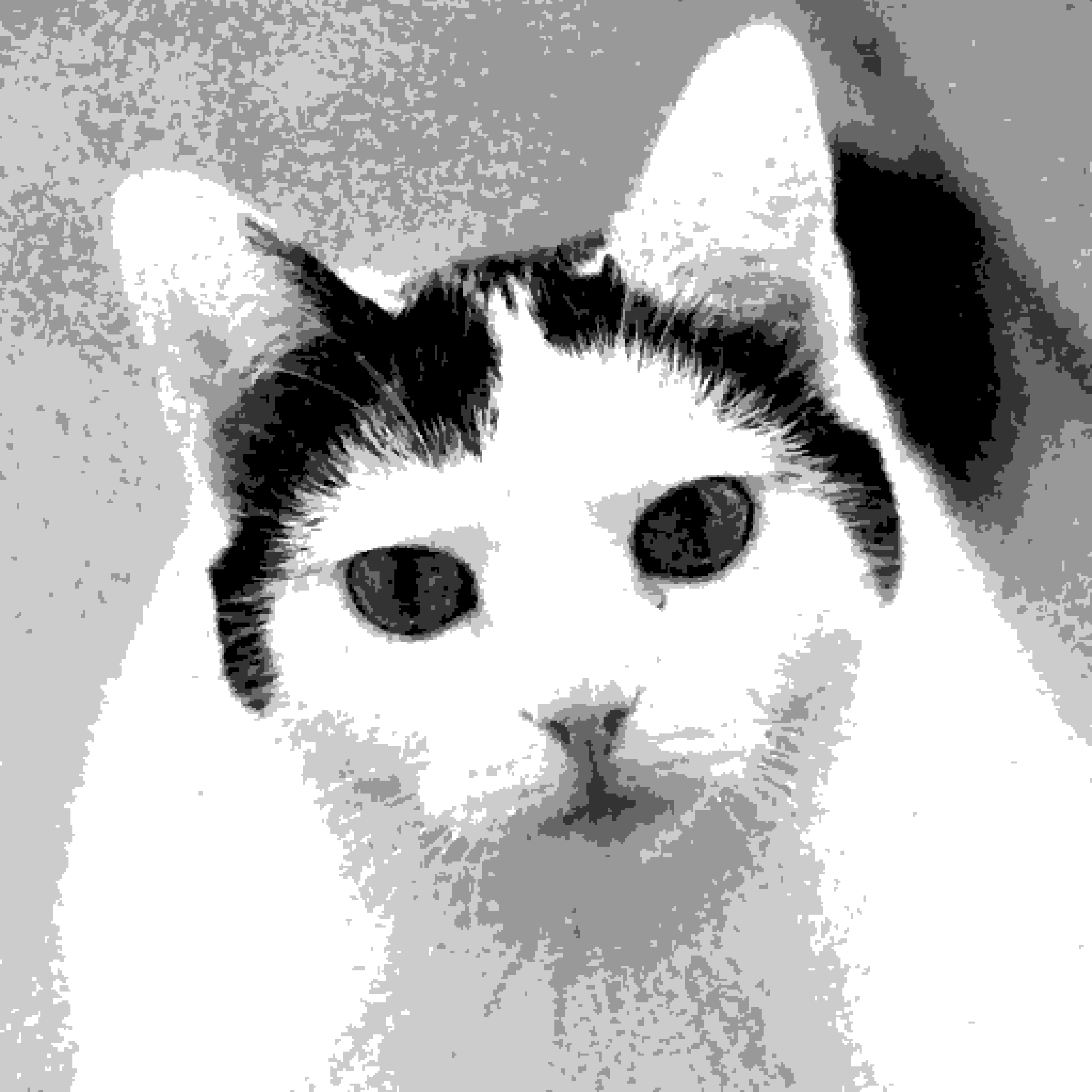
(d) $c=3\sqrt{2}$

(e) $c=9\sqrt{2}$

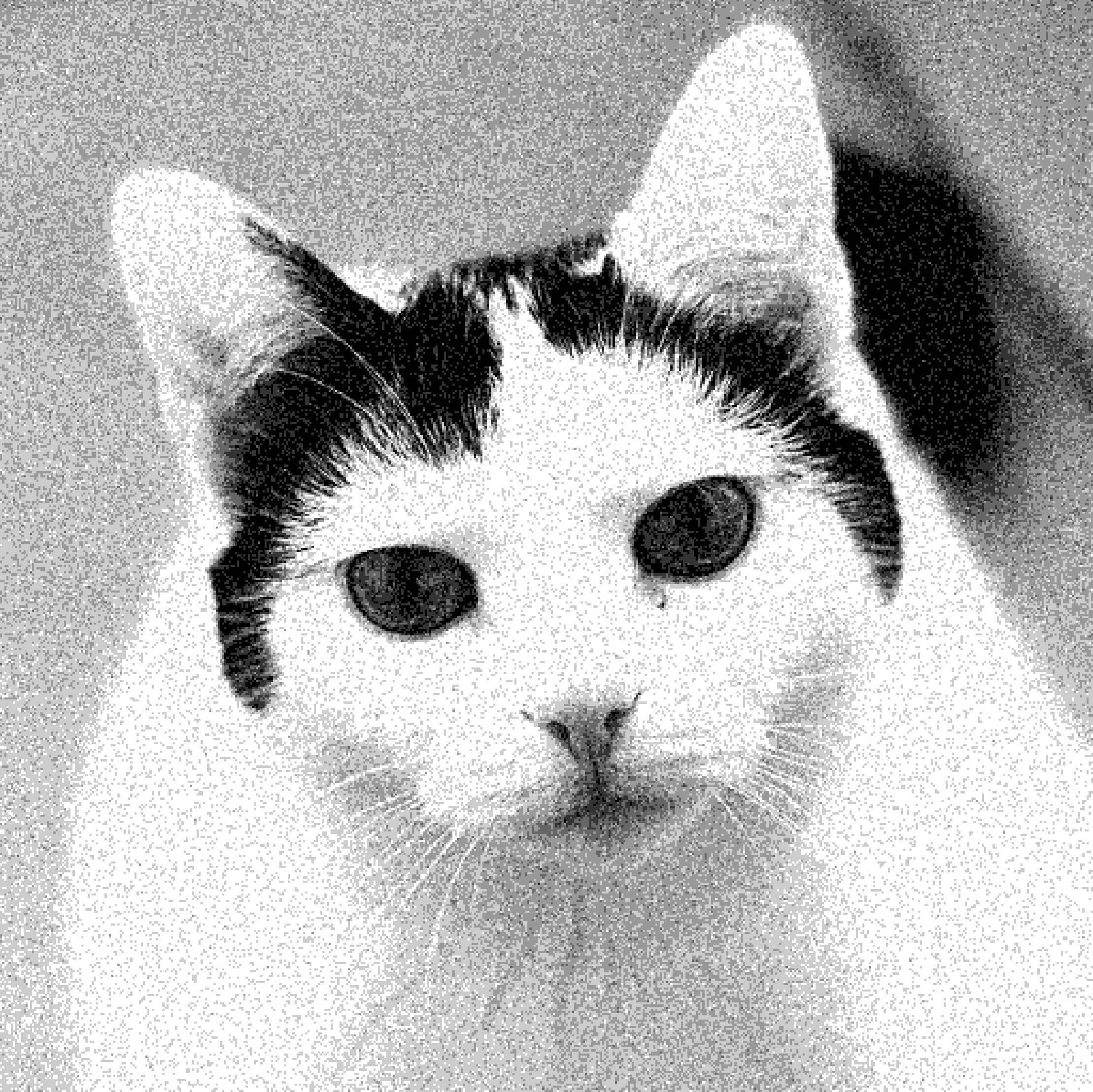
(f) $c=27\sqrt{2}$

Figure 3: Original image, noisy image, and resulting images obtained by applying Algorithm 1 to the discretization of (P_I) with $(h,\tau)=(\frac{1}{64},\frac{1}{512})$ and different values $c$.

Table 2: Results from the application of Algorithm 1 to (P${}^{h}_{c}$) resulting from (P_I) with $(h,\tau)=(\frac{1}{32},\frac{1}{128})$.

$c$	Term.	It.	Obj. val.	$\operatorname*{TV}$	$\operatorname*{TV^{h}}$	$V$	Gap	Time (s)
$\sqrt{2}$	Opt	1	0.453581	34.546875	19.985456	24.428330	$-2.223\text{\times}{10}^{-01}$	28
$3\sqrt{2}$	Tol	24	0.328303	89.679688	21.143576	21.137705	$2.777\text{\times}{10}^{-04}$	7613
$9\sqrt{2}$	MaxIter	25	0.297379	135.218750	18.054645	17.843617	$1.169\text{\times}{10}^{-02}$	2154
$27\sqrt{2}$	MaxIter	25	0.297393	135.132813	17.967840	17.798740	$9.411\text{\times}{10}^{-03}$	1502
$81\sqrt{2}$	MaxIter	25	0.297377	135.140625	17.973196	17.782075	$1.063\text{\times}{10}^{-02}$	1786

Table 3: Results from the application of Algorithm 1 to (P${}^{h}_{c}$) resulting from (P_I) with $(h,\tau)=(\frac{1}{64},\frac{1}{512})$.

$c$	Term.	It.	Obj. val.	$\operatorname*{TV}$	$\operatorname*{TV^{h}}$	$V$	Gap	Time (s)
$\sqrt{2}$	GrbTime	9	0.498596	29.820312	21.295309	21.086300	$9.815\text{\times}{10}^{-03}$	343893
$3\sqrt{2}$	GrbTime	13	0.437718	97.527344	24.093675	22.987415	$4.591\text{\times}{10}^{-02}$	384429
$9\sqrt{2}$	MaxIter	25	0.343889	301.912109	24.076626	23.721174	$1.476\text{\times}{10}^{-02}$	539392
$27\sqrt{2}$	MaxIter	25	0.307785	464.355469	21.445615	20.954688	$2.289\text{\times}{10}^{-02}$	515671
$81\sqrt{2}$	Tol	5	0.312697	491.566406	22.357736	22.357736	$0.000\text{\times}{10}^{00}$	35436

6 Conclusion and outlook

We have introduced a two-level discretization of infinite-dimensional optimization problems with integrality constraints and total variation regularization, where the dual formulation of the total variation is discretized by means of Raviart–Thomas functions on a coarser mesh and the input function is discretized on an embedded mesh. A superlinear coupling of the mesh sizes has an averaging effect that enables to recover the total variation of an integer-valued function by the discretized total variation of an integer-valued recovery sequence. We added a constraint to the discretized problems that vanishes in the limit and which ensures the compactness of the sequence of minimizers of the discretized problems. Together, this ensures the convergence of these minimizers to a minimizer of the original problem. For the solution of the discretized problems, we introduced an outer approximation algorithm. We provided two numerical examples which confirm our theoretical results. As future work, we want to apply the developed discretization to the trust-region subproblems from [29] and solve them using acceleration techniques for integer programs. Since the exact knowledge of the constant $c$ paid off in practice, we believe that it is worthwhile to extent the proof of the two-dimensional case to the three-dimensional case as future research.

Appendix A Proof of Theorem 3.13

We present the arguments that are needed for the proof of Theorem 3.13 and eventually the detailed proof of Theorem 3.13. The first result is due to [8] and states that each function in $\operatorname*{BV_{W}}(\Omega)$ can be approximated by a strictly converging sequence in $\operatorname*{BV_{W}}(\Omega)$ of functions with polygonal level sets. In line with [8], we first define polygonal sets for $d=2$.

Definition A.1.

Let $d=2$. We say that a set $\Sigma\subset\Omega$ is polygonal if there is a finite number of closed line segments $S_{1},\dots,S_{n}\subset\mathbb{R}^{2}$ of strictly positive $\mathcal{H}^{1}$-measure such that $\Sigma$ coincides, up to $\mathcal{H}^{1}$-null sets, with $\bigcup_{j=1}^{n}S_{j}\cap\Omega$. We call a point in which at least two line segments intersect or a line segment ends a vertex.

Lemma A.2.

Let $w\in\operatorname*{BV_{W}}(\Omega)$. There is a sequence $\{w^{k}\}_{k\in\mathbb{N}}\subset\operatorname*{BV_{W}}(\Omega)$ of functions with level sets with polygonal boundaries such that $w^{k}\to w$ in $L^{1}(\Omega)$ and $\operatorname*{TV}(w^{k})\to\operatorname*{TV}(w)$.

Proof.

Follows from Theorem 2.1 and Corollary 2.5 in [8]. Note that $\Omega$ is bounded in our setting and we do not need to work with $L^{1}_{loc}(\Omega)$ here. ∎

For $w\in\operatorname*{BV_{W}}(\Omega)$ with jumpsets with polygonal boundary, we are able to bound the limit of $\operatorname*{TV}(R^{W}_{P0^{\tau}}(w))$ for $\tau\searrow 0$ from above by $\sqrt{2}\operatorname*{TV}(w)$.

Theorem A.3.

Let $d=2$, $\{\mathcal{Q}_{\tau}\}_{\tau>0}$ partitions of $\Omega$ fulfilling Assumption 2.3, and $w\in\operatorname*{BV_{W}}(\Omega)$ be such that the level sets of $w$ have polygonal boundaries. Then there holds

$$\limsup_{\tau\searrow 0}\operatorname*{TV}(R^{W}_{P0^{\tau}}(w))\leq\sqrt{2}\operatorname*{TV}(w).$$

Figure 4: Example for a function $w\in\operatorname*{BV_{W}}(\Omega)$ with level sets that have polygonal boundaries with the notations from the proof of Theorem A.3.

Proof.

Let $w\in\operatorname*{BV_{W}}(\Omega)$ have level sets with polygonal boundaries consisting of $n\in\mathbb{N}$ line segments. We denote the set of these line segments by $\mathcal{S}$ and the associated set of vertices by $V$. We may assume without loss of generality that the line segments in $\mathcal{S}$ do not contain vertices in their relative interior, i.e., one line segment connects exactly two adjacent vertices. This yields that the number of vertices is also bounded by twice the number of line segments $n$. Moreover, a line segment $S\in\mathcal{S}$ separates exactly two level sets inside $\Omega$ and we may restrict the line segments to $\bar{\Omega}$.

We make the following preliminary considerations: consider a ball $B_{\varepsilon}(v)$ with radius $\varepsilon>0$ centered at a vertex $v\in V$. Denote by $\alpha\in(0,\pi]$ the angle between two segments $S_{1},S_{2}\in\mathcal{S}$ with $S_{1}\neq S_{2}$ meeting in $v$. The distance $\delta\geq 0$ between the two points $\partial B_{\varepsilon}(v)\cap S_{1}$ and $\partial B_{\varepsilon}(v)\cap S_{2}$ is then given by $\delta=\varepsilon s$, where we define $s\coloneqq 2\sin\left(\frac{\alpha}{2}\right)$. Let the mesh size $\tau>0$ be small enough such that there hold $\partial B_{\varepsilon}(v)\cap S_{1}\neq\emptyset$ and $\partial B_{\varepsilon}(v)\cap S_{2}\neq\emptyset$ with $\varepsilon\coloneqq\left(1+\frac{1}{s}\right)\sqrt{2}\tau$. Then there holds $\delta>\sqrt{2}\tau$, that is $\partial B_{\varepsilon}(v)\cap S_{1}$ and $\partial B_{\varepsilon}(v)\cap S_{2}$ do not lie in the same cube $Q\in\mathcal{Q}_{\tau}$. The number of cubes of a given mesh $\mathcal{Q}_{\tau}$ that intersect the ball $B_{\varepsilon}(v)$ can be bounded from above by $\frac{4(\varepsilon+\tau)^{2}}{\tau^{2}}$ so that we obtain for our choice of $\varepsilon$ the upper bound $b\coloneqq 16\left(\frac{1}{\sqrt{2}}+1+\frac{1}{s}\right)$ which is constant and independent of $\tau$ and $\varepsilon$.

Now let $\alpha\in(0,\pi]$ denote the minimum angle between two segments meeting in a vertex $v\in V$ and define $\varepsilon$ as above. We consider the line segments $\mathcal{S}^{\varepsilon}\coloneqq\left\{S\setminus\cup_{v\in V}B_{\varepsilon}(v)\mid S\in\mathcal{S}\right\}$ outside the balls $B_{\varepsilon}(v)$. The number of segments in $\mathcal{S}^{\varepsilon}$ is then for $\tau$ small enough equal to $n$. Moreover, by the choice of $\varepsilon$, there is no cube $Q\in\mathcal{Q}_{\tau}$ that contains more than one line segment from $\mathcal{S}^{\varepsilon}$.

We make the following observations. The reduced boundary of the level sets of $R^{W}_{P0^{\tau}}(w)$ is by Definition 2.11 a subset of the boundaries of the cells of $\mathcal{Q}_{\tau}$. Because the total variation of a $W$-valued function is the sum of the interface lengths weighted by their respective jump heights, we can split $\operatorname*{TV}(R^{W}_{P0^{\tau}}(w))$ into a contribution along segments from $\mathcal{S}^{\varepsilon}$ and a contribution inside the balls $B_{\varepsilon}(v)$.

We estimate the contribution inside the balls conservatively by multiplying the number of cubes inside the balls with their perimeter, that is in total by $4bn\tau$.

Now let a segment $S=\operatorname{conv}\{u,v\}\in\mathcal{S}^{\varepsilon}$ with $u,v\in\Omega$ be given. Then we can bound the contribution to $\operatorname*{TV}(R^{W}_{P0^{\tau}}(w))$ along $S$ from above by $(\|u-v\|_{1}+4\tau)|w_{1}-w_{2}|\leq(\sqrt{2}\|u-v\|_{2}+4\tau)|w_{1}-w_{2}|$, where $w_{1},w_{2}\in W$ denote the two values of $w$ within the two level sets separated by $S$. The estimate holds because the value of $R^{W}_{P0^{\tau}}(w)$ on a cube along $S$ is determined solely by the value of $w$ in the center point of the cube and by the monotonicity of the line segment $S$. Since the total variation of $w$ along $S$ is given by $|w_{1}-w_{2}|\|u-v\|_{2}$, we conclude $\operatorname*{TV}(R^{W}_{P0^{\tau}}(w))\leq\sqrt{2}\operatorname*{TV}(w)+4n(W_{\max}+b)\tau$ with $W_{\max}\coloneqq\max_{w_{1},w_{2}\in W}|w_{1}-w_{2}|$ so that $\limsup_{\tau\searrow 0}\operatorname*{TV}(R^{W}_{P0^{\tau}}(w))\leq\sqrt{2}\operatorname*{TV}(w)$. ∎

Finally, we provide the proof of Theorem 3.13.

Proof of Theorem 3.13.

By Lemma A.2, there is a sequence $\{v^{j}\}_{j\in\mathbb{N}}\subset\operatorname*{BV_{W}}(\Omega)$ of functions with jump sets with polygonal boundaries such that $v^{j}\to w$ in $L^{1}(\Omega)$ and $\operatorname*{TV}(v^{j})\to\operatorname*{TV}(w)$ as $j\to\infty$. We pick a subsequence $\{v^{j_{m}}\}_{m\in\mathbb{N}}$ such that we have $\|v^{j_{m}}-w\|_{L^{1}(\Omega)}\leq\frac{1}{m}$ and $\operatorname*{TV}(v^{j_{m}})\leq\operatorname*{TV}(w)+\frac{1}{m}$. By Lemma 2.12, there holds $R^{W}_{P0^{\tau_{h}}}(v^{j_{m}})\to v^{j_{m}}\text{ as }h\searrow 0\text{ in }L^{1}(\Omega)$. Since the functions $\{v^{j_{m}}\}_{m\in\mathbb{N}}$ have jump sets with polygonal boundaries, we may apply Theorem A.3 such that there holds $\limsup_{h\searrow 0}\operatorname*{TV}(R^{W}_{P0^{\tau_{h}}}(v^{j_{m}}))\leq\sqrt{2}\operatorname*{TV}(v^{j_{m}})$. This yields that for each $m\in\mathbb{N}$ there is some $h_{m}>0$ such that $\|R^{W}_{P0^{\tau_{h}}}(v^{j_{m}})-v^{j_{m}}\|_{L^{1}(\Omega)}\leq\frac{1}{m}$ and $\operatorname*{TV}(R^{W}_{P0^{\tau_{h}}}(v^{j_{m}}))\leq\sqrt{2}\operatorname*{TV}(v^{j_{m}})+\frac{1}{m}$ for all $h\leq h_{m}$. We additionally choose the sequence $\{h_{m}\}_{m\in\mathbb{N}}$ such that it decreases strictly monotonically. We define $\{\tilde{w}^{h}\}_{h>0}$ by $\tilde{w}^{h}\coloneqq v^{j_{m}}$ for $h\in(h_{m+1},h_{m}]$ and $w^{h}\coloneqq R^{W}_{P0^{\tau_{h}}}(\tilde{w}^{h})$ for $h>0$. There holds for $h\in(h_{m+1},h_{m}]$ that

$$\|w^{h}-w\|_{L^{1}(\Omega)} =\|R^{W}_{P0^{\tau_{h}}}(\tilde{w}^{h})-w\|_{L^{1}(\Omega)}=\|R^{W}_{P0^{\tau_{h}}}(v^{j_{m}})-w\|_{L^{1}(\Omega)}$$

$$\leq\|R^{W}_{P0^{\tau_{h}}}(v^{j_{m}})-v^{j_{m}}\|_{L^{1}(\Omega)}+\|v^{j_{m}}-w\|_{L^{1}(\Omega)}\leq\frac{2}{m},$$

and

$$\operatorname*{TV}(w^{h}) =\operatorname*{TV}(R^{W}_{P0^{\tau_{h}}}(\tilde{w}^{h}))=\operatorname*{TV}(R^{W}_{P0^{\tau_{h}}}(v^{j_{m}}))$$

$$\leq\sqrt{2}\operatorname*{TV}(v^{j_{m}})+\frac{1}{m}\leq\sqrt{2}\operatorname*{TV}(w)+\frac{1+\sqrt{2}}{m}.$$

That is, for each $m\in\mathbb{N}$ there hold $\|w^{h}-w\|_{L^{1}(\Omega)}\leq\frac{2}{m}$ and $\operatorname*{TV}(w^{h})\leq\sqrt{2}\operatorname*{TV}(w)+\frac{1+\sqrt{2}}{m}$ for all $h\leq h_{m}$, which yields $w^{h}\to w$ in $L^{1}(\Omega)$ as $h\searrow 0$ and $\limsup_{h\searrow 0}\operatorname*{TV}(w^{h})$ $\leq\sqrt{2}\operatorname*{TV}(w)$. In particular, the sequence $\{w^{h}\}_{h>0}$ is bounded in $\operatorname*{BV}(\Omega)$, which together with the convergence in $L^{1}(\Omega)$ yields that $w^{h}\stackrel{{\scriptstyle\ast}}{{\rightharpoonup}}w$ as $h\searrow 0$ in $\operatorname*{BV}(\Omega)$.

Moreover, by Proposition 2.13, for each $m\in\mathbb{N}$ there holds for all $h\in(h_{m+1},h_{m}]$

$$\operatorname*{TV^{h}}(w^{h}) =\operatorname*{TV^{h}}(R^{W}_{P0^{\tau_{h}}}(v^{j_{m}}))$$

$$\leq\left(1+\frac{4\sqrt{2}\tau_{h}}{h}\right)\operatorname*{TV}(v^{j_{m}})\leq\left(1+\frac{4\sqrt{2}\tau_{h}}{h}\right)\left(\operatorname*{TV}(w)+\frac{1}{m}\right),$$

such that $\limsup_{h\searrow 0}\operatorname*{TV^{h}}(w^{h})\leq\operatorname*{TV}(w)$ due to $\frac{\tau_{h}}{h}\searrow 0$ as $h\searrow 0$. ∎

References

[1]
R. Abergel and L. Moisan.
The Shannon total variation.
Journal of Mathematical Imaging and Vision, 59(2):341–370,
2017.
[2]
G. Acosta, T. Apel, R. Durán, and A. Lombardi.
Error estimates for Raviart–Thomas interpolation of any order on
anisotropic tetrahedra.
Mathematics of Computation, 80(273):141–163, 2011.
[3]
L. Ambrosio, N. Fusco, and D. Pallara.
Functions of Bounded Variation and Free Discontinuity Problems,
volume 254 of Oxford Mathematical Monographs.
Clarendon Press Oxford, 2000.
[4]
C. Bahriawati and C. Carstensen.
Three Matlab implementations of the lowest-order
Raviart–Thomas mfem with a posteriori error control.
Comput. Methods Appl. Math., 5:333–361, 2005.
[5]
I. A. Baratta, J. P. Dean, J. S. Dokken, M. Habera, J. S. Hale, C. N.
Richardson, M. E. Rognes, M. W. Scroggs, N. Sime, and G. N. Wells.
DOLFINx: the next generation FEniCS problem solving environment.
preprint, 2023.
[6]
S. Bartels.
Total variation minimization with finite elements: Convergence and
iterative solution.
SIAM Journal on Numerical Analysis, 50(3):1162–1180, 2012.
[7]
S. Bartels, R. H. Nochetto, and A. J. Salgado.
Discrete total variation flows without regularization.
SIAM Journal on Numerical Analysis, 52(1):363–385, 2014.
[8]
A. Braides, S. Conti, and A. Garroni.
Density of polyhedral partitions.
Calculus of Variations and Partial Differential Equations,
56(2):28, 2017.
[9]
F. Brezzi and M. Fortin.
Mixed and Hybrid Finite Element Methods.
Springer New York, NY, 1991.
[10]
C. Caillaud and A. Chambolle.
Error estimates for finite differences approximations of the total
variation.
IMA Journal of Numerical Analysis, 43(2):692–736, 03 2022.
[11]
A. Chambolle, S. E. Levine, and B. J. Lucier.
An upwind finite-difference method for total variation-based image
smoothing.
SIAM Journal on Imaging Sciences, 4(1):277–299, 2011.
[12]
A. Chambolle and P.-L. Lions.
Image recovery via total variation minimization and related problems.
Numerische Mathematik, 76(2):167–188, 1997.
[13]
A. Chambolle and T. Pock.
Crouzeix–Raviart approximation of the total variation on
simplicial meshes.
Journal of Mathematical Imaging and Vision, 62(6):872–899,
2020.
[14]
A. Chambolle and T. Pock.
Approximating the total variation with finite differences or finite
elements.
In Andrea Bonito and Ricardo H. Nochetto, editors, Geometric
Partial Differential Equations - Part II, volume 22 of Handbook of
Numerical Analysis, pages 383–417. Elsevier, 2021.
[15]
A. Chambolle and T. Pock.
Learning consistent discretizations of the total variation.
SIAM Journal on Imaging Sciences, 14(2):778–813, 2021.
[16]
A. Chambolle, P. Tan, and S. Vaiter.
Accelerated alternating descent methods for Dykstra-like problems.
Journal of Mathematical Imaging and Vision, 59(3):481–497,
2017.
[17]
L. Condat.
Discrete total variation: New definition and minimization.
SIAM Journal on Imaging Sciences, 10(3):1258–1290, 2017.
[18]
P. Destuynder, M. Jaoua, and H. Sellami.
A dual algorithm for denoising and preserving edges in image
processing.
Journal of Numerical Mathematics, 15(2):149–165, 2007.
[19]
M. Gerdts.
Solving mixed-integer optimal control problems by
Branch&Bound: A case study from automobile test-driving with gear
shift.
Optimal Control Applications and Methods, 26:1–18,
2005.
[20]
S. Göttlich, A. Potschka, and C. Teuber.
A partial outer convexification approach to control transmission
lines.
Computational Optimization and Applications, 72(2):431–456,
2019.
[21]
S. Göttlich, A. Potschka, and U. Ziegler.
Partial outer convexification for traffic light optimization in road
networks.
SIAM Journal on Scientific Computing, 39(1):B53–B75, 2017.
[23]
F. M. Hante, G. Leugering, A. Martin, L. Schewe, and M. Schmidt.
Challenges in Optimal Control Problems for Gas and Fluid Flow in
Networks of Pipes and Canals: From Modeling to Industrial Applications,
pages 77–122.
Springer Singapore, Singapore, 2017.
[24]
M. Hintermüller, C. N. Rautenberg, and J. Hahn.
Functional-analytic and numerical issues in splitting methods for
total variation-based image reconstruction.
Inverse Problems, 30(5):055014, may 2014.
[25]
M. Hintermüller and C.N. Rautenberg.
On the density of classes of closed convex sets with pointwise
constraints in Sobolev spaces.
Journal of Mathematical Analysis and Applications,
426(1):585–593, 2015.
[26]
M.-J. Lai and L. M. Messi.
Piecewise linear approximation of the continuous
Rudin–Osher–Fatemi model for image denoising.
SIAM Journal on Numerical Analysis, 50(5):2446–2466, 2012.
[27]
S. Leyffer and P. Manns.
Sequential linear integer programming for integer optimal control
with total variation regularization.
ESAIM: Control, Optimisation and Calculus of Variations, 28:66,
2022.
[28]
F. Maggi.
Sets of Finite Perimeter and Geometric Variational Problems: An
Introduction to Geometric Measure Theory.
Number 135. Cambridge University Press, 2012.
[29]
P. Manns and A. Schiemann.
On integer optimal control with total variation regularization on
multidimensional domains.
SIAM Journal on Control and Optimization, 61(6):3415–3441,
2023.
[30]
C. Meyer and A. Schiemann.
Regularization and outer approximation algorithms for optimal control
in BV.
In preparation, 2024.
[31]
L. Modica.
The gradient theory of phase transitions and the minimal interface
criterion.
Archive for Rational Mechanics and Analysis, 98:123–142, 1987.
[32]
J. P. Oliveira, J. M. Bioucas-Dias, and M. A. T. Figueiredo.
Adaptive total variation image deblurring: A
majorization–minimization approach.
Signal Processing, 89(9):1683–1693, 2009.
[33]
T. Pock, A. Chambolle, D. Cremers, and H. Bischof.
A convex relaxation approach for computing minimal partitions.
In 2009 IEEE conference on computer vision and pattern
recognition, pages 810–817. IEEE, 2009.
[34]
L. I. Rudin, S. Osher, and E. Fatemi.
Nonlinear total variation based noise removal algorithms.
Physica D: Nonlinear Phenomena, 60(1-4):259–268, 1992.
[35]
E. M. Stein and R. Shakarchi.
Real analysis: measure theory, integration, and Hilbert spaces.
Princeton University Press, 2005.
[36]
J. Wang and B. J. Lucier.
Error bounds for finite-difference methods for
Rudin–Osher–Fatemi image smoothing.
SIAM Journal on Numerical Analysis, 49(2):845–868, 2011.