Schrödinger eigenfunctions sharing the same modulus and applications to the control of quantum systems
Abstract
In this paper we investigate when linearly independent eigenfunctions of the Schrödinger operator may have the same modulus. General properties are established and the one-dimensional case is treated in full generality. The study is motivated by its application to the bilinear control of the Schrödinger equation. By assuming that the potentials of interaction satisfy a saturation property and by adapting a strategy recently proposed by Duca and Nersesyan, we discuss when the system can be steered arbitrarily fast between energy levels. Extensions of the previous results to quantum graphs are finally presented.
1 Introduction
Consider a controlled (bilinear) quantum system
| (1.1) |
In (1.1), represents the state of the system, evolving in a Hilbert space , and is the control that can take arbitrarily large values.
One of the fundamental questions in quantum control is the following: is it possible to induce a transition from an energy level to another one in arbitrarily small time? Since in (1.1) quantum decoherence is neglected, the model may only be applicable for small times. This is why results of controllability in arbitrarily small time are particularly important for applications.
In the case in which the Hilbert space where is evolving is finite-dimensional, this problem is well understood. Actually small-time controllability is possible if and only if the evaluation at each point of the unit sphere of the Lie algebra generated by the (right-invariant) vector fields of the controlled part is of maximal rank, see for instance [ABGS17, Theorem 2]. As a consequence, small-time controllability is never possible when the operators commute pairwise and in particular when .
The case of an infinite-dimensional Hilbert space could be very different due to the possible unboundedness of . This happens, for instance, for the controlled PDE
| (1.2) |
on a Riemannian manifold . Here is the Laplace–Beltrami operator, is the internal potential, are potentials of interaction, and is the unbounded operator . Notice that in this case we are precisely in the situation in which the multiplication operators commute pairwise.
In the last years, this subject attracted the attention of several researchers. A first example of system of the form (1.1) evolving in an infinite-dimensional space with and in which transitions among energy levels in arbitrarily small time are possible has been presented in [BCC12]. Although very interesting, such an example is academic (, on the circle , ) and for almost ten years it seemed a safe bet that for systems in the form (1.2) such phenomenon never occurs. Several results in this direction have been obtained (see, for instance, [BCT14, BCT18] and [BBS21]).
A surprising result going in the opposite direction was provided more recently by Duca and Nersesyan [DN24], who proved that on the -dimensional torus, for systems of the type (1.2) with , certain transitions among energy levels are possible in arbitrarily small time. In particular it was proven that it is possible to reach states of arbitrarily large energy in arbitrarily small time. This result has been obtained under an assumption on the potentials of interaction called saturation hypothesis (see Section 2.3 for more details). Such type of hypothesis was inspired by a similar one introduced by Agrachev and Sarychev for the control of the Navier–Stokes equations in [AS05] and [AS06].
The result from [DN24] was extended and proven in a simpler form in [CP23]. In particular in that paper examples of systems evolving on manifolds with a topology different from that of the torus were studied.
The techniques developed in [DN24] and [CP23] actually permit to prove that (under the saturation hypothesis) it is possible to steer in arbitrarily small time a state arbitrarily close to a state of the form for some real-valued function .
Then the possibility of making an arbitrarily fast transition among different energy levels is reduced to the problem of the existence of eigenfunctions corresponding to different energy levels that share the same modulus. This is the property that we study in this paper.
To clarify the situation, let us discuss briefly the case of the circle . The eigenvalues of are , The fundamental state () is non-degenerate and corresponds to the real eigenfunction . The other eigenvalues () are double and correspond to the real eigenfunctions and . Although these eigenfunctions do not differ by a factor of phase only, a suitable linear combination in each eigenspace permits to construct eigenfunctions all with modulus :
| (1.3) |
With the technique developed by Duca and Nersesyan, it is possible to induce a transfer of population in arbitrarily small time among the eigenfunctions (1.3). This can be done approximately and suitable potentials of interaction are necessary.
The purpose of this paper is to study whether the presence of linearly independent eigenfunctions sharing the same modulus is a specific feature of this problem or can occur in more general situations.
The structure of the paper is the following.
In Section 2 we give some basic definitions and examples concerning Schrödinger operators having eigenfunctions sharing the same modulus. We then introduce basic concepts about small-time approximate controllability, we introduce the saturation hypothesis and the result by Duca and Nersesyan [DN24]. We then state in Theorem 2.19 a new result concerning small-time approximate controllability between states sharing the same modulus adapted to manifolds with boundary, in the spirit of the ones given by Duca and Nersesyan for the torus [DN24] and Chambrion and Pozzoli for manifolds without boundary [CP23]. The proof that we give in Appendix A generalizes immediately to the case of the graphs studied in Section 4.
In Section 3 we study conditions for Schrödinger operators to admit eigenfunctions sharing the same modulus in the general case and in the one-dimensional case (Section 3.2). Our main result in the one-dimensional case is Theorem 3.6 that we reformulate here for convenience.
Theorem 1.1.
Let be a smooth and connected one-dimensional manifold (possibly with boundary) and a coordinate on . In , consider the Schrödinger operator (with bounded from below and Neumann or Dirichlet boundary conditions if has boundary) that we assume to be self-adjoint and with compact resolvent. If admits two -linearly independent eigenfunctions and sharing the same modulus, then necessarily is a closed curve and , are nowhere vanishing on . If, moreover, , correspond to distinct eigenvalues, then is constant.
One can read this result in the following way: the requirement of the existence of eigenfunctions sharing the same modulus for all eigenvalues gives a topological constraint (the manifold should be the circle) and a condition on the potential that must be constant. However if we are interested in transitions in between the same eigenspace, then non-constant potentials are admitted. See Remark 3.8 for an explicit example.
In the two-dimensional case, we give some new results concerning the sphere , showing that it is possible to induce small-time transitions among states (which are not eigenstates) having different expectation values of the energy (see Proposition 2.7). This fact is new since for the sphere only the possibility of making small-time transitions between states of the type to was known (see [CP23]). For the disk , we also prove that two eigenfunctions of different energy levels cannot share the same modulus while it is possible to find two independent eigenfunctions of the same energy level that share the same modulus, see 2.8. This result is new and leads to the possibility of making small-time transitions among states having the same energy as for the sphere .
Beside the two-dimensional torus, the sphere and the disk , the study of other systems in dimension 2 is complicated by the lack of explicit expressions for the eigenfunctions.
We then study (Section 4) problems that in a sense are intermediate between dimension 1 and 2, namely problems on graphs. Actually graphs are obtained by gluing together one-dimensional manifolds, but their topology is much richer than the topology of one-dimensional manifolds and for certain properties they are more similar to higher dimensional manifolds. See, for instance, the survey [Kuc02] studying spectral properties in thin structures collapsing to a graph.
On graphs we exhibit some new phenomena. We show the existence of graphs for which
there exists an infinite sequence of eigenfunctions corresponding to arbitrarily high energy levels that share the same modulus, but this is not the case for all energy levels. See Section 4.4;
all energy levels but the ground state are degenerate, but there exists no pair of eigenfunctions sharing the same modulus and having different energy levels. See Section 4.5.
Acknowledgements. This work has been partly supported by the ANR project TRECOS ANR-20-CE40-0009, by the ANR-DFG project “CoRoMo” ANR-22-CE92-0077-01, and has received financial support from the CNRS through the MITI interdisciplinary programs.
2 Basic definitions
2.1 The Schrödinger operator on a Riemannian manifold
Let be a smooth and connected manifold of dimension , possibly with boundary, equipped with a Riemannian metric . We assume that , endowed with the Riemannian distance, is complete as a metric space. Let be the Laplace–Beltrami operator on , where is the divergence operator with respect to the Riemannian volume and is the Riemannian gradient. When , we split where is the set of the connected components of .
We define the Hilbert space , where integration is considered with respect to the Riemannian volume. For simplicity, in the following we write for and, similarly, for , . Let be bounded from below, , and define
| (2.1) |
where, for every , is either the trace of on or the trace of on with the outer unit normal vector to . In the sequel, we split , where (respectively, ) corresponds to the set of indices such that is the trace of on (respectively, the trace of on ).
Assumption 2.1.
The unbounded Schrödinger operator is self-adjoint on with compact resolvent.
As a consequence of 2.1, from the spectral theorem (see, e.g., [CR21, Theorem 6.2]), there exists an orthonormal basis of composed of eigenfunctions associated with the sequence of real eigenvalues , that is for every , . Let us first give some examples, that are mainly taken from [Cha84], on which we will focus in the following.
-
1.
Let be the -dimensional torus, be the Euclidean Laplace operator, . The unbounded operator satisfies Assumption 2.1.
-
2.
Let be the two-dimensional sphere equipped with the standard Riemannian metric and be the corresponding Laplace–Beltrami operator. Let . The unbounded operator satisfies Assumption 2.1.
-
3.
Let be a smooth bounded connected domain of , be the Euclidean Laplace operator, be the outer unit normal vector to and . The unbounded operators and satisfy Assumption 2.1.
-
4.
Let , be the Euclidean Laplace operator, be such that . Then the unbounded operator satisfies Assumption 2.1.
Remark 2.2.
Assumption 2.1 does not cover all interesting situations. Consider for instance the Schrödinger operator
If this operator is essentially self-adjoint in (this is a consequence of [RS78], Theorem X.10) and hence this situation is covered by Assumption 2.1 (even if it does not satisfy the standing assumptions, since the metric space endowed with the Euclidean distance is not complete). If this operator is not essentially self-adjoint. Self-adjoint extensions exist, but they do not correspond to boundary conditions of Dirichlet or Neumann type. In other words the latter case is not covered by Assumption 2.1.
2.2 Eigenfunctions sharing the same modulus
The following definition introduces rigorously the key notion of eigenfunctions of the operator sharing the same modulus.
Definition 2.3.
For , two -linearly independent eigenfunctions and are said to share the same modulus if
| (2.2) |
We are interested in different occurrences of eigenfunctions sharing the same modulus:
-
•
For , may admit eigenfunctions sharing the same modulus inside the energy level , that is, there may exist two -linearly independent eigenfunctions in that share the same modulus;
-
•
For , may admit two eigenfunctions and sharing the same modulus and corresponding to different energy levels and ;
-
•
may admit eigenfunctions sharing the same modulus corresponding to all energy levels, that is, there may exist a subsequence of an orthonormal basis of eigenfunctions such that the functions all share the same modulus and such that .
Let us illustrate these notions on some particular examples of Riemannian manifold and operator .
-
1.
Let , , and . The eigenvalues are given by
(2.3) With each one can associate the eigenstates
(2.4) Since all eigenstates share the same modulus (constantly equal to 1) and are linearly independent if , the following proposition holds true.
Proposition 2.4.
The operator admits eigenfunctions sharing the same modulus inside each energy level and corresponding to all energy levels.
-
2.
Let , , and . Denote by , , , the spherical harmonics, i.e., the eigenfunctions of . Then the eigenvalue associated with is and
(2.5) where is the corresponding Legendre polynomial and are the spherical coordinates on .
Proposition 2.5.
For every , , and share the same modulus. As a consequence, for each , admits eigenfunctions sharing the same modulus inside the energy level .
Proof.
Recall that each satisfies
so that
(2.6) Therefore, and share the same modulus. ∎
Remark 2.6.
A natural open question is the following one: for , , do there exist and sharing the same modulus?
The next result tells us that appropriate linear combinations of spherical harmonics can also share the same modulus.
Proposition 2.7.
For every , there exist some constants such that and share the same modulus.
Proof.
Note that and correspond to different energy levels, so the result tells us that an appropriate superposition of spherical harmonics of different energy levels shares the same modulus as an appropriate superposition of spherical harmonics from a single energy level.
-
3.
Let us consider the unit disk . Denote by the Dirichlet–Laplace operator on . From [Hen06, Proposition 1.2.14], the eigenvalues and eigenfunctions of are given by, for every ,
and, for every ,
where is the -th zero of the Bessel function and are the polar coordinates on .
Proposition 2.8.
Let be such that and . Assume that and are eigenfunctions corresponding to and , respectively. Then and do not share the same modulus.
On the other hand, for and , there exist two -linearly independent eigenfunctions given by
(2.7) corresponding to the eigenvalue that share the same modulus.
Proof.
The first part is a standard application of a celebrated result by Siegel [Sie14] stating that and for have no common zeros, together with the simple observation that two eigenfunctions sharing the same modulus also share the same nodal set.
The second part consists in remarking that the eigenfunctions given by (2.7) are -linearly independent. ∎
-
4.
Let , , and be the harmonic oscillator Hamiltonian.
The eigenfunctions of the one-dimensional harmonic oscillator are the Hermite eigenfunctions
(2.8) The eigenvalue corresponding to is and can be written as , where is a polynomial function of degree . In the multi-dimensional case, for , , the Hermite eigenfunctions are given by
(2.9) and corresponds to the eigenvalue .
Proposition 2.9.
Let . For every , , does not admit two eigenfunctions corresponding to the energy levels and that share the same modulus.
Proof.
By contradiction, if and share the same modulus, then , so that and have the same degree, which is not possible when . ∎
Note that 2.9 can also be seen as a consequence of Lemma 3.1 or Theorem 3.6, see below.
Remark 2.10.
A natural open question is: does the result of 2.9 extend to the case ? The difficulty is that in the contradiction argument, we will have
(2.10) An argument based on the degree does not work anymore because a priori one can have cancellations in the previous equality such that the polynomial in the left hand side has the same degree than the polynomial of the right hand side.
Eigenfunctions sharing the same modulus play a special role in the bilinear control of quantum systems, as explained in the next section.
2.3 Bilinear quantum control systems
Let be the potentials of interactions and let us consider the bilinear controlled Schrödinger equation
| (2.11) |
In (2.11), at time , is the state and is the control.
In all the sequel, we also make the following hypothesis.
Assumption 2.11.
For every , .
By combining Assumptions 2.1 and 2.11, we have the following well-posedness result according to [BMS82]. For every , and , there exists a unique mild solution of (2.11), i.e.,
If we assume furthermore that , then, for every , . In the sequel, for and , the associated solution of (2.11) will be denoted by .
For , let us denote
From a controllability point of view, we have the following well-known negative result from [Tur00], based on [BMS82] (see also [BCC20] for extensions to the case of and impulsive controls): For every , the complement of in is dense in , so in particular the interior of in for the topology of is empty. With respect to this result of negative nature for the exact controllability, one may wonder if instead the approximate controllability holds. It is known that (2.11) is approximately controllable in large time, generically with respect to the parameters of the system, see [MS10]. Here, we will mainly focus on the small-time approximate controllability.
Definition 2.12.
An element belongs to the small-time approximately reachable set from , denoted by , if for every , for every , there exists and such that
The characterization of small-time approximately reachable sets for (2.11) is an open problem in general. For instance, the authors in [BCT18] exhibits a minimal time concerning the approximate controllability between particular initial data and final target for (2.11) when . Results in the same spirit were also obtained in [BBS21] by using a WKB method. Nevertheless, there are examples of bilinear systems for which for all , see [BCC12].
In this article, we mainly focus on a weaker notion, that we call small-time isomodulus approximate controllability.
Definition 2.13.
We say that (2.11) is small-time isomodulus approximately controllable from if
The motivation for studying such a notion comes from the recent papers [DN24] and [CP23]. Roughly speaking, in these papers, the authors prove that the small-time isomodulus approximate controllability holds assuming that the potentials of interaction are smooth up to the boundary of and satisfy a suitable saturation property.
Let us investigate for particular examples of Riemannian manifolds , operators , and potentials of interaction when small-time isomodulus approximate controllability holds.
-
1.
In the case where is a torus the following result holds.
Theorem 2.14.
Note that [DN24, Theorem A] actually claims the small-time isomodulus approximate controllability for for but this is due to the eventual presence of the semi-linearity in their equation.
A striking consequence of such a result is that the small-time approximate controllability among particular eigenstates holds.
Corollary 2.15.
In particular, the system can be steered arbitrarily fast from one energy level to any other one. This is due to the fact that for every , and share the same modulus.
-
2.
For the two-dimensional sphere the following result holds.
Theorem 2.16.
As an application, we have the following result, that claims the small-time approximate controllability between particular spherical harmonics.
Note that [CP23, Theorem 3] actually claims (2.12) for and but the proof is still valid for any because of 2.5. The following result is new.
Corollary 2.18.
For every , , there exist some constants such that
One of the contributions of this article is the generalization of [DN24, Theorem A] and [CP23, Theorem 3] to Riemannian manifolds with boundaries, assuming that the potentials of interaction satisfy a saturation property that we describe now.
We assume that and let us define the sequence of subspaces
| (2.13) |
and iteratively
| (2.14) |
Finally, we define
| (2.15) |
Theorem 2.19.
Assume that is dense in . Then, (2.11) is small-time isomodulus approximately controllable.
It is worth mentioning that the proof of [DN24, Theorem A] directly gives Theorem 2.19 when and the proof of [CP23, Theorem 3] directly gives Theorem 2.19 when is a manifold without boundary. Even if the treatment of the boundary is not the most difficult issue, we give a full proof of Theorem 2.19 in Appendix A in an abstract setting for the sake of completeness and for the application to other quantum control systems, in particular on quantum graphs.
As an application of Theorem 2.19, one can then consider the case of the Dirichlet–Laplace operator on the disk.
Corollary 2.20.
Here, the -regularity up to the boundary of the potentials leads to the fact that one can remove the conditions of the stabilization of by the functions in the definitions (2.13) and (2.14) because it is automatically satisfied. This is specific to the homogeneous Dirichlet boundary conditions. It is not the case for homogeneous Neumann boundary conditions.
3 Eigenfunctions sharing the same modulus
3.1 General properties
The goal of this part is to study the implications of having two linearly independent eigenfunctions sharing the same modulus.
Let be as in Assumption 2.1. Notice that we could relax the assumptions on in this section, not requiring its entire spectrum to be discrete, but just focusing on two of its eigenvalues and with corresponding eigenfunctions . By elliptic regularity and Sobolev embeddings, see for instance [GT01, Theorem 7.26, Theorem 9.11], for every one has that and are . The one-dimensional case is specific because, by standard ODE arguments, one can prove that and are .
Let us assume that and share the same modulus . Set and let be such that
| (3.1) |
Notice that both and vanish on and that, by unique continuation, see [Aro57], is dense in . Moreover, for every one has that and are , and even in the one-dimensional case.
Let us observe the following.
Lemma 3.1.
If and are simple and distinct eigenvalues of the Schrödinger operator with corresponding eigenfunctions and , then and cannot share the same modulus.
Proof.
Assume by contradiction that and share the same modulus and let be as in (3.1).
Notice that, since is real-valued, and satisfy
By using that is a simple eigenvalue, we then deduce that and are colinear, that is, up to exchanging the roles of and , there exists such that , i.e., . We therefore deduce that
By using that is open and is continuous on , we then deduce that is constant on each connected component . As a consequence, we obtain that
By using the same argument for , we obtain
Hence, since is nonempty, , contradicting the hypotheses. ∎
Remark 3.2.
One may wonder if the conclusion of Lemma 3.1 still holds true assuming that only is simple. This turns to be false by considering the example of and . Indeed, is a simple eigenvalue with corresponding eigenfunction constantly equal to , while is an eigenvalue of multiplicity with corresponding eigenfunctions and , and the three eigenfunctions obviously share the same modulus.
Corollary 3.3.
Let be a compact connected manifold without boundary of dimension larger than or equal to . Then, generically with respect to the Riemanniann metric, no pair of -linearly independent eigenfunctions of the Laplace–Beltrami operator share the same modulus.
Proof.
This is straightforward application of Lemma 3.1 and the well-known result by Uhlenbeck [Uhl76, Tan79] 111The version of Uhlenbeck’s result given by Tanikawa in [Tan79] provides the formulation in the topology and also covers the case where has nonempty boundary and the Schrödinger operator has Dirichlet boundary conditions. One could therefore extend the statement of Corollary 3.3 accordingly. ensuring that, given a compact connected manifold of dimension larger than or equal to , the set
is residual in the topological space of all smooth Riemannian metrics on endowed with the topology. ∎
Remark 3.4.
Results similar to Corollary 3.3 can be obtained when considering the genericity with respect to the potential (with no restriction on the dimension of ). Indeed, the spectrum of the Schrödinger operator is known to be generically simple with respect to . This general statement requires precise functional analysis setups to be rigorously formulated. For the case of compact connected manifolds without boundary and potentials see [Alb75]. The case of bounded Euclidean domains with Dirichlet boundary conditions and or of full Euclidean spaces with such that can be found in [MS10, Proposition 3.2].
Let us collect in the following result some differential identities satisfied by the modulus and phases of two eigenfunctions sharing the same modulus.
Lemma 3.5.
Let be two eigenfunctions of the Schrödinger operator sharing the same modulus with corresponding eigenvalues . Let , , be as in (3.1). The following elliptic equations are fulfilled
| (3.2) | ||||
| (3.3) |
Moreover,
| (3.4) |
3.2 The one-dimensional case
A noticeable feature of the one-dimensional case is that, locally around each point of , the Riemannian manifold is isometric to an interval in endowed with the Euclidean metric, as it follows by taking an arclength coordinate (see, for instance, [Mil65, Appendix Classifying -dimensional manifolds]). Hence, since is complete, four situations may occur:
-
•
is isometric to the line ,
-
•
is isometric to the half-line ,
-
•
is isometric to a compact interval for some ,
-
•
is a closed curve isometric to the quotient for some .
Moreover, in the arclength-coordinate the metric is constant and the Laplace–Beltrami operator coincides with the second derivative.
The main result of this section is Theorem 3.6 below, stating, in particular, that a one-dimensional manifold admits a pair of eigenfunctions sharing the same modulus and corresponding to different eigenvalues only if and is constant, that is, in the one-dimensional occurrence of the system studied in [DN24].
Theorem 3.6.
If is one-dimensional and the Schrödinger operator admits two -linearly independent eigenfunctions and sharing the same modulus, then necessarily is a closed curve and , are nowhere vanishing on . If, moreover, the two eigenfunctions correspond to distinct eigenvalues, then is constant.
The proof of the previous result is based on the following lemma.
Lemma 3.7.
Let be an interval in and . Assume that and are such that
Then there exist such that and in . Moreover, if , then there exists such that either or in . If, instead, then and there exists such that
| (3.6) |
Proof.
Setting , we have that
Integrating, we deduce that there exists such that
| (3.7) |
Analogously, there exists such that , . Hence, using the equality , we deduce that
| (3.8) |
If then necessarily , meaning that either or in . The latter means that either or is constant.
Let now consider the case . We deduce from (3.8) that and that is constant on , that is, there exists such that , . ∎
Proof of Theorem 3.6.
Let and be two eigenfunctions of sharing the same modulus and corresponding to the eigenvalues and . In particular, and are assumed to be -linearly independent. Let be as in (3.1). Up to taking an arclength coordinate, equations (3.3) and (3.4) read and on . These are the equations for appearing in the statement of Lemma 3.7.
Let us first exclude the case in which has boundary conditions of Neumann type at a point of . Without loss of generality such point is and for some or . Since for every the space of real-valued solutions of with is one-dimensional, then and are both simple and the conclusion follows from Lemma 3.1.
Let us consider now the case . We obtain from Lemma 3.7 that is locally constant on . Since, moreover, is connected and is continuous, then coincides with some constant on . This excludes the case in which has boundary conditions of Dirichlet type at a point of and the case in which is isometric to or to , since otherwise and would not be in . In particular is a closed curve. We also obtain from (3.2) and (3.6) that is constant (globally on ).
Let us now turn to the case where . We claim that does not vanish on . Assume by contradiction that this is not the case and identify isometrically a connected component of with a possibly unbounded interval or , with . Since on and both and are real-valued, we deduce that and are bounded in a right-neighborhood of . By Lemma 3.7, there exists such that on . Since as , it follows from the boundedness of that . Similarly, , yielding that and are constant on a connected component of . Hence and are -linearly dependent on a nonempty open set of , yielding by the unique continuation principle that they are -linearly dependent on . This concludes the contradiction argument proving that does not vanish on (excluding, in particular, the case in which has boundary conditions of Dirichlet type at a point of ).
We are then left to exclude the case where is isometric to . It follows from Lemma 3.7 that either or is constant on . By -linear independence of and we can exclude the case where is constant and we can assume that on with .
Since and are in , then
| (3.9) |
It follows from (3.2) that satisfies
Since is bounded from below, we deduce that there exists such that at every such that . This is in contradiction with (3.9) and the proof is concluded. ∎
Remark 3.8.
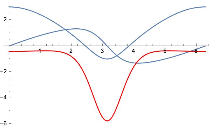
The theorem allows to conclude that is constant only in the case where . Let us see through an example that this is not true in general if . We proceed in a constructive way, starting from any non-constant and selecting and , both non-constant, such that is an eigenfunction of corresponding to the eigenvalue . In particular, and are -linearly independent eigenfunctions of on .
Consider a positive integer to be fixed later and set
It holds by construction that and . Hence , seen as a function from to itself, is well defined and non-constant. Notice that has been defined in such a way that . Setting then
we have that solves
Moreover, can be chosen so that is non-constant.
One can now check that solves . As a consequence, solves the same equation. This completes our construction.
For an explicit example, one can take and
The resulting and the linearly independent eigenfunctions and of are illustrated in Figure 1.
As a consequence of Theorem 2.14 in the case , even in the case it might be possible to steer system (2.11) in arbitrarily small time from one eigenfunction arbitrarily close to a linearly independent one (sharing the same eigenvalue). Notice that the Schrödinger equation on with non-constant potential has a relevant role in solid state physics (see, e.g, [RS78, Section XIII.16]).
4 Quantum graphs
4.1 Setting
Let be a compact connected metric graph with edges of respective lengths and vertices . For every vertex , we denote
| (4.1) |
We denote by the set of internal vertices of , that is, the set of those vertices for which either or and the single edge to which belongs is actually a loop. The remaining vertices are called external and we denote by the set comprising them.
Each edge is parameterized by an arclength coordinate going from to its length . On we consider functions , where for every . We denote
The Hilbert space is equipped with the norm defined by
We then denote by the Sobolev space of all functions on that are continuous (that is, such that if ) and such that belong to for every , equipped with the norm defined by
Finally, the Sobolev space is defined as
equipped with the natural norm.
Let and be a vertex of connected once to an edge with . When the coordinate parameter at the vertex is equal to (respectively, ), we denote
| (4.2) |
When is a loop connected to at both its extremities, we use the notation
| (4.3) |
In the following, we consider two type of boundary conditions. For , we say that satisfies
-
•
a Dirichlet boundary condition at a vertex if ,
-
•
a Neumann–Kirchoff boundary condition at a vertex if .
We partition in a two subsets of vertices and at which we impose, respectively, a Dirichlet and a Neumann–Kirchoff boundary condition.
Let , be the Hamiltonian, and let us define
Definition 4.1.
A quantum graph is a compact connected metric graph , equipped with the unbounded operator .
Given a quantum graph, the Hamiltonian is a self-adjoint operator that has compact resolvent, see [BK13, Theorems 1.4.4 and 3.1.1]. So, there exists an orthonormal basis of eigenfunctions associated with the sequence of real eigenvalues .
4.2 General results for quantum graphs
The definition of eigenfunctions sharing the same modulus is the same as in Definition 2.3.
Lemma 4.2.
If and are simple and distinct eigenvalues of the Hamiltonian with corresponding eigenfunctions and , then and cannot share the same modulus.
Proof.
The proof is analogue to the one of Lemma 3.1. ∎
Corollary 4.3.
Let be a compact graph with the Hamiltonian , equipped with Neumann–Kirchoff conditions. Assume that has at least one vertex with . Then, generically with respect to the lengths of the edges of the graph, no pair of distinct eigenfunctions belonging to the same orthonormal basis of the Laplace–Beltrami operator share the same modulus.
Proof.
Remark 4.4.
Corollary 4.5.
Let be a compact graph with Hamiltonian and Dirichlet boundary conditions at at least one Dirichlet vertex of . Then, there exists a subsequence of eigenfunctions among which no pair share the same modulus.
Proof.
4.3 Bilinear control of the Schrödinger equation in quantum graphs
Let be the -tuple potentials of interaction and let us consider the bilinear controlled Schrödinger equation
| (4.4) |
As for Riemannian manifolds, see Section 2.3, the well-posedness of (2.11) is a consequence of [BMS82]. The notions of mild solutions, reachable sets, controllability are then easily adapted. In particular, we keep the same notations. The interior of for the topology of is empty. For positive results of exact or approximate controllability in subspaces of , we refer to [Duc20] and [Duc21].
Assume that and the restriction of to each edge of is up to the boundary. Let us define as before the sequence of subspaces
| (4.5) |
and by recurrence
| (4.6) |
Finally, we define
| (4.7) |
We have the following result, that is an adaptation of [DN24, Theorem A] in the context of quantum graphs.
Theorem 4.7.
Assume that is dense in . Equation (4.4) is small-time isomodulus approximately controllable, i.e.,
The proof of Theorem 4.7 is given in Section A.3.
In the next two parts, we consider two examples of quantum graphs in which Theorem 4.7 can be applied. In the first example we exhibit a quantum graph with topology different from that of the circle and admitting eigenfunctions that share the same modulus. Each of these eigenfunctions corresponds to an eigenvalue of multiplicity . Note also that in this case the Schrödinger operator admits eigenfunctions corresponding to simple eigenvalues that do not share the same modulus between themselves because of Lemma 4.2 and actually do not share the same modulus with all other eigenfunctions. This highlights the variety of situations that may occur. In the second example we exhibit a quantum graph whose corresponding eigenvalues are all nonsimple (apart from the ground state) and that does not admit eigenfunctions sharing the same modulus and corresponding to different eigenvalues.
For convenience, we use in the following two section the following notation: for every , , , denote the functions defined by
According to this notation, .
4.4 The example of the eight graph
We consider here the compact graph with edges , both of length , with vertex. Namely, is composed of two loops having the same length that are linked to the same vertex, see Figure 2.

We consider the Hamiltonian on and Neumann–Kirchoff boundary conditions at the single vertex.
We have the following result.
Proposition 4.8.
The eigenvalues and eigenfunctions are given by
plus, for every ,
and finally, for ,
Proof.
We know that the eigenvalues are of the form , , because the Hamiltonian operator is nonnegative. As a consequence, on each edge, the eigenfunction is a solution to
So, the eigenfunctions are of the form
We then write the boundary conditions, that are the continuity and the Neumann–Kirchoff conditions at the vertex, leading to
| (4.8) | |||
| (4.9) | |||
| (4.10) | |||
| (4.11) |
If , then we obtain from (4.9) that . We therefore deduce from (4.11) that
Taking into account also (4.10), we find that satisfies the linear system
The determinant of the matrix is different from , leading to .
So necessarily . If with odd, we find that by (4.10) and by the Neumann–Kirchoff condition (4.11) . Finally, if with even, we find that all the conditions are satisfied if , that is, are free parameters. In the case the space parameterized by is one-dimensional, otherwise it has dimension 3.
To conclude, we have that , odd, is a simple eigenvalue with corresponding eigenfunction and , even, corresponds either to a simple eigenvalue for or to an eigenvalue of multiplicity for , associated with eigenfunctions of the type , . ∎
Proposition 4.9.
For every , , there exists an eigenfunction corresponding to and an eigenfunction corresponding to that share the same modulus.
For every , there exist two -linearly independent eigenfunctions corresponding to that share the same modulus.
For every , , two eigenfunctions corresponding to and do not share the same modulus.
For every , , two eigenfunctions corresponding to and do not share the same modulus.
Proof.
For the first point, let us remark that, for ,
so that .
For the second point, let us notice that
For the third point, we use the fact that the eigenvalues are simple and Lemma 4.2.
For the fourth point, let us argue by contradiction. Assume that there exist , , such that
Taking leads to and then taking one gets a contradiction. ∎
We define the potentials
We have the following lemma.
Lemma 4.10.
The set is dense in .
Proof.
The main ingredient of the proof consists in establishing that
First note that these functions stabilize and that , , , , belong to .
Let us then prove that for every and . Notice that the property is true for . The argument is based on the trigonometric formulas
| (4.12) |
and
| (4.13) |
holding for every . For we can rewrite (4.12) as
| (4.14) |
This proves that if , , , belong to , then the same is true for . Taking and by recurrence on (integer) this proves that is in for every .
We proceed in the same way to prove that provided that , , , , , belong to . To see that, notice that, according to (4.13),
Hence , , is in for every .
The proof for the functions uses the fact that , , , belong to and that
which follows taking and in (4.13) and in its equivalent reformulation
The conclusion is then obtained by recurrence on (integer). ∎
Theorem 4.11.
Equation (4.4) is small-time isomodulus approximately controllable. Moreover, for every , we have that
Proof.
This is a direct consequence of Theorem 4.7, 4.9, and Lemma 4.10. ∎
4.5 The example of the graph with three branches
We consider now as the compact graph with edges , each of them of length , with vertices and no loops. Namely, is composed of three edges having the same length that are linked to the same vertices. We orient the three edges from to . See Figure 3.

We consider the Hamiltonian on and Neumann–Kirchoff boundary conditions.
We have the following result.
Proposition 4.12.
The eigenvalues and eigenfunctions are given by
and, for ,
Proof.
We know that the eigenvalues are of the form , , because the Hamiltonian operator is nonnegative. As a consequence, on each edge, the eigenfunction is a solution to
So, the eigenfunctions are of the form
The case being easy, let us focus on the case .
We then write the boundary conditions, that are the continuity and the Neumann–Kirchoff conditions at each vertex, leading to
| (4.15) | |||
| (4.16) | |||
| (4.17) | |||
| (4.18) |
If , i.e., , then we obtain from (4.16) and (4.18) that and . Then by (4.17), so that also . This case can then be excluded.
If then, all the conditions are fulfilled provided that and . This corresponds to the eigenfunctions introduced in the statement. ∎
We remark now that the eigenvalues are not simple so there is no a priori obstruction to the isomodulus approximate controllability between two eigenfunctions corresponding to different energy levels. Another obstruction actually holds, as presented below.
Proposition 4.13.
For every , , two eigenfunctions corresponding to and do not share the same modulus.
Proof.
Let us proceed by contradiction, supposing that two distinct energy levels are connectable. Since and are different, one of the two, say , is larger than zero. A general eigenfunction corresponding to the eigenvalue can be written as
with and . We know from Lemma 3.7 that the modulus of on each edge is a constant so we have
| (4.19) | ||||
| (4.20) | ||||
| (4.21) |
for some .
If then we deduce from (4.20) and (4.21) that also . We can then assume without loss of generality that . Taking , we get that so that we can rewrite (4.19)–(4.21) as
Taking (so that ), we get that . Take now (so that ) and deduce that . Since the only such that and is , we deduce that , leading to a contradiction. ∎
Appendix A Small-time isomodulus approximate controllability
A.1 Abstract setting
Let be an infinite-dimensional Hilbert space, be an unbounded self-adjoint operator with domain , be bounded self-adjoint operators on . Let us consider the abstract bilinear control system
| (A.1) |
We have the following well-posedness result according to [BMS82]. For every , , and , there exists a unique mild solution of (A.1), i.e.,
If we assume furthermore that , then for every . In the sequel, for and , the associated solution of (A.1) will be denoted by .
The following result is exactly [CP23, Theorem 8].
Theorem A.1.
Let be a bounded self-adjoint operator satisfying
| (A.2) | |||
| (A.3) |
Then, for each and , the following limit holds in
| (A.4) |
where , , and .
A.2 Applications to manifolds with boundary
We start from the setting of Section 2.3. Consider the following asymptotic result.
Theorem A.2.
For every , , and such that , the following limit holds in
| (A.5) |
This is an adapted version of [CP23, Theorem 2] to the case of a manifold with boundary. The result is a direct application of Theorem A.1. Indeed, let us take , , for every , and let be the bounded multiplication operator by on . Then (A.2) and (A.3) are fulfilled. Moreover, we have
| (A.6) |
Theorem A.3.
For every , we have
The proof of the theorem, included for completeness, is an adaptation of the ones of [CP23, Theorem 3] and [DP23, Theorem 1], and works because, for every and every , , so the arguments of the original proof still make sense. Notice that this last property is included in the definitions (2.13), (2.14) while this inclusion was automatically satisfied in the specific setting chosen for [CP23, Theorem 3]. Finally, note that Theorem A.3 directly implies Theorem 2.19.
Proof of Theorem A.3.
Let us introduce the following notation for the concatenation of two controls and : given such that is defined at least up to time , denotes the function
| (A.7) |
It is sufficient to prove by recurrence on that for every ,
| (A.8) |
Initialization: The case is a straightforward consequence of Theorem A.2 by taking . Indeed, we have that for every
| (A.9) |
Recurrence step: Assume that for some , we have (A.8) for every . Let us take and . Then there exist and such that
Let us first consider the case . Note that stabilizes . By applying Theorem A.2 with , we obtain that there exists such that
Then, by the inductive hypothesis, there exist and a control such that
| (A.10) |
By using that the semigroup is unitary and (A.10), we obtain that for and in ,
| (A.11) |
By using again the inductive hypothesis to the data , we obtain that there exist a time and a control such that
| (A.12) |
We now set and and we have from (A.11) and (A.12),
By arbitrariness of , this proves that
| (A.13) |
If , one only needs to replace by in the limit of (A.5). We then iterate the argument by considering the limit (A.5) with if , starting from the initial data . Again, note that stabilizes , therefore this leads to the possibility of applying of Theorem A.2.
A.3 Application to quantum graphs
We adopt here the setting of Section 4.3. Consider the following asymptotic result.
Theorem A.4.
For every , , and such that the restriction of to each edge is and , the following limit holds in
| (A.14) |
This is an adapted version of [CP23, Theorem 2] to the case of a quantum graph. The result is a direct application of Theorem A.1. Indeed, let us take , , for every , and let be the bounded multiplication operator by on . Then (A.2) and (A.3) are fulfilled. Moreover, we have
| (A.15) |
Assume that and the restrictions of to each edge of are up to the boundary. Recalling the notations (4.5), (4.6), and (4.7), we have the following result.
Theorem A.5.
For every , we have
The proof of the theorem is the same as the one of Theorem A.3. Finally, note that Theorem A.5 directly implies Theorem 4.7.
References
- [ABGS17] Andrei Agrachev, Ugo Boscain, Jean-Paul Gauthier, and Mario Sigalotti. A note on time-zero controllability and density of orbits for quantum systems. In 2017 IEEE 56th Annual Conference on Decision and Control (CDC), pages 5535–5538. IEEE, 2017.
- [Alb75] Jeffrey H. Albert. Genericity of simple eigenvalues for elliptic PDE’s. Proc. Amer. Math. Soc., 48:413–418, 1975.
- [Aro57] Nachman Aronszajn. A unique continuation theorem for solutions of elliptic partial differential equations or inequalities of second order. J. Math. Pures Appl. (9), 36:235–249, 1957.
- [AS05] Andrey A. Agrachev and Andrey V. Sarychev. Navier-Stokes equations: controllability by means of low modes forcing. J. Math. Fluid Mech., 7(1):108–152, 2005.
- [AS06] Andrey A. Agrachev and Andrey V. Sarychev. Controllability of 2D Euler and Navier-Stokes equations by degenerate forcing. Comm. Math. Phys., 265(3):673–697, 2006.
- [BBS21] Ivan Beschastnyi, Ugo Boscain, and Mario Sigalotti. An obstruction to small-time controllability of the bilinear Schrödinger equation. J. Math. Phys., 62(3):Paper No. 032103, 14, 2021.
- [BCC12] Nabile Boussaïd, Marco Caponigro, and Thomas Chambrion. Small time reachable set of bilinear quantum systems. In Proceedings of the 51st IEEE Conference on Decision and Control (CDC), pages 1083–1087, 2012.
- [BCC20] Nabile Boussaïd, Marco Caponigro, and Thomas Chambrion. Regular propagators of bilinear quantum systems. J. Funct. Anal., 278(6):108412, 66, 2020.
- [BCT14] Karine Beauchard, Jean-Michel Coron, and Holger Teismann. Minimal time for the bilinear control of Schrödinger equations. Systems & Control Letters, 71:1–6, 2014.
- [BCT18] Karine Beauchard, Jean-Michel Coron, and Holger Teismann. Minimal time for the approximate bilinear control of Schrödinger equations. Math. Methods Appl. Sci., 41(5):1831–1844, 2018.
- [BK13] Gregory Berkolaiko and Peter Kuchment. Introduction to quantum graphs, volume 186 of Mathematical Surveys and Monographs. American Mathematical Society, Providence, RI, 2013.
- [BL17] Gregory Berkolaiko and Wen Liu. Simplicity of eigenvalues and non-vanishing of eigenfunctions of a quantum graph. J. Math. Anal. Appl., 445(1):803–818, 2017.
- [BMS82] John M. Ball, Jerrold E. Marsden, and Marshall Slemrod. Controllability for distributed bilinear systems. SIAM J. Control Optim., 20(4):575–597, 1982.
- [Cha84] Isaac Chavel. Eigenvalues in Riemannian geometry, volume 115 of Pure and Applied Mathematics. Academic Press, Inc., Orlando, FL, 1984. Including a chapter by Burton Randol, With an appendix by Jozef Dodziuk.
- [CP23] Thomas Chambrion and Eugenio Pozzoli. Small-time bilinear control of Schrödinger equations with application to rotating linear molecules. Automatica J. IFAC, 153:Paper No. 111028, 7, 2023.
- [CR21] Christophe Cheverry and Nicolas Raymond. A guide to spectral theory—applications and exercises. Birkhäuser Advanced Texts: Basler Lehrbücher. [Birkhäuser Advanced Texts: Basel Textbooks]. Birkhäuser/Springer, Cham, [2021] ©2021. With a foreword by Peter D. Hislop.
- [DN24] Alessandro Duca and Vahagn Nersesyan. Bilinear control and growth of Sobolev norms for the nonlinear Schrödinger equation. J. Eur. Math. Soc., pages 1–20, 2024.
- [DP23] Alessandro Duca and Eugenio Pozzoli. Small-time controllability for the nonlinear Schrödinger equation on via bilinear electromagnetic fields. ArXiv:2307.15819, 2023.
- [Duc20] Alessandro Duca. Global exact controllability of bilinear quantum systems on compact graphs and energetic controllability. SIAM J. Control Optim., 58(6):3092–3129, 2020.
- [Duc21] Alessandro Duca. Bilinear quantum systems on compact graphs: well-posedness and global exact controllability. Automatica J. IFAC, 123:Paper No. 109324, 13, 2021.
- [Fri05] Leonid Friedlander. Genericity of simple eigenvalues for a metric graph. Israel J. Math., 146:149–156, 2005.
- [GT01] David Gilbarg and Neil S. Trudinger. Elliptic partial differential equations of second order. Classics in Mathematics. Springer-Verlag, Berlin, 2001. Reprint of the 1998 edition.
- [Hen06] Antoine Henrot. Extremum problems for eigenvalues of elliptic operators. Frontiers in Mathematics. Birkhäuser Verlag, Basel, 2006.
- [Kuc02] Peter Kuchment. Graph models for waves in thin structures. Waves Random Media, 12(4):R1–R24, 2002.
- [Mil65] John W. Milnor. Topology from the differentiable viewpoint. University Press of Virginia, Charlottesville, VA, 1965. Based on notes by David W. Weaver.
- [MS10] Paolo Mason and Mario Sigalotti. Generic controllability properties for the bilinear Schrödinger equation. Comm. Partial Differential Equations, 35(4):685–706, 2010.
- [PT21] Marvin Plümer and Matthias Täufer. On fully supported eigenfunctions of quantum graphs. Lett. Math. Phys., 111(6):Paper No. 153, 23, 2021.
- [RS78] Michael Reed and Barry Simon. Methods of modern mathematical physics. Academic Press [Harcourt Brace Jovanovich, Publishers], New York-London, 1978.
- [Sie14] Carl L. Siegel. Über einige Anwendungen diophantischer Approximationen [reprint of Abhandlungen der Preußischen Akademie der Wissenschaften. Physikalisch-mathematische Klasse 1929, Nr. 1]. In On some applications of Diophantine approximations, volume 2 of Quad./Monogr., pages 81–138. Ed. Norm., Pisa, 2014.
- [Tan79] Masao Tanikawa. The spectrum of the Laplacian and smooth deformation of the Riemannian metric. Proc. Japan Acad. Ser. A Math. Sci., 55(4):125–127, 1979.
- [Tur00] Gabriel Turinici. On the controllability of bilinear quantum systems. In Mathematical models and methods for ab initio quantum chemistry, volume 74 of Lecture Notes in Chem., pages 75–92. Springer, Berlin, 2000.
- [Uhl76] Karen Uhlenbeck. Generic properties of eigenfunctions. Amer. J. Math., 98(4):1059–1078, 1976.