A Sparsity Principle for Partially Observable Causal Representation Learning

Abstract

Causal representation learning aims at identifying high-level causal variables from perceptual data. Most methods assume that all latent causal variables are captured in the high-dimensional observations. We instead consider a partially observed setting, in which each measurement only provides information about a subset of the underlying causal state. Prior work has studied this setting with multiple domains or views, each depending on a fixed subset of latents. Here, we focus on learning from unpaired observations from a dataset with an instance-dependent partial observability pattern. Our main contribution is to establish two identifiability results for this setting: one for linear mixing functions without parametric assumptions on the underlying causal model, and one for piecewise linear mixing functions with Gaussian latent causal variables. Based on these insights, we propose two methods for estimating the underlying causal variables by enforcing sparsity in the inferred representation. Experiments on different simulated datasets and established benchmarks highlight the effectiveness of our approach in recovering the ground-truth latents.

1 Introduction

Endowing machine learning models with causal reasoning capabilities is a promising direction for improving their robustness, generalization, and interpretability (Spirtes et al., 2000; Pearl, 2009; Peters et al., 2017). Traditional causal inference methods assume that the causal variables are given a priori, but in many real-world settings, we only have unstructured, high-dimensional observations of a causal system. Motivated by this shortcoming, causal representation learning (CRL; Schölkopf et al., 2021) aims to infer high-level causal variables from low-level data such as images.

A popular approach to identify (i.e., provably recover) high-level latent variables is (nonlinear) independent component analysis (ICA) (Hyvarinen and Morioka, 2016, 2017; Hyvarinen et al., 2019; Khemakhem et al., 2020), which aims to recover independent latent factors from entangled measurements. Several works generalize this setting to the case in which the latent variables can have causal relations (Yao et al., 2022; Brehmer et al., 2022; Lippe et al., 2022, 2023; Ahuja et al., 2023a, b; Lachapelle et al., 2022, 2023, 2024; von Kügelgen et al., 2021, 2023; Wendong et al., 2023; Squires et al., 2023; Buchholz et al., 2023; Zhang et al., 2023), establishing various identifiability results under different assumptions on the available data and the generative process. However, most existing works assume that all causal variables are captured in the high-dimensional observations. Notable exceptions include Sturma et al. (2023) and Yao et al. (2023) who study partially observed settings with multiple domains (datasets) or views (tuples of observations), respectively, each depending on a fixed subset of the latent variables.

In this work, we also focus on learning causal representations in such a partially observed setting, where not necessarily all causal variables are captured in any given observation. Our setting differs from prior work in two key aspects: (i) we consider learning from a dataset of unpaired partial observations; and (ii) we allow for instance-dependent partial observability patterns, meaning that each measurement depends on an unknown, varying (rather than fixed) subset of the underlying causal state.

This setting is motivated by real-world applications in which we cannot at all times observe the complete state of the environment, e.g., because some objects are moving in and out of frame, or are occluded. As a motivating example, consider a stationary camera that takes pictures of a parking lot on different days as shown in Fig. 1a. On different days, different cars are present in the parking lot, and the same car can be parked in different spots. Our task is to recover the position for each car that is present in a certain image. In this setting, we only have one observation for a given state of the system (i.e., one image per day), and the subsets of causal variables that are measured in the observation (the parked cars), change dynamically across images.

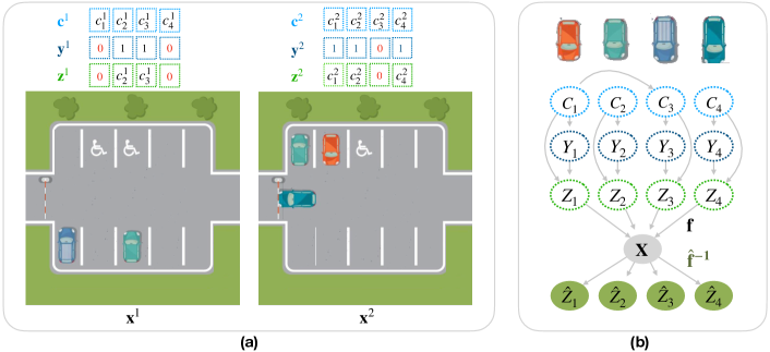
Figure 1: (a) Motivating example for the Unpaired Partial Observation setting: a stationary camera taking pictures of a car park. We consider $\mathbf{x}^{1}$ the image on day 1 and $\mathbf{x}^{2}$ the image on day 2. The latent causal variables $\mathbf{c}^{1}$ and $\mathbf{c}^{2}$ represent the positions of four cars on each day. In $\mathbf{x}^{1}$ only $Car2$ and $Car3$ are visible, while in $\mathbf{x}^{2}$ all cars except $Car3$ are visible. This is represented by the ones in the binary mask variables $\mathbf{y}^{1}$ and $\mathbf{y}^{2}$. The combination of the values of the latent causal variables $\mathbf{c}$ and the masks $\mathbf{y}$ are the masked causal variables $\mathbf{z}$, which used by the mixing function $\mathbf{f}$ to generate the images $\mathbf{x}$. (b) Causal model of the setting, the dotted line variables are not directly observed, but they are measured only through the observation $\mathbf{X}$. Our goal is to learn a representation $\hat{\mathbf{Z}}$ that identifies $\mathbf{Z}$ up to permutation and element-wise transformation.

We highlight the following contributions:

• We formalize the Unpaired Partial Observations setting for CRL, where each partial observation captures only a subset of causal variables and the observations are unpaired, i.e., we do not have simultaneous partial observations of the same state of the system.

• We introduce two theoretical results for identifying causal variables up to permutation and element-wise transformation under partial observability. Both results leverage a sparsity constraint. In particular, Thm. 3.1 proves identifiability for linear mixing function and without parametric assumptions on the underlying causal model. Thm. 3.4 proves identifiability for the piecewise linear mixing function, when the causal variables are Gaussian and we can group observations by their partial observability patterns.

• Finally, we propose two methods that implement these theoretical results and validate their effectiveness with experiments on simulated data and image benchmarks, e.g. Causal3DIdent (von Kügelgen et al., 2021), that we modify to test our partial observability setting.

2 Problem setting

In this section, we formalize the Unpaired Partial Observation setting, in which we have a set of high-dimensional observations that are functions only of instance-dependent subsets of the true underlying causal variables. This setting consists of four sets of random variables: the causal variables $\mathbf{C}$, the binary mask variables $\mathbf{Y}$ that represent if a variable is measured in a sample, the masked causal variables $\mathbf{Z}$ that combine the information from the causal variables and the masks, and the observations $\mathbf{X}$. Our goal is to recover the masked causal variables $\mathbf{Z}$ up to permutation and element-wise transformation, solely from the observations $\mathbf{X}$, despite the instance-dependent partial observability pattern. We show an example of a causal graph of the setting in Fig 1b and discuss each component in the following.

Causal variables $\mathbf{C}$. We define our latent causal variables as a random vector $\mathbf{C}=(C_{1},...,C_{n})$ that takes values in $\mathcal{C}=\mathcal{C}_{1}\times...\times\mathcal{C}_{n}\subseteq\mathbb{R}^{n}$, which is an open, simply connected latent space. The causal variables follow a distribution with density $p(\mathbf{C})$, which allows for causal relations between them. We assume that $p(\mathbf{c})\neq 0$ for all $\mathbf{c}\in\mathcal{C}$.

Mask variables $\mathbf{Y}$. We use a binary mask random variable $\mathbf{Y}=(Y_{1},\dots,Y_{n})$ with domain $\mathcal{Y}\subseteq\{0,1\}^{n}$ to represent the dynamic partial observability patterns, i.e., the causal variables that are measured in each of the samples. If $Y_{i}=1$ then we consider the variable $C_{i}$ measured, i.e. captured in the observation, otherwise it is considered unmeasured. We assume $\mathbf{Y}$ follows $p(\mathbf{Y})$. Further, we define the support index random set $\mathbf{S}$ as the index of non-zero components of $\mathbf{Y}$, i.e., $\mathbf{S}:=\{i\in[n]:Y_{i}\neq 0\}$. The support index set has a probability mass function $p(\mathbf{s})$ and support ${\mathcal{S}}$ defined as:

$$\mathbb{P}(\mathbf{s}):=\mathbb{P}\left(\bigwedge_{j\in\mathbf{s}}(\mathbf{Y}_{j}=1)\land\bigwedge_{j\not\in\mathbf{s}}(\mathbf{Y}_{j}=0)\right)\,\ \ \mathrm{and}\ \ \mathcal{S}:=\{\mathbf{s}\subseteq[n]\mid p(\mathbf{s})>0\}.$$

This definition allows us to model also dependences between the components of $\mathbf{Y}$ and masking behavior that depends on the values of the underlying causal variables.

Masked causal variables $\mathbf{Z}$. The masked causal variables $\mathbf{Z}=(Z_{1},...,Z_{n})\in\mathcal{Z}$ are a combination of the causal variables and the masks, and they are the latent inputs to the mixing function $\mathbf{f}$ that we are trying to recover. In particular, they are the Hadamard product of the causal variables with the binary mask variable, i.e., $\mathbf{Z}=\mathbf{Y}\odot\mathbf{C}$. This means that for sample $i\in[N]$ and any causal variable $j\in[n]$, if the mask value $y^{i}_{j}$ is $1$, then the causal variable $c^{i}_{j}$ is measured and $z^{i}_{j}$ is $c^{i}_{j}$. Instead, if $y^{i}_{j}=0$, then the causal variable is unmeasured and $z^{i}_{j}$ takes a fixed masked value $M_{j}$, which we will consider for simplicity to be $0$. Finally, we assume that for all $\mathbf{s}\in\mathcal{S}$, the probability measure $\mathbb{P}_{\mathbf{Z}_{\mathbf{s}}\mid\mathbf{S}=\mathbf{s}}$ has a density w.r.t. the Lebesgue measure on $\mathbb{R}^{|\mathbf{s}|}$.

Observations $\mathbf{X}$. We assume that observations $\mathbf{X}\in\mathcal{X}\subseteq\mathbb{R}^{d}$ are generated by mixing the masked causal variables $\mathbf{Z}$ with the same mixing function $\mathbf{f}:\mathcal{Z}\rightarrow\mathcal{X}$, i.e., $\mathbf{X}=\mathbf{f}(\mathbf{Z})$. We refer to partitions of observations with the same unknown partial observability pattern, i.e., with the same unknown value of $\mathbf{Y}=\mathbf{y}$, as groups, and we assume that each observation $\mathbf{x}^{i}$ for $i\in[N]$ is part of a group $g^{i}\in\mathcal{G}$.

Our goal is to identify the masked causal variables $\mathbf{Z}$ from a set of observations $\mathbf{X}$. In CRL we usually cannot recover the exact value of the latent variables, but we can only identify them up to some transformation. Our results guarantee that each ground truth variable is represented by a single estimated variable up to a linear transformation. Similar notions of identifiability were used in previous works (Comon, 1994; Khemakhem et al., 2020; Lachapelle et al., 2023).

Definition 2.1.

The ground truth representation vector $\mathbf{Z}$ is said to be identified up to permutation and element-wise linear transformation by a learned representation vector $\hat{\mathbf{Z}}$ when there exists a permutation matrix $\mathbf{P}$ and an invertible diagonal matrix $\mathbf{D}$ such that $\hat{\mathbf{Z}}=\mathbf{P}\mathbf{D}\mathbf{Z}$ almost surely.

To prove our results, we describe the sufficient support index variability, which was originally defined by Lachapelle et al. (2023) for sparse multitask learning for disentanglement.

Assumption 2.2.

(Sufficient support index variability (Lachapelle et al., 2023)) For all $i\in[n]$, we assume that the union of the support indices $\mathbf{s}$ that do not contain $i$ covers all of the other causal variables, or more formally:

$$\bigcup_{\mathbf{s}\in{\mathcal{S}}\mid i\notin\mathbf{s}}\mathbf{s}=[n]\setminus\{i\}\,.$$

This assumption avoids cases in which two variables are always missing at the same time, since then we would not be able to disentangle them from the observations.

3 Identifiability via a Sparsity Principle

In this section, we show how a simple sparsity constraint on the learned representations allows us to learn a disentangled representation of the ground truth variables. We first consider linear mixing functions and prove identifiability without any parametric assumption on the causal variables and while allowing for partial observability patterns that can depend on the value of the causal variables (Thm. 3.1). We then investigate if this sparsity principle can also identify variables for nonlinear mixing functions $\mathbf{f}$. This is not the case in general, as we show in Example 3.1.

Our linear result hinges on the existence of a function $\mathbf{g}$ such that the composition of $\mathbf{g}$ and $\mathbf{f}$ is affine. Based on this intuition, we consider piecewise linear mixing functions $\mathbf{f}$, since for Gaussian causal variables they can be composed with an appropriate $\mathbf{g}$ to obtain an affine function. In this setting, we prove that we can learn a disentangled representation of the latent variables (Def. 2.1) given that the masks are independent of the causal variables and given that we know the groups of the observations (Thm. 3.4).

3.1 Linear Mixing Function

We show that for linear mixing functions under a perfect reconstruction (Eq. 49), a simple sparsity constraint on the learned representation (Eq. 2) allows us to learn a disentangled representation of the ground truth latent variables.

Theorem 3.1 (Element-wise Identifiability for Linear $\mathbf{f}$).

Assume the observation $\mathbf{X}=\mathbf{f}(\mathbf{Z})$ follows the data-generating process in Sec. 2, where $\mathbf{f}:\mathcal{Z}\to\mathcal{X}$ is an injective linear function, and Ass. 2.2 holds. Let $\mathbf{g}:\mathcal{X}\rightarrow\mathbb{R}^{n}$ be an invertible linear function onto its image and let $\hat{\mathbf{f}}:\mathbb{R}^{n}\rightarrow\mathbb{R}^{d}$ be an invertible continuous function onto its image. If both of the following conditions hold,

$$\mathbb{E}\left\lVert\mathbf{X}-\hat{\mathbf{f}}(\mathbf{g}(\mathbf{X}))\right\rVert^{2}_{2}=0\,,\quad\text{and}$$ (1)

$$\mathbb{E}\left\lVert\mathbf{g}(\mathbf{X})\right\rVert_{0}\leq\mathbb{E}\left\lVert\mathbf{Z}\right\rVert_{0},$$ (2)

then $\mathbf{Z}$ is identified by $\hat{\mathbf{f}}^{-1}(\mathbf{X})$ up to a permutation and element-wise linear transformations (Def. 2.1), i.e., $\hat{\mathbf{f}}^{-1}\circ\mathbf{f}$ is a permutation composed with element-wise invertible linear transformations on $\mathcal{Z}$.

We provide a proof in App. A.1 and now give an intuitive explanation for why it holds. The zero reconstruction loss ensures that no information is lost in the encoding $\mathbf{g}(\mathbf{X})$, which implies that $\mathbf{g}(\mathbf{X})$ is not sparser than $\mathbf{Z}$. Hence, incorporating Eq. (2) as a constraint or regularization term in our methods enables our estimators to match the sparsity of the ground truth variables, which breaks indeterminacies due to rotations of the latent space.

The idea of using a sparsity constraint or regularization is similar to previous work (Lachapelle et al., 2022) in the context of sparse multitask learning. In this paper we leverage these ideas in the distinct setting of partial observability. Interestingly, this result does not require the invertibility of the mixing function $\mathbf{f}$, as most other results in CRL. Notably, it also does not require any parametric assumptions on the distribution of $\mathbf{Z}$, thus allowing for causal relations or other statistical dependencies among the latent variables. Finally, this result also allows for mask variables that potentially depend on the values of the latent causal variables.

3.2 Is sparsity enough for identification for nonlinear $\mathbf{f}$?

Since linearity of $\mathbf{f}$ is a strong assumption that may not hold in many applications, an obvious question is whether we can extend this result to nonlinear mixing functions. Unfortunately, this is not the case without making further assumptions, as demonstrated by the following example.

Example 3.1.

Consider $\mathbf{C}\sim\mathcal{N}(0,\mathbf{I}_{2})$, where $\mathbf{I}_{2}$ is the identity matrix.

Assume an independent mask $\mathbf{Y}$ with distribution $p(\mathbf{Y}=\mathbf{y})=1/4$ for any $\mathbf{y}\in\{0,1\}^{2}$, satisfying Ass. 3.3. Let the nonlinear mixing function $\mathbf{f}:\mathbb{R}^{2}\rightarrow\mathbb{R}^{2}$ be

$$\mathbf{f}(\mathbf{z}):=\sinh(\mathbf{R}_{\frac{\pi}{4}}\mathbf{z})+\sinh(\mathbf{R}_{-\frac{\pi}{4}}\mathbf{z})\,,$$ (3)

where $\mathbf{R}_{\theta}$ is a rotation matrix. Consider $\hat{\mathbf{f}}$ and $\mathbf{g}$ to be the identity function, which trivially satisfy Eq. 49, since $\hat{\mathbf{f}}\circ\mathbf{g}(\mathbf{X})=\mathbf{X}$. We show in Appendix B that $\mathbf{g}$ satisfies the sparsity constraint (Eq. 2). However, despite satisfying all requirements of Thm 3.1 except for the linearity of $\mathbf{f}$, we can show that each component of $\hat{\mathbf{f}}^{-1}\circ\mathbf{f}=\mathbf{f}$ depends on both components of $\mathbf{z}$; or in other words, the learned representation does not identify $\mathbf{Z}$ up to permutation and element-wise transformations. We refer to App. B for details.

3.3 Piecewise Linear Mixing Function

In light of Example 3.1, we consider the role of linearity in Thm. 3.1. We notice that it is a sufficient condition for ensuring that there exists a $\mathbf{g}$ such that $\mathbf{g}\circ\mathbf{f}$ is affine on $\mathcal{Z}$. We then consider the question: even if $\mathbf{f}$ is not affine itself, can we consider a restricted class of $\mathbf{f}$ and latent variables $\mathbf{Z}$ such that the composition of $\mathbf{f}$ and an appropriate $\mathbf{g}$ is affine? As a first step we consider a piecewise linear $\mathbf{f}$ and assume that the causal variables are Gaussian and that the masks are independent from the causal variables.

Assumption 3.2.

We assume $\mathbf{C}$ follows a non-degenerate multivariate normal distribution, i.e. $\mathbf{C}\sim N(\bm{\mu},\bm{\Sigma})$, where $\bm{\mu}\in\mathbb{R}^{n}$ and $\bm{\Sigma}\in\mathbb{R}^{n\times n}$ is a positive definite matrix.

Assumption 3.3.

We assume $\mathbf{C}$ and $\mathbf{Y}$ are independent from each other, i.e. the partial observability pattern does not depend on the values of the causal variables.

These assumptions represent a classical linear Gaussian Structural Causal Model setting for the causal variables and a missing-at-random assumption in terms of which variables are measured in the observation. On the other hand, in our setting, we do not directly observe the causal variables or the masks, but we only observe them mixed in an observation.

Under these assumptions, the conditional distribution of the masked causal variables $\mathbf{Z}$ given the binary mask vector $\mathbf{Y}$ is defined as a multivariate normal distribution:

$$\mathbf{Z}~{}|~{}\mathbf{Y} \sim N(\bm{\mu}_{\mathbf{Y}},\bm{\Sigma}_{\mathbf{Y}})$$

$$\text{where }\bm{\mu}_{\mathbf{Y}}=(\mu_{1}Y_{1},\dots ,\mu_{n}Y_{n}),\quad\bm{\Sigma}_{\mathbf{Y}(ij)}=\bm{\Sigma}_{ij}Y_{i}Y_{j}$$

This distribution is a degenerate multivariate normal (De-MVN), i.e., a normal with a singular covariance matrix, if at least one of the causal variables is masked by $\mathbf{Y}$.

Intuitively, we can leverage the Gaussianity of $\mathbf{Z}|\mathbf{Y}$ to enforce that the reconstructed $\hat{\mathbf{Z}}|\mathbf{Y}=\mathbf{g}(\mathbf{X})$ is also Gaussian. We now show that this allows us to identify the latent factors $\mathbf{Z}$ through our sparsity constraint on the learned representations (Eq. 5), given that we are able to partition the data according to the unknown value of $\mathbf{Y}=\mathbf{y}$, or in other words, given that we know the group $g_{i}$ for each observation $\mathbf{x}_{i}$ for $i\in[N]$. The rationale of this requirement is that we do not need to know the value of the latent mask $\mathbf{Y}$, but we do need to be able to separate observations that are generated by different distributions of $\mathbf{Z}$, so we can effectively enforce the Gaussianity constraint (Eq. 6).

Theorem 3.4 (Element-wise Identifiability for Piecewise Linear $\mathbf{f}$).

Assume the observation $\mathbf{X}$ follows the data-generating process in Sec 2, Ass. 2.2, 3.2 and 3.3 hold and $\mathbf{f}:\mathcal{Z}\to\mathcal{X}$ is an injective continuous piecewise linear function. Let $\mathbf{g}:\mathcal{X}\rightarrow\mathbb{R}^{n}$ be a continuous invertible piecewise linear function and let $\hat{\mathbf{f}}:\mathbb{R}^{n}\rightarrow\mathbb{R}^{d}$ be a continuous invertible piecewise linear function onto its image. If all following conditions hold:

$$\mathbb{E}\left\lVert\mathbf{X}-\hat{\mathbf{f}}(\mathbf{g}(\mathbf{X}))\right\rVert^{2}_{2}=0\,,$$ (4)

$$\mathbb{E}\left\lVert\mathbf{g}(\mathbf{X})\right\rVert_{0}\leq\mathbb{E}\left\lVert\mathbf{Z}\right\rVert_{0}\text{ and }$$ (5)

$$\mathbf{g}(\mathbf{X})~{}|~{}(\mathbf{Y}=\mathbf{y})\sim N(\bm{\mu}_{\mathbf{y}},\bm{\Sigma}_{\mathbf{y}})\qquad\forall\mathbf{y}\in\mathcal{Y},$$ (6)

for some $\bm{\mu}_{\mathbf{y}}\in\mathbb{R}^{n},\bm{\Sigma}_{\mathbf{y}}\in\mathbb{R}^{n\times n}$, then $\mathbf{Z}$ is identified by $\hat{\mathbf{f}}^{-1}(\mathbf{X})$, i.e., $\hat{\mathbf{f}}^{-1}\circ\mathbf{f}$ is a permutation composed with element-wise invertible linear transformations (Def. 2.1).

We provide the complete proof in App. A.2. We first provide some results for a weaker notion of identifiability: identifiability up to affine transformations (Def. A.4). To this end, we first extend a theorem by Kivva et al. (2022) from the case of non-degenerate to potentially degenerate multivariate normal variables (Thm. A.5). Such variables are crucial in our setting because partial observability potentially introduces degenerate cases. The crux of our proof involves handling the case of degenerate variables that do not have probability density. We then show that given the information of the binary mask $\mathbf{Y}$, we can identify the latent factors $\mathbf{Z}$ up to an affine function $\mathbf{h}_{\mathbf{Y}}$ (Lemma A.10). We then show that all of these affine functions can be represented by a single affine function $\mathbf{v}:=\hat{\mathbf{f}}^{-1}(\mathbf{f}(\mathbf{Z}))$ defined on $\mathcal{Z}$.

Compared to linear case in Thm. 3.1, the additional constraint in this case is Gaussianity on both $\mathbf{Z}|\mathbf{Y}$ and the estimator $\mathbf{g}(\mathbf{X})|\mathbf{Y}$. This ensures that the composition of two piecewise linear functions $\mathbf{g}$ and $\mathbf{f}$ remains affine on $\mathcal{Z}$, extending the results from linear $\mathbf{f}$ to piecewise linear $\mathbf{f}$.

Non-zero mask values. Our theoretical analysis assumes that we mask the unmeasured latent variables with a mask value of $0$, i.e. when $\mathbf{y}^{i}=0$ for $i\in[N]$, we set $\mathbf{z}_{i}=0$. One can wonder whether allowing to set $\mathbf{z}^{i}=\mathbf{M}$ when $\mathbf{y}_{i}=0$ for some potentially nonzero constant vector $\mathbf{M}$ would make the model more expressive. It turns out that this is not the case, since the decoder $\mathbf{f}$ can always shift $\mathbf{Z}$ in arbitrary ways, making the specific value of $\mathbf{M}$ irrelevant.

4 Implementation

We implement our two theoretical results asconstrained optimization problems in Cooper  (Gallego-Posada and Ramirez, 2022). We approximate the sparsity constraint, i.e. Eq. 2 in Thm. 3.1 and Eq. 5 in Thm. 3.4, by replacing the $L_{0}$ norm with $L_{1}$ norm, which is differentiable except at zero. In practice, the $L_{1}$ norm of the ground truth variables $\mathbf{Z}$ is unknown, so we instead set a hyperparameter $\epsilon$ for the sparsity constraint $\mathbb{E}\left\lVert\mathbf{g}(\mathbf{X})\right\rVert_{1}\leq\epsilon$. In our experiments, we use $\epsilon=0.01$ or $0.001$, details are provided in App. D.2.

For linear $\mathbf{f}$, we can reconstruct the latent variables directly from a dataset of observations $\{\mathbf{x}^{i}\}_{i\in[N]}$ by minimizing the reconstruction error and adding the sparsity constraint (Thm 3.1). For piecewise linear $\mathbf{f}$, Thm. 3.4 requires that we know how to partition the data with the same partial observability, i.e., we have information about the group of each observation. At test time, we have already learned $\mathbf{g}$, so we can instead use only the observations without the group information. To encourage the Gaussianity condition on $\mathbf{g}(\mathbf{X})|\mathbf{Y}=\mathbf{y}$ (Eq. 6) in Thm. 3.4, we add two regularization terms that push the estimated skewness of each latent variable in each group to be 0 and the estimated kurtosis to be 3, which are the values of these moments in the Gaussian distribution. We learn the encoder $\mathbf{g}_{\psi}$ and the decoder $\hat{\mathbf{f}}_{\theta}$ by solving the following optimization problem:

$$\min_{(\theta,\psi)} \frac{1}{N}\sum_{i\in[N]}\left\lVert\mathbf{x}^{i}-\hat{\mathbf{f}}_{\theta}(\mathbf{g}_{\psi}(\mathbf{x}^{i}))\right\rVert^{2}_{2}+\sum_{g\in\mathcal{G}}\Big{(}\left|\mathrm{\widehat{skew}}_{g}\left(\mathbf{g}_{\psi}(\mathbf{x})\right)\right|+\left|\mathrm{\widehat{kurt}}_{g}\left(\mathbf{g}_{\psi}(\mathbf{x})\right)-3\right|\Big{)}$$

$$\text{subject to: \quad}\frac{1}{nN}\sum_{i\in[N]}\left\lVert\mathbf{g}_{\psi}(\mathbf{x}^{i})\right\rVert_{1}\leq\epsilon,$$ (7)

where $\mathrm{\widehat{skew}}_{g}\left(\mathbf{g}_{\psi}(\mathbf{x})\right)$ and $\mathrm{\widehat{kurt}}_{g}\left(\mathbf{g}_{\psi}(\mathbf{x})\right)$ are the estimated skewness and estimated kurtosis for group $g\in\mathcal{G}$. We solve both problems with the extra-gradient version of Adam Gidel et al. (2018). We provide all details in App. D.

5 Experimental Results

We perform three sets of experiments, one with numerical data in Sec. 5.1 and two with image datasets, a dataset with multiple balls in Sec. 5.2 and PartialCausal3DIdent, a partially observable version of Causal3DIdent (von Kügelgen et al., 2021) in Sec. 5.3. Following previous work (Hyvarinen et al., 2019; Khemakhem et al., 2020), we report the mean coefficient of determination (MCC) to assess that the learned representations match the ground truth up to a permutation and element-wise linear transformations. This metric is based on the Pearson correlation matrix $\mathrm{Corr}^{n\times n}$ between the learned representations $\hat{\mathbf{Z}}=\mathbf{g}(\mathbf{X})$ and ground truth masked causal variables $\mathbf{Z}$. Since our results are up to permutation, we compute the MCC on the permutation $\pi$ that maximizes the average of $|\mathrm{Corr}_{i,\pi(i)}|$ for each index of a ground truth variable $i\in[n]$, i.e. MCC=$\frac{1}{n}\max_{\pi\in perm([n])}\sum_{i=1}^{n}|\mathrm{Corr}_{i,\pi(i)}|$. We denote the correlation matrix with the permutation $\pi$ as $\mathrm{Corr}^{n\times n}_{\pi}$.

5.1 Numerical Experiments

We generate numerical data following Sec. 2. We consider varying the partial observability patterns, the underlying causal model and the type of mixing function $\mathbf{f}$. For the encoder $\mathbf{g}$ and the decoder $\hat{\mathbf{f}}$, we use 7-layer MLPs with LeakyReLU layers with $[10,50,50,50,50,10]\times n$ units per layer, where $n$ is the number of causal variables, and apply batch normalization to control the norm of $\mathbf{g}(\mathbf{X})$. In each setup, we average over 3 random seeds.

We experiment with different ratios of measured variables $\rho=\{1\textsc{var},50\%,75\%\}$, where $1\textsc{var}$ is one measured variable, while $50\%$ and $75\%$ are the percentages of measured variables in each sample. Based on each $\rho$ we predefine a set of $K$ masks $\mathbf{Y}$ that satisfies Ass. 2.2. As discussed in Sec. 3, while the theoretical results assume a mask value of $\mathbf{M}=\mathbf{0}$, the specific value used is inconsequential from the theoretical point of view. On the other hand, the optimization procedure improves for mask values that are out of distribution w.r.t. the unmasked distribution of each variable, since it is then easier to recover which variables are masked in each group. We investigate different masks values and consider $\mathbf{M}=\bm{\mu}+\delta\cdot\sigma$, where $\bm{\mu},\sigma\in\mathbb{R}^{n}$ are the mean and standard deviation of $\mathbf{Z}$ and $\delta\in\{0,2,3,5,10\}$.

We consider $n=\{3,5,10,20,40\}$ causal variables $\mathbf{C}$. In each experiment, we generate a random directed acyclic graph $\mathcal{D}$ from a random graph Erdös-Rényi (ER)-$k$ model, where $k\in\{0,1,2,3\}$ and ER-$k$ is a graph with $n\cdot k$ edges. In particular, ER-0 implies independent $\mathbf{C}$ and therefore $\mathbf{Z}$. Based on $\mathcal{D}$, we consider three types of structure causal models (SCM): i) a linear Gaussian SCM where edge weights are sampled uniformly from $[-2,-0.5]\cup[0.5,2]$ and we use standard Gaussian noises; ii) a linear exponential SCM, where we have a similar setup, but with exponential noises with scale 1; iii) a nonlinear SCM, where we simulate a nonlinear function with a one linear layer followed by a sigmoid activation plus a fully connected layer with $2n$ hidden units, where edge weights are sampled uniformly from $[-2,-0.5]\cup[0.5,2]$ and we use standard Gaussian noises.

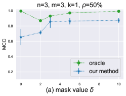
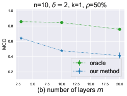
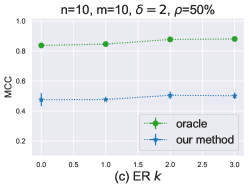
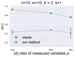
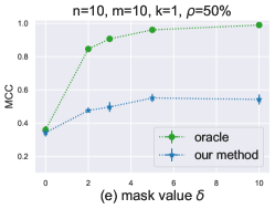
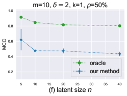
Figure 2: Results for different parameters in the piecewise linear numerical experiments. Our method implements Eq. 4 based on the group information. The oracle method implements the same loss, but with as additional information the mask $\mathbf{y}_{i}$, which it uses to assign a low variance to the masked variables in each sample for the skewness and kurtosis regularization terms. This method showcases the potential of our theoretical results with a stronger Gaussianity constraint.

.

Table 1: Results for the numerical experiments for linear mixing functions with $\delta=0$. The bold font indicates which parameters are varying in each block of rows.

$n$	$k$	SCM	$\rho$	MCC
5	1	Lin. Gauss	50 %	0.995$\pm$0.000
10	1	Lin. Gauss	50 %	0.970$\pm$0.046
20	1	Lin. Gauss	50 %	0.849$\pm$0.022
40	1	Lin. Gauss	50 %	0.492$\pm$0.030
10	0	Indep. Gauss	50 %	0.997$\pm$0.001
10	1	Lin. Gauss	50 %	0.970$\pm$0.046
10	2	Lin. Gauss	50 %	0.647$\pm$0.099
10	3	Lin. Gauss	50 %	0.243$\pm$0.319
10	0	Indep. Exp	50 %	0.997$\pm$0.001
10	1	Lin. Exp	50 %	0.996$\pm$0.001
10	2	Lin. Exp	50 %	0.671$\pm$0.021
10	3	Lin. Exp	50 %	0.294$\pm$0.364
10	1	Nonlinear	50 %	0.957$\pm$0.017
10	2	Nonlinear	50 %	0.742$\pm$0.076
10	3	Nonlinear	50 %	0.643 $\pm$0.074
10	1	Lin. Gauss	1var	0.996 $\pm$0.000
10	1	Lin. Gauss	50 %	0.970$\pm$0.046
10	1	Lin. Gauss	75 %	0.756 $\pm$0.032

Results for linear mixing function (Thm. 3.1). We use a fully connected layer to model the linear mixing function $\mathbf{f}$. We show the performance, measured in the average MCC over three random seeds in table 1. In the first four rows, we investigate how the number of the latent causal variables influences the performance for a linear Gaussian SCM with an average degree $k=1$ and a ratio of measured variables $\rho=50\%$. In this case, the method achieves excellent performances for smaller $n$, but these degrade as $n$ increases. In the second group of rows, we consider the effect of $k$, the average degree in the causal graph in the linear Gaussian case for $n=10$ causal variables and $\rho=50\%$. Also in this case, the performances are excellent for low $k$, including $k=0$ which represents independent variables, but they degrade with higher $k$. The third and fourth group of rows show how the performance varies for different $k$ for the linear exponential and nonlinear SCM, showing a similar performance. Finally, we show the results for varying ratio of measured variables $\rho$, showing a small degradation when we measure more variables at the same time. Intuitively, measuring a smaller number of variables for each sample is the easier setting for disentangling them from the observations.

Results for piecewise linear mixing function (Thm. 3.4). For the piecewise linear $\mathbf{f}$, we use a $m=\{3,10,20\}$-hidden-layer MLP with $m-1$ LeakyReLU ($\alpha=0.2$) activation functions and a final linear layer, to model the piecewise linear mixing function. The number for layers $m$ in the $\mathbf{f}$ mixing function is a proxy for the complexity of the function $\mathbf{f}$, a linear function has $m=0$, while the higher the $m$ the higher the non-linearity. Following (Lachapelle et al., 2022), the weight matrices are sampled from a standard Gaussian distribution and are orthogonalized by their columns to ensure $\mathbf{f}$ is injective. In this setting, we evaluate with a linear Gaussian SCM, since this satisfies Ass. 3.2 in Thm. 3.4.

We start by showing results in Fig. 2a for the simple case of number of causal variables $n=3$ and number of layers $m=3$. Through optimization of Eq. (4), our approach achieves good performances in these simple scenarios. However, in more complex cases, e.g. more latent variables or more complicated $\mathbf{f}$, there is a decline in performance, as shown in Fig. 2b-f. We hypothesize that the reason for this drop is that the estimated skewness and kurtosis cannot guarantee Gaussianity, which is crucial to ensure identifiability in Thm. 3.4. We show that this is empirically the case for $n=5$ in Fig. 5 in App. D.3. We attribute this issue to the per-group sample variance used to calculate both sample skewness and kurtosis. We test this assumption and potential of our theoretical results, by comparing with an oracle that has access to the masks $\mathbf{y}^{i}$ for each observation $\mathbf{x}^{i}$. This information is used to set the group sample variance to a low value for the masked variables in each group. As shown in Fig. 2b-f this is effective in improving the performances of our sparsity constraint.

We test the performance of our method and the oracle for various parameters in Fig. 2. In particular, we see in Fig. 2a and Fig. 2e that when the distance $\delta$ between masked and unmasked variables increases, it enables a more distinct separation of $\mathbf{Z}$, providing better identification results. Similar to the linear case, we see that an increase in complexity, e.g., in the number of causal variable $n$, as shown in Fig. 2f, or the number of layers $m$, as shown in Fig. 2b, lowers the performance. Similarly, as shown in Fig. 2d, the performance drops when the ratio of measured variables $\rho$ increases. Interestingly, the average degree of the causal graph $k$ does not have an impact, as shown in Fig. 2c. We provide more results and visualizations in App. E.1.

5.2 Image dataset: Multiple Balls

We create a new image dataset in which we render in a 2D space $b$ moving balls, as shown in Fig. 16 in App. E.2. Our latent causal variables are the $(x,y)$ position of each ball $\mathbf{b}$, which we model as Gaussian. We consider two settings: i) a missing ball setting in which the balls can only move along the $x$-axis and they can move out of view; ii) a masked position setting in which the balls can move freely inside the frame and each of their coordinates can be masked by being set to an unknown, but fixed, $\mathbf{M}$ value. The missing ball setting represents the intuitive setting for partial observability, i.e. when an object is out of the frame or occluded. While we model each object with two causal variables, its $x$ and $y$ coordinates, our methods do not allow that masks for two variables are deterministically related (Ass. 2.2). Thus, we constrain the balls to move only on the $x$-axis, which we then identify from the observations. In order to test also the identifiability of each variable of the same object, we devise the masked position setting. In this setting, we can still use our method with a non-zero mask value for each variable, which in this case represents a specific value for one of the $x$ or $y$ coordinates of the ball. We generate datasets for both settings by varying the number of balls $b=2,5,8$. We use a predefined set of $K$ masks $\mathbf{y}$ that satisfies Ass. 2.2. For the missing ball setting, we generate the $x$-coordinates of each ball from a truncated normal distribution $\mathcal{N}(0.5,0.1^{2})$ with bounds $(0.1,0.9)$. For the masked position setting, we generate the $x$ and $y$-coordinates of each ball $i\in[b]$ independently from a truncated 2-dimensional normal distribution $\mathcal{N}(\bm{\mu}_{i},\bm{\Sigma}_{i})$ with bounds $(0.1,0.9)^{2}$, where $\bm{\mu}_{i}\sim Unif(0.4,0.6)^{2}$, and $\bm{\Sigma}_{i}=((0.01,0.005)(0.005,0.01))$ for all groups. For both settings, we generate the masked causal variables as $(\mathbf{Z}_{k})^{K}_{k=1}=\mathbf{y}\cdot\mathbf{C}+(1-\mathbf{y})\cdot\mathbf{M}\in\mathbb{R}^{K\times n}$, where $\mathbf{M}=\mathbf{0}$ for the missed ball setting, and $\mathbf{M}=\bm{\mu}_{i}+\delta\cdot\sigma_{i}$ for the masked position setting. Instead of a fixed-size training dataset, we generate images online until convergence. We provide more details in App. E.2.

Table 2: Results for the two settings in the multiple balls dataset.

$b$	MCC Missing	MCC Masked
2	0.963$\pm$0.012	0.946$\pm$0.005
5	0.950$\pm$0.011	0.939$\pm$0.003
8	0.928$\pm$0.004	0.901$\pm$0.002

As illustrated in Table 2, while the MCC decreases with an increase in the number of balls $b$, all MCCs remain above $0.90$. The results are consistently higher in the missing ball setting, where there are $b$ variables to reconstruct, while in the masked position setting there are $2b$. Additionally, in the masked position setting, we have dependence between the $x$ and $y$ coordinates, which can make the problem more challenging.

5.3 Image dataset: PartialCausal3DIdent

We explore the capability of our method on a partial observability version of Causal3DIdent (von Kügelgen et al., 2021) that we create. Causal3DIdent collects images of 7 object classes rendered from 10 causal variables, including object color, object positions, spotlight positions, etc. Each latent variable is rescaled into an interval of $[-1,1]$. The mixing function, i.e., the rendering process, is not piecewise linear (which violates the assumption in Thm. 3.4). We still evaluate our piecewise linear method, following the intuition that non-linear functions can be approximated up to an arbitrary precision by an adequate number of linear pieces.

Since Causal3DIdent is fully observable, we sample from it to create PartialCausal3DIdent, a dataset in which some of the latent variables are masked to a predefined value. For each datum, we sample a latent vector $\mathbf{C}\sim\mathcal{N}(0,\sigma^{2}\mathbf{I})$ of $n=10$ independent causal variables. We apply the set of $K$ predefined masks $\mathbf{y}\in\{0,1\}^{K\times n}$ to get a set of masked latent variables $(\mathbf{Z}_{k})^{K}_{k=1}=\mathbf{y}\cdot\mathbf{C}+(1-\mathbf{y})\cdot\mathbf{M}\in\mathbb{R}^{K\times n}$. We define the masked value as the maximum of the support area (which is 1 for all latents). The ratio of the measured variables $\rho$ varies from 10% (only one latent is measured) to 100% (all latents are measured). The average $\rho$ is set to $50\%$. After obtaining the masked latent variables, we retrieve $K$ corresponding images from the dataset, based on the index searching scheme provided by von Kügelgen et al. (2021). We evaluate our method separately on each object class in PartialCausal3DIdent and show the results in Table 3. Although the performance fluctuates slightly across classes, our method achieves a high MCC over $80\%$ for all classes, which verifies that our approach is empirically applicable even on highly nonlinear high dimensional data. We provide all details and ablation studies on $\delta$ in App. E.3.

Table 3: MCC on PartialCausal3DIdent over each object class, with masking distance $\delta=10$ for all latent variables.

Object class id	0	1	2	3
MCC (mean $\pm$ std)	$0.842\pm 0.018$	$0.804\pm 0.023$	$0.828\pm 0.014$	$0.820\pm 0.009$
Object class id	4	5	6	avg. mean
MCC (mean $\pm$ std)	$0.837\pm 0.020$	$0.821\pm 0.033$	$0.858\pm 0.005$	$0.832\pm 0.016$

6 Related work

We summarize the most related works in this section and present an extended version of the related work in App. C. Most closely related to our work are recent identifiability studies, which also explicitly learn causal representations in a partially observable setting. Yao et al. (2023) consider learning from tuples of simultaneously observed views, which depend on different fixed (potentially overlapping) subsets of latents with modality-specific mixing functions, and prove identifiability results for different blocks of shared content variables (von Kügelgen et al., 2021). Compared to our setting, such paired multi-view data may be harder to obtain. Sturma et al. (2023) study an unpaired, multi-domain setup, in which observations from each domain depend on a different fixed subset of latents, and show identifiability of the causal representation and graph in the fully linear case. This setting resembles our results for the piecewise linear case in Thm. 3.4, where we assume we have the group information for each observation, which can be seen as a single domain. On the other hand, for the linear case in Thm. 3.1, we do not need the group information, hence we also allow for mixtures of data from multiple domains.

Other works have also explored the piecewise linear setting for identifiability, including with the assumption of Gaussian causal variables. In particular, Thm. 3.4 resembles one of the identifiability results from Kivva et al. (2022) which assumes $\mathbf{Z}$ is a mixture of non-degenerate Gaussians and $\mathbf{f}$ is a piecewise linear function. In Thm. 3.4, $\mathbf{Z}$ is also a mixture of Gaussians, where the “cluster index” corresponds to $\mathbf{Y}$. However, this mixture contains components which are degenerate, in the sense that their covariances might be singular (this occur when $\mathbf{Y}_{i}=0$ for some $i$). This prevents us from applying the result of Kivva et al. (2022) directly to our setting. On the other hand, although we allow for degenerate components, our result assumes knowledge of the groups $g$, unlike Kivva et al. (2022).

Prior work has also leveraged sparsity in representation learning, for example via a Spike and Slab prior (Tonolini et al., 2020; Moran et al., 2022), or by relating the learnt representation to multiple tasks, each depending only on a small subset of latents (Lachapelle et al., 2023; Fumero et al., 2023). Most closely related to ours is work by Lachapelle et al. (2022, 2024), who have proposed a sparsity principle for identifiable CRL in interventional and temporal settings, motivated by the sparse mechanism shift hypothesis (Schölkopf et al., 2021; Perry et al., 2022).

7 Conclusions and Limitations

In this work, we focused on learning causal representations in the unpaired partial observability setting, i.e., when only an instance-dependent subset of causal variables are captured in the measurements. We first proved the identifiability with linear mixing functions $\mathbf{f}$ under a sparsity constraint. We then presented an example to illustrate why extending the results to nonlinear $\mathbf{f}$ is not possible without additional assumptions. We proved identifiability when $\mathbf{f}$ is piecewise linear, both the causal variables and the learned representations are Gaussian, and we know the group of each sample.

While our experiments validate our theoretical results, there are still several limitations. From the theoretical point of view, knowing the group of each sample might not always be possible, so extending our results beyond this limitation is an exciting research direction. Additionally, piecewise linear functions are still a limited class and there might be other classes of nonlinear functions for which our identifiability results could be extended. Finally, our Gaussianity constraint is empirically difficult to satisfy, as shown by the gap between the performances of our method and the oracle. This warrants further investigation in other ways to encourage Gaussianity of the learned representations.

Appendix A Proofs

A.1 Proof of the results for linear mixing functions (Theorem 3.1)

We first introduce the definition of dependent inputs, which intuitively is the set of variables on which a reconstruction of a given variable depends.

Definition A.1.

Let $\mathbf{v}:\mathcal{Z}\rightarrow\mathbb{R}^{n}$ be a function with variables $\mathbf{z}=(z_{1},...,z_{n})\in\mathcal{Z}$.

For all $i\in[n]$ consider $N_{i}$ to be the set of all variables on which $\mathbf{v}_{i}$ depends, which we will call dependent inputs. Formally, we define the set of dependent inputs $N_{i}\subseteq[n]$ as

$$N_{i}:=\{j\in[n]\mid\exists(z_{j},\mathbf{z}^{0}_{-j}),(z^{\prime}_{j},\mathbf{z}^{0}_{-j})\in\mathcal{Z}\text{ where }z_{j}\neq z^{\prime}_{j}\text{ s.t. }\mathbf{v}_{i}(\mathbf{z}^{0}_{-j},z_{j})\neq\mathbf{v}_{i}(\mathbf{z}^{0}_{-j},z^{\prime}_{j})\}\,,$$ (8)

where $\mathbf{z}^{0}_{-j}$ is any $n-1$ dimensional vector that represents all of the components of a vector $\mathbf{z}\in\mathcal{Z}$ except for the index $j$.

This definition intuitively represents the indices of $\mathbf{z}$ for which the function $\mathbf{v}_{i}$ is not constant, or in other words, the inputs on which $\mathbf{v}_{i}$ depends. Note that if there is only one $z_{j}$ such that $(z_{j},\mathbf{z}^{0}_{-j})\in\mathcal{Z}$ for an appropriate $\mathbf{z}^{0}_{-j}$, then any function defined on $\mathcal{Z}$ is constant for that index, and hence $N_{i}$ does not contain $j$.

We now show a lemma that we will use to prove the theorem showing that for any diffeomorphism and any variable, there always exists a permutation that ensures that a variable is in the set of its dependent inputs. Intuitively, this ensures that for all variables, there always exists a permutation, such that the reconstruction of a given variable depends on the variable itself.

Lemma A.2 (Existence of permutation $\pi$ s.t. $i\in N_{\pi(i)}$).

Let $\mathbf{v}:\mathcal{Z}\rightarrow\mathbb{R}^{n}$ be a diffeomorphism onto its image with variables $\mathbf{z}=(z_{1},...,z_{n})\in\mathcal{Z}$. Assume there exists a point $\mathbf{z}^{0}\in\mathcal{Z}$ and a value $\epsilon>0$, such that $\forall i\in[n]$, $\mathbf{e}_{i}\odot[-\epsilon,\epsilon)^{n}+\mathbf{z}^{0}\subset\mathcal{Z}$, where $\mathbf{e}_{i}$ is the standard basis for space $\mathbb{R}^{n}$ for the $i$-th dimension, i.e. a $n$-dimensional vector in which all dimensions except $i$ are 0, and the $i$-th dimension is 1. Then there exists a permutation $\pi:[n]\rightarrow[n]$ such that $i\in N_{\pi(i)}$ for all $i$, where $N_{i}$ is defined as in Def. A.1.

Proof.

Since $\mathbf{v}$ is a diffeomorphism, its Jacobian $D\mathbf{v}=\{\frac{\partial\mathbf{v}_{i}}{\partial z_{j}}\}_{i,j\in[n]}$ is invertible everywhere, so it is invertible at $\mathbf{z}^{0}\in\mathcal{Z}$. Since $D\mathbf{v}(\mathbf{z}^{0})$ is invertible, we have that its determinant is non-zero, i.e.

$$\det(D\mathbf{v}(\mathbf{z}^{0})):=\sum_{\pi\in\mathfrak{S}_{n}}\text{sign}(\pi)\prod_{i=1}^{n}D\mathbf{v}(\mathbf{z}^{0})_{\pi(i),i}\neq 0\,,$$ (9)

where $\mathfrak{S}_{n}$ is the set of $n$-permutations. This equation implies that at least one term of the sum is non-zero, and that for that term, all of the terms in the product are non-zero, meaning:

$$\exists\pi\in\mathfrak{S}_{n},\forall i\in[n],D\mathbf{v}(\mathbf{z}^{0})_{\pi(i),i}\neq 0\;.$$ (10)

This means that, for all $i\in[n]$, $\frac{\partial\mathbf{v}_{\pi(i)}}{\partial z_{i}}(\mathbf{z}^{0})\not=0$, which implies that $\mathbf{v}_{\pi(i)}$ is not constant for $z_{i}$ in $\mathbf{z}^{0}$. Then by definition of $N_{i}$ in Def. A.1, $i\in N_{\pi(i)}$.

∎

As an intermediate step, we first prove an important lemma that shows that by enforcing sparsity of the transformed variables, the corresponding transformation is an element-wise linear function. Intuitively, these transformed variables will be the reconstructed masked latent variables $\mathbf{Z}$.

Lemma A.3 (Element-wise Identifiability for Linear Transformation).

Assume that the masked latent variables $\mathbf{Z}$ with support $\mathcal{Z}$ follow the data generating process in Sec. 2 and Ass. 2.2 holds. Let the function $\mathbf{v}:\mathcal{Z}\rightarrow\mathbb{R}^{n}$ be invertible and linear on $\mathcal{Z}$, and

$$\mathbb{E}\left\lVert\mathbf{v}(\mathbf{Z})\right\rVert_{0} \leq\mathbb{E}\left\lVert\mathbf{Z}\right\rVert_{0}.$$ (11)

Then $\mathbf{v}$ is a permutation composed with an element-wise invertible linear transformation on $\mathcal{Z}$.

Proof.

We reuse the definition of the support indices $\mathbf{S}:=\{i\in[n]:Z_{i}\neq 0\}$ and analyze each side of inequality (11), starting with its right-hand side.

$$\mathbb{E}||\mathbf{Z}||_{0} =\mathbb{E}\sum^{n}_{i=1}\mathbbm{1}(\mathbf{Z}_{i}\not=0)$$ (12)

$$=\sum_{\mathbf{s}\in\mathcal{S}}p(\mathbf{s})\mathbb{E}\left[\sum^{n}_{i=1}\mathbbm{1}(\mathbf{Z}_{i}\not=0)\mid\mathbf{S}=\mathbf{s}\right]$$ (13)

$$=\sum_{\mathbf{s}\in\mathcal{S}}p(\mathbf{s})\sum^{n}_{i=1}\mathbb{E}[\mathbbm{1}(\mathbf{Z}_{i}\not=0)\mid\mathbf{S}=\mathbf{s}]$$ (14)

$$=\sum_{\mathbf{s}\in\mathcal{S}}p(\mathbf{s})\sum^{n}_{i=1}\mathbbm{1}(i\in\mathbf{s})\,$$ (15)

Now analyzing the left hand side of (11), starting with similar steps as previously we get

$$\mathbb{E}||\mathbf{v}(\mathbf{Z})||_{0} =\sum_{\mathbf{s}\in\mathcal{S}}p(\mathbf{s})\sum^{n}_{i=1}\mathbb{E}[\mathbbm{1}(\mathbf{v}_{i}(\mathbf{Z})\not=0)\mid\mathbf{S}=\mathbf{s}]$$ (16)

$$=\sum_{\mathbf{s}\in\mathcal{S}}p(\mathbf{s})\sum^{n}_{i=1}\mathbb{P}_{\mathbf{Z}\mid\mathbf{S}=\mathbf{s}}[\mathbf{v}_{i}(\mathbf{Z})\not=0]$$ (17)

$$=\sum_{\mathbf{s}\in\mathcal{S}}p(\mathbf{s})\sum^{n}_{i=1}\left(1-\mathbb{P}_{\mathbf{Z}\mid\mathbf{S}=\mathbf{s}}[\mathbf{v}_{i}(\mathbf{Z})=0]\right)\,.$$ (18)

For $\mathbf{v}$ to be a permutation composed with an element-wise invertible linear transformation on $\mathcal{Z}$, it is enough to show there exists a permutation $\pi:[n]\rightarrow[n]$ such that, for every $i$, $N_{i}=\{\pi(i)\}$. To achieve this, we are going to first show that

$$\mathbb{P}_{\mathbf{Z}\mid\mathbf{S}=\mathbf{s}}[\mathbf{v}_{i}(\mathbf{Z})=0]=\alpha_{i}\mathbbm{1}(N_{i}\cap\mathbf{s}=\varnothing)\,,$$ (19)

where $\alpha_{i}\in\{0,1\}$. Since $\mathbf{v}_{i}$ is linear on $\mathcal{Z}$, we have that $\mathbf{v}_{i}(\mathbf{Z})=\mathbf{w}^{i}\cdot\mathbf{Z}+\mathbf{c}_{i}$ for some $\mathbf{w}^{i}\in\mathbb{R}^{n}$. Furthermore, we show that in this case $N_{i}=\{j\in[n]\mid\mathbf{w}^{i}_{j}\not=0\}$. In one direction, if $\mathbf{w}^{i}_{j}=0$, then $\mathbf{v}_{i}$ is constant in dimension $j$, so $\mathbf{w}^{i}_{j}$ should be non-zero for $j$ to be included in $N_{i}$. For the other direction, if $\mathbf{w}^{i}_{j}\neq 0$ there are two cases in which we could have that $j\not\in N_{i}$: (i) if $\mathbf{w}^{i}_{j}\mathbf{Z}_{j}$ always cancels out with another $\mathbf{w}^{i}_{k}\mathbf{Z}_{k}$, where both $\mathbf{w}^{i}_{j},\mathbf{w}^{i}_{k}\neq 0$, (ii) if the variable $\mathbf{Z}_{j}$ can only take a single value. We show that neither of these cases can happen because of Ass. 2.2. In particular, the first case cannot happen because two masks for two different variables cannot be the same and satisfy this assumption. The second case also cannot happen because of Ass. 2.2, since there needs to be a support index set in which $i$ is masked and one in which it is not masked. Thus,

$$\mathbf{v}_{i}(\mathbf{Z})=\mathbf{w}^{i}\cdot\mathbf{Z}+\mathbf{c}_{i}=\mathbf{w}^{i}_{N_{i}}\cdot\mathbf{Z}_{N_{i}}+\mathbf{c}_{i}\,.$$

Case 1: Suppose $N_{i}\cap\mathbf{s}=\varnothing$. Then,

$$\mathbb{P}_{\mathbf{Z}\mid\mathbf{S}=\mathbf{s}}[\mathbf{v}_{i}(\mathbf{Z})=0]=\mathbb{P}_{\mathbf{Z}\mid\mathbf{S}=\mathbf{s}}[\mathbf{w}^{i}_{N_{i}}\cdot\mathbf{Z}_{N_{i}}+\mathbf{c}_{i}=0]=\mathbb{P}_{\mathbf{Z}\mid\mathbf{S}=\mathbf{s}}[\mathbf{w}^{i}_{N_{i}}\cdot\bm{0}+\mathbf{c}_{i}=0]=\mathbb{P}_{\mathbf{Z}\mid\mathbf{S}=\mathbf{s}}[\mathbf{c}_{i}=0]=\alpha_{i}\,.$$

Note that the event $\mathbb{P}_{\mathbf{Z}\mid\mathbf{S}=\mathbf{s}}[\mathbf{c}_{i}=0]$ is deterministically either true of false, hence $\alpha_{i}\in\{0,1\}$.

Case 2: Suppose $N_{i}\cap\mathbf{s}\not=\varnothing$. Thus, $\mathbf{w}^{i}_{\mathbf{s}}\not=\bm{0}$. Thus,

$$\mathbb{P}_{\mathbf{Z}\mid\mathbf{S}=\mathbf{s}}[\mathbf{v}_{i}(\mathbf{Z})=0]=\mathbb{P}_{\mathbf{Z}\mid\mathbf{S}=\mathbf{s}}[\mathbf{w}^{i}\cdot\mathbf{Z}+\mathbf{c}_{i}=0]=\mathbb{P}_{\mathbf{Z}\mid\mathbf{S}=\mathbf{s}}[\mathbf{w}^{i}_{\mathbf{s}}\cdot\mathbf{Z}_{\mathbf{s}}+\mathbf{c}_{i}=0]\,.$$

Note that the event $\{\mathbf{Z}_{\mathbf{s}}\mid\mathbf{w}^{i}_{\mathbf{s}}\cdot\mathbf{Z}_{\mathbf{s}}+\mathbf{c}_{i}=0\}$ corresponds to the kernel of the linear map $\mathbf{w}^{i}_{\mathbf{s}}$. We can thus infer its dimensionality via the rank-nullity theorem [Friedberg et al., 2014] which states that $\text{rank}(\mathbf{w}_{\mathbf{s}}^{i})+\text{dim}(\text{Ker}(\mathbf{w}_{\mathbf{s}}^{i}))=\text{dim}(\text{Dom}(\mathbf{w}_{\mathbf{s}}^{i}))$, where Ker() is nullity and Dom() is domain, which here implies that $1+\text{dim}(\text{Ker}(\mathbf{w}_{\mathbf{s}}^{i}))=|\mathbf{s}|$. We thus have $\text{dim}(\{\mathbf{Z}_{\mathbf{s}}\mid\mathbf{w}^{i}_{\mathbf{s}}\cdot\mathbf{Z}_{\mathbf{s}}+\mathbf{c}_{i}=0\})=|\mathbf{s}|-1$. Since $\mathbb{P}_{\mathbf{Z}\mid\mathbf{S}=\mathbf{s}}$ has a density w.r.t. to the Lebesgue measure, we have that $\mathbb{P}_{\mathbf{Z}\mid\mathbf{S}=\mathbf{s}}[\mathbf{w}^{i}_{\mathbf{s}}\cdot\mathbf{Z}_{\mathbf{s}}+\mathbf{c}_{i}=0]=0$ (since a density w.r.t. to Lebesgue cannot concentrate mass on a lower-dimensional linear subspace).

We thus have proved that indeed, $\mathbb{P}_{\mathbf{Z}\mid\mathbf{S}=\mathbf{s}}[\mathbf{v}_{i}(\mathbf{Z})=0]=\alpha_{i}\mathbbm{1}(N_{i}\cap\mathbf{s}=\varnothing)$.

Putting (11), (15), (18) and (19) together, we obtain

$$\sum_{\mathbf{s}\in\mathcal{S}}p(\mathbf{s})\sum^{n}_{i=1}[(1-\alpha_{i})+\alpha_{i}\mathbbm{1}(N_{i}\cap\mathbf{s}\neq\varnothing)]\leq\sum_{\mathbf{s}\in\mathcal{S}}p(\mathbf{s})\sum^{n}_{i=1}\mathbbm{1}(i\in\mathbf{s})$$ (20)

We can now use Lemma A.2, because Ass. 2.2 implies the existence of the $\mathbf{z}_{0}$ point, which in this case is $(0,...,0)$.

By using this lemma, we can show that there exists a permutation $\pi$ such that, for all $i\in[n]$, $i\in N_{\pi(i)}$. We now permute the terms on the l.h.s. according to $\pi$ and reorganize the terms as:

$$\sum_{\mathbf{s}\in\mathcal{S}}p(\mathbf{s})\sum^{n}_{i=1}[(1-\alpha_{\pi(i)})+\alpha_{\pi(i)}\mathbbm{1}(N_{\pi(i)}\cap\mathbf{s}\neq\varnothing)]\leq\sum_{\mathbf{s}\in\mathcal{S}}p(\mathbf{s})\sum^{n}_{i=1}\mathbbm{1}(i\in\mathbf{s})$$

$$\sum_{\mathbf{s}\in\mathcal{S}}p(\mathbf{s})\sum^{n}_{i=1}[(1-\alpha_{\pi(i)})+\alpha_{\pi(i)}\mathbbm{1}(N_{\pi(i)}\cap\mathbf{s}\neq\varnothing)-\mathbbm{1}(i\in\mathbf{s})]\leq 0$$ (21)

Note how, for all $i$, $(1-\alpha_{\pi(i)})+\alpha_{\pi(i)}\mathbbm{1}(N_{\pi(i)}\cap\mathbf{s}\neq\varnothing)-\mathbbm{1}(i\in\mathbf{s})\geq 0$, since whenever $i\in\mathbf{s}$, we must have $N_{\pi(i)}\cap\mathbf{s}\not=\varnothing$, because we chose a permutation such that $i\in N_{\pi(i)}$. Note also that this is true irrespective of the value of $\alpha_{\pi(i)}\in\{0,1\}$.

We then can notice that if $i\not\in\mathbf{s}$, then $\alpha_{\pi(i)}=0$. The function can have either value $0$ or $1$, but in any case not negative. Hence the inequality in (21) is actually an equality and hence for all $\mathbf{s}\in\mathcal{S}$ and all $i\in[n]$,

$$(1-\alpha_{\pi(i)})+\alpha_{\pi(i)}\mathbbm{1}(N_{\pi(i)}\cap\mathbf{s}\neq\varnothing)-\mathbbm{1}(i\in\mathbf{s})=0\,.$$ (22)

The first thing we conclude is that if $i\not\in\mathbf{s}$, then $\alpha_{\pi(i)}=1$, since otherwise Equ.(22) is violated. Under Ass. 2.2, we have that, for all $i\in[n]$, there exists an $\mathbf{s}\in{\mathcal{S}}$ such that $i\not\in\mathbf{s}$. We thus conclude that $\alpha_{i}=1$ for all $i\in[n]$, which allows us to write

$$\mathbbm{1}(N_{\pi(i)}\cap\mathbf{s}\not=\varnothing) =\mathbbm{1}(i\in\mathbf{s})$$ (23)

$$\mathbbm{1}(N_{\pi(i)}\cap\mathbf{s}=\varnothing) =\mathbbm{1}(i\not\in\mathbf{s})\,.$$ (24)

Importantly, this means

$$\forall i\in[n],\forall\mathbf{s}\in\mathcal{S},\ i\not\in\mathbf{s} \implies N_{\pi(i)}\cap\mathbf{s}=\varnothing\implies N_{\pi(i)}\subseteq\mathbf{s}^{c}\,,$$ (25)

which can be rewritten as

$$\forall i\in[n],N_{\pi(i)}\subseteq\bigcap_{\mathbf{s}\in\mathcal{S}\mid i\not\in\mathbf{s}}\mathbf{s}^{c}\,.$$ (26)

We now rewrite Assumption 2.2 below and take the complement on both sides:

$$\forall i\in[n],\bigcup_{\mathbf{s}\in\mathcal{S}\mid i\not\in\mathbf{s}}\mathbf{s} =[n]\setminus\{i\}$$ (27)

$$\bigcap_{\mathbf{s}\in\mathcal{S}\mid i\not\in\mathbf{s}}\mathbf{s}^{c} =\{i\}$$ (28)

Combining (26) with (28) implies that $N_{\pi(i)}=\{i\}$ for all $i$, which concludes the proof. ∎

We now prove identifiability up to permutation and element-wise linear transformations for the case of a linear mixing function, given the assumption of sufficient support index variability.

See 3.1

Proof.

Since $\mathbf{X}=\mathbf{f}(\mathbf{Z})$, we can rewrite Equation (49) (perfect reconstruction) as

$$\mathbb{E}||\mathbf{f}(\mathbf{Z})-\hat{\mathbf{f}}(\mathbf{g}(\mathbf{f}(\mathbf{Z})))||^{2}_{2}=0\,.$$ (29)

This means $\mathbf{f}$ and $\hat{\mathbf{f}}\circ\mathbf{g}\circ\mathbf{f}$ are equal $\mathbb{P}_{\mathbf{Z}}$-almost everywhere. Both of these functions are continuous, $\mathbf{f}$ by assumption and $\hat{\mathbf{f}}\circ\mathbf{g}\circ\mathbf{f}$ because $\hat{\mathbf{f}}$ is continuous, and $\mathbf{f},\mathbf{g}$ are linear. Since they are continuous and equal $\mathbb{P}_{\mathbf{Z}}$-almost everywhere, this means that they must be equal over the support of $\mathbf{Z}$, $\mathcal{Z}$, i.e.,

$$\mathbf{f}(\mathbf{z})=\hat{\mathbf{f}}\circ\mathbf{g}\circ\mathbf{f}(\mathbf{z})\,,\forall\mathbf{z}\in\mathcal{Z}\,.$$ (30)

This can be easily shown by considering any point $\mathbf{z}^{\prime}\in\mathcal{Z}$ on which $\mathbf{f}$ and $\hat{\mathbf{f}}\circ\mathbf{g}\circ\mathbf{f}$ are different, i.e. $\hat{\mathbf{f}}\circ\mathbf{g}\circ\mathbf{f}(\mathbf{z}^{\prime})\neq\mathbf{f}(\mathbf{z}^{\prime})$, This would imply that $(\mathbf{f}-\hat{\mathbf{f}}\circ\mathbf{g}\circ\mathbf{f})$, which is also a continuous function, is non-zero in $\mathbf{z}^{\prime}$, and in its neighbourhood. This would contradict the assumption that $\mathbf{f}$ and $\hat{\mathbf{f}}\circ\mathbf{g}\circ\mathbf{f}$ are the same almost everywhere. We can now apply the inverseon both sides to obtain

$$\hat{\mathbf{f}}^{-1}\circ\mathbf{f}(\mathbf{z})=\underbrace{\mathbf{g}\circ\mathbf{f}}_{\mathbf{v}:=}(\mathbf{z})\,,\forall\mathbf{z}\in\mathcal{Z}\,.$$ (31)

Since both $\mathbf{f}$ is an injective linear function from $\mathcal{Z}$ to $\mathcal{X}$ and $\mathbf{g}$ is an invertible linear function from $\mathcal{X}$ onto its image, then, $\hat{\mathbf{f}}^{-1}\circ\mathbf{f}$ is an invertible linear function on $\mathcal{Z}$. As $\mathbf{v}$ is equal to $\hat{\mathbf{f}}^{-1}\circ\mathbf{f}$ on $\mathcal{Z}$, then, we have $\mathbf{v}$ is also an invertible linear function on $\mathcal{Z}$. By Lemma A.3, we can derive $\mathbf{v}$ is a permutation composed with an element-wise linear transformation on $\mathcal{Z}$. ∎

A.2 Proof of the results for the piecewise linear functions( Theorem 3.4)

For piecewise linear mixing functions, we first prove an intermediate result (Thm A.5) for a weaker form of identifiability that does not imply a disentanglement, but an affine correspondence between the ground truth and the learned variables.

Definition A.4 (Identifiability up to affine transformation [Khemakhem et al., 2020, Lachapelle et al., 2022]).

The ground truth representation vector $\mathbf{Z}$ ($n$-dimensional random vector) is identified up to affine transformations by a learned representation vector $\hat{\mathbf{Z}}$ (also $n$-dimensional random vector) when there exists an invertible linear transformation $\mathbf{h}$ such that, $\hat{\mathbf{Z}}=\mathbf{h}(\mathbf{Z})$ almost surely.

We then introduce Lemma A.10, which proves that, when $\mathbf{Y}$ is provided, we can identify the distribution of latent variables by linear transformations that may vary across $\mathbf{Y}$. It is crucial to emphasize that in this work, having $\mathbf{Y}=\mathbf{y}$ does not imply knowledge of the exact value of $\mathbf{y}$; instead, we simply need the information on grouping, i.e. the partitioning of the dataset based on mask values. Finally, we use these intermediate results to conclude the prove of the theorem.

A.2.1 Linear Identifiability for (De)-MVNs with Piecewise Affine $\mathbf{f}$

In what follows, we let $\equiv$ denote equality in distribution.

Theorem A.5 (Linear Identifiability for (De)-MVNs with Piecewise Affine $\mathbf{f}$).

Assume $\mathbf{f},\hat{\mathbf{f}}:\mathbb{R}^{n}\rightarrow\mathbb{R}^{d}$ are injective and piecewise affine. We assume $\mathbf{Z}$ and $\hat{\mathbf{Z}}$ follow a (degenerate) multivariate normal distribution.

If $\mathbf{f}(\mathbf{Z})\equiv\hat{\mathbf{f}}(\hat{\mathbf{Z}})$, then there exists an invertible affine transformation $\mathbf{h}:\mathbb{R}^{n}\rightarrow\mathbb{R}^{n}$ such that $\mathbf{h}(\mathbf{Z})\equiv\hat{\mathbf{Z}}$ (Def. A.4).

Intuitively, Thm A.5 states that if we can align two (De)- MVN-distributed random vectors to the same distribution through piecewise affine transformations, then their distributions can be interchanged via an affine transformation. This finding is initially inspired by Kivva et al. [2022], who established the linear identifiability for latent variables following non-denegerate Multivariate Normal (MVN) distributions. Our primary focus revolves around addressing two key issues to extend the findings from MVN to de-MVN: i) determining the identifiability of de-MVN distributions, which do not have a probability density function, and ii) constructing an affine function when the domain changes from $\mathbb{R}^{n}$ to $\mathcal{Z}$.

We start by proving an useful lemma about (degenerate) multivariate normal distributions.

Lemma A.6.

(Degenerate) Multivariate Normals, or (De)MVNs, are close under affine transformation. More formally, if $\mathbf{Z}\sim N(\bm{\mu},\bm{\Sigma})$ with $\mu\in\mathbb{R}$ and $|\bm{\Sigma}|\geq 0$, is a potentially degenerate multivariate normal variable, then $\mathbf{A}\mathbf{Z}$, where $\mathbf{A}\in\mathbb{R}^{n\times n}$ is also a potentially degenerate multivariate normal variable.

Proof.

Let $\hat{\mathbf{Z}}=\mathbf{A}\mathbf{Z}$, then $P_{\hat{\mathbf{Z}}}=\mathbf{A}N(\bm{\mu},\bm{\Sigma})=N(\mathbf{A}\mu,\mathbf{A}\bm{\Sigma}\mathbf{A}^{T})$ where the determinant of the covariance, $|\mathbf{A}\bm{\Sigma}\mathbf{A}^{T}|\geq 0$. Therefore, $\hat{\mathbf{Z}}$ is a potentially degenerate multivariate normal variable. ∎

We now summarize the results on the identifiability of non-degenerate multivariate normal variables by Kivva et al. [2022]. We report an adapted version of Theorem C.3 by Kivva et al. [2022].

Theorem A.7 (Identifiability of non-degenerate MVNs [Kivva et al., 2022]).

Consider a pair of non-degenerate MVNs in $\mathbb{R}^{n}$. If

$$P=N(\bm{\mu},\bm{\Sigma})\quad\text{and}\quad P^{\prime}=N(\bm{\mu}^{\prime},\bm{\Sigma}^{\prime}),$$ (32)

and there exists a ball $B(\mathbf{x}_{0},\delta)$, where $\mathbf{x}_{0}\in\mathbb{R}^{n}$ and $\delta>0$, such that $P$ and $P^{\prime}$ induce the same measure on $B(\mathbf{x}_{0},\delta)$, then $P\equiv P^{\prime}$.

The original proof follows from the identity theorem for real analytic functions. We extend this result to the case of potentially degenerate multivariate normal variables, which we call (De)-MVNs. We first propose an intermediate result for the case in which only one of the variables is a (degenerate) multivariate normal, while the other variable is a non-degenerate multivariate normal. We then use this result to prove the general case in which both variables are potentially degenerate MVNs.

Lemma A.8 (Identifiability of a (De)-MVNs and a non-degenerate MVN).

Consider a pair of random vectors $\mathbf{X}$, $\mathbf{X}^{\prime}$ in $\mathbb{R}^{n}$ distributed as

$$\mathbf{X}\sim N(\bm{\mu},\bm{\Sigma})\quad\text{and}\quad\mathbf{X}^{\prime}\sim N(\bm{\mu}^{\prime},\bm{\Sigma}^{\prime}),$$ (33)

for appropriate values of $\bm{\mu},\bm{\mu}^{\prime}$ and where the determinant $|\bm{\Sigma}|\geq 0$ and the determinant $|\bm{\Sigma}^{\prime}|>0$. In other words, $\mathbf{X}$ is a potentially degenerate MVN, while $\mathbf{X}^{\prime}$ is a non-degenerate MVN.

If there exists a ball $B(\mathbf{x}_{0},\delta)\subseteq\mathbb{R}^{n}$, where $\mathbf{x}_{0}\in\mathbb{R}^{n}$ and $\delta>0$, such that $\mathbf{X}$ and $\mathbf{X}^{\prime}$ follow the same distribution on $B(\mathbf{x}_{0},\delta)$, then $\mathbf{X}\equiv\mathbf{X}^{\prime}$, i.e.,$(\bm{\mu},\bm{\Sigma})=(\bm{\mu}^{\prime},\bm{\Sigma}^{\prime})$.

Proof.

Let the rank of $\bm{\Sigma}$ be $k\leq n$ and consider the spectral decomposition of $\bm{\Sigma}$:

$$\bm{\Sigma}=QDQ^{T},$$ (34)

where $Q$ is an orthogonal $n\times n$ matrix and $D$ a the diagonal matrix. If $n=k$ we consider D to have $k$ diagonal entries $(\sigma_{1}^{2},\sigma_{2}^{2},\dots,\sigma_{k}^{2})$ where $\sigma_{i}$ for $i\in[k]$ are the eigenvalues. Otherwise, if $k<n$, then $D$ has $n$ diagonal entries $(\sigma_{1}^{2},\sigma_{2}^{2},\dots,\sigma_{k}^{2},0,\dots,0)$ where $\sigma_{i}$ for $i\in[k]$ are the eigenvalues.

Let $\mathbf{Y}=Q^{T}\mathbf{X}$ and $\mathbf{Y}^{\prime}=Q^{T}\mathbf{X}^{\prime}$. Since $Q$ is an orthogonal matrix, this means that

$$\mathbf{Y} \sim N(Q^{T}\bm{\mu},Q^{T}QDQ^{T}Q)=N(Q^{T}\mu,D)$$ (35)

$$\mathbf{Y}^{\prime} \sim N(Q^{T}\bm{\mu}^{\prime},Q^{T}\Sigma^{\prime}Q)$$ (36)

Since we know $\mathbf{X}\equiv\mathbf{X}^{\prime}$ in $B(\mathbf{x}_{0},\delta)$, then we can derive that $\mathbf{Y}\equiv\mathbf{Y}^{\prime}$ in $B(Q^{T}\mathbf{x}_{0},\tilde{\delta})$ for an appropriate $\tilde{\delta}>0$. We project $B(Q^{T}\mathbf{x}_{0},\tilde{\delta})$ into two subspaces, $B(Q^{T}\mathbf{x}_{0},\tilde{\delta})_{1:k}$ and $B(Q^{T}\mathbf{x}_{0},\tilde{\delta})_{k+1:n}$. The first captures the first $k$ dimensions of the ball, and the second the last $(n-k)$ dimensions.

We can pick the first $k$ dimensions of $\mathbf{Y}$ and $\mathbf{Y}^{\prime}$, and denote them as $\mathbf{Y}_{1:k}$ and $\mathbf{Y}^{\prime}_{1:k}$ respectively. The first $k$ dimensions of both variables are still the same, i.e., $\mathbf{Y}_{1:k}\equiv\mathbf{Y}^{\prime}_{1:k}$ in $B(Q^{T}\mathbf{x}_{0},\tilde{\delta})_{1:k}$. We can show that $\mathbf{Y}_{1:k}$ is a non-degenerate multivariate normal, because its covariance matrix $D_{1:k,1:k}$ is full rank. Since both $\mathbf{Y}_{1:k}$ and $\mathbf{Y}^{\prime}_{1:k}$ are non-degenerate multivariate normals, by Theorem A.7 by [Kivva et al., 2022] we have $\mathbf{Y}_{1:k}\equiv\mathbf{Y}^{\prime}_{1:k}$.

We will now prove by contradiction that $\mathbf{Y}$ is also a non-degenerate MVN, i.e., that $k=n$. We consider the other $(n-k)$ dimensions of $\mathbf{Y}$ and $\mathbf{Y}^{\prime}$. The covariance matrix of $\mathbf{Y}_{k+1:n}$ is $D_{k+1:n,k+1:n}$, which is a zero matrix. However, since determinant $|\bm{\Sigma}^{\prime}|>0$, the variance of any component of $\mathbf{Y}^{\prime}_{k+1:n}$ cannot be $0$. Since $\mathbf{Y}_{k+1:n}\equiv\mathbf{Y}^{\prime}_{k+1:n}$ in the ball $B(Q^{T}\mathbf{x}_{0},\tilde{\delta})_{k+1:n}$, their covariance matrices should be the same. We now come to a contradiction, because one is supposed to be a zero matrix, while the other one is supposed to be full rank. We therefore derive that $k=n$, and hence $\mathbf{Y}_{1:k}\equiv\mathbf{Y}^{\prime}_{1:k}$ implies $\mathbf{Y}\equiv\mathbf{Y}^{\prime}$. We can now exploit that $\mathbf{X}=Q\mathbf{Y}$ and $\mathbf{X}^{\prime}=Q\mathbf{Y}^{\prime}$, due to the orthogonality of $Q$, and conclude that $\mathbf{X}\equiv\mathbf{X}^{\prime}$. ∎

Lemma A.9 (Identifiability of (De)-MVNs).

Consider a pair of random vectors $\mathbf{X}$, $\mathbf{X}^{\prime}$ in $\mathbb{R}^{n}$ distributed as

$$\mathbf{X}\sim N(\bm{\mu},\bm{\Sigma})\quad\text{and}\quad\mathbf{X}^{\prime}\sim N(\bm{\mu}^{\prime},\bm{\Sigma}^{\prime}),$$ (37)

for appropriate values of $\bm{\mu},\bm{\Sigma},\bm{\mu}^{\prime},\bm{\Sigma}^{\prime}$, including also singular $\bm{\Sigma}$ and $\bm{\Sigma}^{\prime}$. If there exists a ball $B(\mathbf{x}_{0},\delta)\subseteq\mathbb{R}^{n}$, where $\mathbf{x}_{0}\in\mathcal{X}$, $\delta>0$ and $\mathcal{X}$ is support of $\mathbf{X}$, such that $\mathbf{X}$ and $\mathbf{X}^{\prime}$ follow the same distribution on $B(\mathbf{x}_{0},\delta)$, then $\mathbf{X}\equiv\mathbf{X}^{\prime}$, i.e.,$(\bm{\mu},\bm{\Sigma})=(\bm{\mu}^{\prime},\bm{\Sigma}^{\prime})$.

Proof.

Let the rank of $\bm{\Sigma}$ be $k\leq n$ and consider the spectral decomposition of $\bm{\Sigma}$:

$$\bm{\Sigma}=QDQ^{T},$$ (38)

where $Q$ is an orthogonal $n\times n$ matrix and D a the diagonal matrix. If the rank $k<n$, i.e. $\mathbf{X}$ is a degenerate multivariate normal, we consider D to have $n$ diagonal entries $\sigma_{1}^{2}$, $\sigma_{2}^{2}$, …, $\sigma_{k}^{2}$, 0, …, 0, where $\sigma_{i}$ for $i\in[k]$ are the eigenvalues.

Let $\mathbf{Y}=Q^{T}\mathbf{X}$ and $\mathbf{Y}^{\prime}=Q^{T}\mathbf{X}^{\prime}$. This means that

$$\mathbf{Y} \sim N(Q^{T}\bm{\mu},Q^{T}QDQ^{T}Q)=N(Q^{T}\bm{\mu},D)$$ (39)

$$\mathbf{Y}^{\prime} \sim N(Q^{T}\bm{\mu}^{\prime},Q^{T}\Sigma^{\prime}Q)$$ (40)

Since we know $\mathbf{X}\equiv\mathbf{X}^{\prime}$ in $B(\mathbf{x}_{0},\delta)$, then we can derive that $\mathbf{Y}\equiv\mathbf{Y}^{\prime}$ in $B(Q^{T}\mathbf{x}_{0},\tilde{\delta})$ for an appropriate $\tilde{\delta}>0$. We project $B(Q^{T}\mathbf{x}_{0},\tilde{\delta})$ into two subspaces, $B(Q^{T}\mathbf{x}_{0},\tilde{\delta})_{1:k}$ and $B(Q^{T}\mathbf{x}_{0},\tilde{\delta})_{k+1:n}$. The first captures the first $k$ dimensions of the ball, and the second the last $(n-k)$ dimensions.

We can pick the first $k$ dimensions of $\mathbf{Y}$ and $\mathbf{Y}^{\prime}$, and denote them as $\mathbf{Y}_{1:k}$ and $\mathbf{Y}^{\prime}_{1:k}$ respectively. The first $k$ dimensions of both variables are still the same, i.e., $\mathbf{Y}_{1:k}\equiv\mathbf{Y}^{\prime}_{1:k}$ in $B(Q^{T}\mathbf{x}_{0},\tilde{\delta})_{1:k}$. We can show that $\mathbf{Y}_{1:k}$ is a non-degenerate multivariate normal, because its covariance matrix $D_{1:k,1:k}$ is full rank. So by Lemma A.8 we have $\mathbf{Y}_{1:k}\equiv\mathbf{Y}^{\prime}_{1:k}$, i.e. $(Q^{T}\Sigma^{\prime}Q)_{1:k,1:k}=D_{1:k,1:k}$.

For the other $(n-k)$ dimensions of $\mathbf{Y}$ and $\mathbf{Y}^{\prime}$, i.e., $\mathbf{Y}_{k+1:n}$ and $\mathbf{Y}^{\prime}_{k+1:n}$, we can also show that $\mathbf{Y}_{k+1:n}\equiv\mathbf{Y}^{\prime}_{k+1:n}$ in $B(Q^{T}\mathbf{x}_{0},\tilde{\delta})_{k+1:n}$. For $\mathbf{Y}_{k+1:n}$, since $\mathbf{x}_{0}$ is contained in $B(\mathbf{x}_{0},\delta)$, we can derive that $Q^{T}\mathbf{x}_{0}$ is contained in $B(Q^{T}\mathbf{x}_{0},\tilde{\delta})$. Since the covariance matrix of $\mathbf{Y}_{k+1:n}$ is $D_{k+1:n,k+1:n}$, which is a zero matrix, the distribution of $\mathbf{Y}_{k+1:n}$ is a point mass with all of the probability on a single value $(Q^{T}\mathbf{x}_{0})_{k+1:n}$. From (39), we know that $\mathbf{Y}_{k+1:n}\sim N((Q^{T}\bm{\mu})_{k+1:n},D_{k+1:n,k+1:n})=N((Q^{T}\bm{\mu})_{k+1:n},\mathbf{0})$, so we can derive $(Q^{T}\bm{\mu})_{k+1:n}=(Q^{T}\mathbf{x}_{0})_{k+1:n}$.

Since $\mathbf{Y}_{k+1:n}\equiv\mathbf{Y}^{\prime}_{k+1:n}$ in $B(Q^{T}\mathbf{x}_{0},\tilde{\delta})_{k+1:n}$, and $\mathbf{Y}_{k+1:n}$ is a point mass on $(Q^{T}\bm{\mu})_{k+1:n}\in B(Q^{T}\mathbf{x}_{0},\tilde{\delta})_{k+1:n}$, then we can derive that $\mathbf{Y}^{\prime}_{k+1:n}$ should be a point mass on the same point $(Q^{T}\bm{\mu})_{k+1:n}$. Therefore, $(Q^{T}\Sigma^{\prime}Q)_{k+1:n,k+1:n}$is a zero matrix, which is equal to $D_{k+1:n,k+1:n}$, and $(Q^{T}\bm{\mu})_{k+1:n}=(Q^{T}\bm{\mu}^{\prime})_{k+1:n}$. This means that $\mathbf{Y}_{k+1:n}\equiv\mathbf{Y}^{\prime}_{k+1:n}$.

We can now exploit that $\mathbf{X}=Q\mathbf{Y}$ and $\mathbf{X}^{\prime}=Q\mathbf{Y}^{\prime}$ due to the orthogonality of $Q$, and we can write:

$$\mathbf{X}=Q\mathbf{Y}=Q({\mathbf{Y}_{1:k}}^{T},{\mathbf{Y}_{k+1:n}}^{T})$$ (41)

$$\mathbf{X}^{\prime}=Q\mathbf{Y}^{\prime}=Q({\mathbf{Y}^{\prime}_{1:k}}^{T},{\mathbf{Y}^{\prime}_{k+1:n}}^{T}),$$ (42)

which together with $\mathbf{Y}_{1:k}\equiv\mathbf{Y}^{\prime}_{1:k}$ and $\mathbf{Y}_{k+1:n}\equiv\mathbf{Y}^{\prime}_{k+1:n}$ implies that $\mathbf{X}\equiv\mathbf{X}^{\prime}$. ∎

See A.5

Proof.

By the definition of (De) MVN, we can write $\mathbf{Z}=\mathbf{A}\bm{\varepsilon}+\mathbf{b}$, where $\bm{\varepsilon}\sim N(\mathbf{0},\mathbf{I})$ with dimension $d_{\bm{\varepsilon}}\leq n$ and support $\mathbb{R}^{d_{\bm{\varepsilon}}}$, and $\mathbf{A}\in\mathbb{R}^{n\times d_{\bm{\varepsilon}}}$ has full column rank. The support of $\mathbf{Z}$, $\mathcal{Z}\subseteq\mathbb{R}^{n}$, is $\mathcal{Z}=colsp(\mathbf{A})+\mathbf{b}$, where $colsp(\mathbf{A})$ is the column space of matrix $\mathbf{A}$.

Since $f(\mathbf{Z})$ and $\hat{f}(\hat{\mathbf{Z}})$ are equally distributed, they have the same image space. Therefore, we can define $\mathbf{h}_{0}:=\hat{\mathbf{f}}^{-1}\circ\mathbf{f}$ on $\mathcal{Z}$, which is a piecewise affine function. Since we assumed that $\mathbf{f}(\mathbf{Z})$ is equally distributed to $\hat{\mathbf{f}}(\hat{\mathbf{Z}})$, then $\hat{\mathbf{Z}}\equiv\hat{\mathbf{f}}^{-1}\circ\mathbf{f}(\mathbf{Z})=\mathbf{h}_{0}(\mathbf{Z})$. We can now define another function that takes as domain the whole space $\mathbb{R}^{n}$:

$$\widetilde{\mathbf{h}}(\mathbf{x}):=\mathbf{h}_{0}(\mathbf{A}(\mathbf{A}^{T}\mathbf{A})^{-1}\mathbf{A}^{T}(\mathbf{x}-\mathbf{b})+\mathbf{b}),$$ (43)

where $\mathbf{x}\in\mathbb{R}^{n}$. This function is the same as $\mathbf{h}_{0}$ on $\mathcal{Z}$ We first proof that $\widetilde{\mathbf{h}}$ and $\mathbf{h}_{0}$ agree on $\mathcal{Z}$. In particular, $\forall\mathbf{z}_{0}\in\mathcal{Z}$, $\exists\bm{\varepsilon}_{0}\in\mathbb{R}^{d_{\bm{\varepsilon}}}$, s.t. $\mathbf{z}_{0}=\mathbf{A}\bm{\varepsilon}_{0}+\mathbf{b}$. Thus, by definition of $\widetilde{\mathbf{h}}$, we have $\forall\mathbf{z}_{0}\in\mathcal{Z}$,

$$\widetilde{\mathbf{h}}(\mathbf{z}_{0}) =\mathbf{h}_{0}(\mathbf{A}(\mathbf{A}^{T}\mathbf{A})^{-1}\mathbf{A}^{T}(\mathbf{z}_{0}-\mathbf{b})+\mathbf{b})$$ (44)

$$=\mathbf{h}_{0}(\mathbf{A}(\mathbf{A}^{T}\mathbf{A})^{-1}\mathbf{A}^{T}(\mathbf{A}\bm{\varepsilon}_{0}+\mathbf{b}-\mathbf{b})+\mathbf{b})$$ (45)

$$=\mathbf{h}_{0}(\mathbf{A}\underbrace{(\mathbf{A}^{T}\mathbf{A})^{-1}\mathbf{A}^{T}\mathbf{A}}_{=\mathbf{I}}\bm{\varepsilon}_{0}+\mathbf{b})$$ (46)

$$=\mathbf{h}_{0}(\mathbf{A}\bm{\varepsilon}_{0}+\mathbf{b})$$ (47)

$$=\mathbf{h}_{0}(\mathbf{z}_{0}).$$ (48)

So we have $\mathbf{h}_{0}$ and $\widetilde{\mathbf{h}}$ agree on $\mathcal{Z}$. This implies that $\hat{\mathbf{Z}}\equiv\widetilde{\mathbf{h}}(\mathbf{Z})$.

Then, we will complete the proof by two steps:

• There exists a $\mathbf{z}_{0}\in\mathcal{Z}$ and $\delta>0$ s.t. $\widetilde{\mathbf{h}}$ is affine on the ball $\mathbf{B}(\mathbf{z}_{0},\delta)\subset\mathbb{R}^{n}$ (potentially not completely contained in $\mathcal{Z})$.

• We can define an affine function $\mathbf{h}$ on $\mathcal{Z}$ such that $\widetilde{\mathbf{h}}$ and $\mathbf{h}$ agree on the ball $B$. Then we show $\mathbf{h}(\mathbf{Z})\equiv\hat{\mathbf{Z}}$.

(i). We now first show that $\exists\mathbf{z}_{0}\in\mathcal{Z}$, s.t. $\widetilde{\mathbf{h}}$ is differentiable at point $\mathbf{z}_{0}$.

As shown in Eq. 47, $\widetilde{\mathbf{h}}(\mathbf{z}_{0})$ can be written as the composition of the functions $\mathbf{h}_{0}(\mathbf{A}\bm{\varepsilon}_{0}+\mathbf{b})$ and $(\mathbf{A}^{T}\mathbf{A})^{-1}\mathbf{A}^{T}(\mathbf{z}_{0}-\mathbf{b})$. The function $\mathbf{h}_{0}(\mathbf{A}\bm{\varepsilon}_{0}+\mathbf{b})$ is piecewise affine, because it is a composition of (piecewise) affine maps. Hence, there must exists a point $\bm{\epsilon}_{0}\in\mathbb{R}^{d_{\epsilon}}$ s.t. $\mathbf{h}_{0}(\mathbf{A}\bm{\varepsilon}+\mathbf{b})$ is differentiable at that point. Moreover, we have that $(\mathbf{A}^{T}\mathbf{A})^{-1}\mathbf{A}^{T}(\mathbf{x}-\mathbf{b})$ is differentiable at $\mathbf{z}_{0}:=\mathbf{A}\bm{\varepsilon}_{0}+\mathbf{b}$, because it is an affine function, and $(\mathbf{A}^{T}\mathbf{A})^{-1}\mathbf{A}^{T}(\mathbf{x}-\mathbf{b})$ evaluated at $\mathbf{z}_{0}$ yields $\bm{\varepsilon}_{0}$, so the composition $\widetilde{\mathbf{h}}$ is differentiable at $\mathbf{z}_{0}$. Since $\widetilde{\mathbf{h}}$ is piecewise affine and differentiable in $\mathbf{z}_{0}$, then we can construct a ball $\mathbf{B}(\mathbf{z}_{0},\delta)$ (not necessarily completely contained in $\mathcal{Z}$) which contains one single linear piece of $\widetilde{\mathbf{h}}$.

(ii) Let $\mathbf{h}:\mathbb{R}^{n}\rightarrow\mathbb{R}^{n}$ be an invertible affine function such that $\mathbf{h}$ coincides with $\widetilde{\mathbf{h}}$ on $\mathbf{B}(\mathbf{z}_{0},\delta)$. This means $\mathbf{h}(\mathbf{Z})$ and $\widetilde{\mathbf{h}}(\mathbf{Z})$ coincide on $\mathbf{B}(\mathbf{z}_{0},\delta)\cap\mathcal{Z}$. Since we have shown that $\widetilde{\mathbf{h}}(\mathbf{Z})\equiv\hat{\mathbf{Z}}$ are equal in distribution on $\mathcal{Z}$, then $\mathbf{h}(\mathbf{Z})=\widetilde{\mathbf{h}}(\mathbf{Z})\equiv\hat{\mathbf{Z}}$ on $\mathbf{B}(\mathbf{z}_{0},\delta)\cap\mathcal{Z}$.

Since we assume $\mathbf{Z}$ is a (De-)MVN, by Lemma A.6, $\mathbf{h}(\mathbf{Z})$ is a (De-)MVN as well, because $\mathbf{h}$ is affine. Moreover, we know $\hat{\mathbf{Z}}$ is a (De-)MVN by assumption. We leverage the fact that they are equal on the intersection of the ball $\mathbf{B}(\mathbf{z}_{0},\delta)$ and the support of $\mathcal{Z}$ and use Lemma A.9 to prove that $\mathbf{h}(\mathbf{Z})\equiv\hat{\mathbf{Z}}$. ∎

A.2.2 Linear Identifiability given $\mathbf{Y}=\mathbf{y}$ for Piecewise Linear $\mathbf{f}$

We now show that given the information of the binary mask $\mathbf{Y}$, we can identify the latent factors $\mathbf{Z}$ up to an affine transformation (Def. A.4). It is crucial to emphasize that in this paper, having $\mathbf{Y}=\mathbf{y}$ does not imply knowledge of the exact value of $\mathbf{y}$; instead, it simply needs the information on grouping, i.e. the partitioning of the dataset based on mask values.

Lemma A.10 (Linear Identifiability given $\mathbf{Y}=\mathbf{y}$ for Piecewise Linear $\mathbf{f}$).

Assume the observation $\mathbf{X}=\mathbf{f}(\mathbf{Z})$ follows the data-generating process in Sec. 2, Ass. 3.2 and3.3 hold, and $\mathbf{f}:\mathcal{Z}\to\mathcal{X}$ is an injective piecewise linear function. Let $\mathbf{g}:\mathcal{X}\rightarrow\mathbb{R}^{n}$ be a continuous piecewise linear function and $\hat{\mathbf{f}}:\mathbb{R}^{n}\rightarrow\mathbb{R}^{d}$ be an injective piecewise linear function. If both following conditions hold,

$$\mathbb{E}\left\lVert\mathbf{X}-\hat{\mathbf{f}}(\mathbf{g}(\mathbf{X}))\right\rVert^{2}_{2} =0\,,\text{and}$$ (49)

$$\mathbf{g}(\mathbf{X})~{}|~{}(\mathbf{Y}=\mathbf{y}) \sim N(\bm{\mu}_{\mathbf{y}},\bm{\Sigma}_{\mathbf{y}}),$$ (50)

for some $\bm{\mu}_{\mathbf{y}}\in\mathbb{R}^{n},\bm{\Sigma}_{\mathbf{y}}\in\mathbb{R}^{n\times n}$, then $\mathbf{Z}\mid(\mathbf{Y}=\mathbf{y})$ is identified by $\hat{\mathbf{f}}^{-1}(\mathbf{X})\mid(\mathbf{Y}=\mathbf{y})$ up to affine transformation, i.e., there exists an invertible affine function $\mathbf{h}_{\mathbf{Y}}:\mathcal{Z}_{\mathbf{Y}}\rightarrow\mathbb{R}^{n}$, such that $\mathbf{h}_{\mathbf{y}}(\mathbf{Z})\mid(\mathbf{Y}=\mathbf{y})\equiv\mathbf{g}(\mathbf{f}(\mathbf{Z}))\mid(\mathbf{Y}=\mathbf{y})$.

Proof.

We start by introducing some additional notation.

Definition A.11.

Let $\mathbf{v}:\mathcal{Z}\rightarrow\mathbb{R}^{n}$ be a function with variables $\mathbf{z}=(z_{1},...,z_{n})\in\mathcal{Z}$. Let $\mathbf{y}\in[0,1]^{n}$ be a $n$-dimensional binary mask. We define the sub-support space as

$$\mathcal{Z}_{\mathbf{y}}=\{\mathbf{z}\in\mathcal{Z}:\mathbbm{1}(z_{i}=0)\geq\mathbbm{1}(\mathbf{y}_{i}=0),\quad\forall i\in[n]\}.$$ (51)

Intuitively, this means if $\mathbf{y}_{i}=0$, this must cause $\mathbf{z}_{i}=0$.

Alternatively, let $\mathbf{s}\subseteq[n]$ be the index set of nonzero elements in $\mathbf{y}$, we can define

$$\mathcal{Z}_{\mathbf{s}}=\{\mathbf{z}\in\mathcal{Z}:\mathbbm{1}(z_{i}=0)\geq\mathbbm{1}(i\not\in\mathbf{s}),\quad\forall i\in[n]\}.$$ (52)

From the perfect reconstruction constraint (4), we can derive

$$\mathbb{E}||\mathbf{X}-\hat{\mathbf{f}}(\mathbf{g}(\mathbf{X}))||^{2}_{2} =0$$ (53)

$$\mathbb{E}||\mathbf{f}(\mathbf{Z})-\hat{\mathbf{f}}(\mathbf{g}(\mathbf{f}(\mathbf{Z}))))||^{2}_{2} =0$$ (54)

$$\mathbb{E}\left\{\mathbb{E}\left[||\mathbf{f}(\mathbf{Z})-\hat{\mathbf{f}}(\mathbf{g}(\mathbf{f}(\mathbf{Z})))||^{2}_{2}\mid\mathbf{Y}\right]\right\} =0$$ (55)

$$\mathbb{E}\left[||\mathbf{f}(\mathbf{Z})-\hat{\mathbf{f}}(\mathbf{g}(\mathbf{f}(\mathbf{Z})))||^{2}_{2}\mid\mathbf{Y}\right] =0\quad\mathbb{P}_{\mathbf{Y}}\mathrm{-a.e.}$$ (56)

by first substituting $\mathbf{X}=\mathbf{f}(\mathbf{Z})$, then applying the law of total expectation and finally using the fact that the sum of squares is a positive function. Finally $\mathbf{Y}$ is a discrete random variable, in this case $\mathbb{P}_{\mathbf{Y}}$-almost everywhere means everywhere on its support. We now denote $\mathbf{v}:=\mathbf{g}\circ\mathbf{f}:\mathbb{R}^{n}\rightarrow\mathbb{R}^{n}$. Then, following (56), we have for any value $\mathbf{y}\in\mathcal{Y}$ we have

$$\mathbb{E}\left[||\mathbf{f}(\mathbf{Z})-\hat{\mathbf{f}}(\mathbf{v}(\mathbf{Z}))||^{2}_{2}\mid\mathbf{Y}=\mathbf{y}\right]=0,$$ (57)

This means that for the data that satisfy $\mathbf{Y}=\mathbf{y}$, $\mathbf{f}(\mathbf{Z})$ and $\hat{\mathbf{f}}(\mathbf{v}(\mathbf{Z}))$ are equal $\mathbb{P}_{\mathbf{Z}|\mathbf{Y}}$-almost everywhere, which implies $\mathbf{f}(\mathbf{Z})$ and $\hat{\mathbf{f}}(\mathbf{v}(\mathbf{Z}))$ are equally distributed. Since by assumption $\mathbf{Z}$ and $\mathbf{v}(\mathbf{Z})=\mathbf{g}(\mathbf{X})$ are potentially degenerate MVNs, by Theorem A.5, there exists an invertible affine transformation $\mathbf{h}_{\mathbf{y}}:\mathbb{R}^{n}\rightarrow\mathbb{R}^{n}$ such that

$$\mathbf{h}_{\mathbf{y}}(\mathbf{Z})\equiv\mathbf{v}(\mathbf{Z})\,.$$ (58)

This proves that for data coming from the same mask $\mathbf{Y}=\mathbf{y}$ (potentially unknown), we can identify the masked causal variables mixed through a piecewise linear function up to a linear transformation. ∎

A.2.3 Combining results and concluding the proof of Thm 3.4

Before we prove Theorem 3.4, we first report an adapted version of Lemma D.2 from Kivva et al. [2022], which shows the linearity of the function $\mathbf{f}$ if both $\mathbf{Z}$ and $\mathbf{f}(\mathbf{Z})$ follow the same MVN distribution.

Lemma A.12.

(Linearity of $\mathbf{f}$ for non-degenerate case [Kivva et al., 2022]) Let $\mathbf{Z}\sim N(\bm{\mu},\bm{\Sigma})$, where $|\bm{\Sigma}|>0$, i.e. $\mathbf{Z}$ is a non-degenerate MVN. Assume that $\mathbf{f}:\mathbb{R}^{n}\rightarrow\mathbb{R}^{n}$ is a continuous piecewise affine function such that $\mathbf{f}(\mathbf{Z})\equiv\mathbf{Z}$, i.e. $\mathbf{f}(\mathbf{Z})$ is equal in distribution to $\mathbf{Z}$ . Then $\mathbf{f}$ is affine.

The original Lemma is proved by contradiction. We extend this result to the case of degenerate multivariate normal variables.

Lemma A.13 (Linearity of $\mathbf{f}$ for (De) MVNs).

Let $\mathbf{Z}\sim N(\bm{\mu},\bm{\Sigma})$, where $|\bm{\Sigma}|\geq 0$, i.e. $\mathbf{Z}$ is potentially a degenerate multivariate normal. Assume that $\mathbf{f}:\mathbb{R}^{n}\rightarrow\mathbb{R}^{n}$ is a continuous piecewise affine function such that $\mathbf{f}(\mathbf{Z})\equiv\mathbf{Z}$. Then $\mathbf{f}$ is affine over $\mathcal{Z}$, the support of $\mathbf{Z}$.

Proof.

First, for the simplest case, if $rank(\Sigma)=0$, then, $\mathcal{Z}$ is a single point $\{\bm{\mu}\}$, and $\mathbf{f}$ is affine over $\mathcal{Z}$.

If $rank(\Sigma)>0$, by the definition of (De) MVN, we know that $\mathbf{Z}=\mathbf{A}\bm{\varepsilon}+\mathbf{b}$, where $\bm{\varepsilon}\sim N(\mathbf{0},\mathbf{I})$ with dimension $d_{\bm{\varepsilon}}$, and $\mathbf{A}\in\mathbb{R}^{n\times d_{\bm{\varepsilon}}}$ has full column rank. This implies that $\mathcal{Z}=colsp(A)+\mathbf{b}$.

If we substitute $\mathbf{Z}=\mathbf{A}\bm{\varepsilon}+\mathbf{b}$ into $\mathbf{f}(\mathbf{Z})\equiv\mathbf{Z}$, we get

$$\mathbf{f}(\mathbf{A}\bm{\varepsilon}+\mathbf{b})\equiv\mathbf{A}\bm{\varepsilon}+\mathbf{b}$$ (59)

$$\mathbf{f}(\mathbf{A}\bm{\varepsilon}+\mathbf{b})-\mathbf{b}\equiv\mathbf{A}\bm{\varepsilon}$$ (60)

$$(\mathbf{A}^{T}\mathbf{A})^{-1}\mathbf{A}^{T}\left[\mathbf{f}(\mathbf{A}\bm{\varepsilon}+\mathbf{b})-\mathbf{b}\right]\equiv\bm{\varepsilon}$$ (61)

The $\equiv$ symbol denotes that $(\mathbf{A}^{T}\mathbf{A})^{-1}\mathbf{A}^{T}\left[\mathbf{f}(\mathbf{A}\bm{\varepsilon}+\mathbf{b})-\mathbf{b}\right]$ is equal to $\bm{\varepsilon}$ in distribution, which means it is not necessarily the same in each point of the support.

By Lemma A.12, we can derive the function $(\mathbf{A}^{T}\mathbf{A})^{-1}\mathbf{A}^{T}\left[\mathbf{f}(\mathbf{A}\bm{\varepsilon}+\mathbf{b})-\mathbf{b}\right]$ is affine over $\mathbb{R}^{d_{\bm{\varepsilon}}}$. Therefore, there exists $\mathbf{M}\in\mathbb{R}^{d_{\bm{\varepsilon}}\times d_{\bm{\varepsilon}}}$, and $\mathbf{c}\in\mathbb{R}^{d_{\bm{\varepsilon}}}$ such that for every $\bm{\varepsilon}_{0}\in\mathbb{R}^{d_{\bm{\varepsilon}}}$:

$$(\mathbf{A}^{T}\mathbf{A})^{-1}\mathbf{A}^{T}\left[\mathbf{f}(\mathbf{A}\bm{\varepsilon}_{0}+\mathbf{b})-\mathbf{b}\right]=\mathbf{M}\bm{\varepsilon}_{0}+\mathbf{c}$$ (62)

$$\mathbf{A}(\mathbf{A}^{T}\mathbf{A})^{-1}\mathbf{A}^{T}\left[\mathbf{f}(\mathbf{A}\bm{\varepsilon}_{0}+\mathbf{b})-\mathbf{b}\right]=\mathbf{A}(\mathbf{M}\bm{\varepsilon}_{0}+\mathbf{c})$$ (63)

Since $\mathbf{A}(\mathbf{A}^{T}\mathbf{A})^{-1}\mathbf{A}^{T}$ is a projection and its image space is $colsp(A)$, then, it is the identity operator $\mathbf{I}$ on $colsp(A)$.

Since $\mathbf{f}(\mathbf{Z})\equiv\mathbf{Z}$, then, the support of $\mathbf{f}(\mathbf{Z})$ should be the same as the support of $\mathbf{Z}$, which is $colsp(A)+\mathbf{b}$. This implies $\mathbf{f}(\mathbf{A}\bm{\varepsilon}_{0}+\mathbf{b})-\mathbf{b}\in colsp(A)$. Then, we have

$$\mathbf{f}(\mathbf{A}\bm{\varepsilon}_{0}+\mathbf{b})-\mathbf{b}=\mathbf{A}(\mathbf{M}\bm{\varepsilon}_{0}+\mathbf{c})$$ (64)

$$\mathbf{f}(\mathbf{A}\bm{\varepsilon}_{0}+\mathbf{b})=\mathbf{A}(\mathbf{M}\bm{\varepsilon}_{0}+\mathbf{c})+\mathbf{b}.$$ (65)

By definition, $\bm{\varepsilon}_{0}=(\mathbf{A}^{T}\mathbf{A})^{-1}\mathbf{A}^{T}(\mathbf{z}_{0}-\mathbf{b})$ for every $\mathbf{z}_{0}\in\mathcal{Z}$. We substitute this into Equation 65, and we get

$$\mathbf{f}(\mathbf{z}_{0})=\mathbf{A}[\mathbf{M}(\mathbf{A}^{T}\mathbf{A})^{-1}\mathbf{A}^{T}(\mathbf{z}_{0}-\mathbf{b})+\mathbf{c}]+\mathbf{b}.$$ (66)

Hence, we can conclude $\mathbf{f}$ is a linear function over $\mathcal{Z}$. ∎

With these results, we can now prove the following Theorem 3.4.

See 3.4

Proof.

Since $\mathbf{X}=\mathbf{f}(\mathbf{Z})$, we can rewrite Equation (4) (perfect reconstruction) as

$$\mathbb{E}||\mathbf{f}(\mathbf{Z})-\hat{\mathbf{f}}(\mathbf{g}(\mathbf{f}(\mathbf{Z})))||^{2}_{2}=0\,.$$ (67)

This means $\mathbf{f}$ and $\hat{\mathbf{f}}\circ\mathbf{g}\circ\mathbf{f}$ are equal $\mathbb{P}_{\mathbf{Z}}$-almost everywhere.

Since $\mathbf{f}$, $\mathbf{g}$ and $\hat{\mathbf{f}}$ are continuous, we can derive $\mathbf{f}$ and $\hat{\mathbf{f}}\circ\mathbf{g}\circ\mathbf{f}$ must be equal over the support of $\mathbf{Z}$, $\mathcal{Z}$, i.e.,

$$\mathbf{f}(\mathbf{z})=\hat{\mathbf{f}}\circ\mathbf{g}\circ\mathbf{f}(\mathbf{z})\,,\forall\mathbf{z}\in\mathcal{Z}\,.$$ (68)

We denote $\mathbf{v}:=\mathbf{g}\circ\mathbf{f}:\mathbb{R}^{n}\rightarrow\mathbb{R}^{n}$, an invertible continuous piecewise affine function. Take the left inverse of $\hat{\mathbf{f}}$ on both sides, then we have,

$$\hat{\mathbf{f}}^{-1}\circ\mathbf{f}(\mathbf{z})=\mathbf{v}(\mathbf{z})\,,\forall\mathbf{z}\in\mathcal{Z}\,.$$ (69)

From Lemma A.10, we know that for all $\mathbf{y}\in\mathcal{Y}$, given the mask $\mathbf{Y}=\mathbf{y}$, there exists an invertible affine transformation $\mathbf{h}_{\mathbf{y}}:\mathbb{R}^{n}\rightarrow\mathbb{R}^{n}$ such that $\mathbf{v}(\mathbf{Z})\equiv\mathbf{h}_{\mathbf{y}}(\mathbf{Z})$ over $\mathcal{Z}_{\mathbf{y}}$.

Since we know $\mathbf{Z}|\mathbf{Y}=\mathbf{y}$ follows a (De)MVN and $\mathbf{h}_{\mathbf{y}}$ is affine, by Lemma A.6, we can derive that $\mathbf{h}_{\mathbf{y}}(\mathbf{Z})$ follows a (De-)MVN distribution as well. Then, we can rewrite $\mathbf{v}(\mathbf{Z})\equiv\mathbf{h}_{\mathbf{y}}(\mathbf{Z})$ in distribution as

$$\mathbf{h}_{\mathbf{y}}(\mathbf{Z})\equiv\mathbf{v}\circ{\mathbf{h}_{\mathbf{y}}}^{-1}\circ\mathbf{h}_{\mathbf{y}}(\mathbf{Z}).$$ (70)

Since $\mathbf{h}_{\mathbf{y}}$ is affine, its inverse is continuous. In addition, $\mathbf{v}$ is continuous as it is the composition of continuous functions $\mathbf{f}$ and $\mathbf{g}$. Therefore, $\mathbf{v}\circ{\mathbf{h}_{\mathbf{y}}}^{-1}$ is continuous piecewise affine. By using Lemma A.13, we get that $\mathbf{v}\circ{\mathbf{h}_{\mathbf{y}}}^{-1}$ is affine over $\mathbf{h}_{\mathbf{y}}(\mathcal{Z}_{\mathbf{y}})$, i.e. there exists an invertible affine map $\mathbf{h}_{1}$ such that

$$\mathbf{v}\circ{\mathbf{h}_{\mathbf{y}}}^{-1}(\mathbf{z})=\mathbf{h}_{1}(\mathbf{z})\quad\iff\quad\mathbf{v}(\mathbf{z})=\mathbf{h}_{1}\circ\mathbf{h}_{\mathbf{y}}(\mathbf{z})\quad\forall\mathbf{z}\in\mathcal{Z}_{\mathbf{y}}.$$ (71)

Since $\mathbf{v}$ is a composition of affine maps, it is also affine on $\mathcal{Z}_{\mathbf{y}}$, $\forall\mathbf{y}\in\mathcal{Y}$.

We define $\mathcal{Z}_{\mathbf{s}}:=\prod_{i=1}^{n}(\mathbb{R}\cdot\mathbbm{1}\{i\in\mathbf{s}\})$, which is the space of the supports for each dimension given a value of the support index $\mathbf{s}$. For the dimensions which are included in $\mathbf{s}_{i}$, this is $\mathbb{R}$, while for the others it is $0$. By this definition and by the sufficient variability assumption Ass. 2.2, $\mathcal{Z}=\bigcup_{\mathbf{s}\in{\mathcal{S}}}\mathcal{Z}_{\mathbf{s}}$.

Since ${\mathcal{S}}$ is a finite set, which implies countable, we can find a way to order the elements in ${\mathcal{S}}$, denoted as $\{\mathbf{s}_{1},...,\mathbf{s}_{|{\mathcal{S}}|}\}$. Thus, $\mathcal{Z}=\bigcup_{i=1}^{|{\mathcal{S}}|}\mathcal{Z}_{\mathbf{s}_{i}}$.

While we have already proven that $\mathbf{v}$ is affine over each subspace $\mathcal{Z}_{\mathbf{s}_{i}}$, we now show that $\mathbf{v}$ is a linear function on $\mathcal{Z}$, i.e. $\mathbf{v}(\mathbf{z})=\mathbf{w}\mathbf{z},\forall\mathbf{z}\in\mathcal{Z}$, where $\mathbf{w}\in\mathbb{R}^{n\times n}$.

• We first consider two index sets $\mathbf{s}_{1}$ and $\mathbf{s}_{2}$. Without loss of generality, we assume the index in $\mathbf{s}_{1}$ is from 1 to $|\mathbf{s}_{1}|$, and the index in $\mathbf{s}_{2}$ is from $m$ to $m+|\mathbf{s}_{2}|$, where $m\in\{1,2,...,n-|\mathbf{s}_{2}|+1\}$. Since $\mathbf{v}$ is affine on $\mathcal{Z}_{\mathbf{s}_{1}}$ and $\mathcal{Z}_{\mathbf{s}_{2}}$ individually, we have

  $$\mathbf{v}(\mathbf{z})=\mathbf{z}_{1}\mathbf{a}_{1}+...+\mathbf{z}_{|\mathbf{s}_{1}|}\mathbf{a}_{|\mathbf{s}_{1}|}+\mathbf{c}_{1}\quad\forall\mathbf{z}\in\mathcal{Z}_{\mathbf{s}_{1}}$$ (72)

  $$\mathbf{v}(\mathbf{z})=\mathbf{z}_{m}\mathbf{b}_{m}+...+\mathbf{z}_{|\mathbf{s}_{2}|+m}\mathbf{b}_{|\mathbf{s}_{2}|+m}+\mathbf{c}_{2}\quad\forall\mathbf{z}\in\mathcal{Z}_{\mathbf{s}_{2}}.$$ (73)

  Since $\mathcal{Z}_{\mathbf{s}_{1}}\cap\mathcal{Z}_{\mathbf{s}_{2}}=\{\mathbf{0}\}$, then we can get $\mathbf{c}_{1}=\mathbf{c}_{2}$.

  • $\mathbf{s}_{1}\cap\mathbf{s}_{2}=\varnothing$. Then, we have $\forall\mathbf{z}\in\mathcal{Z}_{\mathbf{s}_{1}}\cup\mathcal{Z}_{\mathbf{s}_{2}}$

    $$\mathbf{v}(\mathbf{z})=\mathbf{z}_{1}\mathbf{a}_{1}+...+\mathbf{z}_{|\mathbf{s}_{1}|}\mathbf{a}_{|\mathbf{s}_{1}|}+\mathbf{z}_{m}\mathbf{b}_{m}+...+\mathbf{z}_{|\mathbf{s}_{2}|+m}\mathbf{b}_{|\mathbf{s}_{2}|+m}+\mathbf{c}_{1}$$ (74)

  • $\mathbf{s}_{1}\cap\mathbf{s}_{2}\neq\varnothing$. Without loss of generality, we assume $|\mathbf{s}_{2}|\leq|\mathbf{s}_{1}|$.

    • $\mathbf{s}_{2}\subseteq\mathbf{s}_{1}$. Then, we can directly get $\forall\mathbf{z}\in\mathcal{Z}_{\mathbf{s}_{1}}\cup\mathcal{Z}_{\mathbf{s}_{2}}$

      $$\mathbf{v}(\mathbf{z})=\mathbf{z}_{1}\mathbf{a}_{1}+...+\mathbf{z}_{|\mathbf{s}_{1}|}\mathbf{a}_{|\mathbf{s}_{1}|}+\mathbf{c}_{1}$$ (75)

    • $\mathbf{s}_{2}\not\subseteq\mathbf{s}_{1}$. Without loss of generality, we assume $\mathbf{s}_{1}\cap\mathbf{s}_{2}=\{m,...,m+t\}$, where $t\in\{1,...,|\mathbf{s}_{2}|\}$. Then, $\forall\mathbf{z}\in\mathcal{Z}_{\mathbf{s}_{1}}\cap\mathcal{Z}_{\mathbf{s}_{2}}$, we have

      $$\mathbf{v}(\mathbf{z})=\mathbf{z}_{m}\mathbf{a}_{m}+...+\mathbf{z}_{m+t}\mathbf{a}_{m+t}+\mathbf{c}_{1}$$ (76)

      $$\mathbf{v}(\mathbf{z})=\mathbf{z}_{m}\mathbf{b}_{m}+...+\mathbf{z}_{m+t}\mathbf{b}_{m+t}+\mathbf{c}_{1}.$$ (77)

      This implies $\mathbf{a}_{i}=\mathbf{b}_{i},i=m,...,m+t$. Therefore, we can derive $\forall\mathbf{z}\in\mathcal{Z}_{\mathbf{s}_{1}}\cup\mathcal{Z}_{\mathbf{s}_{2}}$,

      $$\mathbf{v}(\mathbf{z})=\mathbf{z}_{1}\mathbf{a}_{1}+...+\mathbf{z}_{|\mathbf{s}_{1}|}\mathbf{a}_{|\mathbf{s}_{1}|}+\mathbf{z}_{m+t+1}\mathbf{b}_{m+t+1}+...+\mathbf{z}_{|\mathbf{s}_{2}|+m}\mathbf{b}_{|\mathbf{s}_{2}|+m}+\mathbf{c}_{1}.$$ (78)

  By considering both cases, we can now proof that $\mathbf{v}$ is a linear function on $\mathcal{Z}_{\mathbf{s}_{1}}\cup\mathcal{Z}_{\mathbf{s}_{2}}$.

• We can iterate this strategy by iteratively adding new $\mathcal{Z}_{\mathbf{s}_{i}}$ to the union, until $\mathcal{Z}_{|{\mathcal{S}}|}$. Finally, we have that $\mathbf{v}$ is a linear function on $\bigcup_{\mathbf{s}\in{\mathcal{S}}}\mathcal{Z}_{\mathbf{s}}=\mathcal{Z}$.

Then, the rest proof immediately follows from Lemma A.3, where we have proven element-wise identifiability for the linear transformation.

∎

Appendix B Example: sparsity is not enough for identifiability in the non-linear case.

In Theorem 3.1 we prove that we can achieve element-wise identifiability for an invertible linear mixing function $\mathbf{f}$ in the Partially Observable Causal Representation Learning setting, assuming sufficient support index variability (Ass. 2.2) and under the condition of perfect reconstruction and a sparsity principle.

An obvious extension of this result might be considering the identifiability for non-linear mixing functions. In this section we show a counter-example that describes why this is not possible in general without any further assumption (e.g. assuming both a piecewise linear mixing function and a Gaussian causal model, as shown by our results in Thm. 3.4).

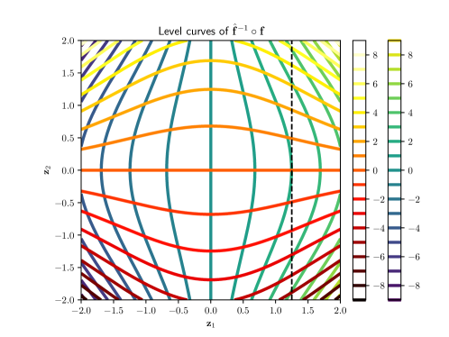
Figure 3: Level curves of the function $\hat{\mathbf{f}}^{-1}\circ\mathbf{f}$ of Example B.1. The cold color scheme corresponds to the level curves of $(\hat{\mathbf{f}}^{-1}\circ\mathbf{f})_{1}(\mathbf{z})$ while the warm color scheme corresponds to $(\hat{\mathbf{f}}^{-1}\circ\mathbf{f})_{2}(\mathbf{z})$. The example gives a concrete case where all assumptions of Theorem 3.1 hold except for the linearity of $\mathbf{f}$. We can see that $\hat{\mathbf{f}}^{-1}\circ\mathbf{f}$ is not a permutation composed with an element-wise invertible transformation, since along the vertical dashed line, we can see that both components of $\hat{\mathbf{f}}^{-1}\circ\mathbf{f}$ change.

Example B.1.

Assume we have 2 latent and 2 observed variables, i.e. $n=2$ and $d=2$. Furthermore, assume that the domain of the causal variables $\mathcal{C}=\mathbb{R}^{2}$ and that Ass. 3.2 and 3.3 hold. For example, consider $\mathbf{C}\sim\mathcal{N}(0,\mathbf{I}_{2})$ with an independent mask $\mathbf{Y}$ with distribution $p(\mathbf{Y}=\mathbf{y})=1/4$ for any $\mathbf{y}\in\{0,1\}^{2}$, which trivially satisfies Ass. 3.2 and 3.3. In this case, the support of $\mathbf{Z}=\mathbf{Y}\odot\mathbf{C}$ is $\mathcal{Z}=\mathbb{R}^{2}$. Assume further that $\mathbf{f}:\mathbb{R}^{2}\rightarrow\mathbb{R}^{2}$ is defined by

$$\mathbf{f}(\mathbf{z}):=\sinh(\mathbf{R}_{\frac{\pi}{4}}\mathbf{z})+\sinh(\mathbf{R}_{-\frac{\pi}{4}}\mathbf{z})\,,$$ (79)

where $\sinh(x):=\frac{e^{x}-e^{-x}}{2}$ (applied element-wise above) and $\mathbf{R}_{\theta}$ is a rotation matrix defined by

$$\mathbf{R}_{\theta}:=\begin{bmatrix}\cos\theta&-\sin\theta\\ \sin\theta&\cos\theta\end{bmatrix}\,.$$ (80)

Consider $\hat{\mathbf{f}}$ and $\mathbf{g}$ to be the identity function. We now show that all the assumptions of Theorem 3.1 except the linearity of $\mathbf{f}$ are satisfied. First, notice how

$$\mathbb{E}||\mathbf{X}-\hat{\mathbf{f}}(\mathbf{g}(\mathbf{X}))||^{2}=\mathbb{E}||\mathbf{X}-\mathbf{X}||^{2}=0\,.$$ (81)

Since $\mathbf{X}=\mathbf{f}(\mathbf{Z})$ by definition and $\mathbf{g}(\mathbf{X})=\mathbf{X}$, since $\mathbf{g}$ is the identity function, then $\mathbf{f}(\mathbf{Z})=\mathbf{g}(\mathbf{X})$ and thus $\mathbb{E}||\mathbf{g}(\mathbf{X})||_{0}=\mathbb{E}||\mathbf{f}(\mathbf{Z})||_{0}$.

We now show that $\mathbb{E}||\mathbf{f}(\mathbf{Z})||_{0}\leq\mathbb{E}||\mathbf{Z}||_{0}$, which we will then use to prove the sparsity condition on $\mathbb{E}||\mathbf{g}(\mathbf{X})||_{0}$.

We can see that

$$\mathbf{f}(\begin{bmatrix}z_{1}\\ 0\end{bmatrix}) =\sinh(z_{1}\begin{bmatrix}\cos\frac{\pi}{4}\\ \sin\frac{\pi}{4}\end{bmatrix})+\sinh(z_{1}\begin{bmatrix}\cos-\frac{\pi}{4}\\ \sin-\frac{\pi}{4}\end{bmatrix})$$ (82)

$$=\sinh(z_{1}\begin{bmatrix}\cos\frac{\pi}{4}\\ \sin\frac{\pi}{4}\end{bmatrix})+\sinh(z_{1}\begin{bmatrix}\cos\frac{\pi}{4}\\ -\sin\frac{\pi}{4}\end{bmatrix})$$ (83)

$$=\begin{bmatrix}2\sinh(z_{1}\cos\frac{\pi}{4})\\ \sinh(z_{1}\sin\frac{\pi}{4})+\sinh(-z_{1}\sin\frac{\pi}{4})\end{bmatrix}$$ (84)

$$=\begin{bmatrix}2\sinh(z_{1}\cos\frac{\pi}{4})\\ \sinh(z_{1}\sin\frac{\pi}{4})-\sinh(z_{1}\sin\frac{\pi}{4})\end{bmatrix}=\begin{bmatrix}2\sinh(z_{1}\cos\frac{\pi}{4})\\ 0\end{bmatrix}\,,$$ (85)

where we use the fact that $\sin$ and $\sinh$ are odd, while $\cos$ is even. An analogous argument shows that

$$\mathbf{f}(\begin{bmatrix}0\\ z_{2}\end{bmatrix}) =\begin{bmatrix}0\\ 2\sinh(z_{2}\cos\frac{\pi}{4})\end{bmatrix}\,.$$ (86)

We can also easily show that $\mathbf{f}(0)=0$. The above shows that, for all $\mathbf{z}\in\mathbb{R}^{2}$, $||\mathbf{f}(\mathbf{z})||_{0}\leq||\mathbf{z}||_{0}$. By taking the expectation on both sides we get the desired result: $\mathbb{E}||\mathbf{f}(\mathbf{Z})||_{0}\leq\mathbb{E}||\mathbf{Z}||_{0}$ and thus $\mathbb{E}||\mathbf{g}(\mathbf{X})||_{0}\leq\mathbb{E}||\mathbf{Z}||_{0}$.

However, we can see in in Figure 3 and in the computation below, $\hat{\mathbf{f}}^{-1}\circ\mathbf{f}=\mathbf{f}$ is not a permutation composed with an element-wise invertible transformation on $\mathbb{R}^{2}$.

$$\mathbf{f}(\begin{bmatrix}z_{1}\\ z_{2}\end{bmatrix}) =\begin{bmatrix}\sinh(\cos\frac{\pi}{4}z_{1}-\sin\frac{\pi}{4}z_{2})+\sinh(\cos\frac{\pi}{4}z_{1}+\sin\frac{\pi}{4}z_{2})\\ \sinh(\sin\frac{\pi}{4}z_{1}+\cos\frac{\pi}{4}z_{2})-\sinh(\sin\frac{\pi}{4}z_{1}-\cos\frac{\pi}{4}z_{2})\end{bmatrix}$$ (87)

This counter-example shows that the results of Theorem 3.1 do not apply in general if $\mathbf{f}$ is nonlinear, but only with additional assumptions, as shown in Theorem 3.4.

Appendix C Extended Related Work

Most closely related to our work are recent identifiability studies, which also explicitly learn causal representations in a partially observable setting. Yao et al. [2023] consider learning from tuples of simultaneously observed views, which depend on different fixed (potentially overlapping) subsets of latents with modality-specific mixing functions, and prove identifiability results for different blocks of shared content variables [von Kügelgen et al., 2021]. Compared to our setting, such paired multi-view data may be harder to obtain. Sturma et al. [2023] study an unpaired, multi-domain setup, in which observations from each domain depend on a different fixed subset of latents, and show identifiability of the causal representation and graph in the fully linear case. This setting resembles our results for the piecewise linear case in Thm. 3.4, where we assume we have the group information for each observation, which can be seen as a single domain. On the other hand, for the linear case in Thm. 3.1, we do not need the group information, hence we also allow for mixtures of data from multiple domains.

Other works in an i.i.d. setting can be viewed as modelling partial observability implicitly by restricting the graph connecting latent and observed variables and establishing identifiability for linear [Adams et al., 2021, Cai et al., 2019, Silva et al., 2006, Xie et al., 2020, 2022] or discrete [Kivva et al., 2021] settings. In our work, we consider the case in which either the causal model or the mixing are not linear and do not constrain the connectivity between $\mathbf{Z}$ and $\mathbf{X}$.

Not considering partial observability, other works on CRL aim to also learn the causal graph from different types (hard/soft, single/multi-node) of interventions in linear [Squires et al., 2023, Bing et al., 2023], partially [Buchholz et al., 2023, Ahuja et al., 2023a, b, Zhang et al., 2023], or fully nonlinear [von Kügelgen et al., 2023, Varici et al., 2023] settings. We focus instead on only recovering the latent causal variables without access to interventional data.

Other works have also explored the piecewise linear setting for identifiability, including with the assumption of Gaussian causal variables. In particular, Thm. 3.4 resembles one of the identifiability results from Kivva et al. [2022] which assumes $\mathbf{Z}$ is a mixture of non-degenerate Gaussians and $\mathbf{f}$ is a piecewise linear function. We note that, in Thm. 3.4, $\mathbf{Z}$ is also a mixture of Gaussians, where the “cluster index” corresponds to $\mathbf{Y}$. However, this mixture contains components which are degenerate, in the sense that their covariances might be singular (this occur when $\mathbf{Y}_{i}=0$ for some $i$). This prevents us from applying the result of Kivva et al. [2022] directly to our setting. On the other hand, although we allow for degenerate components, our result assumes knowledge of the groups $g$, unlike Kivva et al. [2022].

Prior work has also leveraged sparsity in representation learning, for example via a Spike and Slab prior [Tonolini et al., 2020, Moran et al., 2022], or by relating the learnt representation to multiple tasks, each depending only on a small subset of latents [Lachapelle et al., 2023, Fumero et al., 2023]. Most closely related to ours is work by Lachapelle et al. [2022, 2024], who have proposed a sparsity principle for identifiable CRL in interventional and temporal settings, motivated by the sparse mechanism shift hypothesis [Schölkopf et al., 2021, Perry et al., 2022].

Our work is also related to sparse component analysis [Gribonval and Lesage, 2006] and sparse dictionary learning [Mairal et al., 2009]. These unsupervised representation learning methods assume linear mixing functions $\mathbf{f}$ and learn a sparse representations of the input $\mathbf{X}$, similar to our $\mathbf{g}(\mathbf{X})$. The identifiability of dictionary learning has been studied, e.g. by Hu and Huang [2023], in the finite sample regime. The main distinction with our work is that we focus on identifiability with nonlinear mixing.

Appendix D Implementation details

This section provides further details about the experiment implementation in Section 4. The implementation is built upon the code open-sourced by Lachapelle et al. [2022]; Ahuja et al. [2022]; von Kügelgen et al. [2021]; Zheng et al. [2018].

D.1 Hyperparameters

	Numerical linear $\mathbf{f}$	Numerical p.w. linear $\mathbf{f}$	Multiple balls	PartialCausal3DIdent
	Section 5.1	Section 5.1	Section 5.2	Section 5.3
$\epsilon$	0.001	0.01	0.01	0.01
Optimizer	ExtraAdam	ExtraAdam	ExtraAdam	ExtraAdam
Primal optimizer learning rate	1e-4	5e-5	1e-5	1e-4
Dual optimizer learning rate	1e-4/2	5e-5/2	1e-5/2	1e-4/2
Batch size	6144	5000	50$\times K$	13$\times K$
Group number $K$	$2^{n}$	latent size $n$	latent size $n$	10
# Seeds	3	3	3	3
# Iterations	50000	10000	10000	10000

Table 4: Parameters for experiments results in Sec. 5 and App. E.

D.2 Sensitivity analysis on $\epsilon$

We conduct a sensitivity analysis on $\epsilon$. As shown in fig. 4, we observe that the linear case exhibits heightened sensitivity $\epsilon$, whereas the piecewise linear case does not display such sensitivity. We attribute this difference to the additional group and mask information given in the training phase for piecewise linear case, enhancing the method’s robustness to variations in this hyperparameter.

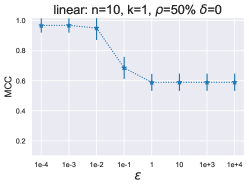
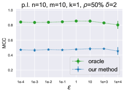
Figure 4: Sensitivity analysis on $\epsilon$ varies from $1e-4$ to $1e4$. The left graph is for the linear case, and right-hand side is for the piecewise linear case.

D.3 Oracle method

In Sec. 4, to encourage Gaussianity of learned representations, we add a regularization term to force the sample skewness and kurtosis to match the Gaussian distribution. However, as we mention in Sec. 4, estimated skewness and kurtosis cannot guarantee Gaussianity. In fig. 5, we empirically show even by adding the two penalty terms into the loss function, the estimator we obtain is still highly non-gaussian.

In the Oracle method, we adopt the assumption of knowing masks in train phases. Instead of directly estimating the unmeasured part as a constant value, we provide less information by replacing $\mathbf{g}_{\psi}(\mathbf{x}_{i})$ with a low standard deviation $e^{-10}$ in Eq. 4; for the measured latent variables, we assign $e$ to $\mathbf{g}_{\psi}(\mathbf{x}_{i})$. After training, we obtain the encoder function $\mathbf{g}$. In the test phase, data in distinct groups can be mixed together. There is no longer a requirement for mask-related information. In addition, we find empirically that if we replace $\hat{\bm{\mu}}_{g}$ with a constant value, e.g. 5, it also enhances the performance.

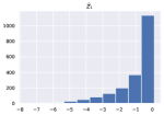
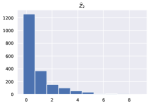
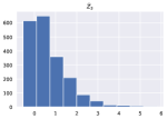
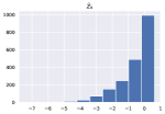
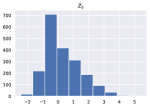
Figure 5: Histogram of estimator for our method for $n=5$, $m=10$, independent $\mathbf{Z}$, $\rho$=50%,

D.4 Predefined masks

In order to satisfy Ass. 2.2, i.e. for each latent variable $C_{i}$ $i\in[n]$, all the other latent variables should be measured in at least one of the groups where $C_{i}$ is unmeasured, the minimum number of distinct masks is equal to the latent size $n$, and the maximum number is up to $2^{n}$. In this paper, we consider 3 different strategies to generate masks.

• Consider all $2^{n}$ possible masks as a mask set $\mathbf{Y}$. For each data $\mathbf{c}^{i}$, $i\in[N]$, we uniformly sample one mask $\mathbf{y}^{i}$ from the mask set $\mathbf{Y}$. This strategy is used in numerical experiments with linear $\mathbf{f}$ since we do not need group-wise masks.

• Define $n$ possible masks $\{\mathbf{y}_{1},..,\mathbf{y}_{n}\}$ with the same ratio of measured variables $\rho$. Define $\mathbf{y}_{g}$, $g=[n]$ by this way: set $g$-th to $(g+\rho n)$-th element as 1, the rest are 0s. This strategy is used in numerical experiments with piecewise linear $\mathbf{f}$ and multiple balls experiment due to the necessity of having a specific number of samples from the same group in each batch for the computation of sample skewness and kurtosis—something strategy i) is incapable of achieving.

• Define $n$ possible masks $\{\mathbf{y}_{1},..,\mathbf{y}_{n}\}$ with different ratio of measured variables $\rho_{g}$, $g=[n]$ from 1 var to 100%. Define $\mathbf{y}_{g}$ this way: set $1$-th to $(g+\rho_{g}n)$-th element as 1, the rest are 0s. This is employed in the PartialCausal3DIdent experiment.

Appendix E Full experimental results

E.1 Numerical experiments

E.1.1 Linear mixing function

We first show the Pearson Correlation matrix $\mathrm{Corr}^{n\times n}_{\pi}$ with the permutation $\pi$ between ground truth latent variables $\mathbf{Z}$ and the estimator $\hat{\mathbf{Z}}=\mathbf{g}(\mathbf{X})$. One figure represents one ablation study in table 1. We choose one random seed to plot for each setup. Ground truth Pear. Corr. matrix on the left shows the original linear correlation inside $\mathbf{Z}$, compared with the estimator on the right-hand side.

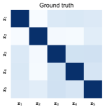
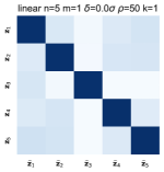
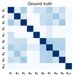
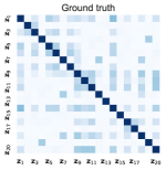
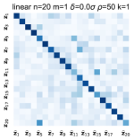
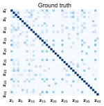
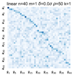
Figure 6: ER+Linear Gaussian noise: ablation study on latent dimension $n$

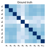
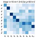
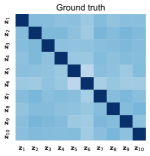
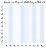
Figure 7: ER+Linear Gaussian noise: ablation study on graph dense ER-k

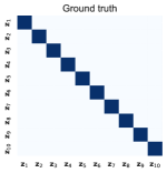
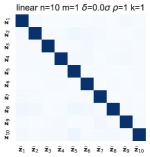
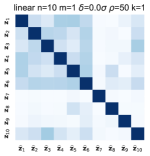
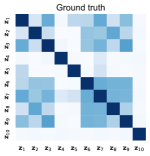
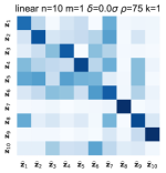
Figure 8: ER+Linear Gaussian noise: ablation study on ratio of measured latent variables $\rho$

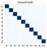
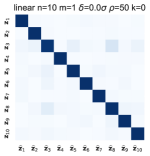
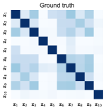
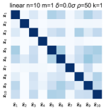
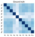
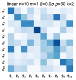
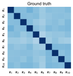
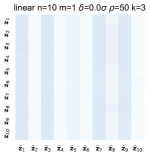
Figure 9: ER+Linear Exponential noise: ablation study on graph dense ER-k

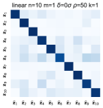
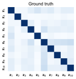
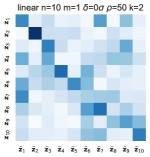
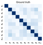
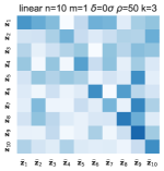
Figure 10: ER+nonlinear: ablation study on graph dense ER-k

To exclude the natural dependency between latent variables that potentially enhance the value of metric MCC, we provide additional experiment results with independent latent variables in table 5.

Table 5: Results for the numerical experiments in the linear case when $\mathbf{Z}$ are independent.

$n$	Causal Graph	$\rho$	MCC
5	Independent	50 %	0.998$\pm$0.000
10	Independent	50 %	0.988$\pm$0.014
20	Independent	50 %	0.957$\pm$0.027
40	Independent	50 %	0.702$\pm$0.047
10	Independent	1var	0.998 $\pm$0.001
10	Independent	50 %	0.988$\pm$0.014
10	Independent	75 %	0.876 $\pm$0.095

E.1.2 Piecewise linear mixing function

In table 6 and table 7, we provide the numerical results of averaged MCC and standard deviation over 3 random seeds as shown in fig. 2. In the second block of table 6, we provide two additional results of our method (training without mask information) when $\mathbf{Z}$ are independent. In table 7, the second right column is for training without mask information, and the most right column is the oracle method, i.e., providing mask information in the training phase. Additionally, to exclude the natural dependency between latent variables that potentially enhance the value of metric MCC, we provide additional experiment results with independent latent variables in table 8.

Table 6: Results for the numerical experiments in the piecewise linear case for simple settings.

$n$	$m$	$k$	$\rho$	$\delta$	MCC (mean $\pm$ std)
3	3	1	50 %	0	0.656$\pm$0.105
3	3	1	50 %	2	0.716$\pm$0.025
3	3	1	50 %	3	0.860$\pm$0.084
3	3	1	50 %	5	0.864$\pm$0.042
3	3	1	50 %	10	0.875$\pm$0.032
3	3	0	50 %	2	0.817$\pm$0.030
3	3	0	50 %	3	0.874$\pm$0.028

Table 7: Results for the numerical experiments in the piecewise linear case for the dependent variable case.

$n$	$m$	$k$	$\rho$	$\delta$	MCC (mean $\pm$ std)	MCC (mean $\pm$ std) oracle
5	10	1	50 %	2	0.622$\pm$0.139	0.916$\pm$0.009
10	10	1	50 %	2	0.477$\pm$0.004	0.846$\pm$0.004
20	10	1	50 %	2	0.475$\pm$0.031	0.816$\pm$0.011
40	10	1	50 %	2	0.435$\pm$0.028	0.803$\pm$0.001
10	10	1	50 %	2	0.477$\pm$0.005	0.846$\pm$0.004
10	10	2	50 %	2	0.505$\pm$0.024	0.877$\pm$0.014
10	10	3	50 %	2	0.502$\pm$0.021	0.880$\pm$0.004
10	10	1	50 %	2	0.642$\pm$0.017	0.857$\pm$0.002
10	10	1	50 %	2	0.477$\pm$0.005	0.846$\pm$0.004
10	20	1	50 %	2	0.412$\pm$0.041	0.716$\pm$0.039
10	10	1	1var	2	0.433$\pm$0.054	0.930$\pm$0.010
10	10	1	50 %	2	0.477$\pm$0.005	0.846$\pm$0.004
10	10	1	75 %	2	0.411$\pm$0.12	0.757$\pm$0.008
10	10	1	50 %	0	0.344$\pm$0.023	0.360$\pm$0.024
10	10	1	50 %	3	0.498$\pm$0.029	0.907$\pm$0.003
10	10	1	50 %	5	0.552$\pm$0.024	0.961$\pm$0.002
10	10	1	50 %	10	0.543$\pm$0.030	0.990$\pm$0.000

Table 8: Results for the numerical experiments in the piecewise linear case for the independent variable case.

$n$	$m$	$k$	$\rho$	$\delta$	MCC (mean $\pm$ std)	MCC (mean $\pm$ std) oracle
5	10	0	50 %	2	0.571$\pm$0.134	0.910$\pm$0.004
10	10	0	50 %	2	0.476$\pm$0.043	0.837$\pm$0.008
20	10	0	50 %	2	0.467$\pm$0.008	0.801$\pm$0.005
40	10	0	50 %	2	0.415$\pm$0.031	0.792$\pm$0.003
10	3	0	50 %	2	0.618$\pm$0.019	0.853$\pm$0.003
10	10	0	50 %	2	0.476$\pm$0.043	0.837$\pm$0.008
10	20	0	50 %	2	0.430$\pm$0.036	0.689$\pm$0.035
10	10	0	1var	2	0.545$\pm$0.103	0.925$\pm$0.014
10	10	0	50 %	2	0.476$\pm$0.043	0.837$\pm$0.008
10	10	0	75 %	2	0.596$\pm$0.103	0.695$\pm$0.041
10	10	0	50 %	0	0.344$\pm$0.023	0.309$\pm$0.059
10	10	0	50 %	3	0.529$\pm$0.038	0.907$\pm$0.003
10	10	0	50 %	5	0.582$\pm$0.045	0.961$\pm$0.003

For each setup in table 7, we choose one random seed to plot the heatmap of the Pearson Correlation matrix $\mathrm{Corr}^{n\times n}_{\pi}$ with the permutation $\pi$ . One figure represents one ablation study of one parameter. Ground truth Pear. Corr. matrix on the left shows the original linear correlation inside Z, compared with the estimator on the right-hand side.

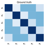
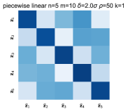
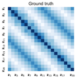
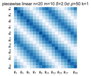
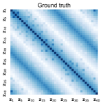
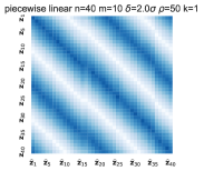
Figure 11: Ablation study on latent dimension $n$

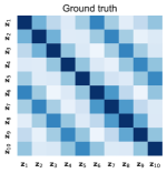
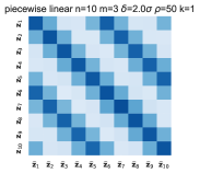
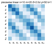
Figure 12: Ablation study on number of layers $m$

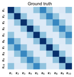
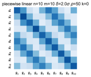
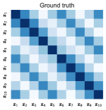
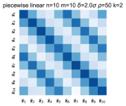
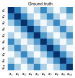
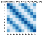
Figure 13: Ablation study on graph density ER-k

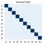
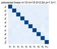
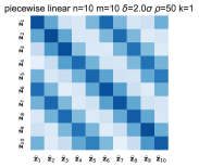
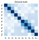
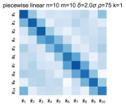
Figure 14: Ablation study on ratio of measured latent variables $\rho$

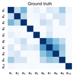
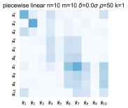
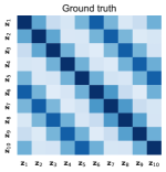
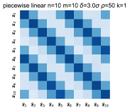
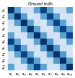
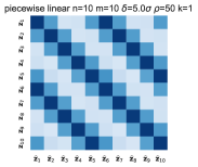
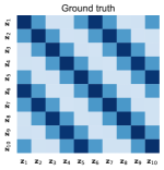
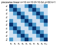
Figure 15: Ablation study on mask value $\delta$

E.2 Image dataset: Multiple Balls

Data generation process

We use PyGame [Shinners, 2011] to render images with size $64\times 64\times 3$ as shown in fig. 16. The number of balls $b$ varies from 2 to 8.

For the missing ball setting, we generate the $x$-coordinates of each ball $\mathbf{C}_{j}$ for $j\in[b]$ from a truncated normal distribution $\mathcal{N}(0.5,0.1^{2})$ with bounds $(0.1,0.9)$. For the masked position setting, we generate the $x$ and $y$-coordinates of each ball $\mathbf{C}_{i}$ for $j\in[b]$ independently from a truncated 2-dimensional normal distribution $\mathcal{N}(\bm{\mu}_{j},\bm{\Sigma}_{j})$ with bounds $(0.1,0.9)^{2}$, where $\bm{\mu}_{i}$ is generated from Unif$(0.4,0.6)^{2}$, and $\bm{\Sigma}_{j}=((0.01,0.005)(0.005,0.01))$ for all groups. All the aforementioned parameters, including mean and variance/covariance above, are configured to ensure the majority of the samples are located in interval $[0,1]$. This configuration aims to maintain the truncated distribution as close to a Gaussian distribution as feasible.

For both settings, we generate the masked causal variables as $(\mathbf{Z}_{k})^{K}_{k=1}=\mathbf{y}\cdot\mathbf{C}+(1-\mathbf{y})\cdot\mathbf{M}\in\mathbb{R}^{K\times n}$. For the missing ball setting, the latent size is equal to the number of balls $\mathbf{b}$. Therefore, we predefine $b$ masks via strategy ii) in App. D.4. The mask value is set as $\mathbf{0}$. For the masked position setting, the latent size is $2b$ since both $x$ and $y$-coordinates of each ball are considered. The masked positions for distinct balls are different; avoiding overlap happens if two balls are masked in the same group. The mask value of each latent is predefined by one of these values {0.05, 0.1, 0.9, 0.95}.

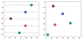
Figure 16: Example images of two settings in multiple ball dataset, based on the rendering code provided by [Ahuja et al., 2022]. (left) Missing ball setting: balls can move along gray paths only and are not visible when they move out of view. (right) Masked position setting: balls can move freely inside the frame and their coordinates are masked when they have a specific value $\mathbf{M}$; e.g., the left-bottom position represents a masked version of the $x$ and $y$ coordinate for the olive ball.

E.3 Image dataset: Causal3DIdent

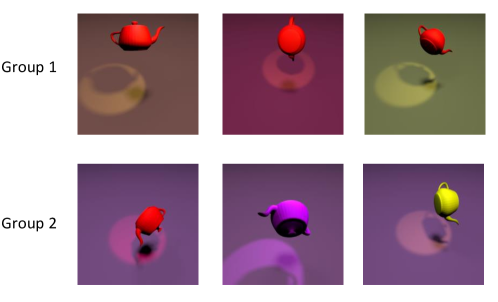
Figure 17: Example images from two groups in PartialCausal3DIdent dataset, resampled from Causal3DIdent datasert provided by [von Kügelgen et al., 2021]. In Group 1, the variable object hue is masked to a constant. In Group 2, the variable background hue is masked to a constant.

A qualitative visualization of the result for one object class is presented in Fig. 18 where estimated and ground truth latent are well aligned on the diagonal.

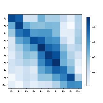
Figure 18: Pearson correlation matrix $\mathrm{Corr}^{n\times n}_{\pi}$ with the permutation $\pi$ between estimated and ground truth latent variables for PartialCausal3DIdent with masking distance $\delta=10\sigma$ for all latent variables.

Since as we show in table 3, we did not observe significant performance differences between different object classes, we conduct an ablation study of the masking value $\delta$ only on Object Class ID 0. We show the results in table 9. Consistent with the observation in numerical experiments, when we increase the value of $\delta$, which measures the distance between mask value and original mean, our method achieves better identification.

Table 9: MCC on object class ID=0 regarding various masking values $\delta$ with standard deviation $\sigma=0.1$. Results averaged over three random seeds.

$\mathrm{\delta}$	0	$2\sigma$	$3\sigma$	$5\sigma$
MCC (mean $\pm$ std)	$0.586\pm 0.056$	$0.632\pm 0.044$	$0.700\pm 0.039$	$0.828\pm 0.011$

Appendix F Image credits

The images in Fig. 1 are adapted from a VectorPortal image that is covered by CC BY 4.0. We segmented the cars, and removed some of them or moved their position in the image.

References

- Adams et al. (2021) Jeffrey Adams, Niels Hansen, and Kun Zhang. Identification of partially observed linear causal models: Graphical conditions for the non-gaussian and heterogeneous cases. Advances in Neural Information Processing Systems, 34:22822–22833, 2021.
- Ahuja et al. (2022) Kartik Ahuja, Jason S Hartford, and Yoshua Bengio. Weakly supervised representation learning with sparse perturbations. Advances in Neural Information Processing Systems, 35:15516–15528, 2022.
- Ahuja et al. (2023a) Kartik Ahuja, Divyat Mahajan, Yixin Wang, and Yoshua Bengio. Interventional causal representation learning. In International Conference on Machine Learning, pages 372–407. PMLR, 2023a.
- Ahuja et al. (2023b) Kartik Ahuja, Amin Mansouri, and Yixin Wang. Multi-domain causal representation learning via weak distributional invariances. In Causal Representation Learning Workshop at NeurIPS 2023, 2023b.
- Bing et al. (2023) Simon Bing, Urmi Ninad, Jonas Wahl, and Jakob Runge. Identifying linearly-mixed causal representations from multi-node interventions. arXiv preprint arXiv:2311.02695, 2023.
- Brehmer et al. (2022) Johann Brehmer, Pim De Haan, Phillip Lippe, and Taco S Cohen. Weakly supervised causal representation learning. Advances in Neural Information Processing Systems, 35:38319–38331, 2022.
- Buchholz et al. (2023) Simon Buchholz, Goutham Rajendran, Elan Rosenfeld, Bryon Aragam, Bernhard Schölkopf, and Pradeep Ravikumar. Learning linear causal representations from interventions under general nonlinear mixing. In Advances in Neural Information Processing Systems, 2023.
- Cai et al. (2019) Ruichu Cai, Feng Xie, Clark Glymour, Zhifeng Hao, and Kun Zhang. Triad constraints for learning causal structure of latent variables. Advances in neural information processing systems, 32, 2019.
- Comon (1994) P. Comon. Independent component analysis, a new concept? Signal Processing, 1994.
- Friedberg et al. (2014) S.H. Friedberg, A.J. Insel, and L.E. Spence. Linear Algebra. Pearson Education, 2014. ISBN 9780321998897.
- Fumero et al. (2023) Marco Fumero, Florian Wenzel, Luca Zancato, Alessandro Achille, Emanuele Rodolà, Stefano Soatto, Bernhard Schölkopf, and Francesco Locatello. Leveraging sparse and shared feature activations for disentangled representation learning. arXiv preprint arXiv:2304.07939, 2023.
- Gallego-Posada and Ramirez (2022) Jose Gallego-Posada and Juan Ramirez. Cooper: a toolkit for lagrangian-based constrained optimization, 2022.
- Gidel et al. (2018) Gauthier Gidel, Hugo Berard, Gaëtan Vignoud, Pascal Vincent, and Simon Lacoste-Julien. A variational inequality perspective on generative adversarial networks. arXiv preprint arXiv:1802.10551, 2018.
- Gribonval and Lesage (2006) Rémi Gribonval and Sylvain Lesage. A survey of sparse component analysis for blind source separation: principles, perspectives, and new challenges. In ESANN’06 proceedings-14th European Symposium on Artificial Neural Networks, pages 323–330. d-side publi., 2006.
- Hu and Huang (2023) Jingzhou Hu and Kejun Huang. Global identifiability of $\ell_1$-based dictionary learning via matrix volume optimization. In Thirty-seventh Conference on Neural Information Processing Systems, 2023.
- Hyvarinen and Morioka (2016) Aapo Hyvarinen and Hiroshi Morioka. Unsupervised feature extraction by time-contrastive learning and nonlinear ica. Advances in neural information processing systems, 29, 2016.
- Hyvarinen and Morioka (2017) Aapo Hyvarinen and Hiroshi Morioka. Nonlinear ica of temporally dependent stationary sources. In Artificial Intelligence and Statistics, pages 460–469. PMLR, 2017.
- Hyvarinen et al. (2019) Aapo Hyvarinen, Hiroaki Sasaki, and Richard Turner. Nonlinear ica using auxiliary variables and generalized contrastive learning. In The 22nd International Conference on Artificial Intelligence and Statistics, pages 859–868. PMLR, 2019.
- Khemakhem et al. (2020) Ilyes Khemakhem, Diederik Kingma, Ricardo Monti, and Aapo Hyvarinen. Variational autoencoders and nonlinear ica: A unifying framework. In International Conference on Artificial Intelligence and Statistics, pages 2207–2217. PMLR, 2020.
- Kivva et al. (2021) Bohdan Kivva, Goutham Rajendran, Pradeep Ravikumar, and Bryon Aragam. Learning latent causal graphs via mixture oracles. Advances in Neural Information Processing Systems, 34:18087–18101, 2021.
- Kivva et al. (2022) Bohdan Kivva, Goutham Rajendran, Pradeep Ravikumar, and Bryon Aragam. Identifiability of deep generative models without auxiliary information. Advances in Neural Information Processing Systems, 35:15687–15701, 2022.
- Lachapelle et al. (2022) Sébastien Lachapelle, Pau Rodriguez, Yash Sharma, Katie E Everett, Rémi Le Priol, Alexandre Lacoste, and Simon Lacoste-Julien. Disentanglement via mechanism sparsity regularization: A new principle for nonlinear ica. In Conference on Causal Learning and Reasoning, pages 428–484. PMLR, 2022.
- Lachapelle et al. (2023) Sébastien Lachapelle, Tristan Deleu, Divyat Mahajan, Ioannis Mitliagkas, Yoshua Bengio, Simon Lacoste-Julien, and Quentin Bertrand. Synergies between disentanglement and sparsity: Generalization and identifiability in multi-task learning. In International Conference on Machine Learning, pages 18171–18206. PMLR, 2023.
- Lachapelle et al. (2024) Sébastien Lachapelle, Pau Rodríguez López, Yash Sharma, Katie Everett, Rémi Le Priol, Alexandre Lacoste, and Simon Lacoste-Julien. Nonparametric partial disentanglement via mechanism sparsity: Sparse actions, interventions and sparse temporal dependencies, 2024.
- Lippe et al. (2022) Phillip Lippe, Sara Magliacane, Sindy Löwe, Yuki M Asano, Taco Cohen, and Stratis Gavves. Citris: Causal identifiability from temporal intervened sequences. In International Conference on Machine Learning, pages 13557–13603. PMLR, 2022.
- Lippe et al. (2023) Phillip Lippe, Sara Magliacane, Sindy Löwe, Yuki M Asano, Taco Cohen, and Efstratios Gavves. Biscuit: Causal representation learning from binary interactions. Proceedings of the Thirty-Ninth Conference on Uncertainty in Artificial Intelligence, 2023.
- Mairal et al. (2009) J. Mairal, F. Bach, J. Ponce, and G. Sapiro. Online dictionary learning for sparse coding. In Proceedings of the 26th annual international conference on machine learning, pages 689–696, 2009.
- Moran et al. (2022) G Moran, D Sridhar, Y Wang, and D Blei. Identifiable deep generative models via sparse decoding. Transactions on machine learning research, 2022.
- Pearl (2009) Judea Pearl. Causality: Models, Reasoning and Inference. Cambridge University Press, USA, 2nd edition, 2009. ISBN 052189560X.
- Perry et al. (2022) Ronan Perry, Julius Von Kügelgen, and Bernhard Schölkopf. Causal discovery in heterogeneous environments under the sparse mechanism shift hypothesis. Advances in Neural Information Processing Systems, 35:10904–10917, 2022.
- Peters et al. (2017) Jonas Peters, Dominik Janzing, and Bernhard Schlkopf. Elements of Causal Inference: Foundations and Learning Algorithms. The MIT Press, 2017. ISBN 0262037319.
- Schölkopf et al. (2021) Bernhard Schölkopf, Francesco Locatello, Stefan Bauer, Nan Rosemary Ke, Nal Kalchbrenner, Anirudh Goyal, and Yoshua Bengio. Toward causal representation learning. Proceedings of the IEEE, 109(5):612–634, 2021.
- Shinners (2011) Pete Shinners. Pygame, 2011.
- Silva et al. (2006) Ricardo Silva, Richard Scheines, Clark Glymour, Peter Spirtes, and David Maxwell Chickering. Learning the structure of linear latent variable models. Journal of Machine Learning Research, 7(2), 2006.
- Spirtes et al. (2000) Peter Spirtes, Clark Glymour, and Richard Scheines. Causation, Prediction, and Search. MIT Press, Cambridge MA, 2nd edition, 2000.
- Squires et al. (2023) Chandler Squires, Anna Seigal, Salil Bhate, and Caroline Uhler. Linear causal disentanglement via interventions. In 40th International Conference on Machine Learning, 2023.
- Sturma et al. (2023) Nils Sturma, Chandler Squires, Mathias Drton, and Caroline Uhler. Unpaired multi-domain causal representation learning. Thirty-seventh Conference on Neural Information Processing Systems, 2023.
- Tonolini et al. (2020) Francesco Tonolini, Bjørn Sand Jensen, and Roderick Murray-Smith. Variational sparse coding. In Uncertainty in Artificial Intelligence, pages 690–700. PMLR, 2020.
- Varici et al. (2023) Burak Varici, Emre Acartürk, Karthikeyan Shanmugam, and Ali Tajer. Score-based causal representation learning from interventions: Nonparametric identifiability. In Causal Representation Learning Workshop at NeurIPS 2023, 2023.
- von Kügelgen et al. (2021) Julius von Kügelgen, Yash Sharma, Luigi Gresele, Wieland Brendel, Bernhard Schölkopf, Michel Besserve, and Francesco Locatello. Self-supervised learning with data augmentations provably isolates content from style. Advances in neural information processing systems, 34:16451–16467, 2021.
- von Kügelgen et al. (2023) Julius von Kügelgen, Michel Besserve, Wendong Liang, Luigi Gresele, Armin Kekić, Elias Bareinboim, David M Blei, and Bernhard Schölkopf. Nonparametric identifiability of causal representations from unknown interventions. In Advances in Neural Information Processing 36, 2023.
- Wendong et al. (2023) Liang Wendong, Armin Kekić, Julius von Kügelgen, Simon Buchholz, Michel Besserve, Luigi Gresele, and Bernhard Schölkopf. Causal component analysis. In Advances in Neural Information Processing Systems, 2023.
- Xie et al. (2020) Feng Xie, Ruichu Cai, Biwei Huang, Clark Glymour, Zhifeng Hao, and Kun Zhang. Generalized independent noise condition for estimating latent variable causal graphs. Advances in neural information processing systems, 33:14891–14902, 2020.
- Xie et al. (2022) Feng Xie, Biwei Huang, Zhengming Chen, Yangbo He, Zhi Geng, and Kun Zhang. Identification of linear non-gaussian latent hierarchical structure. In International Conference on Machine Learning, pages 24370–24387. PMLR, 2022.
- Yao et al. (2023) Dingling Yao, Danru Xu, Sébastien Lachapelle, Sara Magliacane, Perouz Taslakian, Georg Martius, Julius von Kügelgen, and Francesco Locatello. Multi-view causal representation learning with partial observability. arXiv preprint arXiv:2311.04056, 2023.
- Yao et al. (2022) Weiran Yao, Yuewen Sun, Alex Ho, Changyin Sun, and Kun Zhang. Learning temporally causal latent processes from general temporal data. In International Conference on Learning Representations, 2022.
- Zhang et al. (2023) Jiaqi Zhang, Kristjan Greenewald, Chandler Squires, Akash Srivastava, Karthikeyan Shanmugam, and Caroline Uhler. Identifiability guarantees for causal disentanglement from soft interventions. In Advances in Neural Information Processing Systems, 2023.
- Zheng et al. (2018) Xun Zheng, Bryon Aragam, Pradeep K Ravikumar, and Eric P Xing. Dags with no tears: Continuous optimization for structure learning. Advances in neural information processing systems, 31, 2018.