DrivAerNet: A Parametric Car Dataset for Data-Driven Aerodynamic Design and Graph-Based Drag Prediction

Аннотация

This study introduces DrivAerNet, a large-scale high-fidelity CFD dataset of 3D industry-standard car shapes, and RegDGCNN, a dynamic graph convolutional neural network model, both aimed at aerodynamic car design through machine learning. DrivAerNet, with its 4000 detailed 3D car meshes using 0.5 million surface mesh faces and comprehensive aerodynamic performance data comprising of full 3D pressure, velocity fields, and wall-shear stresses, addresses the critical need for extensive datasets to train deep learning models in engineering applications. It is 60% larger than the previously available largest public dataset of cars, and is the only open-source dataset that also models wheels and underbody. RegDGCNN leverages this large-scale dataset to provide high-precision drag estimates directly from 3D meshes, bypassing traditional limitations such as the need for 2D image rendering or Signed Distance Fields (SDF). By enabling fast drag estimation in seconds, RegDGCNN facilitates rapid aerodynamic assessments, offering a substantial leap towards integrating data-driven methods in automotive design. Together, DrivAerNet and RegDGCNN promise to accelerate the car design process and contribute to the development of more efficient vehicles. To lay the groundwork for future innovations in the field, the dataset and code used in our study are publicly accessible at https://github.com/Mohamedelrefaie/DrivAerNet.

Dataset	Size	Aerodynamics Data				Wheels/Underbody	Parametric	Design Parameters	Open-source
		$C_{d}$	$C_{l}$	u	$p$	Modeling
Baque el al. 2018 [7]	2,000	✔	✗	✗	✗	✗	✔	21 (3D)	✗
Umetani et. al 2018 [40]	889	✔	✗	✔	✔	✗	✗	-	✔
Gunpinar et. al 2019 [16]	1,000	✔	✗	✗	✗	✗	✔	21 (2D)	✗
Remelli et. al 2020 [28]	1,400	✗	✗	✗	✔	✗	✗	-	✗
Jacob et. al 2021 [19]	1,000	✔	✔	✔	✗	✔	✔	15 (3D)	✗
Usama et. al 2021 [41]	500	✔	✗	✗	✗	✗	✔	40 (2D)	✗
Rios et. al 2021 [31]	600	✔	✔	✗	✗	✗	✗	-	✗
Song et. al 2023 [36]	2,474	✔	✗	✗	✗	✗	✗	-	✔
Li et. al 2023 [22]	551	✔	✗	✗	✔	✗	✔	6 (3D)	✗
	611	✔	✗	✗	✔	✗	✗	-	✗
Trinh et. al 2024 [39]	1,121	✗	✗	✔	✔	✗	✗	-	✗
DrivAerNet (Ours)	4,000	✔	✔	✔	✔	✔	✔	50 (3D)	✔

Таблица 1: A comparative analysis of various aerodynamics datasets, highlighting key aspects such as number of designs in the dataset (size), the inclusion of aerodynamic coefficients (drag coefficient $C_{d}$ and lift coefficient $C_{l}$), the inclusion of velocity (u) and pressure ($p$) fields, the presence of wheels/underbody modeling, the capacity for conducting parametric studies, the number of design parameters, and open-source availability.

1 Introduction

Reducing fuel consumption and CO2 emissions through advanced aerodynamic design is crucial to the automobile industry. This can help with faster transition towards electric cars, complementing the 2035 ban on internal combustion engine cars and aligning with the ambitious goal of achieving carbon neutrality by 2050 to combat global warming [25, 9, 23]. In aerodynamic design, navigating through intricate design choices involves a detailed examination of aerodynamic performance and design constraints, which is often slowed down by the time-consuming nature of high-fidelity CFD simulations and experimental wind tunnel tests. High-fidelity CFD simulations can take days to weeks per design [6], while wind tunnel testing, despite its accuracy, is limited to examining only a handful of designs due to time and cost constraints. Data-driven approaches can alleviate this bottleneck by leveraging existing datasets to navigate through design and performance spaces, thereby speeding up the design exploration process and efficiently assessing aerodynamic designs.

Although recent advancements in data-driven approaches for aerodynamic design are promising, these typically concentrate on simpler 2D cases [14, 38] or lower-fidelity CFD simulations [36, 22, 7] and overlook the complexities inherent in real-world 3D designs and the challenges posed by high-fidelity CFD simulations. According to [17], simplifying car designs by excluding components like wheels and mirrors, and not modeling the underbody, leads to a significant underestimation of aerodynamic drag. Taking these elements into account increased the drag by more than 1.4 times, highlighting the importance of detailed modeling for accurate aerodynamic analysis. Additionally, there is a dearth of publicly available high-fidelity car simulation datasets, potentially slowing down research in data-driven method development, as each researcher may need extensive computational resources to create their own data and test their methods on them.

Responding to this challenge, our paper introduces DrivAerNet, a comprehensive dataset that features full 3D flow field information across 4000 high-fidelity car CFD simulations. It is made publicly available to serve as a benchmark for training deep learning models in aerodynamic assessment, generative design, and other machine learning applications.

To demonstrate the importance of large-scale datasets, we also develop a surrogate model for aerodynamic drag prediction based on Dynamic Graph Convolutional Neural Networks  [42]. Our model, RegDGCNN, operates directly on extremely large 3D meshes, eliminating the necessity for 2D image rendering or Signed Distance Fields (SDF) generation. RegDGCNN’s ability to swiftly identify aerodynamic improvements opens new avenues for creating more efficient vehicles by streamlining the evaluation of design adjustments. It marks a significant step towards optimizing car designs more efficiently.

Overall, the contributions of this paper are:

• The release of DrivAerNet, an extensive high-fidelity dataset featuring 4000 car designs, complete with detailed 3D models with 0.5 million surface mesh faces each, full 3D flow fields, and aerodynamic performance coefficients. The dataset is 60% larger than the previously available largest public dataset of cars, and is the only open-source dataset that also models wheels and underbody, allowing accurate estimation of drag.

• The introduction of a surrogate model, named RegDGCNN, based on Dynamic Graph Convolutional Neural Networks for prediction of aerodynamic drag. RegDGCNN outperforms state-of-the-art attention-based models [3, 36] for drag prediction by 3.57$\%$ on ShapeNet benchmark dataset while using 1000$\times$ fewer parameters, and achieves an $R^{2}$ score of 0.9 on the DrivAerNet dataset.

In addition, the large size of our dataset is also justified by our analysis in Section 5.3, which reveals that expanding the training dataset from 560 to 2800 car designs from DrivAerNet resulted in a 75$\%$ decrease in error, illustrating the direct correlation between dataset size and model performance. A similar trend is observed with the dataset from [36], where enlarging the number of training samples from 1270 to 6352 entries yielded a 56$\%$ error reduction, further validating our model’s efficacy and the inherent value of large datasets in driving advancements in surrogate modeling.

The structure of our paper is as follows: Section 2 provides an overview of related work. Section 3 presents the DrivAerNet dataset, detailing the numerical simulation methods, CFD results, geometric feasibility analysis, and dataset characteristics. In Section 4, we introduce our RegDGCNN approach using the Dynamic Graph Convolutional Neural Network for regression tasks. Section 5 examines the application of the RegDGCNN model for surrogate modeling of aerodynamic drag, comparing its performance on the DrivAerNet and ShapeNet datasets and underscoring the benefits of scaling the training dataset. The paper highlights the limitations of our study and suggests avenues for future research, followed by a conclusion that summarizes the results and key findings.

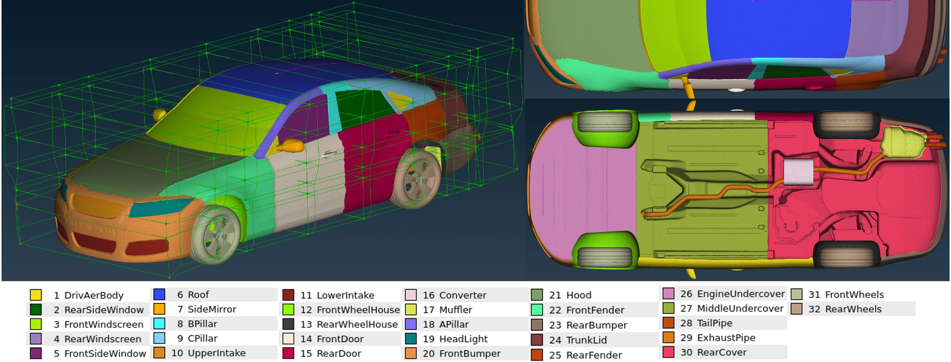
Рис. 1: The parametric DrivAer model is depicted with morphing boxes applied for geometry transformation in ANSA® software using a total of 50 geometric parameters and 32 morphable entities. The morphing boxes are color-coded to highlight the areas susceptible to parametric modifications, facilitating the creation of ‘DrivAerNet’ dataset. Utilizing this morphing technique, we generated 4,000 unique car designs.

2 Related Work

This section starts with an overview of aerodynamics datasets, and then transitions to discussing recent progress in 3D learning for aerodynamics.

2.1 Aerodynamics Datasets

Data-driven aerodynamic design is a methodology that leverages computational models and machine learning algorithms to optimize car shapes based on large volumes of aerodynamic performance data, aiming to improve efficiency and performance. A common type of data-driven aerodynamic design is surrogate modeling, which uses simplified models to approximate the behavior of complex aerodynamic phenomena, enabling faster simulations and iterations in the design process. It is particularly useful for preliminary design phases where quick evaluations are necessary. However, a significant portion of existing research on data-driven aerodynamic design is concentrated on simplified 2D scenarios such as airfoils/2D geometries [8, 38, 14, 41, 20, 16] or simplified 3D models [7, 28, 22, 40, 31, 36, 39]. While these studies are instrumental in understanding the fundamental physics, they often fall short in terms of applicability to complex 3D real-world problems. This gap is further widened by the absence of proprietary data from the industry, posing challenges in replicating and validating research findings. Moreover, the absence of a standardized benchmark dataset in the field hampers the ability to consistently evaluate and compare the efficacy of various machine learning methodologies. This stands in contrast to fields such as image processing or 3D shape analysis, where benchmark datasets like ImageNet [13] or ShapeNet [10] have accelerated significant advancements in deep learning by providing a common ground for methods comparison. Although benchmarks for CFD simulations and turbulence modeling [4, 5, 6] do exist, their limited size often renders them inadequate for the demands of deep learning techniques, underscoring the necessity for a broader and more comprehensive dataset.

Table  1 provides an overview of existing datasets in the literature for data-driven aerodynamic design. It compares their size, the inclusion of aerodynamic information such as drag coefficient ($C_{d}$), lift coefficient ($C_{l}$), velocity field (u), pressure ($p$), whether they are parametric, the number of design parameters, and their availability as open-source. In addition, we consider the modeling of the rotating wheels and underbody for evaluation. Our dataset stands out with the largest size of 4,000 samples, comprehensive aerodynamic information, parametric details, modeling of the wheels and underbody, and open-source accessibility.

Below, we discuss recent advancements in 3D learning for aerodynamics.

(a) Fastback configuration of the DrivAer baseline model with detailed underbody, mirrors, and wheels.

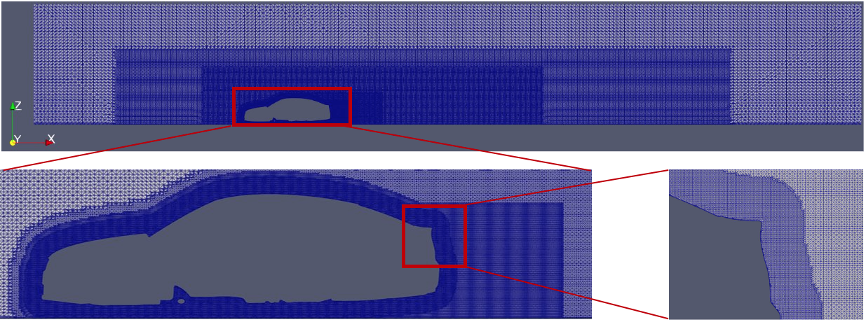
(b) Computational grid in the $y$-normal symmetry plane displays four distinct regions of refinement. The addition of layers around the car body is also evident, all designed to accurately capture both the wake dynamics and the boundary layer development.

Рис. 2: DrivAer Fastback model, complete with detailed features, alongside its computational mesh, illustrating the mesh refinement zones and additional layers aimed at accurately modeling aerodynamic phenomena.

2.2 Advancements in 3D Learning for Aerodynamics

The study from [39] presented a super-resolution model aimed at refining the estimated, yet coarsely resolved, flow fields around vehicles from deep learning predictions to a higher resolution, crucial for aerodynamic vehicle design. By incorporating a residual-in-residual dense block (RRDB) within the generator structure and employing a relativistic discriminator for enhanced detail capture, coupled with a novel distance-weighted loss and physics-informed loss to ensure physical accuracy, the methodology demonstrated a marked improvement in flow field enhancement around vehicles, outperforming previous approaches in this domain. Jacob et. al [19] demonstrated that deep learning, particularly a modified U-Net architecture using SDF, can accurately predict drag coefficients for a specific car design without the need for explicit parameterization.

In recent advancements in computational design, many studies have leveraged the ShapeNet [10] dataset for shape optimization and surrogate modeling in aerodynamics. ShapeNet is a dataset consisting of millions of 3D models spanning 55 common object categories, designed to support research in computer vision, robotics, and geometric deep learning. Using ShapeNet,  [28] enhanced shape optimization by employing MeshSDF, offering a more flexible alternative to traditional hand-crafted parameterizations. Song et. al  [36] introduced a novel 2D representation for 3D shapes, coupled with a surrogate model for aerodynamic drag, showcasing the potential for AI-driven design optimizations. Rios et. al  [31] compared various design representation methods, including PCA, kernel-PCA, and a 3D point cloud autoencoder, highlighting the autoencoder’s capability for localized shape modifications in aerodynamic optimizations. The fourth study introduced the geometry-informed neural operator (GINO) [22], leveraging SDF, point clouds, and neural operators for efficient large-scale simulations, achieving significant speed-ups and error rate reductions in predicting surface pressure and drag coefficients on different car geometries.

Limitations of Existing Studies and the Impact of Comprehensive Modeling:

Despite the novel methodologies employed in these studies, they faced limitations stemming from the inherent drawbacks of the ShapeNet dataset, such as lower mesh resolution, lack of watertight geometries, small dataset size, and oversimplifications like modeling cars as single-bodied entities without detailed considerations for components like wheels, underbody, and side mirrors, which can significantly impact real-world aerodynamic performance. This oversimplification can significantly impact real-world aerodynamic performance; according to [17], including these details in the DrivAer fastback model, increased the drag value from 0.115 to 0.278 in CFD simulations and from 0.125 to 0.275 in wind tunnel experiments. These increases represent a substantial increase in drag by approximately 142$\%$ and 120$\%$ respectively, underscoring the critical role of comprehensive modeling in achieving accurate aerodynamic assessments. Another common hurdle in both surrogate modeling and design optimization is the scarcity of data, which complicates efforts to replicate results or benchmark various models and approaches. Addressing this challenge, our contribution introduces DrivAerNet, a comprehensive benchmark dataset tailored for data-driven aerodynamic design, aiming to facilitate comparison and validation of future methodologies.

3 DrivAerNet Dataset

Introduction to DrivAerNet Dataset and Model Background:

DrivAer model [18] is a well-established conventional car reference model developed by researchers at the Technical University of Munich (TUM). It is a combination of the BMW series 3 and Audi A4 car designs in order to be representative of most conventional cars. The DrivAer model was developed to bridge the gap between open-source oversimplified models like the Ahmed [2] and SAE [11] bodies and the complex designs of the manufacturing companies, which are not publicly available. To accurately assess real-world aerodynamic designs, we selected the fastback configuration with a detailed underbody, wheels, and mirrors (FDwWwM) as our baseline model, as shown in Figure 2(a). This choice of the FDwWwM model was driven by the substantial impact of wheels, mirrors, and underbody geometry on aerodynamic drag, a conclusion supported by the findings in [17]. Specifically, the detailed underbody geometry adds 32-34 counts to the drag, the inclusion of mirrors introduces an additional 14-16 counts, and the presence of wheels elevates the total drag coefficient by 102 counts .

Selecting the Baseline Parametric Model:

In order to create a comprehensive dataset for training deep learning models for surrogate modeling and design optimization, we first created a parametric model of the DrivAer model. This approach was necessitated by the limitations of the original model, which was provided as a single, non-parametric .stl file. To adequately capture the geometric variations and design modifications relevant to real-world automotive design challenges, we developed a version of the DrivAer model that is defined by 50 geometric parameters and includes 32 morphable entities (see Figure 1) using the commercial software ANSA®. This parametric model allows for a more detailed exploration of the design space, facilitating the generation of 4,000 unique design variants through the application of the Optimal Latin Hypercube sampling method, specifically employing the Enhanced Stochastic Evolutionary Algorithm (ESE) as outlined by [12].

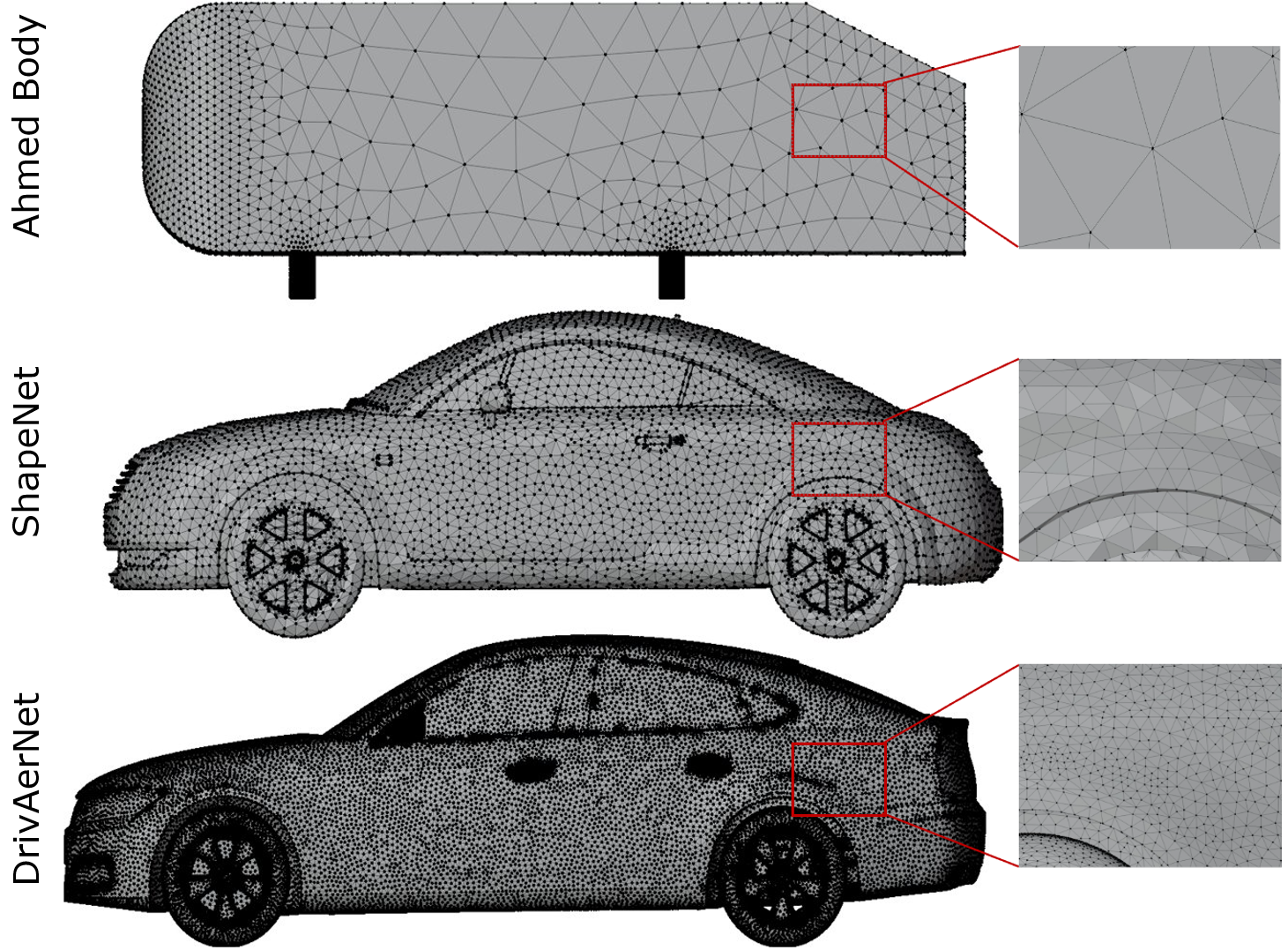
Рис. 3: Mesh resolution comparison across various datasets; first row features the Ahmed body mesh from Li et al. (2023) [22], demonstrating a coarse resolution. Second row shows medium-resolution mesh from the ShapeNet dataset, as utilized by Song et al. (2023) [36]. Final row presents our high-resolution mesh, providing greater detail for in-depth aerodynamic design.

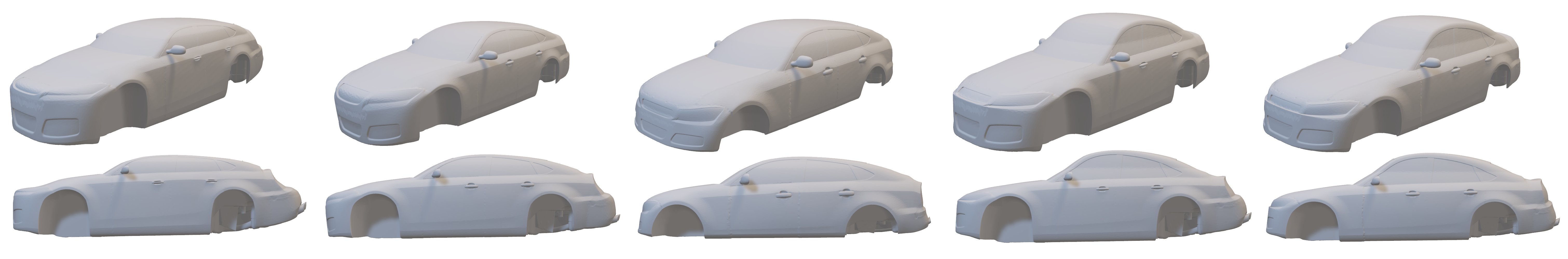
Рис. 4: Car models from the DrivAerNet dataset, illustrating a range of aerodynamic designs. The far left model exhibits the maximum volume within the dataset, while the far right model represents the design with the smallest volume, highlighting the diversity and scope of aerodynamic profiles studied.

Techniques for Generating Diverse Car Designs:

The parametric model, along with the constraints and the bounds applied during the Design of Experiments (DoE), significantly enriches the dataset, making it a robust foundation for the development and training of advanced deep learning models aimed at surrogate modeling and design optimization tasks. We provide access to the parametric model with the incorporated morphing features for further reference and utilization.

Diverging from the approach taken in [19], we implemented a broader range of morphing techniques, enabling us to explore a more diverse array of car designs. This approach aims to enhance the adaptability of deep learning models, allowing them to generalize across various car designs instead of being limited to minor geometric modifications within a single design. Figure 3 depicts the variation in mesh quality, ranging from coarse to high-resolution across various datasets. Our original mesh with 540k mesh faces, provides a denser and more detailed representation compared to the mesh resolutions in the studies by [22] and [36], thereby revealing more detailed geometric and design features.

Additionally, Figure 4 presents a spectrum of car shapes from the DrivAerNet dataset, illustrating the variability in design dimensions and features. This range from the largest to the smallest volume model underscores the dataset’s capacity to cover a comprehensive span of aerodynamic profiles.

3.1 Numerical Simulation

3.1.1 Domain and Boundary Conditions

The DrivAer fastback model scaled 1:1, was selected for conducting the CFD simulations. The simulations were carried out using the open-source software OpenFOAM®, a comprehensive collection of C++ modules for tailoring solvers and utilities in CFD studies. In this study, the coupling between pressure and velocity is achieved through the SIMPLE algorithm (Semi-Implicit Method for Pressure Linked Equations), as implemented in the simpleFoam solver, which is designed for steady-state, turbulent, and incompressible flow simulations. The $k$-$\omega$-SST model, based on Menter’s formulation [24], was chosen for the Reynolds-Averaged Navier-Stokes (RANS) simulations due to its ability to overcome the limitations of the standard $k$-$\omega$ model, particularly its dependency on the freestream values of $k$ and $\omega$, and its effectiveness in predicting flow separation.

The simulations were performed at a flow velocity ($u_{\infty}$) of 30 m/s, which corresponds to a Reynolds number of roughly $9.39\times 10^{6}$, using the car length as the characteristic length scale. The computational mesh is constructed using the SnappyHexMesh (SHM) tool, featuring four distinct refinement zones. Additional layers have been added around the car body to precisely represent wake dynamics and boundary layer evolution (see Figure 2(b)). Boundary conditions were defined with a uniform velocity at the inlet and pressure-based conditions at the outlet. To avoid backflow into the simulation domain, the velocity boundary condition at the outlet was configured as an inletOutlet condition. The car surface and ground were assigned no-slip conditions, while the wheels were modeled to rotate with the rotatingWallVelocity boundary condition. Slip conditions were applied to the lateral and top boundaries of the domain.

Near-wall viscosity effects were addressed using the nutUSpaldingWallFunction wall function approach. The selected wall function for the viscosity term applies a continuous turbulent viscosity profile near the wall, based on velocity, following the approach proposed by [37]. For divergence terms, the default Gauss linear scheme is used, with the velocity convective term discretized using a bounded Gauss linearUpwindV scheme applied to the gradient of velocity, ensuring second-order accuracy. Gradient calculations employed the Gauss linear method complemented by a multi-dimensional limiter to enhance the stability of the solution. The quantities of interest are the 3D velocity field, surface pressure, and wall-shear stresses, as well as the aerodynamic coefficients.

3.1.2 Validation of the Numerical Results

Comparison of Mesh Resolutions and Experimental/Simulation Results
Mesh name	Cell count	DrivAer face count	CPU-hours	Difference Exp.	Difference Ref. Sim.
RANS coarse	$8\times 10^{6}$	$5.4\times 10^{5}$	88	2.81$\%$	1.7$\%$
RANS medium	$16\times 10^{6}$	$5.4\times 10^{5}$	205	0.81$\%$	1.88$\%$
RANS fine	$40\times 10^{6}$	$8.7\times 10^{5}$	512	5.7$\%$	6.78$\%$

Таблица 2: A comparison of different mesh resolutions used in our simulations for the baseline DrivAer model, including cell count and DrivAer face count. The simulation times are listed alongside the percentage differences when compared to experimental results and a referenced simulation, as reported in [17].

The selection of the DrivAer fastback model is justified by the availability of both computational and experimental references, enabling us to benchmark our results against established data [17, 43]. Before commencing the simulations, we conducted a preliminary assessment of how mesh refinement influences the results. This involved comparing the drag coefficients obtained from three different mesh resolutions with experimental values and reference simulation, as detailed in Table 2. The objective was to identify an optimal balance between simulation accuracy and computational efficiency. This balance is crucial since our aim is to generate a large-scale dataset for training deep learning models, necessitating both high fidelity in the simulation results and manageable disk storage and simulation times to accommodate the extensive computational requirements. The drag coefficient, $C_{d}$, is determined by the equation:

$$C_{d}=\frac{F_{d}}{\frac{1}{2}\rho u_{\infty}^{2}A_{\text{ref}}}$$ (1)

The drag force, denoted by $F_{d}$, experienced by a body is a function of its effective frontal area $A_{ref}$, the freestream velocity $u_{\infty}$, and the air density $\rho$. This force comprises both pressure and frictional components.

The evaluation encompassed not only the drag coefficients but also the mesh size and the computational resources required. The simulations were performed on a machine equipped with AMD EPYC 7763 64-Core Processors, totaling 256 CPU cores with 4 Nvidia A100 80GB GPUs.

Our analysis reveals a consistent correlation between our simulations and both the benchmark experimental data and reference simulations, with the 8 and 16 million cell meshes showing particularly good alignment. The discrepancy observed in the 40 million cell mesh could stem from differences in mesh granularity, as the reference simulations utilized a 16 million cell mesh. Finer meshes capture more intricate flow dynamics, which may not be represented in coarser meshes, leading to divergences. In computational fluid dynamics, especially in the preliminary stages of design, an error margin of up to 5$\%$ is generally considered acceptable for engineering purposes. In addition, implementing "RANS fine"for all 4000 designs within the DrivAerNet dataset would require approximately 120TB of storage, posing significant challenges to data sharing and reproducibility due to the immense storage demands. Therefore, considering the balance between accuracy and computational resource allocation, we decided to conduct our simulations using the 8 million and 16 million cell meshes. These configurations provide a compromise between computational efficiency and the level of detail necessary for accurate aerodynamic analysis.

Leveraging Multi-Fidelity Data and Transfer Learning for Efficient Surrogate Model Development:

As shown by [15], leveraging multi-fidelity CFD simulations proves to be a robust strategy for accurate 3D flow field estimation. This approach involves using a dataset that combines RANS, which are relatively easier and cheaper to obtain and can capture the general flow behavior, with Direct Numerical Simulation (DNS) data, known for its detailed flow information despite being computationally expensive. Training a deep learning model with this diverse dataset not only enables the model to generalize effectively to real-world scenarios, as confirmed by wind tunnel tests, but also facilitates a two-phase training process. This process starts with medium-fidelity RANS data to grasp general flow patterns and then transitions to fine-tuning with high-fidelity DNS data, thereby enhancing the model’s accuracy and real-world applicability. Similar results leveraging multi-fidelity datasets for training surrogate models have been demonstrated by [33, 35], underscoring the approach’s efficacy in aerodynamic analysis. The DrivAerNet dataset can be similarly utilized, allowing for integration with datasets of either lower or higher fidelity to augment model training and refine predictive capabilities.

Рис. 5: 3D streamlines representing the magnitude of velocity around the car, alongside the distribution of velocity magnitudes on the car’s wheels. The gradient observed at the wheels is indicative of angular velocity, reflecting the rotation of the wheels. Units are in (m/s).

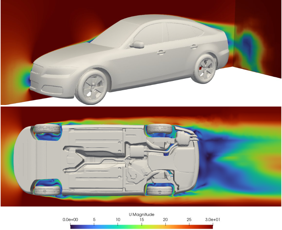
(a) Velocity field distribution around the DrivAer model, with velocity magnitudes expressed in (m/s).

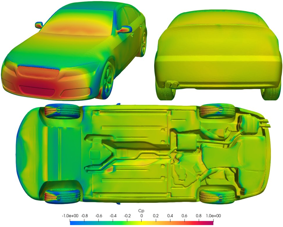
(b) Pressure coefficient ($C_{p}$) distribution on the DrivAer model, illustrating the pressure variation across the car’s surface.

Рис. 6: The DrivAerNet dataset includes detailed 3D fields for velocity, pressure, and wall-shear stresses, alongside aerodynamic coefficients as well as the detailed 3D meshes of the car bodies and both front and rear wheels in each of its entries.

3.1.3 CFD Simulation Results

Inclusion of Diverse Car Dimensions and Complex Flow Dynamics:

In contrast to the approach by [36] where all car models are standardized to a uniform length of 3.5 meters to fit a predefined computational domain, our dataset allows diversity in car dimensions, adjusting the mesh, bounding boxes, and additional layers accordingly for each design. This flexibility is crucial for capturing the intricate flow dynamics around cars including phenomena like flow separation, reattachment, and recirculation zones, and ensuring precise aerodynamic coefficient estimation. This approach addresses limitations observed in some studies that prioritize dataset size over simulation fidelity, often overlooking the importance of convergence, accurate modeling, and appropriate boundary conditions for complex 3D models.

Modeling of Wheels, Side Mirrors, and the Underbody:

As previously highlighted, the majority of literature and available datasets tend to neglect the modeling of wheels, side mirrors, and the underbody, as detailed in Table 1. Our methodology, in contrast, includes detailed modeling of these components. Figure 5 illustrates the velocity distribution on the car: here, the car body exhibits zero velocity due to the no-slip boundary condition, whereas the wheels show nonzero velocity. Additionally, the figure visualizes streamlines around the car, offering insight into the flow dynamics influenced by the inclusion of these features. The DrivAerNet dataset features full 3D flow field information, as shown in Figure 6(a) with the velocity data, and in addition, it provides the pressure distribution on the car’s surface. The pressure coefficient, denoted as $C_{p}$, is calculated as the ratio of the pressure differential $p-p_{\infty}$ to the dynamic pressure, $\frac{1}{2}\rho u^{2}$, and is given by:

$$C_{p}=\frac{p-p_{\infty}}{\frac{1}{2}\rho u^{2}}.$$ (2)

The distribution of $C_{p}$ on the car surface is depicted in Figure 6(b).

3.2 Geometric Feasibility

Ensuring Geometric Integrity in Automated Design Morphing:

In our approach to generating large diverse automotive designs through automated morphing with ANSA®, ensuring the geometric quality and feasibility of each variant is crucial. To address potential issues such as non-watertight geometries, surface intersections, or internal holes resulting from morphing operations, we employ an automated mesh quality assessment and repair process. This procedure not only identifies but also rectifies common geometric anomalies, ensuring that only simulation-ready models are included in our dataset. Geometries failing to meet these criteria are systematically excluded from simulations. The DrivAerNet dataset employs a diverse array of parameters (total of 50 parameters) to morph car geometries, encompassing modifications to the side mirror placement, muffler position, windscreen, rear window length/inclination, the size of the engine undercover, offsets for the doors and fenders, hood positioning, and the scale of headlights as well as alterations to the overall car length and width. Additionally, adjustments are made to the car’s upper and underbody scaling, as well as pivotal angles such as the ramp, diffusor, and trunk lid angles, all crucial for exploring the effects of different design modifications on car aerodynamics. For a detailed account of the morphing parameters, including their lower and upper bounds, please refer to our GitHub repository.

As we morph the entire car’s geometry, wheel positioning is adjusted in the $x$, $y$, and $z$ axes during the morphing process. For all simulations, we use front and rear wheels of the same shape. To accurately simulate the wheel rotation, we export them as separate .stl files post-morphing, which allows us to apply the rotatingWallVelocity physical boundary condition. Moreover, morphing affects the car’s vertical positioning, necessitating a calculation of the $z$-axis displacement to ensure the car body and wheels are properly aligned with the ground plane. For simulation purposes, we supply three distinct .stls: one for the car body, one for the front wheels, and one for the rear wheels, to model their interactions accurately.

3.3 DrivAerNet Dataset Characteristics

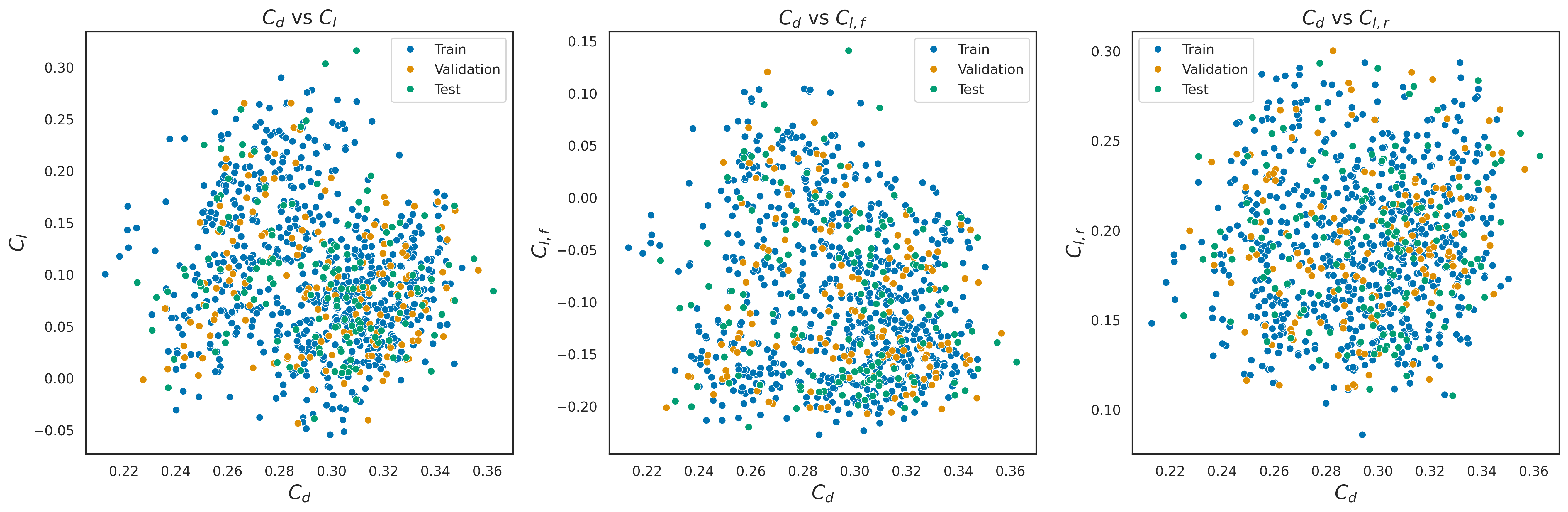
Рис. 7: Scatter plots displaying the relationship between drag coefficient ($C_{d}$) and lift coefficients ($C_{l}$, $C_{l,f}$, $C_{l,r}$) for the DrivAerNet dataset. The dataset represents unique design variants generated via the Optimal Latin Hypercube sampling method, utilizing the Enhanced Stochastic Evolutionary Algorithm (ESE). Data points are categorized into training, validation, and test sets (70$\%$, 15$\%$, 15$\%$).

For our simulations, we employed OpenFOAM® version 11, executing the computational tasks across 128 CPU cores and 4 Nvidia A100 80GB GPUs. This resulted in a total computational cost of approximately 352,000 CPU hours. We make available the complete suite of data, encompassing both the raw CFD outputs and the derived post-processed datasets.

Our dataset serves as a benchmark for evaluating deep learning models, designed to facilitate effective model testing. To manage the large volumes of data from CFD simulations, we employ a data reduction strategy that focuses on key areas of the flow field. This involves retaining data from regions immediately in front of and behind the car, defined within a specific bounding box, which helps to reduce the overall data size significantly. Additionally, we provide a script that converts CFD simulation data into a format suitable for training deep learning models. Given the widespread use of data visualization tools such as ParaView and VisIt, which rely on the Visualization Toolkit (vtk), our dataset is made available in vtk format. This ensures that the data is easily accessible and usable within these common visualization environments, supporting a broad range of research and application needs.

The DrivAerNet dataset offers a comprehensive suite of aerodynamic data pertinent to car geometries, including key metrics such as the total moment coefficient $C_{m}$, the total drag coefficient $C_{d}$, total lift coefficient $C_{l}$, front lift coefficient $C_{l,f}$, and rear lift coefficient $C_{l,r}$. Included within the dataset are crucial parameters like wall-shear stress, and the $y^{+}$ metric, integral for mesh quality evaluations. Further, the dataset provides insights into flow trajectories and detailed cross-sectional analyses of pressure and velocity fields along the $x$ and $y$-axes, enriching the understanding of aerodynamic interactions.

The dataset includes:

• Comprehensive CFD simulation data $\sim$ 16TB

• A curated version of CFD simulations $\sim$ 1TB

• 3D meshes of 4000 car designs and the corresponding aerodynamic performance coefficients ($C_{d}$, $C_{l}$, $C_{l,r}$, $C_{l,f}$, and $C_{m}$) $\sim$ 84GB

• 2D slices include the car’s wake in the $x$-direction and the symmetry plane in the $y$-direction $\sim$ 12GB.

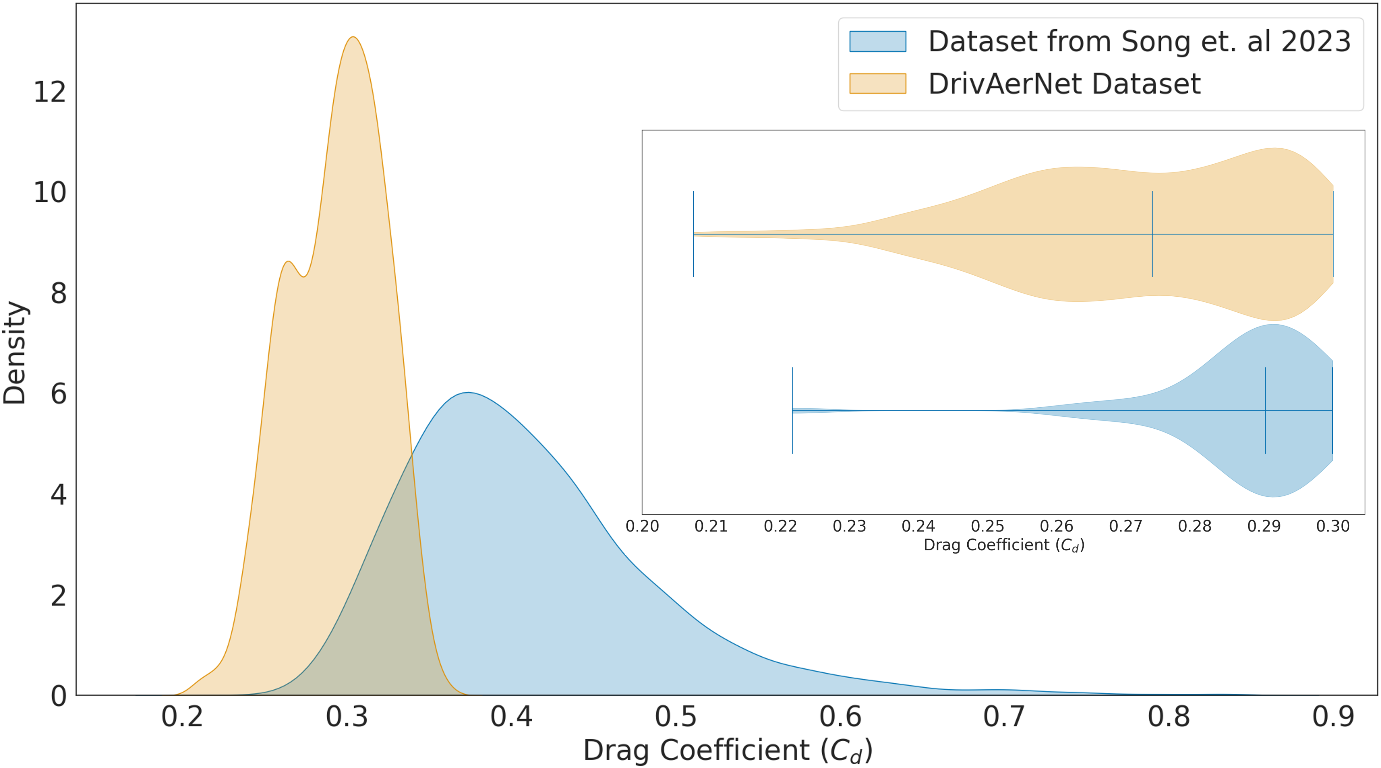
Рис. 8: Comparative Kernel Density Estimation (KDE) and violin plots of drag coefficients from two aerodynamic datasets. The blue curve represents the dataset from Song et. al 2023 [36], and the orange curve corresponds to the DrivAerNet dataset. DrivAerNet focuses on conventional car designs, emphasizing the influence of minor geometric modifications on aerodynamic efficiency.

Aerodynamic Performance Variability Amongst Car Designs in DrivAerNet:

Figure 7 displays three scatter plots that map out the relationships between drag coefficient ($C_{d}$) and various lift coefficients ($C_{l}$, $C_{l,f}$, and $C_{l,r}$) in the DrivAerNet dataset. The data has been split into training, validation, and test sets, with a division of 70$\%$ for training and 15$\%$ each for validation and testing. Such a division is critical for the integrity of the model training process and subsequent performance evaluation.

The Kernel Density Estimation (KDE) plot, illustrated in Figure 8, compares the distribution of drag coefficients across two aerodynamic datasets. Here, we compare the dataset from [36], which spans a broad range of drag values, reflecting a wide variety of car designs in ShapeNet. In contrast, our DrivAerNet dataset targets conventional car designs, accounting for more detailed geometric modifications. This focus is particularly relevant in the context of the engineering design process, where an initial car design is typically refined through incremental changes to optimize aerodynamic performance. The DrivAerNet dataset, therefore, provides a more specific examination of subtle design adjustments and their impact on aerodynamic performance.

In Figure  9, we present the aerodynamic performance across various designs. The top left illustrates the design with lowest drag coefficient $C_{d}$. In contrast, the top right shows the design with the highest $C_{d}$, identifying opportunities for aerodynamic refinement. The bottom left reveals the design with the lowest lift coefficient $C_{l}$ (indicating the largest downforce), which is advantageous for stability at high speeds, while the bottom right exposes design the highest $C_{l}$, potentially complicating aerodynamic stability.

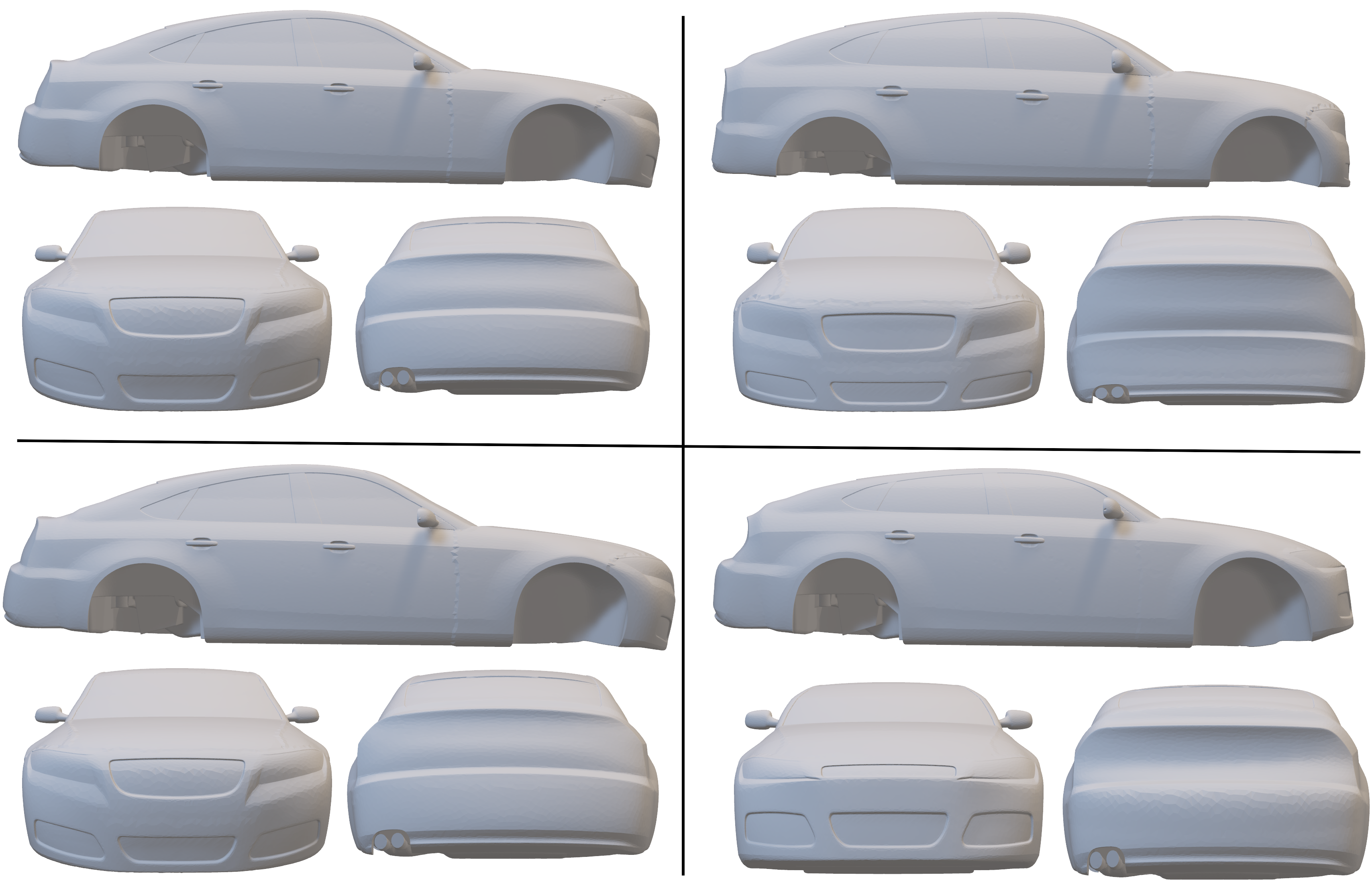
Рис. 9: Aerodynamic performance of car designs from DrivAerNet showcasing a range of coefficients. Top left: Design with minimum drag coefficient $C_{d}$, indicating optimal aerodynamic efficiency. Top right: Design with maximum $C_{d}$. Bottom left: Design with minimum lift coefficient $C_{l}$ (highest downforce). Bottom right: Design with maximum $C_{l}$.

In the next section, we propose a new deep learning method to utilize the dataset for surrogate modeling.

4 Dynamic Graph Convolutional Neural Network for Regression

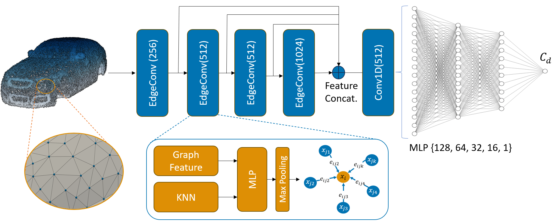
Рис. 10: Architecture of the RegDGCNN for aerodynamic drag prediction. The model processes a 3D mesh by converting it into a point cloud representation. It takes $n$ input points, calculates an edge feature set of size $k$ for each point at an EdgeConv layer, and aggregates features within each set to compute EdgeConv responses for the corresponding points. The output features of the last EdgeConv layer are aggregated globally to form a 1D global descriptor, which is then used to predict the aerodynamic drag coefficient $C_{d}$, enabling direct learning from the 3D geometry of the object. The EdgeConv block ingests an input tensor of dimensions $n\times f$, where it determines edge features for each point utilizing a multi-layer perceptron (MLP). Post-MLP application, the block outputs a tensor of dimensions $n\times a_{n}$ by conducting a pooling operation over the neighboring edge features.

Geometrical deep learning has demonstrated significant promise in addressing fluid dynamics challenges involving irregular geometries, as demonstrated in studies by [34, 26, 1, 20, 32, 30, 29].

In this work, we extend the Dynamic Graph Convolutional Neural Network (DGCNN) framework [42], traditionally associated with PointNet [27] and graph CNN methodologies, to address regression tasks, marking a significant departure from its conventional applications in classification. Our contribution lies in adapting the DGCNN architecture to predict continuous values, specifically focusing on aerodynamic coefficients critical in fluid dynamics and engineering design. Leveraging the spatial encoding capabilities of PointNet and the relational inferences provided by graph CNNs, our proposed RegDGCNN model (as shown in Figure 10) aims to capture the complex interactions of fluid flow around objects, offering a novel method for accurate estimation of crucial aerodynamic parameters. This approach harnesses local geometric structures by constructing a local neighborhood graph and applying convolution-like operations on the edges linking pairs of neighboring points, aligning with graph neural network principles. The technique, termed edge convolution (EdgeConv), is shown to exhibit properties that bridge translation invariance and non-locality. Uniquely, unlike in standard graph CNNs, the graph of RegDGCNN is not static but is dynamically updated after each layer of the network, allowing the graph structure to adapt to evolving feature spaces.

We start by initializing the graph $G$ with node features $X$, along with the parameters for the EdgeConv layers $\theta$ and the Fully Connected (FC) layers $\phi$. A distinctive feature of the RegDGCNN is its dynamic graph construction within each EdgeConv layer, where the $k$-nearest neighbors of each node are identified based on the Euclidean distance in the feature space, thereby adaptively updating the graph’s connectivity to reflect the most significant local structures. The EdgeConv operation is defined as:

$$h_{ij}=\Theta\left(x_{i},x_{j}-x_{i}\right)$$ (3)

enhances node features by aggregating information from these neighbors using a shared Multi-Layer Perceptron (MLP), which processes both the individual node features and their differences with adjacent nodes, capturing the local geometric context effectively.

Following the EdgeConv transformations, global feature aggregation is performed, pooling features from across all nodes into a singular global feature vector:

$$x^{\prime}_{i}=\max_{j\in\mathcal{N}(i)}h_{ij}$$ (4)

Here, max pooling is employed to encapsulate the graph’s holistic information. This global feature vector is subsequently processed through several FC layers, with the inclusion of non-linear activation functions like ReLU and dropout to introduce non-linearity and prevent overfitting, respectively. The architecture culminates in an output layer, designed to suit the specific task at hand, for instance, employing a linear activation for regression tasks.

$$h_{ij}=\text{MLP}\left(\left[x_{i},x_{j}-x_{i}\right]\right)$$ (5)

$$X^{\prime}=\max_{i\in\mathcal{G}}x^{\prime}_{i}$$ (6)

The model’s performance is quantified by calculating the loss between its predicted outputs and the ground truth drag values using the mean squared error (MSE), with the backpropagation algorithm adjusting the model parameters $\theta$ and $\phi$ through optimization algorithms such as Adam [21] to minimize this loss. This iterative refinement process highlights the RegDGCNN’s capability to dynamically leverage and integrate hierarchical features from graph-structured data.

4.1 Implementation Details

Network Architecture:

We constructed the graph for the RegDGCNN using the $k$-nearest neighbors algorithm, with $k$ set to 40. This parameter was critical in defining the local neighborhood over which convolutional operations were performed. The RegDGCNN model was instantiated with specific parameters to accommodate the nature of the regression task. The EdgeConv layers were configured with channels of sizes {256, 512, 512, 1024}, and the following MLP layers were {128, 64, 32, 16}. Lastly, the embedding dimension of the network was set at 512, providing a high-dimensional space to capture the complex features necessary for the regression tasks at hand. Our RegDGCNN model is entirely differentiable and can seamlessly integrate with 3D generative AI applications for enhancing design optimization.

Model Hyperparameters:

The experiments were conducted using the PyTorch framework. The models were trained using a batch size of 32, with the number of points per input set to 5000. Training was distributed across 4 NVIDIA A100 80GB GPUs, utilizing data parallelism to enhance computational efficiency. The network’s learning rate was initially set to 0.001, and a learning rate scheduler was employed to reduce the rate upon plateauing of the validation loss, specifically using the ReduceLROnPlateau scheduler with a patience of 10 epochs and a reduction factor of 0.1. This approach helped in fine-tuning the models by adjusting the learning rate in response to the performance on the validation set. The models were trained for a total of 100 epochs, ensuring sufficient learning while preventing overfitting. For optimization, we used the Adam optimizer [21] due to its adaptive learning rate capabilities.

Inference Time:

The RegDGCNN model, with its compact size of roughly 3 million parameters and a storage requirement of about 10MB, performs drag estimation for a car design with 540k mesh faces in 1.2 seconds on 4 A100 80GB GPUs, a significant efficiency gain compared to the 2.3 hours taken by a standard CFD simulation on 128 CPU cores with 4 A100 80GB GPUs.

5 Surrogate Modeling of Aerodynamic Drag

In this section, we evaluate our RegDGCNN model on two aerodynamic datasets, DrivAerNet and ShapeNet, highlight the impact of larger training volumes on model performance, and investigate the model’s learned features.

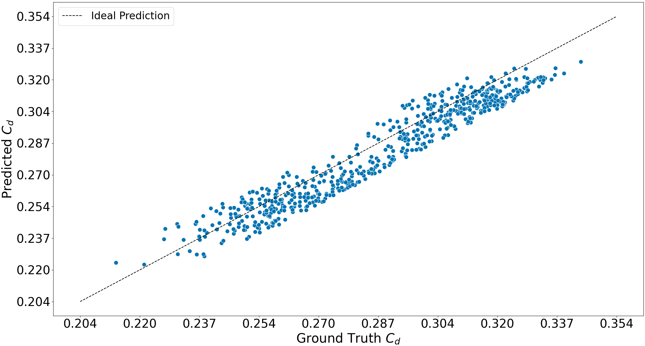
Рис. 11: Correlation plot of the predicted drag coefficient $C_{d}$ by our RegDGCNN model against the ground truth for the DrivAerNet unseen test set, achieving an $R^{2}$ score of 0.9. The dotted line denotes the line of perfect correlation, representing the ideal prediction scenario.

5.1 DrivAerNet: Aerodynamic Drag Prediction of High-Resolution Meshes

The examination of RegDGCNN’s performance on the DrivAerNet dataset, depicted in Figure 11, reveals a good correlation between predicted values and ground-truth data from CFD, underscoring the model’s effectiveness. The complexity of the DrivAerNet dataset is attributed to its inclusion of industry-standard shapes, varied through 50 geometric parameters, presenting a comprehensive challenge in aerodynamic prediction. Our model effectively navigated the complexities of the dataset and directly processed the 3D mesh data, marking a significant shift from traditional methods that often rely on generating Signed Distance Fields (SDF) or rendering 2D images. This straightforward approach enabled us to achieve an $R^{2}$ score of 0.9 on the unseen test set, emphasizing the model’s ability to accurately discern subtle aerodynamic differences.

5.2 ShapeNet: Aerodynamic Drag Prediction of Arbitrary Vehicle Shapes

To test the generalizability of the proposed RegDGCNN model, we also evaluated its ability to adapt to complex geometries on an existing benchmark dataset, utilizing 2,479 diverse car designs from the ShapeNet dataset [36] (see Figure 12), which exhibits a broader range of car shapes than our DrivAerNet dataset.

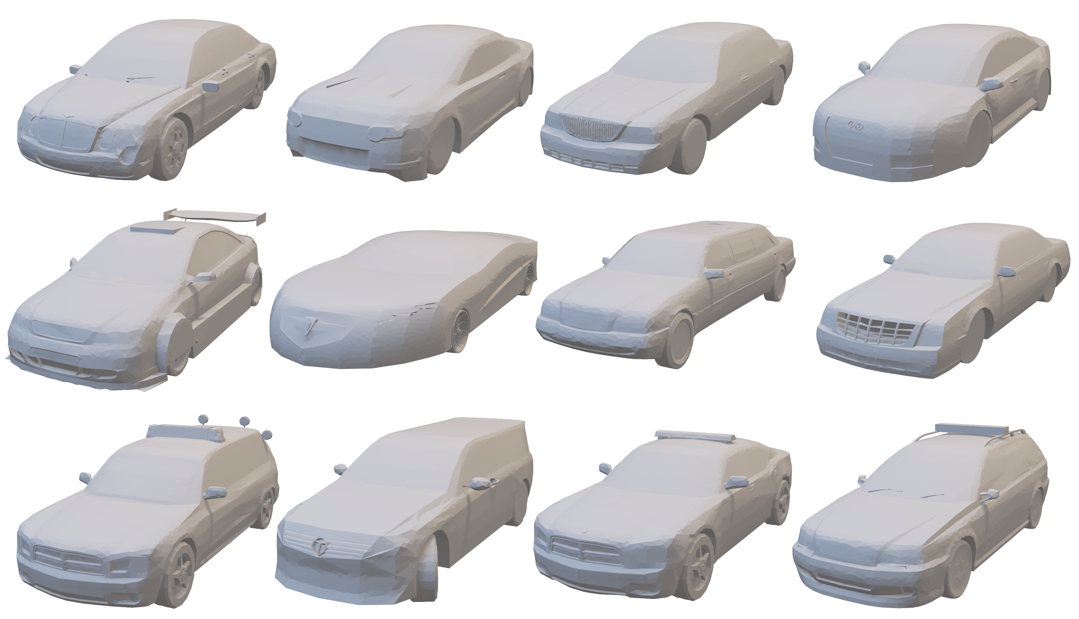
Рис. 12: A selection of car samples from the ShapeNet dataset, demonstrating the diversity in car shapes and mesh resolutions, utilized to evaluate the generalization capabilities of RegDGCNN. These samples provide a comparative baseline against the high-resolution meshes found in our DrivAerNet dataset.

In Table 3, we compare the performance of two models: the attn-ResNeXt model from the study by [36], which implements a self-attention mechanism to boost the understanding of interactions among various regions of an image. It uses 2D depth/normal renderings as input and has approximately 2 billion parameters, achieving an $R^{2}$ score of 0.84; our proposed RegDGCNN model, which directly processes 3D mesh data, significantly reduces the number of parameters to 3 million, and achieves a superior $R^{2}$ score of 0.87. This comparison underscores the efficiency and effectiveness of our model in aerodynamic drag prediction tasks.

Таблица 3: Comparison of model performance for drag prediction on arbitrary car shapes from the ShapeNet dataset.

Model	Input	$R^{2}$	$\#$ Parameters
attn-ResNeXt [36]	2D Depth/Normal Renderings	0.84	2B
RegDGCNN (ours)	3D Mesh	0.87	3M

5.3 Effect of Training Dataset Size

For both ShapeNet and DrivAerNet datasets, we first allocated 70$\%$ for training, and 15$\%$ each for validation and testing. Subsequently, we experimented with training subsets at 20$\%$, 40$\%$, 60$\%$, 80$\%$, and 100$\%$ of the training portion. The ShapeNet subsets ranged from 1270 to 6352 samples. Meanwhile, for the DrivAerNet dataset, the corresponding sample sizes were 560, 1120, 1680, 2240, and 2800 samples.

Figure 13 reveals a clear trend where the average relative error in drag coefficient predictions decreases as the percentage of the dataset used for training increases. This trend is consistent for both datasets, underscoring the common machine learning principle that more training data generally leads to better model performance. The improved performance of the DrivAerNet Dataset across all sizes of training data highlights the critical role of bigger datasets in machine learning models for aerodynamics and further establishes the value of DrivAerNet dataset, which is significantly larger than previous open-source datasets.

The figure also indicates that RegDGCNN yields better performance on the DrivAerNet dataset compared to the dataset from ShapeNet. This can be attributed to several factors:

• The large variation in shapes within ShapeNet does not correspond with an adequate number of samples to encompass the entire range of aerodynamic drag values.

• ShapeNet models cars were modeled as single-bodied entities, omitting crucial details like wheels and underbodies that are vital for accurate aerodynamic modeling.

• All drag values in ShapeNet were computed using a single reference area, which does not account for the significant variation in frontal projected areas of different car designs.

• There is a considerable variation in mesh resolutions across the ShapeNet dataset, potentially leading to inconsistencies in aerodynamic predictions.

This analysis serves to demonstrate the generalization capabilities of our model, emphasizing the objective of developing models that effectively generalize to out-of-domain distributions.

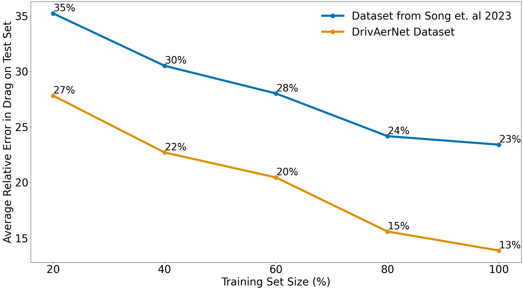
Рис. 13: Average relative error in drag coefficient predictions on the unseen test set for our model RegDGCNN, based on training set size. The results from the ShapeNet drag dataset [36] are denoted in blue, while results from the DrivAerNet dataset are shown in orange. The training set sizes vary from 20$\%$ to 100$\%$. We observe that the increase in dataset size leads to significant error reduction, showing the necessity of larger datasets in aerodynamic surrogate modeling.

5.4 Features Learned

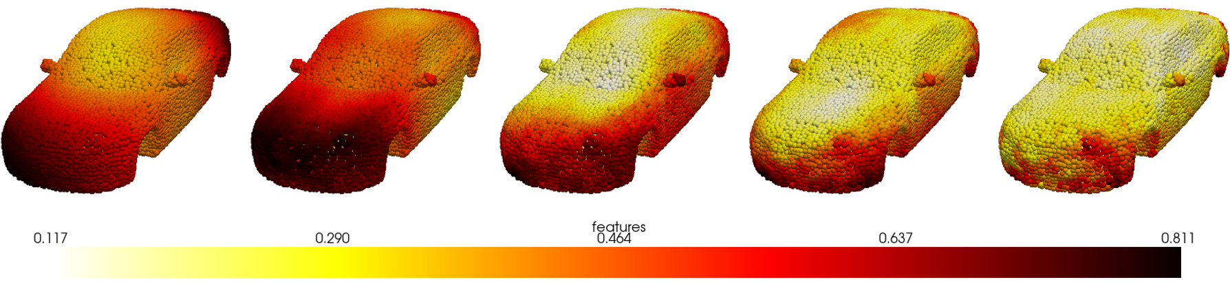
Рис. 14: Visualization of feature importance across an upsampled point cloud of a car model from DrivAerNet, derived from our RegDGCNN, specifically focusing on features from the EdgeConv layers. Feature intensities are color-coded from low (light yellow) to high (dark red), indicating areas of significant learning focus by the convolutional layers. This mapping highlights the learned features that contribute to the model’s predictions.

To further assess the model’s performance, we analyze the features learned in the intermediate layers following the edge convolution operations. Figure 14 illustrates the distribution of feature importance across an upsampled point cloud of a car sample from DrivAerNet, with color coding from light yellow (low importance) to dark red (high importance). Initially, RegDGCNN zeroes in on the car’s frontal and rear area, which are critical in shaping aerodynamic performance. This focus is notably pertinent for aerodynamic design, as the frontal area has a substantial effect on pressure drag and the rear area is particularly relevant due to its role in airflow separation and wake region formation. As the model delves deeper through its layers, it starts to recognize more complex geometric details. Conversely, areas such as the roof and windows are less crucial for drag, underscoring the model’s adeptness at identifying areas with a more significant aerodynamic influence.

6 Limitations and Future Work

This section discusses the limitations of our study. Despite careful selection to ensure a balance between detail and computational efficiency, the model’s parameterization faces an inherent limitation. This stems from the trade-off between the compactness of the representation and the flexibility needed to capture a broad range of aerodynamic phenomena. Consequently, while our approach offers valuable insights for many applications, it may not fully encompass all aerodynamic variabilities pertinent to automotive engineering. The dataset comprises 4,000 instances, which, while significant, might not fully capture the broad spectrum of real-world automotive designs. Additionally, our focus was primarily on drag prediction; however, we plan to extend the application of RegDGCNN to include surface field predictions in future work. While our dataset is large and of high-fidelity, it is important to acknowledge that we are still in the early stages of approaching the scale and foundational impact seen in AI fields like image processing and natural language processing, where large datasets are a norm.

One of the key challenges in applying graph-based methods like RegDGCNN is the significant GPU memory requirements. This is due to the need to compute all pairwise distances between points, which can be highly memory-intensive. Moreover, the non-uniform density of point clouds introduces additional complexities; a fixed $k$-nearest neighbors approach may not be suitable for areas with varying densities of points.

Another limitation is that, in its current form, RegDGCNN does not reduce the number of points during the forward pass for large-scale point clouds, leading to high computational demands and potentially limiting the model’s scalability to even larger datasets. Addressing these challenges will be crucial for advancing the capabilities and applications of graph-based neural networks in processing complex aerodynamic data.

7 Conclusion

In our conclusion, we highlight the distinct advantages of DrivAerNet, which, by focusing on detailed geometric modifications, outperforms broader datasets such as those referenced in [36, 22, 31], especially in the context of real-world aerodynamic design applications. Additionally, the compact RegDGCNN model, with 3 million parameters and 10MB size, efficiently estimates drag in just 1.2 seconds for industry-standard designs with 540k mesh faces, significantly outpacing traditional CFD simulations. Moreover, our RegDGCNN model, in particular, showcases superior performance by directly processing 3D meshes, thereby eliminating the need for 2D image rendering or the generation of Signed Distance Functions (SDF), which simplifies the preprocessing stages and increases the model’s accessibility. Importantly, the RegDGCNN model’s ability to deliver precise drag predictions without requiring water-tight meshes highlights its adaptability and effectiveness in leveraging real-world data. Through the expansion of the DrivAerNet dataset from 560 to 2800 samples, we achieved a remarkable reduction in error by approximately 75$\%$. Similarly, on the dataset from [36], increasing the training samples from 1270 to 6352 led to a 56$\%$ decrease in error, underscoring the substantial impact of dataset scale on enhancing the performance of deep learning models in aerodynamic studies. The inclusion of specific parametric alterations (50 geometric parameters) within our DrivAerNet dataset has significantly improved model learning, resulting in a notable increase in predictive accuracy, essential for the refinement of aerodynamic designs. This emphasizes the critical role of large detailed, high-fidelity datasets in crafting models capable of adeptly handling the complexities inherent in aerodynamic surrogate modeling.

8 Acknowledgements

The research work of Mohamed Elrefaie was supported by the German Academic Exchange Service (DAAD) under the IFI - "Internationale Forschungsaufenthalte für Informatikerinnen und Informatiker"Grant and the Department of Mechanical Engineering at MIT. The authors thank Florin Morar from BETA CAE Systems USA Inc for his support with morphing the DrivAer model in ANSA®. We extend our gratitude to Christian Breitsamter for his role in facilitating the organizational aspects of this research.

- [1] A. Abbas, A. Rafiee, M. Haase, and A. Malcolm. Geometrical deep learning for performance prediction of high-speed craft. Ocean Engineering, 258:111716, 2022.
- [2] S. R. Ahmed, G. Ramm, and G. Faltin. Some salient features of the time -averaged ground vehicle wake. SAE Transactions, 93:473–503, 1984.
- [3] N. Arechiga, F. Permenter, B. Song, and C. Yuan. Drag-guided diffusion models for vehicle image generation. arXiv preprint arXiv:2306.09935, 6 2023.
- [4] N. Ashton, P. Batten, A. Cary, and K. Holst. Summary of the 4th high-lift prediction workshop hybrid rans/les technology focus group. Journal of Aircraft, pages 1–30, 2023.
- [5] N. Ashton and W. van Noordt. Overview and summary of the first automotive cfd prediction workshop: Drivaer model. SAE International Journal of Commercial Vehicles, 16(02-16-01-0005), 2022.
- [6] M. Aultman, Z. Wang, R. Auza-Gutierrez, and L. Duan. Evaluation of cfd methodologies for prediction of flows around simplified and complex automotive models. Computers & Fluids, 236:105297, 2022.
- [7] P. Baque, E. Remelli, F. Fleuret, and P. Fua. Geodesic convolutional shape optimization. In J. Dy and A. Krause, editors, Proceedings of the 35th International Conference on Machine Learning, volume 80 of Proceedings of Machine Learning Research, pages 472–481. PMLR, 10–15 Jul 2018.
- [8] F. Bonnet, J. Mazari, P. Cinnella, and P. Gallinari. Airfrans: High fidelity computational fluid dynamics dataset for approximating reynolds-averaged navier–stokes solutions. Advances in Neural Information Processing Systems, 35:23463–23478, 2022.
- [9] C. Brand, J. Anable, I. Ketsopoulou, and J. Watson. Road to zero or road to nowhere? disrupting transport and energy in a zero carbon world. Energy Policy, 139:111334, 2020.
- [10] A. X. Chang, T. Funkhouser, L. Guibas, P. Hanrahan, Q. Huang, Z. Li, S. Savarese, M. Savva, S. Song, H. Su, et al. Shapenet: An information-rich 3d model repository. arXiv preprint arXiv:1512.03012, 2015.
- [11] A. Cogotti. A parametric study on the ground effect of a simplified car model. SAE transactions, pages 180–204, 1998.
- [12] G. Damblin, M. Couplet, and B. Iooss. Numerical studies of space-filling designs: optimization of latin hypercube samples and subprojection properties. Journal of Simulation, 7(4):276–289, 2013.
- [13] J. Deng, W. Dong, R. Socher, L.-J. Li, K. Li, and L. Fei-Fei. Imagenet: A large-scale hierarchical image database. In 2009 IEEE conference on computer vision and pattern recognition, pages 248–255. Ieee, 2009.
- [14] M. Elrefaie, T. Ayman, M. A. Elrefaie, E. Sayed, M. Ayyad, and M. M. AbdelRahman. Surrogate modeling of the aerodynamic performance for airfoils in transonic regime. In AIAA SCITECH 2024 Forum, page 2220, 2024.
- [15] M. Elrefaie, S. Hüttig, M. Gladkova, T. Gericke, D. Cremers, and C. Breitsamter. Real-time and on-site aerodynamics using stereoscopic piv and deep optical flow learning. arXiv preprint arXiv:2401.09932, 2024.
- [16] E. Gunpinar, U. C. Coskun, M. Ozsipahi, and S. Gunpinar. A generative design and drag coefficient prediction system for sedan car side silhouettes based on computational fluid dynamics. CAD Computer Aided Design, 111:65–79, 6 2019.
- [17] A. I. Heft, T. Indinger, and N. A. Adams. Experimental and numerical investigation of the drivaer model. In Fluids Engineering Division Summer Meeting, volume 44755, pages 41–51. American Society of Mechanical Engineers, 2012.
- [18] A. I. Heft, T. Indinger, and N. A. Adams. Introduction of a new realistic generic car model for aerodynamic investigations. Technical report, SAE Technical Paper, 2012.
- [19] S. J. Jacob, M. Mrosek, C. Othmer, and H. Köstler. Deep learning for real-time aerodynamic evaluations of arbitrary vehicle shapes. SAE International Journal of Passenger Vehicle Systems, 15(2):77–90, mar 2022.
- [20] A. Kashefi and T. Mukerji. Physics-informed pointnet: A deep learning solver for steady-state incompressible flows and thermal fields on multiple sets of irregular geometries. Journal of Computational Physics, 468:111510, 2022.
- [21] D. P. Kingma and J. Ba. Adam: A method for stochastic optimization. arXiv preprint arXiv:1412.6980, 2014.
- [22] Z. Li, N. B. Kovachki, C. Choy, B. Li, J. Kossaifi, S. P. Otta, M. A. Nabian, M. Stadler, C. Hundt, K. Azizzadenesheli, and A. Anandkumar. Geometry-informed neural operator for large-scale 3d pdes, 2023.
- [23] H. Martins, C. Henriques, J. Figueira, C. Silva, and A. Costa. Assessing policy interventions to stimulate the transition of electric vehicle technology in the european union. Socio-Economic Planning Sciences, 87:101505, 2023.
- [24] F. R. Menter, M. Kuntz, R. Langtry, et al. Ten years of industrial experience with the sst turbulence model. Turbulence, heat and mass transfer, 4(1):625–632, 2003.
- [25] P. Mock and S. Díaz. Pathways to decarbonization: the european passenger car market in the years 2021–2035. communications, 49:847129–848102, 2021.
- [26] T. Pfaff, M. Fortunato, A. Sanchez-Gonzalez, and P. W. Battaglia. Learning mesh-based simulation with graph networks. arXiv preprint arXiv:2010.03409, 2020.
- [27] C. R. Qi, H. Su, K. Mo, and L. J. Guibas. Pointnet: Deep learning on point sets for 3d classification and segmentation. In Proceedings of the IEEE conference on computer vision and pattern recognition, pages 652–660, 2017.
- [28] E. Remelli, A. Lukoianov, S. Richter, B. Guillard, T. Bagautdinov, P. Baque, and P. Fua. Meshsdf: Differentiable iso-surface extraction. Advances in Neural Information Processing Systems, 33:22468–22478, 2020.
- [29] T. Rios, B. Sendhoff, S. Menzel, T. Back, and B. V. Stein. On the efficiency of a point cloud autoencoder as a geometric representation for shape optimization. pages 791–798. Institute of Electrical and Electronics Engineers Inc., 12 2019.
- [30] T. Rios, B. V. Stein, T. Back, B. Sendhoff, and S. Menzel. Point2ffd: Learning shape representations of simulation-ready 3d models for engineering design optimization. pages 1024–1033. Institute of Electrical and Electronics Engineers Inc., 2021.
- [31] T. Rios, B. van Stein, P. Wollstadt, T. Bäck, B. Sendhoff, and S. Menzel. Exploiting local geometric features in vehicle design optimization with 3d point cloud autoencoders. In 2021 IEEE Congress on Evolutionary Computation (CEC), pages 514–521, 2021.
- [32] T. Rios, P. Wollstadt, B. V. Stein, T. Back, Z. Xu, B. Sendhoff, and S. Menzel. Scalability of learning tasks on 3d cae models using point cloud autoencoders. pages 1367–1374. Institute of Electrical and Electronics Engineers Inc., 12 2019.
- [33] F. Romor, M. Tezzele, M. Mrosek, C. Othmer, and G. Rozza. Multi-fidelity data fusion through parameter space reduction with applications to automotive engineering. International Journal for Numerical Methods in Engineering, 124(23):5293–5311, 2023.
- [34] A. Sanchez-Gonzalez, J. Godwin, T. Pfaff, R. Ying, J. Leskovec, and P. Battaglia. Learning to simulate complex physics with graph networks. In International conference on machine learning, pages 8459–8468. PMLR, 2020.
- [35] Y. Shen, H. C. Patel, Z. Xu, and J. J. Alonso. Application of multi-fidelity transfer learning with autoencoders for efficient construction of surrogate models. In AIAA SCITECH 2024 Forum, page 0013, 2024.
- [36] B. Song, C. Yuan, F. Permenter, N. Arechiga, and F. Ahmed. Surrogate modeling of car drag coefficient with depth and normal renderings. arXiv preprint arXiv:2306.06110, 2023.
- [37] D. B. Spalding. The numerical computation of turbulent flow. Comp. Methods Appl. Mech. Eng., 3:269, 1974.
- [38] N. Thuerey, K. Weißenow, L. Prantl, and X. Hu. Deep learning methods for reynolds-averaged navier–stokes simulations of airfoil flows. AIAA Journal, 58(1):25–36, 2020.
- [39] T. L. Trinh, F. Chen, T. Nanri, and K. Akasaka. 3d super-resolution model for vehicle flow field enrichment. In Proceedings of the IEEE/CVF Winter Conference on Applications of Computer Vision, pages 5826–5835, 2024.
- [40] N. Umetani and B. Bickel. Learning three-dimensional flow for interactive aerodynamic design. ACM Transactions on Graphics, 37, 2018.
- [41] M. Usama, A. Arif, F. Haris, S. Khan, S. K. Afaq, and S. Rashid. A data-driven interactive system for aerodynamic and user-centred generative vehicle design. In 2021 International Conference on Artificial Intelligence (ICAI), pages 119–127, 2021.
- [42] Y. Wang, Y. Sun, Z. Liu, S. E. Sarma, M. M. Bronstein, and J. M. Solomon. Dynamic graph cnn for learning on point clouds. ACM Transactions on Graphics (tog), 38(5):1–12, 2019.
- [43] D. Wieser, H.-J. Schmidt, S. Mueller, C. Strangfeld, C. Nayeri, and C. Paschereit. Experimental comparison of the aerodynamic behavior of fastback and notchback drivaer models. SAE International Journal of Passenger Cars-Mechanical Systems, 7(2014-01-0613):682–691, 2014.