Experimental demonstration of the shadow of a laser beam

Abstract

Light, being massless, casts no shadow; under ordinary circumstances, photons pass right through each other unimpeded. Here, we demonstrate a laser beam acting like an object – the beam casts a shadow upon a surface when the beam is illuminated by another light source. We observe a regular shadow in the sense it can be seen by the naked eye, it follows the contours of the surface it falls on, and it follows the position and shape of the object (the laser beam). Specifically, we use a nonlinear optical process involving four atomic levels of ruby. We are able to control the intensity of a transmitted laser beam by applying another perpendicular laser beam. We experimentally measure the dependence of the contrast of the shadow on the power of the object laser beam, finding a maximum of approximately of approximately 22%, similar to that of a shadow of a tree on a sunny day. We provide a theoretical model that predicts the contrast of the shadow. Making light itself cast a shadow opens new possibilities for fabrication, imaging, and illumination.

Human’s physical understanding of shadows developed hand-in-hand with our understanding of light and optics. Throughout this multi-millennia history, humans saw that shadows were cast by material objects like trees, clouds, or the Moon. The study and use of shadows runs through the history of arts and science. In theatre, shadow puppetry has existed for millennia in various cultures around the world. In fine art, the Renaissance investigation of shadows, e.g., by Leonardo da Vinci and Dürer, contributed to the development of perspective and realism in Western painting. In astronomy, shadows revealed our relation to the cosmos; the discovery that eclipses are shadows led to the measurement of the sizes and distances of the Moon and the Sun, while Eratosthenes used shadows to measure the circumference of the Earth.

In optics, Ibn Al-Haytham’s description of shadows lent credibility to the ray model of light, while Grimaldi, Fresnel, and Arago’s detailed observations of and predictions for shadows introduced the concept of diffraction and the wave model. In mathematics, the understanding that shadows are projections (i.e., silhouettes) of an object led to early mapping-projections and seeded key concepts in linear algebra. In philosophy, one of the most well-known texts is Plato’s allegory of the cave, a discussion based on shadows. In technology, shadows are the basis of contact-lithography, X-ray images, and a plethora of ways to measure and reconstruct three-dimensional objects, e.g., computer-aided tomography. Over the century-spanning course of this study, a shadow has come to be defined as a dark area on a surface where light has been blocked by an object. All along, regardless of whether the object is solid, gaseous, or liquid, or whether it is opaque or translucent, it has been implicitly assumed that it is material, i.e., made of some object with mass.

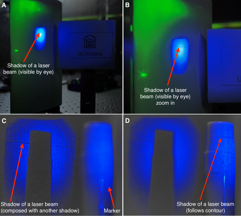
Figure 1: Photographic images of the shadow of a laser beam. A high-power green laser beam (the object), travelling through a cube of ruby, is illuminated from the side by blue light.  (A) A photograph of the shadow cast by the object laser beam on a piece of white paper, image magnified approximately by a factor of 4 using a simple lens. Hence, regardless of magnified or not, it portrays what can be seen in person. (B) A zoom in version of (A). A white plastic marker (i.e., a broad tip pen) is placed in the path of the shadow, between the object beam and the paper, and the camera focus is fixed on (C) the paper or (D) the marker, thereby showing that the shadow follows the contours of the surface the shadow falls on. All images were taken with a regular consumer digital camera in a darkened room.

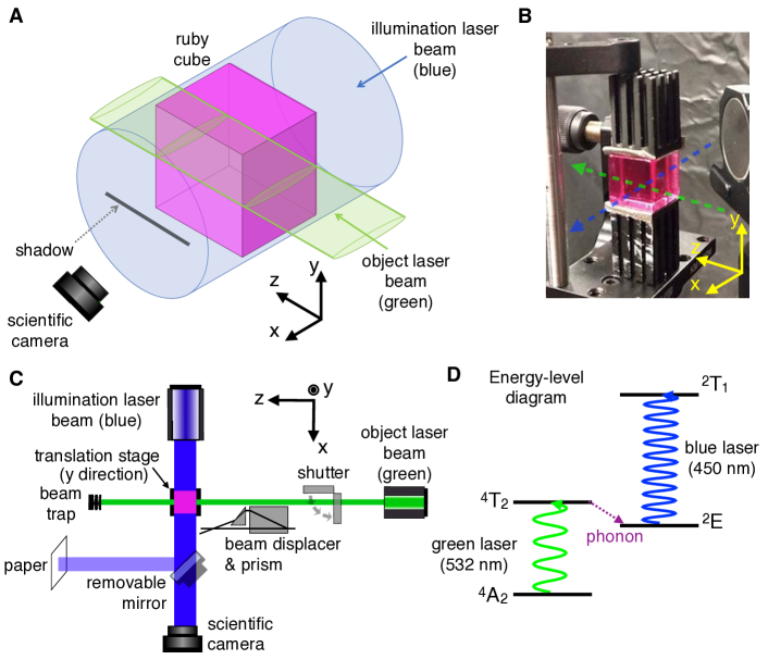
Figure 2: Scheme to create and observe the laser shadow. (A) The object laser beam (green) travels through a ruby cube and casts a shadow in the illuminating blue light. (B) A photograph of the ruby cube overlayed with the beam directions. (C) The simplified experimental setup to observe the shadow cast either on paper or, for quantitative measurements, impinging directly on the camera. (D) The relevant energy level diagram of ruby. As described in detail in the Theory Section, a photon from the green laser beam excites the lower transition, which then causes electrons to populate the ${}^{2}\text{E}$ energy level, and consequently increases the absorption (i.e., blocks) of the blue (illumination) light.

We demonstrate a counter-example to that, a shadow cast by a massless object, light itself. The shadow we observe is not some clever scientific analogy, nor a subtle technical effect, but rather a genuine shadow that has the usual characteristics of a typical shadow created by a material object. Namely, the shadow fulfills the criteria: (i) it is a large-scale effect that is (ii) visible by eye on ordinary surfaces. Moreover, (iii) it is due to the object blocking the illumination light and, thus, (iv) it takes the shape of the illuminated object and (v) follows as the object changes position or shape. Lastly, (vi) the shadow follows the contour of the object it falls on, giving the sense of three-dimensionality (3D) that interested da Vinci and creating an effect that is often used for depth measurement in the 3D imaging of scenes by cameras.

As our immaterial object we use a laser beam, namely a high-power green beam with an optical wavelength of 532 nm. This object beam travels through a cube of standard ruby crystal. We illuminate the beam from the side with blue light. We start with qualitative observations. Fig. 1 (A) shows the shadow of the object beam cast on a piece of paper. The laser shadow extends through an entire face of the rube cube, about 1.2 cm long, confirming the macroscopic scale, criteria (i). Moreover, Fig. 1 (A) is a photo taken with a consumer photography camera. It genuinely portrays what can be seen in person, criteria (ii). Fig. 1 (C) and (D) show the shadow falling across a marker made from white plastic that is placed in front of the paper. Just as one would expect, the shadow follows the depth-contours of the scene: the rounded surface of the marker and the flat paper behind it, thereby confirming criteria (vi). Thus, three of the six criteria have been qualitatively confirmed.

In the next section, we propose a physical model for the mechanism in the ruby that underlies the laser shadow effect. We present a comparison of the quantitative predictions of the model with measurements of the shadow’s shape and contrast. We then return to the remaining two criteria and provide evidence that they too are satisfied by the laser shadow effect.

We emphasize that under ordinary circumstances, photons do not interact with each other. However, photon-photon interaction can happen under special cases. For example, in the Hong–Ou–Mandel effect, one can observe photon bunching HOM_effect ; bouchard_HOM_review_2020 ; PRA_Jordan2022 . In the presence of a nonlinear medium boyd_nonlinear , photons can interact through Rydberg mediated photon-photon interaction Rydberg1 ; Rydberg2 ; Rydberg3 . Although not yet observed, photon-photon interaction are studied in the context of vacuum polarization scattering_vacuum_1 ; scattering_vacuum_2 ; scattering_vacuum_3 ; scattering_vacuum_4 ; scattering_vacuum_5 . We highlight that the effect we are reporting does not fall in any of these categories.

I Theory

In order to observe the shadow of a laser beam, one requires a medium that exhibits a strong nonlinear absorption. However, most materials exhibit saturation of absorption at high laser intensities meaning that the material becomes more transparent in the presence of a strong laser field. This would lead to an “anti-shadow” where the shadow location of the laser beam appears brighter than the background.

However, some materials can exhibit an increase in absorption at higher intensities under certain conditions. This response is known as reverse saturation of absorption and requires particular conditions which includes a more than two-level system. Moreover, the excited state must have a larger absorption cross-section than the ground state. In addition, neither the first nor the second excited states should decay to other levels that can trap the atomic population. Furthermore, the incident light should saturate the first transition only. A recent study shows that ruby satisfies all these conditions and exhibits reverse-saturation of absorption Safari_arxiv2023 .

The laser shadow effect is conceptually depicted in Fig. 2 (A)–(D), where we show the propagating paths of the object laser beam (green) and the illumination laser beam (blue). The laser shadow effect is a consequence of the optical nonlinear absorption (i.e., reverse-saturation of absorption, equivalently called saturable transmission) in the ruby; wherever the object laser beam (green) exists in the ruby, it increases the optical absorption of the illuminating laser (blue). This results in a matching region in the illuminating light with lower optical intensity, a darker area that is the shadow of the green laser beam.

At a fundamental level, this effect is explained by the atomic structure of the ruby and its optical properties boyd_nonlinear ; boyd_gaeta2008 ; bigelow2003superluminal ; gehring2006observation ; kramer1986nonlinear ; bigelow2003observation ; franke2011rotary ; cronemeyer1966optical ; Maiman_PRL_1960 ; maiman1960stimulatedNature ; boyd_gauthier2002 ; boyd2009controlling ; Kiang1965 . Ruby (Al2O3:Cr) is an aluminium oxide crystal and the distinct ruby-red colour comes from chromium impurities (i.e., atoms) that distort the crystal lattice. The relevant energy levels of the ruby crystal lattice presented in the diagram in Fig. 2 (D) exhibit an unusual interaction, that we will now describe, between select colours of light. One colour is green, the object laser beam, which has an optical wavelength of 532 nm. It will drive the transition from the ground state ${}^{4}\text{A}_{2}$ to an excited state ${}^{4}\text{T}_{2}$, which then decays rapidly via phonons to the ${}^{2}\text{E}$ state. This then allows the electrons to absorb blue light (450 nm), the illumination, by transitioning from ${}^{2}\text{E}$ to ${}^{2}\text{T}_{1}$. However, the blue laser (450 nm) could in principle be absorbed by the electrons in ${}^{4}\text{A}_{2}$ and transition to some other level (not shown in the diagram). The effect will only take place if the absorption cross-section of the second transition (${}^{2}\text{E}$ to ${}^{2}\text{T}_{1}$) is larger than the one of the first transition (${}^{4}\text{A}_{2}$ to ${}^{4}\text{T}_{2}$), which is the special case exhibited by ruby.

Two comments about the observation of the laser shadow effect need to be made explicitly. First, both lasers, the green and blue, are not on resonance to each other, as this is not required to achieved the effect. Second, the blue laser transition does not cycle. These two aspects make it simpler to use and explore the laser shadow effect.

In the Supplementary Material, we present the analytical rate equations that model these transitions and, thus, model the laser shadow effect. This model shows that the contrast between the shadow and its surrounding illumination increases monotonically with optical power of the green laser and that the shape of the shadow follows the spatial intensity profile of the green laser beam. In the next section, we present our quantitative analysis of the laser shadow effect and the comparison between measurements and the model.

II Experiment and Results

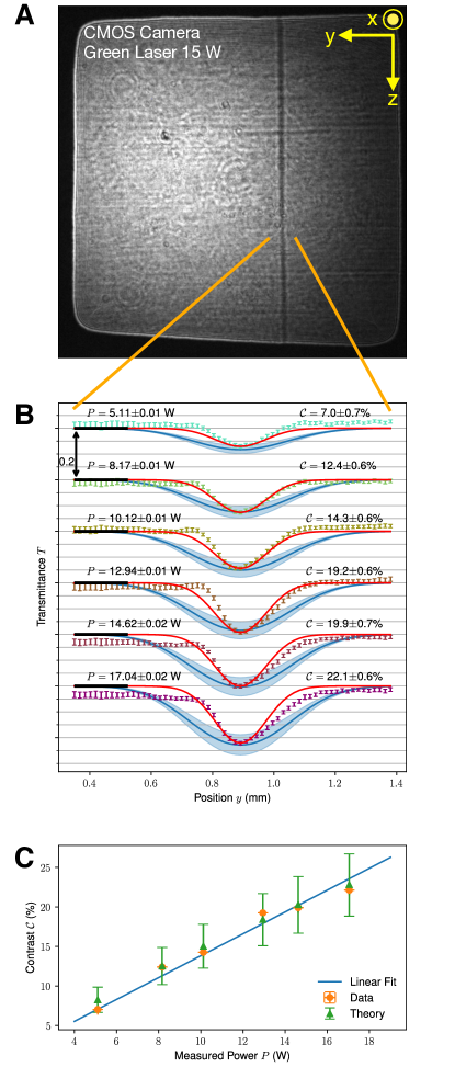
Figure 3: Quantitative analysis of the shadow contrast. (A) Direct image of the illuminating light transmitted through the ruby for a 15 W object laser beam. The vertical line of lower brightness is the shadow of the green laser beam. (B) For the 1 mm wide y-region in (A) indicated by the orange lines, the experimental (dots, error bars are the standard error from 21 trials) and theoretical (solid blue line and shaded error bands from the model in the Supplementary Material) relative transmittance $T$ through the ruby cube of the blue illuminating light is plotted for six object-laser optical-powers. For clarity, the six datasets are separated vertically by $0.2$ alongside their respective power $P$ of the green object laser and contrast $\mathcal{C}$ (Eq. 1). For each, the horizontal black solid line at the left marks a transmittance of $T=1$ relative to the transmittance when the object laser is absent. The solid red line is the Gaussian fit of the measured laser beam spatial profile, which shows that the shadow shape is the same as the object laser spatial profile. (C) Peak contrast (experiment: orange circles with plotted but not visible error bars in both $\mathcal{C}$ and $P$; theory: green triangles with error bars) for the six power values in (B) along with a linear fit with zero-intercept.

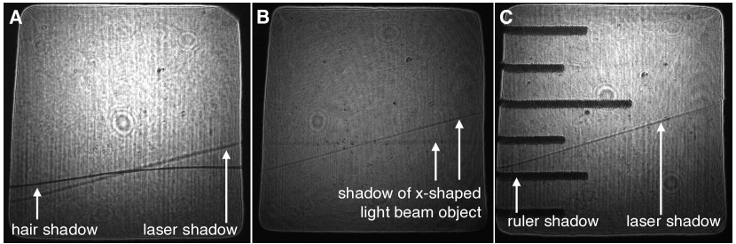
Figure 4: Qualitative comparison of the laser shadow to normal shadows. Three direct images of the transmitted illuminating light containing multiple simultaneous shadows. (A) A human hair produces a very similar shadow to that of the object laser beam ($P=20$ W). (B) The shadow of an object made of two crossed laser beams, showing that the laser shadow has the same shape as the object (total $P=20$ W). (C) For scale, a shadow of the object laser beam ($P=15$ W) with a ruler (imperial, small increments are $1/6"=1.588$ mm).

A simplified schematic of the experimental setup is presented in Fig 2 (C) and a detailed schematic is given in the Supplementary Material along with a comprehensive description. We outline the key elements of the experiment here. A continuous wave (CW) laser diode creates the blue illuminating light which is collimated and enlarged with lenses to fill the the ruby cube, which has an edge length of $12.0\pm 0.5$ mm and a doping of $2.5\crossproduct 10^{25}$ m${}^{-3}\pm 10\%$. The green object laser is produced by a CW diode-pumped solid-state laser. The theoretical model shows that the local opacity of the green laser beam saturates at high intensities, i.e., any chosen point in the laser beam object will be translucent to the blue illumination. By increasing the object beam thickness along $x$, the direction along the illumination, we maximize the interaction length between the object and the illumination lights. To accomplish this, the object beam has an elliptical profile, i.e., approximately Gaussian, with $1/e^{2}$ intensity half-widths of $w_{0x}=3.17\pm 0.01$ mm and $w_{0y}=0.168\pm 0.003$ mm in the $x$ and $y$ directions, respectively. Absorption of the green laser heats the cube, which changes the phonon population and lattice spacing and, in turn, the opacity. Consequently, we limit the heating time as needed to keep the cube’s temperature low, which we monitor. Images were taken in two different ways. The first was designed to capture what is seen by eye. In it, a mirror reflects the transmitted blue illumination towards a piece of paper, which is then photographed using a digital consumer camera and a lens (see Fig. 1, discussed in the Introduction and the Supplementary Material). In the second way, a scientific monochrome camera is directly in the path of the transmitted blue light in order to take quantitative data, which we present next.

We now describe how we quantitatively analyze these images and compare them to our theoretical model. Figure 3 (A) shows a typical image obtained by the scientific camera when the object laser power is set to $P=15$ W, clearly showing the laser shadow. We take a set of 21 images used for normalization without the object (green) laser, followed by 21 images with the object (green) laser, and thus, shadow present. For all the images we integrate along $z$, resulting in a distribution in $y$ only. We divide each shadow-image distribution $s(y)$ by the normalization-image distribution $n(y)$ to find the relative transmittance at each $y$ position, $T(y)\equiv s(y)/n(y)$. The mean relative transmittance and its standard error over 21 images is shown in Fig. 3 (B). In the absence of a shadow, nominally $T(y)=1$ at all $y$, whereas a perfectly black shadow would have $T=0$. Continuing this procedure, we take 21 images for each of six object laser powers spanning from $P=$ 5 W to 17 W (measured just before the cube). Fig. 3 (B) shows the resulting experimental relative transmittance along with the corresponding theoretical curves with error bands found from the uncertainties in the parameters in the model (see Supplementary Material) . To facilitate comparing between different configurations of object laser (green) optical power and for sake of clarity of the figure, each set of graphs for a given power is vertically shifted by 0.2 with a solid black line to indicate a reference level for the drop in transmittance according to that level.

The experimental relative transmittance reveals a few important characteristics of the laser shadow effect. The experiment and theoretical model agree well for the largest drop in transmittance, suggesting that our physical model correctly predicts the maximum amount of illumination that is blocked. However, the width of the theoretical shadow is approximately twice that of the measured shadow. An unexpectedly narrow shadow could potentially point to other non-shadow-like nonlinear optical effects playing a role in the formation of the observed dark region. For example, nonlinear optical refraction by the object beam could divert the illumination rather than block it, creating dark regions much like those formed at the bottom of a swimming pool by surface waves. To distinguish between these possible causes, we compare the shadow shape to the profile along $y$ of the object laser beam. A Gaussian fit (Fig. 3 (B), solid red line) to the object beam’s profile closely follows the experimental profile, albeit not within error. This confirms the expectation that the shadow should be the same as size as the object (criteria (iv)) and that it is caused by blocking rather than diverting the illuminating light (criteria (iii)). Another possible hypothesis for the width discrepancy between measurements and the theoretical model is a self-focusing process as the object laser beam (green) goes through the ruby cube hogan2023 .

The darkness of a shadow is its main characteristic and so we now investigate this more thoroughly. More specifically, we compare the darkness to the illumination using the contrast $\mathcal{C}$:

$$\mathcal{C}\equiv\frac{T^{top}(y_{\mathrm{min}})-T^{bottom}\left(y_{\mathrm{min}}\right)}{T^{top}(y_{\mathrm{min}})},$$ (1)

where, over all $y$, $T^{bottom}(y_{\mathrm{min}})$ is the minimum value of transmittance $T$ for the illumination laser beam (blue), i.e., darkest transmitted value, with the object laser beam (green) present, while $T^{top}(y_{\mathrm{min}})$ is the value of transmittance $T$ for the illumination laser beam (blue) at the same position, $y_{\mathrm{min}}$, when the object laser beam (green) is absent. Essentially, the contrast $\mathcal{C}$ is a normalized metric of the drop in transmittance of the illumination laser beam (blue).

The graph of the experimental contrast as a function of optical power of the green laser is reported in Fig. 3 (C), together with a linear fit ($\mathcal{C}=mP,m=1.38\pm 0.03\leavevmode\nobreak\ \%/\mathrm{W}$) and the theoretical predictions for each of the six powers. To evaluate the quality of the linear fit, we obtained $R^{2}=0.9669$ and $\chi^{2}=0.307$, which means that the linear distribution is a good fit of the observed data hogg1977probability . The linearity shows that the object beam is far from saturating the ${}^{4}\text{A}_{2}$ to ${}^{4}\text{T}_{2}$ transition, as was the goal of creating the elliptical object beam. The maximum contrast achieved was $22.1\pm 0.6$% with $17.04\pm 0.02$ W in the object beam. For this case, we infer an attenuation coefficient that the illuminating light experiences while it travels through the object beam, $\alpha=173.6\leavevmode\nobreak\ \mathrm{m^{-1}}$ (the $\alpha$ in Eq. 8 in the Supplementary Material). We conclude that as the object laser beam power increases, the deeper the drop in transmittance of the illuminating blue light, leading to a greater magnitude of the laser shadow effect, which in turn is manifested as a greater contrast value.

In this last part, we return to our qualitative observations, namely comparisons of the laser shadow to a regular shadow made from a material object. Fig. 4 presents three direct images, taken with the scientific camera, each showing a different comparison. In Fig. 4 (A), while the object beam is present, we place a strand of black hair in the path of illuminating blue light before the cube. Unsurprisingly, the black hair is more opaque than the object laser beam, which transmits almost 80% of the illumination, and casts a darker shadow. Nonetheless, without the labels, it would be difficult to decide which shadow is which. In Fig. 4 (B), we split and divert the green laser using a beam displacer and prism with the goal of changing the light object to be x-shaped, i.e., two beams crossing at an acute angle. As with the shadow of a material object, the laser shadow in the image takes on the new shape of the object (e.g., as with shadow puppets) confirming criteria (iv), i.e., the laser shadow is x-shaped. In Fig. 4 (C), a ruler, placed before the ruby cube, and the object laser are both present, showing the length-scale of the effect (criteria (i)), and thus its macroscopic manifestation. To confirm the final criteria, in the Supplemental Material, we include a real-time video of one of the object laser beam changing in angle and position. Just as criteria (v) demanded, the shadow follows the object beam as it moves without an observable delay by the human eye.

The laser shadow effect requires a ruby to mediate this blockage, which raises the interesting question of whether the photons in the object laser themselves are blocking the illuminating light or rather it is the atoms in the ruby. A analogous question — is a light wave propagating in a material made up of photons or excitations in atoms? — applies to established effects such as slowed or stopped light and, indeed, even everyday transmission through a glass window. While, fundamentally, the wave is actually composed of a hybrid of the two, “polaritons”, for most purposes it suffices to consider the light in the material to be made of photons. We apply this common interpretation to the light shadow effect: object beam photons are blocking illumination photons.

III Conclusion

We showed how a laser beam can be made to cast a shadow that behaves as any other ordinary shadow. To that point, the laser shadow obeys six straightforward criteria that distinguish ordinary shadows from other phenomena that are superficially similar, such as nonlinear optical refraction, light-darkening glass, temperature-sensitive mirrors, or laser-induced damage in glass. Of particular importance is that we found a successful agreement of our analytical physical model with our quantitative observations, showing that the mechanism behind the laser shadow is a blockage of the illuminating light.

Other materials such as alexandrite are expected to also be able to show the laser shadow effect malcuit1984saturation_alexandrite .

This experiment redefines our understanding of what a shadow is – something massless can cast a shadow. Potential applications can be envisioned in areas such as optical switching dawes2005all , controllable shade or transmission, control of the opaqueness of light with light, and lithography.

Authors Contributions: The project was conceived by JSL, AS and RWB. The experiment was built by RAA, JTRP and HPNM. Data was taken and analysed by RAA, HPNM and JTRP. Manuscript was written by RAA, HPNM and JSL, with inputs from all authors. The theoretical simulation was initially developed by AS, and further improved and used by HPNM and RAA. JSL supervised the project.

IV ACKNOWLEDGMENTS

This work was supported by the Canada Research Chairs (CRC) Program, the Natural Sciences and Engineering Research Council (NSERC), the Canada Excellence Research Chairs (CERC) Program, the Canada First Research Excellence Fund award on Transformative Quantum Technologies, the U.S. Department of Energy QuantISED award, and the Brookhaven National Laboratory LDRD grant 22-22. HPNM acknowledges support from the Canada Graduate Scholarships - Master’s (CGS-M) program.

SUPPLEMENTARY MATERIAL

Methods

The analysis begins with the images taken from the scientific CMOS camera, taken at the maximum resolution of 3088 x 2076 pixels. The images are cropped to the ruby, keeping the resolution but reducing the size of the image to only the relevant part of the image. Several datasets are collected. A background set was collected with only the illuminating blue laser, to be used as the reference for all other powers. Datasets were taken with the green object laser at several power values. Each dataset comprises of $21$ total images. This is obtained from the movement of the translation stage during data collection (total 2 mm displacement in steps of 0.1 mm in the $y$ dimension). Each individual dataset is averaged into a single image. We integrate over the $z$ dimension in each image. The result of this integration is Eq. 8. The position of the local minimum in the graph of the transmittance of the blue laser is determined. The maximum value obtained at this position is obtained through the background result. Combined, these two values are used to compute the contrast for that power of the green object laser.

The calculation of the contrast is discussed in the next paragraph. Since the normalization used is based on an experimental parameter, i.e., the background image when the green laser was off, it can happen that for some values the error bars cross the value of 1.0 of transmittance for a given reference value. However transmittance above 1.0 is meaningless. This issue is more relevant for low powers of the green laser.

Theoretical Simulations

Deriving the Model

The laser shadow effect is modeled through the use of rate equations for the populations of the $\ce{Cr^{3}+}$ ions in ruby. Let $N$ be the total number density of ions in the ruby, $N_{1}$ the number density in the $\ket{1}=\ket{{}^{4}\text{A}_{2}}$ state, and $N_{3}$ the number density in the $\ket{3}=\ket{{}^{2}\text{E}}$ state. The lifetimes of the $\ket{2}=\ket{{}^{4}\text{T}_{2}}$ and $\ket{4}=\ket{{}^{2}\text{T}_{1}}$ are negligible and can be neglected. The total population is therefore:

$$N=N_{1}+N_{3}.$$ (2)

Hence, the population in the $N_{1}$ state is given by:

$$\derivative{N_{1}}{t}=-\dfrac{I}{\hbar\omega}\sigma_{1}N_{1}+\dfrac{N_{3}}{T_{3}},$$ (3)

where $\sigma_{1}$ is the absorption cross-section of the first transition for the $532$ nm object laser, $T_{3}$ is the lifetime of the metastable $\ket{3}$ state, $I$ is the intensity of the $532$ nm object laser, $\hbar$ is the reduced Planck constant, and $\omega$ is the angular frequency of the $532$ nm object laser. We define the saturation intensity as:

$$I_{S}=\dfrac{\hbar\omega}{T_{3}\sigma_{1}}.$$ (4)

We solve Eq. 3 at steady state ($\derivative{N_{1}}{t}=0$) condition. Eliminating $N_{3}$ from the solution gives us:

$$N_{1}=\dfrac{N}{1+1/I_{S}}.$$ (5)

From the definition of the absorption cross-section, we can write:

$$\alpha^{\text{blue}}(I)=\sigma_{1}^{\text{blue}}N_{1}+\sigma_{3}^{\text{blue}}N_{3}.$$ (6)

Using Equations 2 and 5, Equation 6 is simplified to only contain the total number density $N$. We then obtain an expression for the absorption of the illuminating blue laser as a function of the intensity of the green object laser:

$$\alpha^{\text{blue}}\left(I\right)=\frac{\sigma_{1}^{\text{blue}}N}{1+I\frac{\sigma_{1}^{\text{green}}T_{3}}{\hbar\omega}}+\sigma_{3}^{\text{blue }}N\left(1-\frac{1}{1+I\frac{\sigma_{1}^{\text{green}}T_{3}}{\hbar\omega}}\right)$$ (7)

This expression is then integrated over the $z$ dimension to obtain:

$$I(y)=I_{0}e^{-\int_{0}^{L}\alpha^{\text{blue}}(y,z)\differential{z}}.$$ (8)

where $L$ is the length of the ruby crystal and $I_{0}$ is the background intensity. This equation is our model of the effect.

Using the Model

Several parameters need to be experimentally obtained to evaluate Eq. 8. These include: the beam waists $w_{0x}$ and $w_{0y}$ of the green laser (acting as the illuminated object), $N$ the number density of the $\ce{Cr^{3}+}$ ions in the ruby, $\sigma_{1}^{\text{blue}}$ and $\sigma_{1}^{\text{green}}$, the absorption cross-sections of both laser beams for the first transition, and $\sigma_{3}^{\text{blue}}$ the absorption cross-section of the illuminating blue laser for the second transition. The lifetime $T_{3}$ will be used as a fit parameter.

The beam waists were experimentally determined using the razor blade method. For these measurements, the blade was $\sim 10$ mm away from the ruby in the $x$ dimension and $\sim 20$ mm in the $y$ dimension. The uncertainties attributed are the errors on the fit. We measured: $w_{0x}=3.17\pm 0.01$ mm and $w_{0y}=0.168\pm 0.003$ mm.

To obtain values for the absorption cross-sections for the first transition, we use Beer’s Law:

$$T_{j}=e^{-\sigma_{1}^{j}NL},$$ (9)

where $T_{j}$ is the transmission of the $j$th wavelength through the ruby, $\sigma_{1}^{j}$ is the absorption cross-section for the first transition for the $j$th wavelength, $N$ is the total number density of $\ce{Cr^{3}+}$ ions in the ruby, and $L$ is the length of the ruby. The length was measured at $L=12.0\pm 0.5$ mm in both the $z$ and $x$ dimensions. To evaluate Eq. 9, we need to measure $T_{j}$.

Transmission values were obtained in the linear regime for both wavelengths. For the $450$ nm illumination laser, the average power at the ruby was $285\,\mu$W. To measure the transmission of the green laser ($532$ nm, object laser), we set the green laser to a low power such that the average power reaching the cube was measured to be $934\,\mu$W. For both cases, transmission data was obtained by measuring the power before and after the ruby over $10$ minutes, in the respective propagation path. The $450$ nm illumination laser was allowed to stabilize for $5$ hours before taking measurements. This raw data is then Fresnel corrected, using $n_{\text{ruby}}=1.77$ and $n_{\text{air}}=1.0003$. Errors are obtained by taking the standard deviation of the measurements. We obtain $T_{\text{blue}}=26.01\pm 0.02\%$ and $T_{\text{green}}=26.8\pm 0.3\%$. Thus these values are used to solve Eq. 9 simultaneously for $\sigma_{1}$ for both wavelengths.

Fitting the model against the experimental data allowed us to set the remaining three (3) unknowns, which are the total number density $N$, the absorption cross-section for the second transition for the $450$ nm illumination laser $\sigma_{3}^{\text{blue}}$, and the lifetime $T_{3}$. We obtained $N=2.5\times 10^{25}\text{ m}^{-3}$ and $\sigma_{3}^{\text{blue}}=17.2\times 10^{-24}\text{ m}^{2}$. The uncertainty on both of these values was set at $\pm 10\%$ as reported in Ref. cronemeyer1966optical . The initial value of the metastable state’s lifetime $T_{3}$ was initially set at $T_{3}=3$ ms, per the literature huang1968 . However, due to the temperature increase of the ruby, this value proved to be inaccurate and was reduced to $T_{3}=1$ ms.

Obtaining the Uncertainty Bands

The theoretical error bands as presented in fig. 3 of the main text are determined as follows. The center theory curve is calculated using the mean values of all respective parameters. The model is then computed taking the extreme values of each parameter, individually. This allows us to isolate the effect of changing only a single parameter on the model. We take note at which parameters increase and which decrease the minimum value of the curve. The errors are then normalized in the same manner as previously indicated. All parameters which increase (decrease) the value of the minimum are added in quadrature. These values are then added (subtracted) from the central theory curve to obtain the error bands.

Experimental Setup in Detail

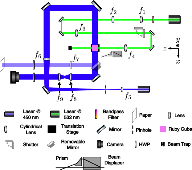
Figure 5: Complete Experimental Setup. The setup of Fig. 2 (C) is expanded upon to include additional elements.

All images in Figure 1 were taken using an Olympus OM-D EM-5 Mark II with a M. Zuiko 17mm f/1.8 prime lens. Figure 5 gives further information about the experimental setup. The illumination laser is a 450 nm 4.5 mW diode blue laser. The optical power which covered the face of the ruby is 285.06 $\mu$W. The object laser is a Millennia eV 532 nm CW laser, whose optical power output is adjustable and is in the $\text{TEM}_{\text{00}}$ spatial mode. This laser is shaped into an ellipse stretched in the $x$ dimension using two pairs of cylindrical lenses. The first pair ($f_{1}=100$ mm, $f_{2}=400$ mm) stretches the beam in the $x$ dimension and the second pair ($f_{3}=500$ mm, $f_{4}=50$ mm) squeezes in $y$. The other lenses in the setup are: $f_{5}=45$ mm, $f_{6}=1000$ mm, $f_{7}=125$ mm, $f_{8}=300$ mm, and $f_{9}=50$ mm. The bandpass filter used was a 450 $\pm$ 8 nm CWL, 40 $\pm$ 8 nm FWHM filter. The same filter is used in the CMOS images, as well as in the photography camera images, just moved from one optical path to the other.

Temperature Dependence

Variations in temperature change the optical properties of ruby, as previously studied in Ref. Kiang1965 . In our experiment, the presence of the green object laser can significantly increase the temperature of the ruby crystal. This causes a reduction in the observed contrast of the laser shadow, as seen in Fig. 6. Furthermore, this also causes the contrast to have a nonlinear relationship as a function of input power, which goes against our model. For these reasons, we used a shutter in the green laser’s path to limit the amount of time the ruby will be exposed to intense light, reducing the overall temperature effects. The shutter was set such that it exposes the ruby to the green object laser for $\approx$ 500 ms. Once a full dataset was obtained, the ruby is allowed to cool down to room temperature ($23$ °C) before the next dataset is collected. All data presented in our quantitative analysis as reported in Fig. 3 (B) and (C) were taken using this control mechanism.

For the nonlinear behavior of Fig. 6, our hypothesis is that the heating of the ruby cube affects the populations of the atomic levels, so that the effect as described in section Theory is impaired, leading to a reduction in the contrast. Table 1 reports the measured temperatures both with and without the shutter, demonstrating the large temperature difference observed.

Attenuation Coefficient

We report in Table 2 the attenuation coefficient $\alpha$, mathematically defined in Eq. 8, as the illuminating laser beam travels through the object laser beam for different optical powers of the object laser beam.

Laser Shadow Video

We included as Supplementary Material a 50s real-time video (mp4 format) in which one can see the laser shadow moving as the prism in the object laser beam (green) path was being manually tilted. This video was recorded with object laser beam (green) set to 20 W of optical power.

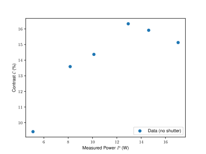
Figure 6: Shadow contrast affected by temperature. This graph shows the measured shadow contrasts for varying green laser optical power in the ruby cube when data was taken without the shutter (i.e., without temperature control).

Nominal Power (W)	Temperature (°C)	Temperature (°C)
	Without Shutter	With Shutter
5	63	26
8	82	28
10	96	29
13	112	31
15	124	32
18	137	34

Table 1: Power vs. Temperature. Measurements of the temperature of ruby cube with and without the temperature control for different nominal power values of the object laser beam (green).

Nominal Power (W)	Attenuation coefficient $\alpha$ $(\mathrm{m^{-1}})$
5	133.5
8	144.9
10	151.8
13	161.1
15	166.3
18	173.6

Table 2: Attenuation coefficient. Attenuation coefficient as the illuminating laser beam (blue) travels through the object laser beam (green) for different nominal power values of the object laser beam (green).

References

- (1) C. K. Hong, Z. Y. Ou, and L. Mandel, “Measurement of subpicosecond time intervals between two photons by interference,” Phys. Rev. Lett., vol. 59, pp. 2044–2046, Nov 1987.
- (2) F. Bouchard, A. Sit, Y. Zhang, R. Fickler, F. M. Miatto, Y. Yao, F. Sciarrino, and E. Karimi, “Two-photon interference: the Hong–Ou–Mandel effect,” Reports on Progress in Physics, vol. 84, no. 1, p. 012402, 2020.
- (3) K. M. Jordan, R. A. Abrahao, and J. S. Lundeen, “Quantum metrology timing limits of the Hong-Ou-Mandel interferometer and of general two-photon measurements,” Phys. Rev. A, vol. 106, p. 063715, Dec 2022.
- (4) R. W. Boyd, Nonlinear Optics. Academic Press, 2020.
- (5) A. V. Gorshkov, J. Otterbach, M. Fleischhauer, T. Pohl, and M. D. Lukin, “Photon-photon interactions via Rydberg blockade,” Phys. Rev. Lett., vol. 107, p. 133602, Sep 2011.
- (6) H. Busche, P. Huillery, S. W. Ball, T. Ilieva, M. P. Jones, and C. S. Adams, “Contactless nonlinear optics mediated by long-range Rydberg interactions,” Nature Physics, vol. 13, no. 7, pp. 655–658, 2017.
- (7) O. Firstenberg, T. Peyronel, Q.-Y. Liang, A. V. Gorshkov, M. D. Lukin, and V. Vuletić, “Attractive photons in a quantum nonlinear medium,” Nature, vol. 502, no. 7469, pp. 71–75, 2013.
- (8) G. A. Mourou, T. Tajima, and S. V. Bulanov, “Optics in the relativistic regime,” Rev. Mod. Phys., vol. 78, pp. 309–371, Apr 2006.
- (9) M. Marklund, “Probing the quantum vacuum,” Nature Photonics, vol. 4, no. 2, pp. 72–74, 2010.
- (10) D. Bernard, F. Moulin, F. Amiranoff, A. Braun, J. Chambaret, G. Darpentigny, G. Grillon, S. Ranc, and F. Perrone, “Search for stimulated photon-photon scattering in vacuum,” The European Physical Journal D-Atomic, Molecular, Optical and Plasma Physics, vol. 10, no. 1, pp. 141–145, 2000.
- (11) B. King and T. Heinzl, “Measuring vacuum polarization with high-power lasers,” High Power Laser Science and Engineering, vol. 4, p. e5, 2016.
- (12) A. J. Macleod, J. P. Edwards, T. Heinzl, B. King, and S. V. Bulanov, “Strong-field vacuum polarisation with high energy lasers,” New Journal of Physics, vol. 25, p. 093002, sep 2023.
- (13) A. Safari, C. Selvarajah, J. Evans, J. Upham, and R. W. Boyd, “Strong reverse saturation and fast-light in ruby,” arXiv:2301.13300, 2023.
- (14) R. W. Boyd, A. L. Gaeta, and E. Giese, “Nonlinear optics,” in Springer Handbook of Atomic, Molecular, and Optical Physics, pp. 1097–1110, Springer, 2008.
- (15) M. S. Bigelow, N. N. Lepeshkin, and R. W. Boyd, “Superluminal and slow light propagation in a room-temperature solid,” Science, vol. 301, no. 5630, pp. 200–202, 2003.
- (16) G. M. Gehring, A. Schweinsberg, C. Barsi, N. Kostinski, and R. W. Boyd, “Observation of backward pulse propagation through a medium with a negative group velocity,” Science, vol. 312, no. 5775, pp. 895–897, 2006.
- (17) M. A. Kramer, W. R. Tompkin, and R. W. Boyd, “Nonlinear-optical interactions in fluorescein-doped boric acid glass,” Physical Review A, vol. 34, no. 3, p. 2026, 1986.
- (18) M. S. Bigelow, N. N. Lepeshkin, and R. W. Boyd, “Observation of ultraslow light propagation in a ruby crystal at room temperature,” Physical Review Letters, vol. 90, no. 11, p. 113903, 2003.
- (19) S. Franke-Arnold, G. Gibson, R. W. Boyd, and M. J. Padgett, “Rotary photon drag enhanced by a slow-light medium,” Science, vol. 333, no. 6038, pp. 65–67, 2011.
- (20) D. Cronemeyer, “Optical absorption characteristics of pink ruby,” JOSA, vol. 56, no. 12, pp. 1703–1705, 1966.
- (21) T. H. Maiman, “Optical and microwave-optical experiments in ruby,” Phys. Rev. Lett., vol. 4, pp. 564–566, Jun 1960.
- (22) T. Maiman, “Stimulated optical radiation in ruby,” Nature, vol. 187, no. 4736, pp. 493–494, 1960.
- (23) R. Boyd and D. Gauthier, Progress in Optics 43. Chapter 6. Elsevier, Amsterdam, 2002.
- (24) R. W. Boyd and D. J. Gauthier, “Controlling the velocity of light pulses,” Science, vol. 326, no. 5956, pp. 1074–1077, 2009.
- (25) Y. Kiang, J. Stephany, and F. Unterleitner, “Visible spectrum absorption cross section of Cr3+ in the 2E state of pink ruby,” IEEE Journal of Quantum Electronics, vol. 1, no. 7, pp. 295–298, 1965.
- (26) In Fig. 3 (B), it is possible that some experimental values of the normalized Transmittance could display values above 1.0. This is purely an artifact of the mathematical normalization based on a real image, no physical meaning is associated to that.
- (27) R. Hogan, A. Safari, G. Marcucci, B. Braverman, and R. W. Boyd, “Beam deflection and negative drag in a moving nonlinear medium,” Optica, vol. 10, no. 5, pp. 544–551, 2023.
- (28) R. V. Hogg, E. A. Tanis, and D. L. Zimmerman, Probability and statistical inference, vol. 993. Macmillan New York, 1977.
- (29) M. S. Malcuit, R. W. Boyd, L. W. Hillman, J. Krasinski, and C. Stroud, “Saturation and inverse-saturation absorption line shapes in alexandrite,” JOSA B, vol. 1, no. 1, pp. 73–75, 1984.
- (30) A. M. Dawes, L. Illing, S. M. Clark, and D. J. Gauthier, “All-optical switching in rubidium vapor,” Science, vol. 308, no. 5722, pp. 672–674, 2005.
- (31) J. W. Huang and H. W. Moos, “Absorption Spectrum of Optically Pumped :,” Phys. Rev., vol. 173, pp. 440–444, Sep 1968.