McCatch: Scalable Microcluster Detection in Dimensional and Nondimensional Datasets

Abstract

How could we have an outlier detector that works even with nondimensional data, and ranks together both singleton microclusters (‘one-off’ outliers) and nonsingleton microclusters by their anomaly scores? How to obtain scores that are principled in one scalable and ‘hands-off’ manner? Microclusters of outliers indicate coalition or repetition in fraud activities, etc.; their identification is thus highly desirable. This paper presents McCatch: a new algorithm that detects microclusters by leveraging our proposed ‘Oracle’ plot ($1$NN Distance versus Group $1$NN Distance). We study $31$ real and synthetic datasets with up to $1$M data elements to show that McCatch is the only method that answers both of the questions above; and, it outperforms $11$ other methods, especially when the data has nonsingleton microclusters or is nondimensional. We also showcase McCatch’s ability to detect meaningful microclusters in graphs, fingerprints, logs of network connections, text data, and satellite imagery. For example, it found a $30$-elements microcluster of confirmed ‘Denial of Service’ attacks in the network logs, taking only $\mathit{\sim 3}$ minutes for $222$K data elements on a stock desktop.

I Introduction

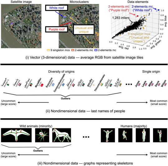
Figure 1: McCatch is unsupervised, and it ALSO works on nondimensional data: (i) on vector, $3$d data from a satellite image of Shanghai – it spots two $2$-elements microclusters of unusually colored roofs, and a few other outliers; on nondimensional data of last names (ii) and skeletons (iii) – it gives high anomaly scores to the few nonenglish names and skeletons of wild animals. (best viewed in color)

How could we have a method that detects microclusters of outliers even in a nondimensional dataset? How to rank together both singleton (‘one-off’ outliers) and nonsingleton microclusters according to their anomaly scores? Can we define the scores in a principled way? Also, how to do that in a scalable and ‘hands-off’ manner? Outlier detection has many applications and extensive literature [1, 2, 3]. The discovery of microclusters of outliers is among its most challenging tasks. It happens because these outliers have close neighbors that make most algorithms fail [4, 5, 6]. For example, see the red elements in the plots of Fig. 1(i) and Fig. 2. Microclusters are critical for settings such as fraud detection and prevention of coordinated terrorist attacks, to name a few, because they indicate coalition or repetition as compared to ‘one-off’ outliers. For example, a microcluster (or simply ‘mc’, for short) can be formed from: (i) frauds exploiting the same vulnerability in cybersecurity; (ii) reviews made by bots to illegitimately defame a product in e-commerce, or; (iii) unusual purchases of a hazardous chemical product made by ill-intended people. Its discovery and comprehension is, therefore, highly desirable.

We present a new microcluster detector named McCatch – from Microcluster Catch. The main idea is to leverage our proposed ‘Oracle’ plot, which is a plot of $1$NN Distance versus Group $1$NN Distance with the latter being the distance from a cluster of data elements to its nearest neighbor. Our goals are:

1. General Input: to work with any metric dataset, including nondimensional ones, such as sets of graphs, short texts, fingerprints, sequences of DNA, documents, etc.

2. General Output: to rank singleton (‘one-off’ outliers) and nonsingleton mcs together, by their anomalousness.

3. Principled: to obey axioms.

4. Scalable: to be subquadratic on the number of elements.

5. ‘Hands-Off’: to be automatic with no manual tuning.

We studied $31$ datasets with up to $1$M elements to show that McCatch achieves all five goals, while $11$ of the closest state-of-the-art competitors fail. Fig. 1 showcases McCatch’s ability to process dimensional and nondimensional data: (i) On vector, $3$d data from a satellite image of Shanghai, it spots two $2$-elements mcs of buildings with unusually colored roofs, and; a few other outliers. On nondimensional data of last names  (ii) and skeletons (iii), it gives high anomaly scores to the few nonenglish names and wild-animal skeletons. The details of this experiment are given later; see Sec. V.

II Problem & Related Work

II-A Problem Statement

Problem 1 (Main problem)

It is as follows:

• Given:

  • a metric dataset $\mathbf{P}~{}=~{}\{\mathbf{p}_{1},\dots\mathbf{p}_{n}\}$, where $\mathbf{p}_{i}$ is a data element (‘point’, in a dimensional case);

  • a distance/dis-similarity function $\mathtt{f}(\mathbf{p}_{i},\mathbf{p}_{i^{\prime}})$ (e.g., Euclidean / $L_{p}$ for dimensional data; provided by domain expert for non-dimensional data).

• Find: (i) a set of disjoint microclusters $\mathcal{M}=\{\mathbf{M}_{1},\dots$ $\mathbf{M}_{m}\}$, ranked most-strange-first, and (ii) the set of corresponding anomaly scores $\mathcal{S}=\{s_{1},\dots s_{m}\}$

• to match human intuition (see the axioms in Fig. 2).

For ease of explanation, from now on, we shall describe our algorithm using the term ‘point’ for each data element. However, notice that the algorithm only needs a distance function between two elements – NOT coordinates.

II-B Related Work

There is a huge literature on outlier and microcluster detection. However, as we show in Tab. I, only our McCatch meets all the specifications. Next, we go into more detail.

Related work vs. goals

Outlier detection has many applications, including finance [7, 8], manufacturing [9, 10], environmental monitoring [11, 12], to name a few. It is thus covered by extensive literature [1, 2, 3]. The existing methods can be categorized in various ways, for example, based on the measures they employ, including density-, depth-, angle- and distance-based methods, or by their modeling strategy, such as statistical-modeling, clustering, ensemble, etc., among others.

TABLE I: McCatch matches all specs, while the competitors miss one or more of the features.

Classic

Deep

Clustering

ABOD [13]

ALOCI [14]

DB-Out [15]

DIAD [16]

D.MCA [5]

FastABOD [13]

Gen2Out [4]

GLOSH [17]

iForest [18]

kNN-Out [19]

LDOF [20]

LOCI [14]

LOF [21]

ODIN [22]

PLDOF [23]

SCiForest [6]

Sparkx [24]

XTreK [25]

Deep SVDD [26]

DOIForest [27]

RDA [28]

DBSCAN [29]

KMeans– [30]

OPTICS [31]

McCatch

G1. General Input

?

?

?

?

?

?

?

?

?

?

✔

G2. General Output

✓

✔

G3. Principled (group axioms)

✔

G4. Scalable

✓

✓

✓

✓

✓

✓

✓

✓

✓

✓

✓

✔

G5. ‘Hands-Off’

✓

✓

✓

✓

✓

✓

✓

✓

✓

✔

Deterministic

✓

✓

✓

✓

✓

✓

✓

✓

✓

✓

✓

✔

Explainable Results

✓

✓

✓

✓

✓

✓

✓

✓

✓

✓

✓

✓

✓

✓

✓

✓

✓

✓

✓

✓

✓

✔

Rank Results

✓

✓

✓

✓

✓

✓

✓

✓

✓

✓

✓

✓

✓

✓

✓

✓

✓

✓

✓

✓

✓

✔

This section presents the related work in a nontraditional way. We describe it considering the goals of our introductory section as we understand an ideal method should work with a General Input (G1) and give a General Output (G2) that is Principled (G3) in a Scalable (G4) and ‘Hands-Off’ (G5) way.

General Input– goal G1

Many methods fail w.r.t. G1. It includes famous isolation-based detectors, e.g., iForest [18], Gen2Out [4], and SCiForest [6], other tree-based methods, such as XTreK [25] and DIAD [16], hash-based approaches, e.g., Sparkx [24], angle-based ones, like ABOD/FastABOD [13], some clustering-based methods, e.g., KMeans– [30] and PLDOF [23], and even acclaimed deep-learning-based detectors, such as RDA [28], DOIForest [27], and Deep SVDD [26]. They all require access to explicit feature values. Note that embedding may allow these methods to work on nondimensional data. Turning elements of a metric or non-metric space into low-dimensionality vectors that preserve the given distances is exactly the problem of multi-dimensional scaling [32] and more recently t-SNE and UMAP [33]. However, these strategies have two disadvantages: (i) they are quadratic on the count of elements [34], and; (ii) they require as input the embedding dimensionality. Distinctly, density- and distance-based detectors – as well as some clustering methods that detect outliers as a byproduct of the process, like DBSCAN [29] and OPTICS [31] – may handle nondimensional data if adapted to work with a suitable distance function, and, ideally, also with a metric tree, like a Slim-tree [35] or an M-tree [36]. Examples are LOCI [14], LOF [21], GLOSH [17], kNN-Out [19], DB-Out [15], ODIN [22], LDOF [20], and D.MCA [5]. However, faster hypercube-based versions of some of these methods, e.g., ALOCI [14], require the features.

General Output– goal G2

Most methods fail in G2. They miss every mc whose points have close neighbors, like ABOD, iForest, LOCI, Deep SVDD, RDA, GLOSH, kNN-Out, LOF, DB-Out, ODIN, DIAD, Sparkx, XTreK, and DOIForest; or, fail to group these points into an entity with a score, e.g., D.MCA, SCiForest, LDOF, PLDOF, DBSCAN, OPTICS, and KMeans–. Gen2Out is the only exception.

Principled– goal G3

Goal G3 regards the generation of scores in a principled manner for both singleton and nonsingleton mcs. Gen2Out is the only method that provides scores for microclusters; thus, all other methods fail to achieve G3. Unfortunately, Gen2Out also fails w.r.t. G3 as it does not identify nor obey any axiom for generating microcluster scores. It does not obey axioms that we propose either.

Scalable– goal G4

Some methods are scalable, like ALOCI, iForest, Gen2Out, SCiForest, PLDOF, KMeans–, Sparkx, XTreK, DOIForest, RDA, and Deep SVDD. They achieve G4. Distinctly, methods like DIAD, D.MCA, ABOD, FastABOD, GLOSH, LOCI, kNN-Out, LOF, DB-Out, ODIN, LDOF, DBSCAN, and OPTICS fail in G4 as they are quadratic (or worse) on the count of points.

‘Hands-Off’– goal G5

Goal G5 regards the ability of a method to process an unlabeled dataset without manual tuning. Methods that achieve G5 are either hyperparameter free, like ABOD; or, they have a default hyperparameter configuration to be used in all datasets, as it happens with FastABOD, Gen2Out, D.MCA, iForest, SCiForest, GLOSH, LOCI, and XTreK. On the other hand, many methods fail w.r.t. G5. Examples are ALOCI, DB-Out, kNN-Out, LOF, LDOF, PLDOF, DBSCAN, OPTICS, KMeans–, RDA, Deep SVDD, ODIN, DIAD, Sparkx, and DOIForest as they all require user-defined hyperparameter values.

Conclusion: Only McCatch meets all the specifications

As mentioned earlier, and as shown in Tab. I, only McCatch fulfills all the specs. Additionally, in contrast to several competitors, our method is deterministic and ranks outliers by their anomalousness. McCatch also returns explainable results thanks to the plateaus of our ‘Oracle’ plot (See Sec. IV-A), which roughly correspond to the distance to the nearest neighbor. Distinctly, black-box methods suffer on explainability.

III Proposed Axioms

How could we verify if a method reports scores in a principled way? To this end, we propose reasonable axioms that match human intuition and, thus, should be obeyed by any method when ranking microclusters w.r.t. their anomalousness. Importantly, our axioms apply to singleton and also to nonsingleton microclusters, so that both ‘one-off’ outliers and ‘clustered’ outliers are included seamlessly into a single ranking.

The axioms state that the score $s_{j}$ of a microcluster $\mathbf{M}_{j}$ depends on: (i) the smallest distance between any point $\mathbf{p}_{i}\in\mathbf{M}_{j}$ and this point’s nearest inlier – let this distance be known as the ‘Bridge’s Length’ $\overset{\downarrow}{g}\overset{{\left(j\right)}}{}$ of $\mathbf{M}_{j}$, and; (ii) the cardinality $\mid\mathbf{M}_{j}\mid$ of $\mathbf{M}_{j}$. Hence, given any two microclusters that differ in one of these properties with all else being equal, we must have:

• Isolation Axiom: if they differ in the ‘Bridges’ Lengths’, the furthest away microcluster has the largest score.

• Cardinality Axiom: if they differ in the cardinalities, the less populous microcluster has the largest anomaly score.

Fig. 2 depicts our axioms in scenarios with inliers forming Gaussian-, cross- or arc-shaped clusters; the green mc (bottom) is always weirder, i.e., larger score, than the one in red (left).

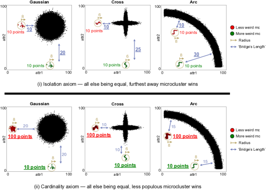
Figure 2: Proposed Axioms: the green microcluster is always more weird, i.e., larger anomaly score. All else being equal, (i) Isolation Axiom – furthest away microcluster wins; (ii) Cardinality Axiom – less populous microcluster wins. (best viewed in color)

IV Proposed Method

How could we have an outlier detector that works with a General Input (G1) and gives a General Output (G2) that is Principled (G3) in a Scalable (G4) and ‘Hands-Off’ (G5) way? Here we answer the question with McCatch. To our knowledge, it is the first method that achieves all of these five goals. We begin with the main intuition, and then detail our proposal.

IV-A Intuition & the ‘Oracle’ Plot

The high-level idea is to spot (i) points that are far from everything else (‘one-off’ outliers), and (ii) groups of points that form a microcluster, that is, they are close to each other, but far from the rest. The tough parts are how to quantify these intuitive concepts. We propose to use the new ‘Oracle’ plot.

‘Oracle’ plot

It focuses on plateaus formed in the count of neighbors of each point as the neighborhood radius varies. This idea is shown in Fig. 3. We present a toy dataset in 3(i), and its ‘Oracle’ plot in 3(ii). For easy of understanding, let us consider five points of interest: inlier ‘A’ in black; ‘halo-point’ ‘B’ in orange; ‘mc-point’ ‘C’ in green; ‘halo-mc-point’ ‘D’ in violet, and; ‘isolate-point’ ‘E’ in red. Our ‘Oracle’ plot groups inliers like ‘A’ at its bottom-left part. The other parts of the plot distinguish the outliers by type; see ‘B’, ‘C’, ‘D’, and ‘E’. Note that the outliers ‘C’ and ‘D’ that belong to the mc of green/violet points are isolated at the top part of the plot.

The details are in Fig.3(iii), where we plot the count of neighbors versus the radius for the points of interest. Each point is counted together with its neighbors, so the minimum count is $1$. The large, blue curves give the average count for the dataset. A plateau exists if the count of neighbors of a point remains (quasi) unaltered for two or more radii; let this count be the height of the plateau. The length of the plateau is the difference between its largest radius, and the smallest one. Note that the counts for each point of interest form at least two plateaus: the first plateau, and the last one, referring to small, and large radii respectively. Middle plateaus may also exist.

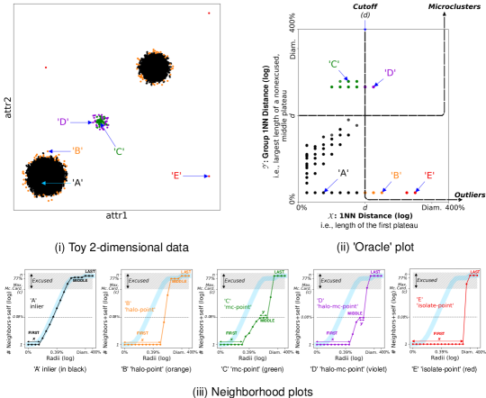
Figure 3: Intuition & the ‘Oracle’ plot: McCatch spots outliers in a dataset (i) using our ‘Oracle’ plot (ii). The plot groups inliers like point ‘A’ (in black) at its bottom-left, and distinguishes outliers by type; see ‘B’ (orange), ‘C’ (green), ‘D’ (violet), and ‘E’ (red). Outliers ‘C’ and ‘D’ from the microcluster in green/violet are isolated at the top. It is made possible by capitalizing on plateaus formed in the count of neighbors of each point as the neighborhood radius varies; see examples in (iii). (best viewed in color)

‘Plateaus’ correspond to clusters

In fact, the plateaus follow  a  hierarchical  clustering  structure.  Each  plateau  in  the

count of neighbors of a point describes this point’s cluster in one level of the hierarchy. This is why the first, and the last plateaus always exist: the first one regards a low level, where the point is a cluster of itself (or nearly so); the last plateau refers to a higher level where the point, and (nearly) all other points cluster together. Middle plateaus may be multiple, as the point may belong to clusters in many intermediary levels of the hierarchy. Note that a plateau shows: (i) the cluster’s cardinality, and; (ii) the cluster’s distance to other points. The plateau’s height is the cardinality; its length is the distance.

Examples of ‘plateaus’

The first plateaus in Fig. 3(iii) reveal that ‘A’ (in black) and ‘C’ (green) are close to their nearest neighbors, while ‘E’ (red) is isolated – see the length of each first plateau considering the log scale, and note the small lengths for ‘A’ and ‘C’, and the large one for ‘E’. The middle plateaus show that: (i) ‘A’ belongs to a populous, isolate cluster whose cardinality is $77\%$ of the dataset cardinality $n$ – see its middle plateau whose length is large, as well as the height that is also large, and; (ii) ‘C’ is part of an isolate mc whose cardinality is $0.08\%$ of $n$ – note that its middle plateau has a large length, but a small height. ‘E’ does not belong to any nonsingleton cluster due to the absence of a middle plateau.

Gory details: ‘excused’ plateaus and the ‘Oracle’ plot

Provided that we look for microclusters, we propose to excuse plateaus of large height; i.e., to ignore clusters of large cardinality, say, larger than a Maximum Microcluster Cardinality $c=\left\lceil{n\cdot 0.1}\right\rceil$. See the ‘Excused’ regions in the plots of Fig. 3(iii). Also, if any point happens to have two or more middle plateaus that are not excused, we only consider the one with the largest length, because the larger is the length of a plateau, the most isolated is the cluster that it describes. From now on, if we refer to a plateau, we mean a nonexcused plateau; and, if we refer to the middle plateau of a point, we mean this point’s nonexcused, middle plateau of largest length.

Our ‘Oracle’ plot is then built from the plateaus’ lengths. We plot for each point $\mathbf{p}_{i}$ the length $x_{i}$ of its first plateau versus the length $y_{i}$ of its middle plateau, using $y_{i}=0$ when $\mathbf{p}_{i}$ has no middle plateau. Importantly, $x_{i}$ is approximately the distance between $\mathbf{p}_{i}$ and its nearest neighbor. Let us refer to $x_{i}$ as the $\mathbf{1}$NN Distance of $\mathbf{p}_{i}$. On the other hand, $y_{i}$ is approximately the largest distance between any potential, nonsingleton mc that contains $\mathbf{p}_{i}$, and the nearest neighbor of this cluster. Thus, we refer to $y_{i}$ as the Group $\mathbf{1}$NN Distance of $\mathbf{p}_{i}$.

Hence, the ‘X’ axis of our ‘Oracle’ plot represents the possibility of each point to form a cluster of itself, that is, to be a singleton microcluster. If a point $\mathbf{p}_{i}$ is far from any other point, then $\mathbf{p}_{i}$ has a larger $x_{i}$ than it would have if it were close to another point. Distinctly, the ‘Y’ axis regards the possibility of each point to be in a nonsingleton microcluster. If $\mathbf{p}_{i}$ has a few close neighbors, i.e., fewer than $c$ neighbors, but it is far from other points, then $\mathbf{p}_{i}$ has a larger $y_{i}$ than it would have if its close neighbors were many, or none. Provided that $x_{i}$ and $y_{i}$ have both the same meaning – in the sense that each one is the distance between a potential microcluster $\mathbf{M}_{j}:\mathbf{p}_{i}\in\mathbf{M}_{j}$ and the cluster’s nearest neighbor – they can be compared to a threshold $d$ to verify if $\mathbf{p}_{i}$ is an outlier; i.e., if either $x_{i}$ or $y_{i}$ is larger than or equal to $d$. For instance, note in Fig. 3(ii) that a threshold $d$ distinguishes outliers and inliers. From now on, we refer to threshold $d$ as the Cutoff. McCatch obtains $d$ automatically, in a data-driven way, as we show later.

Algorithm 1 $\textsc{{McCatch}}\left(\ \ \right)$

Input Dataset $\mathbf{P}=\left\{\mathbf{p}_{1},\dots\mathbf{p}_{n}\right\}$;
         Number of Radii $a$; $\triangleright$ Default: $a=15$
         Maximum Plateau Slope $b$; $\triangleright$ Default: $b=0.1$
         Max. Mc. Cardinality $c$; $\triangleright$ Default: $c=\left\lceil{n\cdot 0.1}\right\rceil$
Output Microclusters $\mathcal{M}=\left\{\mathbf{M}_{1},\dots\mathbf{M}_{m}\right\}$;
           Scores per microcluster $\mathcal{S}=\left\{s_{1},\dots s_{m}\right\}$;
           Scores per point $\mathcal{W}=\left\{w_{1},\dots w_{n}\right\}$;

1:${\color[rgb]{1,0,0}\triangleright}$ Define the neighborhood radii

2:Build tree $\mathtt{T}$ for $\mathbf{P}$; $\triangleright$ Like a Slim-tree, M-tree, or R-treenote:tree

3:Estimate diameter $l$ of $\mathbf{P}$ from $\mathtt{T}$;

4:$\mathcal{R}=\left\{r_{1},r_{2},\dots r_{a}\right\}=\left\{\frac{l}{2^{a-1}},~{}\frac{l}{2^{a-2}},~{}\dots~{}\frac{l}{2^{0}}\right\}$;

5:${\color[rgb]{1,0,0}\triangleright}$ Build the ‘Oracle’ plot

6:$\mathtt{O}=\textsc{BuildOPlop}\left(\mathbf{P},\mathtt{T},\mathcal{R},b,c\right)$; $\triangleright$ Alg. 2

7:${\color[rgb]{1,0,0}\triangleright}$ Spot the microclusters

8:${\color[rgb]{0,0,1}\hskip 8.53581pt\triangleright}$ $\mathcal{M}=\{\mathbf{M}_{1},\dots\mathbf{M}_{m}\}$, where $\mathbf{M}_{j}\subset\mathbf{P}$

9:$\mathcal{M}=\textsc{SpotMCs}\left(\mathbf{P},\mathtt{O},\mathcal{R}\right)$; $\triangleright$ Alg. 3

10:${\color[rgb]{1,0,0}\triangleright}$ Compute the anomaly scores

11:${\color[rgb]{0,0,1}\hskip 8.53581pt\triangleright}$ $\mathcal{S}=\left\{s_{1},\dots s_{m}\right\}$, where $s_{j}$ refers to $\mathbf{M}_{j}$

12:${\color[rgb]{0,0,1}\hskip 8.53581pt\triangleright}$ $\mathcal{W}=\left\{w_{1},\dots w_{n}\right\}$, where $w_{i}$ refers to $\mathbf{p}_{i}$

13:$\mathcal{S},\mathcal{W}=\textsc{ScoreMCs}\left(\mathbf{P},\mathcal{M},\mathtt{O},\mathcal{R}\right)$; $\triangleright$ Alg. 4

14:return $\mathcal{M},\mathcal{S},\mathcal{W}$;

IV-B McCatch in a Nutshell

McCatch is shown in Alg. 1. Following the problem state-

ment from Probl. 1, it receives a dataset $\mathbf{P}=\left\{\mathbf{p}_{1},\dots\mathbf{p}_{n}\right\}$ as input, and returns a set of microclusters $\mathcal{M}=\left\{\mathbf{M}_{1},\dots\mathbf{M}_{m}\right\}$ together with their anomaly scores $\mathcal{S}=\left\{s_{1},\dots s_{m}\right\}$. For applications that require a full ranking of the points (as well as for backward compatibility with previous methods), McCatch also returns a set of scores per point $\mathcal{W}=\left\{w_{1},\dots w_{n}\right\}$, where $w_{i}\in\mathbb{R}_{>0}$ is the score of point $\mathbf{p}_{i}$.

Our method has hyperparameters, for which we provide reasonable default values: Number of Radii $a\in\mathbb{N}_{>1}$; Maximum Plateau Slope $b\in\mathbb{R}_{\geq 0}$, and; Maximum Microcluster Cardinality $c\in\mathbb{N}_{\geq 1}$. The default values $a=15$, $b=0.1$, and $c=\left\lceil{n\cdot 0.1}\right\rceil$ were used in every experiment reported in our paper. It confirms McCatch’s ability to be fully automatic.

In a nutshell, McCatch has four steps: (I) define neighborhood radii – see Lines $1$-$3$ in Alg. 1; (II) build ‘Oracle’ plot – Line $4$; (III) spot microclusters – Line $5$, and; (IV) compute anomaly scores – Line $6$. Step I is straightforward. We build a tree $\mathtt{T}$ for $\mathbf{P}$, like an R-tree, M-tree, or Slim-tree. Then, we estimate the diameter $l$ of $\mathbf{P}$ as the maximum distance between any child node (direct successor) of the root node of $\mathtt{T}$. Finally, we define the set of radii $\mathcal{R}=\left\{r_{1},\dots r_{a}\right\}=\left\{\frac{l}{2^{a-1}},~{}\frac{l}{2^{a-2}},~{}\dots~{}\frac{l}{2^{0}}\right\}$ to be used when counting neighbors. The next subsections detail Steps II, III, and IV.

IV-C Build the ‘Oracle’ Plot

Alg. 2 builds the ‘Oracle’ plot. It starts by counting neigh-

bors for each point w.r.t. a few radii of neighborhood – see Lines $1$-$3$. Specifically, for each radius $r_{e}\in\mathcal{R}$, we run a spatial self join algorithm $\textsc{SelfJoinC}\left(~{}\right)$ to obtain a set $\left\{q_{e}^{\left(1\right)},\dots q_{e}^{\left(n\right)}\right\}$, where $q_{e}^{\left(i\right)}$ is the count of neighbors (+ self) of $\mathbf{p}_{i}$ considering radius $r_{e}$. Any off-the-shelf spatial join algorithm can be used here. However: (i) the algorithm must be adapted to return only counts of neighbors, not pairs of neighboring points, and; (ii) we consider the use of any join algorithm that can leverage a tree $\mathtt{T}$ to speed up the process.

Later, we use $b$, $c$, and the counts $\left\{q_{1}^{\left(i\right)},\dots q_{a}^{\left(i\right)}\right\}$ of each point $\mathbf{p}_{i}$ to compute both the length $x_{i}$ of its first plateau, i.e., the $1$NN Distance, and the length $y_{i}$ of its middle plateau, i.e., the Group $1$NN Distance – see Lines $4$-$7$. The details are in Def.ns 1-3. Note that we use $x_{i}=0$ for every point $\mathbf{p}_{i}$ such that $q_{1}^{\left(i\right)}>1$, because, in these cases, the number of radii $a$ is not large enough to uncover the first plateau of that particular point. Similarly, we use $y_{i}=0$ for every point $\mathbf{p}_{i}$ that does not have a middle plateau. The plateau lengths are then employed in Lines $8$-$10$ to mount the ‘Oracle’ plot $\mathtt{O}=\left(\left\{x_{1},\dots x_{n}\right\},\left\{y_{1},\dots y_{n}\right\}\right)$, which is returned in Line $11$.

Definition 1 (Plateau)

A plateau $\mathtt{U}^{\left(i\right)}=\left[r_{e},r_{e^{\prime}}\right]$ of a point $\mathbf{p}_{i}$ is a maximal range of radii where the count of neighbors of $\mathbf{p}_{i}$ remains unaltered, or quasi-unaltered according to a Maximum Plateau Slope $b$. Formally, $\left[r_{e},r_{e^{\prime}}\right]$ is a plateau of $\mathbf{p}_{i}$ if and only if $r_{e},r_{e^{\prime}}\in\mathcal{R}$ with $r_{e}<r_{e^{\prime}}$, and the slope

$$\textsc{Slope}\left(e^{\prime\prime},~{}i\right)=\frac{\text{log}\left(q_{e^{\prime\prime}+1}^{\left(i\right)}\right)-\text{log}\left(q_{e^{\prime\prime}}^{\left(i\right)}\right)}{\text{log}\left(r_{e^{\prime\prime}+1}\right)-\text{log}\left(r_{e^{\prime\prime}}\right)}$$

is smaller than or equal to $b$ for every value $e^{\prime\prime}$, such that $r_{e^{\prime\prime}}\in\mathcal{R}$ and $e\leq e^{\prime\prime}<e^{\prime}$. Also, it must be true that: $\textsc{Slope}\left(e-1,~{}i\right)>b$, if $e>1$, and; $\textsc{Slope}\left(e^{\prime},~{}i\right)>b$, if $e^{\prime}<a$. The length of a plateau $\mathtt{U}^{\left(i\right)}=\left[r_{e},r_{e^{\prime}}\right]$ is given by $r_{e^{\prime}}-r_{e}$; its height is $q_{e}^{\left(i\right)}$, which must be smaller than, or equal to a Maximum Microcluster Cardinality $c$.

Definition 2 (First Plateau)

Among every plateau
$\mathtt{U}^{\left(i\right)}~{}=~{}\left[r_{e},r_{e^{\prime}}\right]$ of a point $\mathbf{p}_{i}$, the first plateau is the only one that has height one, that is, $q_{e}^{\left(i\right)}==1$. Let us use $\mathtt{X}^{\left(i\right)}$ to refer specifically to the first plateau of $\mathbf{p}_{i}$. Similarly, we use $x_{i}$ to denote the length of $\mathtt{X}^{\left(i\right)}$, which is the $\mathbf{1}$NN Distance of $\mathbf{p}_{i}$.

Definition 3 (Middle Plateau)

Among every plateau $\mathtt{U}^{\left(i\right)}=\left[r_{e},r_{e^{\prime}}\right]$ of $\mathbf{p}_{i}$ such that $r_{e^{\prime}}\neq l$ and $q_{e}^{\left(i\right)}>1$, the middle plateau is the one with the largest length $r_{e^{\prime}}-r_{e}$. We use $\mathtt{Y}^{\left(i\right)}$ to refer to the middle plateau of $\mathbf{p}_{i}$. Similarly, we use $y_{i}$ to denote the length of $\mathtt{Y}^{\left(i\right)}$, which is the Group $\mathbf{1}$NN Distance of $\mathbf{p}_{i}$.

IV-D Spot the Microclusters

Once the ‘Oracle’ plot is built, how to (i) spot the outliers, and then (ii) group the ones that are nearby each other? Alg. 3 gives the answers. It has two steps: to compute the Cutoff $d$ so to distinguish outliers from inliers as shown in Fig. 3(ii); and then, to gel the outliers into mcs, that is, to assign each outlying point to the correct cluster. The details are as follows.

Algorithm 2 $\textsc{BuildOPlot}\left(\ \ \right)$

Input Dataset $\mathbf{P}=\left\{\mathbf{p}_{1},\dots\mathbf{p}_{n}\right\}$;
         Tree $\mathtt{T}$;
         Radii $\mathcal{R}=\left\{r_{1},\dots r_{a}\right\}$;
         Maximum Plateau Slope $b$;
         Maximum Microcluster Cardinality $c$;
Output ‘Oracle’ plot $\mathtt{O}=\left(\left\{x_{1},\dots x_{n}\right\},\left\{y_{1},\dots y_{n}\right\}\right)$;

1:${\color[rgb]{1,0,0}\triangleright}$ Count the neighbors

2:${\color[rgb]{0,0,1}\hskip 8.53581pt\triangleright}$ $q_{e}^{\left(i\right)}=$ # neighbors (+ self) of $\mathbf{p}_{i}$ regarding radius $r_{e}$

3:for $e=1,\dots a$ do $\triangleright$ Run a join per radius

4:     $\left\{q_{e}^{\left(1\right)},\dots q_{e}^{\left(n\right)}\right\}=\textsc{SelfJoinC}\left(\mathtt{T},r_{e}\right)$;

5:end for

6:${\color[rgb]{1,0,0}\triangleright}$ Find the plateaus

7:for $\mathbf{p}_{i}\in\mathbf{P}$ do

8:${\color[rgb]{0,0,1}\hskip 25.60747pt\triangleright}$ Compute the $1$NN Distance

9:     $x_{i}=$ use $b$, $c$, and $\left\{q_{1}^{\left(i\right)},\dots q_{a}^{\left(i\right)}\right\}$ to compute

10:            the length of the first plateau of $\mathbf{p}_{i}$; $\triangleright$ Def. 2

11:     ${\color[rgb]{0,0,1}\hskip 8.53581pt\triangleright}$ Compute the Group $1$NN Distance

12:     $y_{i}=$ use $b$, $c$, and $\left\{q_{1}^{\left(i\right)},\dots q_{a}^{\left(i\right)}\right\}$ to compute

13:            the length of the middle plateau of $\mathbf{p}_{i}$; $\triangleright$ Def. 3

14:end for

15:${\color[rgb]{1,0,0}\triangleright}$ Mount the ‘Oracle’ plot

16:$\mathcal{X}=\left\{x_{1},\dots x_{n}\right\}$; $\triangleright$ ‘X’ axis

17:$\mathcal{Y}=\left\{y_{1},\dots y_{n}\right\}$; $\triangleright$ ‘Y’ axis

18:$\mathtt{O}=\left(~{}\mathcal{X},~{}\mathcal{Y}~{}\right)$; $\triangleright$ ‘Oracle’ plot

19:return $\mathtt{O}$;

Algorithm 3 $\textsc{SpotMCs}\left(\ \ \right)$

Input Dataset $\mathbf{P}=\left\{\mathbf{p}_{1},\dots\mathbf{p}_{n}\right\}$;
         ‘Oracle’ plot $\mathtt{O}=\left(\left\{x_{1},\dots x_{n}\right\},\left\{y_{1},\dots y_{n}\right\}\right)$;
         Radii $\mathcal{R}=\left\{r_{1},\dots r_{a}\right\}$;
Output Microclusters $\mathcal{M}=\left\{\mathbf{M}_{1},\dots\mathbf{M}_{m}\right\}$;

1:${\color[rgb]{1,0,0}\triangleright}$ Compute the Cutoff $d$

2:${\color[rgb]{0,0,1}\hskip 8.53581pt\triangleright}$ Build the Histogram of $1$NN Distances $\mathcal{H}$

3:$\mathcal{H}=\left\{h_{1},\dots h_{a}\right\}=\left\{0,\dots 0\right\}$;

4:for $\mathbf{p}_{i}\in\mathbf{P}$ do

5:     $e=e^{\prime}\in\left\{1,\dots a\right\}~{}:~{}x_{i}==r_{e^{\prime}}$; $\triangleright$ Find bin

6:     $h_{e}=h_{e}+1$; $\triangleright$ Count point $\mathbf{p}_{i}$ in bin $h_{e}$

7:end for

8:${\color[rgb]{0,0,1}\hskip 8.53581pt\triangleright}$ Data-driven computation of $d$

9:$d=$ use $\mathcal{H}$ and $\mathcal{R}$ to compute the Cutoff; $\triangleright$ Def. 6

10:${\color[rgb]{1,0,0}\triangleright}$ Gel the outliers into microclusters

11:$\mathbf{A}=\left\{\mathbf{p}_{i}\in\mathbf{P}:x_{i}\geq d\lor y_{i}\geq d\right\}$; $\triangleright$ All outliers

12:${\color[rgb]{0,0,1}\hskip 8.53581pt\triangleright}$ Gel nonsingleton microclusters

13:$\mathbf{M}=\{\mathbf{p}_{i}\in\mathbf{A}:y_{i}\geq d\}$; $\triangleright$ Large Group $1$NN Distance

14:Build tree $\mathtt{T}$ for $\mathbf{M}$;

15:$\overset{\uparrow}{x}~{}=~{}$max${}_{i}~{}x_{i}~{}:~{}\mathbf{p}_{i}\in\mathbf{M}$; $\triangleright$ Largest $1$NN Distance

16:$e~{}=~{}e^{\prime}\in\left\{1,\dots a\right\}~{}:~{}r_{e^{\prime}}==\overset{\uparrow}{x}$;

17:$\mathcal{E}=\textsc{SelfJoin}\left(\mathtt{T},r_{e+1}\right)$; $\triangleright$ Find neighbors

18:$\mathtt{G}~{}=~{}\left(~{}\mathbf{M},~{}\mathcal{E}~{}\right)$; $\triangleright$ Build neighborhood graph

19:$\mathtt{G}_{1},\dots\mathtt{G}_{m^{\prime}}=$ connected components of $\mathtt{G}$, where

20:              $\mathtt{G}_{j}=\left(\mathbf{M}_{j}\subseteq\mathbf{M},\mathcal{E}_{j}\subseteq\mathcal{E}\right)$; $\triangleright$ Find components

21:$\mathcal{M}=\{\mathbf{M}_{1},\dots\mathbf{M}_{m^{\prime}}\}$; $\triangleright$ Nonsingleton mcs

22:${\color[rgb]{0,0,1}\hskip 8.53581pt\triangleright}$ Gel singleton microclusters

23:for $\mathbf{p}_{i}\in\mathbf{A}\setminus\mathbf{M}$ do

24:     $\mathcal{M}=\mathcal{M}~{}\cup~{}\left\{\mathbf{p}_{i}\right\}$; $\triangleright$ Add singleton mc

25:end for

26:return $\mathcal{M}$;

IV-D1 Compute the Cutoff

How to let the data dictate the correct Cutoff? Ideally, we want a method which is hands-off without requiring any parameters. The first solution that comes to mind is $k$ standard deviations with $k$ equals $3$. Can we get rid of the $k$ parameter too?

Cutoff comes from compression: insight

Our insight is to use Occam’s razor [37] and formally the Minimum Description Length (MDL) [38]. MDL is a powerful way of regularizing and eliminating the need for parameters. The idea is to choose those parameter values that result in the best compression of the given dataset. It is a well respected principle made popular by Jorma Rissanen [38], Peter Grünwald [37] and others.

We compute the Cutoff $d$ by capitalizing on the set $\left\{x_{1},\dots x_{n}\right\}$ of $1$NN Distances; that is, by leveraging the ‘X’ axis of our ‘Oracle’ plot. Importantly, it is expected that many points have small values in this axis, while only a few points have larger values. The small values come mostly from inliers, such as the black point ‘A’ in Fig 3(i), but a few ones may come from outliers in the core of a non-singleton microcluster, like point ‘C’ in green, because these points also have close neighbors. Distinctly, larger values derive exclusively from outliers, e.g., ‘B’ (in orange), ‘D’ (violet) and ‘E’ (red). It allows us to compute $d$ in a data-driven way, by partitioning a histogram of $1$NN Distances so to best separate the tall bins that refer to small distances from the short bins that regard large distances. Intuitively, Cutoff $d$ is the minimum distance required between one microcluster and its nearest inlier.

Fig. 4 shows how we compute $d$. At the bottom, it presents the ‘X’ axis projection of the ‘Oracle’ plot shown in Fig. 3(ii). Note that the positioning of points ‘A’ (in black), ‘B’ (orange), ‘C’ (green), ‘D’ (violet) and ‘E’ (red) reflects the discussion of the previous paragraph. The corresponding histogram of points is shown in the central part of Fig. 4. We refer to it as the Histogram of $\mathbf{1}$NN Distances. As expected, the majority of the points is counted in bins referring to small distances in the histogram – see the tall bins on its left side. The Cutoff $d$ is the distance that best separates the tall bins from the short ones, where the former refer to small distances and the latter regard large distances. We obtain it automatically from the data, by partitioning the Histogram of $1$NN Distances so to minimize the cost of compressing the partitions – see the top part of Fig. 4. Besides being parameter-free, our solution is grounded in the same concept of compression used later to generate scores, and, thus, it increases the coherence of our method.

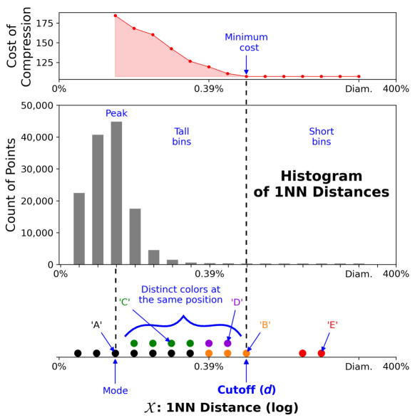
Figure 4: McCatch obtains the Cutoff $\mathbf{d}$ automatically, by partitioning a histogram of $1$NN Distances so to best separate tall and short bins. It is done by minimizing the cost of compressing the partitions. (best viewed in color)

Cutoff comes from compression: details

Here we provide

the details of computing $d$. As shown in Lines $1$-$5$ of Alg. 3, we follow Def. 4 to build the Histogram of $1$NN Distances $\mathcal{H}=\left\{h_{1},\dots h_{a}\right\}$. Then, in Line $6$, we use Def.ns 5-6 to obtain $d$. Specifically, we find the peak bin $h_{e^{\prime}}$. It regards the distance/radius $r_{e^{\prime}}$ most commonly seen between a point and its nearest neighbor. Obviously, $d$ must be larger than $r_{e^{\prime}}$. Hence, we compute $d$ considering only the bins in $\left\{h_{e^{\prime}},\dots h_{a}\right\}$. They are analyzed to find the best cut position $e$ that maximizes the homogeneity of values in subsets $\left\{h_{e^{\prime}},\ldots h_{e-1}\right\}$ and $\left\{h_{e},\ldots h_{a}\right\}$, so to best separate the tall from the short bins.

Definition 4 (Histogram of $\mathbf{1}$NN Distances)

The Histogram of $1$NN Distances is defined as a set $\mathcal{H}~{}=~{}\left\{h_{1},\dots h_{a}\right\}$, in which each bin $h_{e}$ is computed as follows: $h_{e}~{}=~{}\mid\left\{\mathbf{p}_{i}\in\mathbf{P}~{}:~{}x_{i}==r_{e}\right\}\mid$.

Definition 5 (Cost of Compression)

The cost of compression of a nonempty set $\mathcal{V}\subset\mathbb{N}_{\geq 0}$ with average $\overset{-}{v}$ is

$$\textsc{Cost}\left(\mathcal{V}\right)= \bigl{<}\mid\mathcal{V}\mid\bigr{>}+\biggl{<}1+\left\lceil{\overset{-}{v}}\right\rceil\biggr{>}+\sum_{v\in\mathcal{V}}\biggl{<}1+\left\lceil{\mid v-\overset{-}{v}\mid}\right\rceil\biggr{>}$$

, where $\bigl{<}~{}\bigr{>}$ is the universal code length for integers.

Definition 6 (Cutoff)

The Cutoff $d$ is defined as

$$d~{}=~{}r_{e}\in\mathcal{R}~{}:~{}e~{}\text{minimizes}~{} \textsc{Cost}\left(\left\{h_{e^{\prime}},\ldots h_{e-1}\right\}\right)+$$

$$\textsc{Cost}\left(\left\{h_{e},\ldots h_{a}\right\}\right)$$

, where $\left\{h_{e^{\prime}},\ldots h_{e-1}\right\}$ and $\left\{h_{e},\ldots h_{a}\right\}$ are subsets of $\mathcal{H}$, and $e^{\prime}$ is chosen so that radius $r_{e^{\prime}}\in\mathcal{R}$ is the mode of $\left\{x_{1},\dots x_{n}\right\}$.

To obtain $e$, based on the principle of MDL, we check partitions $\left\{h_{e^{\prime}},\ldots h_{e^{\prime\prime}-1}\right\}$ and $\left\{h_{e^{\prime\prime}},\ldots h_{a}\right\}$ for all possible cut positions $e^{\prime\prime}$. The idea is to compress each possible partition, representing it by its cardinality, its average, and the differences of each of its values to the average. A partition with high homogeneity of values allows good compression, as its differences to the average are small, and small numbers need less bits to be represented than large ones do. The best cut position $e$ is, therefore, the one that creates the partitions that compress best. Note in Def. 5 that we add ones to some values whose code lengths $\bigl{<}~{}\bigr{>}$ are required, so to account for zeros. Cutoff $d$ is then obtained as $d=r_{e}$, without depending on any input from the user. It allows us to identify the set $\mathbf{A}=\left\{\mathbf{p}_{i}\in\mathbf{P}~{}:~{}x_{i}\geq d~{}\lor~{}y_{i}\geq d\right\}$ of all outliers.

IV-D2 Gel the outliers into microclusters

Given the outliers, how to cluster them? Alg. 3 provides the answer. We use the ‘Y’ axis of the ‘Oracle’ plot to isolate outliers of nonsingleton mcs into a set $\mathbf{M}=\{\mathbf{p}_{i}\in\mathbf{A}:y_{i}\geq d\}$; see Line $8$. Then, in Lines $9$-$15$, we group these points using the plot’s ‘X’ axis. Every outlier in $\mathbf{M}$ must be grouped together with its nearest neighbor; thus, we identify the largest $1$NN Distance $\overset{\uparrow}{x}~{}=~{}\text{max}_{i}~{}x_{i}:\mathbf{p}_{i}\in\mathbf{M}$, and use it to specify a threshold that rules if each possible pair of points from $\mathbf{M}$ is close enough to be grouped together. Provided that the $1$NN Distances are approximations, the threshold itself is the smallest radius larger than $\overset{\uparrow}{x}$, that is, radius $r_{e+1}$ from Line $12$. It avoids having a point and its nearest neighbor in distinct clusters.

The nonsingleton mcs are then identified by spotting connected components in a graph $\mathtt{G}~{}=~{}\left(~{}\mathbf{M},~{}\mathcal{E}~{}\right)$, where $\mathbf{M}$ is the set of nodes, and $\mathcal{E}\subseteq\mathbf{M}\times\mathbf{M}$ is the set of edges. The edges are obtained from any off-the-shelf spatial self join algorithm $\textsc{SelfJoin}\left(~{}\right)$ that returns pairs of nearby points from $\mathbf{M}$ – see Line $12$. Lastly, in Lines $16$-$19$, we recognize each outlier in $\mathbf{A}\setminus\mathbf{M}$ as a cluster of itself, and return the final set of mcs $\mathcal{M}$.

IV-E Compute the Anomaly Scores

Given the mcs, how to get scores that obey our axioms?

Scores come from compression: insight

We quantify the anomalousness of each mc according to how much it can be compressed when described in terms of the nearest inlier. Fig. 5 depicts this idea. To describe a microcluster $\mathbf{M}_{j}$ we would store its cardinality $\mid\mathbf{M}_{j}\mid$ and the identifier $i\in\left\{1,2,\dots n\right\}$ of the nearest inlier $\mathbf{p}_{i}$. See Items ① and ② in Fig. 5. Then, we would use $\mathbf{p}_{i}$ as a reference to describe the point $\mathbf{p}_{i^{\prime}}\in\mathbf{M}_{j}$ that is the closest to it. To this end, we would store the differences (e.g., in each feature if we have vector data) between $\mathbf{p}_{i}$ and $\mathbf{p}_{i^{\prime}}$; see ③. Point $\mathbf{p}_{i^{\prime}}$ would in turn be the reference to describe its nearest neighbor $\mathbf{p}_{i^{\prime\prime}}\in\mathbf{M}_{j}$, which would later serve as a reference to describe one other close neighbor from $\mathbf{M}_{j}$, thus following a recursive process that would lead us to describe every point of $\mathbf{M}_{j}$; see ④. Importantly, in this representation, the cost per point – that is, the total number of bits used to describe $\mathbf{M}_{j}$ divided by $\mid\mathbf{M}_{j}\mid$ – reflects the axioms of Fig. 2. A large ‘Bridge’s Length’ increases the cost per point due to ③. Also, the larger the cardinality, the smaller the cost per point. It is because the costs of ①, ② and ③ are diluted with points. Hence, the cost per point appropriately quantifies the anomalousness of $\mathbf{M}_{j}$.

Scores come from compression: details

Alg. 4 computes the scores. We begin by finding the ‘Bridge’s Length’ $\overset{\downarrow}{g}\overset{{\left(j\right)}}{}$ of each $\mathbf{M}_{j}$. To this end, we compute the distance $g_{i}$ between each outlier $\mathbf{p}_{i}\in\mathbf{A}$ and its nearest inlier; see Lines $1\text{-}12$. Specifically, we run a join between $\mathbf{A}$ and $\mathbf{P}\setminus\mathbf{A}$ for each $r_{e}\in\mathcal{R}$. Any spatial join algorithm can be used here, but it must be adapted to return counts of neighbors, not pairs of points. Each $g_{i}$ is then the largest radius for which $\mathbf{p}_{i}$ has zero neighbors. The ‘Bridge’s Length’ $\overset{\downarrow}{g}\overset{{\left(j\right)}}{}$ is finally found for each $\mathbf{M}_{j}$ in Line $17$; it is the smallest distance $g_{i}:\mathbf{p}_{i}\in\mathbf{M}_{j}$.

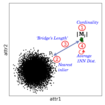
Figure 5: McCatch’s scores quantify how much each mc $\mathbf{M}_{j}$ is compressed when it is described in terms of the nearest inlier $\mathbf{p}_{i}$. (best viewed in color)

Definition 7 (Score)

The score $s_{j}$ of $\mathbf{M}_{j}$ is defined as

$$s_{j}~{}=~{}\frac{\text{{\color[rgb]{1,0,0}\Large\char 172}}~{}~{}\raisebox{2.0pt}{$+$}~{}~{}\text{{\color[rgb]{1,0,0}\Large\char 173}}~{}~{}\raisebox{2.0pt}{$+$}~{}~{}\text{{\color[rgb]{1,0,0}\Large\char 174}}~{}~{}\raisebox{2.0pt}{$+~{}~{}\left(\mid\mathbf{M}_{j}\mid-1\right)\cdot$}~{}\text{{\color[rgb]{1,0,0}\Large\char 175}}}{\mid\mathbf{M}_{j}\mid}$$

where

① $$=~{}\bigl{<}~{}\mid\mathbf{M}_{j}\mid~{}\bigr{>}\text{{\color[rgb]{0,0,1}\hskip 119.50157pt\hfill$\triangleright$ Cardinality}}$$

② $$=~{}\bigl{<}~{}n~{}\bigr{>}\text{{\color[rgb]{0,0,1}\hskip 133.72795pt\hfill$\triangleright$ Nearest inlier}}$$

③ $$=~{}t~{}\cdot~{}\Biggl{<}~{}\frac{\overset{\downarrow}{g}\overset{{\left(j\right)}}{}}{r_{1}}~{}\Biggr{>}\text{{\color[rgb]{0,0,1}\hskip 82.51299pt\hfill$\triangleright$ `Bridge's Length'}}$$

④ $$=~{}t~{}\cdot~{}\Biggl{<}~{}1~{}+~{}\left\lceil{\frac{\overset{-}{x}\overset{{\left(j\right)}}{}}{r_{1}}}\right\rceil~{}\Biggr{>}\text{{\color[rgb]{0,0,1}\hskip 18.49428pt\hfill$\triangleright$ Average {$1$NN Distance}}}$$

with $\overset{-}{x}\overset{{\left(j\right)}}{}=\text{avg}_{i}~{}x_{i}:\mathbf{p}_{i}\in\mathbf{M}_{j}$. The Transformation Cost $t$ is

$$t=\begin{cases}\text{Data dimensionality}&\text{, if {vector space}}\vspace{0.1in}\\ \bigl{<}3\bigr{>}+\bigl{<}\text{\# distinct chars.}\bigr{>}&\text{, if {words using}}\\ +~{}\bigl{<}\text{\# chars. longest word}\bigr{>}&\text{{edit distance}}\vspace{0.1in}\\ \text{Cost to transform a point into another}&\text{, if {other space}}\\ \text{point that is one unit of distance away}&\end{cases}$$

and $\bigl{<}~{}\bigr{>}$ is the universal code length for integersnote:logstar.

After that, we follow suit with the idea of Fig. 5 and compute the scores using Def. 7. Item ① in Def. 7 is the cost of storing the cardinality $\mid\mathbf{M}_{j}\mid$. Item ② is the cost of storing the identifier $i\in\left\{1,2,\dots n\right\}$ of the nearest inlier $\mathbf{p}_{i}$. We always consider the worst-case scenario here (that is, when $i=n$) to standardize the cost and also to avoid any dependence on the order of points in $\mathbf{P}$. Item ③ reflects the cost of storing the differences between $\mathbf{p}_{i}$ and the point $\mathbf{p}_{i^{\prime}}\in\mathbf{M}_{j}$ that is the closest to it. To work with vector and nondimensional data, we approximate this cost using the distance between $\mathbf{p}_{i}$ and $\mathbf{p}_{i^{\prime}}$, which is $\overset{\downarrow}{g}\overset{{\left(j\right)}}{}$; it is then normalized using $r_{1}$. We also use the Transformation Cost $t$ of the metric space; i.e., the cost to transform a point into another point that is one unit of distance away. For example, in a vector space, $t$ is the dimensionality because we must know the differences between $\mathbf{p}_{i}$ and $\mathbf{p}_{i^{\prime}}$ in each one of the features. As for another example, when analyzing words using the edit distance, $t$ is the cost of describing: (i) the transformation to be performed, among the three options insertion, deletion and replacement; (ii) the new character to be inserted or to replace the existing one, and; (iii) the position where the transformation must occur. Finally, Item ④ refers to the cost of storing the differences between each one of the remaining $\mid\mathbf{M}_{j}\mid-1$ points to be described and its point of reference. The cost is once more approximated using distances to work with any metric data.

For applications requiring a full ranking of the points (and for backward compatibility with other methods), we also have a score $w_{i}$ for each $\mathbf{p}_{i}$. To this end, we follow previous ideas and propose a score representing the cost of describing $\mathbf{p}_{i}$ in terms of the nearest inlier; see Lines $13$-$15$ and $21$-$24$ in Alg. 4.

IV-F Time and Space Complexity

Lemma 1 (Time Complexity)

The time complexity of McCatch is $O\left(n~{}\cdot~{}n^{1-\frac{1}{u}}\right)$, where $u$ is the intrinsic (correlation fractal) dimension of $\mathbf{P}$.

Proof 1

McCatch is presented in Alg. 1. It builds a tree $\mathtt{T}$ for $\mathbf{P}$ in $O\left(n~{}\cdot~{}\text{log}\left(n\right)\right)$ time, and then computes $l$ and $\mathcal{R}$ in a negligible time. Later, it spots microclusters by calling functions $\textsc{BuildOPlot}\left(\ \ \right)$ from Alg. 2, $\textsc{SpotMCs}\left(\ \ \right)$ from Alg. 3 and $\textsc{ScoreMCs}\left(\ \ \right)$ from Alg. 4, sequentially. Therefore, the overall cost of McCatch is the larger between $O\left(n~{}\cdot~{}\text{log}\left(n\right)\right)$ and the costs of Algs. 2, 3 and 4.

Alg. 2 counts neighbors by running $a$ self-joins for $\mathbf{P}$. Because $a$ is small, the complexity of this step is the same as that of one single self-join. The self-join finds neighbors for each of $n$ points. A rough, upper-bound estimation for its runtime is thus $O\left(n\cdot\textsc{NN}\left(n\right)\right)$, where $\textsc{NN}\left(n\right)$ is time taken by each nearest neighbor search. According to Pagel, Korn and Faloutsos [41], $\textsc{NN}\left(n\right)=O\left(n^{1-\frac{1}{u}}\right)$, in which $u$ is the intrinsic (correlation fractal) dimension of a vector dataset $\mathbf{P}$. For nondimensional data, Traina Jr. et al. [35] demonstrate that the query cost also depends on $u$. It leads us to estimate the cost of counting neighbors as $O\left(n~{}\cdot~{}n^{1-\frac{1}{u}}\right)$. Later, Alg. 2 finds plateaus in $O\left(n\right)$ time, and then it mounts $\mathtt{O}$ in a negligible time. Hence, the cost of Alg. 2 is $O\left(n~{}\cdot~{}n^{1-\frac{1}{u}}\right)$.

Algs. 3 and 4 scan $\mathbf{P}$ in $O\left(n\right)$ time. They also process the set of outliers $\mathbf{A}$, which takes a negligible time because $\mid\mathbf{A}\mid$ is small. Thus, the time required by each algorithm is $O\left(n\right)$.

As the total cost is the larger between $O\left(n~{}\cdot~{}\text{log}\left(n\right)\right)$ and the costs of Algs. 2, 3 and 4, it comes to $O\left(n~{}\cdot~{}n^{1-\frac{1}{u}}\right)$. We consider $u>1$ because it is the most expected scenario. $\blacksquare$

Note

In our experience, real data often have fractal dimension $u$ smaller than $20$ [41, 42]. As shown in [35], several nondimensional data have small $u$. Thus, McCatch should be subquadratic on the count of points for most real applications.

Lemma 2 (Space Complexity)

The space complexity of
McCatch is given by $O\left(n\right)$.

Proof 2

McCatch receives a set $\mathbf{P}$ as the input, and returns sets $\mathcal{M}$, $\mathcal{S}$ and $\mathcal{W}$ as the output. The largest data structures employed to this end are the ‘Oracle’ plot $\mathtt{O}$ and a tree $\mathtt{T}$ created for $\mathbf{P}$ in Alg. 1. $\mathbf{P}$, $\mathcal{W}$, $\mathtt{O}$ and $\mathtt{T}$ require $O\left(n\right)$ space each. $\mathcal{M}$ and $\mathcal{S}$ have negligible space requirements, as they require $O\left(\mid\mathbf{A}\mid\right)$ space with a small $\mid\mathbf{A}\mid$. Consequently, the space complexity of McCatch is $O\left(n\right)$. $\blacksquare$

Algorithm 4 $\textsc{ScoreMCs}\left(\ \ \right)$

Input Dataset $\mathbf{P}=\left\{\mathbf{p}_{1},\dots\mathbf{p}_{n}\right\}$;
         Microclusters $\mathcal{M}=\left\{\mathbf{M}_{1},\dots\mathbf{M}_{m}\right\}$;
         ‘Oracle’ plot $\mathtt{O}=\left(\left\{x_{1},\dots x_{n}\right\},\left\{y_{1},\dots y_{n}\right\}\right)$;
         Radii $\mathcal{R}=\left\{r_{1},\dots r_{a}\right\}$;
Output Scores per microcluster $\mathcal{S}=\left\{s_{1},\dots s_{m}\right\}$;
           Scores per point $\mathcal{W}=\left\{w_{1},\dots w_{n}\right\}$;

1:${\color[rgb]{1,0,0}\triangleright}$ Compute the distances to the nearest inliers

2:${\color[rgb]{0,0,1}\hskip 8.53581pt\triangleright}$ For outliers

3:$\mathbf{A}=\bigcup_{j=1}^{m}\mathbf{M}_{j}$; $\triangleright$ All outliers

4:Build tree $\mathtt{T}$ for $\mathbf{A}$; $\triangleright$ Tree for outliers

5:Build tree $\mathtt{T^{\prime}}$ for $\mathbf{P}\setminus\mathbf{A}$; $\triangleright$ Tree for inliers

6:for $e=1,\dots a$ do

7:${\color[rgb]{0,0,1}\hskip 25.60747pt\triangleright}$ $f_{e}^{\left(i\right)}=$ # of neighboring inliers of $\mathbf{p}_{i}$ w.r.t. $r_{e}$

8:     $\left\{f_{e}^{\left(i\right)}:\mathbf{p}_{i}~{}\text{in}~{}\mathtt{T}\right\}=\textsc{JoinC}\left(\mathtt{T},\mathtt{T^{\prime}},r_{e}\right)$; $\triangleright$ Join

9:     for $\mathbf{p}_{i}$ in $\mathtt{T}$ do

10:         if $f_{e}^{\left(i\right)}>0$ then

11:              $g_{i}=r_{e-1}$; $\triangleright$ $g_{i}=$ distance to nearest inlier

12:              Remove $\mathbf{p}_{i}$ from $\mathtt{T}$;

13:         end if

14:     end for

15:end for

16:${\color[rgb]{0,0,1}\hskip 8.53581pt\triangleright}$ For inliers

17:for $\mathbf{p}_{i}\in\mathbf{P}\setminus\mathbf{A}$ do

18:     $g_{i}=x_{i}$; $\triangleright$ $g_{i}$ is the $1$NN Distance of $\mathbf{p}_{i}$

19:end for

20:${\color[rgb]{1,0,0}\triangleright}$ Compute the scores per microcluster

21:for $\mathbf{M}_{j}\in\mathcal{M}$ do

22:     $\overset{\downarrow}{g}\overset{{\left(j\right)}}{}=\text{min}_{i}~{}g_{i}:\mathbf{p}_{i}\in\mathbf{M}_{j}$; $\triangleright$ ‘Bridge’s Length’

23:     $s_{j}=$ use $\mathbf{M}_{j}$, $\mathcal{R}$, $\mathtt{O}$, $\overset{\downarrow}{g}\overset{{\left(j\right)}}{}$ to get score of $\mathbf{M}_{j}$; $\triangleright$ Def. 7

24:end for

25:$\mathcal{S}=\left\{s_{1},\dots,s_{m}\right\}$; $\triangleright$ Set of scores per microcluster

26:${\color[rgb]{1,0,0}\triangleright}$ Compute the scores per point

27:for $\mathbf{p}_{i}\in\mathbf{P}$ do

28:     $w_{i}=\Bigl{<}1+\frac{g_{i}}{r_{1}}\Bigr{>}$; $\triangleright$ $\bigl{<}~{}\bigr{>}$ is the code length for integersnote:logstar

29:end for

30:$\mathcal{W}=\left\{w_{1},\dots,w_{n}\right\}$; $\triangleright$ Set of scores per point

31:return $\mathcal{S},\mathcal{W}$;

IV-G Implementation

The main cost of McCatch regards counting neighbors to build the ‘Oracle’ plot. As shown in Lines $1$-$3$ of Alg. 2, we can count neighbors using a didactic strategy that is easy to follow. Nevertheless, when using this strategy, we count the neighbors of every point w.r.t. all radii, which is unnecessary because we only need a count $q_{e}^{\left(i\right)}$ if it is smaller than or equal to $c$; see the ‘Excused’ regions in Fig. 3(iii). Our actual implementation follows a sparse-focused, speed-up principle:

• Sparse-focused principle: run a self-join for $\mathbf{P}$ with $r_{1}$. Then, for each $r_{e}\in\left\{r_{2},\dots r_{a}\right\}$, from smallest to largest, run a join (not self) between $\left\{\mathbf{p}_{i}\in\mathbf{P}~{}:~{}q_{e-1}^{\left(i\right)}\leq c\right\}$ and $\mathbf{P}$, thus computing only the counts required.

Other speed-up principles we employ for joins are:

• Count-only principle: do not materialize pairs of neighbors (e.g., by leveraging ‘compact similarity joins’ [43]) because we only need counts of neighbors, not the actual pairs of points. It applies to the joins in Algs. 2 and 4.

• Using-index principle: use a tree, like an R-tree, M-tree, or Slim-treenote:tree. It applies to the joins in Algs. 2, 3 and 4.

• Small-radii-only principle: don’t run a join for radius $r_{a}$. Since $r_{a}=l$, we already know all points are neighbors of each other. It applies to the joins in Algs. 2, 3 and 4.

V Experiments

We designed experiments to answer five questions:

1. Accurate: How accurate is McCatch?

2. Principled: Does McCatch obey axioms?

3. Scalable: How scalable is McCatch?

4. Practical: How well McCatch works on real data?

5. ‘Hands-Off’: Does McCatch need manual tuning?

Setup, code, competitors, and datasets

McCatch was coded in Java and C$++$. The joins in Algs. 2-4 employ the approach of ‘compact similarity joins’ [43].

We compared McCatch with $11$ state-of-the-art competitors: ABOD, FastABOD, LOCI, ALOCI, DB-Out, LOF, iForest and ODIN, which are coded in Java under the framework ELKI (elki-project.github.io), besides; Gen2Out, D.MCA and RDA whose original source codes in Python were used. Tab. II has the hyperparameter values employed. McCatch was always tested with its default configurationnote:sensitivity. The competitors were carefully tuned following hyperparameter-setting heuristics widely adopted in prior works, such as in [18, 6, 44, 21, 45, 5, 4, 2, 19, 28]. Non-deterministic competitors were run $10$ times per dataset; we report the average results.

TABLE II: Hyperparameter configuration.

Method	Values used
ALOCI	$g\in\{10,~{}15,~{}20\}$,  $nmin=20$,  $\alpha=4$
DB-Out	$r\in\{l\cdot 0.05,~{}l\cdot 0.1,~{}l\cdot 0.25,~{}l\cdot 0.5\}$
D.MCA	$\psi\in\{2,~{}4,~{}8,~{}\dots~{}\text{min}(1,024,~{}n\cdot 0.3)\}$,
	$t\in\{2,~{}4,~{}8,~{}\dots~{}128\}$,  $p=n\cdot 0.1$
FastABOD	$k\in\{1,~{}5,~{}10\}$
Gen2Out	$lb=1$,  $ub=11$,  $md\in\{2,3\}$,  $t\in\{2,~{}4,~{}8,~{}\dots~{}128\}$
iForest	$t\in\{2,~{}4,~{}8,~{}\dots~{}128\}$,  $\psi\in\{2,~{}4,~{}8,~{}\dots~{}\text{min}(1,024,~{}n\cdot 0.3)\}$
LOCI	$r\in\{l\cdot 0.05,~{}l\cdot 0.1,~{}l\cdot 0.25,~{}l\cdot 0.5\}$,  $nmin=20$,  $\alpha=0.5$
LOF	$k\in\{1,~{}5,~{}10\}$
ODIN	$k\in\{1,~{}5,~{}10\}$
RDA	$nlayers\in\{2,~{}3,~{}4\}$,  $dimdecay\in\{1,~{}2,~{}4\}$,
	$niter\in\{20,~{}50\}$,  $\lambda\in\{10e-5,~{}7.5e-5,~{}10e-4\}$
McCatch	$a=15$,  $b=0.1$,  $c=\left\lceil{n\cdot 0.1}\right\rceil$

Tab. III summarizes our data, which we describe as follows:

• Last Names: $5k$ names of people frequent in the US (inliers), and $50$ names frequent elsewhere (outliers).

• Fingerprints: ridges from $398$ full (inliers) and $10$ partial (outliers) fingerprints.

• Skeletons: skeleton graphs from $200$ human (inliers) and $3$ wild-animal (outliers) silhouettes.

• Axioms: synthetic data with Gaussian-, cross- and arc-shaped inliers following each axiom as shown in Fig. 2.

• Popular benchmark datasets: benchmark data from many real domains. Importantly, HTTP and Annthyroid are known to have nonsingleton microclusters [6].

• Shanghai and Volcanoes: average RGB values extracted from satellite image tiles. Outliers are unknown.

• Uniform and Diagonal: $2$-, $4$-, $20$-, and $50$-dim. data that follow a uniform distribution, or form a diagonal line.

In all cases we have that (i) for vector data, we use the Eu- clidean distance (but any other $L_{p}$ metric would work), and (ii) for nondimensional datasets the distance function is given by a domain expert. For example, string-editing or soundex encoding distance[46] for strings, and mathematical morphology[47] or tree-editing distance[48] for shapes or skeleton graphs.

TABLE III: Summary of datasets.

	Dataset	# Points	# Features (Emb. Dim.)	Intrinsic (Fractal) Dim.	% Outliers
Non-dim.	Last Names	$5,050$	–	$5.3$	$2.22$
	Fingerprints	$408$	–	$8.0$	$2.45$
	Skeletons	$203$	–	$2.1$	$1.47$
Axs.	Gauss., Cross, Arc (Isolation Ax.)	$\sim 1$ million	$2$	$1.7$	$0.002$
	Gauss., Cross, Arc (Cardinality Ax.)	$\sim 1$ million	$2$	$1.7$	$0.01$
Popular Benchmark Datasets	HTTP	$222,027$	$3$	$1.2$	$0.03$
	Shuttle	$49,097$	$9$	$1.8$	$7.15$
	kddcup08	$24,995$	$25$	$3.6$	$0.68$
	Mammography	$7,848$	$6$	$1.4$	$3.22$
	Annthyroid	$7,200$	$6$	$1.8$	$7.41$
	Satellite	$6,435$	$36$	$3.0$	$31.64$
	Satimage2	$5,803$	$36$	$3.0$	$1.22$
	Speech	$3,686$	$400$	$5.9$	$1.65$
	Thyroid	$3,656$	$6$	$0.7$	$2.54$
	Vowels	$1,452$	$12$	$0.8$	$3.17$
	Pima	$526$	$8$	$2.2$	$4.94$
	Ionosphere	$350$	$33$	$1.6$	$35.71$
	Ecoli	$336$	$7$	$1.9$	$2.68$
	Vertebral	$240$	$6$	$1.9$	$12.5$
	Glass	$213$	$9$	$1.3$	$4.23$
	Wine	$129$	$13$	$2.3$	$7.75$
	Hepatitis	$70$	$20$	$1.5$	$4.29$
	Parkinson	$50$	$22$	$1.4$	$4$
Sat.	Volcanoes	$3,721$	$3$	$1.8$	Unknown
	Shanghai	$1,296$	$3$	$1.4$	Unknown
Synt.	Uniform	$1$ million	$\left[2,50\right]$	$\left[2.0,50.0\right]$	$0$
	Diagonal	$1$ million	$\left[2,50\right]$	$1.0$	$0$

Figure 6: Q1. McCatch is Accurate and typically beats competition (red): Accuracy comparison. Top: McCatch wins in vector data with known non-singleton microclusters, and also in nondimensional data. Bottom: our method ties with the competitors in other cases. (best viewed in color)

Figure 7: Q3. McCatch is Scalable: Runtime vs. data size. Lines show expected slopes (Lemma 1). Estimations and measurements agree very well: McCatch is subquadratic in all cases, despite embedding dimension. Note: Uniform in (iii) and (iv) have respectively fractal dimension $\mathit{20}$ and $\mathit{50}$!

V-A Q1. McCatch is Accurate

Fig. 6 reports results regarding the accuracy of McCatch. For every dataset where outliers are known, we compare the Area Under the Receiver Operator Characteristic curve (AUROC) obtained by McCatch with that of each competitor. All methods were evaluated according to the anomaly scores they reported per point. Note that it was unfeasible to run D.MCA, ABOD, FastABOD, DB-Out and LOCI in some datasets; they either required an excessive runtime (i.e., $>10$ hours) or an excessive RAM memory usage (i.e., $>30$ GB). These two cases are respectively denoted by symbols  and .

TABLE IV: Accuracy Evaluation

	ABOD	ALOCI	DB-Out	D.MCA	FastABOD	Gen2Out	iForest	LOCI	LOF	ODIN	RDA	McCatch
H. Mean Rank (AUROC)	$2.2$	$4.6$	$5.1$	$4.4$	$2.8$	$2.8$	$3.5$	$6.0$	$4.9$	$4.9$	$3.6$	$1.8$
H. Mean Rank (AP)	$2.5$	$5.2$	$5.5$	$4.8$	$2.8$	$2.6$	$3.0$	$6.1$	$3.6$	$4.7$	$2.8$	$2.3$
H. Mean Rank (Max-F1)	$2.8$	$4.3$	$4.5$	$5.0$	$2.5$	$3.9$	$3.0$	$5.4$	$2.8$	$3.7$	$6.5$	$1.8$

Tab. IV reports the harmonic mean of the ranking positions of each method over all datasets. Besides AUROC, we consider additional metrics: Average Precision (AP) and Max-F1. McCatch outperforms every competitor in all three metrics.

Overall, McCatch is the best option. It wins in the vector datasets with known nonsingleton mcs; see the many red squares in the ‘Microclusters’ section of Fig. 6. And, it ties with the competitors in the other vector datasets. McCatch is also the only method directly applicable to metric data. Every competitor is either nonapplicable or needs modifications when the data has no dimensions; see the red and orange rectangles at the top Fig. 6. Choosing McCatch over the others is thus advantageous in both vector and metric data.

TABLE V: Q2. McCatch is Principled: it obeys all axioms. Every competitor misses one or more axioms. (best viewed in color)

	Isolation Axiom						Cardinality Axiom
	Gaussian		Cross		Arc		Gaussian		Cross		Arc
	Stat	p-value	Stat	p-value	Stat	p-value	Stat	p-value	Stat	p-value	Stat	p-value
McCatch	$2.6$	$9.3\mathrm{e}{-3}$	$9.0$	$1.6\mathrm{e}{-14}$	$22.3$	$3.1\mathrm{e}{-40}$	$32.7$	$1.3\mathrm{e}{-54}$	$225.7$	$6.0\mathrm{e}{-135}$	$1,153.8$	$2.4\mathrm{e}{-204}$
Gen2Out	$5.1$	$1.2\mathrm{e}{-6}$	Fail	Fail	Fail	Fail	$32.1$	$6.6\mathrm{e}{-54}$	Fail	Fail	Fail	Fail
ABOD	N.A.	N.A.	N.A.	N.A.	N.A.	N.A.	N.A.	N.A.	N.A.	N.A.	N.A.	N.A.
ALOCI	N.A.	N.A.	N.A.	N.A.	N.A.	N.A.	N.A.	N.A.	N.A.	N.A.	N.A.	N.A.
DB-Out	N.A.	N.A.	N.A.	N.A.	N.A.	N.A.	N.A.	N.A.	N.A.	N.A.	N.A.	N.A.
D.MCA	N.A.	N.A.	N.A.	N.A.	N.A.	N.A.	N.A.	N.A.	N.A.	N.A.	N.A.	N.A.
FastABOD	N.A.	N.A.	N.A.	N.A.	N.A.	N.A.	N.A.	N.A.	N.A.	N.A.	N.A.	N.A.
iForest	N.A.	N.A.	N.A.	N.A.	N.A.	N.A.	N.A.	N.A.	N.A.	N.A.	N.A.	N.A.
LOCI	N.A.	N.A.	N.A.	N.A.	N.A.	N.A.	N.A.	N.A.	N.A.	N.A.	N.A.	N.A.
LOF	N.A.	N.A.	N.A.	N.A.	N.A.	N.A.	N.A.	N.A.	N.A.	N.A.	N.A.	N.A.
ODIN	N.A.	N.A.	N.A.	N.A.	N.A.	N.A.	N.A.	N.A.	N.A.	N.A.	N.A.	N.A.
RDA	N.A.	N.A.	N.A.	N.A.	N.A.	N.A.	N.A.	N.A.	N.A.	N.A.	N.A.	N.A.

V-B Q2. McCatch is Principled

Tab. V reports the results of an experiment performed to verify if the methods obey the axioms of Sec. III. Except for McCatch and Gen2Out, no method provides a score per microcluster; thus, they all fail to obey the axioms, by design. We compared McCatch and Gen2Out statistically, by conducting two-sample t-tests, testing for $50$ datasets per axiom and shape of the cluster of inliers – thus, summing up to $300$ datasets – if the score obtained for the green microcluster (see Fig. 2) is larger than that of the red microcluster, against the null hypothesis that they are indifferent. Note that Gen2Out misses both axioms by failing to find the microclusters in every one of the $200$ datasets with a cross- or arc-shaped cluster of inliers. Distinctly, McCatch does not miss any microcluster nor axiom. Hence, our method obeys all the axioms a microcluster detector should follow; every single competitor fails.

V-C Q3. McCatch is Scalable

Fig. 7 has results on the scalability of McCatch. We plot runtime vs. data size for random samples of Uniform and Diagonal, considering their $2$- to $50$-dimensional versions. The lines reflect the slopes expected from Lemma 1. Estimations and measurements agree. As expected, McCatch scales subquadratically in every single case, regardless of the embedding dimension of the data. Particularly, note in 7(iii) and (iv) that Uniform have respectively fractal dimension $\mathit{20}$ and $\mathit{50}$!

Tab. VI reports runtime for McCatch and the other microcluster detectors in data of large cardinality or dimensionality. Note that McCatch is the fastest method in nearly all cases, e.g., $\mathit{>50}$ times faster than D.MCA in large data. We also emphasize our method is the only one that reports principled results because efficiency is worthless without effectiveness.

TABLE VI: Runtime Evaluation

	D.MCA	Gen2Out	McCatch
Gauss., Cross, Arc (Isolation Ax.)	$>10$ hours	$2$ hours	$12$ min.
Gauss., Cross, Arc (Cardinality Ax.)	$>10$ hours	$2$ hours	$12$ min.
HTTP	$6$ min.	$18$ min.	$4$ min.
Satellite	$25$ sec.	$59$ sec.	$7$ sec.
Speech	$19$ sec.	$46$ sec.	$34$ sec.
Principled			✔

V-D Q4. McCatch is Practical

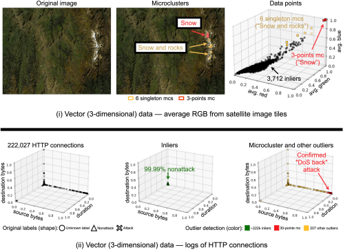
Figure 8: Q4. McCatch is Practical: finding valid mcs unsupervisedly. (i) on a satellite image – it spots a $3$-points mc of snow in a volcano, and other outlying tiles with snow and rocks; (ii) on network security data – it spots a $30$-points mc of confirmed attacks, and other confirmed attacks. (best viewed in color)

Attention routing

We studied the images on the left sides of Figs. 1(i) and 8(i). Each image was split into rectangular tiles from which average RGB values were extracted, thus leading to Shanghai and Volcanoes. Ground truth labels are unknown and, thus, AUROC cannot be computed. Regarding Shanghai, McCatch found two $2$-points clusters formed from unusually colored roofs of buildings (red and blue tiles in Fig. 1(i) – center), and other outlying tiles (in yellow). The red tiles are unusual and alike, and the same happens with the blue ones, while the yellow tiles are unusual but very distinct from one another. The plot in the right side of Fig. 1(i) corroborates our findings; see the red and blue mcs, and the scattered, yellow outliers. Similar results were seen in Volcanoes, with a $3$-points cluster of snow found on the summit of the volcano; see Fig. 8(i). Thus, McCatch can successfully and unsuper-visedly route people’s attention to notable image regions.

Unusual names

Fig. 1(ii) reports results on nondimensional data. We studied Last Names using the L-Edit distance. McCatch earned a $0.75$ AUROC by finding the outliers on the left side of the figure. We investigated these names and discovered that they have a large variety of geographic origins; see the country flags. Distinctly, the low-scored names mostly come from the UK; see the five ones with the lowest scores on the illustration’s right side. We conclude that McCatch distinguished English and NonEnglish names in the data.

Unusual skeletons

Fig. 1(iii) also regards nondimensional data. We studied the $203$ graphs in Skeletons using the Graph edit distance. McCatch earned a perfect AUROC of $1$ by finding all $3$ wild-animal skeletons on the figure’s left side. Thus, it successfully found the unusual, non-human skeletons.

Network attacks

Fig. 8(ii) reports results from HTTP. The raw data is in the left-side plot; there are $222$k connections described by numbers of bytes sent and received, and durations. The inliers and outliers found by McCatch are at the center- and the right-side plots, respectively. AUROC is $0.96$. Note that $99.99\%$ of the inliers are not attacks; the outliers are either confirmed attacks or connections with a clear rarity, as they have oddly large durations, or numbers of bytes sent or received. The most notable result is the detection of a $30$-points mc of confirmed ‘DoS back’ attacks, which are characterized by sending too many bytes to a server aimed at overloading it. Hence, our McCatch unsupervisedly found a cluster of frauds exploiting the same vulnerability in cybersecurity.

V-E Q5. McCatch is ‘Hands-Off’

McCatch needs only a few hyperparameters, namely, $a$, $b$, $c$. It turns out that the values we have used ($15$, $1/10$, $1/10$, respectively), are at a smooth plateau (see Fig. 9): that is, the accuracy is insensitive to the exact choice of hyperparameter values. Specifically, Fig. 9 shows accuracy vs. $a$, $b$, $c$, respectively, and every line corresponds to one of the datasets. Notice that all lines are near flat, highlighting the fact that McCatch needs no hyperparameter fine-tuning. To avoid clutter, we only show the largest real dataset (HTTP) with line-point format.

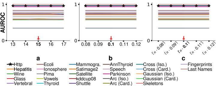
Figure 9: Q5. McCatch is ‘Hands-Off’ and insensitive to the ($a,b,c$) hyper-parameter values: Accuracy has a smooth plateau. (best viewed in color)

VI Conclusions

We presented McCatch to address the microcluster-detection problem. The main idea is to leverage our proposed ‘Oracle’ plot ($1$NN Distance vs. Group $1$NN Distance). McCatch achieves five goals:

1. General Input: McCatch works with any metric dataset, including nondimensional ones, as shown in Fig. 1. It is achieved by depending solely on distances.

2. General Output: McCatch ranks singleton (‘one-off’ outliers) and nonsingleton mcs together, by anomalousness. See Probl. 1 and Def. 7. It is achieved thanks to a new compression-based idea (Fig. 5) to compute scores.

3. Principled: McCatch obeys axioms; see Tab. V. It is achieved thanks to the new group axioms of Fig. 2 and our score-computation strategy that match human intuition.

4. Scalable: McCatch is subquadratic on the number of points, as shown in Lemma 1 and Fig. 7. It is made possible by carefully building on spatial joins and metric trees.

5. ‘Hands-Off’: McCatch needs no manual tuning. It is achieved due to our MDL-based idea to get the Cutoff $d$ from the given data; see Def. 6 and Figs. 4 and 9. We also set hyperparameters to the reasonable defaults of Alg. 1.

No competitor fulfills all of these goals; see Tab. I. Also, McCatch is deterministic, ranks the points, and gives explainable results. We studied $31$ real and synthetic datasets and showed McCatch outperforms $11$ competitors, especially when the data has nonsingleton microclusters or is nondimensional. We also showcased McCatch’s ability to find meaningful mcs in graphs, fingerprints, logs of network connections, text data, and satellite images. For example, it found a $30$-points mc of confirmed attacks in the network logs, taking $\mathit{\sim 3}$ minutes for $222$K points on a stock desktop; see Fig. 8(ii).

Reproducibility: For reproducibility, our data and code are available at https://figshare.com/s/08869576e75b74c6cc55.

References

- [1] C. C. Aggarwal, Outlier Analysis. Springer, 2013.
- [2] G. O. Campos, A. Zimek, J. Sander, R. J. G. B. Campello, B. Micenková, E. Schubert, I. Assent, and M. E. Houle, “On the evaluation of unsupervised outlier detection: measures, datasets, and an empirical study,” DAMI, vol. 30, no. 4, pp. 891–927, Jul. 2016.
- [3] G. H. Orair, C. H. C. Teixeira, W. Meira, Y. Wang, and S. Parthasarathy, “Distance-based outlier detection: Consolidation and renewed bearing,” Proc. VLDB Endow., vol. 3, no. 1–2, p. 1469–1480, sep 2010.
- [4] M.-C. Lee, S. Shekhar, C. Faloutsos, T. N. Hutson, and L. Iasemidis, “Gen2Out: Detecting and ranking generalized anomalies,” in 2021 IEEE International Conference on Big Data (Big Data), 2021, pp. 801–811.
- [5] S. Jiang, R. L. F. Cordeiro, and L. Akoglu, “D.MCA: Outlier detection with explicit micro-cluster assignments,” in Proceedings of the 22nd IEEE International Conference on Data Mining (ICDM), 2022, p. 987–992.
- [6] F. T. Liu, K. M. Ting, and Z.-H. Zhou, “On detecting clustered anomalies using SCiForest,” in Machine Learning and Knowledge Discovery in Databases, 2010, pp. 274–290.
- [7] G. Shabat, D. Segev, and A. Averbuch, “Uncovering unknown unknowns in financial services big data by unsupervised methodologies: Present and future trends,” in Proceedings of the KDD 2017 Workshop on Anomaly Detection in Finance, ADF@KDD 2017, Halifax, Nova Scotia, Canada, August 14, 2017, ser. Proceedings of Machine Learning Research, vol. 71. PMLR, 2017, pp. 8–19.
- [8] Y. Ki and J. W. Yoon, “PD-FDS: purchase density based online credit card fraud detection system,” in Proceedings of the KDD 2017 Workshop on Anomaly Detection in Finance, ADF@KDD 2017, Halifax, Nova Scotia, Canada, August 14, 2017, ser. Proceedings of Machine Learning Research, vol. 71. PMLR, 2017, pp. 76–84.
- [9] A. Jauhri, B. McDanel, and C. Connor, “Outlier detection for large scale manufacturing processes,” in 2015 IEEE International Conference on Big Data (IEEE BigData 2015), Santa Clara, CA, USA, October 29 - November 1, 2015. IEEE Computer Society, 2015, pp. 2771–2774.
- [10] X. Wang, J. Lin, N. Patel, and M. W. Braun, “A self-learning and online algorithm for time series anomaly detection, with application in CPU manufacturing,” in Proceedings of the 25th ACM International Conference on Information and Knowledge Management, CIKM 2016, Indianapolis, IN, USA, October 24-28, 2016. ACM, 2016, pp. 1823–1832.
- [11] S. Kao, A. R. Ganguly, and K. Steinhaeuser, “Motivating complex dependence structures in data mining: A case study with anomaly detection in climate,” in ICDM Workshops 2009, IEEE International Conference on Data Mining Workshops, Miami, Florida, USA, 6 December 2009. IEEE Computer Society, 2009, pp. 223–230.
- [12] M. Das and S. Parthasarathy, “Anomaly detection and spatio-temporal analysis of global climate system,” in Proceedings of the Third International Workshop on Knowledge Discovery from Sensor Data, Paris, France, June 28, 2009. ACM, 2009, pp. 142–150.
- [13] H.-P. Kriegel, M. Schubert, and A. Zimek, “Angle-based outlier detection in high-dimensional data,” in Proceedings of the 14th ACM SIGKDD International Conference on Knowledge Discovery and Data Mining, 2008, p. 444–452.
- [14] S. Papadimitriou, H. Kitagawa, P. Gibbons, and C. Faloutsos, “Loci: fast outlier detection using the local correlation integral,” in Proceedings 19th International Conference on Data Engineering, 2003, pp. 315–326.
- [15] E. M. Knorr and R. T. Ng, “Algorithms for mining distance-based outliers in large datasets,” in Proceedings of the 24rd International Conference on Very Large Data Bases, 1998, p. 392–403.
- [16] C.-H. Chang, J. Yoon, S. O. Arik, M. Udell, and T. Pfister, “Data-efficient and interpretable tabular anomaly detection,” in Proceedings of the 29th ACM SIGKDD Conference on Knowledge Discovery and Data Mining, 2023, p. 190–201.
- [17] R. J. G. B. Campello, D. Moulavi, A. Zimek, and J. Sander, “Hierarchical density estimates for data clustering, visualization, and outlier detection,” ACM Trans. Knowl. Discov. Data, vol. 10, no. 1, 2015.
- [18] F. T. Liu, K. M. Ting, and Z.-H. Zhou, “Isolation-based anomaly detection,” ACM Trans. Knowl. Discov. Data, vol. 6, no. 1, mar 2012.
- [19] S. Ramaswamy, R. Rastogi, and K. Shim, “Efficient algorithms for mining outliers from large data sets,” SIGMOD Rec., vol. 29, no. 2, p. 427–438, 2000.
- [20] K. Zhang, M. Hutter, and H. Jin, “A new local distance-based outlier detection approach for scattered real-world data,” in Advances in Knowledge Discovery and Data Mining, T. Theeramunkong, B. Kijsirikul, N. Cercone, and T.-B. Ho, Eds. Berlin, Heidelberg: Springer Berlin Heidelberg, 2009, pp. 813–822.
- [21] M. M. Breunig, H.-P. Kriegel, R. T. Ng, and J. Sander, “Lof: Identifying density-based local outliers,” in Proceedings of the 2000 ACM SIGMOD International Conference on Management of Data, 2000, p. 93–104.
- [22] V. Hautamaki, I. Karkkainen, and P. Franti, “Outlier detection using k-nearest neighbour graph,” in Proceedings of the 17th International Conference on Pattern Recognition, 2004, pp. 430–433.
- [23] R. Pamula, J. K. Deka, and S. Nandi, “An outlier detection method based on clustering,” in 2011 Second International Conference on Emerging Applications of Information Technology, 2011, pp. 253–256.
- [24] S. Zhang, V. Ursekar, and L. Akoglu, “Sparx: Distributed outlier detection at scale,” in Proceedings of the 28th ACM SIGKDD Conference on Knowledge Discovery and Data Mining, 2022, p. 4530–4540.
- [25] L. Kong, A. Huet, D. Rossi, and M. Sozio, “Tree-based kendall’s maximization for explainable unsupervised anomaly detection,” in 2023 IEEE International Conference on Data Mining (ICDM), 2023, pp. 1073–1078.
- [26] L. Ruff, N. Görnitz, L. Deecke, S. A. Siddiqui, R. A. Vandermeulen, A. Binder, E. Müller, and M. Kloft, “Deep one-class classification,” in Proceedings of the 35th International Conference on Machine Learning, 2018, pp. 4390–4399.
- [27] H. Xiang, X. Zhang, M. Dras, A. Beheshti, W. Dou, and X. Xu, “Deep optimal isolation forest with genetic algorithm for anomaly detection,” in 2023 IEEE International Conference on Data Mining (ICDM), 2023, pp. 678–687.
- [28] C. Zhou and R. C. Paffenroth, “Anomaly detection with robust deep autoencoders,” in Proceedings of the 23rd ACM SIGKDD International Conference on Knowledge Discovery and Data Mining, 2017, p. 665–674.
- [29] M. Ester, H.-P. Kriegel, J. Sander, and X. Xu, “A Density-Based Algorithm for Discovering Clusters in Large Spatial Databases with Noise,” in International Conference on Knowledge Discovery and Data Mining, USA, Oregon, Portland, 1996, pp. 226–231.
- [30] S. Chawla and A. Gionis, “k-means–: A unified approach to clustering and outlier detection,” in Proceedings of the 13th SIAM International Conference on Data Mining (SDM), 2013, pp. 189–197.
- [31] M. Ankerst, M. M. Breunig, H.-P. Kriegel, and J. Sander, “Optics: Ordering points to identify the clustering structure,” ACM Sigmod record, vol. 28, no. 2, pp. 49–60, 1999.
- [32] I. Borg and P. Groenen, Modern Multidimensional Scaling: theory and applications, 2nd ed. Springer-Verlag, 2005.
- [33] L. McInnes, J. Healy, and J. Melville, “Umap: Uniform manifold approximation and projection for dimension reduction,” 2020.
- [34] L. van der Maaten and G. Hinton, “Visualizing data using t-sne,” Journal of Machine Learning Research, vol. 9, no. 86, pp. 2579–2605, 2008. [Online]. Available: http://jmlr.org/papers/v9/vandermaaten08a.html
- [35] C. T. Jr., A. J. M. Traina, C. Faloutsos, and B. Seeger, “Fast indexing and visualization of metric data sets using slim-trees,” IEEE Trans. Knowl. Data Eng., vol. 14, no. 2, pp. 244–260, 2002.
- [36] P. Ciaccia, M. Patella, and P. Zezula, “M-tree: An efficient access method for similarity search in metric spaces,” in Proceedings of the 23rd International Conference on Very Large Data Bases, ser. VLDB ’97. San Francisco, CA, USA: Morgan Kaufmann Publishers Inc., 1997, p. 426–435.
- [37] P. Grünwald, “A tutorial introduction to the minimum description length principle,” 2004.
- [38] J. Rissanen, “A universal prior for integers and estimation by minimum description length,” The Annals of Statistics, vol. 11, no. 2, pp. 416–431, 6 1983.
- [39] D. Chakrabarti, S. Papadimitriou, D. S. Modha, and C. Faloutsos, “Fully automatic cross-associations,” in KDD. ACM, 2004, pp. 79–88.
- [40] C. Faloutsos and I. Kamel, “Beyond uniformity and independence: Analysis of r-trees using the concept of fractal dimension,” in PODS. ACM Press, 1994, pp. 4–13.
- [41] B. Pagel, F. Korn, and C. Faloutsos, “Deflating the dimensionality curse using multiple fractal dimensions,” in ICDE. IEEE Computer Society, 2000, pp. 589–598.
- [42] C. T. Jr., A. J. M. Traina, L. Wu, and C. Faloutsos, “Fast feature selection using fractal dimension,” in SBBD. CEFET-PB, 2000, pp. 158–171.
- [43] B. Bryan, F. Eberhardt, and C. Faloutsos, “Compact similarity joins,” in ICDE. IEEE Computer Society, 2008, pp. 346–355.
- [44] T. R. Bandaragoda, K. M. Ting, D. Albrecht, F. T. Liu, Y. Zhu, and J. R. Wells, “Isolation-based anomaly detection using nearest-neighbor ensembles,” Computational Intelligence, vol. 34, no. 4, pp. 968–998, 2018. [Online]. Available: https://onlinelibrary.wiley.com/doi/abs/10.1111/coin.12156
- [45] K. M. Ting, B. Xu, T. Washio, and Z. Zhou, “Isolation distributional kernel: A new tool for kernel based anomaly detection,” in KDD ’20: The 26th ACM SIGKDD Conference on Knowledge Discovery and Data Mining, Virtual Event, CA, USA, August 23-27, 2020, R. Gupta, Y. Liu, J. Tang, and B. A. Prakash, Eds. ACM, 2020, pp. 198–206. [Online]. Available: https://doi.org/10.1145/3394486.3403062
- [46] The PostgreSQL Global Development Group, “PostgreSQL Documentation: F.17. fuzzystrmatch - determine string similarities and distance,” https://www.postgresql.org/docs/current/fuzzystrmatch.html, Accessed: 2024-02-21.
- [47] L. Vincent, “Graphs and mathematical morphology,” Signal Processing, vol. 16, no. 4, pp. 365–388, 1989. [Online]. Available: https://doi.org/10.1016/0165-1684(89)90031-5
- [48] M. Pawlik and N. Augsten, “Efficient computation of the tree edit distance,” ACM Trans. Database Syst., vol. 40, no. 1, mar 2015. [Online]. Available: https://doi.org/10.1145/2699485