Top anomalous chromomagnetic dipole moment in the Bestest Little Higgs Model

Abstract

We investigate the anomalous Chromomagnetic Dipole Moment (CMDM), $\hat{\mu}_{t}^{BLHM}$, of the top quark in the Bestest Little Higgs Model (BLHM). We include new interactions with the involvement of the extended CKM matrix of the BLHM and we explore most of the allowed parameter space, obtaining multiple CMDM in the range of $10^{-4}-10^{-2}$. We consider experimental and model parameter uncertainties to integrate them into all our calculations using a Monte Carlo method. This enables us to determine the extent to which deviations arising from experimental errors can be accommodated within the statistical errors of the model and which relate to the physics framework of the BLHM, guiding future theory, phenomenological, and experimental research.

I INTRODUCTION

The search for new physics in extensions of the Standard Model (SM) leverages various perspectives shared among different theories, such as the extended Higgs mechanism, extra dimensions, and symmetries giving rise to new fields. In this context, we take advantage of the exceptional properties of the top quark to explore its CMDM in the BLHM [1] and update its magnitude [2] by including contributions arising from the new interactions introduced in the article [3] with flavor-changing mediated by two extended matrices $V_{Hu}$ and $V_{Hd}$ of the type $V_{CKM}$ (Cabibbo-Kobayashi-Maskawa) [4]. The Chromoelectric Dipole Moment (CEDM) is identically zero at one loop in the BLHM as it was proved in [2], so we will not address details regarding it in this study. The CMDM of the top quark has been analyzed in various relevant studies both in the SM and in other extensions [5, 6, 7, 8, 9]. The interest lies in the massive nature of the top quark and its connection to heavy particles proposed in Extended Standard Model (ESM) frameworks. In this context, the theoretical framework provided by the BLHM and the type I Two Higgs Doublets Model (2HDM) offers an enriched perspective within the broader landscape of Little Higgs Models (LHM). It concisely and naturally addresses issues such as custodial symmetry violation, divergent singlets, the mass ratio of extended bosons and quarks, among others [1]. A unique aspect of this model is its modular structure, which requires two distinct breaking scales, $f$ and $F$, with the condition $F>f$. In this way, the heavy quarks depend on the scale $f$, and the heavy gauge bosons depend on both $f$ and $F$, where $F$ can be as large as necessary. Despite the advantages and solutions offered by the BLHM, it has not been explored as extensively as other models within the LHM family, mainly due to the experimental challenges associated with generating increasingly higher masses. However, several investigations have been conducted in the BLHM in the area of dipoles [2, 10, 11, 12] and rare top decays [3].

Currently, the measurement of the CMDM given by the CMS Collaboration at the LHC [13] using $pp$ collisions at $13$ TeV and with an integrated luminosity of $35.9$ fb^-1 is

$$\hat{\mu}^{Exp}_{t}=-0.024^{+0.013}_{-0.009}(\mathrm{stat})^{+0.016}_{-0.011}(\mathrm{syst}).$$ (1)

In the context of ESM frameworks, we can find a preliminary calculation of the CMDM in [14, 15, 5]. In the case of 2HDM models, the calculation of the CMDM has been performed in the Littlest Higgs with T symmetry (LHT) [6] with an estimate of $10^{-3}-10^{-4}$ and in four generations of fermions [16] with the result $10^{-1}-10^{-2}$. The first calculation of the CMDM in the BLHM was carried out in [2], with an estimated value of $\hat{\mu}^{BLHM}_{t}\sim 10^{-4}-10^{-6}$. The previous result was obtained for $\beta=1.35$ radians in the BLHM, where $tan\beta=v_{1}/v_{2}$ and $v^{2}_{SM}=v_{1}^{2}+v_{2}^{2}$. In our case, we have calculated the $\hat{\mu}_{t}^{BLHM}$ for each angle $\beta$ in the range $0.15\leq\beta\leq 1.49$ with results $10^{-4}\leq\hat{\mu}_{t}^{BLHM}\leq 10^{-2}$.

This paper is structured as follows: In Section II, we provide a brief review of the BLHM in order to establish the physics framework employed in our calculations. In Section III, we describe the sector of the BLHM that includes $gt\bar{t}$ vertex needed for the $\hat{\mu}^{BLHM}$ calculation. Section IV, discusses the allowed phase space within the calculations of the CMDM. In Section V, we detail the various scenarios in which we calculate the CMDM and describe our error propagation methodology. Section VI, contains a summary of our results. Finally, we give our conclusions in Section VII. In Appendix A, we provide the necessary Feynman rules to calculate the CMDM. In Appendix B, we provide detailed plots of our calculations in order to display the confidence intervals, which can help in guiding future research.

II Brief review of the BLHM

The BLHM [1] originates from a symmetry group $SO(6)_{A}\times SO(6)_{B}$, which breaks at the scale $f$ towards $SO(6)_{V}$ when the non-linear sigma field $\Sigma$ acquires a vacuum expectation value (VEV), denoted as $\langle\Sigma\rangle=1$. This leads to the emergence of 15 pseudo-Nambu Goldstone bosons, parameterized by the electroweak triplet $\phi^{a}$ with zero hypercharges $(a=1,2,3)$ and the triplet $\eta^{a}$, where $(\eta_{1},\eta_{2})$ form a complex singlet with hypercharge, and $\eta_{3}$ is a real singlet,

$$\Sigma=e^{i\Pi/f}e^{2i\Pi_{h}/f}e^{i\Pi/f},$$ (2)

$$\Pi=\begin{pmatrix}\phi_{a}T^{a}_{L}+\eta_{a}T^{a}_{R}&0&0\\ 0&0&i\sigma/\sqrt{2}\\ 0&-i\sigma/\sqrt{2}&0\end{pmatrix},$$ (3)

$$\Pi_{h}=\begin{pmatrix}0_{4\times 4}&h_{1}&h_{2}\\ -h^{T}_{1}&0&0\\ -h^{T}_{2}&0&0\end{pmatrix},$$ (4)

where $h_{i}^{T}=(h_{i1},h_{i2},h_{i3},h_{i4})$, $(i=1,2)$, represent Higgs quadruplets of $SO(4)$. The scalar field $\sigma$ is required to generate a collective quartic coupling [1]. $T_{L,R}^{a}$ denote the generators of $SU(2)_{L}$ and $SU(2)_{R}$.

II.1 Scalar sector

In the BLHM, two operators are required to generate the quartic coupling of the Higgs through collective symmetry breaking; none of these operators alone allows the Higgs to acquire a potential:

$$P_{5}=diag(0,0,0,0,1,0),$$ (5)

$$P_{6}=diag(0,0,0,0,0,1).$$

In this way, we can write the quartic potential as [1]

$$V_{q} = \frac{1}{4}\lambda_{65}f^{4}Tr(P_{6}\Sigma P_{5}\Sigma^{T})$$

$$+ \frac{1}{4}\lambda_{56}f^{4}Tr(P_{5}\Sigma P_{6}\Sigma^{T})$$

$$= \frac{1}{4}\lambda_{65}f^{4}(\Sigma_{65})^{2}+\frac{1}{4}\lambda_{56}f^{4}(\Sigma_{56})^{2},$$

where $\lambda_{56}$ and $\lambda_{65}$ are coefficients that must be nonzero to achieve collective symmetry breaking and generate a Higgs quartic coupling. The first part of Eq. (II.1) breaks $SO(6)_{A}\times SO(6)_{B}\to SO(5)_{A5}\times SO(5)_{B6}$, with $SO(5)_{A5}$ preventing $h_{1}$ from acquiring a potential and $SO(5)_{B6}$ doing the same for $h_{2}$. The second part of Eq. (II.1) breaks $SO(6)_{A}\times SO(6)_{B}\to SO(5)_{A6}\times SO(5)_{B5}$. If we expand Eq. (2) in powers of $1/f$ and substitute it into Eq. (II.1), we obtain

$$V_{q}=\frac{\lambda_{65}}{2}\left(f\sigma-\frac{1}{\sqrt{2}}h_{1}^{T}h_{2}+\dots\right)^{2}$$ (7)

$$+\frac{\lambda_{56}}{2}\left(f\sigma+\frac{1}{\sqrt{2}}h_{1}^{T}h_{2}+\dots\right)^{2}.$$

This potential generates a mass for $\sigma$,

$$m_{\sigma}^{2}=(\lambda_{65}+\lambda_{56})f^{2}.$$ (8)

From Eq. (7), each term alone seems to generate a quartic coupling for the Higgses, this can be eliminated by a redefinition of the field $\sigma\to\pm\frac{h^{T}_{1}h_{2}}{\sqrt{2}f}$, where the upper and lower signs of this transformation correspond to the first and second operators in Eq. (7), respectively. Collectively, though, the two terms in Eq. (7) produce a tree-level quartic Higgs; this occurs after integrating $\sigma$ [1, 17, 18]:

$$V_{q}=\frac{\lambda_{56}\lambda_{65}}{\lambda_{56}+\lambda_{65}}\left(h_{1}^{T}h_{2}\right)^{2}=\frac{1}{2}\lambda_{0}\left(h_{1}^{T}h_{2}\right)^{2}.$$ (9)

The expression obtained has the desired form of a collective quartic potential [1, 17].

In this way, we obtain the form of a quartic collective potential proportional to two different couplings [1]. We can observe that $\lambda_{0}$ will be zero if $\lambda_{56}$, $\lambda_{65}$, or both are zero. This illustrates the principle of collective symmetry breaking.

If we exclude gauge interactions, not all scalars gain mass, and therefore, we need to introduce the potential,

$$V_{s} = -\frac{f^{2}}{4}m_{4}^{2}Tr\left(\Delta^{\dagger}M_{26}\Sigma M^{\dagger}_{26}+\Delta M_{26}\Sigma^{\dagger}M^{\dagger}_{26}\right)$$ (10)

$$-\frac{f^{2}}{4}\left(m_{5}^{2}\Sigma_{55}+m_{6}^{2}\Sigma_{66}\right),$$

where $m_{4}$, $m_{5}$, and $m_{6}$ are mass parameters, and $(\Sigma_{55},\Sigma_{66})$ are matrix elements of Eq. (2). Here, $M_{26}$ is a matrix that contracts the $SU(2)$ indices of $\Delta$ with the $SO(6)$ indices of $\Sigma$,

$$M_{26}=\frac{1}{\sqrt{2}}\begin{pmatrix}0&0&1&i&0&0\\ 1&-i&0&0&0&0\end{pmatrix}.$$ (11)

The $\Delta$ operator arises from a global symmetry $SU(2)_{C}\times SU(2)_{D}$ that is broken to a diagonal $SU(2)$ at the scale $F>f$ when it develops a VEV, $\langle\Delta\rangle=1$. We can parameterize it in the form

$$\Delta=e^{2i\Pi_{d}/F},\hskip 8.5359pt\Pi_{d}=\chi_{a}\frac{\tau_{a}}{2}\hskip 8.5359pt(a=1,2,3),$$ (12)

where the matrix $\Pi_{d}$ contains the scalars of the triplet $\chi_{a}$ that mix with the triplet $\phi_{a}$, and $\tau_{a}$ represents the Pauli matrices. $\Delta$ is connected to $\Sigma$ in such a way that the diagonal subgroup of $SU(2)_{A}\times SU(2)_{B}\subset SO(6)_{A}\times SO(6)_{B}$ is identified as the SM $SU(2)_{L}$ group. If we expand the operator $\Delta$ in powers of $1/F$ and substitute it into Eq. (10), we obtain

$$V_{s}=\frac{1}{2}\left(m^{2}_{\phi}\phi^{2}_{a}+m^{2}_{\eta}\eta^{2}_{a}+m^{2}_{1}h^{T}_{1}h_{1}+m^{2}_{2}h^{T}_{2}h_{2}\right),$$ (13)

where

$$m^{2}_{\phi} = m^{2}_{\eta}=m^{2}_{4},$$ (14)

$$m^{2}_{1} = \frac{1}{2}(m^{2}_{4}+m^{2}_{5}),$$

$$m^{2}_{2} = \frac{1}{2}(m^{2}_{4}+m^{2}_{6}).$$

To trigger EWSB, the next potential term is introduced[1]:

$$V_{B_{\mu}}=m_{56}^{2}f^{2}\Sigma_{56}+m_{65}^{2}f^{2}\Sigma_{65},$$ (15)

where the mass terms $m_{56}$ and $m_{65}$ correspond to the matrix elements $\Sigma_{56}$ and $\Sigma_{65}$, respectively. Finally, we have the complete scalar potential,

$$V=V_{q}+V_{s}+V_{B_{\mu}}.$$ (16)

We need a potential for the Higgs doublets; therefore, we minimize Eq. (16) concerning $\sigma$ and substitute the result back into Eq. (16), obtaining the expression:

$$V_{H} = \frac{1}{2}\Big{[}m_{1}^{2}h_{1}^{T}h_{1}+m_{2}^{2}h_{2}^{T}h_{2}-2B_{\mu}h_{1}^{T}h_{2}$$ (17)

$$+ \lambda_{0}(h_{1}^{T}h_{2})^{2}\Big{]},$$

where

$$B_{\mu}=2\frac{\lambda_{56}m_{65}^{2}+\lambda_{65}m_{56}^{2}}{\lambda_{56}+\lambda_{65}}.$$ (18)

The potential (17) has a minimum when $m_{1}m_{2}>0$, and EWSB requires that $B_{\mu}>m_{1}m_{2}$. Here, we can observe that the term $B_{\mu}$ disappears if $\lambda_{56}=0$ or $\lambda_{65}=0$ or both are zero in Eq. (18). After EWSB, Higgs doublets acquire VEVs given by

$$\langle h_{1}\rangle=v_{1},\hskip 8.5359pt\langle h_{2}\rangle=v_{2}.$$ (19)

The two terms in (19) must minimize Eq. (17), resulting in the following relationships

$$v_{1}^{2}=\frac{1}{\lambda_{0}}\frac{m_{2}}{m_{1}}(B_{\mu}-m_{1}m_{2}),$$ (20)

$$v_{2}^{2}=\frac{1}{\lambda_{0}}\frac{m_{1}}{m_{2}}(B_{\mu}-m_{1}m_{2}),$$ (21)

and it is defined the $\beta$ angle between $v_{1}$ and $v_{2}$ [1], such that,

$$\tan\beta=\frac{\langle h_{11}\rangle}{\langle h_{21}\rangle}=\frac{v_{1}}{v_{2}}=\frac{m_{2}}{m_{1}},$$ (22)

in this way, we have

$$v^{2} = v_{1}^{2}+v_{2}^{2}$$

$$= \frac{1}{\lambda_{0}}\left(\frac{m_{1}^{2}+m_{2}^{2}}{m_{1}m_{2}}\right)(B_{\mu}-m_{1}m_{2})$$

$$\simeq (246\;GeV)^{2}.$$

After the EWSB, the scalar sector [1, 18] produces massive states of $h^{0}$ (SM Higgs), $A^{0}$, $H^{\pm}$ and $H^{0}$ with masses

$$m^{2}_{G^{0}}=m^{2}_{G^{\pm}}=0,$$ (26)

$$m^{2}_{A^{0}}=m^{2}_{H^{\pm}}=m^{2}_{1}+m^{2}_{2},$$

$$m^{2}_{H^{0}}=\frac{B_{\mu}}{\sin 2\beta}$$

$$+ \sqrt{\frac{B^{2}_{\mu}}{\sin^{2}2\beta}-2\lambda_{0}\beta_{\mu}v^{2}\sin 2\beta+\lambda_{0}^{2}v^{4}\sin^{2}2\beta},$$

where $G^{0}$ and $G^{\pm}$ are Goldstone bosons that are eaten to give masses to the $W^{\pm},Z$ bosons of the SM.

II.2 Gauge boson sector

The gauge kinetic terms are given by the Lagrangian [1, 18]

$$\mathcal{L}=\frac{f^{2}}{8}Tr\left(D_{\mu}\Sigma^{{\dagger}}D^{\mu}\Sigma\right)+\frac{F^{2}}{4}Tr\left(D_{\mu}\Delta^{{\dagger}}D^{\mu}\Delta\right),$$ (27)

where $D_{\mu}\Sigma$ and $D_{\mu}\Delta$ are covariant derivatives,

$$D_{\mu}\Sigma = i\sum_{a}\left(g_{A}A_{1\mu}^{a}T_{L}^{a}\Sigma-g_{B}A_{2\mu}^{a}\Sigma T^{a}_{L}\right)$$

$$+ ig^{\prime}B_{3}\left(T^{3}_{R}\Sigma-\Sigma T^{3}_{R}\right),$$

$$D_{\mu}\Delta = \frac{i}{2}\sum_{a}\left(g_{A}A^{a}_{1\mu}\tau_{a}\Delta-g_{B}A^{a}_{2\mu}\Delta\tau_{a}\right),$$ (29)

while $(A^{a}_{1\mu},A^{a}_{2\mu})$ are gauge boson eigenstates, $g^{\prime}$ is the coupling of $U(1)_{Y}$, and $g$ is the coupling of the $SU(2)_{L}$. They are related to $SU(2)_{A}\times SU(2)_{B}$ couplings $g_{A}$ and $g_{B}$ in the following way

$$g=\frac{g_{A}g_{B}}{\sqrt{g_{A}^{2}+g_{B}^{2}}},$$ (30)

$$s_{g}=\sin\theta_{g}=\frac{g_{A}}{\sqrt{g_{A}^{2}+g_{B}^{2}}},$$ (31)

$$c_{g}=\cos\theta_{g}=\frac{g_{B}}{\sqrt{g_{A}^{2}+g_{B}^{2}}},$$ (32)

here, $\theta_{g}$ is the mixing angle, and if $g_{A}=g_{B}$, then $\tan\theta_{g}=1$.

In the BLHM, both the masses of the heavy gauge bosons $W^{\prime\pm}$, $Z^{\prime}$ and those of the SM bosons are also generated [1, 18],

$$m_{Z^{\prime}}^{2} = \frac{1}{4}(g_{A}^{2}+g_{B}^{2})(f^{2}+F^{2})-\frac{1}{4}g^{2}v^{2}$$

$$+ \Bigg{(}2g^{2}+\frac{3f^{2}}{f^{2}+F^{2}}$$

$$\times (g^{2}+g^{\prime}\,{}^{2})(s_{g}^{2}-c_{g}^{2})\Bigg{)}\frac{v^{4}}{48f^{2}},$$

$$m_{W^{\prime}}^{2} = \frac{1}{4}(g_{A}^{2}+g_{B}^{2})(f^{2}+F^{2})-m_{W}^{2}.$$ (34)

II.3 Fermion sector

The fermion sector of the BLHM is governed by the Lagrangian [1]

$$\mathcal{L}_{t} = y_{1}fQ^{T}S\,\Sigma\,SU^{c}+y_{2}fQ_{a}^{\prime T}\Sigma\,U^{c}$$

$$+ y_{3}fQ^{T}\Sigma\,U_{5}^{\prime c}+y_{b}fq_{3}^{T}(-2iT_{R}^{3}\Sigma)U_{b}^{c}+\textrm{h.c.},$$

where $(Q,Q^{\prime})$ and $(U,U^{\prime})$ are multiplets of $SO(6)_{A}$ and $SO(6)_{B}$, respectively, given by:

$$Q^{T} = \frac{1}{\sqrt{2}}\Big{[}-(Q_{a1}+Q_{b2}),i(Q_{a1}-Q_{b2}),$$

$$(Q_{a2}-Q_{b1}),i(Q_{a2}+Q_{b1}),Q_{5},Q_{6}\Big{]},$$

where $(Q_{a1},Q_{a2})$ and $(Q_{b1},Q_{b2})$ are $SU(2)_{L}$ doublets. $(Q_{5},Q_{6})$ are singlets under $SU(2)_{L}\times SU(2)_{R}=SO(4)$. While

$$(U^{c})^{T} = \frac{1}{\sqrt{2}}\Big{[}-(U^{c}_{b1}+U^{c}_{a2}),i(U^{c}_{b1}-U^{c}_{a2}),$$

$$(U^{c}_{b2}-U^{c}_{a1}),i(U^{c}_{b2}+U^{c}_{a1}),U^{c}_{5},U^{c}_{6}\Big{]},$$

where $(U^{c}_{a2},-U^{c}_{a1})$ and $(-U^{c}_{b2},U^{c}_{b1})$ are doublets of $SU(2)_{L}$ along with the singlets $(U_{5},U_{6})$. And

$$Q^{\prime T}_{a} = \frac{1}{\sqrt{2}}\left(-Q^{\prime}_{a1},iQ^{\prime}_{a1},Q^{\prime}_{a2},iQ^{\prime}_{a2},0,0\right)$$ (38)

$$U^{\prime cT}_{5} = (0,0,0,0,U^{\prime c}_{5},0),$$ (39)

are a doublet of $SU(2)_{A}$ and a singlet of $SU(2)_{A,B}$, respectively. $S=diag(1,1,1,1,-1,-1)$ is a symmetry operator, $(y_{1},y_{2},y_{3})$ represent Yukawa couplings, and the term $(q_{3},U_{b}^{c})$ in Eq. (II.3) contains information about the bottom quark. The BLHM implements new physics in the gauge, fermion, and Higgs sectors, which implies the existence of partner particles for most SM particles. Since top quark loops provide the most significant divergent quantum corrections to the Higgs mass in the SM, the new heavy quarks, in the BLHM scenario, will be crucial for solving the hierarchy problem. Those heavy quarks are: $T$, $T^{5}$, $T^{6}$, $T^{2/3}$, $T^{5/3}$, and $B$, all of which have associated masses [1]:

$$m_{T}^{2} = (y_{1}^{2}+y_{2}^{2})f^{2}$$

$$+ \frac{9v_{1}^{2}y_{1}^{2}y_{2}^{2}y_{3}^{2}}{(y_{1}^{2}+y_{2}^{2})(y_{2}^{2}-y_{3}^{2})},$$

$$m_{T^{5}}^{2} = (y_{1}^{2}+y_{3}^{2})f^{2}$$

$$- \frac{9v_{1}^{2}y_{1}^{2}y_{2}^{2}y_{3}^{2}}{(y_{1}^{2}+y_{3}^{2})(y_{2}^{2}-y_{3}^{2})},$$

$$m_{T^{6}}^{2} = m_{T^{2/3}}^{2}=m_{T^{5/3}}^{2}=y_{1}^{2}f^{2},$$ (42)

$$m_{B}^{2} = y_{B}^{2}f^{2}=(y_{1}^{2}+y_{2}^{2})f^{2}.$$ (43)

In the quark sector Lagrangian [1], the Yukawa couplings must satisfy $0<y_{i}<1$. The masses of $t$ and $b$ are also generated by the Yukawa couplings $y_{t}$ and $y_{b}$ [18]

$$m^{2}_{t} = y_{t}^{2}v_{1}^{2},$$ (44)

$$m^{2}_{b} = y_{b}^{2}v_{1}^{2}-\frac{2y^{2}_{b}}{3\sin^{2}\beta}\frac{v^{4}_{1}}{f^{2}}.$$ (45)

The coupling $y_{t}$,

$$y_{t}^{2}=\frac{9y_{1}^{2}y_{2}^{2}y_{3}^{2}}{(y_{1}^{2}+y_{2}^{2})(y_{1}^{2}+y_{3}^{2})},$$ (46)

is part of the measure of fine-tuning in the BLHM [18],

$$\Psi=\frac{27f^{2}}{8\pi^{2}v^{2}\lambda_{0}\cos^{2}\beta}\frac{|y_{1}|^{2}|y_{2}|^{2}|y_{3}|^{2}}{|y_{2}|^{2}-|y_{3}|^{2}}\log\frac{|y_{1}|^{2}+|y_{2}|^{2}}{|y_{1}|^{2}+|y_{3}|^{2}}.$$ (47)

II.4 Flavor mixing in the BLHM

We have adopted the flavor structure scheme proposed in [3] for the BLHM, as it increases the number of interactions without affecting the fundamental symmetries of the model or altering the coupling vertices of heavy top-type quarks with SM quarks. The modification made by the authors in [3] consists of increasing the terms in the BLHM Lagrangians that involve interactions between the fields $(H^{\pm},\phi^{\pm},\eta^{\pm})$, the heavy quark $B$ and the light SM quarks $(u,c,d,s)$. In this way, for scalar interactions, the terms

$$y_{B}fq_{1}(-2iT_{R}^{2}\Sigma)d_{B}^{c},\hskip 5.69046pty_{B}fq_{2}(-2iT_{R}^{2}\Sigma)d_{B}^{c},$$ (48)

are added to the Lagrangian II.3. Where $y_{B}^{2}=y_{1}^{2}+y_{2}^{2}$ is the Yukawa coupling of heavy $B$ quark, $q_{1}$ and $q_{2}$ are multiplets of light SM quarks and $d_{B}^{c}$ is a new multiplet containing the heavy $B$ quark. As for the vectorial interactions among the fields $W^{\pm},W^{\prime\pm}$, the heavy quark $B$, and the light SM quarks, terms

$$\sum_{i=1}^{2}i\bar{\sigma}_{\mu}Q^{\dagger}_{3}D^{\mu}q_{i},\hskip 14.22636pt\sum_{i=1}^{4}i\bar{\sigma}_{\mu}q_{i}^{\prime\dagger}D^{\mu}U^{c}$$ (49)

are added to the Lagrangian that describes fermion-gauge interactions [1, 18] in the BLHM. In this case, the multiplet $Q_{3}$ contains the heavy quark $B$, and the multiplets $q^{\prime}_{i}$ represents the light quarks $(u,c,d,s)$. These contributions made to the BLHM in [3] extend the phenomenology provided by the model in such a way that two CKM-like unitary matrices, $V_{Hu}$ and $V_{Hd}$, can now be associated, satisfying the relation $V_{CKM}=V_{Hu}^{\dagger}V_{Hd}$, where $V_{CKM}$ is the Cabibbo-Kobayashi-Maskawa matrix [4].

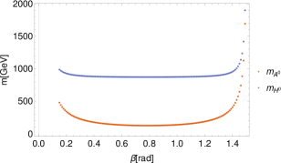
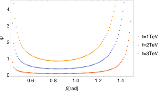
Figure 1: In the left plot, the variation of the masses $m_{A^{0}}$ and $m_{H^{0}}$ with respect to the angle $\beta$ is depicted. The right plot illustrates the variation of the fine-tuning parameter $\Psi$ against the angle $\beta$ for $f=(1,2,3)$ TeV.

III The chromomagnetic dipole moment in the BLHM

The description of the contributions of the vertex $g\bar{t}t$ is given by the effective Lagrangian:

$$\mathcal{L}_{eff}=-\frac{1}{2}\bar{t}\sigma^{\mu\nu}\left(\hat{\mu}_{t}+i\hat{d}_{t}\gamma^{5}\right)tG^{a}_{\mu\nu}T^{a},$$ (50)

where $G^{a}_{\mu\nu}$ is the gluon strength tensor, $T^{a}$ are the $SU(3)$ generators, $\hat{\mu}_{t}$ is the CMDM and $\hat{d}_{t}$ is the CEDM such that

$$\hat{\mu}_{t}=\frac{m_{t}}{g_{s}}\mu_{t},\hskip 14.22636pt\hat{d}_{t}=\frac{m_{t}}{g_{s}}d_{t}.$$ (51)

The definitions given for Eq. (51) are the standard relations for the CMDM and the CEDM in the literature on the subject because $\mathcal{L}_{eff}$ has dimension 5, where $m_{t}$ is the mass of the top quark and $g_{s}=\sqrt{4\pi\alpha_{s}}$ is the coupling constant of the group. In our case, we only need to calculate the chromomagnetic form factor $\mu_{t}$ from the one-loop contributions of the scalar fields $A^{0},H^{0},H^{\pm},h^{0},\sigma,\phi^{0},\phi^{\pm},\eta^{0},\eta^{\pm}$, the vector fields $Z^{0},Z^{\prime},W^{\pm},W^{\prime\pm}$, and the heavy quarks $T,T^{5},T^{6},T^{2/3},T^{5/3},B$.

IV Parameter space of the BLHM

Since its publication, the BLHM has been assessed over different parameter spaces that are convenient according to the experimental data available at the respective times. Developed before the discovery of the Higgs boson, Schmaltz, et al. [1], considered the model for a Higgs mass between $115$ GeV and $250$ GeV. In the subsequent publications [18, 19, 20, 21], the Yukawa couplings $(y_{1},y_{2},y_{3})$ are parameterized using the same method, and $m_{h^{0}}$ is kept around 125 GeV. In [2, 3], the authors use a different parameter space with the aim of optimizing and constraining the BLHM according to the new experimental data. In this way, in this study, we also use the same parameter space based on the variation of the mixing angle $\beta$ between the vacuum expectation values $v_{1},v_{2}$ such that $\tan\beta=v_{1}/v_{2}$. In this implementation, the Yukawa couplings of the BLHM are maintained in the range $0<y_{i}<1$, ensuring that the relation 46 is satisfied under the condition 44 and the value $m_{t}=172.13$ GeV [22]. We solve Eq.(26) to deduce the masses of the scalar bosons in the model considering $0.15\leq\beta\leq 1.49$ radians and $m_{h^{0}}=125.46$ GeV [23] under the condition $\lambda^{0}<4\pi$ [21]. It is also necessary to determine the mixing angle $\alpha$ between $h^{0}$ and $H^{0}$ through the relation [18]

$$\tan\alpha=\frac{1}{B_{\mu}-\lambda_{0}v^{2}\sin 2\beta}\Bigg{(}B_{\mu}\cot 2\beta$$

$$+ \sqrt{\frac{B_{\mu}^{2}}{\sin^{2}2\beta}-2\lambda_{0}B_{\mu}v^{2}\sin 2\beta+\lambda_{0}^{2}v^{4}\sin^{2}2\beta}\Bigg{)}.$$

The ranges for parameters and masses of the heavy scalar bosons are shown in Table 1.

Table 1: Parameters and scalar masses of the BLHM.

Parameter	Values
	Min	Max	Unit
$\beta$	0.15	1.49	rad
$\alpha$	-0.25	1.08	rad
$y_{3}$	0.32	0.96	–
$m_{A^{0}}$	125.00	1693.04	GeV
$m_{H^{0}}$	872.04	1900.3	GeV
$m_{H^{\pm}}$	125.00	1693.04	GeV

Table 2: Parameters and scalar masses constrained in the BLHM.

Parameter	$f(1\,{\scriptstyle\text{TeV}})$		$f(2\,{\scriptstyle\text{TeV}})$		$f(3\,{\scriptstyle\text{TeV}})$
	Min	Max	Min	Max	Min	Max	Unit
$\beta$	0.79	1.47	0.79	1.36	0.79	1.24	rad
$\alpha$	0.38	1.06	0.38	0.95	0.38	0.83	rad
$\Psi$	0.096	2.11	0.38	2.03	0.87	2.04	–
$m_{A^{0}}$	125.0	884.86	125.0	322.75	125.0	207.07	GeV
$m_{H^{0}}$	872.04	1236.06	872.04	921.42	872.04	887.53	GeV
$m_{H^{\pm}}$	125.0	884.86	125.0	322.75	125.0	207.07	GeV

Due to the structure of the Yukawa couplings in the BLHM, the authors [1] impose the condition $\tan\beta>1$, such that the contributions from radiative corrections at one loop from the top quark and heavy tops to the Higgs mass are minimized. This allows us to consider only the interval $0.79\leq\beta\leq 1.49$ radians. In the left plot of Fig. 1, the behavior of the masses of the neutral scalar bosons $A^{0}$ and $H^{0}$ is shown, which also include the mass of the charged scalar boson $H^{\pm}$ since it is equal to the mass of $A^{0}$. In this case, with the restriction $\tan\beta>1$, their masses would be valid in the intervals $125\leq(A^{0},H^{\pm})\leq 1693$ GeV and $872.04\leq H^{0}\leq 1900.33$ GeV. In the right plot of Fig. 1, the fine-tuning parameter $\Psi$ given by Eq. (47) is shown as a function of the angle $\beta$ for three different values of the breaking scale $f$. The condition $\tan\beta>1$ and the new requirement that the fine-tuning parameter must be kept in the interval $0<\Psi<2$ [1] confine us to the intervals showed in Table 2. The mass of the scalar boson $\sigma$, [21]

$$m_{\sigma}^{2}=2\lambda^{0}K_{\sigma}f^{2},$$ (53)

is equivalent to Eq. 8. For the scalar $\eta^{0}=m_{4}$, where $m_{4}$ is a free parameter of the model [1], we choose the range $30\leq m_{4}\leq 800$ GeV [3] due to the growing magnitudes of masses for experimentally sought new particles. In the case of the charged scalar bosons $\phi^{\pm}$, $\eta^{\pm}$ and the neutral $\phi^{0}$, their masses also depend on $m_{4}$ as well as on both breaking scales $f$ and $F$ and one loop contributions from the Coleman-Weinberg potential [1, 19]. We can see their values in the range $1\leq f\leq 3$ TeV in Table 3.

Table 3: Scalar masses of the BLHM.

Mass	Values
	$f(1\,{\scriptstyle\text{TeV}})$	$f(3\,{\scriptstyle\text{TeV}})$	Unit
$m_{\sigma}$	1414.2	4242.6	GeV
$m_{\phi^{0}}$	836.1	999.3	GeV
$m_{\phi^{\pm}}$	841.9	1031.9	GeV
$m_{\eta^{\pm}}$	580.0	1013.9	GeV

This model considers the introduction of five heavy up-type quarks and only one heavy bottom-type quark. As shown in Eqs. (II.3)-(43), the masses of the heavy quarks depend on the Yukawa couplings $(y_{1},y_{2},y_{3})$ and the scale $f$, but not on the angle $\beta$. Hence, we can evaluate their masses in the interval $1\leq f\leq 3$ TeV, as shown in Table 4.

The masses of the gauge bosons $Z^{\prime}$ and $W^{\prime\pm}$, Eqs. (II.2) and (34), fall within the same range, $3327.68\leq(m_{Z^{\prime}},\,m_{W^{\pm}})\leq 3805.6$ GeV for $1\leq f\leq 3$ TeV and $F=5$ TeV, due to the factor $s_{g}^{2}-c_{g}^{2}$ that nullifies the third term in Eq. (II.2) as we consider $g_{A}=g_{B}$.

Table 4: Quarks masses of the BLHM.

Mass	$1\leq f\leq 3$ TeV
	Min	Max	Unit
$m_{T}$	1140.18	3420.53	GeV
$m_{T^{5}}$	773.88	2321.66	GeV
$m_{T^{6}}$	780.0	2100.0	GeV
$m_{T^{2/3}}$	780.0	2100.0	GeV
$m_{T^{5/3}}$	780.0	2100.0	GeV
$m_{B}$	1140.18	3420.53	GeV

IV.1 Experimental limits

Experimentally, the search for a heavy neutral scalar, such as $A^{0}$ and $H^{0}$, aligns with the BLHM mass range. In [24], masses in the ranges $230-800$ GeV for $m_{A^{0}}$ and $130-700$ GeV for $m_{H^{0}}$ are considered in the decay $A\to ZH$, corresponding to an integrated luminosity of $139$ fb^-1 from pp collisions at $\sqrt{s}=13$ TeV recorded by the ATLAS detector and interpreted within the 2HDM framework. In the study conducted by ATLAS [25], the process $A\to Zh$ is analyzed, ruling out the mass of $A^{0}$ below 1 TeV at 95% C.L. for all types of 2HDM. In [26] at CMS, it is also excluded for $m_{A^{0}}$ to be below 1 TeV. In [27], type I 2HDMs are studied by simulating the process $e^{-}e^{+}\to AH$ for the SiD detector at the ILC with an integrated luminosity of 500 fb^-1. This yields ranges of $200<m_{A^{0}}<250$ GeV and $150<m_{H^{0}}<250$ GeV. For $H^{\pm}$, in [28], the process $H^{\pm}\to HW^{\pm}$ at CMS in a pp collision at $\sqrt{s}=13$ TeV with an integrated luminosity of $138$ fb^-1 considers $m_{H^{\pm}}$ in the range $300-700$ GeV. In [29], for the decay $H^{+}\to t\bar{b}$ in a pp collision at $\sqrt{s}=13$ TeV with 139 fb^-1 at ATLAS, $m_{H^{+}}$ is considered in the range $200-2000$ GeV. We observe that the activity in the search for heavy Higgs is very dynamic across different channels and theoretical frameworks, like the 2HDM. Moreover, all the mass ranges either contain or are contained within those explored in this study.

The presence of the fields $(\phi,\eta)$, neutral and charged, derived from pseudo Goldstone bosons, is shared with other LHM and proposals for dark matter. However, experimental searches do not focus on scalars of this type but rather on fields mainly related to the Higgs [30, 31, 32]. Another special case that characterizes the BLHM is the real scalar field $\sigma$. It should be the heaviest among the scalars, but its contribution to the CMDM is on the order of $10^{-11}$. For this reason, we have used the mass-simplified relation $m_{\sigma}=\sqrt{2}f$, where $\lambda^{0}=1$ and $K_{\sigma}=1$ in Eq. (53).

In the realm of heavy quarks, the decay $T\to Ht$ or $T\to Zt$ is analyzed in [33]. This study explores proton-proton collisions at $\sqrt{s}=13$ TeV with an integrated luminosity of 139 fb^-1 at ATLAS, revealing no significant signals at the 95% C.L. for the mass of the $T$ in the range of $1.6-2.3$ TeV. Similar searches for $T$ and $B$ can be found in [34, 35, 36]. In [34], they also analyze the possibility of a quark with charge $5/3$ like $T^{5/3}$ decaying to $Wt$, imposing a lower limit for $m_{T^{5/3}}$ of $1.42$ TeV. For the BLHM and our parameter space, we have $m_{T^{5/3}}=m_{T^{6}}=m_{T^{2/3}}$ in the range $780-2100$ GeV, Table 4.

Regarding vector bosons in the BLHM, we introduce $W^{\prime\pm}$ and $Z^{\prime}$, whose masses are equal due to the properties chosen for our parameter space. In the experimental search for the $W^{\prime}$ boson, there are several reports. In [37], the considered masses are presented within the theoretical framework of various extended models, with a range for $m_{W^{\prime}}$ in $2.2-4.8$ TeV. Regarding the $Z^{\prime}$ boson, the most recent searches place its mass above 4.7 TeV [38] and in the range of $800-3700$ GeV [39].

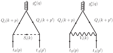
Figure 2: In the left diagram, the interactions of the SM top and the BLHM heavy quarks $Q=(T,T^{5},T^{6},T^{2/3},T^{5/3},B)$ with scalar fields $S_{k}$ are depicted: $A^{0},H^{0},h^{0},H^{\pm},\phi^{0},\eta^{0},\sigma,\phi^{\pm},\eta^{\pm}$. In the right diagram, the interactions of the same quarks with vector fields $V_{k}$ are illustrated: $Z^{0},W^{\pm},\gamma,Z^{\prime},W^{\prime\pm}$.

V Phenomenology of the CMDM

In the context of the CMDM, the valid one-loop diagrams with scalar and vector contributions are shown in Fig. 2. The amplitudes corresponding to the diagrams are given by:

$$\mathcal{M}^{\mu}_{t}(S)=\sum_{i,j}\int\frac{d^{4}k}{(2\pi)^{4}}\bar{u}(p^{\prime})(S^{\ast}_{j}+P^{\ast}_{j}\gamma^{5})\delta_{A\alpha_{1}}$$ (54)

$$\times\left[i\frac{\not{k}+\not{p}^{\prime}+m_{Q_{j}}}{(k+p^{\prime})^{2}-m_{Q_{j}}^{2}}\delta_{\alpha_{1}\alpha_{3}}\right]\left(-ig_{s}\gamma^{\mu}T^{a}_{\alpha_{2}\alpha_{3}}\right)$$

$$\times\left[i\frac{\not{k}+\not{p}+m_{Q_{j}}}{(k+p)^{2}-m^{2}_{Q_{j}}}\right](S_{j}+P_{j}\gamma^{5})\delta_{B\alpha_{4}}u(p)$$

$$\times\left(\frac{i}{k^{2}-m^{2}_{S_{i}}}\right)V_{Ht}^{\ast}V_{Ht},$$

and

$$\mathcal{M}^{\mu}_{t}(V)=\sum_{i,j}\int\frac{d^{4}k}{(2\pi)^{4}}\bar{u}(p^{\prime})\gamma^{a_{1}}(V^{\ast}_{j}+A^{\ast}_{j}\gamma^{5})\delta_{A\alpha_{1}}$$ (55)

$$\times\left[i\frac{\not{k}+\not{p}^{\prime}+m_{Q_{j}}}{(k+p^{\prime})^{2}-m_{Q_{j}}^{2}}\delta_{\alpha_{1}\alpha_{3}}\right]\left(-ig_{s}\gamma^{\mu}T^{a}_{\alpha_{2}\alpha_{3}}\right)$$

$$\times\left[i\frac{\not{k}+\not{p}+m_{Q_{j}}}{(k+p)^{2}-m^{2}_{Q_{j}}}\right]\gamma^{a_{2}}(V_{j}+A_{j}\gamma^{5})\delta_{B\alpha_{4}}u(p)$$

$$\times\left[\frac{i}{k^{2}-m^{2}_{V_{i}}}\left(-g_{\alpha_{1}\alpha_{2}}+\frac{k_{\alpha_{1}}k_{\alpha_{2}}}{m^{2}_{V_{i}}}\right)\right]V^{\ast}_{Ht}V_{Ht},$$

where $T^{a}_{\alpha_{n}\alpha_{m}}$ are the $SU(3)$ generators. The coefficients $(S_{j},P_{j},V_{j},A_{j})$ carry all contributions from the BLHM quantified by the vertices $\bar{Q}_{j}S_{i}t$, $\bar{t}S_{i}^{\dagger}Q_{j}$ for scalar and pseudoscalar interactions, and $\bar{Q}_{j}V_{i}t$, $\bar{t}V_{i}^{\dagger}Q_{j}$ for vector and axial interactions, respectively. The matrix elements $V^{\ast}_{Ht}V_{Ht}$ belong to the extended CKM matrix $V_{Hu}$. To compute the amplitudes (54) and (55), we used the FeynCalc package [42] and the Package X [43] for Mathematica.

In interactions with charged bosons, both scalar and vector, it is necessary to consider the extended CKM matrix for the BLHM, $V_{CKM}=V_{Hu}^{\dagger}V_{Hd}$, introduced in [3], where the unitary matrix $V_{Hu}^{\dagger}$ represents transitions from heavy quarks to light up-type quarks, and $V_{Hd}$ represents transitions from heavy quarks to light down-type quarks. We can generalize the CKM extended matrix like the product of three rotations matrices [40, 41]

$$V_{Hd}\; =\begin{pmatrix}1&0&0\\ 0&c_{23}^{d}&s_{23}e^{-i\delta_{23}^{d}}\\ 0&-s_{23}^{d}e^{i\delta_{23}^{d}}&c_{23}^{d}\end{pmatrix}$$

$$\times\begin{pmatrix}c_{13}^{d}&0&s_{13}^{d}e^{-i\delta_{13}^{d}}\\ 0&1&0\\ -s_{13}e^{i\delta_{13}^{d}}&0&c_{13}^{d}\end{pmatrix}$$

$$\times\begin{pmatrix}c_{12}^{d}&s_{12}^{d}e^{-i\delta_{12}^{d}}&0\\ -s_{12}^{d}e^{i\delta_{12}^{d}}&c_{12}^{d}&0\\ 0&0&1\end{pmatrix}.$$

Where the $c^{d}_{ij}$ and $s^{d}_{ij}$ are in terms of the angles $(\theta_{12},\theta_{23},\theta_{13})$ and the phases $(\delta_{12},\delta_{23},\delta_{13})$.

We have considered three cases for the extended matrices:

Case I. $V_{Hu}=\mathbf{1}$, this implies $V_{Hd}=V_{CKM}^{\dagger}$.

Case II. $V_{Hd}=\mathbf{1}$, this implies $V_{Hu}=V_{CKM}^{\dagger}$.

Case III. $s_{23}^{d}=1/\sqrt{2}$, $s_{12}^{d}=s_{13}^{d}=0$, $\delta_{12}^{d}=\delta_{23}^{d}=\delta_{13}^{d}=0$. Substituting the values of case III into the matrix $V_{Hd}$ in Eq. (V), we obtain the matrix:

$$V_{Hd}=\begin{pmatrix}1&0&0\\ 0&1&1/\sqrt{2}\\ 0&-1/\sqrt{2}&1\end{pmatrix},$$ (57)

and through the product $V_{Hd}V_{CKM}^{\dagger}$, we obtain the matrix $V_{Hu}$ =

$$\left(\begin{matrix}0.9737\pm 0.0003&0.221\pm 0.004&0.0086\pm 0.0002\\ 0.227\pm 0.0008&1.0038\pm 0.0061&0.7585\pm 0.0206\\ -0.1548\pm 0.0006&-0.6486\pm 0.0045&0.9847\pm 0.0291\end{matrix}\right)$$ (58)

where the uncertainties are computed analytically using the reported experimental uncertainties of the CKM-matrix elements. The latter are found in Table 5.

Finally, to obtain the total contribution of the BLHM to the chromomagnetic dipole, we sum the scalar and vectorial contributions given by the amplitudes of Eqs. (54) and (55). The computation of $\hat{\mu}_{t}^{BLHM}$ involves several measured boson and quark masses. Since these experimental results are reported with statistical and systematic uncertainties, becomes essential to propagate them into our calculations. Moreover, the BLHM introduces the free model parameters $y_{1},\;y_{2},\;y_{3}$ and $\alpha$, we adopt a conservative approach and assign them an uncertainty of 1%. Therefore to include these uncertainties, we carried out a statistical simulation of error propagation: We randomly sampled the experimental masses and parameters from a Gaussian probability distribution with a mean equal to their central value and a width equal to the squared sum of the uncertainties. We calculated $\hat{\mu}_{t}^{BLHM}$ using sampled masses and parameters corresponding to the experimentally observed masses and the given values for the BLHM parameters. We repeated the procedure $10^{4}$ times. In this manner, we obtained a Gaussian distribution for the $\hat{\mu}_{t}^{BLHM}$. Next, we assigned the mean of the distribution as the value of the parameter and used its difference from the distribution quantiles at 68% and 95% confidence level (C.L.), in order to extract the 68% and 95% confidence intervals (C.I.). The latter allows for asymmetric uncertainties. This method is known as the Monte Carlo bootstrap uncertainty propagation [46, 47]. Table 5 displays the masses and parameters of the model along with the experimental uncertainties, either directly from the reported value or calculated using standard analytic error propagation. In Table 5, the experimentally measured values found are reported by the Particle Data Group [48].

Table 5: Masses and parameters with uncertainties used in the calculation of the $\hat{\mu}_{t}^{BLHM}$.

Parameter	Value
$m_{Z}$	$91.1876\pm 0.0021$ GeV
$m_{W}$	$80.377\pm 0.012$ GeV
$m_{H_{0}}$	$125.11\pm 0.11$ GeV
$m_{t}$	$172.76\pm 0.3$ GeV
$m_{b}$	$4.18\pm 0.00045$ GeV
$g$	$0.6258\pm 0.001$
$g^{\prime}$	$0.3528\pm 0.001$
$|V_{ud}|$	$0.97373\pm 0.00031$
$|V_{us}|$	$0.2243\pm 0.0008$
$|V_{ub}|$	$0.00382\pm 0.00020$
$|V_{cd}|$	$0.221\pm 0.004$
$|V_{cs}|$	$0.975\pm 0.006$
$|V_{cb}|$	$0.0408\pm 0.0014$
$|V_{td}|$	$0.0086\pm 0.0002$
$|V_{ts}|$	$0.0415\pm 0.0009$
$|V_{tb}|$	$1.014\pm 0.029$
$v$	$246.22\pm(6.06\times 10^{-12})$ GeV
$y_{1}$	$0.7\pm 0.01$
$y_{2}$	$0.9\pm 0.01$
$y_{3}$	$0.01\pm 0.001$
$\alpha$	$-1.67081\pm 0.001$

VI Results

This section presents our results for the $\hat{\mu}_{t}^{BLHM}$ calculations. Figs. 3-5 condense the results for all the studied $\beta$ angles for Cases I, II, and III described in subsections VI.1, VI.2, VI.3, respectively. In Appendix B, we provide an individual plot of each $\beta$ considered to show the 68% and 95% confidence interval bands, which arise from propagating the experimental and model parameter uncertainties. These plots are shown in Figs. 7, 8, 9 and correspond to Cases I, II, III, respectively. In Table 6, we summarize the numerical values our $\hat{\mu}_{t}^{BLHM}$ calculations along with their uncertainty at 68% C.L.

VI.1 Case I

In Fig. 3, we present the CMDM, $\hat{\mu}_{t}$, for the first case of the extended CKM matrix with $V_{Hu}=\mathbf{1}$ and $1<f<3$ TeV. The scalar contributions to these dipoles are positive of order $10^{-4}$, while the vectorial contributions were positive also of order $10^{-4}$. As we can observe, the vectorial contributions dominate in the total CMDM, which is positive for the entire range of the scale $f$. Fig. 3 displays the results for the $\beta=0.79,0.94,1.09,1.23,1.47$ angles. Here, only the central values of $\hat{\mu}_{t}$ are shown; we do not show their uncertainties. The values of $\hat{\mu}_{t}^{BLHM}$ with uncertainties are found in Fig. 7 of Appendix B, which show the central value and its confidence intervals.

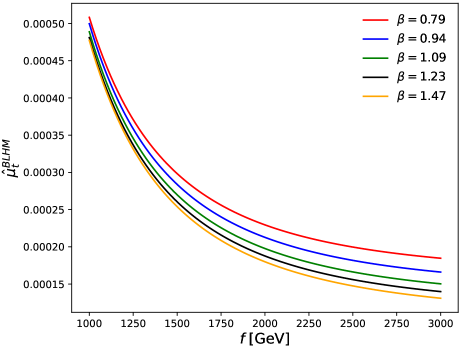
Figure 3: Case I. Total contributions to the CMDMs with the CKM matrix $V_{Hu}=\mathbf{1}$.

VI.2 Case II

In Fig. 4, we present the CMDMs for the second case with the extended CKM matrix $V_{Hu}=V_{CKM}^{\dagger}$. The scalar contributions were positive of order $10^{-6}$, while the vectorial contributions were positive of order $10^{-4}$. We can observe from the plot that the total CMDMs are positive for the same angles $\beta$ as in the first case and also of order $10^{-4}$. Fig. 4 displays the results for the $\beta=0.79,0.94,1.09,1.23,1.47$ angles. Here, only the central values of $\hat{\mu}_{t}$ are shown; we do not show their uncertainties. The values of $\hat{\mu}_{t}^{BLHM}$ with uncertainties are found in Fig. 8 of Appendix B, which show the central value and its confidence intervals.

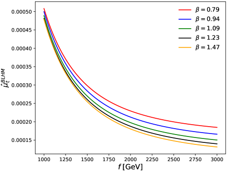
Figure 4: Case II. Total contributions to the CMDMs with the CKM matrix $V_{Hu}=V_{CKM}^{\dagger}$.

VI.3 Case III

In Fig. 5, we show the curves corresponding to the CMDMs with the extended CKM matrix of Eq. (58). The scalar contributions were only positive of order $10^{-6}$, while the vectorial contributions were both positive and negative of order $10^{-4}$. However, the numerical values of $\hat{\mu}_{t}$ turned out to be almost equal to those of the second and third cases due to the small difference between the matrix elements $V_{Hu}(3,3)$ of the three extended matrices. Fig. 4 displays the results for the $\beta=0.79,0.94,1.09,1.23,1.47$ angles. Here, only the central values of $\hat{\mu}_{t}$ are shown. That is, we do not show their uncertainties. The values of $\hat{\mu}_{t}^{BLHM}$ with uncertainties are found in Fig. 9 of Appendix B, which show the central value and its confidence intervals.

Figure 5: Case III. Total contributions to the CMDMs with the CKM matrix of Eq. (58) for the $\beta$ angles considered. The solid lines correspond to the central values of our calculations.

Table 6: Numerical values of the CMDM for the three cases of the extended CKM matrix. In the first column the $\beta$ angles are indicated. The second column contains the values for the CMDM evaluated at $f=1$ TeV. The third column contains the values for the CMDM evaluated at $f=3$ TeV. The uncertainties are reported at 68% C.L.

	Case I	Case I
$\beta$ [rad]	$f=1$ TeV	$f=3$ TeV
$0.79$	$(5.09^{+0.14}_{-0.12})\times 10^{-4}$	$(1.85^{+0.04}_{-0.04})\times 10^{-4}$
$0.94$	$(5.00^{+0.18}_{-0.16})\times 10^{-4}$	$(1.66^{+0.06}_{-0.06})\times 10^{-4}$
1.09	$(4.89^{+0.21}_{-0.18})\times 10^{-4}$	$(1.5^{+0.07}_{-0.06})\times 10^{-4}$
1.23	$(4.81^{+0.23}_{-0.20})\times 10^{-4}$	$(1.39^{+0.08}_{-0.07})\times 10^{-4}$
1.47	$(4.77^{+0.24}_{-0.21})\times 10^{-4}$	$(1.31^{+0.08}_{-0.07})\times 10^{-4}$
	Case II	Case II
$\beta$ [rad]	$f=1$ TeV	$f=3$ TeV
$0.79$	$(5.09^{+0.13}_{-0.12})\times 10^{-4}$	$(1.85^{+0.04}_{-0.04})\times 10^{-4}$
$0.94$	$(5.00^{+0.18}_{-0.16})\times 10^{-4}$	$(1.66^{+0.06}_{-0.06})\times 10^{-4}$
1.09	$(4.87^{+0.21}_{-0.18})\times 10^{-4}$	$(1.5^{+0.07}_{-0.06})\times 10^{-4}$
1.23	$(4.81^{+0.23}_{-0.20})\times 10^{-4}$	$(1.39^{+0.08}_{-0.07})\times 10^{-4}$
1.47	$(4.79^{+0.21}_{-0.20})\times 10^{-4}$	$(1.32^{+0.07}_{-0.07})\times 10^{-4}$
	Case III	Case III
$\beta$ [rad]	$f=1$ TeV	$f=3$ TeV
$0.79$	$(5.08^{+0.13}_{-0.12})\times 10^{-4}$	$(1.85^{+0.04}_{-0.04})\times 10^{-4}$
$0.94$	$(4.98^{+0.18}_{-0.16})\times 10^{-4}$	$(1.66^{+0.06}_{-0.06})\times 10^{-4}$
1.09	$(4.87^{+0.21}_{-0.18})\times 10^{-4}$	$(1.5^{+0.07}_{-0.06})\times 10^{-4}$
1.23	$(4.81^{+0.23}_{-0.20})\times 10^{-4}$	$(1.39^{+0.08}_{-0.07})\times 10^{-4}$
1.47	$(4.77^{+0.22}_{-0.23})\times 10^{-4}$	$(1.32^{+0.08}_{-0.07})\times 10^{-4}$

Table 6 displays the numerical values for the CMDM according to $f=1,3$ TeV. As previously stated, these values are expected to be nearly identical across all three cases, up to two decimal points. However, differences become apparent when examining values to a greater number of decimal points.

The CMDM of the SM was computed off-shell in [44, 45] in both its spacelike version $\hat{\mu}_{t}=-0.0224-0.000925i$ and timelike version $\hat{\mu}_{t}=-0.0133-0.0267i$. We have also computed the CMDM by taking the off-shell gluon $(q^{2}\neq 0)$ in the two scenarios: the spacelike $(q^{2}=-m^{2}_{Z})$ and the timelike one $(q^{2}=m_{Z}^{2})$. In our case, the CMDMs turned out to be identical for both scenarios due to the equality $g_{A}=g_{B}$ between the coupling constants of the $SU(2)_{A}$ and $SU(2)_{B}$ groups, respectively.

VI.4 Special case

We had set constraints on the parameter space of the BLHM based on conditions to minimize corrections on the Higgs and keep the fine-tuning, $\Psi$, below $\Psi=2$. Consequently, the interval for the mixing angle $\beta$ was narrowed down to $0.79<\beta<1.47$ radians. However, in Fig. 6, we show the plot of the total CMDM for the mixing angle $\beta=0.1559$ and $V_{Hu}=1$, which approximately reproduces the experimental result with the value $\hat{\mu}_{t}=-0.02427$ for $f=1$ TeV. Below $\beta=0.79$ rad, there are several $\hat{\mu}(f)_{t}$ values that also reproduce the SM $\hat{\mu}_{t}^{Exp}$ for some $f\in[1,3]$ TeV. Thus, we have magnitudes of the order of $10^{-2}$ for the CMDM in ranges not allowed for $\beta$.

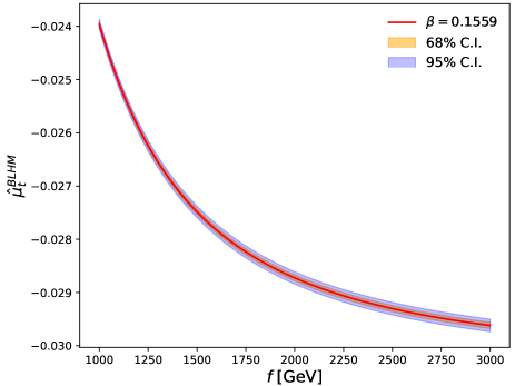
Figure 6: Special case. Total contributions to the CMDM for $\beta=0.1559$. The solid red line corresponds to the central value of our calculation. The orange and blue bands are the 68% and 95% C.I., respectively, which arise from the uncertainty propagation described in Sec.V.

VII Conclusions

In this work, we calculate the CMDM for different values of the mixing angle $\beta$, finding values on the order of $10^{-4}-10^{-2}$ within the allowed interval for the parameter space due to the constraints on the corrections received by the Higgs and the fine-tuning. We also present a special case in which we use smaller values for $\beta$ and $V_{Hu}=1$, such that the model directly reproduces the experimental value of the SM, $\hat{\mu}_{t}^{Exp}=-0.024$. In this study, we introduced for the first time the extended CKM matrix for the case of chromomagnetic dipole in the BLHM. In the first case, the matrix $V_{Hu}=\mathbf{1}$ show us that $\hat{\mu}_{t}$, as can be observed in Fig. 3, has positive values for the CMDM. In the second case, the matrix $V_{Hu}=V^{\dagger}_{CKM}$ has no significant effects on the shape of the chromodipoles or their orders of magnitude. In the last case, the matrix $V_{Hu}$ given by Eq. (58) also has no important effects on the total CMDMs, such that they are almost equal to those of the first and second case at first glance. It is important to note that the contributions involving the matrix elements $V_{Hu}$ are very few because we have only quantified the interactions of the top quark and the charged bosons with virtual heavy quarks in the BLHM. That is, only the heavy quarks $B$ and $T^{5/3}$ have intervened on a few occasions. Another important aspect is the equality of the CMDMs calculated in the spacelike and timelike scenarios due to the equality between the coupling constants of the $SU(2)_{A}$ and $SU(2)_{B}$ groups, so that these parameters can be adjusted to obtain different results. Regarding the experimental aspect, given the most recent value of the CMDM [13], our results on the order of $10^{-4}$ may compete within the reported uncertainty; however, theoretical adjustments in the BLHM could still be made to improve the order of magnitude of $\hat{\mu}_{t}$. Finally, it is worth mentioning that we thoroughly propagated all sources of uncertainties to compute uncertainty bands in our calculations of the CMDM. This uncertainty information may be relevant to help guide future theory, phenomenological, and experimental research at present and future particle colliders.

Appendix A Feynman rules in the BLHM

In this appendix we present the Feynman rules for the BLHM necessary to calculate the CMDM.

Tables 7–9 summarize the Feynman rules for the 3-point interactions: fermion-fermion-scalar (FFS), fermion-fermion-gauge (FFV), gauge-gauge-gauge (VVV), and scalar-gauge-gauge (SVV) interactions.

Table 7: Essential Feynman rules in the BLHM for studying the CMDM.

Vertex	Rule (Factors in Tables 8 and 9)
$W^{\prime-}\bar{B}t$	$\dfrac{-igs_{\beta}v}{4\sqrt{2}f}A_{y}\gamma^{\mu}P_{L}(V_{Hu})$
$\eta^{-}\bar{B}t$	$\dfrac{4im_{W}^{2}}{f^{2}g^{2}\sqrt{y_{1}^{2}+y_{2}^{2}}(y_{1}^{2}+y_{3}^{2})}(Y_{1}P_{L}+Y_{2}P_{R})(V_{Hu})$
$\phi^{-}\bar{B}t$	$F_{a}F_{b}(X_{1}P_{L}+X_{2}P_{R})(V_{Hu})$
$H^{-}\bar{B}t$	$\dfrac{-3\sqrt{2}m_{W}c_{\beta}s_{\beta}y_{1}y_{2}y_{3}^{2}}{fg\sqrt{y_{1}^{2}+y_{2}^{2}}(y_{1}^{2}+y_{3}^{2})}P_{L}(V_{Hu})$

Table 8: Factors from Table 7.

Factor	Expression
$A_{y}$	$y_{3}(2y_{1}^{2}-y_{2}^{2})(y_{1}^{2}+y_{2}^{2})^{2}(y_{1}^{2}+y_{3}^{2})$
$Y_{1}$	$B_{1}+B_{2}$
$Y_{2}$	$B_{3}+B_{4}$
$F_{a}$	$\dfrac{y_{3}(2y_{1}^{2}-y_{2}^{2})}{(y_{1}^{2}+y_{3}^{2})\sqrt{y_{1}^{2}+y_{2}^{2}}}$
$F_{b}$	$\dfrac{Fs_{\beta}}{2f\sqrt{2(f^{2}+F^{2})}}$
$X_{1}$	$A_{1}+A_{3}+A_{6}$
$X_{2}$	$A_{2}+A_{4}+A_{5}$

Table 9: Factors from Table 8.

$B_{1}$	$y_{1}y_{2}(y_{1}^{2}+y_{3}^{2})c_{\beta}^{2}$
$B_{2}$	$y_{1}^{3}y_{2}s_{\beta}-\dfrac{1}{2}y_{1}y_{2}y_{3}^{2}s_{\beta}$
$B_{3}$	$\dfrac{fg}{4m_{W}}y_{3}(2y_{1}^{2}+5y_{2}^{2})\sqrt{y_{1}^{2}+y_{3}^{2}}s_{\beta}$
$B_{4}$	$-y_{1}^{3}y_{3}s_{\beta}-\dfrac{1}{2}y_{1}(y_{2}^{2}+y_{3}^{2})s_{\beta}$
$A_{1}$	$\dfrac{-4m_{W}c_{\beta}^{2}y_{1}y_{2}(y_{1}^{2}+y_{3}^{2})}{s_{\beta}y_{3}(2y_{1}^{2}-y_{2}^{2})}$
$A_{2}$	$fg-y_{1}^{8}-m_{W}s_{\beta}y_{3}y_{2}^{6}-3y_{2}y_{1}^{4}(2y_{1}^{2}-y_{2}^{2})$
	$-y_{1}^{6}(3y_{2}^{2}+y_{3}^{2})-y_{1}^{2}y_{2}^{4}(y_{2}^{2}+3y_{3}^{2})$
$A_{3}$	$\dfrac{-4m_{W}y_{1}^{3}y_{2}y_{3}}{2y_{1}^{2}-y_{2}^{2}}$
$A_{4}$	$\dfrac{8m_{W}y_{1}^{3}(y_{2}^{2}+y_{3}^{2})}{2y_{1}^{2}-y_{2}^{2}}$
$A_{5}$	$\dfrac{-4m_{W}y_{1}^{3}}{2y_{1}^{2}-y_{2}^{2}}$
$A_{6}$	$\dfrac{4m_{W}y_{1}^{3}y_{2}}{y_{3}(2y_{1}^{2}-y_{2}^{2})}$

Appendix B Individual $\mu_{t}^{BHLM}$ plots

In this appendix we present the individual plots of the $\hat{\mu}_{t}^{BHLM}$ for the different $\beta$ angles. These plots are intended to ease the display of the confidence intervals in our calculations. Fig. 7 shows the $\hat{\mu}_{t}^{BHLM}$ for Case I as discussed in Section VI.1. Fig. 8 shows the $\hat{\mu}_{t}^{BHLM}$ for Case II as discussed in Section VI.2. Fig. 9 shows the $\hat{\mu}_{t}^{BHLM}$ for Case III as discussed in Section VI.3.

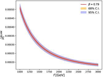
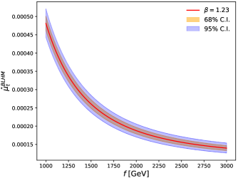
Figure 7: Case I. Total contributions to the CMDM for $\beta$ angle indicated in each plot. The solid red line corresponds to the central value of our calculation. The orange and blue bands are the 68% and 95% C.I., respectively, which arise from the uncertainty propagation described in Sec.V.

Figure 8: Same as Fig. 7, but for Case II.

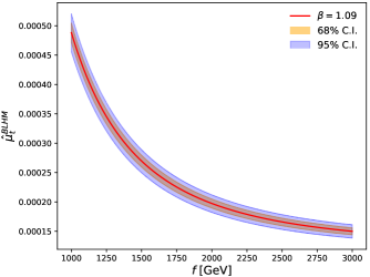
Figure 9: Same as Fig. 7, but for Case III.

References

- [1] M. Schmaltz, D. Stolarski and J. Thaler, JHEP 09, 018 (2010).
- [2] J. I. Aranda, T. Cisneros-Pérez, E. Cruz-Albaro, J. Montaño-Domínguez and F. Ramírez-Zavaleta. arXiv:2111.03180 [hep-ph].
- [3] T. Cisneros-Pérez, M. A. Hernández-Ruíz, A. Gutiérrez-Rodríguez, E. Cruz-Albaro, Eur. Phys. J. C 83, 1093 (2023).
- [4] M. Kobayashi and T. Maskawa, Prog. Theor. Phys. 49, 652 (1973).
- [5] R. Martinez, M. A. Perez and N. Poveda, Eur. Phys. J. C 53, 221-230 (2008).
- [6] L. Ding and C. X. Yue, Commun. Theor. Phys. 50, 441-444 (2008).
- [7] A. I. Hernández-Juárez, G. Tavares-Velasco and A. Moyotl, Chin. Phys. C 45, 113101 (2021).
- [8] D. Buarque Franzosi and C. Zhang, Phys. Rev. D 91, 114010 (2015).
- [9] J. I. Aranda, T. Cisneros-Pérez, J. Montaño, B. Quezadas-Vivian, F. Ramírez-Zavaleta and E. S. Tututi, Eur. Phys. J. Plus 136, 164 (2021).
- [10] E. Cruz-Albaro and A. Gutiérrez-Rodríguez, Eur. Phys. J. Plus 137, 1295 (2022).
- [11] E. Cruz-Albaro, A. Gutiérrez-Rodríguez, J. I. Aranda and F. Ramírez-Zavaleta, Eur. Phys. J. C 82, 1095 (2022).
- [12] E. Cruz-Albaro, A. Gutierrez-Rodrıguez, M. A. Hernandez-Ruız and T. Cisneros-Perez, Eur. Phys. J. Plus 138, 506 (2023).
- [13] Sirunyan, A., et al., JHEP 06, 146 (2020).
- [14] R. Martinez and J. A. Rodriguez, Phys. Rev. D 55, 3212-3214 (1997).
- [15] R. Martinez and J. A. Rodriguez, Phys. Rev. D 65, 057301 (2002).
- [16] A. I. Hernández-Juárez, A. Moyotl and G. Tavares-Velasco, Phys. Rev. D 98, 035040 (2018).
- [17] M. Schmaltz and J. Thaler, JHEP 03, 137 (2009).
- [18] Moats, K. doi: 10.22215/etd/2012-09748, (2012).
- [19] T. A. W. Martin. doi:10.22215/etd/2012-09697, (2012).
- [20] S. Godfrey, T. Gregoire, P. Kalyniak, T. A. W. Martin and K. Moats, JHEP 04, 032 (2012).
- [21] P. Kalyniak, T. Martin and K. Moats, Phys. Rev. D 91, 013010 (2015).
- [22] A. Tumasyan et al. [CMS], JHEP 12, 161 (2021).
- [23] A. M. Sirunyan et al. [CMS], Phys. Lett. B 805 (2020), 135425
- [24] G. Aad et al. [ATLAS], Eur. Phys. J. C 81, 396 (2021).
- [25] G. Aad et al. (ATLAS Collaboration), Phys. Lett. B744, 163 (2015).
- [26] A. M. Sirunyan et al. (CMS Collaboration), JHEP 03, 055 (2020).
- [27] M. Hashemi and G. Haghighat, Eur. Phys. J. C 79, 419 (2019).
- [28] A. Tumasyan et al. (CMS Collaboration), JHEP 09, 032 (2023).
- [29] G. Aad et al. [ATLAS], JHEP 06, 145 (2021).
- [30] Wells, J. Physical Review D 107, 055022 (2023).
- [31] D. Buttazzo, A. Greljo and D. Marzocca, Eur. Phys. J. C 76, 116 (2016).
- [32] U. Haisch, G. Polesello and S. Schulte, JHEP 09, 206 (2021).
- [33] G. Aad et al. (ATLAS Collaboration), JHEP 08, 153 (2023).
- [34] G. Aad et al. (ATLAS Collaboration), Eur. Phys. J. C 83, 719 (2023).
- [35] M. Aaboud et al. [ATLAS], JHEP 07, 089 (2018).
- [36] A. M. Sirunyan et al. [CMS], JHEP 08, 177 (2018).
- [37] A. Tumasyan et al. [CMS], JHEP 09, 051 (2023).
- [38] A. Tumasyan et al. [CMS], Phys. Rev. D 105, 032008 (2022).
- [39] A. M. Sirunyan et al. [CMS], Eur. Phys. J. C 81, 688 (2021).
- [40] M. Blanke, A. J. Buras, A. Poschenrieder, S. Recksiegel, C. Tarantino, S. Uhlig and A. Weiler, Phys. Lett. B646, 253 (2007).
- [41] M. Blanke, A. J. Buras, A. Poschenrieder, S. Recksiegel, C. Tarantino, S. Uhlig and A. Weiler, JHEP 01, 066 (2007).
- [42] V. Shtabovenko, R. Mertig and F. Orellana, Comput. Phys. Commun. 256, 107478 (2020).
- [43] H. H. Patel, Comput. Phys. Commun. 218, 66 (2017).
- [44] J. I. Aranda, D. Espinosa-Gómez, J. Montaño, B. Quezadas-Vivian, F. Ramírez-Zavaleta and E. S. Tututi, Phys. Rev. D 98, 116003 (2018).
- [45] J. I. Aranda, T. Cisneros-Pérez, J. Montaño, B. Quezadas-Vivian, F. Ramírez-Zavaleta and E. S. Tututi, Eur. Phys. J. Plus 136, 164 (2021).
- [46] B. Efron, R.J. Tibshirani, Mono. Stat. Appl. Probab. Chapman and Hall, London, (1993).
- [47] D. Molina, M. De Sanctis, C. Fernández-Ramírez and E. Santopinto, Eur. Phys. J. C 80, 526 (2020).
- [48] R. L. Workman et al. [Particle Data Group], PTEP 2022, 083C01 (2022).