An Improved Framework for Computing Waveforms

Abstract

We combine the observable-based formalism (KMOC), the analytic properties of the scattering amplitude, generalised unitarity and the heavy-mass expansion with a newly introduced IBP reduction for Fourier integrals, to provide an efficient framework for computing scattering waveforms. We apply this framework to the scattering of two charged massive bodies in classical electrodynamics. Our work paves the way for the computation of the analytic one-loop waveform in General Relativity.

1 Introduction

The emission of GWs emitted by a gravitating binary system has been studied for a long time in General Relativity, starting from the original leading-order quadrupole formula provided by Einstein Einstein:1918btx , and from the pioneering computations of Kovacs and Thorne, and of Peters Peters:1970mx ; Kovacs:1977uw ; Kovacs:1978eu . The Multipolar-Post-Minskowskian formalism (MPM) Blanchet:1985sp ; Blanchet:1989ki ; Blanchet:2004ek has been one of the most effective methods for computing analytically the GWs emission from generic sources at very high precision for bound and unbound systems Blanchet:2023bwj ; Blanchet:2023sbv ; Bini:2023fiz ; Bini:2024rsy . A novel framework to study the relativistic two-body problem emerged from particle physics and is based on effective field theories (EFTs) reasoning Goldberger:2004jt . Classical bodies are studied in an EFT approach as point particles interacting via the exchange of gravitons, and their internal structure, such as spin and tidal forces, is encoded in non-minimal coupling to the gravitational field.

Classical in-in observables are directly related to scattering amplitudes via an observable-based approach (KMOC formalism) Kosower:2018adc , reviewed in section 2. Within this framework, the waveform can be connected to the Fourier transform (FT) of $2\to 3$ scattering amplitudes Cristofoli:2021vyo , after suitably changing some $i\epsilon$ prescriptions Caron-Huot:2023vxl .

The computation of the amplitudes is simplified by taking the classical expansion at the integrand level, before integrating over the loop momenta and taking the FT. Exploiting the method of regions Beneke:1997zp , the classical regime can be identified with the so-called soft region Cheung:2018wkq ; Bern:2019nnu ; Bern:2019crd , which corresponds to long-range interactions mediated by internal gravitons, where the loop momenta scales as the transferred and radiated momenta ($q$ and $k$, respectively): $\ell\sim q\sim k\ll m$. Alternatively, this classical limit can be performed as a heavy-mass expansion Brandhuber:2021kpo ; Brandhuber:2021eyq . The construction of the integrand can be further simplified by borrowing tools from generalised unitarity Bern:1994zx ; Bern:1994cg ; Bern:1995db ; Britto:2004nc ; Britto:2005ha ; Britto:2006sj ; Anastasiou:2006jv ; Ossola:2006us ; Anastasiou:2006gt . The integration instead is made possible by powerful methods developed in precision physics for multi-loop computations, such as integration-by-parts identities (IBPs) Tkachov:1981wb ; Chetyrkin:1981qh ; Laporta:2000dsw ; Smirnov:2008iw ; Maierhofer:2017gsa ; Lee:2012cn – which allow reducing all Feynman integrals (FIs) for a process in terms of a minimal set of linearly-independent integrals, known as Master Integrals (MIs) –, and differential equations (DEs) Kotikov:1990kg ; Remiddi:1997ny ; Gehrmann:1999as ; Argeri:2007up ; Henn:2013pwa ; Henn:2014qga ; Argeri:2014qva ; Lee:2014ioa . Using these tools, the waveform has been computed at tree level for spinless particles using worldline formalism Jakobsen:2021smu ; Mougiakakos:2021ckm and including spin corrections Jakobsen:2021lvp ; DeAngelis:2023lvf ; Brandhuber:2023hhl ; Aoude:2023dui . The computation has been extended to the one-loop order and spinless bodies Brandhuber:2023hhy ; Herderschee:2023fxh ; Georgoudis:2023lgf ; Elkhidir:2023dco ; Caron-Huot:2023vxl , and including linear-in-spin corrections Bohnenblust:2023qmy . It has recently found agreement with Multipolar Post-Minkowskian (MPM) formalism in the small velocity expansion Bini:2023fiz ; Georgoudis:2023eke ; Bini:2024rsy ; Georgoudis:2024pdz . The one-loop amplitude contains many terms and spurious poles Brandhuber:2023hhy ; Herderschee:2023fxh ; Bohnenblust:2023qmy (Gram determinant poles appearing from the reduction of tensor integrals), making it hard to think of an analytic evaluation of the FT – for example, the small-velocity expansion was only possible via a cumbersome reorganisation of the different terms appearing Bini:2024rsy .

The main goal of this work is to provide an efficient framework to compute the analytic waveform, treating the FT and the loop integrals as a genuine two-loop integration. The study of the analytic and algebraic properties of these Fourier-loop (FL) integrals will allow us to avoid the appearance of these poles in intermediate steps. Improvements can be made on several levels.

1. Integrand. From the analytic properties of the FL integrals, it is possible to select only the contributions to the amplitude giving rise to long-range interactions in the classical limit, discarding all contact terms. In the classical regime, only singularities related to internal on-shell gravitons survive. When we consider the Fourier integral of a function, we can exploit Cauchy’s theorem to select these contributions, which can be treated as generalised unitarity cuts Kosower:2011ty ; Badger:2012dv ; Mastrolia:2012an ; Ita:2015tya ; Bourjaily:2015jna . The building blocks fed into the cuts are computed in the heavy-mass expansions.

2. Spurious poles. We perform the tensor decomposition at the level of the full FL integral, thus bypassing the problem of spurious poles.

3. Integral reduction. FIs of a given family live in a finite-dimensional vector space and the coefficients of the IBP decomposition of a given FI into a basis can be obtained from their intersection numbers Mastrolia:2018uzb ; Frellesvig:2019uqt . Integrals containing an exponential factor such as FTs can be analysed in the same spirit: this has been first seen in the context of confluent hypergeometric functions Matsumoto1998-2 ; majima2000 , and recently in relevant physical applications Cacciatori:2022mbi ; Brunello:2023fef . Hence, Fourier integrals can be decomposed into a basis of MIs. This will leave us with the evaluation of a few integrals, which are the FTs of the scalar one-loop MIs.

We evaluate for the first time the analytic one-loop waveform in classical electrodynamics for arbitrary velocities, paving the way for the analogous calculation in General Relativity, that will be presented elsewhere Brunello:toappear .

2 Classical observables and Analyticity beyond the Physical Region

2.1 KMOC and the Waveform

We start by reviewing the observable-based formalism (KMOC) Kosower:2018adc ; Cristofoli:2021vyo ; Caron-Huot:2023vxl for computing (classical) in-in observables from QFT scattering amplitudes. In general, we are interested in computing asymptotic observables, i.e. the expectation value of some observable in the far future, after preparing the initial state of the system $|\psi\rangle_{\rm in}$ in the far past. We let the state transform with time and the evolution from the far past to the far future is given by the unitarity $S$ operator. We are generally interested in measuring the variation of the system:

$$\Delta\langle\mathcal{O}\rangle=\langle\mathcal{O}\rangle_{\rm out}-\langle\mathcal{O}\rangle_{\rm in}=\,_{\rm out}\langle\psi|\mathcal{O}|\psi\rangle_{\rm out}-\,_{\rm in}\langle\psi|\mathcal{O}|\psi\rangle_{\rm in}=\,_{\rm in}\langle\psi|S^{\dagger}[\mathcal{O},S]|\psi\rangle_{\rm in}\ ,$$ (1)

with

$$S^{\dagger}S=\mathbf{1}\ .$$ (2)

The KMOC formalism has been developed in the context of the (classical) two-body problem in gravity and electrodynamics. In this case, we consider $|\psi\rangle_{\rm in}$ to be a two-particle state, integrated against an on-shell wavefunction. Then, the initial state is

$$|\psi\rangle_{\rm in}=\int\!\!\mathrm{d}\Phi(p_{1})\mathrm{d}\Phi(p_{2})\,\phi_{1}(p_{1})\phi_{2}(p_{2})\,e^{i(b_{1}\cdot p_{1}+b_{2}\cdot p_{2})}\,|p_{1},p_{2}\rangle_{\rm in}\ ,$$ (3)

where $\mathrm{d}\Phi(p_{i})$ is the Lorentz-invariant on-shell phase-space (LIPS) measure

$$\mathrm{d}\Phi(p_{i})=\hat{\mathrm{d}}^{D}p_{i}\,\Theta(p_{i}^{0})\,\hat{\delta}(p_{i}^{2}-m_{i}^{2})\ ,$$ (4)

and $|p_{1},p_{2}\rangle_{\rm in}$ is a state constructed from two-particle momentum eigenstates, with wavepackets $\phi(p_{i})$, which are well separated by an impact parameter $b^{\mu}=b_{1}^{\mu}-b_{2}^{\mu}$.

Then, we find

$$\Delta\langle\mathcal{O}\rangle=\!\int\!\prod_{i=1}^{4}\mathrm{d}\Phi(p_{i})\ \phi_{1}(p_{1})\phi_{2}(p_{2})\phi_{2}(p_{1}^{\prime})^{*}\phi_{1}(p_{2}^{\prime})^{*}\ e^{ib_{1}\cdot\left(p_{1}-p_{1}^{\prime}\right)+ib_{2}\cdot(p_{2}-p_{2}^{\prime})}\ \langle p_{1}^{\prime},p_{2}^{\prime}|S^{\dagger}[\mathcal{O},S]|p_{1},p_{2}\rangle\ .$$ (6)

At this point, we can rewrite $p_{i}^{\prime}=p_{i}-q_{i}$. The first instance of the classical limit enters in the assumption that the Compton wavelength of the external particles is the smallest length scale in the problem. In particular, it must be much smaller than the characteristic spread of the wavepacket (for a detailed discussion on this point, we refer to Section 4 and Appendix B of the original KMOC paper Kosower:2018adc ). In other words, the wavepackets $\phi_{i}(p_{i})$ are sharply peaked around the classical value of the two incoming momenta and any (quantum) deviation is exponentially suppressed:

$$\phi_{i}(p_{i}^{\prime})\approx\phi_{i}(p_{i})\cdot(1+\text{quantum corrections})\ .$$ (7)

Then, assuming that the wavefunctions are properly normalised ($\int\!\mathrm{d}\Phi(p_{i})|\phi_{i}(p_{i})|^{2}=1$), the classical expectation value becomes to first approximation insensitive to the details of the wavepackets:

$$\Delta\langle\mathcal{O}\rangle=\!\int\!\mathrm{d}\mu\ \langle\bar{p}_{1}-\frac{q_{1}}{2},\bar{p}_{2}-\frac{q_{2}}{2}|S^{\dagger}[\mathcal{O},S]|\bar{p}_{1}+\frac{q_{1}}{2},\bar{p}_{2}+\frac{q_{2}}{2}\rangle\ ,$$ (8)

where

$$\mathrm{d}\mu=\prod_{i=1}^{2}\hat{\mathrm{d}}^{D}q_{i}\,\hat{\delta}(-2\bar{p}_{i}\cdot q_{i})\,e^{ib_{i}\cdot q_{i}}$$ (9)

and $\bar{p}_{i}=p_{i}-\frac{q_{i}}{2}$ are the well-known barred variables, and we have not made any expansion in the argument of the delta functions. Thus, the observables can be generically expressed as a $(D-2)$-dimensional – as $q_{1}^{\mu}$ and $q_{2}^{\mu}$ are related by momentum conservation – FT of an in-in correlator. The latter can be further expressed in terms of the scattering amplitudes. In particular, we can always write

$$S=\mathbf{1}+iT\ ,$$ (10)

and the scattering amplitudes are usually defined as the transition element of $T$, modulo the momentum-conserving delta function. Following Herrmann:2021tct , we can write

$$\Delta\langle\mathcal{O}\rangle=\!\int\!\mathrm{d}\mu\left(\mathcal{I}_{O,\mathrm{v}}+\mathcal{I}_{O,\mathrm{r}}\right)\ ,$$ (11)

where

$$\begin{split}\mathcal{I}_{O,\mathrm{v}}+\mathcal{I}_{O,\mathrm{r}}=&\ i\,\langle p_{1}^{\prime},p_{2}^{\prime}|[\mathcal{O},T]|p_{1},p_{2}\rangle+\langle p_{1}^{\prime},p_{2}^{\prime}|T^{\dagger}[\mathcal{O},T]|p_{1},p_{2}\rangle\ ,\end{split}$$ (12)

i.e. the integrand of (6) has been split into virtual and real contributions, respectively. The cluster decomposition principle suggests that any observable $\mathcal{O}$ can be written as a sum of products of annihilation and creation operators (for detailed discussion on this point, see the original paper Wichmann:1963aba or Chapter 4 of Weinberg’s book Weinberg:1995mt ), which implies that the former can be written in terms of scattering amplitudes and the latter as integrated products of them (inserting a complete set of states between the operator products).

In this paper we will focus on a specific class of observables, the waveforms in classical electrodynamics, which correspond to the value of the electric field in the far future as a function of the (retarded) time and the angles on the celestial sphere. The operator we will consider is

$$\mathcal{W}_{ED} =\varepsilon_{h}^{\mu}A_{\mu}\ ,$$ (13)

where $h$ stands for the helicity configuration of the waves which we are interested in “measuring” and $A_{\mu}$ is the electromagnetic field. Indeed, we know that the expectation value of the field itself $\langle A^{\mu}(x)\rangle$ is not observable – it is not a gauge-invariant quantity: indeed, gauge transformations change its value (we have in mind transformations which vanishes at infinity, i.e. we are not taking into account large gauge). On the other hand, when we consider its behaviour in the light-like future $\mathscr{I}^{+}$, the LSZ reduction sets to zero all the non-linearities. Then, the $\varepsilon_{h}^{\mu}$ plays the role of a projector onto the physical – gauge-invariant – states of the field, ensuring that $\varepsilon_{h}^{\mu}\langle A_{\mu}(u)\rangle|_{\mathscr{I}^{+}}$ satisfies Ward identities. Analogous statements can be made for the metric (and for radiated scalars, as well), considering diffeomorphisms (or field redefinitions, in general) Bini:2024rsy . The computation of the analytic gravitational waveform at one-loop will be presented elsewhere Brunello:toappear .

With a proper choice of the normalisation for the polarisations, the waveform operator can be written in terms of a single creation or annihilation operator

$$\mathcal{W}_{h}(x)=\!\int\!\hat{\mathrm{d}}\Phi(k)\left[e^{-ik\cdot x}a_{-h}(k)+e^{+ik\cdot x}a_{h}^{\dagger}(k)\right]\ .$$ (14)

where $\mathrm{d}\Phi(k)$ is the massless Lorentz-invariant on-shell phase-space (LIPS) measure. For $x^{0}=t\to+\infty$ and $|\vec{x}|\coloneq r\to+\infty$, the integral can be evaluated using the saddle-point approximation:

$$\begin{split}\Delta\langle\mathcal{W}_{h}\rangle(u,\vec{n})=-\frac{i}{4\pi r}\!\int_{0}^{\infty}\!\hat{\mathrm{d}}\omega\,\!\int\!\mathrm{d}\mu\ &e^{-i\omega u}\langle p_{1}^{\prime},p_{2}^{\prime}|S^{\dagger}[a_{-h}(k),S]|p_{1},p_{2}\rangle\\ -&e^{+i\omega u}\langle p_{1}^{\prime},p_{2}^{\prime}|S^{\dagger}[a_{+h}^{\dagger}(k),S]|p_{1},p_{2}\rangle\ ,\end{split}$$ (15)

where $u=t-r$ is the retarded time and $k^{\mu}=\omega n^{\mu}=\omega(1,\vec{n})$, with $\vec{n}$ a unit vector. Finally, we can write the waveform in terms of the relevant scattering amplitudes:

$$\begin{split}\Delta\langle\mathcal{W}_{h}\rangle(u,\vec{n})=&\frac{1}{4\pi r}\!\int_{0}^{\infty}\!\hat{\mathrm{d}}\omega\,\!\int\!\mathrm{d}\mu\,\times\\ \Big{\{}&\hat{\delta}^{D}(q_{1}+q_{2}-k)e^{-i\omega u}\,\left[\mathcal{A}(p_{1}p_{2}\to p_{1}^{\prime}p_{2}^{\prime}k^{-h})-i\mathcal{A}^{*}(\tilde{p}_{1}^{\prime}\tilde{p}_{2}^{\prime}\to\tilde{X})\otimes\mathcal{A}(p_{1}p_{2}\to Xk^{-h})\right]\\ +&\hat{\delta}^{D}(q_{1}+q_{2}+k)e^{i\omega u}\,\left[\mathcal{A}^{*}(\tilde{p}_{1}^{\prime}\tilde{p}_{2}^{\prime}\to\tilde{p}_{1}\tilde{p}_{2}k^{-h})+i\mathcal{A}^{*}(\tilde{p}_{1}^{\prime}\tilde{p}_{2}^{\prime}\to\tilde{X}k^{-h})\otimes\mathcal{A}(p_{1}p_{2}\to X)\right]\Big{\}}\ ,\end{split}$$ (16)

where $\mathcal{A}(p_{1}p_{2}\to p_{1}^{\prime}p_{2}^{\prime}k^{-h})=\langle p_{1}^{\prime},p_{2}^{\prime},k^{-h}|T|p_{1},p_{2}\rangle$, $\otimes$ is understood as a completeness resolution of the identity build out the in states $|X\rangle$. For the third and fourth terms, we used the CPT theorem to swap in and out states (the tilde stands for the anti-particle). The second line ensures that the waveform is real, after stripping off the polarisations. Then, we are going to ignore this term for the moment. Reference Caron-Huot:2023vxl showed that the second terms in both lines are needed to restore the correct causality properties: the waveform is an in-in observable, while amplitudes are in-out observables. Like in classical physics, we fix initial boundary conditions (represented here by $|\psi\rangle_{\rm in}$) and we let the system evolve. This suggests that a causal evolution of the system requires retarded propagators, while in the amplitude we have Feynman-$i\epsilon$’s. The role of the terms which are quadratic in the scattering amplitude is changing the $i\epsilon$ prescription from Feynman to retarded. Moreover, this term is needed to subtract from the amplitude iterations of lower order in perturbation theory, which are usually referred to as super-classical or classically singular contributions. For this reason, we will refer to this term as KMOC subtraction. On the other hand, since generalised unitarity is insensitive to the prescriptions for the propagators, we are also going to ignore this subtraction until the very last step, i.e. until the integral evaluation.

2.2 Analytic properties of the five-point amplitude and the Fourier transform

In the previous section, we showed that classical observables are related to amplitude by a FT, after a suitable change of $i\epsilon$ prescriptions (and taking the classical limit). In this section, combining the basic properties of the FTs and the properties of Feynman integrals, we are going to explain how to simplify the analytic computation of waveforms, which has been a challenging problem away from the non-relativistic limit. Our method is the generalisation of the strategy presented in DeAngelis:2023lvf , beyond the leading-order approximation.

Cauchy’s theorem tells us that the (inverse) FT (FT) of a function is fully determined by the analytic structure of its analytic continuation on the (upper) lower-half complex plane. While the FT for the fully quantum KMOC expectation value (6) is expected to be absolutely convergent, the classical limit is only well-defined within the space of tempered distributions, with several contributions which are localised in impact parameter space (IPS) – they are proportional to $\delta(\sqrt{-b^{2}})$ and its derivatives. On the other hand, the classical limit corresponds to the leading long-range term and contact interactions are not computed within this approximation. Then, it would be desirable to select only terms which contribute to long-range interactions and discard the rest. In this section, we will exploit the analytic structure of the scattering amplitudes on the physical sheet (i.e. in complex kinematics which are continuously connected to the real kinematics – physical region – without crossing any branch cut) to isolate such terms. In particular, we will show how distributional contributions appear from the classical limit, which pushes some of the singularities of the quantum amplitude to infinity in the complex $q_{1,2}^{2}$ planes.

A second unpleasant feature of generic higher-point scattering amplitudes and, in particular, those in the integrand of equation (16) is the appearance of spurious poles, which are singularities of the amplitude beyond the physical sheet, but are completely smooth in the principal sheet. These appear as higher-order poles in the rational coefficient of the transcendental functions and the cancellations in the physical region are highly non-trivial. The origin of these singularities stems from the tensor Feynman integrals and, therefore, they correspond to Gram determinants in various dimensions. Since on the physical sheet there are no unphysical singularities, complex contour deformation can be performed smoothly through them. This information, combined with a Passarino-Veltman Passarino:1978jh reduction at the level of the combined FT and loop integration, allowed us to bypass this problem.

We can start from the waveform in the frequency domain in terms of the scattering amplitudes

$$\begin{split}\Delta\langle\mathcal{W}_{h}\rangle(\omega,\vec{n})&=\frac{1}{4\pi r}\!\int\!\prod_{i=1}^{2}\hat{\mathrm{d}}^{D}q_{i}\,\hat{\delta}(-2\bar{p}_{i}\cdot q_{i})\,e^{ib_{i}\cdot q_{i}}\,\hat{\delta}^{D}(q_{1}+q_{2}-k)\mathcal{A}_{5}(p_{1}p_{2}\to p_{1}^{\prime}p_{2}^{\prime}k^{-h})+\dots\ ,\\ &=\frac{e^{i\omega\,n\cdot b_{2}}}{4\pi r}\!\int\!\hat{\mathrm{d}}^{D}q\,\hat{\delta}(2\bar{p}_{1}\cdot q)\hat{\delta}(2\bar{p}_{2}\cdot(k-q))\,e^{ib\cdot q}\,\mathcal{A}_{5}(p_{1}p_{2}\to p_{1}^{\prime}p_{2}^{\prime}k^{-h})+\dots\ ,\end{split}$$ (18)

where the dots stand for the KMOC subtraction and $b^{\mu}=b_{1}^{\mu}-b_{2}^{\mu}$. It is convenient at this point to use a $D$-dimensional generalisation of the $q$-integral parametrisation introduced by Cristofoli et al. Cristofoli:2021vyo :

$$q^{\mu}=z_{1}\bar{u}_{1}^{\mu}+z_{2}\bar{u}_{2}^{\mu}+z_{b}\tilde{b}^{\mu}+z_{v}v^{\mu}\,,$$ (19)

where

$$\bar{u}_{1}^{\mu}=\frac{\bar{p}_{1}^{\mu}}{\bar{m}_{1}}\,,\quad\bar{u}_{2}^{\mu}=\frac{\bar{p}_{2}^{\mu}}{\bar{m}_{2}}\,,\quad\tilde{b}^{\mu}=\frac{b^{\mu}}{\sqrt{-b^{2}}}\,,\quad v^{2}=-1.$$ (20)

$v^{\mu}$ is a $D-3$ dimensional unit vector, which is orthogonal to $\bar{u}_{1}$, $\bar{u}_{2}$ and $\tilde{b}$. $b$ is the asymptotic impact parameter, then we also have $b\cdot\bar{u}_{1}=b\cdot\bar{u}_{2}=0$ ($\bar{u}_{i}^{2}=1$ and $\bar{p}_{i}^{2}=\bar{m}_{i}^{2}$). The resulting Jacobian is

$$d^{D}q=\sqrt{\gamma^{2}-1}\,z_{v}^{D-4}\,d^{2}z\,d^{D-4}v\ ,$$ (21)

with $\gamma=\bar{u}_{1}\cdot\bar{u}_{2}$, such that (18) becomes

$$\Delta\langle\mathcal{W}_{h}\rangle(\omega,\vec{n})=\frac{e^{i\omega n\cdot b_{2}}}{(4\bar{m}_{1}\bar{m}_{2})\sqrt{\gamma^{2}-1}}\int\!\!\hat{\mathrm{d}}^{D-4}v\,\hat{\mathrm{d}}^{2}z\,z_{v}^{D-4}e^{-iz_{b}\sqrt{-b^{2}}}\,\left.\left(\mathcal{A}_{5}+\dots\right)\right|_{z_{1}=\frac{\gamma\,w_{2}}{\gamma^{2}-1},\,z_{2}=-\frac{w_{2}}{\gamma^{2}-1}}\ ,$$ (22)

where $\mathrm{d}^{D-4}v$ is an angular integration over $(D-4)$-dimensional sphere, $z_{b}$ are integrated along the real axis and $z_{v}$ over the positive real axis. For $D=4$, this parametrisation recovers the one presented in Appendix C of Cristofoli:2021vyo , with the integration over $z_{v}$ to be performed along the full real axis (no angular integration has to be performed) and $v^{\mu}=\frac{\epsilon^{\mu\nu\rho\sigma}\bar{u}_{1\nu}\bar{u}_{2\rho}b_{\sigma}}{\sqrt{\gamma^{2}-1}}$, fixed. Moreover, we have also defined the kinematic variable

$$w_{i}=\bar{u}_{i}\cdot k\ .$$ (23)

The five-point scattering amplitude is a function of five Mandelstam invariants and the physical kinematics is defined by

$$\gamma>1\ ,\qquad w_{i}>0\ ,\qquad-q_{i}^{2}>0\ .$$ (24)

It is convenient to express $q_{1,2}^{2}$ in terms of $z_{v}$, $z_{b}$ and the other variables:

$$\begin{split}-q_{1}^{2}&=z_{b}^{2}+z_{v}^{2}+\frac{w_{2}^{2}}{\gamma^{2}-1}\ ,\\ -q_{2}^{2}&=z_{b}^{2}+2z_{b}\tilde{b}\cdot k+z_{v}^{2}+2z_{v}k\cdot v-\frac{w_{2}\left(w_{2}-2\gamma w_{1}\right)}{\gamma^{2}-1}\ .\end{split}$$ (25)

The classical five-point amplitude (and its quantum parent) has singularities at $q_{i}^{2}=0$ (poles at tree level and branch points at loop) corresponding to intermediate gravitons going on-shell. The quantum amplitude has additional singularities in the $z_{b,v}$ complex plane, corresponding to the massive (classical) particles going on-shell:

$$\begin{split}(\bar{p}_{1}\pm\frac{q_{1}}{2}-k)^{2}-m_{1}^{2}&=-2\bar{m}_{1}w_{1}\mp\frac{q_{1}^{2}-q_{2}^{2}}{2}\ ,\\ (\bar{p}_{2}\pm\frac{q_{2}}{2}-k)^{2}-m_{2}^{2}&=-2\bar{m}_{2}w_{2}\pm\frac{q_{1}^{2}-q_{2}^{2}}{2}\ .\end{split}$$ (26)

The unitarity cuts associated with these singularities are shown in Figure 1. A striking fact about such points is that, taking the classical limit (for example, in the form of heavy-mass limit Brandhuber:2021eyq ), the singularity is pushed to infinity, as shown in Figure 2. We should emphasise here that the singularities of the five-point amplitude are the same as those of the KMOC integrand (which is an in-in correlator), as the $i\epsilon$ prescriptions do not modify the branch points – they change how the branch cuts are approached. If we consider the FT after taking the classical limit, the point at infinity is not regular and the integral is not uniformly convergent (as we may have terms which are polynomial in $q_{1}^{2}-q_{2}^{2}$). On the other hand, such contributions integrate to contact interactions $\delta(\sqrt{-b^{2}})$ (or its derivatives) in the IPS. Moreover, to keep the leading long-range – classical – contributions, we are going to consider only the leading order in the heavy-mass expansion in the integrand representation of the amplitude.

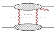
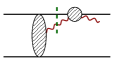
Figure 1: The unitarity cuts associated to the singularities on the physical sheet of the (full-quantum) five-point amplitude, up to permutations. Indeed, we have two unitarity cuts of the first type and four of the second type (which are pushed to infinity in the $q_{i}^{2}$-complex plane in the classical limit). We should emphasise that the first diagram corresponds to singularities which are not in the physical region but can only be probed within complex kinematics: i.e. the graviton propagators should not be thought as delta function, but as residues on their poles (they are commonly referred to as generalised unitarity cuts).

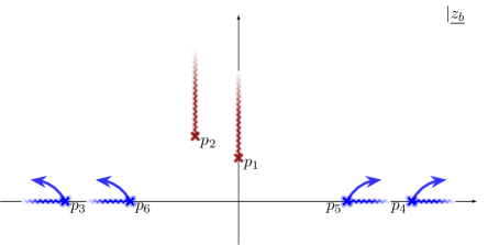
Figure 2: The singularities (poles at tree-level and branch points at loop) of the quantum five-point amplitude. As we take the classical limit (formally, $m_{i}\to+\infty$), the blue singularities – right diagram in Figure 1 – are pushed to infinity and we are left only with the red singularities – left diagram in Figure 1 – in complex kinematics corresponding to $q_{1}^{2}=0$ or $q_{2}^{2}=0$ (even though we are not displaying them, in the $z_{v,q}$ complex plane there are two symmetrical singularities in the lower-half plane). In terms of generalised unitarity cuts, terms which are not probed by the cuts in the $q_{i}^{2}$ channels (but only by Compton-like cuts, on the RHS of Figure 1) do not contribute to the classical waveforms.

3 The soft expansion and the integrand from generalised unitarity

In this section, we are going to present a simplified strategy to construct the integrand for the waveform. It is important to stress that the integrand is in general a function of the loop momentum and the momentum mismatches $q_{i}^{\mu}$, and both such integrations will be discussed in the following section. The two main ingredients discussed in this section are

1. generalised unitarity at the level of the combined FT (18) and the loop integral,

2. the asymptotic expansion in the soft regions of the observable in the classical limit at the level of the generalised unitarity cuts, which was introduced in reference Brandhuber:2021eyq and it is referred to as the heavy-mass expansion.

In particular, generalised unitarity is important to isolate those terms which give non-trivial contributions to the FT. Indeed, we know that the FT is sensitive only to the singularities at $q_{1}^{2}=0$ and $q_{2}^{2}=0$ in the classical limit, while analytic terms would only give localised – short-range – contributions. As mentioned in the previous section, such singularities are probed by the unitarity cuts in Figure 1 (left) and terms which vanish when probing any of these cuts can be discarded.

Then, in this section, we will start computing the Compton amplitude at tree level and one loop and the three-photon amplitude at tree level in the heavy-mass expansion, which appears on the two sides of the $q_{i}^{2}$-cuts. We are going to provide the result in a manifestly gauge-invariant form, similar to Brandhuber:2021kpo . Next, we are going to present an ansatz for the waveform integrand at one-loop and compute it in the case of electrodynamics.

3.1 QED amplitudes in the heavy-mass expansion – Tree-level

We compute the four- and five-point tree-level amplitudes from Feynman diagrams (with $+i\epsilon$ prescription). Before glueing them in the generalised unitarity cuts, we can take the classical limit in the form of the heavy-mass expansion $\bar{m}\gg k_{i},q$ ($q=\sum_{i}^{n}k_{i}$, the incoming massive scalar has momentum $p$ and the outgoing has momentum $p-q$). Here, it is important to emphasise that the heavy-mass expansion has to be taken around the barred variables $\bar{p}$, rather than $p$, as enforced by the on-shell measure (9) (this is important to not miss classical terms from the expansion of the delta function, which would look like $\frac{\hbar}{\hbar}$). The matter-photon coupling is normalised as

$$\mathcal{A}_{3}(p;k)=2e\,\varepsilon_{k}\cdot p\ .$$ (27)

The four-point amplitude in the heavy-mass expansion takes the form

$$\begin{split}\tilde{\mathcal{A}}_{4}^{0}(\bar{m}\bar{u};k_{1},k_{2})&=2ie^{2}\bar{m}\,\hat{\delta}(k_{1}\cdot\bar{u})\,\varepsilon_{1}\cdot\bar{u}\,\varepsilon_{2}\cdot\bar{u}+2e^{2}\frac{\bar{u}\cdot F_{1}\cdot F_{2}\cdot\bar{u}}{k_{1}\cdot\bar{u}^{2}}\\ &+\frac{ie^{2}}{4\bar{m}}\hat{\delta}^{\prime\prime}(k_{1}\cdot\bar{u})\,k_{1}\cdot F_{2}\cdot\bar{u}\,k_{2}\cdot F_{1}\cdot\bar{u}+\mathcal{O}(\bar{m}^{-2})\ .\end{split}$$ (28)

where the dot $\cdot$ stands for a contraction of Lorentz indices, $F_{i}^{\mu\nu}=k_{i}^{\mu}\varepsilon_{i}^{\nu}-k_{i}^{\nu}\varepsilon_{i}^{\mu}$ and we are using the notation

$$\tilde{\mathcal{A}}_{2+n}^{0}(\bar{p};k_{1},\dots,k_{n})=\mathcal{A}_{2+n}^{0}(\bar{p}+\frac{q}{2};k_{1},\dots,k_{n})\ .$$ (29)

The second term in equation (28) is genuinely classical and the linear propagator has to be interpreted with a (symmetric-in-time) principal-value prescription:

$$\frac{1}{x}=\frac{1}{2x+i\epsilon}+\frac{1}{2x-i\epsilon}\ .$$ (30)

Here we have given one additional order to the needed classical expansion for reasons that will be clarified below. The five-point amplitude is

$$\begin{split}\tilde{\mathcal{A}}_{5}^{0}(\bar{p};k_{1},k_{2},k_{3})=&-e^{3}\bar{m}\,\hat{\delta}(k_{1}\cdot\bar{u})\,\hat{\delta}(k_{2}\cdot\bar{u})\,\varepsilon_{1}\cdot\bar{u}\,\varepsilon_{2}\cdot\bar{u}\,\varepsilon_{3}\cdot\bar{u}+\text{perm.'s}\\ &+2ie^{3}\hat{\delta}(k_{1}\cdot\bar{u})\,\varepsilon_{1}\cdot\bar{u}\frac{\bar{u}\cdot F_{2}\cdot F_{3}\cdot\bar{u}}{(k_{2}\cdot\bar{u})^{2}}+\text{perm.'s}\\ &+2e^{3}\frac{q\cdot F_{1}\cdot\bar{u}\,\bar{u}\cdot F_{2}\cdot F_{3}\cdot\bar{u}}{\bar{m}(k_{1}\cdot\bar{u})^{2}\,k_{2}\cdot\bar{u}\,k_{3}\cdot\bar{u}}+\text{perm.'s}+\dots+\mathcal{O}(\bar{m}^{-2})\ ,\end{split}$$ (31)

where the dots stand for additional terms proportional to $\delta(k_{i}\cdot\bar{u})\delta^{\prime\prime}(k_{j}\cdot\bar{u})$, which are irrelevant for the computation of the waveform – to the order considered (for example, such terms are relevant for the computation of the momentum kick at two loops). These terms have not been considered in the original work by Brandhuber et al. Brandhuber:2021kpo and we leave a systematic understanding of these structures for future works, ignoring them in this work as we are genuinely interested in $\omega\neq 0$.

At this point, it is important to understand the tree-level contributions appearing in the KMOC subtractions. We will have the contributions both from factorised four- and five-point amplitudes, which take the form

$$\begin{split}\mathcal{A}_{3}^{0}(p;k_{1})\,\hat{\delta}(2p\cdot k_{1})\,\mathcal{A}_{3}^{0}(p-k_{1};k_{2})&=2e^{2}\bar{m}\,\hat{\delta}(k_{1}\cdot\bar{u})\,\varepsilon_{1}\cdot\bar{u}\,\varepsilon_{2}\cdot\bar{u}\\ &-e^{2}\,\hat{\delta}^{\prime}(k_{1}\cdot\bar{u})\,\bar{u}\cdot F_{1}\cdot F_{2}\cdot\bar{u}+\mathcal{O}(\bar{m}^{-1})\ ,\end{split}$$ (32)

and

$$\begin{split}\mathcal{A}_{4}^{0}(p;k_{1},k_{2})\,\hat{\delta}((p-k_{1}-k_{2})^{2}-m^{2})\,&\mathcal{A}_{3}^{0}(p-k_{1}-k_{2};k_{3})=\dots+2e^{3}\hat{\delta}(k_{3}\cdot\bar{u})\,\varepsilon_{3}\cdot\bar{u}\frac{\bar{u}\cdot F_{1}\cdot F_{2}\cdot\bar{u}}{(k_{1}\cdot\bar{u})^{2}}\\ -&e^{3}\hat{\delta}^{\prime}(\bar{u}\cdot k_{3})\frac{q\cdot F_{3}\cdot\bar{u}\,\bar{u}\cdot F_{1}\cdot F_{2}\cdot\bar{u}}{\bar{m}(k_{1}\cdot\bar{u})^{2}}\\ -&e^{3}\hat{\delta}(\bar{u}\cdot k_{3})\varepsilon_{3}\cdot\bar{u}\frac{q\cdot k_{3}\,\bar{u}\cdot F_{1}\cdot F_{2}\cdot\bar{u}}{\bar{m}(k_{1}\cdot\bar{u})^{3}}\\ -&e^{3}\hat{\delta}(\bar{u}\cdot k_{3})\varepsilon_{3}\cdot\bar{u}\frac{k_{2}\cdot F_{1}\cdot\bar{u}\,k_{3}\cdot F_{2}\cdot\bar{u}}{\bar{m}(k_{1}\cdot\bar{u})^{3}}\\ +&e^{3}\hat{\delta}(\bar{u}\cdot k_{3})\varepsilon_{3}\cdot\bar{u}\frac{k_{3}\cdot F_{1}\cdot\bar{u}\,k_{1}\cdot F_{2}\cdot\bar{u}}{\bar{m}(k_{1}\cdot\bar{u})^{3}}+\mathcal{O}(\bar{m}^{-2})\ ,\end{split}$$ (33)

where we are ignoring again all the terms which have two delta functions. According to equation (16), on the right side we should take the complex conjugate amplitude but, at this order, we have only the three-point coupling and the complex conjugation does not play any role. The factorised five-point amplitude can be easily obtained from the expansion of four-point to sub-classical order (28) (it is manifest that the expansion of the delta mixes different orders in the heavy-mass). This form of the expansion makes it manifest that equation (33) will combine with the five-point (31) to change the $i\epsilon$ prescription of the relevant massive propagator.

3.2 QED amplitudes in the heavy-mass expansion – One-loop

In this section, we compute the full quantum one-loop Compton amplitude using generalised unitarity. First, we probe the singularity in the $(P-k_{1})^{2}$ channel and we get the full amplitude from symmetry. Indeed, in electrodynamics and, in general, in QED without additional matter (or simply in QED at one loop), the discontinuity across the threshold in the $(k_{1}+k_{2})^{2}$ is zero. For example, this is not true in gravity and, when we apply these techniques to the general-relativity waveform, we need to treat such contributions carefully, as we will explain in the following section. For this computation, we need the tree-level four-point amplitude:

$$\mathcal{A}_{4}^{0}(m\,u;k_{1},k_{2})=-8e^{2}\frac{m^{2}\,u\cdot F_{1}\cdot F_{2}\cdot u}{\left(-2mk_{1}\cdot u+i\epsilon\right)\left(2mk_{1}\cdot u-q^{2}+i\epsilon\right)}\ .$$ (34)

The ansatz for the Compton amplitude at one-loop can be written as follows:

$$\begin{split}\mathcal{A}_{4}^{1}(p;k_{1},k_{2})&=d_{\mu\nu}\,j_{1,1,1,1}^{\mu\nu}+d_{\mu}\,j_{1,1,1,1}^{\mu}+d\,j_{1,1,1,1}+c_{\mu}\,j_{1,0,1,1}^{\mu}+c\,j_{1,0,1,1}+b\,j_{1,0,1,0}+\dots\\ &+\tilde{d}_{\mu\nu}\,\tilde{j}_{1,1,1,1}^{\mu\nu}+\tilde{d}_{\mu}\,\tilde{j}_{1,1,1,1}^{\mu}+\tilde{d}\,\tilde{j}_{1,1,1,1}+\tilde{c}_{\mu}\,\tilde{j}_{1,0,1,1}^{\mu}+\tilde{c}\,\tilde{j}_{1,0,1,1}+\tilde{b}\,\tilde{j}_{1,0,1,0}+\dots\ ,\end{split}$$ (35)

where the $b$’s, $c$’s and $d$’s are rational coefficients of the kinematic variables and the (tensor) Feynman integrals are defined as

$$j_{a_{1},a_{2},a_{3},a_{4}}^{\mu_{1}\dots\mu_{n}}=\int\!\hat{\mathrm{d}}^{D}\ell\,\frac{\ell^{\mu_{1}}\,\cdots\,\ell^{\mu_{n}}}{[\ell^{2}]_{+}^{a_{1}}[(p-\ell)^{2}-m^{2}]_{+}^{a_{2}}[(p-k_{1}-\ell)^{2}-m^{2}]_{+}^{a_{3}}[(p-q-\ell)^{2}-m^{2}]_{+}^{a_{4}}}\ ,$$ (36)

with $[p]_{+}=p+i\epsilon$. $\tilde{j}^{\mu_{1}\dots\mu_{n}}_{a_{1},a_{2},a_{3},a_{4}}$ is obtained from the previous equation by symmetry $k_{1}\leftrightarrow k_{2}$. The powers of loop momenta in the numerators come from naïve derivative counting in QED. The loop momenta appearing in the numerator are contracted either with the field strengths or in scalar products which are not in the denominator. The dots in the ansatz (35) stand for integrals which have only transcendental weights carried by the masses, i.e. they are proportional to $(m^{2})^{-\epsilon}$. Such contributions are irrelevant for the classical limit Bini:2021gat and we are going to ignore them.

Now, we can consider the integrand and take the residue in complex kinematics on the 2-torus encircling the poles $\ell^{2}$ and $(p-k_{1}-\ell)^{2}$. Then, we can fix the rational coefficients by matching our ansatz to the product of two tree-level Compton amplitudes, summing over the internal photon states. Since the polarisation vectors appear only inside linearised field strengths, we can use the gauge-invariant identity

$$\sum_{h}F_{k}^{\mu\nu}F_{-k}^{\rho\sigma}=k^{\mu}k^{\rho}\eta^{\nu\sigma}-k^{\nu}k^{\rho}\eta^{\mu\sigma}-k^{\mu}k^{\sigma}\eta^{\nu\rho}+k^{\nu}k^{\sigma}\eta^{\mu\rho}\ .$$ (37)

We find

$$\begin{split}d_{\mu\nu}\ell^{\mu}\ell^{\nu}&=64e^{4}\frac{\ell\cdot F_{1}\cdot p\left[m^{2}\ell\cdot F_{2}\cdot(p-k_{1})+p\cdot k_{1}\,\ell\cdot F_{2}\cdot k_{1}\right]}{(-2p\cdot k_{1})^{2}}\ ,\quad\\ d_{\mu}\ell^{\mu}&=-32e^{4}\frac{\ell\cdot F_{1}\cdot p\ k_{1}\cdot F_{2}\cdot p}{(-2p\cdot k_{1})}\ ,\\ c_{\mu}\ell^{\mu}&=-16e^{4}\frac{p\cdot F_{1}\cdot F_{2}\cdot\ell}{(-2p\cdot k_{1})}\ ,\\ c&=16e^{4}\frac{p\cdot F_{1}\cdot F_{2}\cdot(p-k_{1})}{(-2p\cdot k_{1})}\ ,\\ b&=d=0\ .\end{split}$$ (38)

The remaining coefficients are computed imposing Bose symmetry for the photons. Now, we can consider the classical limit at the level of the integrand. In the heavy-mass expansion, we have

$$\begin{split}d_{\mu\nu}\ell^{\mu}\ell^{\nu}&=64e^{4}\bar{m}^{2}\frac{\ell\cdot F_{1}\cdot\bar{u}\ \ell\cdot F_{2}\cdot\bar{u}}{(-2\bar{u}\cdot k_{1})^{2}}+\mathcal{O}(\bar{m}^{1})\ ,\\ c&=16e^{4}\bar{m}\frac{\bar{u}\cdot F_{1}\cdot F_{2}\cdot\bar{u}}{(-2\bar{u}\cdot k_{1})}+\mathcal{O}(\bar{m}^{0})\ ,\\ \end{split}$$ (39)

and all the other coefficients contributing only to subleading order. Indeed, the Feynman integrals at leading order in the mass expansion look like

$$\begin{split}j_{1,a_{2},1,a_{4}}^{\mu_{1}\dots\mu_{n}}&=\int\!\hat{\mathrm{d}}^{D}\ell\,\frac{\ell^{\mu_{1}}\,\cdots\,\ell^{\mu_{n}}}{[\ell^{2}]_{+}[-2\bar{m}\,\bar{u}\cdot\ell]_{+}^{a_{2}+a_{4}}[-2\bar{m}\,\bar{u}\cdot(\ell+k_{1})]_{+}}+\dots\\ &=\frac{(-1)^{a_{2}+a_{4}}}{(-2\bar{m}\,\bar{u}\cdot k_{1})^{a_{2}+a_{4}}}\int\!\hat{\mathrm{d}}^{D}\ell\,\frac{\ell^{\mu_{1}}\,\cdots\,\ell^{\mu_{n}}}{[\ell^{2}]_{+}[-2\bar{m}\,\bar{u}\cdot(\ell+k_{1})]_{+}}+\dots\ ,\end{split}$$ (40)

where we used partial fractioning and we set to zero the resulting scaleless integrals.

Finally, we notice that the symmetrisation in $k_{1}\leftrightarrow k_{2}$ simply changes the overall sign of $c$, introduces an overall $(-1)^{a_{2}+a_{4}+1}$ in the integrals and modifies the $i\epsilon$ prescription of the massive propagator. The integrals combine to localise the massive propagator on-shell, giving rise to the bubble integrals appearing in the first waveform computations from the heavy-mass approximation Brandhuber:2023hhy ; Herderschee:2023fxh :

$$\tilde{\mathcal{A}}_{4}^{1}(\bar{m}\,\bar{u};k_{1},k_{2})=\frac{d_{\mu\nu}B^{\mu\nu}}{(-2\bar{m}\,\bar{u}\cdot k_{1})^{2}}-\frac{cB}{(-2\bar{m}\,\bar{u}\cdot k_{1})}\ ,$$ (41)

where

$$B^{\mu_{1}\dots\mu_{n}}=-i\int\!\hat{\mathrm{d}}^{D}\ell\,\frac{\ell^{\mu_{1}}\,\cdots\,\ell^{\mu_{n}}}{[\ell^{2}]_{+}}\hat{\delta}(-2\bar{m}\,\bar{u}\cdot(\ell+k_{1}))\ .$$ (42)

We notice that performing the tensor reduction a là Passarino-Veltman the terms proportional to $u^{\mu}$ or $k_{1}^{\mu}$ are projected out by the external kinematics and the term proportional to $\eta^{\mu\nu}$ is the only giving a non-zero contribution. The result is proportional to the tree level.

3.3 Generalised unitarity for the Fourier-loop integrand and tensor reduction

To avoid the appearance of spurious singularities in intermediate steps, we consider the loop integral together with the Fourier integral, and we study it as a genuine 2-loop integral with an exponential factor. In the previous two sections, we have computed the building blocks needed for the construction of the combined Fourier-loop integrand. This means that we supply the usual set of spanning cuts with additional cuts involving single-gravitons exchanges in the $q_{1,2}^{2}$ channels. The simplicity of the problem we are considering allows us to work with unitarity-like cuts, as shown in Figure 3, and avoid larger sets of spanning cuts (for a review on generalised unitarity see e.g. Bern:2011qt ).

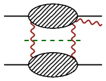
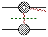
Figure 3: The singularities in the $q_{i}^{2}$ channels are probed by generalised unitarity cuts (in complex kinematics). At one loop we have contributions from the exchange of two gravitons (right) and one graviton (left), with the one-loop Compton amplitude appearing on one side of the cut. In electrodynamics (and, in general, in QED) there is no need for cut merging, which is an analytic procedure to avoid double counting terms which contribute to both.

By inspecting the tree-level amplitudes (or in general the graphs structures and the derivative counting of the Feynman diagrams contributing to the process), we can easily put forward an ansatz for the one-loop waveform:

$$\Delta\langle\mathcal{W}_{h}\rangle=\frac{e^{i\omega\,n\cdot b_{2}}}{4\pi r}\!\int_{\hat{q},\hat{\ell}}\ \hat{\delta}(2\bar{p}_{1}\cdot q)\hat{\delta}(2\bar{p}_{2}\cdot(k-q))\,e^{ib\cdot q}\,\left(\mathcal{I}_{\mathcal{W}}^{D_{1}}+\mathcal{I}^{R_{1}}_{\mathcal{W}}+\mathcal{I}_{\mathcal{W}}^{D_{2}}+\mathcal{I}^{R_{2}}_{\mathcal{W}}\right)\ ,$$ (43)

where

$$\begin{split}\mathcal{I}_{\mathcal{W}}^{D_{1}}&=\sum_{p=0}^{2}\sum_{m+n=0}^{3}D^{(1,p)}_{\mu_{1}\dots\mu_{m},\,\nu_{1}\dots\nu_{n}}\frac{\ell^{\mu_{1}}\cdots\,\ell^{\mu_{m}}q^{\nu_{1}}\cdots\,q^{\nu_{n}}}{\ell^{2}(\ell-q)^{2}(\bar{u}_{2}\cdot\ell)^{p}}(-i)\hat{\delta}(\bar{u}_{1}\cdot\ell)\\ &+\sum_{p=0}^{2}\sum_{m+n=0}^{3}D^{(2,p)}_{\mu_{1}\dots\mu_{m},\,\nu_{1}\dots\nu_{n}}\frac{\ell^{\mu_{1}}\cdots\,\ell^{\mu_{m}}q^{\nu_{1}}\cdots\,q^{\nu_{n}}}{\ell^{2}(\ell-q+k)^{2}(\bar{u}_{2}\cdot\ell)^{p}}(-i)\hat{\delta}(\bar{u}_{1}\cdot\ell)+\dots\end{split}$$ (44)

and

$$\begin{split}\mathcal{I}_{\mathcal{W}}^{R_{1}}=\sum_{m+n=0}^{3}R_{\mu_{1}\dots\mu_{m},\,\nu_{1}\dots\nu_{n}}\frac{\ell^{\mu_{1}}\cdots\,\ell^{\mu_{m}}q^{\nu_{1}}\cdots\,q^{\nu_{n}}}{q^{2}(\ell-q)^{2}}(-i)\hat{\delta}(\bar{u}_{1}\cdot\ell)+\dots\ .\end{split}$$ (45)

The dots stand for terms that do not have a branch point and a pole in $q^{2}=0$ (the numerators cancel either $\ell^{2}$ or $(\ell-q)^{2}$, and $q^{2}$ in the denominator), respectively. This splitting makes sense only in electrodynamics: in gravity or, in general, theories with self-interacting bosons, we will have overlaps between the poles and the branch points in $q_{1,2}^{2}$. This becomes very clear from a quick inspection of the Feynman diagrams in the theory, as shown in Figure 4.

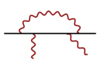
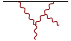
Figure 4: Two of the Feynman diagrams contributing to the one-loop gravitational Compton amplitude. The diagram on the left contributes to the QED amplitude as well, while the one on the right is characteristic of self-interacting bosons. The latter is the origin of the overlap of the poles and discontinuities in the $q_{i}^{2}$ channels.

$\mathcal{I}_{\mathcal{W}}^{D_{2}}$ and $\mathcal{I}_{\mathcal{W}}^{R_{2}}$ are obtained by symmetry, $m_{1}\leftrightarrow m_{2}$, $u_{1}\leftrightarrow u_{2}$, $q\rightarrow k-q$. The computational task is further simplified by noticing that terms which have simultaneous singularities in $q_{1}^{2}$ and $q_{2}^{2}$ do not appear in QED (for example, at tree-level we do not have contributions of the form $\frac{1}{q^{2}(k-q)^{2}}$ and at loop level we do not have pentagons appearing in the ansatz (44)). Then, we can ignore these contributions throughout the computation and obtain the final result (after integration) by symmetrisation $m_{1}\leftrightarrow m_{2}$, $u_{1}\leftrightarrow u_{2}$ and $b_{1}\leftrightarrow b_{2}$. Our results match the integrand of reference Elkhidir:2023dco .

Let us stress an interesting point. The reformulation of generalised unitarity by ansatz makes manifest the fact that the integrand is independent on the $i\epsilon$ prescription (i.e. by the observable we are focusing on), as argued in reference Caron-Huot:2023vxl . Indeed, after writing down an ansatz for the integrand, we probe it by changing the contour of integration to encircle a number of poles of the integrand, putting the corresponding particle on-shell in some complex kinematics – irrespectively of the $i\epsilon$ prescription the original integral had. Perturbative unitarity (at the diagrammatic level) tells us that the corresponding integrand factorises.

The tensor structures appearing in the ansatz (44) and (45) are such that the $\ell$’s and $q$’s are contracted with either the field strengths or with external momenta, such that their scalar product does not appear in the denominators. If we choose to perform tensor reduction at the level of the loop integration only, we would find as an intermediate step a plethora of spurious poles complicating the Fourier integration (even numerically) Brandhuber:2023hhy ; Herderschee:2023fxh ; Bohnenblust:2023qmy . In principle, the amplitude (the Fourier integrand, in general) can be rewritten in terms of a set of functions that are manifestly free of spurious poles on the physical sheet Bini:2024rsy . On the other hand, in this work, we completely bypass this problem, by performing tensor reduction for $\ell$ and $q$ together. Such reduction has been performed using the method proposed in reference Anastasiou:2023koq , which we briefly review in Appendix A. For the sake of our computation, four external vectors appear, which are $b,\bar{u}_{1},\bar{u}_{2},k$ and, in electrodynamics, we encounter tensors up to rank 4.

4 IBP identities for Fourier integrals

In the previous section, we built the integrand of the waveform at one loop via generalized unitarity, and we reduced it to a linear combination of independent tensor structures, multiplied by scalar integrals. In this section, we reduce the number of integrals appearing to a minimal set of linearly independent terms – the MIs – to make the integration problem more accessible. Thus, we introduce integration-by-parts (IBPs) identities for the combined Fourier-loop integrals.

All the scalar integrals appearing belong to the integral family

$$\mathcal{I}_{a_{1},a_{2},a_{3},a_{4},a_{5},a_{6},a_{7},a_{8},a_{9},a_{10},a_{11}}=\int_{\hat{q},\hat{\ell}}\ e^{D_{1}}\prod_{i=1}^{11}\biggl{(}\frac{1}{D_{i}^{a_{i}}}\biggr{)}\ ,$$ (46)

where:

$$D_{1}=iq\cdot b, D_{2}=q^{2}, D_{3}=(q-k)^{2}, D_{4}=\bar{u}_{1}\cdot q, D_{5}=\bar{u}_{2}\cdot(k-q),$$

$$D_{6}=\bar{u}_{1}\cdot\ell D_{7}=\bar{u}_{2}\cdot\ell, D_{8}=\ell^{2}, D_{9}=(\ell+q)^{2}, D_{10}=(\ell+q-k)^{2}, D_{11}=ib\cdot\ell$$ (47)

From the previous section, we know that $b^{\mu}$ can appear only in the numerator as it is produced by tensor reduction. Then, $D_{1,11}$ cannot appear as denominators and $a_{1,11}\leq 0$. Moreover, in the specific case of electrodynamics $D_{2,3}$ never appear together with $D_{9,10}$ as explained in Section 3.3. The on-shell measure forces $D_{4,5}$ to appear as delta functions. But, at the level of IBP relations, this is irrelevant as delta functions can be treated on the same footing as other propagators via reverse unitarity Anastasiou:2002yz ; Anastasiou:2003gr ; Herrmann:2021lqe :

$$\frac{i}{(-1)^{s+1}s!}\hat{\delta}^{(s)}(D_{i})=\frac{1}{(D_{i}+i\epsilon)^{s+1}}-\frac{1}{(D_{i}-i\epsilon)^{s+1}}\ .$$ (48)

Finally, the classical limit localises one matter line per loop (this is manifest in the heavy-mass approach Brandhuber:2021eyq and in the worldline approach Kalin:2020mvi ; Mogull:2020sak ), and we find that either $D_{6}$ or $D_{7}$ are cut. Hence, the scalar integrals can be divided into four families:

$$\mathcal{I}_{a_{1},a_{2},a_{3},1,1,1,a_{7},a_{8},a_{9},a_{10},a_{11}}^{\,\bar{u}_{1}} = \int_{\hat{q},\hat{\ell}}\,e^{D_{1}}\frac{D_{1}^{-a_{1}}D_{2}^{-a_{2}}D_{3}^{-a_{3}}D_{11}^{-a_{11}}\hat{\delta}(D_{4})\hat{\delta}(D_{5})\hat{\delta}(D_{6})}{D_{7}^{a_{7}}D_{8}^{a_{8}}D_{9}^{a_{9}}D_{10}^{a_{10}}}\ ,$$ (49)

$$\mathcal{I}_{a_{1},a_{2},a_{3},1,1,1,a_{7},a_{8},a_{9},a_{10},a_{11}}^{\,\bar{u}_{1},C} = \int_{\hat{q},\hat{\ell}}\,e^{D_{1}}\frac{D_{1}^{-a_{1}}D_{2}^{-a_{2}}D_{7}^{-a_{7}}D_{8}^{-a_{8}}D_{10}^{-a_{10}}D_{11}^{-a_{11}}\hat{\delta}(D_{4})\hat{\delta}(D_{5})\hat{\delta}(D_{6})}{D_{3}^{a_{3}}D_{9}^{a_{9}}}\ ,$$

$\mathcal{I}^{\,\bar{u}_{2}}$ that can be obtained from $\mathcal{I}^{\,\bar{u}_{1}}$ by exchanging $D_{6}\leftrightarrow D_{7}$, and $\mathcal{I}^{\,\bar{u}_{2},C}$ that can be obtained from $\mathcal{I}^{\,\bar{u}_{1},C}$ by exchanging $D_{6}\leftrightarrow D_{7}$, $D_{2}\leftrightarrow D_{3}$, $D_{9}\leftrightarrow D_{10}$.

In dimensional regularisation, IBPs can be performed by imposing that the total derivative w.r.t. the Fourier or the loop momenta vanishes under the integral sign:

$$\int_{\hat{q},\hat{\ell}}\frac{\partial}{\partial{\{\ell^{\mu},q^{\mu}\}}}\biggl{(}\ e^{D_{1}}\frac{v^{\mu}}{\prod_{i=1}^{11}D_{i}^{a_{i}}}\biggr{)}=0$$ (51)

where $v^{\mu}$ can be a linear combination of loop momenta and external momenta. The generation of IBP identities in the presence of exponential functions can be performed algorithmically from the IBP relations generated from the integral family where the exponential is not present. Expanding the total derivative under the integral sign, and recasting the various terms, we have:

$$\int_{\hat{q},\hat{\ell}}e^{D_{1}}\biggl{[}\frac{\partial}{\partial q^{\mu}}\biggl{(}\frac{v^{\mu}}{\prod_{i=1}^{11}D_{i}^{a_{i}}}\biggr{)}+\frac{\partial}{\ \partial{q^{\mu}}}\biggl{(}D_{1}\frac{v^{\mu}}{\prod_{i=1}^{11}D_{i}^{a_{i}}}\biggr{)}-D_{1}\frac{\partial}{\ \partial q^{\mu}}\biggl{(}\frac{v^{\mu}}{\prod_{i=1}^{11}D_{i}^{a_{i}}}\biggr{)}\biggr{]}=0\ .$$ (52)

Equation (52) can be rewritten in terms of standard (two-loop) IBP relations – denoted as IBP$[a_{1},\ldots,a_{11}]$ – of an integral family containing the same set of denominators but not exponentials:

$$\text{IBP}[a_{1},\ldots,a_{11}]+\text{IBP}[a_{1}-1,\ldots,a_{11}]-D_{1}\text{IBP}[a_{1},\ldots,a_{11}]=0\ ,$$ (53)

where we generate $\text{IBP}[a_{1},\ldots,a_{11}]$ using LiteRed Lee:2012cn .

In principle, one can generate and solve the IBP relations in all the sectors appearing. However, it is useful to restrict our attention to the subsets where we expect to find MIs, called non-zero sectors. These can be isolated by counting the number of MIs associated with each sector, as pointed out in references Lee:2013hzt ; Bitoun:2017nre . This counting is most efficiently carried out in Baikov representation Baikov:1996iu ; Frellesvig:2017aai , in which equation (46) is written as a parametric integral over the denominators $z_{i}=D_{i}$:

$$I_{a_{1},\ldots a_{11}}\propto\int\!u(\mathbf{z})\prod_{i=1}^{11}\biggl{(}\frac{dz_{i}}{z_{i}^{a_{i}}}\biggr{)}\ ,\qquad u(\mathbf{z})=\ e^{z_{11}}B(\mathbf{z})^{\gamma}\ ,$$ (54)

where $B(\mathbf{z})=\det\mathbf{G}$ is the Gram determinant of the loop momenta and the external vectors ($q,\ell,u_{1},u_{2},k,b$) and $\gamma=(D-7)/2$. The number of MIs of a given sector $\mathcal{S}$ is obtained as the number of critical points of the regulated function $u_{\mathcal{S}}=u(\mathbf{z})\prod_{i=1}^{11}z_{i}^{\sigma_{i}\rho_{i}}$ Mastrolia:2018uzb ; Frellesvig:2019uqt , where the $\rho_{i}$ are analytic regulators, and it is given as the number of zeroes of

$$\omega_{\mathcal{S}}=\mathrm{d}\log(u_{\mathcal{S}})=\sum_{i=1}^{11}\partial_{z_{i}}(u_{\mathcal{S}})\mathrm{d}z_{i}=0\ .$$ (55)

This computation in practice can be done numerically in Mathematica by solving the system of equations w.r.t. $z_{i}$, or using the Julia package HomotopyContinuation HomotopyContinuation.jl .

Then, restricting to the non-zero sectors, we solved the IBP system twice, using LiteRed Lee:2012cn , and with an in-house routine on FiniteFlow Peraro:2019svx using Laporta method Laporta:2000dsw , finding agreement between the two results. The decomposition in terms of MIs has been independently checked using intersection numbers Mastrolia:2018uzb , using the method developed in Brunello:2023rpq .

Focusing on the relevant sector in equation (49) (with $a_{1,2,3,11}\leq 0$), and in  (LABEL:eq:QED_sector_2) (with $a_{1,3,7,8,10,11}\leq 0$), we find respectively 16 and 2 MIs, but only a subset of them enters the electrodynamics calculation. Moreover, we notice that integrals with different powers of $D_{1}$ in the numerators are related by a differentiation w.r.t. $b^{\mu}$:

$$\mathcal{I}^{\,\bar{u}_{i}}_{-a_{1},a_{2},\ldots,a_{10},0}=\delta_{b}^{(a_{1})}\mathcal{I}^{\,\bar{u}_{i}}_{0,a_{2},\ldots,a_{10},0}\ ,$$ (56)

where

$$\qquad\delta_{b}^{(n)}=b^{\mu_{1}}\cdots b^{\mu_{n}}\frac{\partial}{\partial b^{\mu_{1}}}\cdots\frac{\partial}{\partial b^{\mu_{n}}}\ ,$$ (57)

and we showed for simplicity only the case $a_{11}=0$, which is relevant for our computation.

The one-loop waveform in electrodynamics can be decomposed in terms of ten MIs of the first family:

$$\begin{split}\mathcal{J}^{\,\bar{u}_{1}}_{1+n}&=\mathcal{I}^{\,\bar{u}_{1}}_{-n,0,0,1,1,1,0,1,0,1,0}=\delta_{b}^{(n)}\,\mathcal{F}\left[\parbox[c]{34.6896pt}{\includegraphics[scale={.7}]{figures/triu1}}\right]\ ,\\ \mathcal{J}^{\,\bar{u}_{1}}_{5+m}&=\mathcal{I}^{\,\bar{u}_{1}}_{-m,0,0,1,1,1,1,1,0,1,0}=\delta_{b}^{(m)}\,\mathcal{F}\left[\parbox[c]{34.6896pt}{\includegraphics[scale={.7}]{figures/boxu1}}\right]\ ,\\ \mathcal{J}^{\,\bar{u}_{1}}_{7+m}&=\mathcal{I}^{\,\bar{u}_{1}}_{-m,0,0,1,1,1,0,1,1,0,0}=\delta_{b}^{(m)}\,\mathcal{F}\left[\parbox[c]{34.6896pt}{\includegraphics[scale={.7}]{figures/triu1bl}}\right]\ ,\\ \mathcal{J}^{\,\bar{u}_{1}}_{9+m}&=\mathcal{I}^{\,\bar{u}_{1}}_{-m,0,0,1,1,1,1,1,1,0,0}=\delta_{b}^{(m)}\,\mathcal{F}\left[\parbox[c]{34.6896pt}{\includegraphics[scale={.7}]{figures/boxu1bl}}\right]\ .\end{split}$$ (58)

and two MIs of the second one:

$$\begin{split}\mathcal{J}^{\,\bar{u}_{1},C}_{1+m}&=\mathcal{I}^{\,\bar{u}_{1}}_{-m,0,1,1,1,1,0,0,1,0,0}=\delta_{b}^{(n)}\,\mathcal{F}\left[\parbox[c]{34.6896pt}{\includegraphics[scale={.7}]{figures/compton_mis_v2}}\right]\ ,\end{split}$$ (59)

with $n=0,\dots 3$, $m=0,1$ and $\mathcal{F}$ is a short-hand notation for the FT to impact parameter space:

$$\mathcal{F}[f(q)]=\int_{\hat{q}}e^{iq\cdot b}\,\hat{\delta}(\bar{u}_{1}\cdot q)\,\hat{\delta}(\bar{u}_{2}\cdot(q-k))\,f(q)\ .$$ (60)

Hence, it is sufficient to compute the FT of $\mathcal{J}_{1,5,7,9}^{\,\bar{u}_{1}}$, and of $\mathcal{J}_{1}^{\,\bar{u}_{1},C}$. The final result for the waveform can be written as

$$\Delta\langle\mathcal{W}_{h}\rangle(\omega,\vec{n})=\frac{e^{i\omega\,n\cdot b_{2}}}{4\pi r}\sum_{i=1}^{10}\left(c^{\bar{u}_{1}}_{i}\mathcal{J}^{\,\bar{u}_{1}}_{i}+c^{\bar{u}_{2}}_{i}\mathcal{J}^{\,\bar{u}_{2}}_{i}\ \right)+\frac{e^{i\omega\,n\cdot b_{2}}}{4\pi r}\sum_{i=1}^{2}\left(c^{\bar{u}_{1},C}_{i}\mathcal{J}^{\,\bar{u}_{1},C}_{i}+c^{\bar{u}_{2},C}_{i}\mathcal{J}^{\,\bar{u}_{2},C}_{i}\ \right),$$ (61)

where the coefficients $c^{\bar{u}_{1}}_{i}$ can be found in the ancillary file waveformED.m and $c^{\bar{u}_{2}}_{i}$ are obtained by symmetry.

4.1 Evaluating the Fourier integrals

In Appendix B, we gave the technical details for the evaluation of all the one-loop integrals entering a waveform computation. The relevant one-loop integrals, with retarded (matter) propagators, for the case of electrodynamics are:

$$\begin{split}\parbox[c]{34.6896pt}{\includegraphics[scale={.7}]{figures/compton_mis_v2}}&=-\frac{i\ w_{1}}{4\pi(-q_{2}^{2})}+\mathcal{O}\left(\epsilon^{1}\right),\\ \parbox[c]{34.6896pt}{\includegraphics[scale={.7}]{figures/triu1}}&=\frac{\pi+2i\log\frac{w_{1}+\sqrt{w_{1}^{2}-q_{2}^{2}}}{\sqrt{-q_{2}^{2}}}}{8\pi\sqrt{w_{1}^{2}-q_{2}^{2}}}+\mathcal{O}\left(\epsilon^{1}\right),\\ \parbox[c]{34.6896pt}{\includegraphics[scale={.7}]{figures/triu1bl}}&=\frac{1}{8\sqrt{(-q_{1}^{2})}}+\mathcal{O}\left(\epsilon^{1}\right),\\ \parbox[c]{34.6896pt}{\includegraphics[scale={.7}]{figures/boxu1}}&=\frac{i}{8\pi(-q_{2}^{2})\sqrt{\gamma^{2}-1}}\left(\frac{-q_{2}^{2}}{w_{1}\mu_{\rm IR}}\right)^{-2\epsilon}\left[\frac{1}{\tilde{\epsilon}}-\log\left(\gamma^{2}-1\right)-2\log\left(\gamma+\sqrt{\gamma^{2}-1}\right)+i\pi\right]+\mathcal{O}\left(\epsilon^{1}\right)\\ \parbox[c]{34.6896pt}{\includegraphics[scale={.7}]{figures/boxu1bl}}&=\frac{i}{8\pi(-q_{1}^{2})\sqrt{\gamma^{2}-1}}\left(\frac{-q_{1}^{2}}{w_{2}\mu_{\rm IR}}\right)^{-2\epsilon}\left[\frac{1}{\tilde{\epsilon}}-\log\left(\gamma^{2}-1\right)+i\pi\right]+\mathcal{O}\left(\epsilon^{1}\right),\\ \end{split}$$ (62)

where, we defined $\tilde{\epsilon}=\epsilon\,e^{(\gamma_{E}-\log 4\pi)\epsilon}$, $\gamma_{E}$ is the Euler-Mascheroni constant and $\mu_{\rm IR}$ is the infrared scale introduced in dimensional regularisation. Four of the five integrals appearing in equation (62) can be recast (at least up to corrections of order $\epsilon^{1}$) as

$$\mathcal{F}\left[(-q^{2})^{\alpha}\right]=\frac{\Omega_{D-4}}{\sqrt{\gamma^{2}-1}(2\pi)^{D-2}}\int_{\mathcal{C}}\!\mathrm{d}^{2}z\,z_{v}^{D-4}e^{-iz_{b}\sqrt{-b^{2}}}\,\left(z_{v}^{2}+z_{b}^{2}+\frac{w_{2}^{2}}{\gamma^{2}-1}\right)^{\alpha}\ ,$$ (63)

where $\Omega_{D-4}=\frac{2\pi^{\frac{D-3}{2}}}{\Gamma\left[\frac{D-3}{2}\right]}$ is the “volume” of the $(D-4)$-sphere and $\mathcal{C}$ is the integration contour mentioned above, i.e. $(z_{v},z_{b})\in\mathbb{R}_{+}\times\mathbb{R}$. For the boxes $\mathcal{J}_{5}^{\,\bar{u}_{2}}$ and $\mathcal{J}_{9}^{\,\bar{u}_{1}}$, we have $\alpha=-1-2\epsilon$ – in this case the result is valid only at $\mathcal{O}(\epsilon^{1})$ – while for the triangle $\mathcal{J}_{7}^{\,\bar{u}_{1}}$ we have $\alpha=\frac{D-5}{2}$. The integral is computed in terms of Bessel-$K$ functions:

$$\mathcal{F}\left[(-q^{2})^{\alpha}\right]=-\frac{2}{\sqrt{\gamma^{2}-1}\,(4\pi)^{\frac{D}{2}-1}\,\Gamma(-\alpha)}\left(\frac{2z}{-b^{2}}\right)^{\alpha+\frac{D}{2}-1}K_{\alpha+\frac{D}{2}-1}\left(z\right)\ ,$$ (64)

where we introduced the variable

$$z=\frac{w_{2}\sqrt{-b^{2}}}{\sqrt{\gamma^{2}-1}}\ ,$$ (65)

which scales as $\sim p_{\infty}^{0}$ in the small velocity limit, where $p_{\infty}=\sqrt{\gamma^{2}-1}$ is the expansion parameter Bini:2023fiz . The other triangle is more subtle. It can be expanded in the small velocity limit $p_{\infty}\sim 0$, making each term in the series of the form (64). Then, we find

$$\begin{split}\mathcal{J}_{1}&=\frac{iz}{2(4\pi)^{\frac{3}{2}}\sqrt{-b^{2}\,p_{\infty}}}\sum_{n=0}^{\infty}\left(-\frac{zp_{\infty}}{2}\right)^{n}\left[\frac{K_{n}\left(z\right)}{\Gamma\left[n+\frac{3}{2}\right]}-i\,\frac{K_{n-\frac{1}{2}}\left(z\right)}{\sqrt{\frac{zp_{\infty}}{2}}\,n!}\right]\\ &=\frac{i}{16\pi\sqrt{-b^{2}\,p_{\infty}}}\left\{z\!\int_{0}^{\infty}\!\mathrm{d}x\left[e^{-z\cosh x}\,\mathbf{H}_{-1}\left(z\sqrt{p_{\infty}}\sinh x\right)\right]-i\,\frac{e^{-z\sqrt{1+p_{\infty}}}}{\sqrt{p_{\infty}}}\right\}\ ,\end{split}$$ (66)

where $\mathbf{H}_{\alpha}(z)$ is the Struve function with index $\alpha$. Notice that the integral representation can be efficiently evaluated numerically, as it converges very fast.

5 Conclusions

In this paper, we presented a direct strategy to compute scattering waveforms derived from the KMOC formalism. We clarified the heavy-mass expansion of the tree-level amplitudes, showing that non-trivial contributions containing delta functions can contribute to the classical observables. We exploited the analytic structure of the in-in correlator to single out long-range contributions to the waveform. Moreover, we by-passed the appearance of spurious poles, by performing tensor reduction for combined Fourier-loop tensor structures. Finally, we introduced IBP relations to reduce the number of master integrals, treating the momentum mismatches on the same footing as loop momenta. This strategy allowed us to compute the one-loop waveform in electrodynamics and paves the way for the analytic evaluation of gravitational waveform for arbitrary velocities (within the D’Eath bound DEath:1976bbo ; DiVecchia:2023frv ), which will be presented elsewhere Brunello:toappear .

Our investigation opens the way for a few interesting questions. In the heavy-mass expansion, the structures involving principal-value propagators have been understood in all cases with a single massive source and any number of gluons (or photons, through decoupling identities, or gravitons, through double-copy Bern:2008qj ) Brandhuber:2021kpo ; Brandhuber:2021bsf ; Brandhuber:2022enp . A systematic understanding of classical terms involving delta function contributions is still lacking. Moreover, the computation of the Fourier integrals is performed by computing the loop integrals first (with differential equations or by direct evaluation). The differential equations for the combined Fourier and loop integrals involve integration kernels with Bessel functions with integer and half-integer indices, most probably giving iterated Bessel functions in the $\epsilon$ expansion (for example, see Brunello:2023fef ). At tree level, performing the FT to the time domain simplifies the class of functions appearing Jakobsen:2021lvp (see also Herderschee:2023fxh for a detailed discussion). It will be interesting to investigate whether such simplification holds at loop level as well and if these integrals can be treated on the same footing as ordinary $(L+1)$-loop integrals. Finally, throughout this paper, we have selected terms in the amplitude which have branch points at $q_{i}^{2}$, but we have not computed directly the discontinuity along their branch cuts.

Appendix A Passarino-Veltman reduction

In this appendix, we introduce briefly the Passarino-Veltam reduction a là Anastasiou, Karlen and Vicini Anastasiou:2023koq . The $D$-dimensional space can be decomposed in a physical subspace spanned by a set of $E$ linearly-independent external vectors, $p_{1},\dots,p_{E}$, and an the orthogonal subspace of dimension $D_{\perp}=D-E$. We can write down projectors onto these two subspaces. In particular, the projector onto the physical space is given by

$$\eta_{\parallel}^{\mu\nu}=\sum_{i=1}^{E}p_{i}^{\mu}\langle p_{i}^{\nu}\rangle$$ (67)

where $\langle p_{i}^{\nu}\rangle$ are called dual vectors and are defined such that $p_{i}^{\mu}\langle p_{j,\mu}\rangle=\delta_{ij}$. A closed form of these vectors is given in term of the Gram matrix:

$$\langle p_{i}^{\mu}\rangle=\mathbf{G}^{-1}_{ij}\ p_{j}^{\mu}$$ (68)

where $\mathbf{G}_{ij}=p_{i}\cdot p_{j}$ and $i,j=1,\dots E$. Trivially, the projector onto the orthogonal space is

$$\eta_{\perp}^{\mu\nu}=\eta^{\mu\nu}-\eta_{\parallel}^{\mu\nu}\ .$$ (69)

For a given tensor integral of rank $R$, $I^{\mu_{1}\ldots\mu_{R}}$, its tensor decomposition can be written in closed form as:

$$I^{\mu_{1},\ldots,\mu_{R}}=I_{\nu_{1},\ldots,\nu_{R}}\mathcal{T}\biggl{\{}\prod_{i=1}^{R}\eta_{\parallel}^{\nu_{i}\mu_{i}}\biggr{\}}\ ,$$ (70)

where $\mathcal{T}$ is an ordering symbol, resembling the Wick contractions, defined in reference Anastasiou:2023koq as:

$$\begin{split}\mathcal{T}\biggl{\{}\prod_{i=1}^{R}\eta_{\parallel}^{\nu_{i}\mu_{i}}\biggr{\}}&=\ \ \ \prod_{i=1}^{R}\eta_{\parallel}^{\nu_{i}\mu_{i}}\\ &+\ \wick{\c{\eta}_{\parallel}^{\nu_{1}\mu_{1}}\c{\eta}_{\parallel}^{\nu_{2}\mu_{2}}}\prod_{i=3}^{R}\eta_{\parallel}^{\nu_{i}\mu_{i}}+\text{permutations}\\ &+\ \wick{\c{1}\eta_{\parallel}^{\nu_{1}\mu_{1}}\c{1}\eta_{\parallel}^{\nu_{2}\mu_{2}}\c{2}\eta_{\parallel}^{\nu_{3}\mu_{3}}\c{2}\eta_{\parallel}^{\nu_{4}\mu_{4}}}\prod_{i=5}^{R}\eta_{\parallel}^{\alpha_{i}\mu_{i}}+\text{permutations}+\dots\ ,\end{split}$$ (71)

where the contractions are defined as

$$\prod_{i=1}^{n/2}\wick{\c{\eta}_{\parallel}^{\nu_{i}\mu_{i}}\c{\eta}_{\parallel}^{\nu_{i+1}\mu_{i+1}}}=\prod_{i=1}^{n/2}\eta_{\perp}^{\nu_{i}\nu_{i+1}}\bigl{\langle}\prod_{i=1}^{n/2}\eta_{\perp}^{\mu_{i}\mu_{i+1}}\bigr{\rangle}\ .$$ (72)

Here, $\langle\prod_{i=1}^{n/2}\eta_{\perp}^{\mu_{i}\mu_{i+1}}\bigr{\rangle}$ is the dual of the product of orthogonal projectors, i.e. when contracted with the same number of orthogonal projectors give 1 or 0 if the indices are distributed in the same way or differently, respectively.

We will apply this tensor reduction to the loop momenta and Fourier momentum mismatches. The physical subspace is spanned by the four vectors $b^{\mu}$, $\bar{u}_{1}^{\mu}$, $\bar{u}_{2}^{\mu}$ and $k^{\mu}$. In electrodynamics we encounter tensors reduction up to rank 4.

Appendix B The pentagon integrals from differential equations

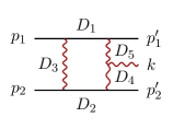
Figure 5: Topology for the one-loop 5-points integrals

The goal of this section is to compute the pentagon integrals appearing in the one-loop amplitude in the heavy-mass limit via differential equations.

All the integrals appearing are related by partial fractioning to the integral family shown in Figure 5:

$$\mathcal{I}_{a1,a2,a3,a4,a5}=e^{\gamma_{E}\epsilon}\int_{\ell}\frac{1}{D_{1}^{a_{1}}D_{2}^{a_{2}}D_{3}^{a_{3}}D_{4}^{a_{4}}D_{5}^{a_{5}}}$$ (73)

where:

$$D_{1}=\bar{u}_{1}\cdot\ell\ , D_{2}=\bar{u}_{2}\cdot\ell, D_{3}=\ell^{2}, D_{4}=(\ell-q_{2})^{2}, D_{5}=(\ell+q_{1})^{2}\ .$$ (74)

In particular, in the heavy-mass expansion, the relevant contributions to the classical limit appear always with either $D_{1}$ or $D_{2}$ localised by a delta function:

$$\mathcal{I}^{\,\bar{u}_{1}}_{1,a_{2},a_{3},a_{4},a_{5}}=e^{\gamma_{E}\epsilon}\int_{\ell}\frac{\hat{\delta}(D_{1})}{D_{2}^{a_{2}}D_{3}^{a_{3}}D_{4}^{a_{4}}D_{5}^{a_{5}}}, \mathcal{I}^{\,\bar{u}_{2}}_{a_{1},a_{2},a_{3},a_{4},a_{5}}=e^{\gamma_{E}\epsilon}\int_{\ell}\frac{\hat{\delta}(D_{2})}{D_{1}^{a_{1}}D_{3}^{a_{3}}D_{4}^{a_{4}}D_{5}^{a_{5}}}$$ (75)

By solving the associated sets of IBPs with LiteRedLee:2012cn , we find that each of the two families has 10 MIs and, since the other can be obtained by symmetries, we can focus on one of them only. We are interested in finding a solution to the associated system of differential equations. It is useful to find a pure basis of integrals Henn:2013pwa , which is a basis in which the $\epsilon$-dependence of the DEs is factorised, and at each order in $\epsilon$ our integrals appear as a sum of uniform-transcendentality functions. A quantity that plays a crucial role in finding a pure basis is the leading singularity (LS) of an integrand, which can be found by replacing the integration paths with contour integrals around the poles of the integrand. At one loop, it is conjectured that an integral with $n$ or $n-1$ legs is pure if it has unit LS in $n$-dimensions Spradlin:2011wp . Moreover, integrals in different space-time dimensions can be related via dimensional-shift identities if their dimension differs by multiples of two Tarasov:1996br ; Lee:2009dh . Hence, we can find a pure basis by rescaling each $n$-point integral by its LS, computed around $d_{0}=n$ (or $n-1$) dimensions, and then relating them to their 4-dimensional representation via dimensional-shift identities. In particular, bubble integrals are pure in $d_{0}=2$, triangles and boxes around $d_{0}=4$, and pentagons around $d_{0}=6$. The LS can be easily computed in Baikov representation, by looking at the maximal cut for each integral Dlapa:2021qsl . Putting everything together we find:

$$\mathcal{G}_{1}\ =\ \frac{\epsilon(1-2\epsilon)}{w_{1}}\ \mathcal{I}^{\,\bar{u}_{1}}_{1,0,0,1,0}\ , \mathcal{G}_{2}\ =\ \epsilon^{2}\sqrt{-q_{1}^{2}}\ \mathcal{I}^{\,\bar{u}_{1}}_{1,0,1,0,1}$$

$$\mathcal{G}_{3}\ =\ \epsilon^{2}\sqrt{w_{1}^{2}-q_{2}^{2}}\ \mathcal{I}^{\,\bar{u}_{1}}_{1,0,1,1,0}\ , \mathcal{G}_{4}\ =\ \epsilon^{2}\sqrt{\gamma^{2}-1}\ \mathcal{I}^{\,\bar{u}_{1}}_{1,1,0,0,1}$$

$$\mathcal{G}_{5}\ =\ \epsilon^{2}\sqrt{\gamma^{2}-1}\ \mathcal{I}^{\,\bar{u}_{1}}_{1,1,0,1,0}\ , \mathcal{G}_{6}\ =\ \epsilon^{2}q_{1}^{2}w_{1}\ \mathcal{I}^{\,\bar{u}_{1}}_{1,0,1,1,1}$$

$$\mathcal{G}_{7}\ =\ \epsilon^{2}w_{1}w_{2}\ \mathcal{I}^{\,\bar{u}_{1}}_{1,1,0,1,1}\ , \mathcal{G}_{8}\ =\ \epsilon^{2}q_{1}^{2}\sqrt{\gamma^{2}-1}\ \mathcal{I}^{\,\bar{u}_{1}}_{1,1,1,0,1}$$

$$\mathcal{G}_{9}\ =\ \epsilon^{2}q_{2}^{2}\sqrt{\gamma^{2}-1}\ \mathcal{I}^{\,\bar{u}_{1}}_{1,1,1,1,0}\ , \mathcal{G}_{10}\ =\ \epsilon^{2}\sqrt{\det\mathbf{G}}\ \mathcal{I}^{\,\bar{u}_{1},6-2\epsilon}_{1,1,1,1,1}$$ (76)

where $\det\mathbf{G}$ is the Gram determinant of the external momenta $\bar{u}_{1,2}$ and $q_{1,2}$.
This basis matches the one obtained in Bohnenblust:2023qmy . Then, one gets a system of DEs in canonical form, which can be combined in a total differential:

$$d\mathcal{G}=\epsilon d\mathbb{A}\mathcal{G}\ ,\qquad d\mathbb{A}=\hat{\mathbb{A}}_{w_{1}}dw_{1}+\hat{\mathbb{A}}_{w_{2}}dw_{2}+\hat{\mathbb{A}}_{-q_{1}^{2}}d(-q_{1}^{2})+\hat{\mathbb{A}}_{-q_{2}^{2}}d(-q_{2}^{2})+\hat{\mathbb{A}}_{\gamma}d\gamma\ ,$$ (77)

where the differential matrix is in $\mathrm{d}\log$ form, and can be written as:

$$d\mathbb{A}=\sum_{i=1}^{42}\mathbb{M}_{i}d\log(\eta_{i})\ .$$ (78)

where: $\eta_{i}$ are called letters, and they contain all the kinematic dependence of the DEs, and $\mathbb{M}_{i}$ are constant matrices. The alphabet consists of 42 letters that can be found using the method developed in Jiang:2024eaj . There are 16 rational letters:

$$\eta_{1}=-q_{1}^{2}, \eta_{2}=-q_{2}^{2}, \eta_{3}=w_{1}, \eta_{4}=w_{2}$$

$$\eta_{5}=\gamma+1, \eta_{6}=\gamma-1, \eta_{7}=q_{1}^{2}-q_{2}^{2}, \eta_{8}=w_{1}^{2}-q_{2}^{2},$$

$$\eta_{9}=w_{2}^{2}-q_{1}^{2}, \eta_{10}=-w_{1}^{2}-w_{2}^{2}+2w_{1}w_{2}\gamma, \eta_{11}=-w_{2}^{2}-q_{1}^{2}(\gamma^{2}-1), \eta_{12}=-w_{1}^{2}-q_{2}^{2}(\gamma^{2}-1)$$

$$\eta_{13}=-4q_{1}^{2}w_{1}^{2}-(q_{1}^{2}-q_{2}^{2})^{2},$$

$$\eta_{14}=-4q_{2}^{2}w_{2}^{2}-(q_{1}^{2}-q_{2}^{2})^{2},$$

$$\eta_{15}=2q_{1}^{2}q_{2}^{2}w_{1}w_{2}\gamma-q_{1}^{4}w_{1}^{2}-q_{2}^{4}w_{2}^{2},$$

$$\eta_{16}=(q_{1}^{2}-q_{2}^{2})^{2}(\gamma^{2}-1)+4(q_{1}^{2}w_{1}(w_{2}\gamma-w_{1})+q_{2}^{2}w_{2}(w_{1}\gamma-w_{2})+w_{1}^{2}w_{2}^{2}),\ \ \ \ \ \ \ \ \ \ \ \ \ \ \ \qquad\ \$$ (79)

and 26 algebraic letters:

$$\eta_{17}=w_{2}+\sqrt{\eta_{9}} \eta_{18}=w_{1}+\sqrt{\eta_{8}}$$

$$\eta_{19}=\gamma+\sqrt{\eta_{5}\eta_{6}} \eta_{20}=-\frac{w_{2}-w_{1}\gamma-w_{1}\sqrt{\eta_{5}\eta_{6}}}{w_{2}-w_{1}\gamma+w_{1}\sqrt{\eta_{5}\eta_{6}}}$$

$$\eta_{21}=-\frac{q_{1}^{2}w_{1}-q_{2}^{2}w_{2}(\gamma-\sqrt{\eta_{5}\eta_{6}})}{q_{1}^{2}w_{1}-q_{2}^{2}w_{2}(\gamma+\sqrt{\eta_{5}\eta_{6}})} \eta_{22}=-\frac{q_{1}^{4}-q_{1}^{2}q_{2}^{2}+2q_{2}^{2}w_{2}(w_{2}-\sqrt{\eta_{9}})}{+q_{1}^{4}-q_{1}^{2}q_{2}^{2}+2q_{2}^{2}w_{2}(w_{2}+\sqrt{\eta_{9}})}$$

$$\eta_{23}=-\frac{q_{2}^{4}-q_{1}^{2}q_{2}^{2}-2q_{1}^{2}w_{1}(w_{1}-\sqrt{\eta_{8}}))}{q_{2}^{4}-q_{1}^{2}q_{2}^{2}-2q_{1}^{2}w_{1}(w_{1}+\sqrt{\eta_{8}})} \eta_{24}=-\frac{w_{1}-\sqrt{\eta_{2}\eta_{5}\eta_{6}}}{w_{1}+\sqrt{\eta_{2}\eta_{5}\eta_{6}}}$$

$$\eta_{25}=-\frac{w_{2}-\sqrt{\eta_{1}\eta_{5}\eta_{6}}}{w_{2}+\sqrt{\eta_{1}\eta_{5}\eta_{6}}} \eta_{26}=-\frac{w_{1}\gamma-\sqrt{\eta_{5}\eta_{6}\eta_{8}}}{w_{1}\gamma+\sqrt{\eta_{5}\eta_{6}\eta_{8}}}$$

$$\eta_{27}=-\frac{w_{2}\gamma-\sqrt{\eta_{5}\eta_{6}\eta_{9}}}{w_{2}\gamma+\sqrt{\eta_{5}\eta_{6}\eta_{9}}} \eta_{28}=\frac{q_{1}^{2}\gamma-\sqrt{\eta_{1}\eta_{9}}}{q_{1}^{2}\gamma+\sqrt{\eta_{1}\eta_{9}}}$$

$$\eta_{29}=\frac{q_{2}^{2}\gamma-\sqrt{\eta_{2}\eta_{8}}}{q_{2}^{2}\gamma+\sqrt{\eta_{2}\eta_{8}}} \eta_{30}=-\frac{q_{1}^{2}+q_{2}^{2}-2\sqrt{\eta_{2}\eta_{9}}}{q_{1}^{2}+q_{2}^{2}+2\sqrt{\eta_{2}\eta_{9}}}$$

$$\eta_{31}=-\frac{q_{1}^{2}+q_{2}^{2}-2\sqrt{\eta_{1}\eta_{8}}}{q_{1}^{2}+q_{2}^{2}+2\sqrt{\eta_{1}\eta_{8}}} \eta_{32}=-\frac{q_{1}^{2}-q_{2}^{2}-2w_{1}\sqrt{\eta_{1}}}{q_{1}^{2}-q_{2}^{2}+2w_{1}\sqrt{\eta_{1}}}$$

$$\eta_{33}=\frac{2w_{1}(w_{2}^{2}-q_{1}^{2})+(q_{1}^{2}+q_{2}^{2})w_{2}\gamma-2\sqrt{\eta_{9}\eta_{16}}}{2w_{1}(w_{2}^{2}-q_{1}^{2})+(q_{1}^{2}+q_{2}^{2})w_{2}\gamma+2\sqrt{\eta_{9}\eta_{16}}} \eta_{34}=\frac{2w_{2}(w_{1}^{2}-q_{2}^{2})+(q_{1}^{2}+q_{2}^{2})w_{1}\gamma-2\sqrt{\eta_{8}\eta_{16}}}{2w_{2}(w_{1}^{2}-q_{2}^{2})+(q_{1}^{2}+q_{2}^{2})w_{1}\gamma+2\sqrt{\eta_{8}\eta_{16}}}$$

$$\eta_{35}=\frac{q_{1}^{2}w_{1}+q_{2}^{2}(w_{1}-2w_{2}\gamma)-2\sqrt{\eta_{2}\eta_{16}}}{q_{1}^{2}w_{1}+q_{2}^{2}(w_{1}-2w_{2}\gamma)+2\sqrt{\eta_{2}\eta_{16}}} \eta_{36}=\frac{q_{2}^{2}w_{2}+q_{1}^{2}(w_{2}-2w_{1}\gamma)-2\sqrt{\eta_{1}\eta_{16}}}{q_{2}^{2}w_{2}+q_{1}^{2}(w_{2}-2w_{1}\gamma)+2\sqrt{\eta_{1}\eta_{16}}}$$ (80)

$$\eta_{37}=\frac{-q_{1}^{2}-q_{2}^{2}+2w_{1}w_{2}\gamma+(q_{1}^{2}+q_{2}^{2})\gamma^{2}-2\sqrt{\eta_{5}\eta_{6}\eta_{16}}}{-q_{1}^{2}-q_{2}^{2}+2w_{1}w_{2}\gamma+(q_{1}^{2}+q_{2}^{2})\gamma^{2}+2\sqrt{\eta_{5}\eta_{6}\eta_{16}}}$$

$$\eta_{38}=\frac{2q_{2}^{2}w_{2}^{2}-q_{1}^{4}(\gamma^{2}-1)+q_{1}^{2}(-2w_{1}w_{2}\gamma+q_{2}^{2}(\gamma^{2}-1))-2q_{1}^{2}\sqrt{\eta_{5}\eta_{6}\eta_{16}}}{2q_{2}^{2}w_{2}^{2}-q_{1}^{4}(\gamma^{2}-1)+q_{1}^{2}(-2w_{1}w_{2}\gamma+q_{2}^{2}(\gamma^{2}-1))+2q_{1}^{2}\sqrt{\eta_{5}\eta_{6}\eta_{16}}}$$

$$\eta_{39}=\frac{-2q_{2}^{2}w_{2}(w_{2}-w_{1}\gamma)-2q_{1}^{2}w_{1}(w_{1}-w_{2}\gamma)+(q_{1}^{2}-q_{2}^{2})^{2}(\gamma^{2}-1)-2(q_{1}^{2}-q_{2}^{2})\sqrt{\eta_{5}\eta_{6}\eta_{16}}}{-2q_{2}^{2}w_{2}(w_{2}-w_{1}\gamma)-2q_{1}^{2}w_{1}(w_{1}-w_{2}\gamma)+(q_{1}^{2}-q_{2}^{2})^{2}(\gamma^{2}-1)+2(q_{1}^{2}-q_{2}^{2})\sqrt{\eta_{5}\eta_{6}\eta_{16}}}$$

$$\eta_{40}=\frac{q_{1}^{2}q_{2}^{2}(w_{2}+w_{1}\gamma)-q_{1}^{2}w_{1}(2w_{1}w_{2}+q_{1}^{2}\gamma)-q_{2}^{4}w_{2}-2q_{1}^{2}w_{1}\sqrt{\eta_{16}}}{q_{1}^{2}q_{2}^{2}(w_{2}+w_{1}\gamma)-q_{1}^{2}w_{1}(2w_{1}w_{2}+q_{1}^{2}\gamma)-q_{2}^{4}w_{2}+2q_{1}^{2}w_{1}\sqrt{\eta_{16}}}$$

$$\eta_{41}=\frac{q_{1}^{2}q_{2}^{2}(w_{2}+w_{1}\gamma)-q_{1}^{2}w_{1}(2w_{1}w_{2}+q_{1}^{2}\gamma)-q_{2}^{4}w_{2}-2q_{2}^{2}w_{2}\sqrt{\eta_{16}}}{q_{1}^{2}q_{2}^{2}(w_{2}+w_{1}\gamma)-q_{1}^{2}w_{1}(2w_{1}w_{2}+q_{1}^{2}\gamma)-q_{2}^{4}w_{2}+2q_{2}^{2}w_{2}\sqrt{\eta_{16}}}$$

$$\eta_{42}=\frac{q_{1}^{2}w_{1}(w_{1}-w_{2}\gamma)+q_{2}^{2}w_{2}(w_{2}-w_{1}\gamma)-2w_{1}^{2}w_{2}^{2}+2w_{1}w_{2}\sqrt{\eta_{16}}}{q_{1}^{2}w_{1}(w_{1}-w_{2}\gamma)+q_{2}^{2}w_{2}(w_{2}-w_{1}\gamma)-2w_{1}^{2}w_{2}^{2}-2w_{1}w_{2}\sqrt{\eta_{16}}}$$ (81)

The system of DEs in $\mathrm{d}\log$ form is provided in the ancillary file dlogDEs.m.
In canonical form we expect only uniform transcendentality functions to appear at each order in $\epsilon$. Following reference Bohnenblust:2023qmy , boundary conditions can be fixed by solving the system of differential equations numerically via AMFlow Liu:2022chg . One can then analytically reconstruct the result order by order in $\epsilon$ via the PSLQ algorithm Duhr:2019tlz , using an ansatz containing at order $n$ all the UT functions of weight $n$. The result for the canonical MIs at $\mathcal{O}\left(\epsilon^{2}\right)$ is:

$$\mathcal{G}_{1} =-\frac{\epsilon}{8\pi}+\frac{\epsilon^{2}}{8\pi}\left[\log\left(\frac{\eta_{3}^{2}}{\pi}\right)-i\pi\right]+\mathcal{O}\left(\epsilon^{3}\right)\ ,$$ (82)

$$\mathcal{G}_{2} =-\frac{i\epsilon^{2}}{16}+\mathcal{O}\left(\epsilon^{3}\right)\ ,$$ (83)

$$\mathcal{G}_{3} =-\frac{\epsilon^{2}}{16\pi}\left[\log\left(\frac{\eta_{2}}{\eta_{18}^{2}}\right)+i\pi\right]+\mathcal{O}\left(\epsilon^{3}\right)\ ,$$ (84)

$$\mathcal{G}_{4} =\frac{\epsilon}{16\pi}+\frac{\epsilon^{2}}{16\pi}\left[\log\left(\frac{4\pi\eta_{5}\eta_{6}}{\eta_{4}^{2}}\right)-i\pi\right]+\mathcal{O}\left(\epsilon^{3}\right)\ ,$$ (85)

$$\mathcal{G}_{5} =\frac{\epsilon}{16\pi}+\frac{\epsilon^{2}}{16\pi}\left[\log\left(\frac{4\pi\eta_{5}\eta_{6}}{\eta_{19}^{2}\eta_{3}^{2}}\right)-i\pi\right]+\mathcal{O}\left(\epsilon^{3}\right)\ ,$$ (86)

$$\mathcal{G}_{6} =\frac{\epsilon}{32\pi}+\frac{\epsilon^{2}}{32\pi}\left[\log\left(\frac{\eta_{2}^{2}\pi}{\eta_{1}^{2}\eta_{3}^{2}}\right)+i\pi\right]+\mathcal{O}\left(\epsilon^{3}\right)\ ,$$ (87)

$$\mathcal{G}_{7} =\frac{\epsilon}{32\pi}+\frac{\epsilon^{2}}{32\pi}\left[\log\left(\frac{\pi}{\eta_{4}^{2}\eta_{19}^{2}}\right)+i\pi\right]+\mathcal{O}\left(\epsilon^{3}\right)\ ,$$ (88)

$$\mathcal{G}_{8} =\frac{\epsilon}{16\pi}+\frac{\epsilon^{2}}{16\pi}\left[\log\left(\frac{4\pi\eta_{4}^{2}}{\eta_{1}^{2}\eta_{5}\eta_{6}}\right)+i\pi\right]+\mathcal{O}\left(\epsilon^{3}\right)\ ,$$ (89)

$$\mathcal{G}_{9} =\frac{\epsilon}{16\pi}+\frac{\epsilon^{2}}{16\pi}\left[\log\left(\frac{4\pi\eta_{3}^{2}}{\eta_{2}^{2}\eta_{5}\eta_{6}\eta_{19}^{2}}\right)+i\pi\right]+\mathcal{O}\left(\epsilon^{3}\right)\ ,$$ (90)

$$\mathcal{G}_{10} =\mathcal{O}\left(\epsilon^{3}\right)\ ,$$ (91)

which agree with the integrals reported in Brandhuber:2023hhy ; Herderschee:2023fxh ; Caron-Huot:2023vxl ; Bohnenblust:2023qmy .

References

- (1) A. Einstein, Über Gravitationswellen, Sitzungsber. Preuss. Akad. Wiss. Berlin (Math. Phys.) 1918 (1918) 154.
- (2) P.C. Peters, Relativistic gravitational bremsstrahlung, Phys. Rev. D 1 (1970) 1559.
- (3) S.J. Kovacs and K.S. Thorne, The Generation of Gravitational Waves. 3. Derivation of Bremsstrahlung Formulas, Astrophys. J. 217 (1977) 252.
- (4) S.J. Kovacs and K.S. Thorne, The Generation of Gravitational Waves. 4. Bremsstrahlung, Astrophys. J. 224 (1978) 62.
- (5) L. Blanchet and T. Damour, Radiative gravitational fields in general relativity I. general structure of the field outside the source, Phil. Trans. Roy. Soc. Lond. A 320 (1986) 379.
- (6) L. Blanchet and T. Damour, Postnewtonian Generation of Gravitational Waves, Ann. Inst. H. Poincare Phys. Theor. 50 (1989) 377.
- (7) L. Blanchet, T. Damour, G. Esposito-Farese and B.R. Iyer, Gravitational radiation from inspiralling compact binaries completed at the third post-Newtonian order, Phys. Rev. Lett. 93 (2004) 091101 [gr-qc/0406012].
- (8) L. Blanchet, G. Faye, Q. Henry, F. Larrouturou and D. Trestini, Gravitational-Wave Phasing of Quasicircular Compact Binary Systems to the Fourth-and-a-Half Post-Newtonian Order, Phys. Rev. Lett. 131 (2023) 121402 [2304.11185].
- (9) L. Blanchet, G. Faye, Q. Henry, F. Larrouturou and D. Trestini, Gravitational-wave flux and quadrupole modes from quasicircular nonspinning compact binaries to the fourth post-Newtonian order, Phys. Rev. D 108 (2023) 064041 [2304.11186].
- (10) D. Bini, T. Damour and A. Geralico, Comparing one-loop gravitational bremsstrahlung amplitudes to the multipolar-post-Minkowskian waveform, Phys. Rev. D 108 (2023) 124052 [2309.14925].
- (11) D. Bini, T. Damour, S. De Angelis, A. Geralico, A. Herderschee, R. Roiban et al., Gravitational Waveform: A Tale of Two Formalisms, 2402.06604.
- (12) W.D. Goldberger and I.Z. Rothstein, An Effective field theory of gravity for extended objects, Phys. Rev. D 73 (2006) 104029 [hep-th/0409156].
- (13) D.A. Kosower, B. Maybee and D. O’Connell, Amplitudes, Observables, and Classical Scattering, JHEP 02 (2019) 137 [1811.10950].
- (14) A. Cristofoli, R. Gonzo, D.A. Kosower and D. O’Connell, Waveforms from amplitudes, Phys. Rev. D 106 (2022) 056007 [2107.10193].
- (15) S. Caron-Huot, M. Giroux, H.S. Hannesdottir and S. Mizera, What can be measured asymptotically?, JHEP 01 (2024) 139 [2308.02125].
- (16) M. Beneke and V.A. Smirnov, Asymptotic expansion of Feynman integrals near threshold, Nucl. Phys. B 522 (1998) 321 [hep-ph/9711391].
- (17) C. Cheung, I.Z. Rothstein and M.P. Solon, From Scattering Amplitudes to Classical Potentials in the Post-Minkowskian Expansion, Phys. Rev. Lett. 121 (2018) 251101 [1808.02489].
- (18) Z. Bern, C. Cheung, R. Roiban, C.-H. Shen, M.P. Solon and M. Zeng, Scattering Amplitudes and the Conservative Hamiltonian for Binary Systems at Third Post-Minkowskian Order, Phys. Rev. Lett. 122 (2019) 201603 [1901.04424].
- (19) Z. Bern, C. Cheung, R. Roiban, C.-H. Shen, M.P. Solon and M. Zeng, Black Hole Binary Dynamics from the Double Copy and Effective Theory, JHEP 10 (2019) 206 [1908.01493].
- (20) A. Brandhuber, G. Chen, G. Travaglini and C. Wen, A new gauge-invariant double copy for heavy-mass effective theory, JHEP 07 (2021) 047 [2104.11206].
- (21) A. Brandhuber, G. Chen, G. Travaglini and C. Wen, Classical gravitational scattering from a gauge-invariant double copy, JHEP 10 (2021) 118 [2108.04216].
- (22) Z. Bern, L.J. Dixon, D.C. Dunbar and D.A. Kosower, One loop n point gauge theory amplitudes, unitarity and collinear limits, Nucl. Phys. B 425 (1994) 217 [hep-ph/9403226].
- (23) Z. Bern, L.J. Dixon, D.C. Dunbar and D.A. Kosower, Fusing gauge theory tree amplitudes into loop amplitudes, Nucl. Phys. B 435 (1995) 59 [hep-ph/9409265].
- (24) Z. Bern and A.G. Morgan, Massive loop amplitudes from unitarity, Nucl. Phys. B 467 (1996) 479 [hep-ph/9511336].
- (25) R. Britto, F. Cachazo and B. Feng, Generalized unitarity and one-loop amplitudes in N=4 super-Yang-Mills, Nucl. Phys. B 725 (2005) 275 [hep-th/0412103].
- (26) R. Britto, E. Buchbinder, F. Cachazo and B. Feng, One-loop amplitudes of gluons in SQCD, Phys. Rev. D 72 (2005) 065012 [hep-ph/0503132].
- (27) R. Britto, B. Feng and P. Mastrolia, The Cut-constructible part of QCD amplitudes, Phys. Rev. D 73 (2006) 105004 [hep-ph/0602178].
- (28) C. Anastasiou, R. Britto, B. Feng, Z. Kunszt and P. Mastrolia, D-dimensional unitarity cut method, Phys. Lett. B 645 (2007) 213 [hep-ph/0609191].
- (29) G. Ossola, C.G. Papadopoulos and R. Pittau, Reducing full one-loop amplitudes to scalar integrals at the integrand level, Nucl. Phys. B 763 (2007) 147 [hep-ph/0609007].
- (30) C. Anastasiou, R. Britto, B. Feng, Z. Kunszt and P. Mastrolia, Unitarity cuts and Reduction to master integrals in d dimensions for one-loop amplitudes, JHEP 03 (2007) 111 [hep-ph/0612277].
- (31) F.V. Tkachov, A theorem on analytical calculability of 4-loop renormalization group functions, Phys. Lett. B 100 (1981) 65.
- (32) K.G. Chetyrkin and F.V. Tkachov, Integration by parts: The algorithm to calculate -functions in 4 loops, Nucl. Phys. B 192 (1981) 159.
- (33) S. Laporta, High-precision calculation of multiloop Feynman integrals by difference equations, Int. J. Mod. Phys. A 15 (2000) 5087 [hep-ph/0102033].
- (34) A.V. Smirnov, Algorithm FIRE – Feynman Integral REduction, JHEP 10 (2008) 107 [0807.3243].
- (35) P. Maierhöfer, J. Usovitsch and P. Uwer, Kira—A Feynman integral reduction program, Comput. Phys. Commun. 230 (2018) 99 [1705.05610].
- (36) R.N. Lee, Presenting LiteRed: a tool for the Loop InTEgrals REDuction, 1212.2685.
- (37) C. Anastasiou and A. Lazopoulos, Automatic integral reduction for higher order perturbative calculations, JHEP 07 (2004) 046 [hep-ph/0404258].
- (38) A. von Manteuffel and C. Studerus, Reduze 2 - Distributed Feynman Integral Reduction, 1201.4330.
- (39) Z. Wu, J. Boehm, R. Ma, H. Xu and Y. Zhang, NeatIBP 1.0, a package generating small-size integration-by-parts relations for Feynman integrals, Comput. Phys. Commun. 295 (2024) 108999 [2305.08783].
- (40) A.V. Kotikov, Differential equations method: New technique for massive Feynman diagrams calculation, Phys. Lett. B 254 (1991) 158.
- (41) E. Remiddi, Differential equations for Feynman graph amplitudes, Nuovo Cim. A 110 (1997) 1435 [hep-th/9711188].
- (42) T. Gehrmann and E. Remiddi, Differential equations for two loop four point functions, Nucl. Phys. B 580 (2000) 485 [hep-ph/9912329].
- (43) M. Argeri and P. Mastrolia, Feynman Diagrams and Differential Equations, Int. J. Mod. Phys. A 22 (2007) 4375 [0707.4037].
- (44) J.M. Henn, Multiloop integrals in dimensional regularization made simple, Phys. Rev. Lett. 110 (2013) 251601 [1304.1806].
- (45) J.M. Henn, Lectures on differential equations for Feynman integrals, J. Phys. A 48 (2015) 153001 [1412.2296].
- (46) M. Argeri, S. Di Vita, P. Mastrolia, E. Mirabella, J. Schlenk, U. Schubert et al., Magnus and Dyson Series for Master Integrals, JHEP 03 (2014) 082 [1401.2979].
- (47) R.N. Lee, Reducing differential equations for multiloop master integrals, JHEP 04 (2015) 108 [1411.0911].
- (48) G.U. Jakobsen, G. Mogull, J. Plefka and J. Steinhoff, Classical Gravitational Bremsstrahlung from a Worldline Quantum Field Theory, Phys. Rev. Lett. 126 (2021) 201103 [2101.12688].
- (49) S. Mougiakakos, M.M. Riva and F. Vernizzi, Gravitational Bremsstrahlung in the post-Minkowskian effective field theory, Phys. Rev. D 104 (2021) 024041 [2102.08339].
- (50) G.U. Jakobsen, G. Mogull, J. Plefka and J. Steinhoff, Gravitational Bremsstrahlung and Hidden Supersymmetry of Spinning Bodies, Phys. Rev. Lett. 128 (2022) 011101 [2106.10256].
- (51) S. De Angelis, R. Gonzo and P.P. Novichkov, Spinning waveforms from KMOC at leading order, 2309.17429.
- (52) A. Brandhuber, G.R. Brown, G. Chen, J. Gowdy and G. Travaglini, Resummed spinning waveforms from five-point amplitudes, JHEP 02 (2024) 026 [2310.04405].
- (53) R. Aoude, K. Haddad, C. Heissenberg and A. Helset, Leading-order gravitational radiation to all spin orders, Phys. Rev. D 109 (2024) 036007 [2310.05832].
- (54) A. Brandhuber, G.R. Brown, G. Chen, S. De Angelis, J. Gowdy and G. Travaglini, One-loop gravitational bremsstrahlung and waveforms from a heavy-mass effective field theory, JHEP 06 (2023) 048 [2303.06111].
- (55) A. Herderschee, R. Roiban and F. Teng, The sub-leading scattering waveform from amplitudes, JHEP 06 (2023) 004 [2303.06112].
- (56) A. Georgoudis, C. Heissenberg and I. Vazquez-Holm, Inelastic exponentiation and classical gravitational scattering at one loop, JHEP 06 (2023) 126 [2303.07006].
- (57) A. Elkhidir, D. O’Connell, M. Sergola and I.A. Vazquez-Holm, Radiation and Reaction at One Loop, 2303.06211.
- (58) L. Bohnenblust, H. Ita, M. Kraus and J. Schlenk, Gravitational Bremsstrahlung in Black-Hole Scattering at : Linear-in-Spin Effects, 2312.14859.
- (59) A. Georgoudis, C. Heissenberg and R. Russo, An eikonal-inspired approach to the gravitational scattering waveform, 2312.07452.
- (60) A. Georgoudis, C. Heissenberg and R. Russo, Post-Newtonian Multipoles from the Next-to-Leading Post-Minkowskian Gravitational Waveform, 2402.06361.
- (61) D.A. Kosower and K.J. Larsen, Maximal Unitarity at Two Loops, Phys. Rev. D 85 (2012) 045017 [1108.1180].
- (62) S. Badger, H. Frellesvig and Y. Zhang, An Integrand Reconstruction Method for Three-Loop Amplitudes, JHEP 08 (2012) 065 [1207.2976].
- (63) P. Mastrolia, E. Mirabella, G. Ossola and T. Peraro, Scattering Amplitudes from Multivariate Polynomial Division, Phys. Lett. B 718 (2012) 173 [1205.7087].
- (64) H. Ita, Two-loop Integrand Decomposition into Master Integrals and Surface Terms, Phys. Rev. D 94 (2016) 116015 [1510.05626].
- (65) J.L. Bourjaily and J. Trnka, Local Integrand Representations of All Two-Loop Amplitudes in Planar SYM, JHEP 08 (2015) 119 [1505.05886].
- (66) P. Mastrolia and S. Mizera, Feynman Integrals and Intersection Theory, JHEP 02 (2019) 139 [1810.03818].
- (67) H. Frellesvig, F. Gasparotto, M.K. Mandal, P. Mastrolia, L. Mattiazzi and S. Mizera, Vector Space of Feynman Integrals and Multivariate Intersection Numbers, Phys. Rev. Lett. 123 (2019) 201602 [1907.02000].
- (68) K. Matsumoto, Intersection numbers for -forms associated with confluent hypergeometric functions, Funkcial. Ekvac. 41 (1998) 291.
- (69) H. Majima, K. Matsumoto and N. Takayama, Quadratic relations for confluent hypergeometric functions, Tohoku Math. J. (2) 52 (2000) 489.
- (70) S.L. Cacciatori and P. Mastrolia, Intersection Numbers in Quantum Mechanics and Field Theory, 2211.03729.
- (71) G. Brunello, G. Crisanti, M. Giroux, P. Mastrolia and S. Smith, Fourier Calculus from Intersection Theory, 2311.14432.
- (72) G. Brunello and S. De Angelis, to appear, 24xx.xxxxx.
- (73) S. Caron-Huot, M. Giroux, H.S. Hannesdottir and S. Mizera, Crossing beyond scattering amplitudes, 2310.12199.
- (74) E. Herrmann, J. Parra-Martinez, M.S. Ruf and M. Zeng, Radiative classical gravitational observables at (G3) from scattering amplitudes, JHEP 10 (2021) 148 [2104.03957].
- (75) E.H. Wichmann and J.H. Crichton, Cluster Decomposition Properties of the Matrix, Phys. Rev. 132 (1963) 2788.
- (76) S. Weinberg, The Quantum theory of fields. Vol. 1: Foundations, Cambridge University Press (6, 2005), 10.1017/CBO9781139644167.
- (77) G. Passarino and M.J.G. Veltman, One Loop Corrections for e+ e- Annihilation Into mu+ mu- in the Weinberg Model, Nucl. Phys. B 160 (1979) 151.
- (78) K.T.R. Davies, M.L. Glasser, V. Protopopescu and F. Tabakin, The Mathematics of Principal Value Integrals and Applications to Nuclear Physics, Transport Theory, and Condensed Matter Physics, Math. Models Methods Appl. Sci. 06 (1996) 833.
- (79) D. Bini, T. Damour and A. Geralico, Radiative contributions to gravitational scattering, Phys. Rev. D 104 (2021) 084031 [2107.08896].
- (80) Z. Bern and Y.-t. Huang, Basics of Generalized Unitarity, J. Phys. A 44 (2011) 454003 [1103.1869].
- (81) C. Anastasiou, J. Karlen and M. Vicini, Tensor reduction of loop integrals, 2308.14701.
- (82) C. Anastasiou and K. Melnikov, Higgs boson production at hadron colliders in NNLO QCD, Nucl. Phys. B 646 (2002) 220 [hep-ph/0207004].
- (83) C. Anastasiou, K. Melnikov and F. Petriello, A new method for real radiation at NNLO, Phys. Rev. D 69 (2004) 076010 [hep-ph/0311311].
- (84) E. Herrmann, J. Parra-Martinez, M.S. Ruf and M. Zeng, Gravitational Bremsstrahlung from Reverse Unitarity, Phys. Rev. Lett. 126 (2021) 201602 [2101.07255].
- (85) G. Kälin and R.A. Porto, Post-Minkowskian Effective Field Theory for Conservative Binary Dynamics, JHEP 11 (2020) 106 [2006.01184].
- (86) G. Mogull, J. Plefka and J. Steinhoff, Classical black hole scattering from a worldline quantum field theory, JHEP 02 (2021) 048 [2010.02865].
- (87) R.N. Lee and A.A. Pomeransky, Critical points and number of master integrals, JHEP 11 (2013) 165 [1308.6676].
- (88) T. Bitoun, C. Bogner, R.P. Klausen and E. Panzer, Feynman integral relations from parametric annihilators, Lett. Math. Phys. 109 (2019) 497 [1712.09215].
- (89) P.A. Baikov, Explicit solutions of the multiloop integral recurrence relations and its application, Nucl. Instrum. Meth. A 389 (1997) 347 [hep-ph/9611449].
- (90) H. Frellesvig and C.G. Papadopoulos, Cuts of Feynman Integrals in Baikov representation, JHEP 04 (2017) 083 [1701.07356].
- (91) P. Breiding and S. Timme, HomotopyContinuation.jl: A Package for Homotopy Continuation in Julia, in International Congress on Mathematical Software, pp. 458–465, Springer, 2018.
- (92) T. Peraro, FiniteFlow: multivariate functional reconstruction using finite fields and dataflow graphs, JHEP 07 (2019) 031 [1905.08019].
- (93) G. Brunello, V. Chestnov, G. Crisanti, H. Frellesvig, M.K. Mandal and P. Mastrolia, Intersection Numbers, Polynomial Division and Relative Cohomology, 2401.01897.
- (94) P.D. D’Eath, High Speed Black Hole Encounters and Gravitational Radiation, Phys. Rev. D 18 (1978) 990.
- (95) P. Di Vecchia, C. Heissenberg, R. Russo and G. Veneziano, The gravitational eikonal: from particle, string and brane collisions to black-hole encounters, 2306.16488.
- (96) Z. Bern, J.J.M. Carrasco and H. Johansson, New Relations for Gauge-Theory Amplitudes, Phys. Rev. D 78 (2008) 085011 [0805.3993].
- (97) A. Brandhuber, G. Chen, H. Johansson, G. Travaglini and C. Wen, Kinematic Hopf Algebra for Bern-Carrasco-Johansson Numerators in Heavy-Mass Effective Field Theory and Yang-Mills Theory, Phys. Rev. Lett. 128 (2022) 121601 [2111.15649].
- (98) A. Brandhuber, G.R. Brown, G. Chen, J. Gowdy, G. Travaglini and C. Wen, Amplitudes, Hopf algebras and the colour-kinematics duality, JHEP 12 (2022) 101 [2208.05886].
- (99) M. Spradlin and A. Volovich, Symbols of One-Loop Integrals From Mixed Tate Motives, JHEP 11 (2011) 084 [1105.2024].
- (100) O.V. Tarasov, Connection between Feynman integrals having different values of the space-time dimension, Phys. Rev. D 54 (1996) 6479 [hep-th/9606018].
- (101) R.N. Lee, Space-time dimensionality D as complex variable: Calculating loop integrals using dimensional recurrence relation and analytical properties with respect to D, Nucl. Phys. B 830 (2010) 474 [0911.0252].
- (102) C. Dlapa, X. Li and Y. Zhang, Leading singularities in Baikov representation and Feynman integrals with uniform transcendental weight, JHEP 07 (2021) 227 [2103.04638].
- (103) X. Jiang, J. Liu, X. Xu and L.L. Yang, Symbol letters of Feynman integrals from Gram determinants, 2401.07632.
- (104) X. Liu and Y.-Q. Ma, AMFlow: A Mathematica package for Feynman integrals computation via auxiliary mass flow, Comput. Phys. Commun. 283 (2023) 108565 [2201.11669].
- (105) C. Duhr and F. Dulat, PolyLogTools — polylogs for the masses, JHEP 08 (2019) 135 [1904.07279].