Overlapping community detection algorithms using Modularity and the cosine

Abstract

The issue of network community detection has been extensively studied across many fields. Most community detection methods assume that nodes belong to only one community. However, in many cases, nodes can belong to multiple communities simultaneously.This paper presents two overlapping network community detection algorithms that build on the two-step approach, using the extended modularity and cosine function. The applicability of our algorithms extends to both undirected and directed graph structures. To demonstrate the feasibility and effectiveness of these algorithms, we conducted experiments using real data.

Email: ddhieu@math.ac.vn (Do Duy Hieu), phanhaduong@math.ac.vn (Phan Thi Ha Duong).

1 Introduction

In recent years, many studies have focused on network systems such as social networks, biological networks, and technological networks [30, 4]. One of the focal issues of those studies is about the community detection problem [14, 15, 22, 40].

Actually the majority of methods assume that nodes belong to only one community, however in many cases, nodes can participate in multiple communities simultaneously, making the problem more challenging. Some authors have made significant efforts to characterize communities with overlapping nodes, as evidenced by recent papers such as [35, 36, 23, 21]. Nevertheless truly effective algorithms remain a subject requiring further research and demanding new methods.

1.1 Overlapping community detection algorithms

We employ the concept of constructing overlapping communities in two steps: the first step involves using an algorithm to partition the graph into disjoint communities, while the second step entails examining which communities each vertex can potentially belong to.

We are interested in two following algorithms.

First, we are interested in the algorithm introduced in [37], and temporarily call it Parameterized Overlap Algorithm (or Paramet. Overlap for short). For this algorithm, the authors propose a simple approach to identify overlapping communities in a graph $G=(V,E)$, where $V=\{v_{1},v_{2},...,v_{n}\}$ represents $n$ nodes and $E\subseteq V\times V$ represents $m$ edges. Let $C=\{C_{1};C_{2};...;C_{k}\}$ be a family of subsets of nodes (called also cluster or community) that covers $V$. One then decides a vertex $v$ will be added in a cluster $C_{j}$ if their belonging coefficient $F_{vc}$ is greater than or equal to a given threshold parameter $\theta$. The belonging coefficients is defined as follows.

$$F_{vC_{j}}=\begin{cases}1\,\,\,\,if\,\frac{\sum_{(v,u)\in E}\chi_{uC_{j}}}{d_{v}}\geq\theta,\\ 0\,\,\,\,otherwise.\end{cases}$$ (1.1)

where $\chi_{uC_{j}}$ is equal to $1$ if $u\in C_{j}$ and $0$ otherwise and $d_{v}$ is the degree of vertex $v$.

Thus, the belonging coefficient $F_{vC_{j}}$ is proportional to the number of adjacent edges of $v$ belonging to the cluster $C_{j}$. As the value of $\theta$ increases, the degree of overlapping between the communities also increases.

The second algorithm was introduced in [10]. We temporarily call this Module Overlap Algorithm because the main idea of this algorithm is based on the objective of increasing the modularity $Q_{0}$ step by step. For instance, the Modularity $Q_{0}$ for the overlapping community is defined as follows:

$$Q_{0}=\frac{1}{2m}\sum_{C_{j}\in C}\sum_{u,v\in V}\alpha_{uC_{j}}\alpha_{vC_{j}}\left(A_{uv}-\frac{d_{u}d_{v}}{2m}\right),$$

where

$$\alpha_{uC_{j}}=\frac{d_{uC_{j}}}{\sum_{C_{j}\in C}d_{uC_{j}}},\mbox{ with }d_{uC_{j}}=\Sigma_{v\in C_{j}}A_{uv}.$$ (1.2)

1.2 Random walk on graphs

Let $G=(V,E)$ be a directed graph with $n$ vertices and $m$ edges, define $A$ the adjacency matrix of $G$. For $i=1,2,...,n$, we define $d^{out}_{i}$ the out-degree of vertex $i$, and $d^{in}_{i}$ the in-degree of vertex $i$.

It is worth noting that undirected graphs can be seen as a special case of directed graphs, where the adjacency matrix is symmetric and the out-degree and in-degree of each vertex are equal.

For conciseness, in the following, we will use the out-degree of a vertex as its degree, denoted by $d_{i}$ unless stated otherwise.

A random walk on $G$ is a process that starts at a given vertex and moves to another vertex at each time step, the next vertex in the walk is chosen uniformly at random from among the neighbors of the current vertex. The matrix $P=[p_{ij}]_{i,j=\overline{1,n}}$ represents the transition probabilities of a Markov chain associated with a random walk on graph $G$. At each vertex $i$, the random walk can move to vertex $j$ with probability $p_{ij}=a_{ij}/d_{i}$ if $(i,j)\in E$. Then $P=D^{-1}A$ where $D$ being the diagonal matrix $D$ using the vertex out-degrees. Moreover $P^{t}$ represents the transition probabilities of this random walk after $t$ steps.

We assume that $G$ is strongly connected, meaning there is a directed path from any vertex $i$ to every other vertex $j$. According to the convergence theorem for finite Markov chains, the associated transition matrix $P$ satisfies $\lim_{k\rightarrow\infty}P=P_{\infty}$, where $(P_{\infty})_{ij}=\phi_{j}$, the $j$ th component of the unique stationary distribution $\phi=(\phi_{1},\phi_{2},...,\phi_{n})$.

For an undirected graph $G$ where $a_{ij}=a_{ji}$, we have $d_{i}=d^{out}_{i}=d^{in}_{i}$, and $\phi_{i}=d_{i}/2m$ for all vertex $i$.

1.3 Our contribution

In this paper, each algorithm consists of two steps. In the first step, we use existing community detection algorithms, such as the Hitting times Walktrap algorithm [11], Walktrap algorithm [34], or the Louvain algorithm [37], to find disjointed communities for the network. In the second step, we determine whether a vertex belongs to a community or not by using modularity or cosine functions.

• In Section 2, we introduce a concept called Theta-Modularity, an extension of regular Modularity. The criteria for a vertex to belong to a community is that the number of edges between them must be sufficiently large and dependent on the total degree of the vertices in that community.

• In Section 3, we identify each vertex as a vector and define the center of a cluster to be the vertex corresponding to the vector the average coordinates of the vertices in that cluster. Finally, we will propose an overlapping algorithm based on the idea that vertices of the same cluster will create a small angle with the cluster center; in other words, the cosine of that vertex and the cluster center are more significant than a constant $\theta$.

Finally, to assess the effectiveness and rationality of our algorithms, we will conduct experiments to compare and evaluate the clustering results of our algorithms with other algorithms Specifically, in Subsection 5.2.2, we will compare two of our algorithms for undirected graphs, namely the Parameterized Modularity Overlap Algorithm and the Cosine Overlap Algorithm, with two other algorithms Parameterized Overlap Algorithm [37] and the Module Overlap Algorithm [10]. Additionally, we will perform experiments on real datasets and compare the algorithms based on Modularity. In Subsection 5.2.3, we will apply our directed graph algorithms to randomly generated graphs and compare the results with the clustering generated by the graph generation model.

2 Overlapping community detection using modularity

In this section, we will use the modularity function to determine whether a vertex belongs to a community or not. The classic modularity function evaluates the difference between the real number of edges between two vertices and the expected number of edges between them. Our new approach is to introduce a threshold for the expected number of edges in order to make the evaluation more flexible. This new parameterized modularity function will be applied to undirected graphs in section 2.1, and to directed graphs in section 2.2 where the expected number is calculated based on the degree of the vertices. A breakthrough in section 2.3 is that the parameterized modularity function for directed graphs will be defined based on the stationary distribution of a random walk on the graph. This provides a more advanced approach to determining community membership.

2.1 Overlapping community detection for undirected graphs

The expected number of edges falling between two vertices $u$ and $v$ in the configuration model is equal to $d_{u}d_{v}/2m$, then the actual-minus-expected edge count for the vertex pair $(u,v)$ is $A_{uv}-d_{u}d_{v}/2m$. Suppose $C=\{C_{1},C_{2},...,C_{k}\}$ is a cover of the vertices of the undirected graph $G$, the modularity $Q$ (as defined in [29]) is then equal to

$$Q=\frac{1}{2m}\sum_{u,v\in V}\left(A_{uv}-\frac{d_{u}d_{v}}{2m}\right)\delta\left(C_{u},C_{v}\right)\\ =\frac{1}{2m}\sum_{C_{j}\in C}\sum_{u,v\in C_{j}}\left(A_{uv}-\frac{d_{u}d_{v}}{2m}\right).$$ (2.1)

where $\delta\left(C_{u},C_{v}\right)$ is $1$ if $u$ and $v$ are in the same community, and $0$ otherwise.

This modularity illustrates the criteria that $u$ and $v$ belong to the same cluster if the real number of edges between them is greater than the expected number of edges between them. However, we find many practical problems when dividing clusters by data, depending on the goal the required criteria is more flexible. Therefore, we propose a new modularity with theta coefficient as follows.

$$Q(\theta)=\frac{1}{2m}\sum_{C_{j}\in C}\sum_{u,v\in C_{j}}\left(A_{uv}-\theta\frac{d_{u}d_{v}}{2m}\right).$$ (2.2)

Thís new modularity means that two vertices $u$ and $v$ belong to the same cluster if the number of edges between $u$ and $v$ is more significant than $\theta$-times the expected number of edges between them.

We observe that the modularity of clustering of graph $G$ can be expressed as the sum of the modularity of each cluster, as shown in formula 2.2. This implies that if we add a vertex to a cluster, only the modularity value of that specific cluster will be affected. As a result, for every community $C_{j}$ and vertex $u\in V(G)\setminus C_{j}$, the modularity of cluster $C_{j}$ will change by an amount when we add vertex $u$ to it, and the following formula can calculate it.

$$\Delta Q(\theta)_{u,C_{j}}=\dfrac{1}{2m}\sum_{w\in C_{j}}\left(A_{uw}-\theta\dfrac{d_{u}d_{w}}{2m}\right).$$ (2.3)

From the above comment, we propose that vertex $u$ will be added to the community $C_{j}$ if $\Delta Q(\theta)_{u,C_{j}}$ is positive:

$$\dfrac{1}{2m}\sum_{w\in C_{j}}\left(A_{uw}-\theta\dfrac{d_{u}d_{w}}{2m}\right)>0,$$ (2.4)

which corresponds to

$$\sum_{w\in C_{j}}\frac{A_{uw}}{d_{u}}>\theta\sum_{w\in C_{j}}\dfrac{d_{w}}{d}.$$ (2.5)

Remark 2.1

From (1.1) and (2.5), we have remarked that vertex $u$ belongs to the community $C_{j}$ if the number of edges between $u$ and $C_{j}$ is large enough. However, in the equation (1.1), the number of edges between $u$ and $C_{j}$ must always be greater than a fixed $\theta$ constant. It is independent of the properties of the community $C_{j}$. Our method is more reasonable because it depends not only on the $\theta$ coefficient but also on the characteristics of the community $C_{j}$. Specifically, it depends on the sum of the degrees of the vertices in the community $C_{j}$.

From there, we propose the overlap detection algorithm described in Algorithm 1. We will call this the Parameterized Modularity Overlap Algorithm for undirected graphs (or Paramet. Modul. for short).

Input: An undirected graph $G$ and a threshold value $\theta$

Output: Clusters of vertices with overlapping communities

Apply the Louvain algorithm [42] to obtain the initial clustering of $G$ into communities $C_{1},C_{2},...,C_{k}$;

repeat

       foreach vertex $u$ do

             foreach community $C_{j}$ adjacent to $u$ and not containing $u$ do

                   if $\sum_{w\in C_{j}}\frac{A_{uw}}{d_{u}}>\theta\sum_{w\in C_{j}}\dfrac{d_{w}}{d}$ then

                         Add $u$ to $C_{j}$;

                        

                   end if

                  

             end foreach

            

       end foreach

      

until No communities $C_{j}$ meet the condition;

Algorithm 1 Parameterized Modularity Overlap Algorithm

In the Algorithm 1, we have to traverse all the vertices, and for each vertex, we consider all the adjacent communities with it. So the computational complexity of this Algorithm will be $O(kn)$, where $n$ is the number of vertices of the graph, and $k$ is the number of communities.

2.2 Overlapping community detection for directed graphs using modularity

In [2, 27], the authors had given the in/out-degree sequence of directed graph, in which the probability to have an edge from vertex $v$ to vertex $u$ is determined by $d^{in}_{u}d^{out}_{v}$, where $d^{in}_{u}$ and $d^{out}_{v}$ are the in- and out-degrees of the vertices. Suppose $C=\{C_{1},C_{2},...,C_{k}\}$ is a cover of $G$, the modularity $Q$ is defined as.

$$Q^{d}=\frac{1}{m}\sum_{C_{j}\in C}\sum_{u,v\in C_{j}}\left(A_{uv}-\dfrac{d^{in}_{u}d^{out}_{v}}{m}\right),$$ (2.6)

where $A_{uv}$ is defined conventionally to be $1$ if there is an edge from $v$ to $u$ and zero otherwise. Note that indeed edges $v\rightarrow u$ make larger contributions to this expression if $d^{in}_{u}$ and/or $d^{out}_{v}$ is small.

Similar to the case of undirected graphs, we also define Theta-Modularity as follows:

$$Q^{d}(\theta)=\frac{1}{m}\sum_{C_{j}\in C}\sum_{u,v\in C_{j}}\left(A_{uv}-\theta\dfrac{d^{in}_{u}d^{out}_{v}}{m}\right).$$ (2.7)

Then for each community $C_{j}$, we will consider the vertices $u\in V(G)\setminus C_{j}$. We notice that if a vertex $u$ added to the community $C_{j}$, the modulus of the cluster $C_{j}$ changes by an amount of

$$\Delta Q^{d}(\theta)_{u,C_{j}}=\frac{1}{m}\sum_{w\in C_{j}}\left(A_{uw}-\theta\dfrac{d^{in}_{u}d^{out}_{w}}{m}\right)+\frac{1}{m}\sum_{w\in C_{j}}\left(A_{wu}-\theta\dfrac{d^{in}_{w}d^{out}_{u}}{m}\right).$$ (2.8)

From the above comment, we propose that vertex $u$ belongs to the community $C_{j}$ if $\Delta Q^{d}(\theta)_{u,C_{j}}$ is positive:

$$\frac{1}{m}\sum_{w\in C_{j}}\left(A_{uw}-\theta\dfrac{d^{in}_{u}d^{out}_{w}}{m}\right)+\frac{1}{m}\sum_{w\in C_{j}}\left(A_{wu}-\theta\dfrac{d^{in}_{w}d^{out}_{u}}{m}\right)>0.$$ (2.9)

equivalent to

$$\sum_{w\in C_{j}}\left(A_{uw}+A_{wu}\right)>\theta\sum_{w\in C_{j}}\left(\dfrac{d^{in}_{u}d^{out}_{w}}{m}+\dfrac{d^{in}_{w}d^{out}_{u}}{m}\right),$$ (2.10)

Remark 2.2

From (2.10), we have remarked that vertex $u$ belongs to the community $C_{j}$ if the total number of edges from $u$ to $C_{j}$ and the number of edges from $C_{j}$ to $u$ is large enough.

From there, we propose the overlap detection algorithm described in Algorithm 2. We will call this the Directed Parameterized d-Modularity Overlap Algorithm for directed graphs (or Di-Paramet. d-Modul. for short)

Input: A directed graph $G$ and a threshold value $\theta$

Output: Clusters of vertices with overlapping communities

Apply Louvain algorithm [12] to obtain the initial clustering of $G$ into communities $C_{1},C_{2},...,C_{k}$;

repeat

       foreach vertex $u$ do

             foreach community $C_{j}$ adjacent to $u$ and not containing $u$ do

                   if $\sum_{w\in C_{j}}\left(A_{uw}+A_{wu}\right)>\theta\sum_{w\in C_{j}}\left(\dfrac{d^{in}_{u}d^{out}_{w}}{m}+\dfrac{d^{in}_{w}d^{out}_{u}}{m}\right)$ then

                         Add $u$ to $C_{j}$;

                        

                   end if

                  

             end foreach

            

       end foreach

      

until No communities $C_{j}$ meet the condition;

Algorithm 2 Directed Parameterized d-Modularity Overlap Algorithm

Similar to the Algorithm 1, the Algorithm 2 also has a computational complexity of $O(kn)$, where $n$ is the number of vertices of the graph, and $k$ is the number of communities.

2.3 Overlapping community detection for directed graphs using the stationary distribution

Many modularities have been proposed for directed graphs, such as the Modularity in Formula 2.6. In many cases, those modularity proposals will lose the essential properties of directed graphs. Therefore, in [11], we proposed a definition of modularity for directed graphs based on random walks and stationary distribution, which is a natural extension of modularity on undirected graphs. In detail, for a cover $C=\{C_{1},C_{2},...,C_{k}\}$ of the directed graph $G$, our proposed modularity is the following.

$$Q^{sd}=\sum_{uv}\left(P_{vu}\phi_{v}-\phi_{u}\phi_{v}\right)\delta_{C_{u}C_{v}},$$ (2.11)

where $P_{vu}$ is the transition probability of the random walk process from $v$-th vertex to $u$-th vertex and $\phi=\left(\phi_{1},\phi_{2},...,\phi_{n}\right)$ is the stationary distribution stationary.

We also have the $\theta$ modularity version as follows.

$$Q^{sd}(\theta)=\sum_{uv}\left(P_{vu}\phi_{v}-\theta\phi_{u}\phi_{v}\right)\delta_{C_{u}C_{v}}.$$ (2.12)

and then

$$Q^{sd}(\theta)=\sum_{C_{j}\in C}\sum_{u,v\in C_{j}}\left(P_{vu}\phi_{v}-\theta\phi_{u}\phi_{v}\right).$$ (2.13)

Then for each community $C_{j}$, we will consider the vertices $u\in V(G)\setminus C_{j}$: if $u$ is added to the community $C_{j}$ the modularity of the cluster $C_{j}$ changes by an amount of

$$\Delta Q^{sd}(\theta)_{u,C_{j}}=\sum_{w\in C_{j}}\left(\phi_{u}P_{uw}-\theta\phi_{u}\phi_{w}\right)+\sum_{w\in C_{j}}\left(\phi_{w}P_{wu}-\theta\phi_{u}\phi_{w}\right).$$ (2.14)

We also propose that vertex $u$ belongs to community $C_{j}$ if $\Delta Q^{sd}(\theta)_{u,C_{j}}$ is positive, that means:

$$\sum_{w\in C_{j}}\left(\phi_{u}P_{uw}-\theta\phi_{u}\phi_{w}\right)+\sum_{w\in C_{j}}\left(\phi_{w}P_{wu}-\theta\phi_{u}\phi_{w}\right)>0,$$ (2.15)

which is equivalent to

$$\sum_{w\in C_{j}}\left(\phi_{u}P_{uw}+\phi_{w}P_{wu}\right)>2\theta\sum_{w\in C_{j}}\phi_{u}\phi_{w}.$$ (2.16)

Remark 2.3

The formula (2.16) means that vertex $u$ belongs to the community $C_{j}$ if the sum of the probabilities from vertex $u$ to the community $C_{j}$ and the probabilities from community $C_{j}$ to vertex $u$ is large enough.

From there, we also propose the Algorithm 3 that we call Directed Parameterized sd-Modularity Overlap Algorithm for directed graphs (or Di-Paramet. sd-Modul. for short).

Input: A directed graph $G$ and a threshold value $\theta$

Output: Clusters of vertices with overlapping communities

Apply Louvain algorithm [12] to obtain the initial clustering of $G$ into communities $C_{1},C_{2},...,C_{k}$;

repeat

       foreach vertex $u$ do

             foreach community $C_{j}$ adjacent to $u$ and not containing $u$ do

                   if $\sum_{w\in C_{j}}\left(\phi_{u}P_{uw}+\phi_{w}P_{wu}\right)>2\theta\sum_{w\in C_{j}}\phi_{u}\phi_{w}$ then

                         Add $u$ to $C_{j}$;

                        

                   end if

                  

             end foreach

            

       end foreach

      

until No communities $C_{j}$ meet the condition;

Algorithm 3 Directed Parameterized sd-Modularity Overlap Algorithm

Algorithm 3 requires computing the stationary distribution and using two loops similar to Algorithm 1 and Algorithm 2. Various efficient computation algorithms exist to calculate the stationary distribution, such as the one presented in [9], which has a computational complexity of $\tilde{O}(m^{3/4}n+mn^{2/3})$, where the $\tilde{O}(n)$ notation suppresses polylogarithmic factors in $n$. Therefore, the total computational complexity of Algorithm 3 is the sum of $O(kn)$ and $\tilde{O}(m^{3/4}n+mn^{2/3})$, which equals $\tilde{O}(m^{3/4}n+mn^{2/3})$.

Remark 2.4

The equation (2.4) for undirected graphs can be rewritten as follows.

$$\dfrac{1}{2m}\sum_{w\in C_{j}}\left(A_{uw}-\theta\dfrac{d_{u}d_{w}}{2m}\right)+\dfrac{1}{2m}\sum_{w\in C_{j}}\left(A_{wu}-\theta\dfrac{d_{u}d_{w}}{2m}\right)>0.$$ (2.17)

and because $A_{uw}=d_{u}P_{uw}$, $d=2m$ $\phi_{u}=\frac{d_{u}}{d}$, then from (2.17), we get

$$\sum_{w\in C_{j}}\left(\dfrac{d_{u}}{d}P_{uw}-\theta\dfrac{d_{u}}{d}\dfrac{d_{w}}{d}\right)+\sum_{w\in C_{j}}\left(\dfrac{d_{w}}{d}P_{wu}-\theta\dfrac{d_{u}}{d}\dfrac{d_{w}}{d}\right)>0,$$ (2.18)

which implies that

$$\sum_{w\in C_{j}}\left(\phi_{u}P_{uw}+\phi_{w}P_{wu}\right)>2\theta\sum_{w\in C_{j}}\phi_{u}\phi_{w}.$$ (2.19)

From (2.16) and (2.19), we observe that the condition for a vertex $u$ to belong to a community $C_{j}$ that we propose in a directed graphs is a natural extension of that in undirected graphs through the random walk and stationary distribution.

3 Overlapping community detection using the cosine

In some studies (as seen in [41]), the authors have represented vertices of a graph as vectors in space and defined two vertices belong to the same community when the angle formed by their respective vectors is small. Consequently, the cosine of the angle between them is approximately 1.

Expanding on this concept, we propose the following algorithms: a vertex $u$ belongs to a community $C$ if the cosine of the angle between the vector of $u$ and the vector of the center of $C$ is approximately 1. In this scenario, the vector of the center of $C$ is calculated by averaging the coordinates of all vertices within the community.

3.1 Overlapping community detection for undirected graphs

In [38], the authors noticed that: two vertices $u$ and $v$, that are closed each other, tend to ”see” all the other vertices in the same way, that means

$$P_{uw}^{t}\simeq P_{vw}^{t},\mbox{ for all }w.$$ (3.1)

Then they defined the distance between them: $R_{uv}(t):=\|D^{-1/2}P^{t}_{u\bullet}-D^{-1/2}P^{t}_{v\bullet}\|.$ Inspiring from this idea, we correspond each vertex $u$ to the vector $D^{-1/2}P^{t}_{u\bullet}$,

$$Coord(u):=D^{-1/2}P^{t}_{u\bullet}=\left\{d_{1}^{-1/2}P^{t}_{u1},d_{2}^{-1/2}P^{t}_{u2},...,d_{n}^{-1/2}P^{t}_{un}\right\}.$$ (3.2)

From equation 3.1, we can also observe that if two vertices $u$ and $v$ belong to the same community, the angle formed by the two vectors $Coord(u)$ and $Coord(v)$ will be pretty small. In other words

$$cosin(Coord(u),Coord(v))\simeq 1.$$ (3.3)

Because the lengths of vectors are comparable, and using the cosine function provides an explicit evaluation by comparing to 1, we will use Equation 3.3 to determine whether two vertices are in the same cluster or not. From this comment, for undirected graphs we propose the following Algorithm 4 that we call Cosine Overlap Algorithm.

Input: Undirected graph $G$, parameter $\theta$

Output: Clusters $C_{1},C_{2},...,C_{k}$

Apply Louvain algorithm [42] to obtain initial clusters $C_{1},C_{2},...,C_{k}$ of $G$; foreach cluster $C_{j}$ do

       Calculate the cluster center $Center_{j}$ as follows: $Center_{j}=\frac{1}{|C_{j}|}\sum_{u\in C_{j}}\text{Coord}(u),$ where $\text{Coord}(u)=D^{-1/2}P^{t}_{u\bullet}$ is the coordinate vector of node $u$ defined as

$$\text{Coord}(u)=\left\{d_{1}^{-1/2}P^{t}_{u1},d_{2}^{-1/2}P^{t}_{u2},...,d_{n}^{-1/2}P^{t}_{un}\right\}.$$ (3.4)

end foreach

foreach cluster $C_{j}$ do

       foreach vertex $u$ do

             if  $\text{cosin}(\text{Coord}(u),Center_{j})>\theta$  then

                   Add vertex $u$ to cluster $C_{j}$;

             end if

            

       end foreach

      

end foreach

Algorithm 4 Cosine Overlap Algorithm

The parameter $\theta$ is dependent on the network’s structure and the desired level of overlap. For networks with a well-defined structure, choosing $\theta$ between $0.7$ and $0.8$ is suitable. However, in cases where the network lacks a clear community structure, opting for a value of $\theta$ lower than $0.7$ is more appropriate.

The computational complexity of the Louvain algorithm is $O(n\log n)$. Determining the coordinates of the vertices carries a complexity of $O(n^{3})$, while computing the center has a complexity of $O(n)$. The step involving cosine calculations operates at a complexity of $O(kn^{2})$. Consequently, the overall computational complexity of Algorithm 4 amounts to $O(n^{3})$.

3.2 Overlapping community detection for directed graphs

For a strongly connected digraph $G$, let $\Phi^{1/2}=diag[\sqrt{\phi_{u}}]$. Yanhua and Z. L. Zhang [43] defined the normalized digraph Laplacian matrix (Diplacian for short) $\Gamma=[\Gamma_{uv}]$ for the graph $G$ as follows.

Definition 3.1

([43, Definition 3.2]) The Diplacian $\Gamma$ is defined as

$$\Gamma=\Phi^{1/2}(I-P)\Phi^{-1/2}.$$ (3.5)

In [11], we perform singular value decomposition on the normalized Laplace matrix $\Gamma=U\Sigma V^{T}$, where $V=[V_{1},V_{2},...,V_{n}]$; and we take $V_{k}=[V_{1},V_{2},\dots,V_{k}]$ such that the coordination of each vertex $u$ is defined as follows:

$$Coord(u)=\left(\phi^{-1/2}_{u}V_{1}(u),\dots,\phi^{-1/2}_{u}V_{k}(u),\phi^{-1/2}_{u}U_{1}(u),\dots,\phi^{-1/2}_{u}U_{k}(u)\right).$$ (3.6)

Similarly to the case of undirected graphs, we can also observe two vertices $u$ and $v$ belong to the same community if the angle formed by the two vectors $Coord(u)$ and $Coord(v)$ is small, which is equivalent to

$$cosin(Coord(u),Coord(v))\simeq 1.$$

From this comment, for directed graphs, we also propose the Algorithm that we call Directed Cosine Overlap Algorithm (or Di-Cosine Overlap Algorithm for short).

Input: Directed graph $G$, parameter $\theta$

Output: Clusters $C_{1},C_{2},...,C_{k}$

Apply our NL‐PCA algorithm [11] to obtain initial clusters $C_{1},C_{2},...,C_{k}$ of $G$;

foreach cluster $C_{j}$ do

       Calculate the cluster center $Center_{j}$ as follows:

$$Center_{j}=\frac{1}{|C_{j}|}\sum_{u\in C_{j}}\text{Coord}(u),$$ (3.7)

where the coordinate vector of node $u$ is defined as

$$Coord(u)=\left(\phi^{-1/2}_{u}V_{1}(u),\dots,\phi^{-1/2}_{u}V_{k}(u),\phi^{-1/2}_{u}U_{1}(u),\dots,\phi^{-1/2}_{u}U_{k}(u)\right).$$ (3.8)

end foreach

foreach cluster $C_{j}$ do

       foreach vertex $u$ do

             if  $\text{cosin}(\text{Coord}(u),Center_{j})>\theta$  then

                   Add vertex $u$ to cluster $C_{j}$;

             end if

            

       end foreach

      

end foreach

Algorithm 5 Directed Cosine Overlap Algorithm

We will also choose the parameter $\theta$ as in Algorithm 4 for undirected graphs. The computational complexity of the NL-PCA algorithm is $O(n^{3})$. The coordinates of vertices are already calculated in NL-PCA algorithm. The complexity for computing the center is $O(kn)$. So, the total computational complexity of Algorithm 5 is $O(n^{3})$.

4 Examples

We inlustrate our algorithms for explicit graphs as follows: the Parameterized Modularity Overlap Algorithm for undirected graph in Figure 1, the Cosine Overlap Algorithm for undirected graph in Figure 2, the Parameterized Modularity Overlap Algorithm for directed graphs in Figure 3.

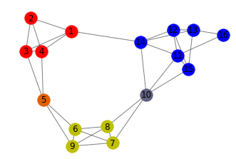
Figure 1: Applying the Parameterized Modularity Overlap Algorithm for undirected graphs with $\theta=1$, we obtained three communities are $C_{1}=\{1,2,3,4,5\}$, $C_{2}=\{5,6,7,8,9,10\}$, and $C_{3}=\{10,11,12,13,14,15,16\}$. Vertex $5$ belongs to communities $C_{1}$ and $C_{2}$. Vertex $10$ belongs to both communities $C_{2}$ and $C_{3}$.

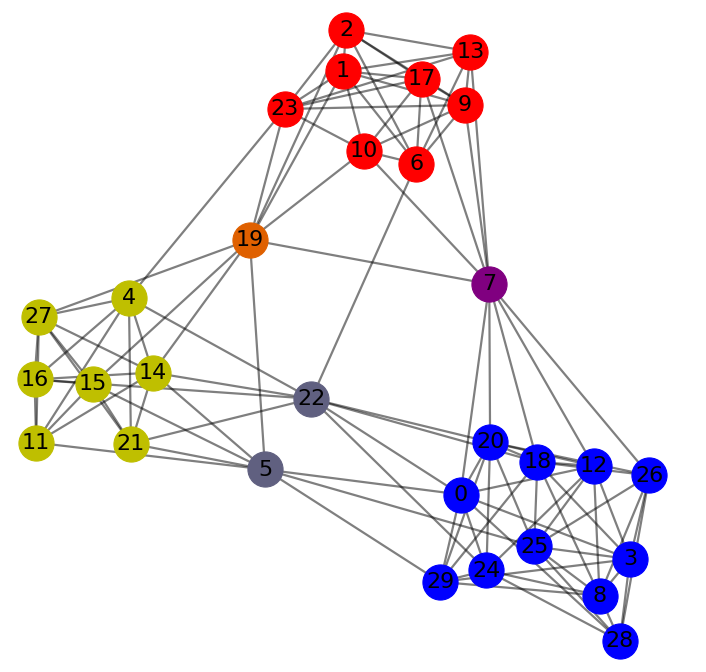
Figure 2: Applying the Cosine Overlap Algorithm with $\theta=0.6$, we obtained three communities $C1=\{4,5,11,14,15,16,21,22,27,19\}$, $C2=\{1,2,6,7,9,10,13,17,19,23\}$ and $C3=\{0,3,8,12,18,20,24,25,26,28,29,5,7,22\}$. Vertex $19$ belongs to communities $C_{1}$ and $C_{2}$. Vertex $7$ belongs to both communities $C_{2}$ and $C_{3}$, and vertices $5$, $22$ belongs to both communities $C_{1}$ and $C_{3}$.

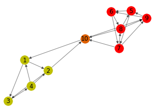
Figure 3: Applying the Parameterized Modularity Overlap Algorithm for directed graphs with $\theta=1$, we obtained two communities $C_{1}=\{1,2,3,4,10\}$ and $C_{2}=\{5,6,7,8,9,10\}$. Vertex $10$ belongs to communities $C_{1}$ and $C_{2}$.

5 Experiments

We will evaluate the effectiveness and rationality of our algorithms by conducting experiments to compare and consider the clustering results of our algorithms with other algorithms and the clustering generated by the graph generation model. Specifically: In Subsection 5.2.2, we will compare two of our algorithms for undirected graphs, namely the Parameterized Modularity Overlap Algorithm (proposed in Subsection 2.1) and the Cosine Overlap Algorithm (proposed in Subsection 3.1), with four other algorithms. In which the two algorithms we introduced in the previous section are the Parameterized Overlap Algorithm [37] and the Module Overlap Algorithm [10]. Moreover, we also compare our algorithms with two famous algorithms, the Bigclam algorithm [44] and the Copra algorithm [19].

We will compare these algorithms based on Modularity and ONMI. Additionally, we will perform experiments on real datasets and compare the algorithms based on Modularity. Subsection 5.2.3, we will apply our directed graph algorithms to randomly generated graphs and compare the results with the clustering generated by the graph generation model based on ONMI.

5.1 Evaluating metrics

Modularity for undirected graphs with overlapping communities:

Chen et al. [10] provide the generalized modularity-based belonging function for calculating modularity in undirected graphs. The following equation represents this function:

$$Q=\frac{1}{2m}\sum_{C_{j}\in C}\sum_{u,v\in C_{j}}\left(A_{uv}-\frac{d_{u}d_{v}}{2m}\right)f\left(\alpha_{uC_{j}},\alpha_{vC_{j}}\right).$$ (5.1)

where $\alpha_{uC_{j}}$ is defined as in the Equation (1.2). The belonging coefficient function $f\left(\alpha_{uC_{j}},\alpha_{vC_{j}}\right)$ can be the product or average of $\alpha_{uC_{j}},\alpha_{vC_{j}}$. If it is average, it becomes the following equation.

$$Q=\frac{1}{2m}\sum_{C_{j}\in C}\sum_{u,v\in V}\left(A_{uv}-\frac{d_{u}d_{v}}{2m}\right)\left(\alpha_{uC_{j}}+\alpha_{uC_{j}}\right)/2.$$ (5.2)

In this part of the experiment, we will use this modularity to evaluate the clustering quality.

The Overlapping Normalized Mutual Information (ONMI):

The Overlapping Normalized Mutual Information [28] is a measure used to evaluate the similarity between two clusters or data organizations. It considers both the overlap between clusters and the similarity between labels within the clusters. The formula to compute ONMI is as follows:

$$ONMI(A,B)=\dfrac{2\,MI(A,B)}{H(A)+H(B)},$$ (5.3)

where, $MI(A,B)$ represents the Mutual Information (MI) between the two clusters $A$ and $B$. $H(A)$ and $H(B)$ denote the entropy of clusters $A$ and $B$, respectively. Mutual Information (MI) measures the dependence between two random variables. It is calculated by summing the joint probabilities of pairs of values for the two variables multiplied by the logarithm of the ratio between the joint probability and the product of the individual probabilities. Entropy quantifies the uncertainty in a random variable. The entropy of a cluster is calculated by summing the probabilities of the labels within the cluster multiplied by the logarithm of that probability.

5.2 The random graph model and experiments on random graphs

5.2.1 The random graph model

Evaluating a community detection algorithm is difficult because one needs some test graphs whose community structure is already known. A classical approach is to use randomly generated graphs with labeled communities. Here we will use this approach and generate the graphs as follows.
LFR benchmark graphs: This random graph generator model creates community-structured graphs with overlapping vertices. Andrea Lancichinetti and Santo Fortunato proposed it in [25]. This model generates graphs with many of the same properties as real networks. To create the graphs, we need the following parameters:

• N: number of nodes.

• k: average degree.

• maxk: maximum degree.

• $\mu$: mixing parameter.

• $t_{1}$: minus exponent for the degree sequence.

• $t_{2}$: minus exponent for the community size distribution.

• minc: minimum for the community sizes.

• maxc: maximum for the community sizes.

• on: number of overlapping nodes.

• om: number of memberships of the overlapping nodes.

When applying, we take the parameters $t_{1}=2$, $t_{2}=1$. This random graph generation model can generate both undirected and directed graphs.

5.2.2 Experiments on random graphs for undirected graphs

In this part of the experiment, each table results from experiments on ten randomly generated graphs using the LFR benchmark graphs mode. We will conduct experiments on all six algorithms for the ten graphs generated. For each Algorithm except the Bigclam algorithm, we will perform 20 experiments corresponding to 20 different parameters and select the clustering result with the highest Modularity and ONMI among those experiments. Specifically, the parameters for each Algorithm will be as follows:

• Parameterized Modularity Overlap Algorithm: we will use the coefficient $\theta=1+0.1t$ with $t\in\{1,2,\dots,20\}$.

• Cosine Overlap Algorithm: we will use the coefficient $\theta=0.2+0.035t$ with $t\in\{1,2,\dots,20\}$.

• Parameterized Overlap Algorithm: we will use the coefficient $\theta=0.2+0.015t$ with $t\in\{1,2,\dots,20\}$.

• Module Overlap Algorithm: we will set the coefficient $B^{U}$ to 0.5 and use the coefficient $B^{L}=0.2+0.015t$ with $t\in\{1,2,\dots,20\}$.

• Copra Algorithm: We will apply the Copra algorithm 20 times to each graph and get the best result out of those 20 experiments. To increase the algorithm’s accuracy, we choose the parameter $v$ in the algorithm to be the number generated by creating the graph and the parameter $T$ to be 15.

• Bigclam Algorithm: To improve the algorithm’s accuracy, we choose the parameter $K$ (number of communities), which is the number of communities generated by random graph generation.

We will evaluate the efficiency of algorithms using two metrics: modularity (the Modularity we use is the Formula 5.2) and ONMI. In each experiment, we will first compare the maximum modularity values obtained from the clustering results obtained by each algorithm. A higher modularity value indicates a more efficient algorithm for forming well-defined communities. Next, we will compare the clustering results obtained by each algorithm with the original clustering generated by the graph generation (original clustering) based on ONMI. ONMI measures the similarity between two sets of clusters, with a value close to 1 indicating a strong resemblance between the obtained and original clustering. When the obtained clustering matches the original clustering, the ONMI value will be 1. By employing both modularity and ONMI, we can assess the algorithm’s effectiveness in forming cohesive communities and its ability to generate clustering results that closely align with the ground-truth clustering.

In the LFR benchmark graphs model, the coefficient $\mu\in[0,1]$ determines the clarity of the community structure. When $\mu$ is close to 0, the graph exhibits a clear community structure with well-defined communities. On the other hand, when $\mu$ approaches 1, the generated graph shows little to no community structure, with a high level of overlap between communities. To thoroughly explore the algorithm’s behavior, we will test it in each experiment on various values of $\mu$. Specifically, we will experiment with the following values of $\mu$: $\mu\in\{0.05,0.075,0.1,0.2,0.3,0.4\}$. By testing the algorithm on these different values of $\mu$, we can analyze its performance under various community structure scenarios, ranging from clear to overlapping communities.

Experiment 1 for undirected graphs:

We will experiment on ten randomly generated graphs using the LFR benchmark with all the parameters taken with a uniform distribution in the following corresponding intervals: $N\in[400;500]$, $k\in[6;8]$, $maxk\in[8;16]$, $on\in[60;80]$, $om\in[2;5]$, $minc\in[30;50]$, and $maxc\in[50;80]$.

We have illustrated the results obtained from this experiment as shown in Figures 4, 5. In the scenario where a graph consists of approximately 400 to 500 vertices, with an overlap of 60 to 80 vertices, our two algorithms still have been shown to yield the maximum modularity value and ONMI value in most cases. Among these algorithms, the Cosine Overlap Algorithm has the best results.

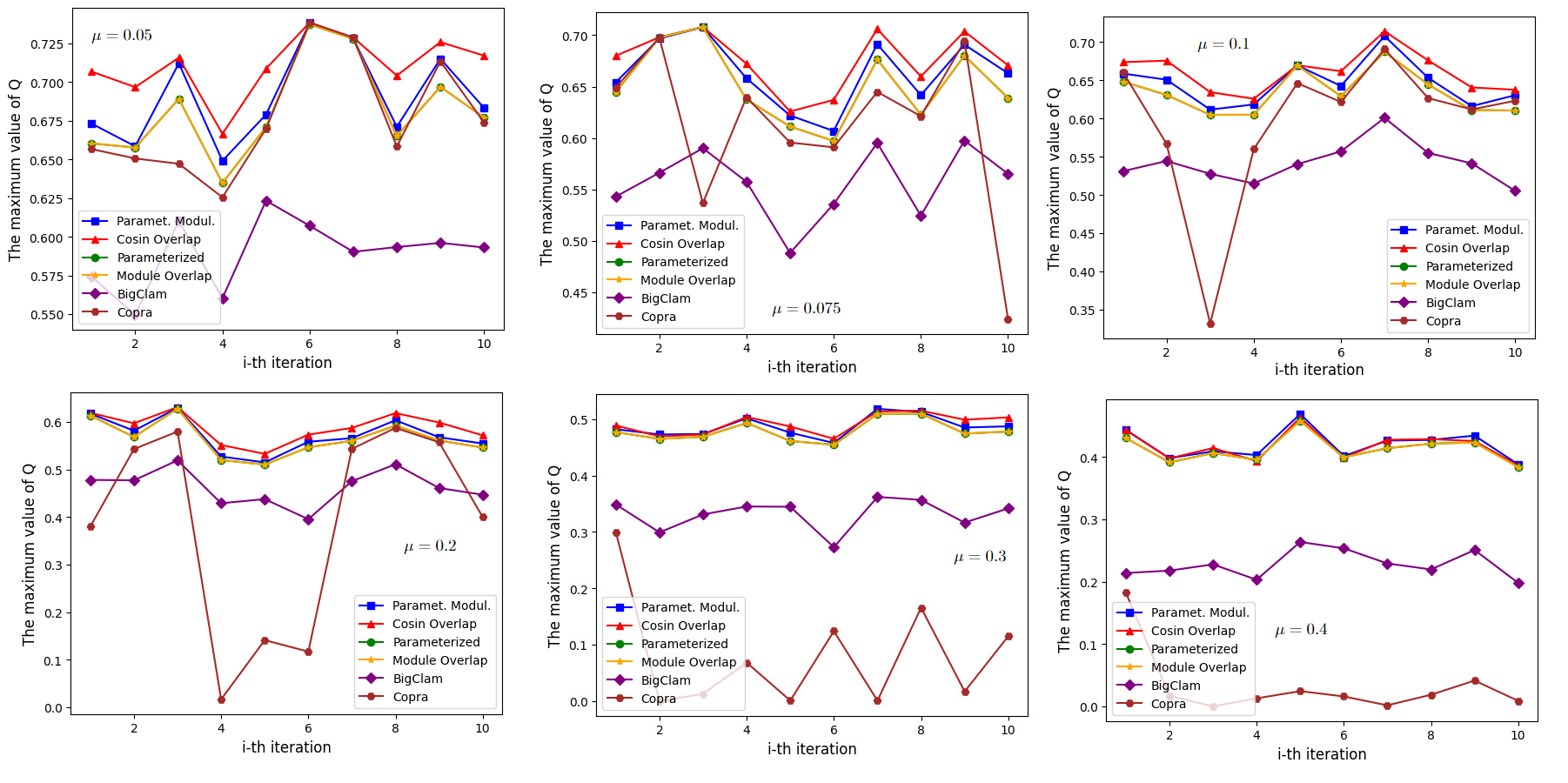
Figure 4: This chart illustrates the maximum modularity obtained in Experiment 1 for undirected graphs; we experimented on ten randomly generated graphs using the LFR benchmark with all the parameters taken with a uniform distribution in the following corresponding intervals: $N\in[400;500]$, $on\in[60;80]$, $om\in[2;5]$.

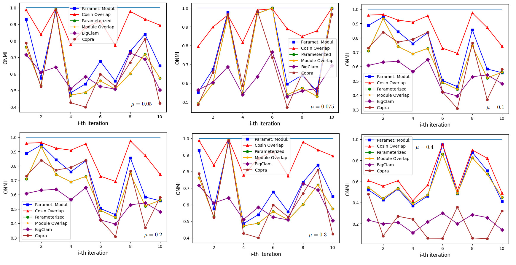
Figure 5: This chart illustrates the maximum ONMI obtained in Experiment 1 for undirected graphs; we experimented on ten randomly generated graphs using the LFR benchmark with all the parameters taken with a uniform distribution in the following corresponding intervals: $N\in[400;500]$, $on\in[60;80]$, $om\in[2;5]$.

Experiment 2 for undirected graphs:

We will experiment on ten randomly generated graphs using the LFR benchmark with all the parameters taken with a uniform distribution in the following corresponding intervals: $N\in[800;1000]$, $k\in[6;10]$, $maxk\in[10;20]$, $on\in[80;100]$, $om\in[2;5]$, $minc\in[70;100]$, and $maxc\in[100;150]$.

Despite increasing the number of peaks in the graphs to approximately 800 to 1000, we could replicate the same results from the previous two experiments. We present these results in Figures 6, 7.

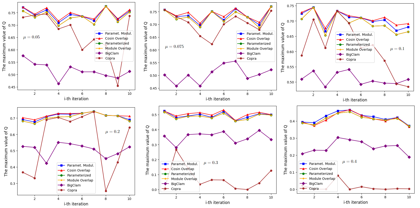
Figure 6: This chart illustratesthe maximum modularity obtained in Experiment 2 for undirected graphs; we experimented on ten randomly generated graphs using the LFR benchmark with all the parameters taken with a uniform distribution in the following corresponding intervals: $N\in[800;1000]$, $on\in[80;100]$, $om\in[2;5]$.

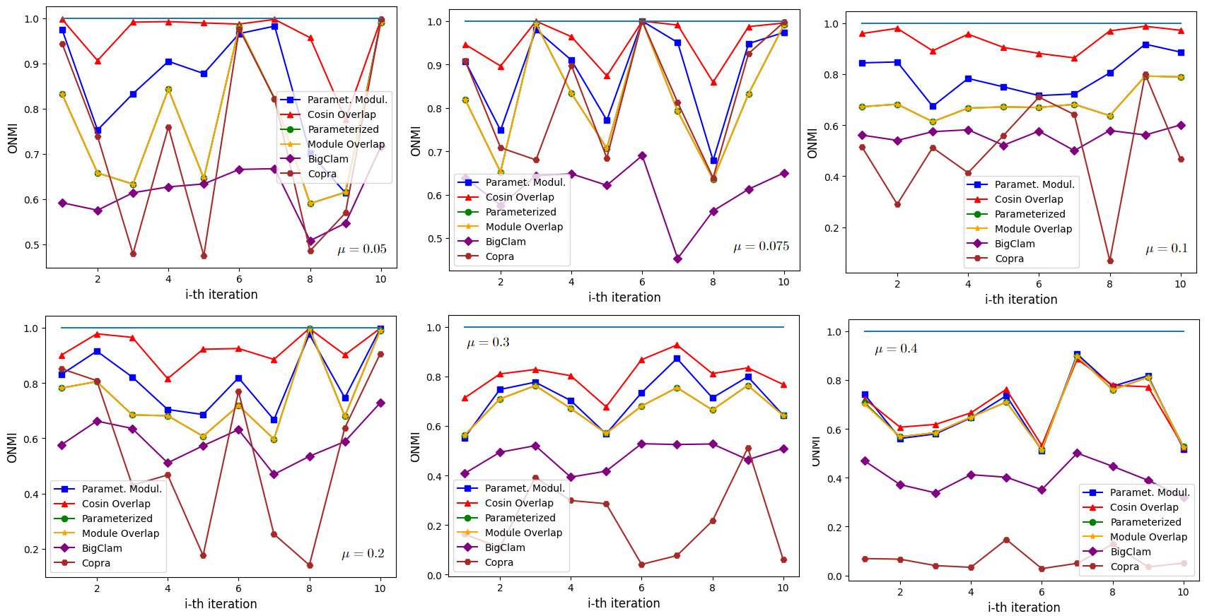
Figure 7: This chart illustratesthe maximum ONMI obtained in Experiment 2 for undirected graphs; we experimented on ten randomly generated graphsusing the LFR benchmark with all the parameters taken with a uniform distribution in the following corresponding intervals: $N\in[800;1000]$, $on\in[80;100]$, $om\in[2;5]$.

Experiment 3 for undirected graphs:

We will experiment on ten randomly generated graphs using the LFR benchmark with all the parameters taken with a uniform distribution in the following corresponding intervals: $N\in[2000;3000]$, $k\in[10;20]$, $maxk\in[20;30]$, $on\in[200;300]$, $om\in[2;5]$, $minc\in[200;300]$, and $maxc\in[300;500]$.

Despite increasing the number of peaks in the graphs to approximately 800 to 1000, we could replicate the same results from the previous two experiments. We present these results in Figures 8, 9.

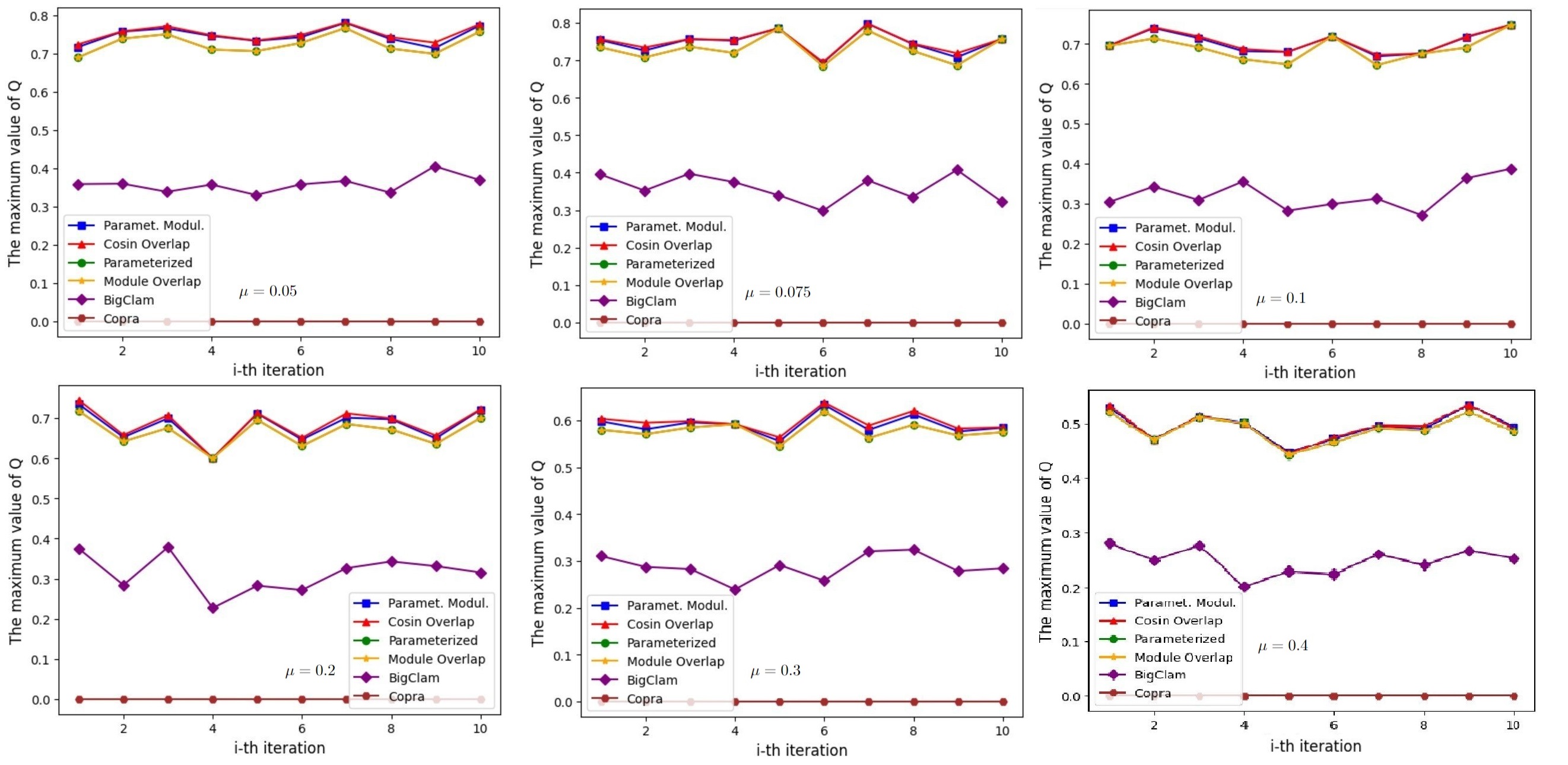
Figure 8: This chart illustratesthe maximum modularity obtained in Experiment 3 for undirected graphs; we experimented on ten randomly generated graphs using the LFR benchmark with all the parameters taken with a uniform distribution in the following corresponding intervals: $N\in[2000;3000]$, $on\in[200;300]$, $om\in[2;5]$.

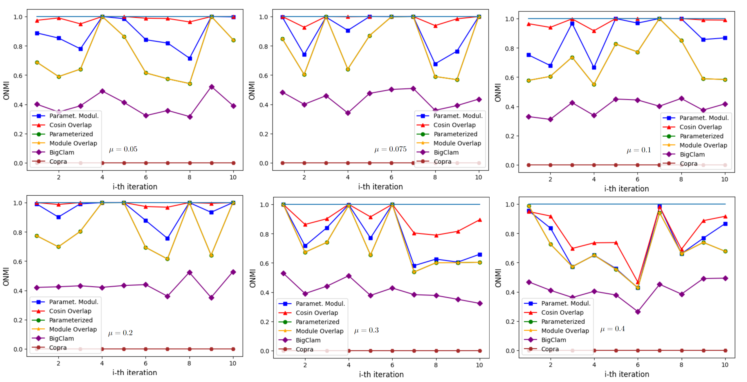
Figure 9: This chart illustratesthe maximum ONMI obtained in Experiment 3 for undirected graphs; we experimented on ten randomly generated graphs using the LFR benchmark with all the parameters taken with a uniform distribution in the following corresponding intervals: $N\in[2000;3000]$, $on\in[200;300]$, $om\in[2;5]$.

Experiment 4 for undirected graphs:

We will experiment on ten randomly generated graphs using the LFR benchmark with all the parameters taken with a uniform distribution in the following corresponding intervals: $N\in[5000;10000]$, $k\in[10;20]$, $maxk\in[20;30]$, $on\in[200;300]$, $om\in[2;5]$, $minc\in[200;300]$, and $maxc\in[300;500]$.

Despite increasing the number of peaks in the graphs to approximately 5000 to 10000, we could replicate the same results from the previous two experiments. We present these results in Figures 10, 11.

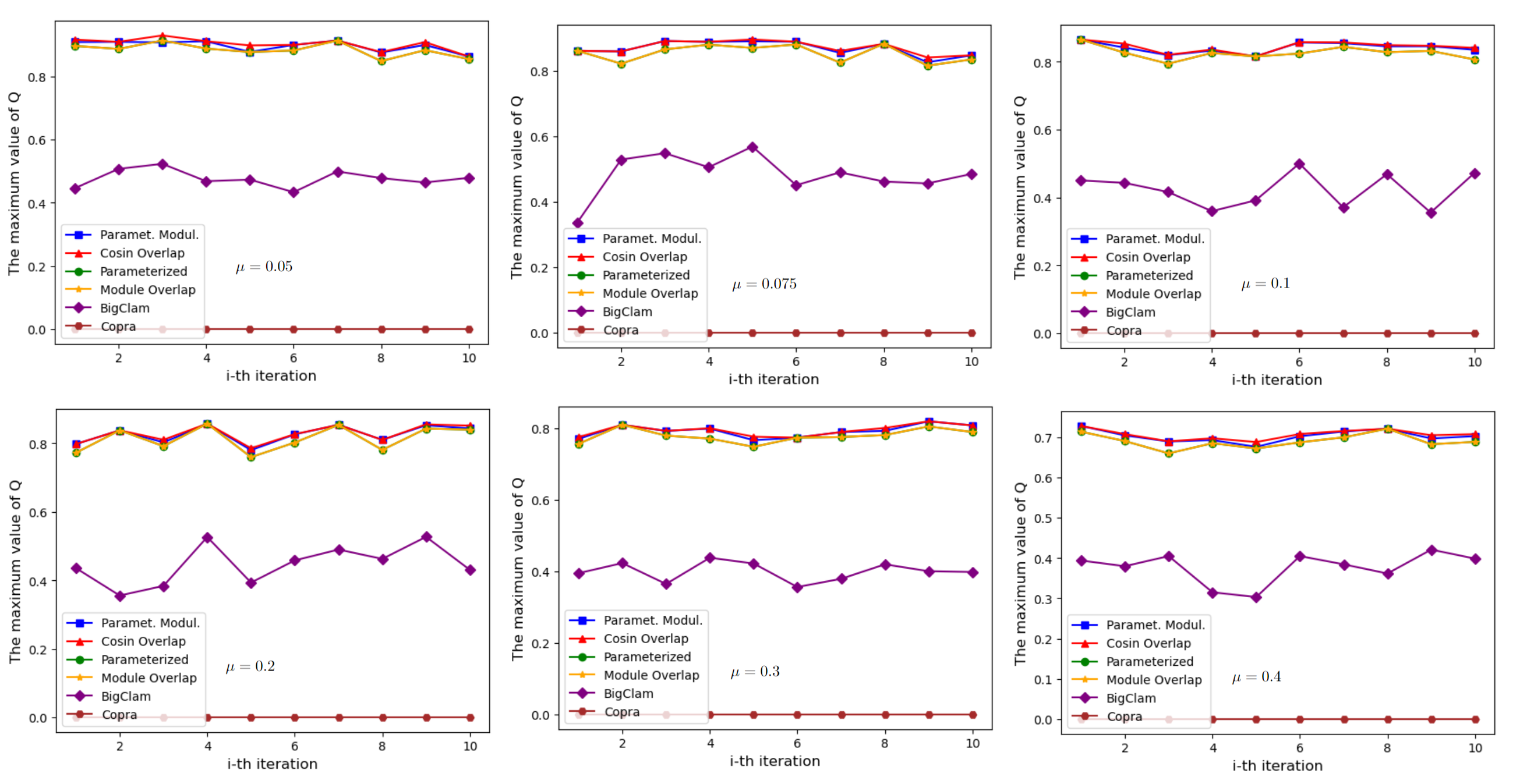
Figure 10: This chart illustratesthe maximum modularity obtained in Experiment 4 for undirected graphs; we experimented on ten randomly generated graphs using the LFR benchmark with all the parameters taken with a uniform distribution in the following corresponding intervals: $N\in[5000;10000]$, $on\in[200;300]$, $om\in[2;5]$.

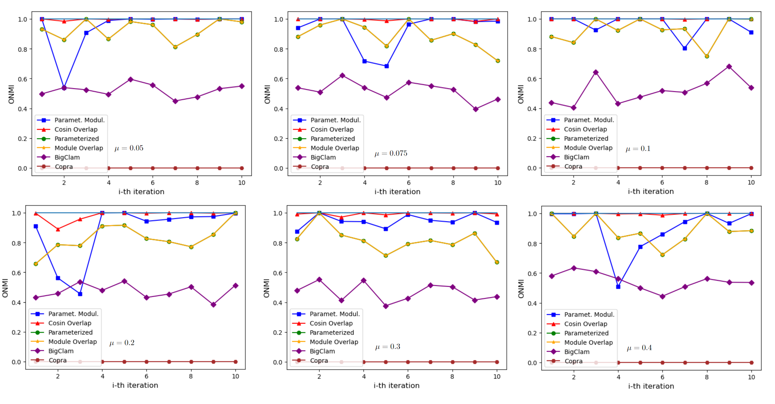
Figure 11: This chart illustratesthe maximum ONMI obtained in Experiment 4 for undirected graphs; we experimented on ten randomly generated graphs using the LFR benchmark with all the parameters taken with a uniform distribution in the following corresponding intervals: $N\in[5000;10000]$, $on\in[200;300]$, $om\in[2;5]$.

5.2.3 Experiments on random graphs for directed graphs

In the following experiments, we will utilize our three algorithms (Directed Parameterized d-Modularity Overlap Algorithm, Directed Parameterized sd-Modularity Overlap Algorithm, and Directed Cosine Overlap Algorithm) for directed graphs to cluster random generation graphs. Subsequently, we will compare the index obtained from our algorithms with the graph generation index. The parameters for each Algorithm will be as follows:

• Directed Parameterized d-Modularity Overlap Algorithm: we will use the coefficient $\theta=1+0.1t$ with $t\in\{1,2,\dots,20\}$.

• Directed Parameterized sd-Modularity Overlap Algorithm: we will use the coefficient $\theta=1+0.1t$ with $t\in\{1,2,\dots,20\}$.

• Directed Cosine Overlap Algorithm: we will use the coefficient $\theta=0.2+0.035t$ with $t\in\{1,2,\dots,20\}$.

We will compare the clustering results obtained by each algorithm with the original clustering generated by the graph generation (original clustering) based on ONMI (the ONMI we use is the Formula 5.3). ONMI measures the similarity between two sets of clusters, with a value close to 1 indicating a strong resemblance between the obtained and original clustering. When the obtained clustering matches the original clustering, the ONMI value will be 1. We will select the clustering result for each algorithm corresponding to the parameter value that obtained the highest ONMI value.

Experiment 1 for directed graphs:

We will experiment on ten randomly generated graphs using the LFR benchmark with all the parameters taken with a uniform distribution in the following corresponding intervals: $N\in[400;500]$, $k\in[6;10]$, $maxk\in[10;15]$, $on\in[20;30]$, $om\in[2;5]$, $minc\in[30;50]$, and $maxc\in[50;80]$.

This experiment will investigate the number of overlapping vertices identified by the algorithms and compare it with those generated by the graph generation method. That will enable us to evaluate the efficiency of our Algorithm. We present the results of Experiment 1 in Figure 12.

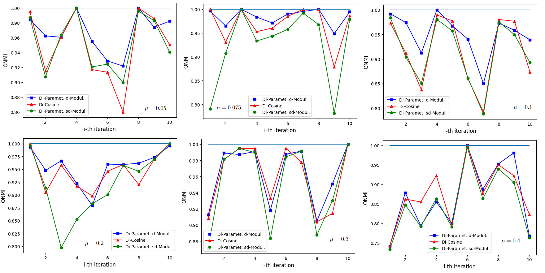
Figure 12: This chart illustrates the maximum ONMI obtained in Experiment 1 for directed graphs; we experimented on ten randomly generated graphs using the LFR benchmark with all the parameters taken with a uniform distribution in the following corresponding intervals: $N\in[400;500]$, $on\in[20;30]$, $om\in[2;5]$.

Experiment 2 for directed graphs:

We will experiment on ten randomly generated graphs using the LFR benchmark with all the parameters taken with a uniform distribution in the following corresponding intervals: $N\in[800;1000]$, $k\in[8;15]$, $maxk\in[15;20]$, $on\in[40;50]$, $om\in[2;5]$, $minc\in[80;100]$, and $maxc\in[100;150]$.

This experiment will investigate the number of overlapping vertices identified by the algorithms and compare it with those generated by the graph generation method. That will enable us to evaluate the efficiency of our Algorithm. We present the results of Experiment 2 in Figure 13.

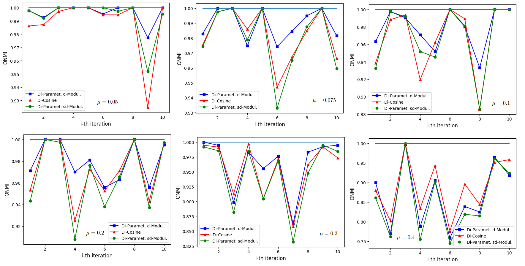
Figure 13: This chart illustrates the maximum ONMI obtained in Experiment 2 for directed graphs; we experimented on ten randomly generated graphs using the LFR benchmark with all the parameters taken with a uniform distribution in the following corresponding intervals: $N\in[800;1000]$, $on\in[40;50]$, $om\in[2;5]$.

Experiment 3 for directed graphs:

We will experiment on ten randomly generated graphs using the LFR benchmark with all the parameters taken with a uniform distribution in the following corresponding intervals: $N\in[2000;3000]$, $k\in[10;20]$, $maxk\in[20;30]$, $on\in[100;150]$, $om\in[2;5]$, $minc\in[100;200]$, and $maxc\in[300;500]$.

This experiment will investigate the number of overlapping vertices identified by the algorithms and compare it with those generated by the graph generation method. That will enable us to evaluate the efficiency of our Algorithm. We present the results of Experiment 3 in Figure 14.

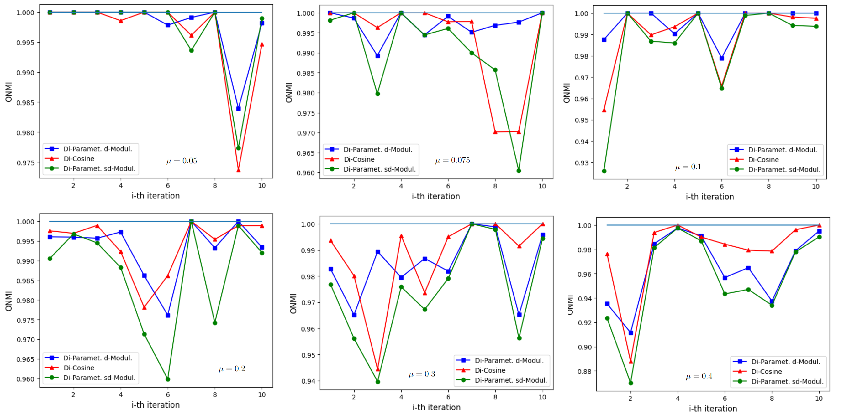
Figure 14: This chart illustrates the maximum ONMI obtained in Experiment 4 for directed graphs; we experimented on ten randomly generated graphs using the LFR benchmark with all the parameters taken with a uniform distribution in the following corresponding intervals: $N\in[2000;3000]$, $on\in[100;150]$, $om\in[2;5]$.

Experiment 4 for directed graphs:

We will experiment on ten randomly generated graphs using the LFR benchmark with all the parameters taken with a uniform distribution in the following corresponding intervals: $N\in[5000;10000]$, $k\in[10;30]$, $maxk\in[30;50]$, $on\in[100;150]$, $om\in[2;5]$, $minc\in[100;200]$, and $maxc\in[300;500]$.

This experiment will investigate the number of overlapping vertices identified by the algorithms and compare it with those generated by the graph generation method. That will enable us to evaluate the efficiency of our Algorithm. We present the results of Experiment 4 in Figure 15.

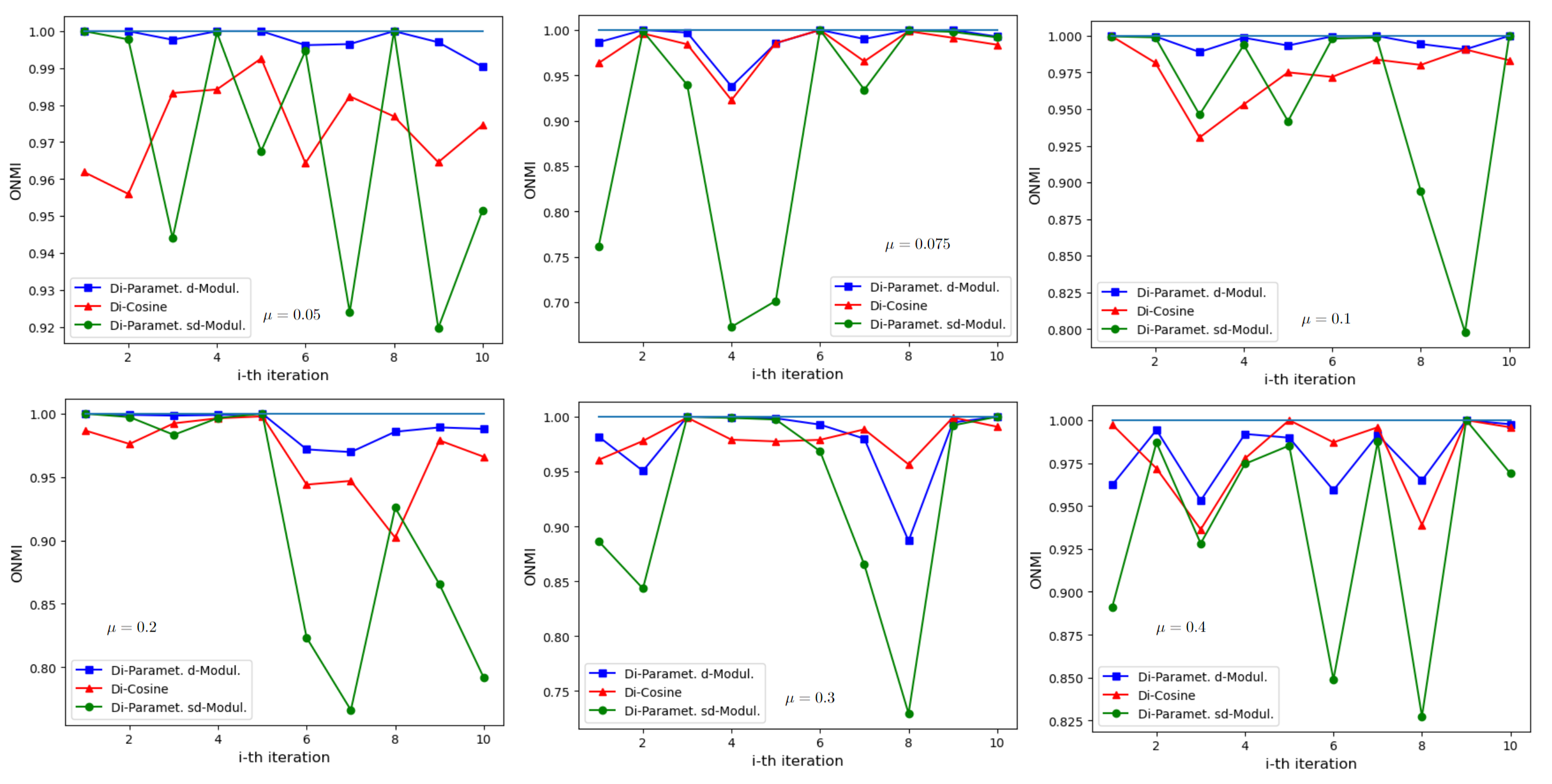
Figure 15: This chart illustrates the maximum ONMI obtained in Experiment 4 for directed graphs; we experimented on ten randomly generated graphs using the LFR benchmark with all the parameters taken with a uniform distribution in the following corresponding intervals: $N\in[5000;10000]$, $on\in[100;150]$, $om\in[2;5]$.

5.3 Real data and experiments on real data

5.3.1 Real data

In this paper, we will perform experiments on the following famous real data.
Zachary’s karate club: Wayne W. Zachary studied a social network of a karate club over three years from 1970 to 1972, as a paper in [46]. The network represents 34 members, recording the connections between pairs of members who had interactions beyond the club’s premises. After being utilized by Michelle Girvan and Mark Newman in 2002 [16], the network became a widely-used example of community structure in networks.
Dolphin’s associations: The dataset used in this study was obtained from [26]. It describes the connections between 62 dolphins living in Doubtful Sound, New Zealand, where the links between pairs of dolphins represent statistically significant frequent associations. This network can be naturally divided into two distinct groups.
Metabolic network: According to [20], a metabolic network represents the comprehensive collection of metabolic and physical processes that dictate a cell’s physiological and biochemical characteristics. Therefore, these networks consist of metabolic reactions, pathways, and the regulatory interactions that direct these reactions.

In addition, we will also perform experiments on the following real data: Jazz network in [47]. Email network [17]. College football in [16]. Hamster households, hamster friendships, DNC co-recipient, and Asoiaf in [24].

5.3.2 Experiments on real data

We will conduct experiments on all six algorithms for each real network. We will perform 20 experiments with 20 different parameters for each Algorithm and select the clustering result with the highest Modularity among those experiments. Specifically, the parameters for each Algorithm will be set as follows:

• Parameterized Modularity Overlap Algorithm: we will use the coefficient $\theta=1+0.1t$ with $t\in\{1,2,\dots,20\}$.

• Cosine Overlap Algorithm: we will use the coefficient $\theta=0.2+0.035t$ with $t\in\{1,2,\dots,20\}$.

• Parameterized Overlap Algorithm: we will use the coefficient $\theta=0.2+0.015t$ with $t\in\{1,2,\dots,20\}$.

• Module Overlap Algorithm: we will set the coefficient $B^{U}$ to 0.5 and use the coefficient $B^{L}=0.2+0.015t$ with $t\in\{1,2,\dots,20\}$.

• Copra Algorithm: We will execute the algorithm with each graph nine times, varying the parameter $V$ from 2 to 10 and keeping the parameter $T$ fixed at 15. After running these nine experiments, we will select the best result obtained among these runs. We will do this 20 times and choose the best result.

• Bigclam Algorithm: In each experiment, we will conduct form 5 to 20 runs of the algorithm, each with a different value for the parameter $K$ (number of communities). After running these 20 experiments, we will select the best result obtained from these runs. The values of the $K$ parameter will be chosen based on the size of the networks. For instance, in the case of the Karate network and the Dolphin network, we will consider values of $K$ ranging from 2 to 6.

Graph, $G=(|V|,|E|)$	Paramet. Modul. overlap	Cosine Overlap	Paramet. Overlap	Module Overlap	BigClam	Copra
Dolphin’s associations [26], $G=(62,159)$	0.5318953	0.5309415	0.5282947	0.5282947	0.4138026	0.4276747
Zachary’s karate club [46], $G=(34,78)$	0.4300419	0.4197896	0.4267998	0.4267998	0.2741145	0.3920940
Metabolic network [20], $G=(453,2025)$	0.4542220	0.4385402	0.4501564	0.4447795	0.2680016	0.0402168
College football [16], $G=(115,613)$	0.6103202	0.6077106	0.6056203	0.6044072	0.5730757	0.5913225
Jazz network [18], $G=(198,2742)$	0.4551599	0.4498614	0.4473198	0.4463121	0.3641616	0.2528598
Email network [17], $G=(1133,5451)$	0.5900769	0.5905986	0.5900962	0.5786008	0.3961421	0.4997626
Hamster households [24], $G=(921,4032)$	0.3804496	0.3658147	0.3782052	0.3774382	0.1210200	0.0293135
Hamsters friendships [24], $G=(1858,12534)$	0.4692017	0.4512992	0.4537756	0.4547541	0.3424725	0.2063043
DNC co-recipient [24], $G=(906,10429)$	0.4434152	0.4420661	0.4419830	0.4419830	0.2838478	0.1822132
Asoiaf [24], $G=(796,2823)$	0.6062354	0.6097880	0.609218	0.609218	0.4247218	0.5274229

Table 1: In this table, we present the values of modularity (using the formula 5.1) corresponding to the clustering results of the algorithms.

5.4 Conclusion of the experiments

The above results show that our two algorithms are efficient in almost all experiments.

• The Parameterized Modularity Overlap Algorithm consistently outperforms the Parameterized Overlap Algorithm, the Module Overlap Algorithm, Bigclam Algorithm, and Copra Algorithm in most experiments. Additionally, this algorithm offers the advantage of having low computational complexity.

• We built The Cosine Overlap Algorithm by observing the network’s relationship between random walks and community structure. Although the computational complexity will be greater than the Parameterized Modularity Overlap Algorithm, all experiments on the Cosine algorithm randomization graph are for the best results. Furthermore, the Algorithm makes a lot of sense in theory and is an interesting algorithm that deserves attention.

• Our algorithms for undirected graphs exhibit better performance compared to the other four algorithms, particularly when each overlapping vertex belongs to more than two communities. Additionally, in the case of graphs with a clear community structure, Cosine Overlap Algorithm consistently outperforms all other algorithms, producing superior results.

• Our directed graph algorithms demonstrate remarkable efficiency compared to the indices generated based on the graph generation method. Especially the Directed Cosine Overlap Algorithm, in most cases, gets the best results.

6 Conclusion and further work

In this paper, we have proposed two algorithms for overlapping community detection for undirected and directed graphs; our algorithms go through 2 steps. In step 1, we separate community detection using the algorithms we know, such as the Hitting times Walktrap algorithm, NL-PCA algorithm[11], Walktrap algorithm [38] or Louvain algorithm [42]. In step 2, we look for overlapping communities. Specifically, we have proposed the following two algorithms.

• The Parameterized Modularity Overlap Algorithm uses the idea that vertex $u$ belongs to the community $C_{j}$ if the sum of the probabilities from vertex $u$ to the community $C_{j}$ and the probabilities from community $C_{j}$ to vertex $u$ is large enough.

• In the Cosine Overlap Algorithm, we first coordinate the vertices of the graph, then find the centers of the clusters and use the idea that the vertex $u$ belongs to the cluster $C_{j}$ if the angle between the vector corresponds to the vertex $u$ and the center of the cluster $C_{j}$ is small.

We also performed experiments on random generative graphs and real data to compare with Module Overlap algorithm, Parameterized Overlap algorithm, Bigclam algorithm, and Copra algorithm; the result is that our algorithms give better results when using the modularity and ONMI measures.

In the future, we will continue to study the problem of finding overlapping communities based on two vertices belonging to a community through other criteria, such as using cut, distance, and cosine.

References

- [1] L. A. N. Amaral, A. Scala, M. Barth’el’emy, and H. E. Stanley, Classes of small-world networks. Proc. Natl. Acad. Sci. USA 97, 11149–11152 (2000).
- [2] A. Arenas, J. Duch, A. Fernandez, and S. Gomez. Size reduction of complex networks preserving Modularity. New Journal of Physics, 9:176, 2007.
- [3] A. L. Barabasi and R. Albert, Emergence of scaling in random networks. Science 286, 509–512, 1999.
- [4] S. Boccaletti, V. Latora, Y. Moreno, M. Chavez, and D.- U. Hwang, Complex networks: Structure and dynamics, Physics Reports, Volume 424, Issues 4–5, 175-308, 2006.
- [5] S. Brin, L. Page, The anatomy of a large-scale hypertextual web search engine, Comput. Netw. ISDN Syst. 30 (1-7), 107–117, 1998.
- [6] D. S. Callaway, M. E. J. Newman, S. H. Strogatz, and D. J. Watts, Network robustness and fragility: Percolation on random graphs. Phys. Rev. Lett. 85, 5468–5471 2000.
- [7] A. Clauset, C. Moore, and M. E. J. Newman, Hierarchical structure and the prediction of missing links in networks. Nature 453, 98–101, 2008.
- [8] R. Cohen, K. Erez, D. ben-Avraham, and S. Havlin, Re- silence of the Internet to random breakdowns. Phys. Rev. Lett. 85, 4626–4628, 2000.
- [9] M. B. Cohen, J. Kelner, J. Peebles, R. Peng, A. Sidford, A. Vladu, Faster Algorithms for Computing the Stationary Distribution, Simulating Random Walks, and More, Annual IEEE Symposium on Foundations of Computer Science, 2016, Page(s):583 - 592.
- [10] D. Chen, M. Shang, Z. Lu, and Y. Fu, Detecting Overlapping Communities of Weighted Networks via a Local Algorithm, Physica A: Statistical Mechanics and its Applications, vol. 389, no. 19, pp. 4177–4187, 2010.
- [11] D. T. Dat, D. D. Hieu and P. T. H. Duong, Community detection in directed graphs using stationary distribution and hitting times methods, Social Network Analysis and Mining volume 13, Article number: 80, 2023.
- [12] N. Dugué and A. Perez, Directed Louvain: maximizing modularity in directed networks. [Research Report] Université d’Orléans, 2015.
- [13] B. S. Everitt, S. Landau, and M. Leese. Cluster Analysis. Hodder Arnold, London, 4th edition, 2001.
- [14] G. W. Flake, S. Lawrence, C. L. Giles, and F. M. Coetzee. Self-organization and identification of web communities. Computer, 35(3):66-71, 2002.
- [15] S. Fortunato, ”Community detection in graphs,” Physics Reports, vol. 486, pp. 75–174, 2010.
- [16] M. Girvan, M.E.J Newman, Community structure in social and biological networks, Proc. Natl. Acad. Sci. USA 99 (2002) 7821–7826
- [17] R. Guimerà, L. Danon, A. Díaz-Guilera, F. Giralt, and A. Arenas. Self-similar community structure in a network of human interactions. Phys. Rev. E, 68(6):065103, 2003.
- [18] Gleiser, P. M. and Danon, L. Community structure in jazz. Adv. Complex. Syst. 6, 565–573, 2003.
- [19] S. Gregor, Finding overlapping communities in networks by label propagation, New Journal of Physics, Volume 12, October 2010.
- [20] Jeong, H., Tombor, B., Albert, R., Oltvai, Z. N. and Barabási, A.-L. The large-scale organization of metabolic networks. Nature 407, 651–654, 2000.
- [21] S. Harenberg,G. Bello, L. Gjeltema, S. Ranshous, J. Harlalka, R. Seay, K. Padmanabhan, N. Samatova. Community detection in large-scale networks: a survey and empirical evaluation. WIREs Comput Stat 6(6):426–439, 2014.
- [22] J. Kleinberg and S. Lawrence. The structure of the web. Science,
- [23] M. Jebabli, H. Cherifi,C. Cherifi, A. Hamouda. Community detection algorithm evaluation with ground-truth data. Physica A Stat Mech Appl 492:651–706.2018.
- [24] J. Kunegis. KONECT – The Koblenz Network Collection. In Proc. Int. Conf. on World Wide Web Companion, pages 1343–1350, 2013.
- [25] A. Lancichinetti and S. Fortunato, Benchmarks for testing community detection algorithms on directed and weighted graphs with overlapping communities, Phys. Rev. E 80, 016118 – Published 31 July 2009.
- [26] D. Lusseau, K. Schneider, O.J. Boisseau, P. Haase, E. Slooten, S.M. Dawson, The bottlenose dolphin community of doubtful sound features a large proportion of long-lasting associations, Behav. Ecol. Sociobiol. 54 (2003) 396–405.
- [27] E. A. Leicht and M. E. J. Newman. Community structure in directed networks. Physical Review Letter, 100:118703, 2008.
- [28] AF. McDaid, D. Greene, N. Hurley, Normalized mutual information to evaluate overlapping community finding algorithms. https://doi.org/1110.2515 (2011), Accessed 06 Jan 2020.
- [29] M.E.J. Newman and M. Girvan, Finding and evaluating community structure in networks, Phys. Rev. E 69, 026–11, 2004.
- [30] M. E. J. Newman, The structure and function of complex networks. SIAM Review 45, 167–256, 2003.
- [31] M. E. J. Newman, Assortative mixing in networks. Phys. Rev. Lett. 89, 208701, 2002.
- [32] V. Nicosia, G. Mangioni, V. Carchiolo, M. Malgeri, Extending the definition of Modularity to directed graphs with overlapping communities, J. Stat. Mech. P03024. 2009.
- [33] R. Pastor-Satorras, A. V´azquez, and A. Vespignani, Dynamical and correlation properties of the Internet. Phys. Rev. Lett. 87, 258701 (2001).
- [34] L. Page, S. Brin, R. Motwani, T. Winograd, The PageRank citation ranking: Bringing order to the web, in: WWW ’98: Proceedings of the 7th International World Wide Web Conference, 1998, pp. 161–172.
- [35] L. Peel, DB. Larremore, A. Clauset The ground truth about metadata and community detection in networks. Sci Adv 3(5)(2017):e1602548.
- [36] TP. Peixoto. Revealing consensus and dissensus between network partitions. https://doi.org/2005.13977, 2020.
- [37] A. Ponomarenko, L. Pitsoulis, M. Shamshetdinov. Overlapping community detection in networks based on link partitioning and partitioning around medoids. PLoS One. 2021 Aug 25;16(8):e0255717.
- [38] P. Pons and M. Latapy. Computing communities in large networks using random walks, Journal of Graph Algorithms and Applications, volume 10, no. 2, 2006, Pages 191–218, 2006.
- [39] E. Ravasz and A.-L. Barab’asi, Hierarchical organization in complex networks. Phys. Rev. E 67, 026112 (2003).
- [40] E. Ravasz, A. L. Somera, D. A. Mongru, Z. N. Oltvai, and A.-L. Barabási. Hierarchical Organization of Modularity in Metabolic Networks. Science, 297(5586):1551.
- [41] S. Sarkar and A. Dong, Community detection in graphs using singular value decomposition, Phys. Rev. E 83, 046114 – Published 21 April 2011.
- [42] BD. Vincent, G. Jean-Loup, L. Renaud and L. Etienne. Fast unfolding of communities in large networks. Journal of Statistical Mechanics: Theory and Experiment. 2008 (10): P10008.
- [43] L. Yanhua and Z. L. Zhang, Digraph Laplacian and the Degree of Asymmetry, Internet Mathematics Vol. 8, No. 4: 381–401, 2012.
- [44] J. Yang, J. Leskovec, Overlapping Community Detection at Scale: A Nonnegative Matrix Factorization Approach, Proceedings of the sixth ACM international conference on Web search and data mining. February 2013. Pages 587-596. https://doi.org/10.1145/2433396.2433471.
- [45] D. J. Watts and S. H. Strogatz, Collective dynamics of ’small-world’ networks. Nature 393, 440–442, 1998.
- [46] Zachary, W. An information flow model for conflict and fission in small groups. J. Anthropol. Res. 33, 452–473, 1977.
- [47] The Red Hot Jazz Archive, available at http://www.redhotjazz.co