The XMM Cluster Survey: Automating the estimation of hydrostatic mass for large samples of galaxy clusters I - Methodology, Validation, & Application to the SDSSRM-XCS sample

Abstract

We describe features of the X-ray: Generate and Analyse (Xga) open-source software package that have been developed to facilitate automated hydrostatic mass ($M_{\rm hydro}$) measurements from XMM X-ray observations of clusters of galaxies. This includes describing how Xga measures global, and radial, X-ray properties of galaxy clusters. We then demonstrate the reliability of Xga by comparing simple X-ray properties, namely the X-ray temperature and gas mass, with published values presented by the XMM Cluster Survey (XCS), the Ultimate XMM eXtragaLactic survey project (XXL), and the Local Cluster Substructure Survey (LoCuSS). Xga measured values for temperature are, on average, within 1% of the values reported in the literature for each sample. Xga gas masses for XXL clusters are shown to be ${\sim}$10% lower than previous measurements (though the difference is only significant at the $\sim$1.8$\sigma$ level), LoCuSS $R_{2500}$ and $R_{500}$ gas mass re-measurements are 3% and 7% lower respectively (representing 1.5$\sigma$ and 3.5$\sigma$ differences). Like-for-like comparisons of hydrostatic mass are made to LoCuSS results, which show that our measurements are $10{\pm}3\%$ ($19{\pm}7\%$) higher for $R_{2500}$ ($R_{500}$). The comparison between $R_{500}$ masses shows significant scatter. Finally, we present new $M_{\rm hydro}$ measurements for 104 clusters from the SDSS DR8 redMaPPer XCS sample (SDSSRM-XCS). Our SDSSRM-XCS hydrostatic mass measurements are in good agreement with multiple literature estimates, and represent one of the largest samples of consistently measured hydrostatic masses. We have demonstrated that Xga is a powerful tool for X-ray analysis of clusters; it will render complex-to-measure X-ray properties accessible to non-specialists.

1 Introduction

Galaxy clusters are the most massive virialized structures in the Universe. They formed through the collapse of the primordial density field, and as such are a useful way to investigate the evolution of the Universe through the measurement of cosmological parameters. The mass of a galaxy cluster is split into three main components Gonzalez et al. (2007); the dark matter halo (87%), the intra-cluster medium (7%), and the component galaxies (3%); where the intra-cluster medium (ICM) is a high-temperature, low-density plasma largely made up of ionised hydrogen. Just as the formation of clusters makes them useful for investigating cosmology, the nature of the ICM makes them ideal astrophysical laboratories.

Cosmological parameters can be derived using galaxy clusters via a variety of methods. For example, cosmological parameters have been constrained using samples of X-ray selected clusters by measuring the mass function of clusters (e.g. Vikhlinin et al., 2009; Schellenberger & Reiprich, 2017b). Therefore, one of the key properties that must be measured is the cluster mass (see Pratt et al., 2019, for a recent review). The Dark Energy Survey (DES) used galaxy clusters detected in the first year of DES observations (DESY1) to constrain cosmological parameters (Abbott et al., 2020) using a weak-lensing mass calibration (McClintock et al., 2019) and the number density of clusters. The weak lensing mass calibration for the DESY1 analysis took the form of a mass-observable relation (MOR), where the observable was the cluster richness. The richness here, symbolised by $\lambda$, is a probabilistic measure of the number of galaxies in the cluster, estimated from the red-sequence Matched-filter Probabilistic Percolation cluster finder (or redMaPPer, Rykoff et al., 2016). However, a drawback of the DESY1 analysis is the use of stacked weak lensing masses. Due to the use of a stacked analysis, information on the intrinsic scatter is lost. To enable the next generation of cluster cosmology, large scale optical/near-infrared galaxy cluster surveys will need the scatter, and normalisation, of mass-richness relations to be well calibrated. This includes the cosmology analysis that will be performed using clusters detected from the upcoming Vera Rubin Observatory’s Legacy Survey of Space and Time (LSST; e.g. see Figure G2 in The LSST Dark Energy Science Collaboration et al., 2018).

One potential method to infer the scatter of these MORs, is through the hydrostatic equilibrium mass ($M_{\rm{hydro}}$) method, using X-ray data to infer the total mass of the cluster from the temperature and gas density profiles. Of particular use to derive X-ray $M_{\rm{hydro}}$ values is the XMM-Newton telescope (hereafter XMM), whose field of view (FoV), high effective area, and large public archive of observations makes it the ideal for these measurements. Previous $M_{\rm{hydro}}$ measurements using XMM include, but are not limited to, Ettori et al. (2010); Sanderson et al. (2013); Donahue et al. (2014); Bartalucci et al. (2018); Ettori et al. (2019); Lovisari et al. (2020); Poon et al. (2023). The largest of these studies, Lovisari et al. (2020), yielded 120 $M_{\rm{hydro}}$ values. For completeness, we note that hydrostatic masses have also been measured using other (than XMM) X-ray instruments, e.g. Markevitch et al. (1998); Sarazin et al. (1998); Tamura et al. (2000); Vikhlinin et al. (2006); Sun et al. (2009); Donahue et al. (2014); Giles et al. (2017); Schellenberger & Reiprich (2017a); Logan et al. (2022); Sanders et al. (2022). The largest of these studies, Schellenberger & Reiprich (2017a), yielded 64 $M_{\rm{hydro}}$ values. Furthermore, recent efforts have been made to develop methods of estimating X-ray based masses from clusters detected in the eROSITA All Sky Survey (Scheck et al., 2023).

Gas density profiles are an important part of measuring the hydrostatic mass, but they provide a great deal of information in their own right; they are also easier to measure than hydrostatic masses. They have been measured using various X-ray telescopes, including XMM and Chandra (Croston et al., 2008; Cavagnolo et al., 2009; Bartalucci et al., 2017). The largest of these studies (Cavagnolo et al., 2009), measured profiles for 239 galaxy clusters. Other X-ray observatories have also been used, including Suzaku (Nugent et al., 2020), and ROSAT (Eckert et al., 2011; Eckert et al., 2012).

The outline of the paper is as follows. Section 2 introduces the features of the X-ray: Generate and Analyse (Xga) software package that have been developed to facilitate automated hydrostatic masses ($M_{\rm hydro}$). In Section 3, we demonstrate the reliability of the Xga measurements by comparing with published values presented by the XMM Cluster Survey (Romer et al., 2001, XCS hereafter), the Local Cluster Substructure Survey (hereafter LoCuSS), and the Ultimate XMM eXtragaLactic (hereafter XXL) survey project (Pierre et al., 2016). In Section 4, we present new $M_{\rm hydro}$ measurements of clusters in SDSS DR8 redMaPPer XCS sample. Finally, in Section 5, we present our conclusions and a discussion of the next steps of this work.

The analysis code, samples, and outputs are available in a GitHub repository. In Section 3, we adopt the cosmology parameters used in each of the original analyses to which we compare, i.e. $\Omega_{\rm{M}}$=0.3, $\Omega_{\Lambda}$=0.7, and $H_{0}$=70 km s^-1 Mpc^-1 for the XCS and LoCuSS samples (Sections 3.1.1 and 3.1.3 respectively), and $\Omega_{\rm{M}}$=0.282, $\Omega_{\Lambda}$=0.719, and $H_{0}$=69.7 km s^-1 Mpc^-1 for the XXL sample (Section 3.1.2) (i.e. the WMAP9 values in Hinshaw et al., 2013). In Section 4, we again use $\Omega_{\rm{M}}$=0.3, $\Omega_{\Lambda}$=0.7, and $\rm{H}_{0}$=70 km s^-1 Mpc^-1.

2 Methodology

The overarching aim of this work is to provide an independent mass calibration for optically selected cluster samples for the purpose of cosmological parameter estimation. The masses are estimated using X-ray observations from XMM under the assumptions of spherical symmetry and hydrostatic equilibrium (see e.g., Fabricant et al., 1980, for a derivation), following the equation

$$M_{\rm hydro}(<r)=-\dfrac{k_{B}r^{2}}{\rho_{g}(r)\mu m_{u}G}\bigg{[}\rho_{g}(r)\dfrac{dT(r)}{dr}+T(r)\dfrac{d\rho_{g}(r)}{dr}\bigg{]},$$ (1)

where $r$ is the radius within which the mass is being measured, $\rho_{g}(r)$ is the intracluster gas density profile, $T(r)$ is the gas temperature profile, $\mu=0.61$ is the mean molecular weight, $m_{u}$ is the atomic mass unit, $G$ is the gravitational constant, and $k_{B}$ is the Boltzmann constant. The quantities that need to be estimated from the XMM data are $T(r)$ and $\rho_{g}(r)$. It is important to note that these are the 3 dimensional quantities, rather than the projected (i.e. what is observed) values.

Many steps are needed to go from a raw XMM observation to an estimate of $M_{\rm hydro}$. Therefore, a secondary goal of this work is to streamline those steps into a single, self-contained workflow. Doing so ensures the consistency of the data products and allows for computational speed-ups (e.g. by making use of multi-threading on multi-core machines). The measurement tools for $M_{\rm hydro}$ that we use herein are part of the X-ray: Generate and Analyse (Xga) software suite. Xga is a generalised X-ray analysis tool, capable of investigating any X-ray source that has been observed by XMM. It was introduced in Turner et al. (2022a) and is being used in a growing number of scientific applications (e.g. Pillay et al., 2021; Turner et al., 2022b; Burke et al., 2022). It is also listed on the Astrophysics Source Code Library (ASCL; Turner et al., 2023). This work makes use of Xga v0.4.2 for all analyses, and to aid readability, the technical details about which parts of Xga are used for the different analyses in this work are described in Appendix D.

In this section, we describe each step involved in Xga $M_{\rm hydro}$ measurements. Section 2.1 explains the data inputs required to initiate Xga. Image generation and masking of contaminating sources are described in Sections 2.2 and 2.3 respectively. Manual checks of the data are outlined in Section 2.4. Section 2.5 details the generation and fitting of X-ray spectra. Correcting for the XMM point-spread function (PSF) is detailed in Section 2.6. The generation of emissivity profiles, density profiles, temperature profiles and mass profiles are outlined in Sections 2.7, 2.8, 2.10 and 2.11 respectively. To illustrate the steps, we use two example clusters: SDSSXCS-55 and SDSSXCS-6955 ($z=0.119$ and $z=0.223$ respectively). Both clusters were part of the Giles et al. (2022) study (see Section 3.1.1), but have significantly different signal to noise ratios and off axis locations in their respective XMM observations. Their properties are summarised in Table 1.

Table 1: Properties of the two galaxy clusters selected as demonstration cases for Xga. These were selected from the SDSSRM-XCS sample presented by Giles et al. (2022). The coordinates are for the XCS Xapa defined value for the UDC${}^{\ref{foot:udc}}$. This, and the $R_{2500}$ and $R_{500}$ values, in units of kpc, were taken from Giles et al. (2022). The redshift and richness values were taken from Rykoff et al. (2014) (where the numeric value in the name is the identifier in the Rykoff et al. (2014) RM catalogue). The XCS3P measured $T_{\rm X}$ values are taken from Giles et al. (2022), and are given in $R_{2500}$ and $R_{500}$ apertures

Name	RA	Dec	$z_{\rm{RM}}$	$\lambda_{\rm{RM}}$	$R_{\rm{2500}}$	$R_{\rm{500}}$	$T^{\rm{XCS3P}}_{\rm{X,2500}}$	$T^{\rm{XCS3P}}_{\rm{X,500}}$
	(deg)	(deg)			(kpc)	(kpc)	(keV)	(keV)
SDSSXCS-55	227.550	33.516	0.119	$99.80{\pm}3.74$	$562.3^{+7.5}_{-7.5}$	$1237.6^{+20.1}_{-20.1}$	$7.00^{+0.10}_{-0.10}$	$6.70^{+0.08}_{-0.08}$
SDSSXCS-6955	36.455	-5.894	0.223	$32.12{\pm}2.83$	$321.9^{+24.4}_{-18.1}$	$669.0^{+62.0}_{-47.9}$	$2.89^{+0.38}_{-0.28}$	$2.41^{+0.39}_{-0.29}$

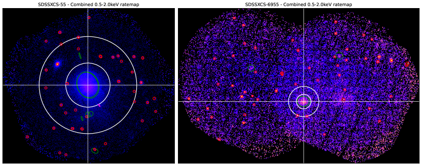
Figure 1: XMM 0.5-2.0 keV stacked ratemaps of SDSSXCS-55 (left) and SDSSXCS-6955 (right), which have been selected to demonstrate our methodology. Point sources are highlighted by red circles and extended sources by green ellipses. The white cross-hair indicates the cluster centroid, and the solid inner and outer while circles indicate the $R_{2500}$ and $R_{500}$ radii respectively (see Table 1 for input values).

2.1 Initiating Xga

Throughout this work, we use public XMM data from the XMM Science Archive that has been pre-processed to produce cleaned event files and region lists. The region lists encode information about the source centroid, size, and shape. All pre-processing used herein relies on the the XCS methodology that is fully described in Lloyd-Davies et al. (2011) and Giles et al. (2022). In brief, the initial EPIC (MOS and PN) data were processed with v14.0.0 of the XMM Science Analysis Software (SAS; Gabriel et al., 2004), using EMCHAIN and EPCHAIN functions to generate event lists. Following this, the event lists were screened for periods of high background and then individual (PN, MOS1, MOS2) and merged (PN+MOS1+MOS2) EPIC images (and corresponding exposure maps) were then generated. All images/maps have a pixel size of 4.35″. Next, X-ray source detection is performed using a custom version of wavdetect (Freeman et al., 2002) called Xapa (for XCS Automated Pipeline Algorithm). Once sources in an image have been located, Xapa classifies them as either point-like or extended sources. Region lists of sources are created for each XMM observation (a given source can appear in multiple region lists if there are overlapping observations). Once all the observations have been processed, a master source list (MSL), with duplicates removed, is generated. To date, 12,582 observations have been processed by XCS, covering 1,068 non-overlapping square degrees of sky, and yielding 400,225 X-ray source detections in the 0.5-2.0 keV band.

In addition to the XCS supplied cleaned event files and region lists, the following information is required to initiate the Xga analysis of a cluster: a coordinate for the cluster centre, the redshift, at least one radius to define the analysis region, and a set of values for the cosmological parameters $\Omega_{M}$, $\Omega_{\Lambda}$, and $H_{0}$. With regard to the cluster centre, this depends on the selection method (e.g. it could be defined by the brightest galaxy, rather than a feature in an X-ray image) and on the analysis method (e.g. it could be defined by the peak of the X-ray surface brightness or by the weighted centroid). Given this ambiguity, we henceforth refer to the user-defined coordinate (or UDC), rather than to the “cluster centre”.

With regard to the analysis region radius, this can be an overdensity radius, e.g. $R_{500}$, or a proper radius with no associated physical significance (e.g. 300 kpc).

For our example clusters, SDSSXCS-55 and SDSSXCS-6955 (and for the analysis presented in Section 4), the UDC${}^{\ref{foot:udc}}$, the redshift, and the analysis region radii ($R_{2500}$, $R_{500}$) were taken from the data tables in Giles et al. (2022). Giles et al. (2022) analysed these clusters using the XCS Post Processing Pipeline (XCS3P). As per Giles et al. (2022), the cosmological parameters were set to $\Omega_{\rm{M}}$=0.3, $\Omega_{\Lambda}$=0.7, and $H_{0}$=70 km s^-1 Mpc^-1.

To ensure all relevant data sets are used during the analysis of a given cluster, Xga explores the full set of XCS processed data to retrieve any XMM observations meeting these criteria; an aimpoint within 30′ of the input UDC${}^{\ref{foot:udc}}$, and >70% of the chosen analysis region falling on active regions of the detectors. Two observations each were retrieved for our example clusters (Table 1), SDSSXCS-55 (0149880101 & 0303930101) and SDSSXCS-6955 (0404965201 & 0677600131).

2.2 Generating image and exposure maps

Once the relevant XMM data have been retrieved, see Section 2.1, Xga generates images, exposure maps, and ratemaps. For this, Xga interfaces with the SAS evselect and eexpmap tools. These images and maps are essential to the derivation of $M_{\rm{hydro}}$ as they are used to generate of surface brightness profiles, which in turn are used to estimate $\rho_{g}(r)$ (see Section 2.7). Images are also useful for inspection throughout the analysis process e.g., to check masked regions (see Section 2.4).

We note that, in principle, the images already existing in the XCS archive (those on which Xapa was run) could have been used by Xga for the analyses herein. However, in practice, generation of fresh images is worthwhile because it simplifies the process of merging multiple observations, and gives additional freedom in the current analysis (e.g., selecting an energy range; XCS only stores images in the 0.5-2.0 keV and 2.0-10.0 keV ranges).

In Figure 1, we show the Xga generated XMM images of our example clusters, SDSSXCS-55 and SDSSXCS-6955; these are the stacked images of every EPIC instrument for every usable observation of the clusters. The Xapa (Section 2.1) defined source regions are overlaid; with red (point source), green (extended source), or magenta (extended source similar in size to the PSF) outlines. The UDC${}^{\ref{foot:udc}}$ is shown with a white cross. The analysis regions ($R_{2500}$ and $R_{500}$) are shown with white solid outlines. Note that, in these examples, two observations have been stacked into a composite image. As each observation has its own source region list, multiple source outlines can sometimes be seen in the overlap regions.

2.3 Automated source masking

As described above (Section 2.1), every XCS processed image has an associated list of detected source regions. Most of these will not be associated with the cluster of interest and need to be masked from both the image files (Section 2.2), used during surface brightness fitting (Section 2.7), and from the cleaned event lists (Section 2.1), used during spectral analysis (Section 2.5). In almost all cases, the only source region not masked by default is the one associated with the cluster of interest (see below for two exceptions). This source is identified as the one containing the location of the UDC${}^{\ref{foot:udc}}$. For the analysis herein, we apply an additional filter: the source must also have been classed as extended by the Xapa pipeline. The black areas in Figure 2 (left) show the region automatically masked for SDSSXCS-55. This figure is a zoom into the $3R_{500}\times 3R_{500}$ region of Figure 1 (left).

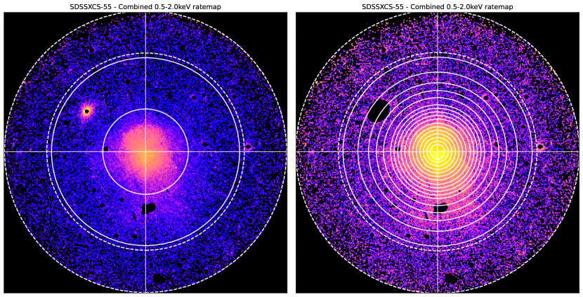
Figure 2: An XMM 0.5-2.0 keV stacked ratemap of SDSSXCS-55. The white cross-hairs indicate the UDC${}^{\ref{foot:udc}}$. Left: The solid inner and outer circles indicate the location of $R_{2500}$ and $R_{500}$ respectively. The dashed annulus indicate 1.05-1.5$R_{500}$ (the background region used in the global spectral analysis, see Section 2.5). An automated mask, to remove contaminating sources identified by xapa has been applied (black areas, see Section 2.3). Right: The default mask has been adjusted by hand to remove more emission from the bright point source in the top left (see Section 2.4). The solid (dashed) circles indicate the source (background) annuli used during the radial spectral fitting used to measure projected temperature profiles (see Sections 2.5 and 2.10).

Below are two exceptions to the masking process detailed above:

• The treatment of Xapa point-like sources detected within 0.15$R_{\rm{analysis}}$ of the cluster centroid. These sources are not masked because Xapa occasionally misidentifies cool cores of clusters as point sources.

• The treatment of overlapping Xapa extended source regions. If the cluster of interest was observed in two or more XMM pointings, then the associated Xapa extended sources may not fully overlap. This is more likely if the observations are offset from each other and/or that have differing exposure times. Therefore, if the respective source centres are within a projected distance of $<R_{500}$ of the input cluster centroid, then none of those source regions are masked.

2.4 Manual data checks

Once the images have been generated (Section 2.2) and the default masks applied (Section 2.3), the next step involves manual intervention via eye-ball checks to i) identify observations that were not suitable for further analysis, ii) increase the size of masked regions if the default mask was not large enough, and iii) add masked regions for sources missed by Xapa. With regard to i), this process is similar to that described in Section 2.3 of Giles et al. (2022). It is used to remove from further analysis observations with abnormally high background levels (e.g. Figure A1(a) of Giles et al., 2022), and those corrupted by a very bright point source (such sources produce artefacts in the XMM images including readout streaks and ghost images of the telescope support structure; e.g. Figure A1(b) of Giles et al., 2022). Of the 457 XMM observations identified as being relevant to the clusters in this paper, 43 were rejected entirely, and 4 had data from one or more (of the 3 EPIC) instruments rejected.

With regard to ii), occasionally the Xapa defined region is not large enough to encapsulate all the emission from a bright point source, or from a neighbouring (but physically distinct) extended source. This can impact subsequent analysis if the source falls in either within $R_{500}$ of the cluster UDC${}^{\ref{foot:udc}}$ or within the background annulus. For the Giles et al. (2022) analysis, this extra masking step was cumbersome and time-consuming. So, in Xga, a GUI was developed that makes it simple to interact with, and modify existing regions. With regard to iii), there is a rare Xapa failure mode whereby it fails to detect some of the sources in a given observation. Using the GUI, it is easy to add new regions if a source or artefact (visible by eye in the image) has been missed by Xapa.

Combined images (all observations and instruments that passed our flare checks) for each of the galaxy clusters in this work were examined, and adjustments to regions were made. We altered or added regions for 60 (40%) of the SDSSRM-XCS sample, 44 (44%) of the XXL-100-GC sample, and 26 (56%) of the LoCuSS High-$L_{\rm{X}}$ sample. Figure 2 (right) shows part of the XMM observation containing SDSSXCS-55. This Figure highlights where a source mask has been expanded from its default (Xapa) size.

2.5 Generating and fitting X-ray spectra

Spectral analysis is essential to the estimation of hydrostatic masses, both for the derivation of $\rho_{g}(r)$ and $T(r)$. In the case of $\rho_{g}(r)$, only a global (cluster wide) spectral analysis is needed, whereas for $T(r)$, spectral analysis in radial bins is required.

For the global spectral analysis of our example clusters, the analysis region (radius and UDC${}^{\ref{foot:udc}}$) is defined by the user as an initiation input to Xga (Section 2.1). A background region also needs to be defined. In the implementation of Xga used herein, the background region is an annulus. For our example clusters, SDSSXCS-55 and SDSSXCS-6955 (and for the analysis presented in Section 4), the inner and outer radii of the annulus are set at 1.05R₅₀₀ and 1.5R₅₀₀ respectively; for $R_{2500}$ measurements they are set at 2$R_{2500}$ and 3$R_{2500}$, and for 300 kpc measurements (for the XXL-100-GC sample, Section 3.1.2) they are set to 3.33$R_{\rm{300~{}kpc}}$ and 5$R_{\rm{300~{}kpc}}$.

For the radial spectral analysis, Xga uses a series of $N$ circular source apertures with increasing radii, out to a user defined outer radius, $R_{\rm{outer}}$ and centered on the UDC${}^{\ref{foot:udc}}$. The innermost aperture is a full circle, the others are annuli. The user defines a minimum annulus width (also the inner circle radius) in arcseconds, $\Delta\theta_{\rm min}$. This minimum is set to account for the PSF of the instrument. For all the cluster analyses herein, we set this to be $\Delta\theta_{\rm min}$=20″ (roughly twice the FWHM of the XMM EPIC-PN on-axis PSF, see Section 2.6). If the specified $R_{\rm{outer}}$ value for a given cluster, when converted to units of arcseconds ($\theta_{\rm{outer}}$), is not an integer multiple of $\Delta\theta_{\rm min}$, it is adjusted (outwards) accordingly, to become $\theta_{\rm{outer}}^{\prime}$. A background region is then defined and used for all the bins. For the radial analysis of our example clusters, SDSSXCS-55 and SDSSXCS-6955 (and the analysis presented in Section 4), it was set to be an annulus of 1.05-1.5 $\theta_{\rm{outer}}^{\prime}$.

The widths of the bins used in the spectral analysis are set through an iterative process. This starts with determining whether $\theta_{\rm{outer}}^{\prime}$ is at least $4\times\Delta\theta_{\rm min}$. If not, then the process stops (because it is not realistic to generate a $T(r)$ profile from less than 4 bins). If it is exactly $4\times\Delta\theta_{\rm min}$, then 4 bins (each of $\theta_{\rm min}$ in width) are used in the analysis. If it is $5\times\Delta\theta_{\rm min}$, then some bins may be expanded (to $2\times\Delta\theta_{\rm min}$, $3\times\Delta\theta_{\rm min}$ etc.) to improve the signal to noise. The width of a given bin expands (inwards) until either a) the user defined minimum number of background subtracted counts is reached, or b) the number of bins drops to 4. The number of bins defined in this way will depend on the quality of the detection and on the $R_{\rm outer}$ (and hence projected size) of the cluster.

The way that the annular spectra are radially binned can have a significant effect on the temperature profiles that are created from them, and different criteria may be used to decide on the binning (see e.g., Chen et al., 2023). The goal is to make the extraction region large enough that sufficient X-ray counts are present to constrain spectral properties (e.g. temperature), whilst maintaining a good spatial resolution.

Achieving a minimum number of counts per spectral annulus is not always sufficient to guarantee a ‘good’ temperature profile. In an effort to mitigate potential issues, we generate two sets of temperature profiles, with different targeted minimum counts per bin (1500 and 3000 counts). As 1500 counts should be sufficient for a well constrained $T_{\rm X}$ value (see Figure 16 in Lloyd-Davies et al., 2011), preference is given to profiles measured from those spectra. However, if there is a problem with the 1500 count-binned temperature profile, we instead use the 3000 count-binned profile. Such problems include:

• The spectral fitting process failing to converge for some annuli. Even if only one annulus failed in this manner, the entire temperature profile is unusable.

• Annular temperature values have very poorly constrained uncertainties, this can make the deprojection process quite unstable, and cause problems when fitting a temperature profile model to the final 3D temperature profile.

• Model fits to the deprojected, three-dimensional, temperature profile resulting in unphysical mass profiles, where the hydrostatic mass radial profile is not monotonically increasing.

For the clusters analysed herein, the number of annular bins varied from $N=4$ (the defined minimum) to $N=22$. For our example clusters, it was $N=17$ and $N=4$ for SDSSXCS-55 and SDSSXCS-6955 respectively.

Once the source and background regions have been defined, spectra are generated for every camera-plus-observation combination (and in each bin for the radial analysis) of the respective galaxy cluster.

For our example clusters, SDSSXCS-55 and SDSSXCS-6955, this corresponds to 6 (132) and 6 (24) spectra respectively for the global (radial) analyses; the annular spectra for this example were generated with a minimum of 1500 counts. Xga uses the SAS evselect tool to create the initial spectra, selecting events with a FLAG value of 0, and a PATTERN of ${\leq}4$ for PN and ${\leq}12$ for MOS data. The SAS specgroup tool is used to re-bin each spectrum so that there is minimum number of counts per channel (in the analysis herein, we set that to be 5, though it can be configured by the user).

The spectral analysis requires response curves (known as ancillary response files; ARFs) to proceed. These are calculated for each spectrum individually. For this, we use a detector map generated with x and y bin sizes set to 200 detector coordinate pixels, and with the same event selection criteria as the spectrum. We preferentially select an image from another instrument, if available, e.g. a PN image for a MOS detector map, and vice versa. This helps to mitigate the effects of chip gaps.

Xga uses xspec (Arnaud, 1996) to fit emission models to the spectra. For the analyses herein, we use an absorbed plasma emission model (constant${\times}$tbabs${\times}$apec; Wilms et al., 2000; Smith et al., 2001). The multiplicative factor represented by constant helps to account for the difference in normalisation between spectra being fitted simultaneously. The $\rm{n_{H}}$ values required by tbabs are retrieved using the HEASoft nh command. The starting metal abundance value ($Z$) is defined by the user. For the analysis herein, $Z=0.3Z_{\odot}$ was used. The redshift is always fixed at the input value during Xga fitting. The $\rm{n_{H}}$ and $Z$ value can be fixed or left free depending on the use case. For our example clusters, SDSSXCS-55 and SDSSXCS-6955, and the analysis in Section 4, they were fixed.

The fits are performed using the $c$-statistic (Cash, 1979) using a methodology described in detail in (Giles et al., 2022, section 3). Note that not all spectra will yield fitted parameters. There are several quality checks in the Giles et al. (2022) method that have been replicated in Xga. If a given spectrum fails one of those checks, then it is removed from the analysis. If all spectra related to a given analysis region are removed in this way, then no spectral parameter fits will be reported by Xga. Spectral fitting results for our two example clusters are shown in Figure 3. Validation tests of the Xga spectral fitting process can be found in Section 3.

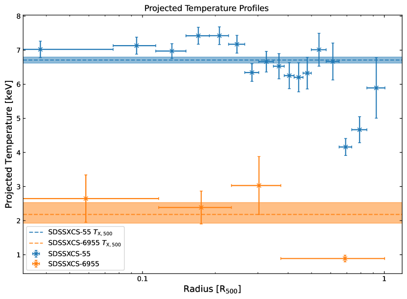
Figure 3: Projected temperature profile measurements for the demonstration clusters, SDSSXCS-55 (blue; upper points) and SDSSXCS-6955 (orange; lower points). Temperatures are plotted against the central radii of the annuli they were measured within. The global temperature values measured by Xga within $R_{500}$ for each cluster is indicated by horizontal lines, with the shaded region representing 1$\sigma$ uncertainty.

2.6 Correcting images for PSF distortion

The XMM EPIC-PN on-axis PSF has a full width half maximum of ${\sim}12.5\arcsec$ (XMM-Newton SOC et al., 2022), and the EPIC-MOS1 and MOS2 camera on-axis PSFs have a FWHM of ${\sim}4.3\arcsec$. The PSF of all three EPIC cameras changes size and shape depending on the position on the detector, with the PSF causing stretching of bright sources along the azimuthal direction (e.g. Read et al., 2011; XMM-Newton SOC et al., 2022). Therefore, Xga has been configured to make a PSF correction to XMM images. These corrections are important to our goal of estimating $M_{\rm hydro}$ because the $\rho(r)$ profiles rely on surface brightness maps (see Section 2.7). The PSF correction approach deployed in Xga uses the Richardson-Lucy algorithm (Richardson, 1972; Lucy, 1974) combined with the ELLBETA XMM PSF model. As the XMM PSFs vary with position, the de-convolution is carried out separately in a user defined grid across the image. For the analysis here in, we used a $10\times 10$ grid. Figure 4 shows a comparison of the pre and post PSF correction combined count-rate maps for our two example clusters.

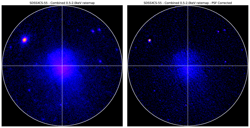
Figure 4: A demonstration of the image PSF correction capabilities of Xga. The white cross-hair indicates the UDC${}^{\ref{foot:udc}}$ of SDSSXCS-55. The white circle indicates the $R_{500}$ aperture centered on the UDC${}^{\ref{foot:udc}}$. Both images show the $2R_{500}\times 2R_{500}$ region. Left: the combined RateMap before PSF correction. Right: After PSF correction. Note, individual camera images were corrected separately, and then stacked.

2.7 Generating surface brightness and emissivity profiles

Xga can be used to construct radial surface brightness (SB) profiles from combined (Section 2.2) PSF corrected (Section 2.6) ratemaps. For this, the region (radius and centre) over which the SB is determined is defined by the user as an initiation input to Xga (Section 2.1). A background region also needs to be defined. In Xga, the background region is an annulus. For our example clusters, SDSSXCS-55 and SDSSXCS-6955 (and for the analysis presented in Section 4), the inner and outer radii were set at 1.05$R_{500}$ and 1.5$R_{500}$ respectively. Other sources in the respective XMM combined ratemaps were removed prior to profile generation using the automated and Xga generated masks (see Sections 2.3, and 2.4). For the analyses herein (unless otherwise stated), we used the default Xga settings radial bins of width 1 pixel (4.35″) and an energy range of 0.5-2.0 keV. The uncertainties on the background-subtracted SB profile are calculated by assuming Poisson errors on the counts in each annulus. Figure 5 shows cluster surface-brightness profiles for SDSSXCS-55 and SDSSXCS-6955.

The SB profiles are projected quantities and are in instrument specific units (i.e. detected photons per second per unit area). The next step toward our goal of measuring a $\rho(r)$ profile is to de-project them and to infer a three-dimensional profile (i.e. emitted photons per second per volume). As the true 3D distribution of ICM electrons is unknown, we have to rely on a model for the de-projection. Fitting to radial profiles using Xga is described in Appendix A. We use the beta model throughout this work, but other models are available in Xga. This model takes the form:

$$S_{X}(R)=S_{0}\left(1+\left(\dfrac{R}{R_{c}}\right)^{2}\right)^{-3\beta+0.5},$$ (2)

where $S_{0}$ is a normalisation factor, $R_{c}$ is the radius of the core region and $\beta$ is the slope outside the core region. Parameter priors used during this work can be found in Table 4. An advantage of the beta model is that there is an analytical solution for the inverse-abel transform which is used to deproject it from a 2D to a 3D profile, making the assumption of spherical symmetry. This results in a 3D radial volume emissivity profile $\epsilon(R)$.

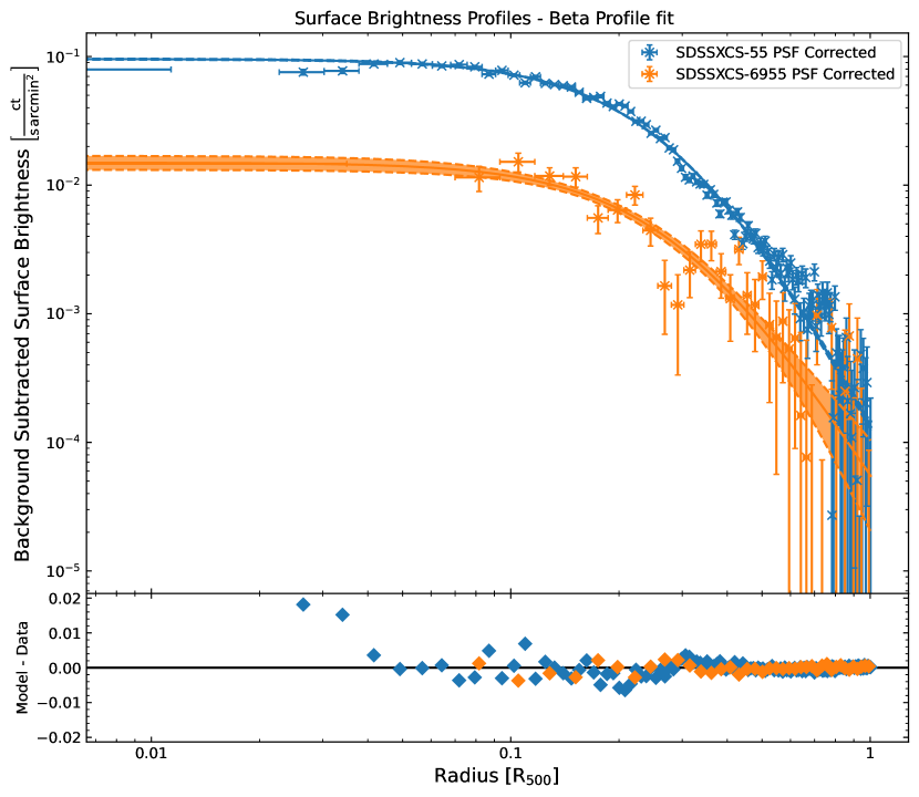
Figure 5: Surface brightness profiles (constructed from images in the 0.5-2.0 keV band) generated by Xga for SDSSXCS-55 (blue; upper points) and SDSSXCS-6955 (orange; lower points), with the spatial binning set to one pixel (4.35″). Residuals to the fit to a beta model are shown in the bottom panel.

2.8 Generating density profiles

With the emissivity profiles in hand, the next task is to convert them to gas density profiles. For this we use of the definition of the APEC emission model normalisation,

$$N_{\texttt{APEC}}=\dfrac{10^{-14}}{4\pi(D_{A}(1+z))^{2}}\int n_{e}n_{p}dV,$$ (3)

where $N_{\texttt{APEC}}$ is the normalisation of the APEC plasma emission model (in units of $\rm{cm}^{-5}$), $D_{A}$ is the angular diameter distance to the cluster (in units of cm), $z$ is the redshift of the cluster, $n_{e}$ and $n_{p}$ are the electron and proton number densities (in units of $\rm{cm}^{-3}$).

To make use of Equation 3, we need to calculate a conversion factor, $K_{N}$, between $N_{\texttt{APEC}}$ and XMM count-rate ($C_{r}$), where $N_{\texttt{APEC}}=K_{N}C_{r}$. To calculate $K_{N}$, we implement an Xga interface to the xspec tool FakeIt, which can be used to simulate spectra given an emission model and an instrument response. This is used to generate simulated spectra for every camera-plus-observation combination (using ARFs and RMFs extracted at the UDC${}^{\ref{foot:udc}}$ during the generation of spectra, see Section 2.5). The simulations are performed using an APEC model absorbed with tbabs. The ${\rm n}_{\rm H}$ value for tbabs is set to the HI4PI Collaboration et al. (2016) value for that cluster. The spectra are simulated with a normalisation fixed at 1, a fixed global temperature measured for that cluster (within $R_{500}$ for LoCuSS High-$L_{\rm{X}}$/SDSSRM-XCS, within 300 kpc for XXL-100-GC), a metallicity of 0.3 $Z_{\odot}$, and the input redshift of the cluster. The simulated spectra are all ‘observed’ for a set exposure time of 10 ks, and are used to measure count-rates in the 0.5-2.0 keV band, which corresponds to the energy range of the ratemaps used to generate SB profiles. The count-rates for each instrument of each observation are then weighted by the average effective area between 0.5-2.0 keV (drawn from the corresponding ARF) and combined into a single conversion factor $K_{N}$. This conversion factor is suitable for use with emissivity profiles generated from combined ratemaps.

This conversion factor, $K_{N}$, allows Equation 3 to be written in terms of the 3D emissivity $\epsilon(R)={C_{r}(R)}{V}^{-1}$, and the product of the electron and proton number densities $n_{e}n_{p}$ (which we can use to calculate the total gas density),

$$n_{e}(R)n_{p}(R)=\dfrac{4\pi K_{N}(D_{A}(1+z))^{2}\epsilon(R)}{10^{-14}}.$$ (4)

At this point we assume the ratio of electrons to protons in the intra-cluster medium, given by $n_{e}=R_{ep}\times n_{p}$, which substituted into Equation 4, gives an expression for $n_{p}$ of

$$n_{p}(R)=\sqrt{\dfrac{4\pi K_{N}(D_{A}(1+z))^{2}\epsilon(R)}{R_{ep}10^{-14}}}.$$ (5)

We choose to use the solar abundances presented in Anders & Grevesse (1989) to calculate this ratio, $R_{ep}=1.199$. The total gas number density, $n_{g}=n_{e}+n_{p}=(1+R_{ep})n_{p}$, is thus calculated using the expression for $n_{p}$ from Equation 5.

At this point the mean molecular weight $\mu=0.61$ and the atomic mass unit are used to convert number density to mass density. Thus, we calculate gas density from emissivity with quantities that we can measure, or already know;

$$\rho_{\rm{gas}}(R)=\mu m_{u}(1+R_{ep})\sqrt{\dfrac{4\pi K_{N}\epsilon(R)(D_{A}(1+z))^{2}}{R_{ep}10^{-14}}}.$$ (6)

Once the radial gas density profile is measured using Equation 6, we use the fitting functionality discussed in Appendix A to fit a parametric model to the resulting data points. Density profiles for SDSSXCS-55 and SDSSXCS-6955 are shown in Figure 6.

2.9 Measuring gas masses

Once a gas density profile (Equation 6) has been derived, we can use it to measure total gas masses within given radii. This is achieved through a spherical volume integral,

$$M_{\rm{gas}}(<R_{\Delta})=4\pi\int_{0}^{R_{\Delta}}\rho_{\rm{gas}}(R)R^{2}dR,$$ (7)

and can be used to measure both total gas masses within particular radii (e.g. $R_{500}$), or to create cumulative gas mass profiles.

It is desirable to account for all significant sources of uncertainty in the calculation of gas masses. One source of uncertainty is that on the overdensity radii within which gas mass is measured, which is not accounted for in our measurement of the density profile. Therefore, we have added an optional mechanism to account for uncertainty in the physical radius (e.g. $R_{500}$) when calculating gas mass. For this, we assume a Gaussian posterior distribution for the radius, with the mean being the published value and the standard deviation being the published error. This radius distribution is sampled along with the model posterior distributions to create a gas mass measurement distribution, with the sampled radius for each combination of sampled model parameters acting as the outer radius within which the integral is evaluated. We have applied this method in Section 3.2.2 where we compare Xga and Eckert et al. (2016) gas mass estimates for the XXL-100-GC sample. This is due to the fact that the gas masses measured in Eckert et al. (2016) also account for overdensity radius uncertainty in their analysis. We also use it in Section 4 when generating new $M_{\rm{hydro}}$ estimates for SDSSRM-XCS clusters.

To demonstrate the effect of including the uncertainty on the input radius, the measured gas mass for SDSSXCS-6955 within $R_{500}$ ($669.0^{+62.0}_{-47.9}$ kpc; see Table 1) is $M^{\rm{gas}}_{500}=1.155^{+0.027}_{-0.027}$ $10^{12}\>\rm{M}_{\odot}$ excluding the uncertainty on $R_{500}$, and $M^{\rm{gas}}_{500}=1.153^{+0.089}_{-0.095}$ $10^{12}\>\rm{M}_{\odot}$ including the $R_{500}$ uncertainty. We can see that the gas mass uncertainties, when we account for radius uncertainty, are ${\sim}3$ times larger than when we don’t.

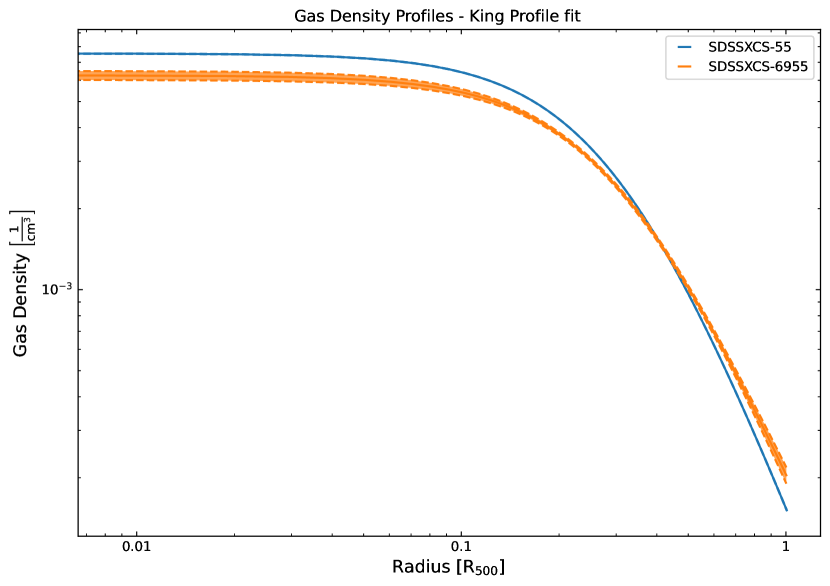
Figure 6: Gas density models generated by Xga for SDSSXCS-55 (blue) and SDSSXCS-6955 (orange). These are determined from the model fits to surface-brightness profiles shown in Figure 5.

2.10 Generating 3D temperature profiles

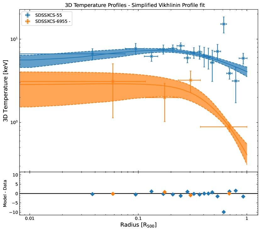
Figure 7: Three-dimensional temperature profiles, de-projected from the temperature profiles shown in Figure 3, for SDSSXCS-55 (blue points) and SDSSXCS-6955 (orange points). Fits to the temperature profiles using the simplified Vikhlinin model in Equation 10, using the process outlined in Appendix A, are given by the blue (SDSSXCS-55) and orange (SDSSXCS-55) solid lines. For each fit, the shaded regions, bounded by the dashed lines, represent the 1$\sigma$ uncertainty. Residuals to the fit are shown in the bottom panel.

The second property we must measure to calculate a cluster’s hydrostatic mass is the three-dimensional temperature profile. The radial spectral analysis described in Section 2.5 results in a set of projected temperature measurements (one for each of the $N$ radial bins). Each projected temperature is a weighted combination of the temperatures in the three-dimensional shells of the cluster that the annulus intersects with. To recover the 3D distribution, $T(r)$, we opt to use the ‘onion-peeling’ method (see descriptions in e.g., Ettori et al., 2002; Ghirardini et al., 2018). First, the volume intersections between the analysis annuli (projected back into the sky) and the spherical shells which we separate each cluster into (defined as having the same radii as the annuli) must be calculated. The volume intersections can be calculated (see Appendix A of McLaughlin, 1999) as,

$$\begin{split}\bm{V}_{\rm{int}}=\frac{4\pi}{3}\big{[}&max\{0,(\bm{R}_{\rm{so}}^{2}-\bm{R}_{\rm{ao}}^{2})^{\frac{3}{2}}\}-max\{0,(\bm{R}_{\rm{so}}^{2}-\bm{R}_{\rm{ao}}^{2})^{\frac{3}{2}}\}+\\ &max\{0,(\bm{R}_{\rm{si}}^{2}-\bm{R}_{\rm{ao}}^{2})^{\frac{3}{2}}\}-max\{0,(\bm{R}_{\rm{si}}^{2}-\bm{R}_{\rm{ai}}^{2})^{\frac{3}{2}}\}\big{]},\end{split}$$ (8)

where $\bm{R}_{\rm{so}}$ is the matrix of shell outer radii, $\bm{R}_{\rm{ao}}$ is the matrix of annulus outer radii, $\bm{R}_{\rm{si}}$ is the matrix of shell inner radii, and $\bm{R}_{\rm{ai}}$ is the matrix of annulus inner radii. The $\bm{V}_{\rm{int}}$ matrix is a two dimensional matrix describing volume intersections between all combinations of annuli and three-dimensional shells.

Second, an emission measure profile is calculated using the APEC Normalisation 1D profile produced during the spectral fitting of the set of annular spectra. This calculation uses Equation 3 and rearranges to solve for the integral. As the projected temperature measured within a given annulus is a weighted combination of the shell temperatures intersected by that annulus, we can infer the temperature of a shell (for past usage see Ghirardini et al., 2018) with

$$\bm{T}_{\rm{shell}}=\dfrac{(\bm{V}_{\rm{int}}^{\rm{T}})^{-1}\times\bm{T}_{\rm{annulus}}\rm{\textbf{EM}}}{(\bm{V}_{\rm{int}}^{\rm{T}})^{-1}\times\rm{\textbf{EM}}}.$$ (9)

$\bm{T}_{\rm{shell}}$ is the matrix of spherical shell temperatures that we aim to calculate, $\bm{V}_{\rm{int}}$ is the matrix of volume intersections between all combinations of annuli and shells (see Equation 8), EM is the emission measure matrix, and $\bm{T}_{\rm{annulus}}$ is the projected temperature matrix; $\times$ represents the matrix product. We propagate the uncertainties from the projected temperature and emission measure profiles by generating 10000 realisations of each profile, assuming Gaussian errors on each data point. We then use the profile realisations to calculate 10000 instances of the deprojected temperature profile. These distributions are used to measure 90% confidence limits on each deprojected temperature data point.

Once three-dimensional, de-projected, gas temperature profiles have been measured, we use the methods discussed in Section A to model the profiles with a simplified version of the Vikhlinin et al. (2006) temperature model as detailed in Ghirardini et al. (2018). The use of the simplified model allows for the modelling of temperature profiles with fewer temperature bins (due to the use of less free parameters). This temperature profile takes the form:

$$T_{3D}(r)=\dfrac{T_{0}\left(\left(\frac{r}{r_{\rm cool}}\right)+\frac{T_{\rm min}}{T_{0}}\right)\left(\frac{r^{2}}{r_{t}^{2}}+1\right)^{-\frac{c}{2}}}{\left(\frac{r}{r_{\rm cool}}\right)^{a_{\rm cool}}+1},$$ (10)

where $T_{0}$ is a normalisation factor, $T_{\rm min}$ is the minimum temperature, $r_{\rm cool}$ is the radius of the cool central region, $a_{\rm cool}$ is the slope of the cool region out to a radius $r_{\rm cool}$, c is the slope at large radii occurring at a transition radius $r_{t}$. Parameter priors can be found in Table 4. Figure 7 shows three-dimensional temperature profiles for clusters SDSSXCS-55 and SDSSXCS-6955, along with the corresponding 1$\sigma$ uncertainty (given by the shaded regions).

2.11 Generating hydrostatic mass profiles

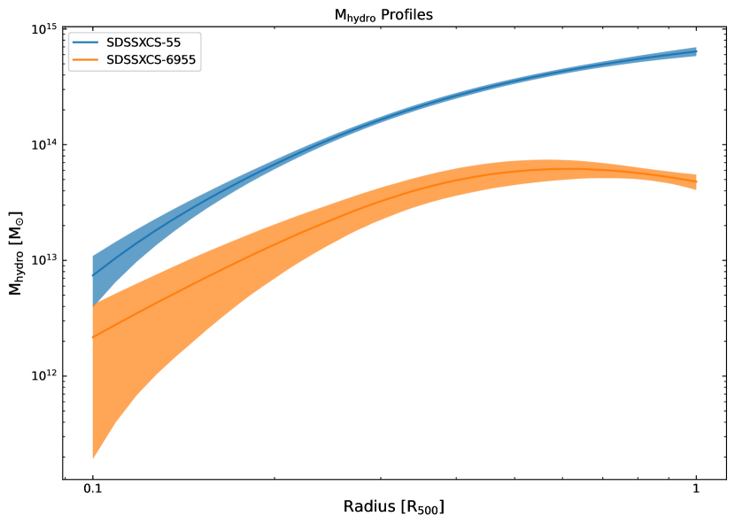
Figure 8: An example hydrostatic mass profile generated for SDSSXCS-55. This profile was generated using the model fits to the density profile shown in Figure 6, and the temperature profile shown in Figure 7.

Once we have measured a 3D radial gas density profile (details in Section 2.8) and a 3D radial temperature profile (details in Section 2.10), we can use Equation 1 to measure hydrostatic masses. As such, Xga creates hydrostatic mass profiles as a function of radius (e.g. Figure 8). The hydrostatic mass equation not only involves the temperature and density profile values at each radius for which a enclosed mass is measured, but also the derivatives of those profiles with respect to radius. The king profile and temperature profiles both have analytical first-derivatives, and as such these are used to calculate the slope at a given radius, rather than a numerical approximation.

Xga models can return posterior distributions of the value of the model (or model slope) at a given radius, rather than a single value. This is based on drawing randomly from the parameter posterior distributions found from the fitting process described in Section A. When calculating a hydrostatic mass at a specified radius, the temperature and density parametric models generate 10000 realisations of themselves; these realisations are then used to retrieve absolute values of $T_{\rm{3D}}$ and $\rho_{\rm{g}}$ at the specified radius, as well as $\frac{dT_{\rm{3D}}}{dr}$ and $\frac{d\rho_{\rm{g}}}{dr}$ values. As such a distribution of hydrostatic mass measurements is created for the given radius, and 90% confidence limits are calculated.

We also implement an optional method of propagating errors on the chosen radius, to help account for uncertainties on the overdensity radii which masses are commonly calculated within. This is akin to the optional step implemented for the calculation of Xga gas masses at the end of Section 2.9. When an uncertainty is provided along with a radius, we assume a Gaussian distribution and draw 10000 random radii. Then, when the profile realisations are generated and a distribution of hydrostatic masses are measured, the randomly drawn radii are used rather than a fixed value. Distributions are generated for absolute values and derivatives can all take radius uncertainties into account. This is not used in our comparisons to LoCuSS $M_{\rm{hydro}}$ measurements in Section 3.2.3, as radius uncertainties were not published by Martino et al. (2014). We do include radius uncertainties in our calculation of SDSSRM-XCS cluster masses presented in Section 4. Mass profiles for the clusters SDSSXCS-55 and SDSSXCS-6955, along with the corresponding 1$\sigma$ uncertainty (given by the shaded regions), are shown in Figure 8.

3 Validation Tests

We have tested the validity of the Xga approach described in Section 2 by comparing the Xga outputs to those presented in the literature. For this we have used three different cluster samples. The samples used for validation are described in Section 3.1. In Sections 3.2.1, 3.2.2, 3.2.3 we compare the Xga measurements of $T_{\rm X}$, $M_{\rm{gas}}$, $M_{\rm{hydro}}$ respectively to literature values.

Table 2: Summaries of the literature galaxy cluster samples used in this work (see Section 3) to validate the Xga methodology.

Sample Name	NCL, $z$	Brief description
SDSSRM-XCS	150, $0.1{<}z{<}0.35$	SDSS redMaPPer clusters (Rykoff et al., 2014) with available XMM observations. Section 3 presents a comparison to results presented in Giles et al. (2022).
XXL-100-GC	99, $0.05<z<0.9$	Drawn from a sample of the 100 X-ray brightest clusters in the XXL survey regions (Pierre et al., 2016; Pacaud et al., 2016). Section 3 presents a comparison to results presented in Giles et al. (2016) and Eckert et al. (2016).
LoCuSS High-$L_{\rm{X}}$ (a)	33, $0.15<z<0.3$	Drawn from clusters detected in the the ROSAT All Sky Survey (Ebeling et al., 2000). The sample contains 50 clusters satisfying the following conditions; ${\rm n}_{\rm H}<7\times 10^{20}$ cm2, $-25^{\circ}<\delta<65^{\circ}$ and $L_{X}[0.1-2.4~{}{\rm keV}]E(z)^{-2.7}\geq 4.2\times 10^{44}$ erg s-1. All clusters have subsequent observations by XMM or Chandra. Section 3 presents a comparison to 33 clusters with XMM derived results presented in Martino et al. (2014).
LoCuSS High-$L_{\rm{X}}$ (b)	32, $0.15<z<0.3$	As above, but for clusters satisfying $L_{X}[0.1-2.4~{}{\rm keV}]E(z)^{-1}\geq 4.4\times 10^{44}$ erg s-1 between $0.15<z<0.24$, and $L_{X}[0.1-2.4~{}{\rm keV}]E(z)^{-1}\geq 7.0\times 10^{44}$ erg s-1 between $0.24<z<0.3$. Resulting in a sample of 41 clusters. Section 3 presents a comparison to 32 clusters with XMM derived results presented in Mulroy et al. (2019).

3.1 Validation Samples

The validation samples are SDSSRM-XCS (Giles et al., 2022), XXL-100-GC (Pacaud et al., 2016), and LoCuSS High-$L_{\rm{X}}$ (Martino et al., 2014). The properties of the validation samples are summarised in Table 2. We note that although both XMM and Chandra based measurements are presented in Martino et al. (2014), we only make comparisons here with XMM, given the known discrepancy between XMM and Chandra derived temperature estimates (e.g., Schellenberger et al., 2015). Excluding duplicates, a total of 268 clusters have been used in the validation tests presented below. Duplicate clusters were identified by cross-matching the samples; to be considered a match, two sources needed to be within a projected distance of 500 kpc (at the cluster redshift) and with $\lvert\Delta z\rvert\leq 0.05$. For each test, we adjusted the Xga initiation values (Section 2.1) to follow those used in the published works as closely as possible (see Sections 3.1.1, 3.1.2, 3.1.3). A companion GitHub repository (see Appendix B for a summary of the structure and contents) contains the exact sample files used in this section.

3.1.1 SDSSRM-XCS

We have used Xga to re-analyse a sample of 150 clusters presented in Giles et al. (2022, hereafter G22). These clusters are referred to as the SDSSRM-XCS$T_{\rm X,vol}$ sub-sample in G22 (see Table 2 therein), but hereafter will be referred to as SDSSRM-XCS for simplicity. The SDSSRM-XCS clusters in the sample were originally selected from SDSS photometry using the redMaPPer (RM) algorithm (Rykoff et al., 2014). The 150 SDSSRM-XCS clusters represent the subset of the original $\simeq$66,000 SDSSRM cluster catalogue that meet the following criteria: they lie within the footprint of the the XMM archive, were successfully processed by the XCS imaging and spectroscopic pipelines ($\Delta T_{\rm X}<25\%$), and have redshifts in the range $0.1<z<0.35$.

The following elements are in common between G22 and our analysis of the SDSSRM-XCS clusters:

• The cosmological model; flat $\Lambda$CDM, assuming $\Omega_{\rm{M}}$=0.3, $\Omega_{\Lambda}$=0.7, and $\rm{H}_{0}$=70 km s^-1 Mpc^-1.

• The XMM data reduction, image generation, and source detection (Section 2.1). This was performed outside of Xga, exactly following the G22 approach. This meant that the automatically masked regions (Section 2.3) were the same in both analyses.

• The UDCs${}^{\ref{foot:udc}}$, redshifts, $R_{500}$, and $R_{2500}$ values. Therefore, the source apertures, and the background annuli (either 1.05-1.5$R_{500}$ or 2-3$R_{2500}$) were the same (i.e. size, shape, and location) during the global spectral fits (Section 2.5), and construction of surface brightness profiles (Section 2.7).

• The model used during the xspec fits. Both analyses used an absorbed APEC plasma model with the column density, redshift, and metal abundance fixed during the fit.

Differences include:

• The choice of manually adjusted source masks and excluded XMM observations (Section 2.4).

• Different versions of certain software packages; G22 used SAS v14.0.0 and xspec v12.10.1f, whereas this work uses SAS v18.0.0 and xspec v12.11.0.

• The pipeline used for the global spectral analysis (there was no radial spectral analysis G22). Herein we use Xga, whereas G22 used XCS3P. One important difference between the two pipelines is the treatment of XMM sub-exposures. Some XMM observations contain multiple sub-exposures by the same instruments. The analyses performed by Xga only make use of the longest individual sub-exposure for a particular instrument of a particular observation, whereas XCS3P makes use of all of the sub-exposures.

3.1.2 XXL-100-GC

We used Xga to re-analyse 99 of the 100 clusters first described in Pacaud et al. (2016). The cluster XLSSC-504 was excluded to be consistent with the Giles et al. (2016) study. A further two clusters were excluded as they did not successfully pass Xga data quality checks: backscale errors were encountered during spectral generation for XLSSC-11, and, for XLSSC-527, no observation fulfils the Xga criterion that the 300 kpc coverage (Section 2.1) fraction should be $>70\%$. We compare the Xga derived global temperature measurements of the remaining 97 to those presented in Giles et al. (2016), and the Xga derived gas mass measurements to those presented in Eckert et al. (2016).

Our analysis of the XXL-100-GC clusters included these elements in common with the published works:

• The cosmological model: $\Omega_{\rm{M}}$=0.28, $\Omega_{\Lambda}$=0.72, and $H_{0}$=70 km s^-1 Mpc^-1, the WMAP9 results (Hinshaw et al., 2013).

• The UDCs${}^{\ref{foot:udc}}$, redshifts, and analysis regions ($r=300$ kpc) of the clusters. Therefore, the source apertures were the same (i.e. size, shape, and location) during the global spectral fits (Section 2.5), and construction of surface brightness (SB) profiles (Section 2.7) of both analyses.

• The model used during the xspec fits was the same. Both analyses used an absorbed APEC plasma model with the column density, redshift, and metal abundance fixed (at 0.3 $Z_{\odot}$, using Anders & Grevesse (1989) abundance tables) during the fit.

• xspec fitting within an energy range of 0.4-7.0 keV.

• Surface brightness profiles were derived from images generated in the 0.5–2.0keV energy band.

• Surface brightness profiles are generated out to $1.2R_{500}$.

• The global temperature value from Giles et al. (2016, $T_{\rm{X}}^{300\rm{kpc}}$) was used for the conversion from SB to emission measure (see Section 2.7).

• $M_{\rm gas}$ values, and errors, were estimated within R₅₀₀ taken from Eckert et al. (2016). Additionally, $M_{\rm gas}$ uncertainties include the error on R₅₀₀ as performed in Eckert et al. (2016), see Section 2.9.

Differences include:

• The input XMM observations. Our analysis includes some XMM observations that entered the archive after the publication of Giles et al. (2016).

• The approach to background subtraction for the global spectral analyses. We used a local, in field, subtraction technique with an annulus of width $1.05-1.5R_{500}$ centered on the UDC${}^{\ref{foot:udc}}$. By comparison, Giles et al. (2016), used either: (i) an annulus centered on the aimpoint of the XMM observation, with a width determined by the diameter of the analysis region of the galaxy cluster (see Figure 1 of Giles et al., 2016); or (ii) an annulus centered on the cluster centroid with an inner radius equal to the extent of the cluster emission and an outer radius a factor 2$\times$ the inner radius.

• The approach to background subtraction used during the generation of surface brightness (and thus emission measure) profiles. Whereas we used a simple technique (see above), Eckert et al. (2016) used a model for the non-X-ray background and a spatial fit for the X-ray background (see section 2.2 and 2.3 in Eckert et al. (2016) for more detail).

• The choice of manually adjusted source masks and excluded XMM observations (Section 2.4).

• Different versions of certain software packages. Pacaud et al. (2016) used SAS v10.0.2, whereas we use SAS v18.0.0. Giles et al. (2016) used xspec v12.8.1i, whereas we use v12.11.0.

• The pipelines used to generate the various analysis products required to obtain $T_{\rm X}$ and $M_{\rm gas}(<r)$ estimates. Herein, we use Xga (Section 2), which differs in several ways to those used in Pacaud et al. (2016), Giles et al. (2016), and/or Eckert et al. (2016).

3.1.3 LoCuSS High-$L_{\rm{X}}$ (a)

We have used Xga to analyse the 33 LoCuSS clusters presented in Martino et al. (2014), for which their gas and hydrostatic masses are determined using only XMM observations. These clusters form the first LoCuSS validation sample, referred to as LoCuSS High-$L_{\rm{X}}$ (a). The full sample definition is given in Table 2. We note that we do not measure any results for ‘RXCJ1212.3-1816’, as its sole XMM observation (0652010201) was excluded during the inspection detailed in Section 2.4 due to residual flaring. Our analysis of the LoCuSS High-$L_{\rm{X}}$ clusters included these elements in common with the published works:

• The cosmological model: flat $\Lambda$CDM, assuming $\Omega_{\rm{M}}$=0.3, $\Omega_{\Lambda}$=0.7, and $\rm{H}_{0}$=70 km s^-1 Mpc^-1.

• The UDCs${}^{\ref{foot:udc}}$ (i.e. choice of cluster centroid locations) and redshifts values were taken from Martino et al. (2014). To compare gas and hydrostatic masses, we used the R₅₀₀ values given in Martino et al. (2014). Therefore, the source apertures were the same (i.e. size, shape, and location) in the relevant aspects (global spectral fits, Section 2.5) of both analyses.

• The model used during the xspec fits was the same. The LoCuSS High-$L_{\rm{X}}$ (a) analyses used an absorbed APEC plasma model with the column density and redshift fixed during the fit. The metallicity is left free to vary. One small difference is that Martino et al. (2014) uses the wabs model (rather than tbabs) to account for absorption.

• We perform xspec fits within an energy range of 0.7-10.0 keV.

• Surface brightness profiles were derived from images generated in the 0.5–2.5 keV energy band.

• Temperature profiles were constructed with a minimum number of background subtracted counts per annulus of 3000.

• Global temperature values were measured from core-excised (0.15-1$R_{500}$) spectra.

• Errors on the gas masses do not include overdensity radius uncertainties (see Sect. 2.9) as Martino et al. (2014) did not use this approach in their analysis.

Differences include:

• The input XMM observations. Our analysis includes XMM observations that entered the archive after the publication of Martino et al. (2014).

• The choice of manually adjusted source masks and excluded XMM observations (Section 2.4).

• The approach to background subtraction. Whereas we used a simple, in field, subtraction technique with an annulus of width $1.05-1.5R_{500}$ (1.05-1.5 $\theta_{\rm{outer}}^{\prime}$) centered on the UDC${}^{\ref{foot:udc}}$, for the global spectral and surface brightness (radial spectral) analyses, Martino et al. (2014), used a spectral modelling approach (see section 3.3.1 and 3.3.3 in Martino et al. (2014) for more detail).

• Different versions of certain software packages; the Martino et al. (2014) work uses SAS v11.0.0, we use SAS v18.0.0. It is not stated which version of xspec was used by Martino et al. (2014), but it will be a considerably older version than we use (v12.11.0).

• The pipelines used to generate the various analysis products required to obtain $M_{\rm gas}(<r)$ and $M_{\rm hydro}(<r)$ estimates. Herein, we use Xga (Section 2), which differs in several ways to those used in Martino et al. (2014).

• The equations to model the density and 3D temperature profiles differ between those used in this work (Equation 4 and Equation 4 for density and temperature respectively) and the form used in Martino et al. (2014, see their Equation 4 and 5 for density and temperature respectively).

3.1.4 LoCuSS High-$L_{\rm{X}}$ (b)

A modified version of the LoCuSS sample selection is given in Mulroy et al. (2019), for which 32 clusters were analysed using only XMM observations to provide global temperature measurements. These clusters form the second LoCuSS validation sample, referred to as LoCuSS High-$L_{\rm{X}}$ (b). The full sample definition is given in Table 2. As the Mulroy et al. (2019) is based largely upon the same analysis as Martino et al. (2014), many of the similarities and differences are the same as those given in Section 3.1.3. However, those specific to LoCuSS High-$L_{\rm{X}}$ (b) are given below. The elements in common include:

• To compare global temperatures, we used the same R₅₀₀ value as that used in Mulroy et al. (2019). The R₅₀₀ values were estimated from the weak lensing analysis outlined in Okabe & Smith (2016).

Differences include:

• Specific information regarding the background subtraction methods used to derive the global $T_{\rm X}$ values provided in Mulroy et al. (2019) is not given, but we assume the same (spectral modelling) approach was used as that detailed in Martino et al. (2014).

3.2 Validation of derived properties

Table 3: Best fit parameters of fixed-slope power-law models fit to comparisons between original published properties of the validation samples (see Section 3.1), and the Xga derived properties. The first column indicates the property compared, the second the particular sample (either SDSSRM-XCS, XXL, or LoCuSS High-$L_{\rm{X}}$(a) and (b)), the third and forth columns gives the best-fit normalisation and intrinsic scatter (with uncertainties) respectively, and the last column links to the relevant figure.

Property	Sample	Norm	Scatter	Figure
		$A$	$\sigma_{\rm int}$
$T_{\rm{X}}^{2500}$	SDSSRM-XCS	0.99$\pm$0.01	0.02$\pm$0.01	9(a)
$T_{\rm{X}}^{500}$	SDSSRM-XCS	1.00$\pm$0.01	0.04$\pm$0.01	9(b)
$T_{\rm{X}}^{\rm 300kpc}$	XXL-100-GC	0.99$\pm$0.01	0.04$\pm$0.01	10
$T_{\rm{X}}^{\rm 500ce}$	LoCuSS High-$L_{\rm{X}}$(b)	1.01$\pm$0.01	0.04$\pm$0.01	11
$M_{\rm{gas}}^{500}$	XXL-100-GC	0.89$\pm$0.06	0.59$\pm$0.05	12
$M_{\rm{gas}}^{2500}$	LoCuSS High-$L_{\rm{X}}$(a)	0.97$\pm$0.02	0.08$\pm$0.01	13(a)
$M_{\rm{gas}}^{500}$	LoCuSS High-$L_{\rm{X}}$(a)	0.93$\pm$0.02	0.13$\pm$0.02	13(b)
$M_{\rm{hy}}^{2500}$	LoCuSS High-$L_{\rm{X}}$(a)	1.10$\pm$0.03	0.08$\pm$0.03	14(b)
$M_{\rm{hy}}^{500}$	LoCuSS High-$L_{\rm{X}}$(a)	1.19$\pm$0.07	0.24$\pm$0.05	14(b)

The validation of the derived properties takes the form of one-to-one (1:1) comparisons to the validation sample described above, and are quantified by fitting a power-law with the slope fixed at unity. The fits were performed in log space using the R package LInear Regression in Astronomy(lira, Sereno, 2016a), fully described in Sereno (2016b). The validations are visualised via 1:1 plots for each property compared, and in each case the best-fit is given by a light-blue solid line and the 68% confidence interval by the light-blue shaded region. The 1, 2 and 3-$\sigma$ intrinsic scatter is given by the grey shaded regions. A summary of fit results can be found in Table 3. In the following sections we discuss the comparisons of each property for each sample in more detail. The results can be reproduced using public Jupyter notebooks

3.2.1 Validation of Xga derived global $T_{\rm X}$ values

SDSSRM-XCS: The temperature comparison is shown in Figure 9 for both the $R_{2500}$ (a) and $R_{500}$ (b) apertures. The best-fit normalisations are 0.99$\pm$0.00 and 1.00$\pm$0.01 for $T_{\rm X}^{500}$ and $T_{\rm X}^{2500}$ respectively. This highlights that the Xga and G22 values are in excellent agreement. This is expected, given the similarities in the input data and the methodology. There is some small amount of scatter around the 1:1 relation, which can be attributed to the small differences in the method (see Section 3.1.1).

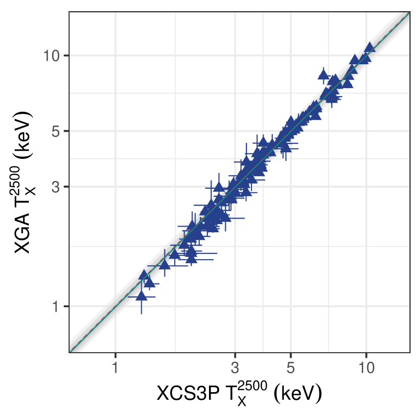
(a)	(b)

Figure 9: The Xga APEC temperatures versus the XCS3P APEC temperatures within $R_{500}$ (a) and $R_{2500}$ (b) for the SDSSRM-XCS sample (as taken from Giles et al., 2022). The red dashed line represents the 1:1 relation (note however, the dashed line may be hidden as the best-fit line is overplotted).

XXL-100-GC: The Xga analysis yielded T${}_{\rm X}^{\rm 300kpc}$ values for 97 of the 99 clusters in the input sample. The temperature comparison is shown in Figure 10. The best-fit normalisation of 0.99$\pm$0.01 shows that the Xga and Giles et al. (2016) values are in excellent agreement, despite the large number of differences between the two approaches (see Section 3.1.2).

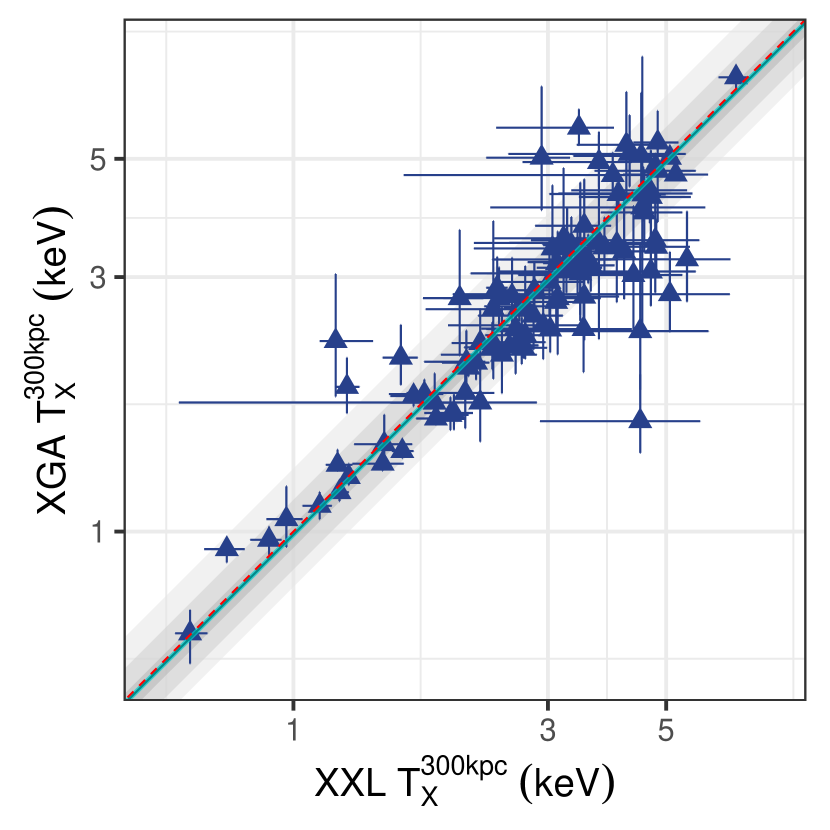
Figure 10: A comparison of global X-ray temperature values measured by Xga and XXL analyses (as taken from Giles et al., 2016), for the XXL-100-GC sample (see Section 3.2.1 for details). The 1:1 relation is highlighted by the red dashed line.

LoCuSS High-$\boldsymbol{L_{\rm{X}}}$: The Xga analysis yielded global, core-excised, temperatures values for all 32 of the input sample with XMM results in Mulroy et al. (2019). The temperature comparison is shown in Figure 11. The best-fit normalisation is 1.01$\pm$0.01, showing that the Xga and Mulroy et al. (2019) values are in excellent agreement, despite the large number of differences between the two approaches (see Section 3.1.3).

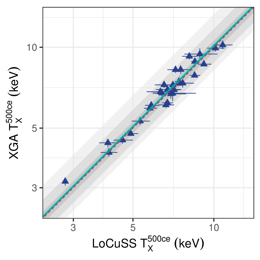
Figure 11: A comparison of global, core-excised, X-ray $R_{500}$ temperatures measured by Xga and LoCuSS analyses, for a subset of the LoCuSS High-$L_{\rm{X}}$ sample. The temperatures are measured within core excluded weak-lensing $R_{500}$ values (within [0.15-1]$R_{500}$), presented in Mulroy et al. (2019).

3.2.2 Validation of Xga derived $M_{\rm gas}$ values

XXL-100-GC: The Xga analysis yielded M${}_{\rm gas}^{500}$ values for 91 (of the 99) clusters contained in the XXL-100-GC sample. Figure 12 shows the comparison between Xga measured and gas mass estimates published in Eckert et al. (2016). While the best-fit normalisation of 0.89$\pm$0.06 highlights the Xga values are $\sim$10% lower than those measured by Eckert et al. (2016), the difference is $<$2$\sigma$. Therefore, there is broad agreement between the two analyses. This is encouraging considering the significant differences in density measurement between the two samples (see Section 3.1.2).

LoCuSS High-$\boldsymbol{L_{\rm{X}}}$: The Xga analysis yielded M${}_{\rm gas}^{500}$ values for 32 (of 33) LoCuSS High-$L_{\rm{X}}$ clusters. Note that the one cluster missing (RXCJ1212) Comparisons of the gas masses calculated within R₂₅₀₀ ($M_{\rm gas}^{2500}$) and R₅₀₀ ($M_{\rm gas}^{500}$) are presented in Figure 13 (a) and (b) respectively. The normalisations of the fits are 0.97$\pm$0.02 and 0.93$\pm$0.02 for $M_{\rm gas}^{2500}$ and $M_{\rm gas}^{500}$ respectively. This highlights that the $M_{\rm gas}^{2500}$ values are consistent, however, the XGA measured $M_{\rm gas}^{500}$ values are on average 7% lower than the LoCuSS values (significant at the 3.5$\sigma$ level).

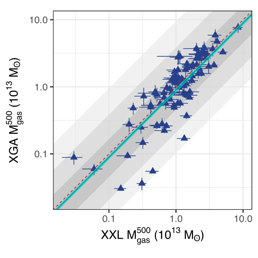
Figure 12: A one-to-one comparison of gas masses measured for the XXL-100-GC cluster sample, within $R_{500}$, by Eckert et al. (2016) and an Xga reanalysis. $S_{B}$ profiles were fitted with Beta models, density profiles with King models. Contains measurements for 91 of 96 XXL-100-GC clusters analysed with Xga.

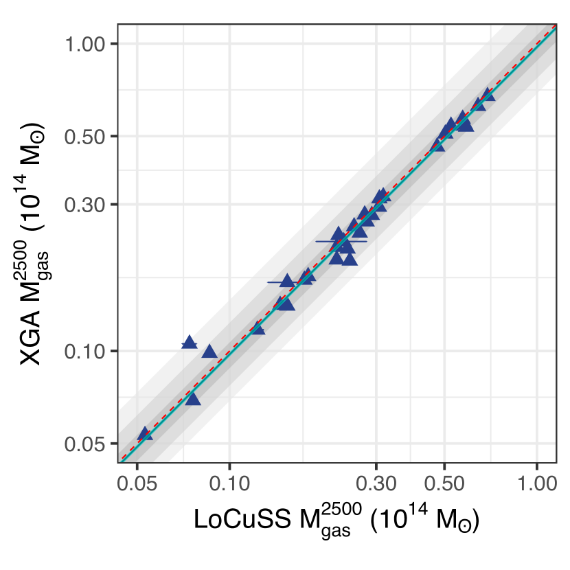
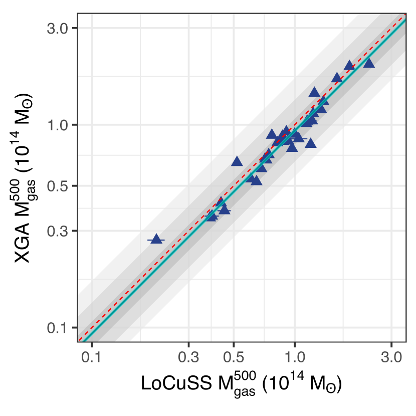
(a)	(b)

Figure 13: A one-to-one comparison of gas masses measured for the LoCuSS High-$L_{\rm{X}}$ cluster sample, within LoCuSS measured $R_{2500}$ (a) and $R_{500}$ (b) values, by Martino et al. (2014) and an Xga reanalysis.

3.2.3 Validation of Xga derived $M_{\rm hydro}$ values

LoCuSS High-$\boldsymbol{L_{\rm{X}}}$: Figure 14 shows a comparison between the Xga and LoCuSS hydrostatic masses for $M_{\rm{hy}}^{2500}$ (a) and $M_{\rm{hy}}^{500}$ (b). We successfully measure masses for 29 galaxy clusters (of 33) in the LoCuSS High-$L_{\rm{X}}$ sample, 24 of which have XMM hydrostatic masses measured by LoCuSS (which are compared in Fig. 14). When compared to the LoCuSS masses (specifically those measured by XMM), we find Xga measured masses 10% and 19% higher than LoCuSS for $M_{\rm{hy}}^{2500}$ and $M_{\rm{hy}}^{500}$ respectively. While the difference is significant at the 3.3$\sigma$ level for $M_{\rm{hy}}^{2500}$, the difference is $<$3$\sigma$ for $M_{\rm{hy}}^{500}$.

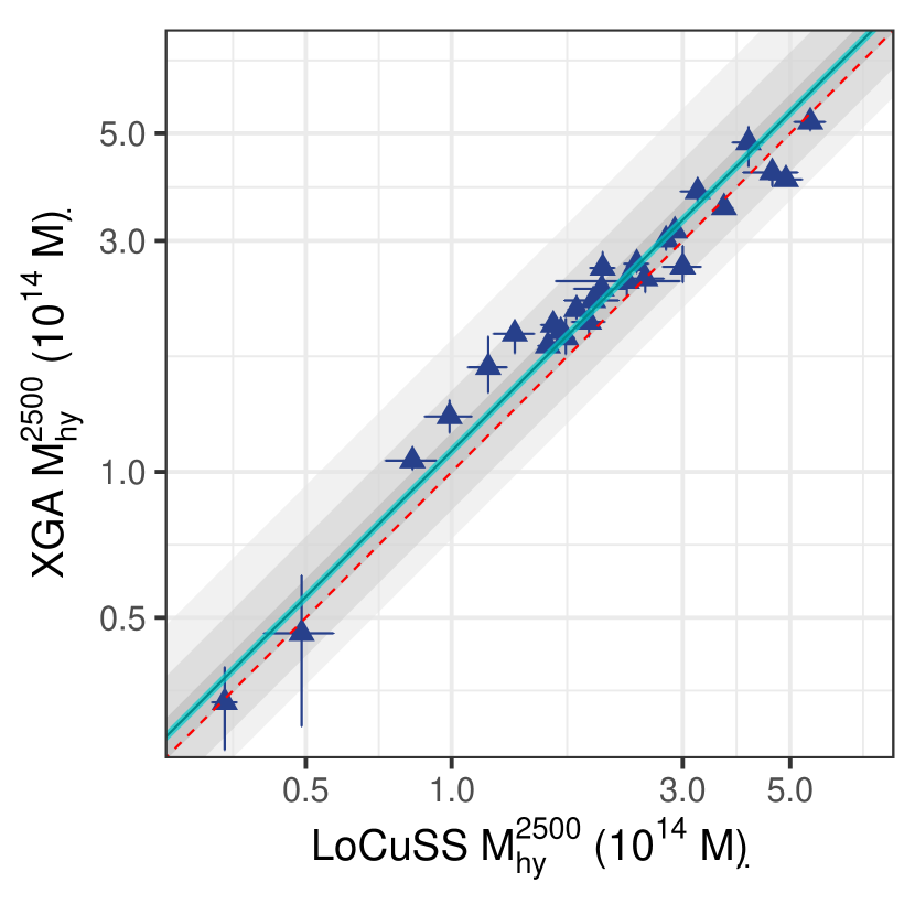
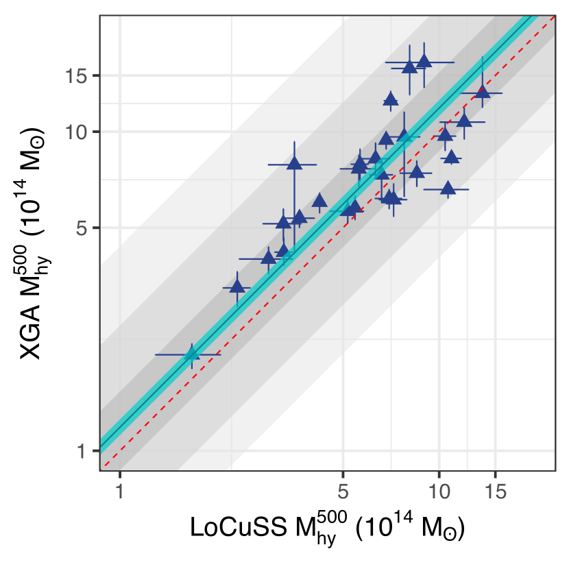
(a)	(b)

Figure 14: A one-to-one comparison of hydrostatic masses measured for the LoCuSS High-$L_{\rm{X}}$ cluster sample, within LoCuSS measured $R_{2500}$ (a) and $R_{500}$ (b) values, by Martino et al. (2014) and an Xga reanalysis.

3.3 Discussion

From the tests presented above, we can conclude that the Xga (almost) automated batch approaches to extracting estimates of $T_{\rm X}$, $M_{\rm gas}$ and $M_{\rm hydro}$ are robust (see Figures 9-14 and Table 3). In only 2 (out of 9) of the tests was the normalisation more than $3\sigma$ from unity. We have also effectively demonstrated the flexibility of our tools by matching as closely as possible the original analysis methodologies of three different samples; our use of the LoCuSS High-$L_{\rm{X}}$ and XXL-100-GC samples in particular also show that Xga can adapt to high and low signal-to-noise observations. All this illustrates that Xga can be used to easily derive properties for large sets of galaxy clusters. Uniquely, we have made Xga open and available for entire community to use, and we also make every effort to encourage its use by supplying extensive documentation and examples.

Where there are offsets, these are likely explained by the differing approaches taken during the analyses. In future work, we will further optimise the Xga method using mock observations of clusters extracted from hydrodynamic simulations (such as e.g., Cui et al., 2018; Pakmor et al., 2022), i.e. where the “true” gas and halo masses are known. This will also allow us to estimate the systematic errors introduced from simplifying assumptions, such as spherical symmetry and hydrostatic equilibrium. We also note that we have derived temperature profiles for all galaxy clusters for which a hydrostatic mass has been measured, whereas some previous work (e.g. Martino et al., 2014) assumes a temperature profile in cases where there are low total counts. As we apply Xga to the measurement of hydrostatic masses in the future we will work to implement improvements to our method, including modelling of the X-ray background to better support the analysis of low-redshift systems, and more sophisticated approaches to the deprojection of temperature profiles.

4 Mass analysis of the SDSSRM-XCS sample

Here we present hydrostatic masses for a subset of galaxy clusters in the SDSSRM-XCS sample presented by Giles et al. (2022).

4.1 Masses for a subset of the SDSSRM-XCS sample

We attempt to measure masses for all 150 galaxy clusters in the SDSSRM-XCS sample. Measurements presented in this section are performed using Xga, within the $R_{500}$ and $R_{2500}$ values measured by G22. In Section 3.2.1 we demonstrated that the global Xga $T_{\rm{X}}$ measurements are consistent with the original G22 analysis when measured within identical apertures (see Fig. 9).

Temperature and density profiles were generated out to $R_{500}$ (from G22), with the hydrostatic masses estimated from these profiles at $R_{500}$ and $R_{2500}$. Density profiles were generated as described in Section 2.8, and temperature profiles were generated and selected as described in Section 2.10 from annular spectra (described in Section 2.5).

We are able to successfully measure hydrostatic masses for 104 of the 150 galaxy clusters in the SDSSRM-XCS sample. The temperature profiles used for these measurements have between 4 (the minimum number allowed, see Section 2.5) and 26 annuli. This set of hydrostatic masses adds significant value to the SDSSRM-XCS sample, as well as representing one of the largest samples of cluster hydrostatic masses available. As each mass is measured individually, rather than derived through the stacking of different clusters (as is usually the case for weak lensing cluster masses), there are many possible uses for the sample. Also, as SDSSRM-XCS clusters were selected from optical/NIR via the SDSS redMaPPer catalogue (Rykoff et al., 2014), this sample allows for powerful multi-wavelength studies of how cluster mass is related to optical properties.

4.2 Comparison of SDSSRM-XCS masses with the literature

Here we compare the masses estimated for the SDSSRM-XCS sample in Section 4.1 to values taken from the literature. We compare the M${}^{500}_{\rm hy}$ values to those given in Martino et al. (2014), Lovisari et al. (2020) and Poon et al. (2023). The Martino et al. (2014) masses are from the LoCuSS sample as discussed in Section 3.1. The Lovisari et al. (2020) sample contains 120 XMM derived hydrostatic masses from Planck detected clusters (spanning a redshift range of $0.059<z<0.546$). Finally, Poon et al. (2023) estimate hydrostatic masses using XMM for 19 clusters contained in the Meta-Catalog of X-Ray Detected Clusters of Galaxies (Piffaretti et al., 2011) within the Hyper Suprime-Cam Subaru Strategic Programme field (Aihara et al., 2018). The 104 SDSSRM-XCS clusters with M${}^{500}_{\rm hy}$ values are matched to the samples of clusters used in the works listed, resulting in 21, 16 and 9 clusters matched to Martino et al. (2014), Lovisari et al. (2020) and Poon et al. (2023) respectively. The comparison of the masses is plotted in Figure 15(a). The black line represents the 1:1 relation, highlighting a broad consistency of the masses measured in this work and those reported in the literature.

In Figure 15(b), we show the number of SDSSRM-XCS clusters per M${}^{500}_{\rm hy}$ bin (given by the blue histogram). The M${}^{500}_{\rm hy}$ distributions from Martino et al. (2014) and Lovisari et al. (2020) are given by the brown and green spline curves respectively. While the SDSSRM-XCS sample clearly contains more masses than the Martino et al. (2014) sample, clusters in Martino et al. (2014) are selected by imposing a luminosity limit on clusters detected in the RASS, reducing the number of available clusters for study. The Lovisari et al. (2020) sample contains a larger number of masses overall, the SDSSRM-XCS sample provides many more low-mass cluster estimates. However, we note that this is due to the Planck selection of the clusters in Lovisari et al. (2020), which will select higher mass clusters. Additionally, Lovisari et al. (2020) provide masses for 17 clusters for which their masses were estimated using $<$4 temperature profile bins. For the analysis of the SDSSXCS-RM sample, we required a minimum of 4 bins in the temperature profile for a mass determination.

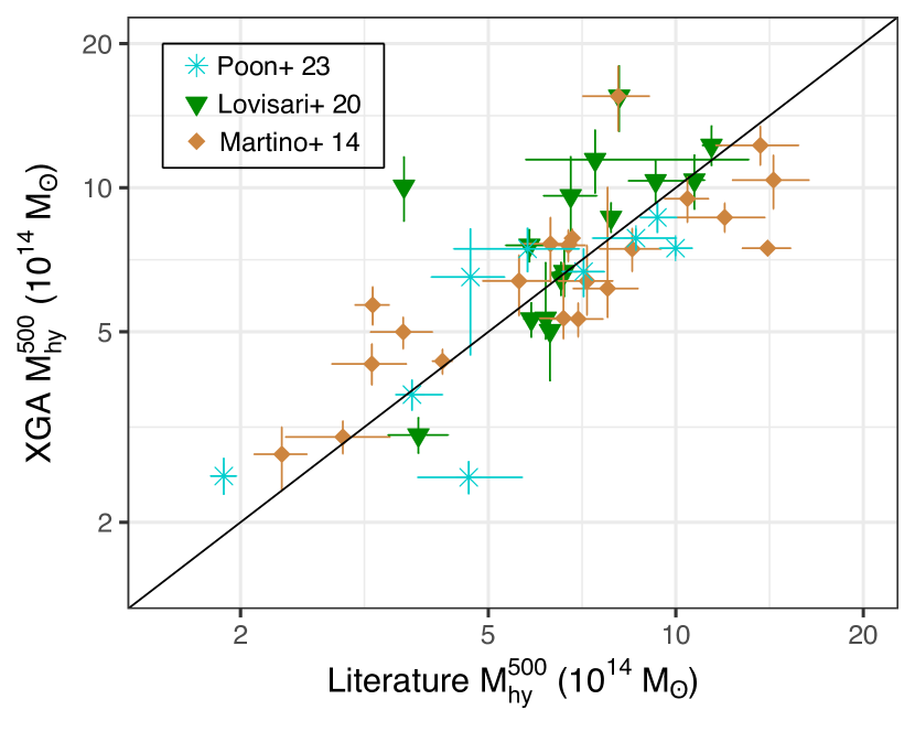
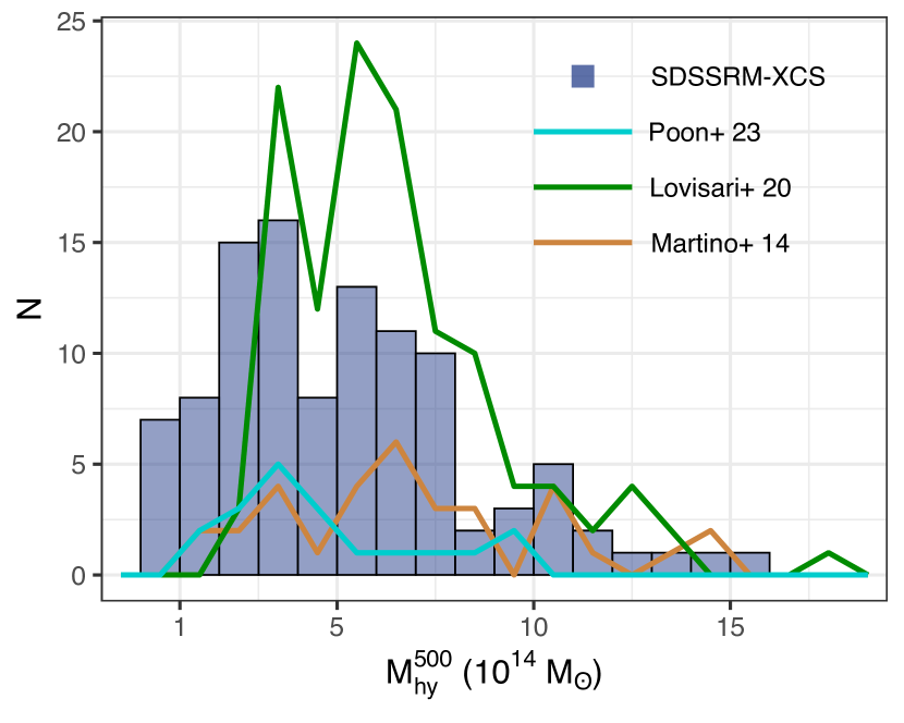
(a)	(b)

Figure 15: (a) A one-to-one comparison of hydrostatic masses measured for the SDSSRM-XCS cluster sample using Xga, compared to Martino et al. (2014, brown diamonds), Lovisari et al. (2020, green triangles) and Poon et al. (2023, cyan crosses). (b) Mass distribution of the 102 SDSSRM-XCS clusters with M${}^{500}_{\rm hy}$ values (lightblue histogram). Mass distributions from Martino et al. (2014, brown histogram, using only the XMM based masses), Lovisari et al. (2020, green) and Poon et al. (2023, cyan) are given for comparison.

5 Summary and next steps

Finally, in this section we present summaries of the work in this paper, discussions of the implications and results, and goals for related future work.

5.1 Summary

This work introduces an automated method, and tool (Xga), for measuring hydrostatic masses (and many other X-ray properties) of large samples of galaxy clusters. We summarise this tool, and the approaches taken to measure the various properties that are required to determine hydrostatic masses, in the first part of the paper. Two demonstration clusters (SDSSXCS-55 and SDSSXCS-6955) are used to help illustrate the different steps and data products required. This includes the measurement of density and 3D temperature profiles. As part of this we showcase and explain Xga’s PSF correction feature, which takes into account the spatially varying nature of XMM PSFs, and is relevant to the measurement of density profiles.

We then make use of three samples of galaxy clusters, SDSSRM-XCS, XXL-100-GC, and LoCuSS High-$L_{\rm{X}}$ to explore the efficacy of measurements of galaxy cluster properties produced by our new software tool, Xga. Once we have demonstrated that Xga is reliable, we find and present new measurements of hydrostatic mass for the SDSSRM-XCS sample. In summary:

• Comparisons of $T_{\rm{X}}$ measurements of the SDSSRM-XCS sample from an existing XCS analysis (Giles et al., 2022) to those measured by Xga demonstrate close agreement. This holds true for measurements within both $R_{500}$ and $R_{2500}$, with $R_{2500}$ measurements appearing to show less scatter. Close agreement of these measurements is expected because they use the same event lists and region files, as well as very similar analysis techniques. We quantify the comparisons by plotting Xga results against literature value and fitting a fixed-slope power law; all normalisations are consistent with unity.

• Similar comparisons of $T_{\rm{X}}$ to literature values measured for the XXL-100-GC (Giles et al., 2016) and LoCuSS High-$L_{\rm{X}}$ (Mulroy et al., 2019) samples showed good agreement, and also demonstrated Xga’s ability to perform measurements with different energy limits, with metallicity left free to vary, and different cosmologies. Model fits again showed that the comparison normalisations are consistent with unity.

• We then began to test values derived from radial profiles, starting with gas masses. Comparisons of gas mass values measured for the XXL-100-GC (Eckert et al., 2016) and LoCuSS High-$L_{\rm{X}}$ (Martino et al., 2014) samples, and reanalyses using Xga, demonstrated that Xga produces gas mass measurements consistent with past work. The XXL comparison indicated an small ($\sim$10%) offset between the two analysis, however, the difference was not significant. The LoCuSS comparison demonstrated a 1:1 relation between gas masses measured within LoCuSS $R_{2500}$ values, but that $R_{500}$ gas masses are slightly systematically larger when measured by Xga versus the original work.

• Our final comparison makes use of the hydrostatic masses measured within $R_{2500}$ and $R_{500}$ for the LoCuSS High-$L_{\rm{X}}$ sample by Martino et al. (2014). The $M^{\rm{hy}}_{2500}$ comparison lies close to the 1:1 line, with minimal scatter. The $M^{\rm{hy}}_{500}$ comparison is also broadly compatible with the 1:1 line, though the scatter and uncertainties are increased when compared to the $M^{\rm{hy}}_{2500}$ plot. From this comparison, and the others presented in this work, we conclude that Xga mass measurements are consistent with previous work and can be relied on.

• Finally, we present new measurements of hydrostatic mass for the SDSSRM-XCS galaxy cluster sample. In total, we measure hydrostatic masses for 104 (out of 150) clusters, which is comparable to the largest consistently analysed and measured X-ray based hydrostatic masses in the literature.

• We have demonstrated that Xga is a mature tool that is capable of measuring many key properties of galaxy clusters, and easily replicating existing analyses, producing comparable results. Any Xga analysis is easy to scale to any size of sample. It also allows colleagues without specialist X-ray experience to carry out their own cluster mass analyses.

5.2 Future Work

Here we detail some of the work that we have planned for our new implementation of hydrostatic mass measurement, as well as for the samples of masses we have (and will) measure.

5.2.1 Mass-Observable Relations

Whilst we have demonstrated the utility of Xga for measuring hydrostatic masses for large samples of galaxy clusters, and measured masses for a significant number of clusters using archival data, we have not yet constructed mass-observable relations. As we discussed in the introduction, such relations are an invaluable independent measure of the normalisation, slope, and scatter of cluster masses with other observables. The next paper in this series will focus on constructing such relations for a larger set of galaxy clusters, and for both X-ray and optically derived observables; they will be extremely useful for the next-generation of cluster cosmology being enabled by new telescopes and missions.

5.2.2 Other Samples

We will produce mass measurements and scaling relations for other samples of galaxy clusters, selected from optical/NIR surveys such as DES, and from the ACT-DR5 cluster catalogue. This shall not only add a significant number of cluster masses to our sample, but will also open the possibility of constructing scaling relations between X-ray mass and Sunyaev–Zeldovich properties.

5.2.3 Temperature Profile Methodology

In this initial work we have used a relatively simple methodology to ‘deproject’ the measured temperature profiles and infer the three-dimensional radial temperature structure of the galaxy clusters. More sophisticated techniques could be applied to this problem (such as deep learning deprojection, Iqbal et al., 2023), which might improve the temperature profiles measured by Xga, and thus the hydrostatic masses. This will be achievable through the existing framework of Xga, and future work with different techniques to measure 3D temperature profiles would also provide a systematic comparison between the measured profiles, and inferred masses.

We will also improve the sophistication of the spectral fits used to generate the projected temperature profiles, taking more care to account for the effects of the XMM PSF on the photons detected within each annulus.

5.2.4 Multi-mission X-ray Analyses

Planned additions to the Xga software package will enable support for X-ray telescopes other than XMM; e.g. Chandra, eROSITA, and XRISM. This will allow a user to draw on multiple archives of X-ray observations for analysis of samples, increasing the likelihood that samples selected from other wavelengths will have a serendipitous X-ray observation.

Multi-mission support will also allow us to design joint analyses that take advantage of the unique capabilities of each telescope. Joint analyses with all available X-ray data should be- come routine, rather than requiring special effort, and Xga can provide that capability.

We will also include support for simulated telescopes to enable preparatory work for future missions; e.g. Athena, Lynx, and AXIS. As such we will produce catalogues of hydrostatic masses measured with multiple current telescopes (XMM and Chandra), as well as explore how we may exploit the capabilities of planned telescopes. Work on simulated clusters will also include exploration of the hydrostatic mass bias from true mass.

5.2.5 Accounting for non-thermal pressure support

Hydrostatic masses are biased from true masses due to assumptions made during the derivation of Equation 1. The assumption of hydrostatic equilibrium implies that all pressure support is provided by the thermal gradient of the ICM, which is not the case. Various processes also help to balance gravitational collapse, and together are often referred to as non-thermal pressure (NTP) support. Methods to measure a total mass from X-ray observations exist (e.g. Eckert et al., 2019), and we aim to apply them to large samples of clusters such as SDSSRM-XCS. By taking NTP support into account hydrostatic masses can become even more competitive with other direct mass measurement methods (such as individual weak lensing).

Data Availability

The XMM data underlying this article were accessed from the XMM science archive. The derived data underlying this article are available in the article and in its online supplementary material. All analysis code is available in the accompanying GitHub repositories.

Appendix A Fitting models to radial profiles in Xga

Table 4: Summaries of the Xga 1D radial models used in this work (though others are implemented and available). Model names and descriptions of their use are included. The units of model parameters are given, as well as the start parameters used for initial fits. Finally details of the parameter priors used for the full MCMC fit are given, where $\mathcal{U}$[A, B] indicates a uniform distribution with limits A and B.

Model Name	Equation	Brief description	Parameters	Start Values	Priors
Beta	$S_{X}(R)=S_{0}\left(1+\left(\dfrac{R}{R_{c}}\right)^{2}\right)^{-3\beta+0.5}$	Simple model for the	$S_{0}$ [$\rm{ct}\rm{s^{-1}}\>\rm{arcmin}^{-2}$]	1	$\mathcal{U}$[0, 3]
		surface brightness profile,	$R_{\rm{core}}$ [kpc]	100	$\mathcal{U}$[1, 2000]	11
		Cavaliere & Fusco-Femiano (1976).	$\beta$	1	$\mathcal{U}$[0, 3]
King	$\rho_{g}(R)=\rho_{0}\left(1+\left(\dfrac{R}{R_{c}}\right)^{2}\right)^{-3\beta}$	A very simple model for the	$\rho_{0}$ [$\rm{M_{\odot}}\rm{Mpc^{-3}}$]	1	$\mathcal{U}$[1, 10000]$\times 10^{12}$
		density profile; an inverse-Abel	$R_{\rm{core}}$ [kpc]	100	$\mathcal{U}$[0, 2000]	12
		transform of the beta profile.	$\beta$	1	$\mathcal{U}$[0, 3]
Simplified Vikhlinin Temperature	$T(R)=\dfrac{T_{0}\left(\left(\frac{R}{R_{c}}\right)+\frac{T_{min}}{T_{0}}\right)\left(\frac{R^{2}}{R_{T}^{2}}+1\right)^{-\frac{c}{2}}}{\left(\frac{R}{R_{c}}\right)^{a_{c}}+1}$		$R_{\rm{c}}$ [kpc]	50	$\mathcal{U}$[10, 500]
		Simplified Vikhlinin et al. (2006)	$a_{\rm{c}}$	1	$\mathcal{U}$[0, 5]
		temperature profile as used by	$T_{\rm{min}}$ [keV]	3	$\mathcal{U}$[0.1, 6]	13
		Ghirardini et al. (2019).	$T_{0}$ [keV]	6	$\mathcal{U}$[0.5, 15]
			$R_{\rm{T}}$ [kpc]	200	$\mathcal{U}$[100, 500]
			c	1	$\mathcal{U}$[0, 5]

Various aspects of this work require models to be fitted to radial data profiles. For this work we make use of the emcee ensemble MCMC sampler which has been widely used in the astronomy community (Foreman-Mackey et al., 2013). This sampler runs multiple interconnected MCMC chains to explore the parameter space. We choose to use a simple Gaussian likelihood function and uninformative uniform priors. The priors are dependant upon the particular profile being fitted, as well as the model choice, and further information can be found in table 4.

All profile fitting performed for this work used an emcee sampler instance with 20 walkers, each taking 30000 steps. We chose to generate sets of start positions for the walkers by adapting a simple method suggested in the emcee documentation. We use the SciPy (Virtanen et al., 2020) implementation of the non-linear least squares (NLLS) fitting method (curve_fit) to fit the model to the profile. The NLLS fits use starting values for model parameters as defined in Table 4. We then find the order of magnitude of each fit parameter. These are then perturbed by drawing an $N_{\rm{walker}}\times N_{\rm{par}}$ matrix of random values from a $\mathcal{N}(0,1)$ distribution, multiplying each random value by the order of magnitude of the respective parameter, and then adding this perturbation to the original NLLS best fit value. Before starting, the sampler checks to ensure that the start positions all fall within the allowed boundaries of the priors, and if not then they are re-drawn until they do.

Once the sampler run is complete, we calculate integrated autocorrelation times for the model parameters, if all autocorrelation times are more than 400 times smaller than the number of steps taken by a walker, then we find the mean autocorrelation time for all the parameters, round it up to the nearest 100, and double it to find a good number of steps to remove from each walker’s chains as a burn-in period. If any of the parameters had an autocorrelation time that did not fit this criteria, then we take a brute force approach and remove the first 30% of steps in each walker’s chains. We draw 10000 random points from combined parameter chains from all walkers to create the final posterior distributions. We also measure medians of the parameter posterior distributions, as well as finding the 1$\sigma$ regions.

These fits are performed using a set of radial model classes that we have implemented in Xga. They provide easy access to model posterior distributions, visualisations, and predictions. Xga models also have implementations of useful mathematical operations such as differentiation, spherical volume integration, and inverse Abel transformation of the models (using PyAbel; Hickstein et al., 2019; Gibson et al., 2022), making use of Astropy (Astropy Collaboration et al., 2013, 2018) to provide correct units for any calculated quantities. Model instances also provide information on model parameters, support custom start parameters, and also custom priors.

Appendix B Companion GitHub Repository

The work in this paper is accompanied by a GitHub repository${}^{\ref{foot:gitrepo}}$, containing the samples and code required to reproduce our work, as well as tables of results and extra figures. Here we briefly summarise the contents of the repository and provide the context which connects sections of the paper to the different files. The vast majority of files containing sample information and results are ‘comma separated variable’ files (csv), which are human-readable and can be opened in a text editor, or more practically can be opened with software such as TOPCAT (Taylor, 2005), or a Python module such as Pandas (Wes McKinney, 2010). Our companion repository contains several directories:

B.1 Sample Files

This part of the repository contains files of galaxy cluster properties for the samples used in this work. The exact contents of the sample files varies, but at minimum they contain a cluster name, a central coordinate, a redshift measurement, and some measurements of X-ray cluster properties that are used as validation at some point in this work;

• xcs3p_sdssrm_clusters.csv - A sample file containing the properties measured for the volume complete, temperature within $R_{500}$ fractional uncertainty less than 25%, SDSSRM-XCS sample of clusters presented by Giles et al. (2022). This sample is introduced in Section 3.1.1, and is used both for validation purposes, and for the measurement of new hydrostatic masses. The file includes X-ray centroid positions, redshifts, $R_{500}$ and $R_{2500}$ values (with uncertainties), $T_{\rm{X}}$, and $L_{\rm{X}}$ values within the two apertures. Not all clusters in this sample have $R_{2500}$ values and associated $L_{\rm{X}}$ and $T_{\rm{X}}$ values measured within them.

• xxl_gc100.csv - A file with information relevant to the XXL-100-GC sample of galaxy clusters, introduced in Section 3.1.2. The information available includes positions, redshifts, and $R_{500}$ measurements for the clusters, as well as XXL names and quality flags. Derived properties such as $T_{\rm{X}}$ and $L_{\rm{X}}$, measured by Giles et al. (2016), and gas mass values measured by Eckert et al. (2016), are also included. All data, apart from $R_{500}$ uncertainties, are taken from the XXL-100-GC VizieR table; the radius uncertainties are extracted from Eckert et al. (2016).

• locuss_highlx_clusters.csv - This contains information and properties for the clusters in the LoCuSS High-$L_{\rm{X}}$ sample, introduced in Section 3.1.3. A combination of overdensity radii, gas masses, and hydrostatic masses presented by Martino et al. (2014), as well as positions, redshifts, $T_{\rm{X}}$, and $L_{\rm{X}}$ measurements acquired via private communications.

We also provide a notebook that summarises the clusters in the samples; see Appendix B.3. This notebook generates the final file in the this part of the companion repository, combined_sample_duplicates.csv, that details which of the clusters in each sample appear in another of the validation samples. This information is used in Section 3.1 to state the number of unique clusters in our combined validation samples.

B.2 Data Notes

A small, but important, part of this paper’s companion repository, that includes notes made on the data used during analysis of the clusters in this work. This is relevant to all results presented in this paper. We include the following files:

• flare_check_notes.md - We performed manual inspections of all the observations that Xga selected for the three samples used in this work, to check for evidence of residual flaring that could affect our results. This file contains the observation identifiers of the data that we decided to exclude, and in some cases provides extra context as to the reason.

• obs_blacklist.csv - This file contains the exact data we excluded from use, in a form that Xga recognises and can use as a ‘blacklist’.

• obs_info.json - Here we detail which XMM observations are used in the analysis of which galaxy clusters. The file is human readable, and can be used to deduce which data are relevant to which clusters, but can also be read as a Python dictionary. The top-level keys are XMM ObsIDs, and each is accompanied by a list of cluster names.

B.3 Notebooks

• sample_properties.ipynb - This includes the information available in each dataset, the positions of the clusters on the sky, and whether there any common clusters between the samples.

• demonstration_clusters.ipynb - Here we select our two example clusters, SDSSXCS-55 and SDSSXCS-6955, and generate every figure included in Section 2. The information in Table 1 is also shown here.

• common.py - This contains variable definitions that are common to multiple notebooks, so any change is reflected in the entire analysis once re-run. This includes the cosmology definitions and colour selections for our three validation samples. We also include comparison and plotting functions common to multiple notebooks, these are used to generate the one-to-one comparison figures in Section 3.

• visualisations_region_adjustment - This is a directory, containing several notebooks related to the visualisation of our clusters, and the modification of the relevant region files.

  • visualise_analysis_regions.ipynb - In this notebook we create visualisations of the XMM observations of the clusters in the three samples. We also overlay region information, and save the images as an output (see Appendix B.4).

  • *_region_checks.ipynb - This represents three notebooks (with the ‘*’ replaced by ‘sdssrm-xcs’, ‘xxl’, and ‘locuss’) that serve the same purpose for each of our three samples introduced in Section 3.1. Here we used the Xga region editor (see Table 10) to make manual adjustments to the regions used to remove contaminating sources from the analyses of each sample. These notebooks are relevant to Section 2.4.

• temp_lum_comparisons - We store notebooks relevant to the measurement of X-ray temperatures and luminosities for our three samples. These measurements are used for comparisons of Xga measurements to literature values, as seen in Section 3.2.1.

  • sdss_comparisons.ipynb - Xga measurements of temperature and luminosity, within both $R_{500}$ and $R_{2500}$ (where available), are performed here for the SDSSRM-XCS sample (Section 3.1.1).This notebook is used to create Figure 9. We also measure ‘core-excised’ properties for SDSSRM-XCS.

  • xxl_comparisons.ipynb - Xga measurements of temperature and luminosity within a 300 kpc aperture for the XXL sample (Section 3.1.2) are made in this notebook. We also create Figure 10 by comparing to the original XXL temperature measurements (Giles et al., 2016).

  • locuss_comparisons.ipynb - This notebook contains Xga measurements of temperature and luminosity for the LoCuSS High-$L_{\rm{X}}$ sample (Section 3.1.3). The comparisons made to literature values are shown in Figure 11.

• gas_mass_comparisons - A directory containing notebooks relevant to the comparison of literature gas mass measurements to Xga measurements, as seen in Section 3.2.2.

  • xxl_gm_comparisons.ipynb - Xga measurements of gas mass for the XXL-100-GC sample within published $R_{500}$ (with radius error propagated) are performed here. Comparisons, as discussed in Section 3.2.2, are performed, and the notebook is used to generate Figure 12.

  • locuss_gm_comparisons.ipynb - Xga measurements of gas mass for the LoCuSS High-$L_{\rm{X}}$ sample within published $R_{5}00$ and $R_{2500}$ values are performed here. Comparisons, as discussed in Section 3.2.2, are performed, and the notebook is used to generate Figure 13.

• hydro_masses Finally, this directory contains notebooks relevant to the measurement of hydrostatic masses for two of the cluster samples used in this work.

  • locuss_hym_comparisons.ipynb - Xga measurements of hydrostatic mass for LoCuSS High-$L_{\rm{X}}$ galaxy clusters are performed here, within both $R_{500}$ and $R_{2500}$ radii. In Section 3.2.3 they are compared to the literature values measured using XMM. This notebook is used to generate Figure 14.

  • sdssrm-xcs_new_masses.ipynb - In this notebook we measure new hydrostatic masses for the SDSSRM-XCS sample of galaxy clusters, as presented in Section 4.

B.4 Outputs

In this final part of the companion repository, we store the main outputs of this work.

• cluster_visualisations - This directory contains combined XMM images of the clusters in the three samples, with one sub-directory for each sample. The file name used for each image is the name of the galaxy cluster used in this work, a mask has been applied, and contaminating source regions are overlaid.

• custom_regions - This contains region files which were modified during the course of Section 2.4. They are in sky (RA-Dec) coordinates, and in the FK5 coordinate frame.

• figures - Figures created for this paper are stored in this directory.

• results - All sets of results measured during the course of this work are stored in here, including Xga measured properties for the SDSSRM-XCS, XXL-100-GC, and LoCuSS High-$L_{\rm{X}}$ samples. Tables 5, 6, 7, and 8 contain a subset of the results, and define the columns.

Appendix C Tables of properties

C.1 SDSSRM-XCS Xga properties

Table 5: Properties of the SDSSRM-XCS galaxy cluster sample. All uncertainties calculated from 68% confidence limits, equivalent to $1\sigma$. For brevity, the first entry of the Table is given, with the full Table available from https://github.com/DavidT3/XCS-Mass-Paper-I-Analysis/tree/master/outputs/results.
(1) redMaPPer ID of the cluster; (2) Right ascension as defined by redMaPPer; (3) Declination taken from redMaPPer; (4) redshift taken from redMaPPer; (5) $R_{500}$ taken from Giles et al. (2022); (6) $R_{2500}$ taken from Giles et al. (2022); (7) X-ray Temperature determined within $R_{2500}$; (8) X-ray temperature determined within $R_{500}$; (9) Gas mass determined within $R_{2500}$; (10) Gas mass determined within $R_{500}$; (11) Mass determined from the hydrostatic mass analysis described throughout Section 2, within $R_{2500}$; (12) Mass determined from the hydrostatic mass analysis described throughout Section 2, within $R_{500}$.

(1)	(2)	(3)	(4)	(5)	(6)	(7)	(8)	(9)	(10)	(11)	(12)
RM ID	RA	Dec	z	$R_{500}$	$R_{2500}$	$T_{\rm{X}}^{2500}$	$T_{\rm{X}}^{500}$	$M^{\rm{gas}}_{2500}$	$M^{\rm{gas}}_{500}$	$M^{\rm{hy}}_{2500}$	$M^{\rm{hy}}_{500}$
	(deg)	(deg)		(kpc)	(kpc)	(keV)	(keV)	1014 (M⊙)	1014 (M⊙)	1014 (M⊙)	1014 (M⊙)
2	250.08	46.71	0.23	1503	644	9.73${}^{+0.20}_{-0.20}$	10.40${}^{+0.24}_{-0.22}$	0.59${}^{+0.00}_{-0.00}$	1.68${}^{+0.00}_{-0.00}$	4.48${}^{+0.26}_{-0.26}$	10.36${}^{+1.31}_{-1.34}$

C.2 XXL-100-GC Xga Reanalysis Results

Table 6: Properties of the XXL-100-GC galaxy cluster sample. All uncertainties calculated from 68% confidence limits, equivalent to $1\sigma$. For brevity, the first entry of the Table is given, with the full Table available from https://github.com/DavidT3/XCS-Mass-Paper-I-Analysis/tree/master/outputs/results.
(1) XLSSC ID as given in Pacaud et al. (2016); (2) Right ascension as given in Pacaud et al. (2016); (3) Declination as given in Pacaud et al. (2016); (4) redshift as given in Pacaud et al. (2016); (5) $R_{500}$ as given in Eckert et al. (2016); (6) Xga measured X-ray temperature within 300 kpc; (7) Xga measured gas mass within $R_{500}$.

(1)	(2)	(3)	(4)	(5)	(6)	(7)
XLSSC	RA	Dec	z	$R_{500}$	$T_{\rm{X}}^{\rm 300kpc}$	$M^{\rm{gas}}_{500}$
	(deg)	(deg)		(kpc)	(keV)	1014 (M⊙)
1	36.24	-3.82	0.614	777	3.41${}^{+0.47}_{-0.38}$	0.31${}^{+0.07}_{-0.07}$

C.3 LoCuSS High-$L_{\rm{X}}$ Xga Reanalysis Results

Table 7: LoCuSS High-$L_{\rm{X}}$ (a) galaxy cluster properties. All uncertainties calculated from 68% confidence limits, equivalent to $1\sigma$. For brevity, the first entry of the Table is given, with the full Table available from https://github.com/DavidT3/XCS-Mass-Paper-I-Analysis/tree/master/outputs/results.
(1) Cluster name; (2) Right ascension; (3) Declination; (4) redshift; (5) $R_{2500}$ overdensity radius; (6) $R_{500}$ overdensity radius; (7) Xga measured gas mass within $R_{2500}$; (8) Xga measured gas mass within $R_{500}$; (9) Xga measured hydrostatic mass within $R_{2500}$; (10) Xga measured hydrostatic mass within $R_{500}$. Values for columns (2) - (6) are taken from Martino et al. (2014).

(1)	(2)	(3)	(4)	(5)	(6)	(7)	(8)	(9)	(10)
Name	RA	Dec	z	$R_{2500}$	$R_{500}$	$M^{\rm{gas}}_{2500}$	$M^{\rm{gas}}_{500}$	$M^{\rm{hy}}_{2500}$	$M^{\rm{hy}}_{500}$
	(deg)	(deg)		(kpc)	(kpc)	1014 (M⊙)	1014 (M⊙)	1014 (M⊙)	1014 (M⊙)
Abell 0068	9.2785	9.1566	0.255	580	1400	0.32${}^{+0.00}_{-0.00}$	0.83${}^{+0.00}_{-0.00}$	3.79${}^{+0.18}_{-0.18}$	9.68${}^{+0.99}_{-0.97}$

Table 8: Properties of the LoCuSS High-$L_{\rm{X}}$ (b) galaxy cluster sample. All uncertainties calculated from 68% confidence limits, equivalent to $1\sigma$. For brevity, the first entry of the Table is given, with the full Table available from https://github.com/DavidT3/XCS-Mass-Paper-I-Analysis/tree/master/outputs/results.
(1) Cluster name; (2) Right ascension; (3) Declination; (4) redshift; (5) $R_{500}$ overdensity radius determined from a weak lensing analysis (see Okabe & Smith, 2016, values were provided by G. Smith via priv. comm.); (6) Xga measured core-excluded X-ray temperature within [0.15-1]$R_{\rm WL,500}$.

(1)	(2)	(3)	(4)	(5)	(6)
Name	RA	Dec	z	$R_{{\rm WL},500}$	$T_{\rm{X}}^{\rm 500ce}$
	(deg)	(deg)		(kpc)	(keV)
Abell 0068	9.2785	9.1566	0.255	1231	7.33${}^{+0.12}_{-0.12}$

Appendix D Relevant Xga commands and classes

Table 9: The Xga product classes used in this work (with a link to their API documentation), where they can be found in the hierarchy of Xga v0.4.2, a brief summary of their purpose and capabilities, and the most relevant section of this paper that they were used in.

Link to Xga Documentation	Xga Hierarchy	Summary	Section
Image	products.phot	Provides an Xga interface to FITS images, with easy access to the data and headers (read into memory only when needed), and convenient methods for coordinate conversion and creating visualisations.	§ 2.2
ExpMap	products.phot	Identical in function to Image, but provides an interface for exposure maps.	§ 2.2
RateMap	products.phot	Provides an interface to count-rate maps, constructed from Image and ExpMap instances. Has all Image functionality, as well as extra methods to calculate signal-to-noise within a specified region.	§ 2.2
Spectrum	products.spec	Provides an Xga interface to FITS spectra, with access to data and headers, as well as the ancillary files (background spectra, ARF, and RMF). Can store model fit information, and create visualisations of the spectra and effective area curve.	§ 2.5
AnnularSpectra	products.spec	Constructed from a set of Spectrum objects which have been generated in concentric annuli, this product provides similar access to data and model fits. Visualisation methods are also included, to view spectra from multiple annuli at once or view all spectra for the same annulus.	§ 2.5
ProjectedGasTemperature1D	products.profile	Contains projected temperature profile information (i.e. the temperatures measured by fitting the AnnularSpectra components with xspec). All Xga profiles have the ability to fit Xga models to their data, produce visualisations, and provide easy access to their data.	§ 2.5
APECNormalisation1D	products.profile	Similar to the ProjectedGasTemperature1D profile, but containing APEC normalisations from the fitting of an AnnularSpectra.	§ 2.5
EmissionMeasure1D	products.profile	An Xga profile class for emission measure. They can be produced from APECNormalisation1D profiles.	§ 2.5
GasDensity3D	products.profile	Xga profile class for the 3D hot gas density (either number or mass density). Can calculate a gas mass within a specified radius, assuming spherical symmetry.	§ 2.8
GasTemperature3D	products.profile	Xga profile class for deprojected (i.e. three-dimensional) hot gas temperatures.	§ 2.10
HydrostaticMass	products.profile	Represents a hydrostatic mass profile calculated from a GasTemperature3D and GasDensity3D profile. Contains extra methods to calculate a hydrostatic mass at a particular radius, as well as visualising the posterior distribution.	§ 2.11
BetaProfile1D	models.sb	Xga model class for the simplest model of a galaxy cluster X-ray surface brightness profile. These model classes can create basic visualisations of the current shape of the model, store parameter values and distributions, and perform mathematical tasks like differentiation, spherical integration, and Abel transforms.	§ 2.7
KingProfile1D	models.density	Xga model class for the simplest model of a galaxy cluster 3D density profile, deriving from the BetaProfile1D.	§ 2.8
SimpleVikhlininTemperature1D	models.temperature	Xga model class for a simplified version of the Vikhlinin model for the 3D temperature profile of the ICM.	§ 2.10

Table 10: Xga methods and functions used in this work (with a link to their API documentation), where they can be found in the hierarchy of Xga v0.4.2, a brief summary of their purpose and capabilities, and the most relevant section of this paper that they were used in. This is not an exhaustive list of every function called in the course o these analyses, but are the most salient to understanding what we did with Xga to achieve our results.

Link to Xga Documentation	Xga Hierarchy	Summary	Section
simple_xmm_match	sourcetools.match	Returns ObsIDs within a specified distance from the input $\alpha$ and $\delta$ values.	§ 2.1
edit_regions	products.phot.Image	Method of Image to show an interactive image to add and modify source regions.	§ 2.4
view	products.phot.Image	Make visualisations of Image, ExpMap, and RateMap, built into the classes. Can be configured to add overlays and masks.	§ 2.2
radial_brightness	imagetools.profile	Constructs radial surface brightness profiles from concentric circular annuli.	§ 2.7
fit	products.base. BaseProfile	A method of all Xga profile classes, which can fit models to their data and store the resulting information within the profile.	App. A
norm_conv_factor	sources.extended. GalaxyCluster	Calculates count-rate to APEC normalisation conversion factors for use on surface brightness profiles (both individual instrument and combined).	§ 2.8
shell_ann_vol_intersect	sourcetools.deproj	Calculates the volume intersection matrix of a set of circular annuli and a set of spherical shells	§ 2.10
single_temp_apec	xspec.fit.general	A function which fits emission models to spectra (either in a circular aperture or a single annulus) in order to measure ‘global properties’. Information on inner and outer radii is taken as an argument, to retrieve the correct spectra or generate them.	§ 2.5
single_temp_apec_profile	xspec.fit.profile	A function which fits emission models to a set of annular spectra (taking information about the fit configuration, as well as the size and number of the annuli so that it can generate them if they do not exist). This function specifically fits absorbed single-temperature APEC models.	§ 2.5
inv_abel_dens_onion_temp	sourcetools.mass	Calls other Xga functions (see the next two entries) to generate 3D density and temperature profiles, then combines them into hydrostatic mass profiles.	§ 2.11
onion_deproj_temp_prof	sourcetools.temperature	This function infers the 3D temperature profile from a projected temperature profile via the onion peeling method. If no projected temperature profiles exist they are generated by calling min_cnt_proj_temp_prof.	§ 2.10
min_cnt_proj_temp_prof	sourcetools.temperature	Uses a user-specified minimum number of counts and minimum annulus width to define annular regions and generate a projected temperature profile. This is achieved by calling single_temp_apec_profile, which will both ensure that the spectra have been generated, and fit them with emission models.	§ 2.10
inv_abel_fitted_model	sourcetools.density	Generates 3D gas density profiles by the surface-brightness profile method, converting them to 3D emissivity via an inverse abel transform, and from there to density by a count-rate to APEC normalisation factor.	§ 2.8

References

- Abbott et al. (2020) Abbott T. M. C., et al., 2020, Phys. Rev. D, 102, 023509
- Aihara et al. (2018) Aihara H., et al., 2018, PASJ, 70, S4
- Anders & Grevesse (1989) Anders E., Grevesse N., 1989, Geochimica Cosmochimica Acta, 53, 197
- Arnaud (1996) Arnaud K. A., 1996, in Jacoby G. H., Barnes J., eds, Astronomical Society of the Pacific Conference Series Vol. 101, Astronomical Data Analysis Software and Systems V. p. 17
- Astropy Collaboration et al. (2013) Astropy Collaboration et al., 2013, A&A, 558, A33
- Astropy Collaboration et al. (2018) Astropy Collaboration et al., 2018, AJ, 156, 123
- Bartalucci et al. (2017) Bartalucci I., et al., 2017, A&A, 608, A88
- Bartalucci et al. (2018) Bartalucci I., Arnaud M., Pratt G. W., Le Brun A. M. C., 2018, A&A, 617, A64
- Burke et al. (2022) Burke C. J., et al., 2022, MNRAS, 516, 2736
- Cash (1979) Cash W., 1979, ApJ, 228, 939
- Cavagnolo et al. (2009) Cavagnolo K. W., Donahue M., Voit G. M., Sun M., 2009, ApJS, 182, 12