Cosmic Ray Feedback on Bi-stable ISM Turbulence

Abstract

Despite being energetically important, the effect of cosmic rays on the dynamics of the interstellar medium (ISM) is assumed to be negligible because the cosmic ray energy diffusion coefficient parallel to the magnetic field is relatively large. Using numerical simulations, we explore how variation of the cosmic ray diffusion coefficient as a function of gas temperature could impact the dynamics of the ISM. We create a two-zone model of cosmic ray transport, reflecting the strong damping of the small scale magnetic field fluctuations, which scatter the cosmic rays, in a gas with low ionization. The variable diffusion coefficient allows more cold gas to form. However, setting the diffusion coefficient at a critical value in the warm phase allows the cosmic rays to adjust the kinetic energy cascade. Specifically, we show the slope of the cascade changes for motion perpendicular to the mean magnetic field, whereas kinetic energy parallel to the magnetic field is reduced equally across inertial scales. We show that cosmic ray energization (or reacceleration) comes at the expense of total radiated energy generated during the formation of a cold cloud. We also show that our two-zone model of cosmic ray transport is capable of matching estimates of the grammage for some paths through the simulation, but full comparison of the grammage requires simulating turbulence in a larger volume.

1 Introduction

Cosmic rays, along with magnetic fields, turbulent energy, thermal energy, and radiation pressure, are a major constituent of the interstellar medium (ISM). Cosmic ray pressure, provided primarily by protons of a few GeV, contributes to the vertical stratification of the Galactic disk, drives galactic winds, impedes star formation, and alters the evolution of supernova remnants (see Zweibel (2017), Ruszkowski & Pfrommer (2023) for recent reviews and references).

One of the major unresolved issues in cosmic ray astrophysics is how the cosmic rays derive their energy. The favored and dominant mechanism is acceleration in shocks driven by supernovae, with a complementary role for shocks in stellar winds. But the extent to which cosmic rays tap other sources of energy (e.g. energy in large scale turbulence) throughout their lifetime is still unclear.

A mechanism for converting turbulent energy to cosmic ray energy was suggested by Ptuskin (1988) and has recently been revived by Commerçon et al. (2019), Bustard & Oh (2022), Bustard & Oh (2023). This mechanism works as follows: cosmic rays are scattered by kinetic scale fluctuations in the ambient magnetic field. On scales larger than the mean free path of those scatterings the cosmic rays behave as a diffusive fluid. This diffusion allows cosmic rays to extract energy from compressive fluctuations much as a thermally conducting gas absorbs heat from sound waves. The energy gain is maximized when the diffusion time across a turbulent eddy is comparable to the eddy turnover time.

The value of the cosmic ray energy diffusion coefficient in the Milky Way disk is estimated to be $\kappa_{\parallel}\sim 10^{28}\,\mathrm{cm}^{2}\,\mathrm{s}^{-1}$ (Evoli et al., 2019, 2020). Taking a reasonable driving scale for ISM turbulence of $100\,\mathrm{pc}$ and a realistic phase velocity of $10\,\mathrm{km}\,\mathrm{s}^{-1}$ gives a characteristic eddy turnover time of $\tau\sim 10\,\mathrm{Myr}$. On the same length scale, the cosmic rays will diffuse in just $\tau\sim 0.3\,\mathrm{Myr}$. This fundamental mismatch suggests that turbulent energy extraction by cosmic rays is weak. This conclusion is corroborated by Commerçon et al. (2019); Bustard & Oh (2022, 2023).

The effects of cosmic rays on turbulence is not limited to extraction of energy. In a bi-stable medium, decreasing the cosmic ray diffusion coefficient to the critical value (or lower) will limit the production of cold gas (Commerçon et al., 2019). When cosmic ray energy gain is maximized, there could also be a cutoff length scale in the turbulent energy power spectrum (Bustard & Oh, 2023). Both of these effects would possibly be in conflict with observations (Pingel et al., 2018, 2022).

Past work on cosmic ray coupling to turbulence generally assumed a constant diffusion coefficient. Here, we examine the case where $\kappa_{\parallel}$ is not a spatial constant. This idea is similar to two-zone and multi-zone models used in studies of cosmic ray propagation (Guo et al., 2016; Jóhannesson et al., 2019; De La Torre Luque et al., 2023), and has a sound physical basis: in weakly ionized gas, the small scale magnetic field fluctuations from which cosmic rays scatter are strongly damped by friction between ions and neutrals. It is plausible, therefore, that $\kappa_{\parallel}$ is larger in the denser, more neutral phases of the ISM.

Instead of tracking ionization in our simulations, which is computationally expensive, we use temperature dependence as a proxy. We have the cosmic rays diffuse slowly through warm gas and quickly through cold gas as a result of ion-neutral damping. This allows cold gas to form while some turbulent energy in the warm gas goes into ‘reaccelerating’ cosmic rays, similar to the results from Bustard & Oh (2022). See Farber et al. (2018) for a similar implementation of ion-neutral damping.

Up to now, we have not addressed the source of the fluctuations that scatter cosmic rays. They could be generated by the cosmic rays themselves, through the streaming instability (Kulsrud & Pearce, 1969) or simply be part of an extrinisic turbulent cascade. There are significant differences: streaming transport introduces an additional heating term which adjusts how cosmic rays feed back on the thermal gas (Zweibel, 2013, 2017). Additionally, opposing cosmic ray pressure and plasma density gradients can result in cosmic ray pressure plateaus, or bottlenecks (Wiener et al., 2017; Bustard & Zweibel, 2021). However, to keep the problem simpler and better connect with past work, we neglect the streaming instability in this work.

We compare and contrast four simulations: one with no cosmic rays, one with constant diffusivity set to the observed Milky Way value, another with constant diffusivity set to the critical value for maximum energy gain found in previous studies (which is more than two orders of magnitude smaller than the Milky Way value), and one which uses a temperature dependent cosmic ray energy diffusion coefficient. Other than cosmic ray energy and transport, the simulations have identical initial conditions. They even use the same random seed for turbulent driving. Using identical setups implies the differences we observe are the result of including cosmic ray energy and varying its transport. We run our simulations for more eddy turnover times than previous works, adding to the statistical robustness of our analysis. While the exact diffusion coefficients in some of our simulations may not apply to the Milky Way galaxy’s ISM, our work improves the physical understanding of cosmic ray feedback on a turbulent cascade.

This paper is structured as follows: in Section 2, we detail our computational methods and choice of simulation parameters; in Section 3 we show results from the simulations; in Section 4 we discuss our results, along with their significance; and in Section 5 we provide conclusions and a short summary of the work.

2 Methods

We use a recent release of the Athena++ magnetohydrodynamic (MHD) code which evolves total cosmic ray energy and flux alongside the other hydrodynamic variables (Jiang & Oh, 2018; Stone et al., 2020). We start the simulation with a homogeneous box with periodic boundary conditions. The free parameters of the initial setup are the temperature and density of the thermal gas, the plasma beta $\beta=8\pi P_{g}/B^{2}$, and the cosmic ray beta $\beta_{\mathrm{cr}}=P_{g}/P_{c}$. The magnetic field is initially uniform and directed in the along $\hat{x}$.

In this section, we detail the methods used for cosmic ray hydrodynamics in MHD, discuss the limits of this implementation of cosmic ray hydrodynamics, our use of turbulent driving, the implementation of radiative cooling, the addition of a scalar dye for tracking cold gas formation, and our method for cosmic ray decoupling in cold gas. Finally, we derive and discuss our simulation parameters.

2.1 MHD & CR Hydrodynamics

The Athena++ implementation from Jiang & Oh (2018) solves the following equations:

$$\partialderivative{\rho}{t}+\divergence{\left(\rho\mathbf{u}\right)}=0$$ (1)

$$\partialderivative{\mathbf{B}}{t}-\curl{\left(\mathbf{u}\times\mathbf{B}\right)}=0$$ (2)

$$\partialderivative{\rho\mathbf{u}}{t}+\divergence{\left(\rho\mathbf{u}\mathbf{u}+\mathbb{1}\left(P_{g}+\frac{B^{2}}{2}\right)-\mathbf{B}\mathbf{B}\right)}=$$

$$\sigma_{c}\cdot\left(\mathbf{F}_{c}-\frac{4}{3}E_{c}\mathbf{u}\right)$$ (3)

$$\partialderivative{E}{t}+\divergence{\left(\left(E+P_{g}+\frac{B^{2}}{2}\right)\mathbf{u}-\left(\mathbf{B}\cdot\mathbf{u}\right)\mathbf{B}\right)}=$$

$$\mathcal{L}(n,T)-\frac{1}{3}\mathbf{u}\cdot\gradient{E_{c}}$$ (4)

$$\partialderivative{E_{c}}{t}+\divergence{\mathbf{F}_{c}}=\frac{1}{3}\mathbf{u}\cdot\gradient{E_{c}}$$ (5)

$$\frac{1}{V_{m}^{2}}\partialderivative{\mathbf{F}_{c}}{t}+\frac{1}{3}\gradient{E_{c}}=-\sigma_{c}\cdot\left(\mathbf{F}_{c}-\frac{4}{3}E_{c}\mathbf{u}\right).$$ (6)

In the above equations, the variables evolved in time are the thermal gas density $\rho$, bulk velocity $\mathbf{u}$, gas pressure $P_{g}$, magnetic field $\mathbf{B}$, cosmic ray energy $E_{c}$, and cosmic ray energy flux $\mathbf{F}_{c}$. The ‘total’ energy density (excludes $E_{c}$) is a combination of those variables: $E=\rho u^{2}/2+P_{g}/(\gamma_{g}-1)+B^{2}/2$. Throughout this work the thermal gas is treated as ideal with ratio of specific heats $\gamma_{g}=5/3$ and the cosmic rays are treated as an ultrarelativistic fluid with $\gamma_{c}=4/3$. The radiative heating and cooling function $\mathcal{L}(n,T)$ depends on number density $n=\rho/\overline{m}$ (where $\overline{m}$ is the mean particle mass) and gas temperature $T=P_{g}/(nk_{B})$. This function is specified in Section 2.4.

For the evolution of cosmic ray energy, there are two other key variables. First, the modified speed of light $V_{m}$ appears where the speed of light should be. For numerical accuracy, the only requirement on $V_{m}$ is it needs to be the fastest speed in the simulation, which is essentially requiring:

$$V_{m}^{2}>u^{2}+\frac{P_{g}+P_{c}+\frac{B^{2}}{2}}{\rho}.$$ (7)

Second, we define the cosmic ray transport matrix $\sigma_{c}$ to allow a split of parallel and perpendicular diffusion of cosmic rays:

$$\sigma_{c}=\frac{1}{\kappa_{\perp}}\mathbb{1}+\left(\frac{1}{\kappa_{\parallel}}-\frac{1}{\kappa_{\perp}}\right)\hat{b}\hat{b}.$$ (8)

The magnetic field direction $\hat{b}$ is calculated locally, in each cell at each time, and is not necessarily the mean magnetic field direction. We set $\kappa_{\perp}$ to be a small value, $10^{18}\,\mathrm{cm}^{2}\,\mathrm{s}^{-1}$, so that perpendicular diffusion across a cell width will take $10\times$ the simulation run time. This choice of perpendicular diffusion coefficient is justified by modern cosmic ray transport models. Quasilinear diffusion theory predicts $\kappa_{\perp}/\kappa_{\parallel}\sim(r_{g}/l)^{2}$ for gyroradius $r_{g}$ and parallel mean free path $l$ (Desiati & Zweibel, 2014). Accounting for perpendicular transport due to unresolved fluctuations in the magnetic field still finds a decreased perpendicular diffusion coefficient ($\kappa_{\perp}/\kappa_{\parallel}\propto M_{A}^{n}$ for $n=2-4$ depending on models, see Matthaeus et al. (2003); Shalchi et al. (2006); Yan & Lazarian (2008)). Because of the low value we use, cosmic ray energy barely diffuses perpendicular to the field lines over the course of our simulation. We allow a more complex definition for the parallel transport $\kappa_{\parallel}$, which is detailed in Section 2.6.

2.2 Limits of the Fluid Prescription for Cosmic Rays

Since we use a fluid description of cosmic rays rather than a full kinetic theory, it would be counterproductive to resolve physical scales shorter than the mean free path of scatterings $(l\sim\kappa_{\parallel}/c)$. For the largest $\kappa_{\parallel}$ we consider, $l\sim 0.32\,\mathrm{pc}$. The resolution of our simulation is $\Delta x=0.78\,\mathrm{pc}\,L_{100}/N_{128}$ where $N_{128}=N/128$ is the number of cells in each direction in terms of our base simulations and $L_{100}=L/(100\mathrm{pc})$ is the simulation box length. The highest resolution we consider is $256^{3}$; higher resolution would not be meaningful in the context of the fluid treatment.

Going beyond a fluid description, e.g. by running MHD-PIC (Particle In Cell, e.g. Sun & Bai 2023) simulations, which use PIC for cosmic ray transport, could eliminate this restriction on resolution and would self-consistently evolve the cosmic ray distribution function. But that would further limit the time step beyond what we manage and require an exorbitant amount of computational resources to match our simulations’ size.

2.3 Turbulent Driving

We drive this initially static system at large scales by injecting energy at wavenumbers $n=1/L=k/(2\pi)=\{1,2\}$ (equivalent to $L=100,50\,\mathrm{pc}$ in physical units), with a $k^{-2}$ dependence. We use a constant total energy injection rate

$$\dot{E}=\frac{E_{\mathrm{th}}}{\tau}=5.6\cdot 10^{48}\frac{\mathrm{erg}}{\mathrm{Myr}}\left(\frac{10\,\mathrm{Myr}}{\tau}\right)T_{4}n_{0}L_{100}^{3}$$ (9)

where $T_{4}=T/(10^{4}\,\mathrm{K})$, $n_{0}=n/(1\mathrm{cm}^{-3})$, and $\tau$ is the characteristic time to inject energy equal to the initial thermal energy in the simulation volume.

The Athena++ turbulent driving module uses an Ornstein-Uhlenbeck process (Uhlenbeck & Ornstein, 1930) with a compressive-solenoidal splitting (Eswaran & Pope, 1988). In our case, the energy is injected as velocity perturbations using purely compressive driving, with a forcing function $\mathbf{F}$ which is derived from the velocity perturbations under the assumption that the energy input rate, $\mathbf{u}\cdot\mathbf{F}$, is constant.

The forcing can be decaying (only injected at the start of the simulation), continuous (driven at every time step with a user defined time decorrelation), or impulsive (driven at a time interval set by the user). We use impulsive driving because of the small time step imposed by the modified speed of light $V_{m}$ in Equation 6. The impulses are driven at a timestep of $\delta t=0.005$ in computational units. This timestep is near the value of the timestep necessary to integrate fluid motion without the cosmic ray energy equations. Therefore we are doing the equivalent of continuous driving in a simulation without cosmic rays.

2.4 Radiative Cooling

We adopt the simple model of optically thin radiative cooling from Inoue et al. (2006) which accounts for the emission of Ly$\alpha$ photons (important in warm gas) and the emission of $[\mathrm{CII}]$ photons (important in cold gas). We assume heating as a result of the photoelectric effect on dust grains. These assumptions give the following heating and cooling functions:

$$\mathcal{L}(n,T)=n\Gamma-n^{2}\Lambda(T)$$ (10)

$$\Lambda(T)=\Bigg{(}7.3\cdot 10^{-21}\exp\left[\frac{-118400}{T+1500}\right]$$

$$+7.9\cdot 10^{-27}\exp\left[\frac{-92}{T}\right]\Bigg{)} \frac{\mathrm{erg}\,\mathrm{cm}^{3}}{\mathrm{s}}$$ (11)

$$\Gamma=2\cdot 10^{-26}\frac{\mathrm{erg}}{\mathrm{s}}.$$ (12)

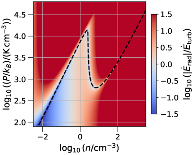
Figure 1: Comparison of energy sources and sinks in thermal gas phase space. Dashed black line shows where the gas is in thermal equilibrium ($\mathcal{L}=0$ in Equation 10). Color map compares net radiative energy change (either loss via cooling or gain via heating) to the total turbulent energy we inject (Equation 9). Three phases (a warm phase, an unstable phase, and a cold phase) with different temperatures can exist in pressure equilibrium for pressures between $P/k_{B}\sim 10^{3}\,\mathrm{K}\,\mathrm{cm}^{-3}$ and $P/k_{B}\sim 10^{4}\,\mathrm{K}\,\mathrm{cm}^{-3}$

The equilibrium curve in pressure-density phase space created by these heating and cooling terms is shown as a black dashed line in Figure 1. Using this radiative cooling and heating setup creates a gas which has two thermally stable phases (with different temperatures) which can exist in pressure equilibrium with each other. There is also a thermally unstable phase in the same pressure range. This bi-stable model of the ISM captures the important physical process of thermal instability (Field, 1965) in its simplest form: the transition between a warm phase and a cold phase.

Figure 1 also shows a colormap comparing the radiative energy rate with the turbulent energy injection rate. The radiative energy rate is calculated by taking the absolute value of $\mathcal{L}(n,T)$ in Equation 11 and multiplying by the simulation volume $L^{3}$, whereas the turbulent energy injection rate is a constant in $(P,n)$ space (see Equation 9). While near thermal equilibrium the turbulent energy injection dominates, its contribution is subdominant in most of the domain (except for the wedge at low densities). Note that the turbulent energy input is given for comparison purposes only; it is not a heating mechanism in the same sense as the photoelectric effect on dust grains. When the only energy gains and losses are those represented by Equation 10, heating dominates below the thermal equilibrium curve and cooling dominates above it.

We start the simulation in thermally stable equilibrium with the gas in the warm phase at a temperature of $6388\,\mathrm{K}$ and a density of $1\,\mathrm{cm}^{-3}$. The turbulent stirring perturbs the gas, compressing some gas into thermally unstable states which then collapse into small scale clouds via the thermal instability.

2.5 Scalar Dye for Dense Gas Formation

Although we do not include self gravity or mass sinks representing star particles in our simulations, we do attempt to track the formation of cold gas which could eventually form stars. We do this by injecting a passive scalar dye at a constant rate $1M_{\odot}\,\mathrm{Myr}^{-1}$ into cells which hit the temperature floor $(T_{\mathrm{floor}}=20\,\mathrm{K})$. This rate comes from assuming a star formation rate of $1M_{\odot}\,\mathrm{yr}^{-1}$ in a galaxy volume of about $10^{12}\,\mathrm{pc}^{3}$, but then adjusting for our simulation volume of $10^{6}\,\mathrm{pc}^{3}$.

The gas density in thermal equilibrium at the temperature floor $T=20\,\mathrm{K}$ is $252\,\mathrm{cm}^{-3}$. For our $N=256^{3}$ simulations, the gas mass in a single cell at that density and temperature is about $3.5M_{\odot}$. The Jeans mass at that density and temperature is about $50M_{\odot}$. Therefore, we would need to produce a contiguous agglomeration of $\sim 15$ cells in order to meet the conditions for gravitational instability.

Another consideration is self-shielding by molecular hydrogen in dense clouds. This effect changes the cooling function and allows more molecular gas to form, which could make it easier for a cloud to gravitationally collapse. Self-shielding becomes important at an atomic hydrogen column density of $N_{H}\sim 5\cdot 10^{20}\,\mathrm{cm}^{-2}$ (Draine, 2011), which corresponds to a number density

$$n_{H}\sim\frac{N_{H}}{R}=162\,\mathrm{cm}^{-3}\frac{N_{H}}{5\cdot 10^{20}\,\mathrm{cm}^{-2}}\frac{L}{1\,\mathrm{pc}}$$ (13)

assuming a cloud of radius $R=1\,\mathrm{pc}$. This effect may therefore become important in the most central regions of any cold gas regions in our simulations. However, we certainly do not resolve these molecular regions, given our resolution of $\Delta x=0.39\,\mathrm{pc}$ in the $256^{3}$ simulations. We do not include their formation or the effect hydrogen self shielding because of this resolution limit.

While we do not simulate star formation, the effects of self gravity, or the formation of molecular gas, the scalar dye traces dense gas formation over the simulation’s evolution. Overall, it allows us to track how much total dense gas is formed in each simulation.

2.6 Two Zone Cosmic Ray Diffusion Coefficient

Our two-zone cosmic ray transport model is motivated by ion-neutral damping (Xu et al., 2016). We assume the cosmic rays are scattered by Alfven waves from an extrinsic turbulent cascade. When the ionization of the ISM decreases in cold clouds, those Alfven waves are damped by collisions between ions and neutrals (Kulsrud & Pearce, 1969; Kulsrud & Cesarsky, 1971), increasing the effective cosmic ray diffusion coefficient in that gas. The effect of an increased diffusion coefficient in cold gas has been examined in the context of global simulations of cosmic ray feedback, where it drastically reduced the coupling between the colder gas and the cosmic rays (Farber et al., 2018).

To implement the temperature dependent cosmic ray energy diffusion coefficient, we adjust the method used in Farber et al. (2018), which used a discontinuous, piecewise constant function for $\kappa$. This prescription produces numerical instability if the discontinuity is too large. To increase numerical stability, we introduce a smooth function for the transition between two values of $\kappa$ in the cold and warm gas; $\kappa_{c}$ and $\kappa_{w}$, respectively.

To allow larger variations in $\kappa$ we build the transition in logarithmic space

$$\log_{10}\kappa(T)=\left(\log_{10}(\kappa_{c})-\log_{10}(\kappa_{w})\right)f_{c}(T)$$

$$+\log_{10}(\kappa_{w})$$ (14)

using a switching function

$$f_{c}(T)=\frac{1}{2}\left(1-\tanh\left(\frac{T-T_{0}}{\Delta T}\right)\right).$$ (15)

This function requires a transition temperature $T_{0}$ between the diffusion coefficient values, along with a transition width $\Delta T$ in temperature. Our implementation allows the diffusion coefficient to change by several orders of magnitude with more numerical stability.

2.7 Parameter Choices

With the implementation of cosmic ray decoupling in Section 2.6, we have several new parameters to set for a simulation of ISM conditions. First, we set the gas density, temperature, plasma beta, and cosmic ray beta which describe the initially homogeneous fluid. Next, we decide on the diffusion coefficients in the warm and cold gas ($\kappa_{w}$ and $\kappa_{c}$ in Equation 14). Finally, we set the parameters of the switching function used to calculate $\kappa$ ($T_{0}$ and $\Delta T$ in Equation 15).

The parameters for each simulation are shown in Table 1. We set the initial plasma parameters as $T_{i}=6388\,\mathrm{K}$, $n=1\mathrm{cm}^{-1}$, $\beta=1$, and $\beta_{\mathrm{cr}}=5$ (in the simulation without cosmic rays, $\beta_{\mathrm{cr}}=\infty$). The choice of $\beta_{\mathrm{cr}}=5$ comes from the assumption that the cosmic ray energy increases with time and the radiative cooling causes thermal energy to decrease with time. Therefore, the $\beta_{\mathrm{cr}}$ should decrease with time. If we want there to be a significant amount of time where the thermal, magnetic, and cosmic ray energy are all a similar order of magnitude (i.e. $\beta_{\mathrm{cr}}\sim 1$), then we have to start with a larger $\beta_{\mathrm{cr}}>1$. An approximate energy equipartition mimics the state of the ISM in the Milky Way, while also allowing us to examine an interesting case.

Simulation	$T_{i}(\mathrm{K})$	$\beta$	$\beta_{\mathrm{cr}}$	$\kappa_{w}(\mathrm{cm}^{2}\,\mathrm{s}^{-1})$	$\kappa_{c}(\mathrm{cm}^{2}\,\mathrm{s}^{-1})$
No CR	$6388$	$1$	$\infty$	-	-
Milky Way	$6388$	$1$	$5$	$3\cdot 10^{28}$	$3\cdot 10^{28}$
Critical	$6388$	$1$	$5$	$5.82\cdot 10^{25}$	$5.82\cdot 10^{25}$
Two Zone	$6388$	$1$	$5$	$5.82\cdot 10^{25}$	$3\cdot 10^{28}$

Table 1: Start-up parameters and cosmic ray energy diffusion coefficients for each simulation. Each of these setups were run at two resolutions $(128,256)$, with a modified speed of light $V_{m}=(1/60,1/30)c$ respectively.

For the diffusion coefficients, we start by considering the measured average value in the Milky Way. The Milky Way cosmic ray diffusion coefficient value of $\kappa_{\mathrm{MW}}\approx 3\cdot 10^{28}\,\mathrm{cm}^{2}\,\mathrm{s}^{-1}$ (Jones et al., 2001; Evoli et al., 2019, 2020) comes from calculations of the grammage (set by the observed ratio of primary and secondary CRs), which we denote by $X$ and which has dimensions of mass per area (Berezinskii et al., 1990). Grammage is a measure of the amount of material a cosmic ray passes through on its path through the ISM. The average diffusion coefficient $\overline{\kappa}$ can be calculated from the grammage using

$$X\approx\rho c\tau=\rho c\frac{L^{2}}{\overline{\kappa}}\hskip 7.22743pt\rightarrow\hskip 7.22743pt\overline{\kappa}=\rho c\frac{L^{2}}{X}.$$ (16)

where $L$ is the root-mean-square displacement of cosmic rays from their source during their confinement time in the Milky Way, $\bar{\rho}$ is the average density of the ISM, and $\tau$ is the average time it takes the cosmic rays to diffuse. Taking displacement to be approximately the thickness of the Milky Way $L\sim 500\,\mathrm{pc}$, mean density to be $\bar{\rho}=m_{p}\,\mathrm{cm}^{-3}$, and $X\sim 10\,\mathrm{g}\,\mathrm{cm}^{-2}$ for the low energy $(\sim 1\,\mathrm{GeV})$ cosmic rays (Evoli et al., 2019), gives an order of magnitude estimate of $\overline{\kappa}\sim 10^{28}\,\mathrm{cm}^{2}\,\mathrm{s}^{-1}\approx\kappa_{\mathrm{MW}}$. A more refined method gives the commonly used $\kappa_{\mathrm{MW}}\approx 3\cdot 10^{28}\,\mathrm{cm}^{2}\,\mathrm{s}^{-1}$.

Another interesting value is the critical diffusion identified in Commerçon et al. (2019); Bustard & Oh (2022, 2023). Near the critical diffusion coefficient the cosmic rays will significantly disrupt the turbulent cascade. Bustard & Oh (2022) use analytical arguments to determine the dependence of the critical rate on various parameters, finding

$$\kappa_{\mathrm{crit}}=0.15v_{\mathrm{ph}}L_{0}=0.15L_{0}\sqrt{\frac{P_{g}+P_{B}+P_{c}}{\rho}}$$

$$=0.15L_{0}\sqrt{\frac{k_{B}T}{m}}\sqrt{1+\beta^{-1}+\beta^{-1}_{\mathrm{cr}}}$$

$$=5.82\cdot 10^{25}\frac{\mathrm{cm}^{2}}{\mathrm{s}}\frac{L_{0}}{100\mathrm{pc}}T_{i}^{1/2}\sqrt{\frac{1+\beta^{-1}+\beta^{-1}_{\mathrm{cr}}}{3}}$$ (17)

where $L_{0}$ is the outer scale of the turbulent cascade, $v_{\mathrm{ph}}$ is the phase velocity of waves, and $0.15$ is a fitted coefficient found by Bustard & Oh (2022) using simulation results.

This diffusion coefficient is too low compared to $\kappa_{\mathrm{MW}}$. If $\kappa_{\mathrm{crit}}$ were the actual diffusion coefficient in the Milky Way, then the grammage would be increased by a factor of $2\cdot 10^{2}$. Even though $\kappa_{\mathrm{crit}}$ is physically unrealistic for an average value in the Milky Way, it is the other diffusion coefficient of interest. In addition to a base simulation without cosmic rays (No CR) we run simulations with constant diffusion coefficients at $\kappa_{\mathrm{MW}}$ and $\kappa_{\mathrm{crit}}$, labelled Milky Way and Critical respectively (see Table 1).

If we allow gas phases to have different diffusion coefficients (see Section 2.6) which contribute to the grammage, then the grammage contributed by each zone (labeled with an integer $i$) would be

$$X_{i}=m_{p}cn_{i}\frac{L_{i}^{2}}{\kappa_{i}}$$ (18)

where we assume the ISM consist of only hydrogen atoms. $L_{i}$ is the size of the region. From this, we can calculate the relative contribution of different regions to the total grammage. If we assume two regions, then their ratio is given by:

$$\frac{X_{1}}{X_{2}}=\frac{n_{1}}{n_{2}}\left(\frac{L_{1}}{L_{2}}\right)^{2}\frac{\kappa_{2}}{\kappa_{1}}.$$ (19)

Assuming the regions were formed following a conserved total number of particles (meaning the number density and length scale of the regions are related $n\propto L^{-3}$), the expression simplifies to

$$\frac{X_{1}}{X_{2}}=\frac{L_{2}\kappa_{2}}{L_{1}\kappa_{1}}.$$ (20)

If two regions contribute equally to the grammage the cosmic rays experience, then the ratio in the characteristic scale of the regions also sets the change in cosmic ray diffusion coefficient between the regions.

For our Two Zone simulation, we use the calculation of $\kappa$ in Equation 14 with a warm diffusion coefficient $\kappa_{w}=\kappa_{\mathrm{crit}}$ and a cold diffusion coefficient $\kappa_{c}=\kappa_{\mathrm{MW}}$. This setup still corresponds to an increased total grammage compared to observations in the Milky Way, if we assume the warm gas is volume filling and that cosmic rays travel through $10\times$ as much of it:

$$\frac{X_{w}}{X_{c}}=\frac{L_{c}\kappa_{c}}{L_{w}\kappa_{w}}\approx\frac{1}{10}\frac{\kappa_{\mathrm{MW}}}{\kappa_{\mathrm{crit}}}\approx 10^{2}.$$ (21)

. However, this model sets up an interesting case where the cosmic rays should adjust dynamics in the warm gas and the formation of cold gas while minimizing their effect on the motion and properties of cold gas clouds.

The Two Zone simulation also allows us to build on Commerçon et al. (2019), who find that cold gas is difficult to form when the cosmic rays become a dominant factor in the dynamics. By allowing cosmic rays to move rapidly through cold regions, we examine an interesting regime where cold gas still forms while cosmic rays adjust the turbulent energy cascade in the warm neutral medium.

In the Two Zone simulation we use we use $1000\mathrm{K}$ for transition temperature $T_{0}$ because it cuts through the middle of the unstable neutral medium. We use a width of $\Delta T=0.1T_{0}$ which is wide enough to allow for smooth transitions and steep enough to limit the number of cells with a diffusion coefficient in between the two constant values.

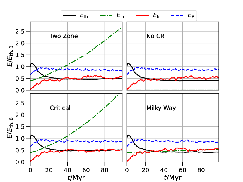
Figure 2: Energy evolution in each simulation. Solid black lines show the total thermal energy, dash-dotted green lines show the total cosmic ray energy, solid red lines show total kinetic energy, and dashed blue lines show total magnetic energy. All energies are normalized by the initial thermal energy. While qualitatively similar, each run has unique characteristics. For example, the Two Zone and Critical simulations both have large increases in cosmic ray energy, but the Two Zone simulation ends up with more kinetic energy later in the simulation.

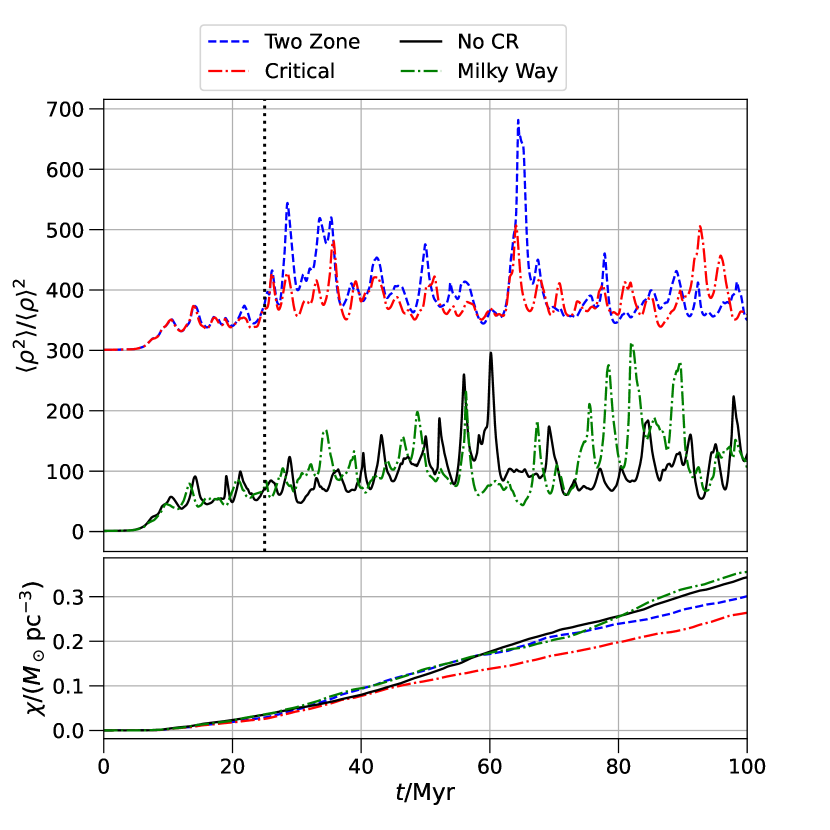
Figure 3: Top plot: Gas density clumping factor (used in Commerçon et al. (2019)) for each simulation. Solid black line shows the No CR simulation, dash-dotted green line shows the Milky Way simulation, dash-dotted red line shows the Critical simulation, and dashed blue line shows the Two Zone simulation. To make the plot clearer, we add $300$ to the clumping factors of the Critical and Two Zone runs. Initially, those two runs track with each other almost exactly. Then, the Two Zone run develops enough cold gas such that the cosmic ray transport differs significantly and more clumps of cold gas form. The Two Zone simulation then reaches clumping factors similar to those in the No CR and Milky Way simulations. Bottom plot: Average value of scalar dye in each simulation (with units of $M_{\odot}\mathrm{pc}^{-3}$, see Section 2.5). The Critical run produces the least amount of scalar dye at all times. The Two Zone simulation tracks with the Milky Way simulation once it has developed cold gas, while the Milky Way and No CR simulations fluctuate near one another for the entire simulation run.

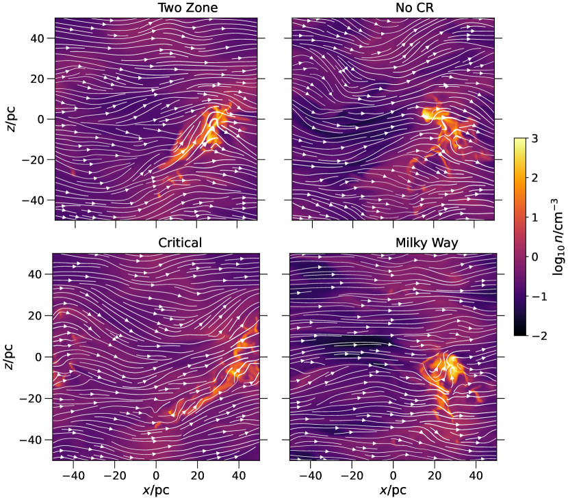
Figure 4: Slices from each simulation showing the gas number density. White lines show the magnetic field, and have a thickness proportional to the strength of the magnetic field (thicker line means stronger field). Each slice is at a time of $t=85\,\mathrm{Myr}$ and at $y=0$. The density colormap is the same for each plot and is shown in the colorbar to the right.

3 Results

In this section we cover our simulations in depth. For a short summary of key takeaways, see Section 5. Each simulation is run for $100\,\mathrm{Myr}$. That time frame allows the turbulent state to saturate and covers $\sim 8$ sound crossing times $\tau_{s}=L_{0}/\sqrt{k_{B}T_{i}/m}\approx 13\,\mathrm{Myr}$. When calculating median quantities in Sections 3.2, 3.5, & 3.4 we set $25\,\mathrm{Myr}$ to be the start of the saturated state and take the median over a time range of $[25,100]\,\mathrm{Myr}$ with data at each $1\,\mathrm{Myr}$. This saturated state after $t=25\,\mathrm{Myr}$ is apparent in Figures 2 and 3. We show results from the $N=256$ simulations, but these results are also apparent in the $N=128$ simulations.

3.1 Energy Evolution

Simulation	$\dot{E}_{\mathrm{rad}}/\dot{E}_{\mathrm{turb}}$	$\dot{E}_{\mathrm{cr}}/\dot{E}_{\mathrm{turb}}$
No CR	$-1.4\pm 0.3$	NA
Milky Way	$-1.5\pm 0.5$	$0.010\pm 0.005$
Critical	$-1.1\pm 0.2$	$0.21\pm 0.07$
Two Zone	$-1.2\pm 0.5$	$0.18\pm 0.06$

Table 2: Time derivatives of radiative energy and cosmic ray energy averaged over the saturated regime from $t=25\,\mathrm{Myr}$ to $t=100\,\mathrm{Myr}$. The standard deviation during that time frame is denoted with a $\pm$. By comparing the net cooling of the four simulations, it is apparent that having cosmic rays transported at the critical rate in warm gas siphons some energy, decreasing the energy lost to optically thin cooling. The Two Zone and Milky Way simulations have the largest variation in radiative energy, likely because of their formation of dense structures (see Section 3.2).

The evolution of thermal, cosmic ray, kinetic, and magnetic energy for each simulation is shown in Figure 2. The compressive driving initially heats the gas (increasing thermal energy) before some of the gas is pushed into a thermally unstable regime and collapses into cold clouds. This collapse leads to a loss of thermal energy as the gas cools via optically thin radiative cooling (see Section 2.4).

The average radiative energy loss rate during the saturated regime is shown in Table 2, normalized by the turbulent energy injection rate in Equation 9. The No CR and Milky Way simulations emit more radiation, on average, than the Critical and Two Zone simulations.

Given the nearly constant loss of radiative energy (see Table 2) along with the steady thermal, kinetic, and magnetic energy (see Figure 2), it is clear that most of the energy injected is radiated away in the No CR and Milky Way simulations. The only difference in the Critical and Two Zone simulation is the steady increase of cosmic ray energy. Since the other energies reach a similar steady state as in the No CR simulation, there must be less radiation in the simulations with cosmic rays transported at the critical diffusion coefficient.

In Figure 2, the cosmic ray energy increases almost linearly in the three simulations which include cosmic rays, but the rate is dependent on the diffusion coefficient. In the Critical and Two Zone simulations, the increase in cosmic ray energy is faster than in the Milky Way simulation. In Table 2, we show the average rate of change of cosmic ray energy over the saturated regime for each simulation. The rate of increase in the Critical and Two Zone simulations is approximately $20\times$ the rate of increase in the Milky Way simulation. This difference is the result of using the critical diffusion coefficient in the warm gas $\kappa_{w}=\kappa_{\mathrm{crit}}$. Because the warm gas is volume filling, $\kappa_{w}$ is the diffusion rate for a majority of the simulation’s volume. With a significant volume near the critical value identified in Bustard & Oh (2022) and Bustard & Oh (2023), there is cosmic ray energization (or reacceleration) which creates a larger energy sink.

The most important part of Figure 2 is the nearly constant values of magnetic, kinetic, and thermal energy from $t=25\,\mathrm{Myr}$ to $t=100\,\mathrm{Myr}$. For each simulation, we do statistical analysis over that time frame to better understand the effect of including cosmic rays. A caveat to this is the increasing cosmic ray energy in the Critical and Two Zone simulations. However, their growth rate is consistent over the same time frame, and is a result of siphoning of energy from the rest of the ISM. The cosmic ray pressure gradients will be the important dynamical factor, and those can stay at the same order of magnitude while the total cosmic ray energy increases.

3.2 Structure Formation

Next, we examine the formation of cold, dense gas in each simulation. Commerçon et al. (2019) use a unitless clumping factor $\langle\rho^{2}\rangle/\langle\rho\rangle^{2}$ to average over the volume of each of their simulations and quantify the appearance of dense structures. We calculate this clumping factor for each of our simulations, and show its evolution over time in Figure 3. The burstiness in time exhibited by the clumping factor highlights the necessity of frequent data dumps from the simulations. The lines in Figure 3 are made up of data points from every $10^{-2}\,\mathrm{Myr}$, as we set the clumping factor to be calculated as part of Athena++ history output.

The No CR and Milky Way simulations initially evolve together and have a larger clumping factor than the Critical and Two Zone simulations. However, as the simulations continue, the Two Zone simulation produces larger clumping factors, close to the values in the No CR and Milky Way simulations. This increase reflects the ability of the Two Zone simulation to create larger dense structures than the Critical simulation. If we label any of the increases in clumping factor as “compressive episodes”, then it is clear that the adjustment of $\kappa$ in cold gas allows higher density structures to form in the Two Zone simulation when compared to the Critical simulation. Because the simulations all use the same random seed to generate turbulence, the Two Zone and Critical simulations have compressive episodes at the same times, but denser clumps are formed in the Two Zone simulation.

Additionally, we show the evolution of the total amount of scalar dye $(\chi)$ (see Section 2.5) in Figure 3. There is no decay or loss mechanism for $\chi$, so it tracks the total amount of cold dense gas produced over the course of each simulation. The Critical simulation produces the least amount of cold dense gas at all times, where as the Two Zone, Milky Way, and No CR simulations cross each other at different points. This crossing is caused by the intermittency of dense cloud formation, which is shown in the time evolution of the clumping factor in top plot of Figure 3. At the end of the simulation, the Two Zone simulation has produced over $20\%$ more cold dense gas than the Critical simulation, and the only difference between those simulations was the increased diffusion coefficient in cold gas.

In Figure 4, we show slices of each simulation at the same positions $(y=0\,\mathrm{pc})$ and time $(t=100\,\mathrm{Myr})$. These slices show the gas density with overlayed magnetic field as white streamlines. The thickness of the lines corresponds to the magnetic field strength at that point. The resolution is large enough to illustrate some of the smaller scale structure within the high density regions. The magnetic field is significantly distorted in the dense structures, where it is also the strongest. Overall, the magnetic field is predominantly in the $\hat{x}$ direction in each simulation.

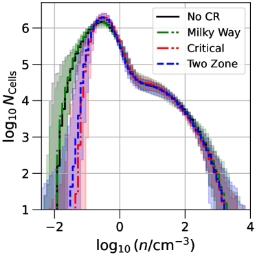
Figure 5: Number density histogram for each simulation. The lines show the median histogram over the entire period of saturation. The shaded regions show the full range of histogram values for each simulation. The No Cr and Milky Way simulation are nearly identical. The Two Zone and Critical simulations are also nearly identical, except the Two Zone simulation has more spread in the low density regime. The Two Zone and Critical simulations both produce less low density warm gas than the Milky Way and No CR simulations.

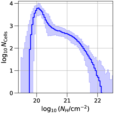
Figure 6: Column density histogram for the Two Zone simulation. The line shows the median histogram over the entire period of saturation. The shaded regions show the full range of histogram values for each simulation. The column density is calculated by integrating along the $\hat{x}$ axis, parallel to the mean magnetic field.

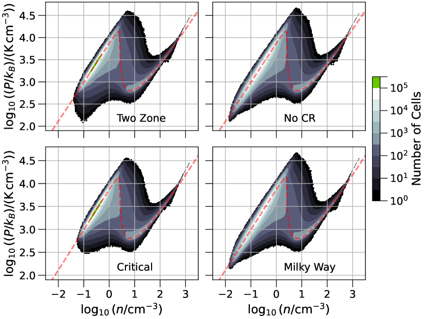
Figure 7: Pressure-Density phase diagrams for each simulation. The histograms illustrate the distribution of gas in phase space and along the thermal equilibrium curve $(\mathcal{L}=0)$, which is shown as a dashed black line. Each diagram uses the same coloring for the contours, which is illustrated in the colorbar to the right of the plots. We take the median of the histograms over the saturated time frame, between $25\,\mathrm{Myr}$ and $100\,\mathrm{Myr}$. The Two Zone and Critical simulations have more warm gas concentrated above a number density of $10^{-1}\,\mathrm{cm}^{-3}$. Overall, the phase diagrams are similar across all the simulations.

3.3 Gas Density & Pressure Phase Space

Next we examine the phase space (gas pressure and number density) of each simulation. In Figure 5 we show the histogram of gas number density for each simulation. Each shaded region corresponds to the full range of histograms for a given simulation, between $t=25\,\mathrm{Myr}$ and $t=100\,\mathrm{Myr}$ with $1\,\mathrm{Myr}$ time steps. Each line shows the median histogram over that time frame. Overall, the No CR and Milky Way simulations match, and the Critical and Two Zone simulations match. The Two Zone and Critical simulations have very little gas below $n=0.1\,\mathrm{cm}^{-3}$, compared to the other simulations.

While the difference is not statistically significant, the Critical simulation has less high density gas, and more thermally unstable gas (near $n=10\,\mathrm{cm}^{-3}$). This change likely results from the gas being more difficult to compress. With the smaller diffusion coefficient in the Critical simulation, the cosmic ray energy will not diffuse away fast enough during compressions. The cosmic ray pressure gradient then builds up and resists the compression.

In Figure 6 we show the distribution of column densities, integrated in the $\hat{x}$ direction along the magnetic field in the Two Zone simulation. The distribution is, overall, similar to the number density histograms in Figure 6. However, $N_{H}$ is an observable and we can compare our distribution to realistic Milky Way column densities $N_{H}\sim 10^{21}\,\mathrm{cm}^{-2}$. Many sightlines along the magnetic field in our simulation do not intersect a cold, dense cloud, meaning most sightlines have lower column densities than expected for the Milky Way. To match the Milky Way’s column densities for a majority of sightlines, we would need to integrate across several realizations of our simulation volume. This point should be kept in mind when evaluating the verisimilitude of the cosmic ray transport model in the Two Zone simulation.

Next, we look at pressure-density phase space. We produce phase space histograms for each $1\,\mathrm{Myr}$ of evolution in the saturated regime, and then we take the median of those histograms to produce a single plot for each simulation. Those median phase space distributions are shown in Figure 7. For each simulation, we also plot the thermal equilibrium curve as a dashed black line. The curve is determined by solving Equation 10 with $\mathcal{L}=0$.

	VFF (%)			MFF (%)
Simulation	Cold	Warm	Unst.	Cold	Warm	Unst.
No CR	$1.6\pm 0.2$	$92\pm 1$	$6\pm 1$	$61\pm 1$	$30\pm 1$	$9\pm 2$
Milky Way	$1.6\pm 0.3$	$93\pm 1$	$6\pm 1$	$60\pm 1$	$30\pm 1$	$9\pm 2$
Critical	$1.6\pm 0.2$	$93\pm 1$	$5\pm 1$	$55\pm 1$	$36\pm 1$	$9\pm 2$
Two Zone	$1.6\pm 0.2$	$93\pm 1$	$5\pm 1$	$56\pm 1$	$35\pm 1$	$9\pm 2$

Table 3: Volume Filling Fraction (VFF) and Mass Filling Fraction (MFF) in each simulation, written as percentages. The quantites are calculated by averaging the MFF and VFF over the saturated time frame. We also provide the standard deviation $(1\sigma)$ of the filling fractions over that $75\,\mathrm{Myr}$ of evolution. The only significant change due to cosmic rays and their transport is in the MFF of cold and warm gas. This change is related to the lower production of cold dense gas shown in Figure 3.

Each simulation’s histogram is visually similar, with large populations of cold and warm gas in the thermally stable regimes of the equilibrium curve. There is more warm gas than cold gas in each simulation. We see the same cutoff of $n\sim 0.1\,\mathrm{cm}^{-3}$ for the Two Zone and Critical simulations which was apparent in the density histograms (Figure 5). We also see the warm gas distribution in the Two Zone simulation extends to lower pressures at that density. This extension was also apparent at low densities in the density histograms, where the Two Zone simulations had slightly more low density gas than the Critical simulation. This extension is unique to the Two Zone simulation, implying it is related to the temperature dependent diffusion coefficient.

The turbulent driving is compressive, creating regions with increased density and pressure. This driving is more apparent in the No CR and Milky Way phase diagrams. The extension toward the top of the phase diagram in these simulations is larger because the cosmic ray energy is taking away less of the injected energy during a compression. In the Two Zone and Critical simulations, the warm gas has the critical diffusion coefficient, allowing the cosmic ray energy to serve as a sink for some of the injected turbulent energy, reducing the amount of compression which takes place.

Finally, in Table 3, we show the volume filling fractions (VFFs) and mass filling fractions (MFFs) of the different gas phases in each simulation. The listed quantities are percentages, and they are calculated by taking the average over the saturated regime. The listed errors are the standard deviation during the $75\,\mathrm{Myr}$ time frame. Overall, the simulations all have the same VFF for each phase. The only impact cosmic rays have is on the MFF of cold and warm gas. This decrease in cold gas MFF (and corresponding increase in warm gas MFF) is likely tied to the lower total amount of cold gas formation over the course of the simulation (see scalar dye evolution in Figure 3).

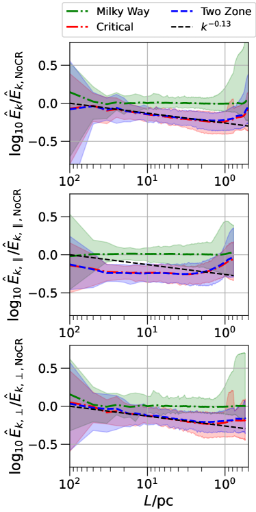
Figure 8: Kinetic energy per mass spectra from the Milky Way, Critical, and Two Zone simulations compared to the No CR simulation’s spectrum. Lines show the median spectrum, whereas the shaded regions show the full variation of the spectrum over the saturated timeframe. Top plot: The total kinetic energy per unit mass shows the Milky Way simulation produces the same cascade as the No CR simulation. However, the Two Zone and Critical simulations have a steeper spectrum by a factor of $k^{-0.13}$. Middle plot: The kinetic energy per unit mass parallel to the mean magnetic field is decreased at all scales in the Critical and Two Zone simulations. Bottom plot: The kinetic energy per unit mass perpendicular to the mean magnetic field has the same spectral change as the total spectrum for the Critical and Two Zone simulations.

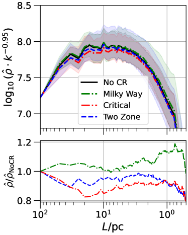
Figure 9: Top plot: Fourier transform (spectrum) of gas density for each simulation, scaled by a power law of $k^{0.95}$. The lines are the median spectrum, whereas the shaded regions show the full variation over the saturated time frame. While the spectra are relatively similar, there is less dense gas at all scales in the Critical simulation. The Two Zone and Milky Way simulations have the largest variations in their spectrum. Bottom plot: The ratio of other simulations’ median spectrum to the No CR simulation spectrum. The overall profiles of each simulation are consistent, but the Critical and Two Zone simulations have less dense gas at small scales, whereas the Milky Way simulation has more dense gas than the No CR simulation at small scales.

Simulation	Kinetic Energy Slope ($\alpha$ in $k^{-\alpha}$)
No CR	$1.78\pm 0.07$
Milky Way	$1.77\pm 0.07$
Critical	$1.92\pm 0.08$
Two Zone	$1.90\pm 0.07$

Table 4: Average inertial range spectral index for each simulation with $1\sigma$ variations. The dependence on $\kappa_{w}$ is clear, as simulations Critical and Two Zone have a steeper slope and are the simulations with cosmic ray energy diffusion at the critical rate $\kappa_{\mathrm{crit}}$ through the warm gas. Steepening of the spectrum as a result of cosmic ray transport matches results from Bustard & Oh (2023) even though we have added radiative cooling. Additionally, the slope of our No CR run is similar to the slope of the equivalent run in Bustard & Oh (2023).

3.4 Power Spectra

To study the effect of the cosmic ray energy on the saturated turbulence, we examine how the power spectrum of kinetic energy varies between each simulation. In Figure 8, we plot the total kinetic energy per mass $(v^{2}/2)$ spectrum, the spectrum parallel to the mean magnetic field (meaning. the $\hat{x}$ direction, so $v_{x}^{2}/2$), and the spectrum perpendicular to the mean magnetic field. The solid lines correspond to the median spectrum over the saturated time frame and the shaded regions show the full variation. We divide the spectra from the Milky Way, Critical, and Two Zone simulations by the median spectrum from the No CR simulation.

We also calculate the original slope of each spectrum’s inertial range, and these are listed in Table 4. For each $1\,\mathrm{Myr}$ time dump, we fit a power law $k^{-\alpha}$ over the length scales $L\in[5,20]\,\mathrm{pc}$. We then average the power law index $\alpha$ over the saturated time frame to get the average slope values and their $1\sigma$ variation.

The transport of cosmic ray energy at the critical diffusion coefficient steepens the spectral slope, similar to some results in Bustard & Oh (2023), even though our simulations have multiple gas phases. The change in slope is approximately $k^{-0.13}$.

We also examine the anisotropy of the kinetic energy cascade. The kinetic energy per mass in the direction parallel to the magnetic field is reduced at all scales in the inertial range. In the perpendicular direction, we see the same change in spectral slope as in the total kinetic energy per mass.

In Figure 9 we show the Fourier transform of the gas density in each simulation, along with the ratio of cosmic ray simulation to the No CR simulation. Overall, the simulations produce the same characteristic density spectrum, with a power law $k^{-0.95}$ in the inertial range $(L\in[5,20]\,\mathrm{pc})$. However, the Two Zone and Milky Way simulations have larger variation, particularly at scales near $2.5\,\mathrm{pc}$. The variation in the spectrum is apparent in the gas density clumping factor shown in Figure 3, where the Milky Way simulation has a higher clumping factor than even the No CR simulation, along with more cold gas production (larger $\chi$).

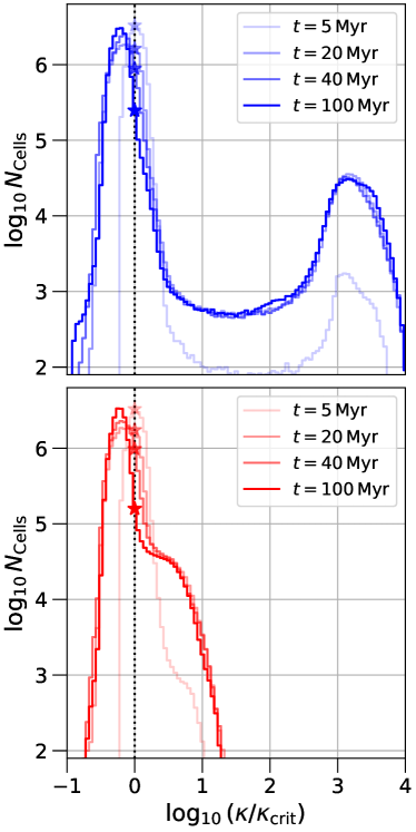
Figure 10: Histograms of $\kappa/\kappa_{\mathrm{crit}}$ for the Two Zone (top plot, blue lines) and Critical (bottom plot, red lines) simulations. At each cell, we calculate $\kappa_{\mathrm{crit}}$ from Equation 17 using the cell’s pressure and density values. We then take the actual diffusion coefficient in that cell and divide by the local critical coefficient. The histograms are shown at several times, and stars mark where $\kappa=\kappa_{\mathrm{crit}}$. Even as the total cosmic ray energy increases in these two simulations (see Figure 2), there is still a significant portion of the simulation volume where diffusion occurs at the critical rate.

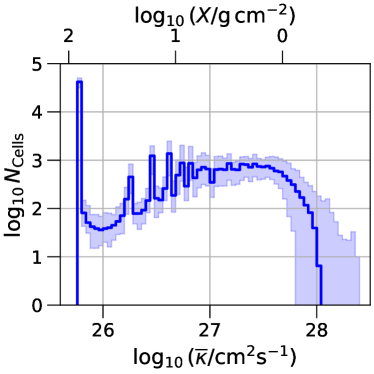
Figure 11: Distribution of average diffusion coefficient along the mean magnetic field (in the $\hat{x}$ direction) in the Two Zone Simulation. The solid line is the median distribution, and the shaded region shows the full variation over the saturated time frame. A majority of paths through the simulation do not intersect a cloud of cold gas because that phase only fills $\sim 2\%$ of the volume, so a majority of paths have the warm gas diffusion coefficient $\kappa_{\mathrm{crit}}$ on average. However, over $1\%$ of the paths have an average diffusion coefficient greater than $10^{27}\,\mathrm{cm}^{2}\mathrm{s}^{-1}$ because they pass through cold gas where the diffusion coefficient jumps to $3\cdot 10^{28}\,\mathrm{cm}^{2}\mathrm{s}^{-1}$

3.5 Diffusion Coefficient Statistics

In Figure 10, we show histograms of the ratio of the cosmic ray energy diffusion coefficient $\kappa$ (calculated from Equation 14) to the local critical diffusion coefficient $\kappa_{\mathrm{crit}}$ (calculated at each cell using Equation 17) for the Two Zone and Critical simulations. The blue lines in the upper plot are from the Two Zone simulation whereas the red lines in the lower plot are from the Critical simulation. Stars mark the value of the histogram at $\kappa=\kappa_{\mathrm{crit}}$ and in both plots the stars move down with increasing time. This decrease in the amount of gas with cosmic ray transport at the critical rate is the result of increasing cosmic ray energy in the simulations (see Figure 2). As the cosmic ray energy increases, the critical diffusion coefficient $\kappa_{\mathrm{crit}}$ increases. This increase leaves a majority of the gas with a diffusion coefficient below the critical value.

In Figure 11 we show a histogram of average diffusion coefficients. The diffusion coefficients are averaged over the $\hat{x}$ direction of the simulation, leaving $256^{2}=65536$ paths. A majority of the paths travel only through warm gas and keep the original critical diffusion coefficient value. However, nearly $1\%$ of all the paths actually end up with a diffusion coefficient above $10^{27}\,\mathrm{cm}^{2}\,\mathrm{s}^{-1}$. Those diffusion coefficients correspond to more realistic grammage values $X$ (see Section 2.7) which are shown across the top of the plot. Our estimate of a change in grammage by a factor of $10^{2}$ (see Equation 21 in Section 2.7) appears reasonable given this distribution.

Figure 11 is a lower limit on the distribution of average diffusion coefficient $\overline{\kappa}$ and grammage $X$. Using mass-weighted average or actual path integration along the magnetic field, the paths would pass through more cold gas because there is some bending in the field lines (see Figure 4). This change in paths would cause more gas at low grammage and high diffusivity because more magnetic field lines pass through the cold gas where the field strength is large. Additionally, our lines of integration do not pass through as much of the ISM as cosmic rays in the Milky Way (see column density histogram in Figure 6). If every path passed through a cold cloud, then there would be many more paths with a realistic mean diffusion coefficient $\overline{\kappa}$ and grammage $X$.

4 Discussion

This section roughly follows the order of results presented in Section 3. For our final conclusions and summary, see Section 5.

Figure 2 together with Table 2 show that when cosmic rays are weakly coupled or not present at all, the system reaches a steady state with turbulent energy input balanced by compression and radiative cooling. When strongly coupled cosmic rays are added to the mix, as in the Critical and Two Zone simulations, some turbulent energy input goes into compressive heating of cosmic rays. In that case, less of the turbulent energy input is lost to radiative cooling.

However, there is rarefaction as well as compression, and one might ask why the cosmic rays gain energy instead of returning it back to the flow during rarefaction. A full answer to this question is beyond the scope of the present paper and we plan to address it in future work. However, we provide a partial answer by considering how cosmic ray diffusion affects small amplitude acoustic waves.

Consider the linearized cosmic ray pressure equation for waves propagating along the ambient magnetic field:

$$\partialderivative{\delta P_{c}}{t}=-\gamma_{c}P_{c}\partialderivative{\delta v}{x}+\kappa\partialderivative[2]{\delta P_{c}}{x}.$$ (22)

Assume the solution is a plane wave with frequency $\omega$ and wavenumber $k$. Cosmic rays do work on the gas at the rate $\dot{E}=-\delta v\partial\delta P_{c}/\partial x$ (note $E$ refers to energy density, not energy). Using the linearized equation to determine $\delta P_{c}$ in terms of $\delta v$ allows us to calculate the energy change

$$\dot{E}=-\gamma_{c}P_{c}|k\delta v|^{2}\frac{\kappa k^{2}}{\omega^{2}+\kappa^{2}k^{4}}.$$ (23)

Equation (23) shows that cosmic rays steadily extract energy from the wave, much as a gas which conducts heat extracts energy from sound waves. The effect is maximized at $\omega/k=\kappa k$. If we identify $\omega/k$ with the phase velocity and $k$ with $L^{-1}$ we recover the argument used to estimate the critical diffusivity $\kappa_{\mathrm{crit}}$ (see Equation 17) in Bustard & Oh (2022).

This effect has a counterpart in the kinetic theory description of cosmic ray propagation in the limit of short mean free path Skilling (1975). It is akin to first order Fermi acceleration because the cosmic rays are scattering off converging fluctuations, due to the advection of the fluctuations by the mean flow.

Returning to the effect of cosmic rays on compressive turbulence, we see that during the formation of dense gas, the cosmic rays can diffuse independently of the gas, quickly redistributing energy from compressed regions. Those dense regions can collapse further because any cosmic ray pressure gradients have been decreased or removed. This process is clearest in the evolution of the gas density clumping factor and scalar dye $\chi$ in Figure 3. We see the Two Zone, Milky Way, and No CR simulations have large spikes and variation in clumping as opposed to the evolution in the Critical simulation where cosmic rays provide significant pressure support against the formation of cool clouds. While cool clouds still form in the Critical simulation, there are fewer of them and they do not reach as high densities, which is clear from the Critical simulation’s smaller production of scalar dye $\chi$. This process agrees with the results presented in Commerçon et al. (2019), which showed that decreasing the diffusion coefficient leads to smoother gas distributions and fewer cold clouds.

The Two Zone simulation also allowed us to examine how a temperature dependent diffusion coefficient would affect the grammage cosmic rays pass through on their way through the ISM. Observations of the primary-to-secondary ratio give stringent requirements on the grammage $X$ that $\mathrm{GeV}$ cosmic rays will experience on average (Evoli et al., 2019, 2020). In our Two Zone simulation, the cosmic rays mainly experience a grammage set by the volume filling warm gas. However, Figure 11 shows that some paths will have physically realistic grammage values when just the cold gas has a realistic diffusion coefficient. Additionally, most paths through the simulation do not produce a realistic column density (see Figure 6). Performing the integration over multiple realizations of the simulation box would produce more sightlines with higher column densities. Those higher column density sightlines would also have a higher average diffusion coefficient $\overline{\kappa}$.

Therefore, for Milky Way column densities, the diffusion coefficient in the cold gas could become the dominant contributor to the mean cosmic ray diffusion coefficient. This conclusion adds to the importance of cosmic ray transport modelling which accounts for changes in temperature, ionization, or magnetic field strength. For example, in the realistic case of the diffusion coefficient in the warm gas and cold gas being $\kappa\sim\kappa_{\mathrm{MW}}$, the diffusion coefficient in hot and warm ionized gas could be a much lower value (possibly near $\kappa_{\mathrm{crit}}$) without changing the average cosmic ray diffusion coefficient calculated from the observed primary-to-secondary ratio.

While not a physically significant result, we find that the numerical stability of the Two Zone simulation depends on how we calculated the diffusion coefficient. Applying the switching function in logarithmic space leads to a smoother transition in regions with a large temperature gradient. This may be useful for other studies which model inhomogeneous diffusion without the added computational expense of calculating $\kappa$ ab initio and on the fly from gas parameters.

We show the cosmic ray diffusion coefficient has a significant impact on the turbulent cascade in Section 3.4. This results from a simple relationship in the original CR+MHD equations. A rapid flattening and smoothing of cosmic ray pressure, caused by a large diffusion coefficient, minimizes the effect of cosmic rays because there is less time for the pressure gradient $\gradient P_{c}$ to change the motion of gas (Equation 3). A smaller diffusion coefficient means large peaks in the cosmic ray pressure can exist longer and create large pressure gradients which adjust the gas flow.

The steepening of the kinetic energy spectrum by a factor of $k^{-0.13}$ in Figure 8 is clearly the result of the critical diffusion coefficient in the warm gas because the same results appear for simulations Critical and Two Zone. The reduction in parallel kinetic energy at all scales is because of the decreased diffusion parallel to the magnetic field, i.e. the $\kappa\nabla^{2}E_{c}$ term contained in the $\divergence{\mathbf{F_{c}}}$ term of Equation 5. The lower diffusion coefficient means there is enough time for the turbulent flows to drive more energization before the cosmic rays diffuse away.

The steepening in spectral slope for the perpendicular (and total) kinetic energy is more difficult to physically explain. If the $k^{-1.84}$ dependence in simulation No CR is the result of our turbulent driving being too strong to develop a Kolmogorov $(k^{-5/3})$ or Iroshnikov-Kraichnan $(k^{-3/2})$ spectrum, then the further adjustment towards Burgers turbulence $(k^{-2})$ suggests transport at the critical diffusion coefficient may increase the frequency of ‘shocks’ in the direction perpendicular to the magnetic field. Although, we see little to no formation or propagation of shocks. Instead, it is possible the sharp density discontinuities between the cold and warm phases have an effect on turbulent transport similar to that of shocks in Burgers turbulence (instantaneous transfer of energy from large to small scales rather than a true cascade).

A secondary point from the examination of the kinetic energy spectra is that the slope of the No CR run is similar to the slope found in Bustard & Oh (2023), despite our inclusion of optically thin radiative cooling. This similarity is likely because motions on inertial scales $(20\,\mathrm{pc}>L>5\,\mathrm{pc})$ are mostly determined by the warm gas in our simulations. This warm gas follows an equation of state similar to the simple adiabatic law in Kritsuk et al. (2017) & Bustard & Oh (2023). To see the differences created by radiative cooling, we would need to extend the inertial scale below $5\,\mathrm{pc}$. This extension requires increasing the resolution of our simulations. However, an increase in resolution will make our treatment of diffusive transport of $E_{c}$ inaccurate (see Section 2.1). This limitation highlights the importance of future simulations which evolve the cosmic ray distribution function and/or actual particle trajectories (e.g. using methods like MHD-PIC, Sun & Bai 2023).

5 Conclusions

We presented simulations of a bi-stable ISM including the effects of cosmic ray feedback for three different cosmic ray diffusion coefficient models, along with a simulation with no cosmic ray energy. We used a long baseline for statistical analysis of the saturated turbulent state. We showed that cosmic rays can decrease the amount of energy radiated away via optically thin cooling. This energy siphoning is mediated by a process similar to first order Fermi acceleration in regions with a non-zero divergence of the velocity field. We illustrated the impacts of a temperature dependent (as a proxy for ionization dependence) cosmic ray diffusion coefficient on the formation of cold dense gas and cosmic ray grammage. We re-examined the adjustment of the turbulent energy cascade by cosmic rays detailed in Bustard & Oh (2022, 2023) and find the cosmic rays have an anisotropic effect on the cascade.

From these simulations, our analysis, and our discussion, the key conclusions are:

1. Cosmic ray transport at the critical rate allows cosmic rays to remove energy from collapsing gas via first order Fermi acceleration, decreasing the total radiated energy (see Table 2).

2. Increasing the diffusion coefficient only within cold gas allows $\sim 20\%$ more cold, dense gas to form than in a simulation with a constant diffusion coefficient (see Figure 3).

3. Even when the volume filling warm gas has a small diffusion coefficient, over $1\%$ of paths through our simulation box have an average grammage set by the diffusion coefficient in cold gas (see Figure 11). Given that the cold gas is not volume filling and our column densities are low (see Figure 6), we underestimate the number of paths through the ISM with an average diffusion coefficient set by the diffusion coefficient in cold gas.

4. Cosmic ray energy transported via diffusion at the critical rate identified in Bustard & Oh (2023) decreases kinetic energy parallel to the mean magnetic field at all scales by nearly a factor of $2$, while also changing the spectral slope of kinetic energy perpendicular to the mean magnetic field by a factor of $k^{-0.13}$ (see Figure 8).

References

- Astropy Collaboration et al. (2013) Astropy Collaboration, Robitaille, T. P., Tollerud, E. J., et al. 2013, A&A, 558, A33, doi: 10.1051/0004-6361/201322068
- Astropy Collaboration et al. (2018) Astropy Collaboration, Price-Whelan, A. M., Sipőcz, B. M., et al. 2018, AJ, 156, 123, doi: 10.3847/1538-3881/aabc4f
- Berezinskii et al. (1990) Berezinskii, V. S., Bulanov, S. V., Dogiel, V. A., & Ptuskin, V. S. 1990, Astrophysics of cosmic rays
- Bustard & Oh (2022) Bustard, C., & Oh, S. P. 2022, ApJ, 941, 65, doi: 10.3847/1538-4357/aca021
- Bustard & Oh (2023) —. 2023, arXiv e-prints, arXiv:2301.04156, doi: 10.48550/arXiv.2301.04156
- Bustard & Zweibel (2021) Bustard, C., & Zweibel, E. G. 2021, ApJ, 913, 106, doi: 10.3847/1538-4357/abf64c
- Commerçon et al. (2019) Commerçon, B., Marcowith, A., & Dubois, Y. 2019, A&A, 622, A143, doi: 10.1051/0004-6361/201833809
- De La Torre Luque et al. (2023) De La Torre Luque, P., Gaggero, D., Grasso, D., et al. 2023, A&A, 672, A58, doi: 10.1051/0004-6361/202243714
- Desiati & Zweibel (2014) Desiati, P., & Zweibel, E. G. 2014, ApJ, 791, 51, doi: 10.1088/0004-637X/791/1/51
- Draine (2011) Draine, B. T. 2011, Physics of the Interstellar and Intergalactic Medium
- Eswaran & Pope (1988) Eswaran, V., & Pope, S. B. 1988, Computers and Fluids, 16, 257
- Evoli et al. (2019) Evoli, C., Aloisio, R., & Blasi, P. 2019, Phys. Rev. D, 99, 103023, doi: 10.1103/PhysRevD.99.103023
- Evoli et al. (2020) Evoli, C., Morlino, G., Blasi, P., & Aloisio, R. 2020, Phys. Rev. D, 101, 023013, doi: 10.1103/PhysRevD.101.023013
- Farber et al. (2018) Farber, R., Ruszkowski, M., Yang, H. Y. K., & Zweibel, E. G. 2018, ApJ, 856, 112, doi: 10.3847/1538-4357/aab26d
- Field (1965) Field, G. B. 1965, ApJ, 142, 531, doi: 10.1086/148317
- Guo et al. (2016) Guo, Y.-Q., Tian, Z., & Jin, C. 2016, ApJ, 819, 54, doi: 10.3847/0004-637X/819/1/54
- Harris et al. (2020) Harris, C. R., Millman, K. J., van der Walt, S. J., et al. 2020, Nature, 585, 357, doi: 10.1038/s41586-020-2649-2
- Hunter (2007) Hunter, J. D. 2007, Computing in Science and Engineering, 9, 90, doi: 10.1109/MCSE.2007.55
- Inoue et al. (2006) Inoue, T., Inutsuka, S.-i., & Koyama, H. 2006, ApJ, 652, 1331, doi: 10.1086/508334
- Iroshnikov (1964) Iroshnikov, P. S. 1964, Soviet Ast., 7, 566
- Jiang & Oh (2018) Jiang, Y.-F., & Oh, S. P. 2018, ApJ, 854, 5, doi: 10.3847/1538-4357/aaa6ce
- Jóhannesson et al. (2019) Jóhannesson, G., Porter, T. A., & Moskalenko, I. V. 2019, ApJ, 879, 91, doi: 10.3847/1538-4357/ab258e
- Jones et al. (2001) Jones, F. C., Lukasiak, A., Ptuskin, V., & Webber, W. 2001, ApJ, 547, 264, doi: 10.1086/318358
- Kolmogorov (1941) Kolmogorov, A. 1941, Akademiia Nauk SSSR Doklady, 30, 301
- Kraichnan (1965) Kraichnan, R. H. 1965, Physics of Fluids, 8, 1385, doi: 10.1063/1.1761412
- Kritsuk et al. (2017) Kritsuk, A. G., Ustyugov, S. D., & Norman, M. L. 2017, New Journal of Physics, 19, 065003, doi: 10.1088/1367-2630/aa7156
- Kulsrud & Pearce (1969) Kulsrud, R., & Pearce, W. P. 1969, ApJ, 156, 445, doi: 10.1086/149981
- Kulsrud & Cesarsky (1971) Kulsrud, R. M., & Cesarsky, C. J. 1971, Astrophys. Lett., 8, 189
- Matthaeus et al. (2003) Matthaeus, W. H., Qin, G., Bieber, J. W., & Zank, G. P. 2003, ApJ, 590, L53, doi: 10.1086/376613
- Pingel et al. (2018) Pingel, N. M., Lee, M.-Y., Burkhart, B., & Stanimirović, S. 2018, ApJ, 856, 136, doi: 10.3847/1538-4357/aab34b
- Pingel et al. (2022) Pingel, N. M., Dempsey, J., McClure-Griffiths, N. M., et al. 2022, PASA, 39, e005, doi: 10.1017/pasa.2021.59
- Ptuskin (1988) Ptuskin, V. S. 1988, Soviet Astronomy Letters, 14, 255
- Ruszkowski & Pfrommer (2023) Ruszkowski, M., & Pfrommer, C. 2023, A&A Rev., 31, 4, doi: 10.1007/s00159-023-00149-2
- Shalchi et al. (2006) Shalchi, A., Bieber, J. W., Matthaeus, W. H., & Schlickeiser, R. 2006, ApJ, 642, 230, doi: 10.1086/500728
- Skilling (1975) Skilling, J. 1975, MNRAS, 172, 557, doi: 10.1093/mnras/172.3.557
- Stone et al. (2020) Stone, J. M., Tomida, K., White, C. J., & Felker, K. G. 2020, The Astrophysical Journal Supplement Series, 249, 4, doi: 10.3847/1538-4365/ab929b
- Sun & Bai (2023) Sun, X., & Bai, X.-N. 2023, MNRAS, 523, 3328, doi: 10.1093/mnras/stad1548
- Uhlenbeck & Ornstein (1930) Uhlenbeck, G. E., & Ornstein, L. S. 1930, Physical Review, 36, 823, doi: 10.1103/PhysRev.36.823
- van der Walt et al. (2011) van der Walt, S., Colbert, S. C., & Varoquaux, G. 2011, Computing in Science and Engineering, 13, 22, doi: 10.1109/MCSE.2011.37
- Wiener et al. (2017) Wiener, J., Oh, S. P., & Zweibel, E. G. 2017, MNRAS, 467, 646, doi: 10.1093/mnras/stx109
- Xu et al. (2016) Xu, S., Yan, H., & Lazarian, A. 2016, ApJ, 826, 166, doi: 10.3847/0004-637X/826/2/166
- Yan & Lazarian (2008) Yan, H., & Lazarian, A. 2008, ApJ, 673, 942, doi: 10.1086/524771
- Zweibel (2013) Zweibel, E. G. 2013, Physics of Plasmas, 20, 055501, doi: 10.1063/1.4807033
- Zweibel (2017) —. 2017, Physics of Plasmas, 24, 055402, doi: 10.1063/1.4984017