Abstract

Entezari et al. (2022) conjectured that neural network solution sets reachable via stochastic gradient descent (SGD) are convex, considering permutation invariances. This means that two independent solutions can be connected by a linear path with low loss, given one of them is appropriately permuted. However, current methods to test this theory often fail to eliminate loss barriers between two independent solutions (Ainsworth et al., 2022; Benzing et al., 2022). In this work, we conjecture that a more relaxed claim holds: the SGD solution set is a star domain that contains a star model that is linearly connected to all the other solutions via paths with low loss values, modulo permutations. We propose the Starlight algorithm that finds a star model of a given learning task. We validate our claim by showing that this star model is linearly connected with other independently found solutions. As an additional benefit of our study, we demonstrate better uncertainty estimates on Bayesian Model Averaging over the obtained star domain. Code is available at https://github.com/aktsonthalia/starlight.

1 Introduction

The learning problem for a neural network is inherently non-convex. This is characterized by a non-convex loss landscape, leading to multiple possible solutions rather than a singular one. Efforts to comprehend this landscape and the set of solutions have been ongoing.

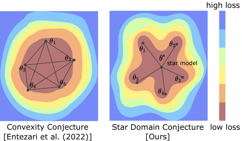
Figure 1: A schematic view of the loss landscape modulo permutations, à la the convexity conjecture Entezari et al. (2022) vs the star domain conjecture (ours).

A significant early discovery in this area was made by Garipov et al. (2018), who demonstrated that almost any two independent solutions could be connected through a simple curve comprising sequences of solutions. This finding highlighted the vastness of the solution space in neural-network-based learning problems.

While mode connectivity has illuminated the vastness of the solution set, other research has focused on its complexity. Entezari et al. (2022) explored the permutation symmetries in the parameter space. For example, linear weights and neuron positions may be jointly swapped without changing the function represented by the neural network Entezari et al. (2022); Singh & Jaggi (2021); Ainsworth et al. (2022); Guerrero Peña et al. (2023). They proposed that when accounting for these symmetries, the solution set found by the stochastic gradient descent (SGD) essentially becomes convex. This convexity conjecture suggests that any pair of independent solutions can be linearly connected through a low-loss line segment, assuming an appropriate permutation is found for one of the models.

However, this conjecture has faced challenges. Subsequent studies (Juneja et al., 2022; Benzing et al., 2022; Ainsworth et al., 2022; Altintas et al., 2023; Guerrero Peña et al., 2023) revealed that even after the application of permutation-finding algorithms, two distinct solutions in the parameter space might still be separated by a high-loss region, which we refer to as a high loss barrier. These studies attribute this discrepancy to various factors, including width (Ainsworth et al., 2022) and high learning rates (Altintas et al., 2023).

In response to these findings, our research introduces the star domain conjecture. We propose that solutions in deep neural networks (DNNs), when permutations are taken into account, form a star domain rather than a convex set. A star domain is a set $A$ with at least one special element, known as a star point, $a_{0}\in A$ that is connected to every other element in $A$. See Figure 1 for an illustration.

This star domain conjecture represents a relaxed version of the convexity conjecture, as a convex set is a specific instance of a star domain. This adjustment in hypothesis lets us avoid conflicts with the previously mentioned contradictory findings. The star domain conjecture is still a stronger assertion than mode connectivity which states that any two models can be connected by two line segments through a third point in the parameter space: $\forall\theta_{A},\theta_{B}\in\Theta$, $\exists\theta_{C}$ such that $(\theta_{A},\theta_{C})$ and $(\theta_{B},\theta_{C})$ are linearly connected. Our conjecture essentially implies that all pairs of solutions are interconnected via a shared third solution, the star point, which is common to all solution pairs: $\exists\theta_{C}$ such that $\forall\theta_{A},\theta_{B}\in\Theta$, $(\theta_{A},\theta_{C})$ and $(\theta_{B},\theta_{C})$ are linearly connected

We substantiate our star domain conjecture with empirical evidence. We introduce the Starlight algorithm to identify a candidate star model for a given learning task. Starlight finds a model that is linearly connected with a finite set of independent solutions. We demonstrate that the identified star model candidates are linearly connected to an arbitrary set of solutions that were not used in constructing the star model candidates. This establishes the existence of star models that are linearly connected with other solutions in the solution set, substantiating the star domain conjecture.

In addition to validating the conjecture, our research delves into the distinctive characteristics of star models. We found that sampling from the star domain for Bayesian Model Averaging (BMA) leads to better uncertainty estimates than ensembles. These differences highlight the potential advantages of star models in various neural network applications.

We summarise our contributions:

1. The star domain conjecture, as an alternative to the convexity conjecture, for characterizing neural network solution sets.

2. Starlight for identifying a star model for a gradient-based learning task.

3. Analysis of practical benefits shown by the star models.

2 Related Work

We introduce the relevant development of conjectures and findings in the understanding of solution sets of deep neural networks.

Theory of Mode Connectivity. Garipov et al. (2018) and Draxler et al. (2018) concurrently discovered mode connectivity. Gotmare et al. (2018) soon followed, showing that non-linear mode connectivity can be achieved even between neural networks which were obtained using different training schemes. Kuditipudi et al. (2019) explained mode connectivity through properties like dropout stability and noise stability. Benton et al. (2021) went on to show that neural networks are connected not only via simple paths, but that there also exist volumes of low loss, connecting several solutions. However, they focus on non-linear connectivity, while our focus is on a stricter condition, viz., linear connectivity.

Model Mechanisms and Permutation Invariance. Lubana et al. (2023) investigated the relationship between Linear Mode Connectivity and Model Mechanisms in Image Classification tasks. Juneja et al. (2022) carried out a similar analysis in Natural Language Processing (NLP) tasks. Entezari et al. (2022) proposed that SGD solution sets are convex modulo permutations, while Ainsworth et al. (2022); Guerrero Peña et al. (2023) introduced ”re-basin” methods, i.e., methods which bring different solutions into the same basin. One of these methods viz., weight matching, complements our methods throughout this work.

Practical Applications. Mode connectivity has found applications in model fusion Garipov et al. (2018); Singh & Jaggi (2021), adversarial robustness Zhao et al. (2020); Wang et al. (2023), continual learning Mirzadeh et al. (2020); Wen et al. (2023), and federated learning Ainsworth et al. (2022). In contrast, our work focuses on understanding the surface of the loss landscape. However, we also explore potential applications, e.g., Bayesian Model Averaging.

3 The Star Domain Conjecture

In this section, we state and validate our main claim. We start with some background on the convexity conjecture in Section 3.1. In Section 3.2, we formally state the conjecture that solution sets of deep neural networks are star domains. Next, we introduce Starlight, a tool for verifying the conjecture (Section 3.3), and finally present experimental results obtained using Starlight in Section 3.4.

3.1 Background: The Convexity Conjecture

Here, we provide a formal statement of the convexity conjecture. We start with basic notations. A neural network is a function $f_{\theta}(\cdot)$ parameterized by $\theta\in\Theta$, where $\Theta$ is the parameter space. Given a dataset $\mathcal{D}$, we formulate a non-negative loss $\mathcal{L}(\theta)=\mathcal{L}\left(\theta;\mathcal{D}\right)\geq 0$ and solve a minimization problem to find a solution in $\Theta$. The solution set at threshold $\tau$ is defined as $S_{\tau}:=\{\theta\mid\mathcal{L}\left(\theta\right)<\tau\}$ for some small $\tau>0$.

The loss barrier (Entezari et al., 2022) between two points in the parameter space, $\theta_{A},\theta_{B}\in\Theta$, is defined as:

$$B\left(\theta_{A},\theta_{B}\right):=\max_{t\in[0,1]}\widetilde{\mathcal{L}}_{t}(\theta_{A},\theta_{B})$$ (1)

where

$$\widetilde{\mathcal{L}}_{t}(\theta_{A},\theta_{B}):= \,\,\mathcal{L}\left((1-t)\cdot\theta_{A}+t\cdot\theta_{B}\right)$$

$$-\left((1-t)\cdot\mathcal{L}\left(\theta_{A}\right)+t\cdot\mathcal{L}\left(\theta_{B}\right)\right)$$ (2)

is the difference between the loss value at $t$, and the linear interpolation of the losses at the end-points.

Two solutions $\theta_{A},\theta_{B}\in\Theta$ are said to be linearly mode-connected, or LMC (Frankle et al., 2020), when their loss barrier is below a threshold $\tau>0$: $B\left(\theta_{B},\theta_{A}\right)\leq\tau$.

We now define key ingredients for stating the convexity conjecture. The conjecture is constructed upon a parameter space where the permutation symmetries are factored out. We define permutation invariance as an equivalence relation $\sim$ between two points $\theta_{A},\theta_{B}$ in the parameter space such that $\theta_{A}\sim\theta_{B}$ iff there exists a permutation $\pi$ such that $\pi(\theta_{A})=\theta_{B}$ and the functions represented by them are identical: $f_{\theta_{A}}(x)=f_{\theta_{B}}(x)$ for all $x$.

Given two points $\theta_{A}$ and $\theta_{B}$, we look for the permutation invariance that connects the two points with as low a loss barrier as possible. A winning permutation (Entezari et al., 2022) for models $\theta_{A}$ and $\theta_{B}$ is defined as

$$\underset{\theta_{A}\rightarrow\theta_{B}}{\pi}:=\operatorname*{arg\,min}_{\pi\in\mathcal{P}_{\theta_{A}}}B\left(\pi(\theta_{A}),\theta_{B}\right)$$ (3)

where $\mathcal{P}_{\theta}:=\{\pi\,|\,\pi(\theta)\sim\theta\}$ is the set of all function-preserving permutations of $\theta$.

We are ready to introduce the convexity conjecture formally.

Conjecture 1.

Convexity Conjecture (Entezari et al., 2022). Let $S{}$ be a solution set for a deep neural network. Let $\theta_{A},\theta_{B}\in S{}$ be two solutions. Then, $\theta_{A}$ and $\theta_{B}$ are linearly mode-connected modulo permutation invariances. That is,

$$B\left(\underset{\theta_{A}\rightarrow\theta_{B}}{\pi}(\theta_{A}),\theta_{B}\right)<\tau$$ (4)

for some small $\tau>0$ independent of $\theta$. In other words, the line segment between $\underset{\theta_{A}\rightarrow\theta_{B}}{\pi}(\theta_{A})$ and $\theta_{B}$ is included in $S$.

We refer to this as the convexity conjecture, because by definition, a convex set is precisely a set where the line segment between any two elements is included in the set. The conjecture provides a geometric intuition that the shape of the solution set is generally convex, modulo permutation invariances (Figure 1).

No theoretical result supports the validity of the conjecture beyond a limited setting, given a sufficiently wide network. There are only empirical validations, but such explorations are also performed in a limited setup, achieving perfectly zero barriers only under ideal conditions. Subsequent validations exhibit mixed accounts, with a handful of counterexamples against the convexity conjecture. Ainsworth et al. (2022) notably achieve zero barrier between two ResNet-20-32 models trained on CIFAR-10, but report failure to eliminate the loss barrier between narrower models, even after weight matching. Benzing et al. (2022) provide interesting insights using their activation-matching permutation algorithm. On the one hand, fully connected networks (FCNs) live in the same loss valley even at initialization. On the other hand, convolutional nets are usually not connected even after considering permutation invariances, especially when high learning rates are used. Guerrero Peña et al. (2023) introduce Sinkhorn re-basin, a differentiable permutation-finding approach, however, even with two-layer NNs, the barrier between CIFAR-10 models, albeit low, remains non-zero, while for convolutional architectures like VGG11, the barrier is substantially high. Altintas et al. (2023) show using experiments on MLPs that aggravating factors for LMC include the Adam optimizer, absence of warmup, and complexity of the learning task.

Hence, while being simple and attractive, the convexity conjecture has faced several counterexamples. In this paper, we argue that the convexity conjecture is overly strong and propose a weaker version that does not contradict the findings above.

3.2 The Star Domain Conjecture

We propose a weaker version of the convexity conjecture for characterizing the solution set of deep neural networks. We argue that the solution sets are generally star domains, modulo invariant permutations. We start with the necessary definitions to make a formal description of the conjecture.

A set $A\subset\mathbb{R}^{n}$ is a star domain if there exists an element $a_{0}\in A$ such that for any other element $a\in A$ and $0\leq t\leq 1$, $(1-t)\cdot a_{0}+t\cdot a\in A$. That is, all points on the line segment between $a_{0}$ and $a$ lie in $A$. We call such $a_{0}$ a star point. In the context of the parameter space, we refer to the star point of a star-domain solution set as a star model.

Conjecture 2.

Star Domain Conjecture. Given a solution set $S{}$ for deep neural networks trained to execute a certain machine learning task, there exists a star model $\theta^{\star}\in S{}$ such that for any other solution $\theta\in S{}$,

$$B\left(\underset{\theta\rightarrow\theta^{\star}}{\pi}(\theta),\theta^{\star}\right)<\tau$$ (5)

for some small $\tau>0$ independent of $\theta$. In other words, the line segment between $\underset{\theta\rightarrow\theta^{\star}}{\pi}(\theta)$ and $\theta^{\star}$ is included in $S{}$.

A convex set is a special case of a star domain, where all the elements are star points. Star domain conjecture is thus a relaxation of the convexity conjecture. A notable feature of a star domain is the existence of special elements, star points, that are linearly connected with all the other members of the set. In Section 4, we delve into the characteristics of such star models in $S{}$.

3.3 Finding a Star Model

We provide empirical evidence for the star domain conjecture via two steps. First, we present a method for finding a star model. Second, we verify that the model found is indeed a star model: it has a low loss barrier with an arbitrary solution in $S{}$. Here, we focus on the first step.

Algorithm 1 Starlight: Training a Star Model.

  Input: dataset $\mathcal{D}=\{(x_{i},y_{i})\}_{i=1}^{I}$, source models $Z=\{\theta_{1},\theta_{2},\ldots,\theta_{N}\}$, initial model $\theta_{0}$, learning rate $\lambda$, number of batches $m$, number of steps $K$.

  Step 0. $\theta\leftarrow\theta_{0}$

  for $k=1$ to $K$ do

     if $k\mod m=0$ then

        for $n=1$ to $N$ do

           Step 1. Update $\theta_{n}\leftarrow\underset{\theta_{n}\rightarrow\theta}{\pi}(\theta_{n})$.

        end for

     end if

     Step 2a. Sample $\theta_{n}\sim\text{Unif}(Z)$

     Step 2b. Sample $t\sim\text{Unif}[0,1]$.

     Step 2c. Sample a batch $\mathcal{B}$ from $\mathcal{D}$.

     Step 2d. Compute loss $\mathcal{L}((1-t)\cdot\theta+t\cdot\theta_{n}\,;\,\mathcal{B})$.

     Step 2e. Compute gradients $v\leftarrow\nabla_{\theta}\mathcal{L}((1-t)\cdot\theta+t\cdot\theta_{n})$.

     Step 2f. Update $\theta\leftarrow\theta-\lambda(1-t)\cdot v$

  end for

  Output: $\theta$

To find a star model, we focus on a necessary condition for a model to be a star model $\theta^{\star}$: given an arbitrary set of models $Z=\{\theta_{1},\theta_{2},\dots,\theta_{N}\}$, $\theta^{\star}$ has to be connected to all of them, modulo permutation invariances. We present a recipe for finding a model that is linearly connected to all members of $Z$ simultaneously.

We first obtain a finite set $Z=\{\theta_{1},\theta_{2},\dots,\theta_{N}\}$ of models, independently trained with different random seeds controlling the initialization and batch composition. We then formulate a loss function for $\theta$ that encourages low loss barriers between $\theta$ and some permuted versions of $\{\theta_{1},\theta_{2},\dots,\theta_{N}\}$.

The objective may be expressed as

$$\theta^{\star}_{Z}=\operatorname*{arg\,min}_{\theta}\frac{1}{N}\sum\limits_{\theta_{n}\in Z}B\left(\theta,\underset{\theta_{n}\rightarrow\theta}{\pi}(\theta_{n})\right)$$ (6)

where $\underset{\theta_{n}\rightarrow\theta}{\pi}$ is the winning permutation defined in Section 3.1 that permutes $\theta_{n}$ without changing the represented function while minimizing the loss barrier against $\theta$.

To solve the optimization problem, we propose to minimize the expected loss on the linear interpolation between the model in question $\theta$ and each source model $\theta_{n}$, accounting for permutation invariances. We modify the training objective as

$$\theta^{\star}_{Z}=\operatorname*{arg\,min}_{\theta}\widetilde{\mathcal{L}}_{Z}(\theta)$$ (7)

where

$$\widetilde{\mathcal{L}}_{Z}(\theta):=\frac{1}{N}\sum_{n=1}^{N}\int_{0}^{1}\mathcal{L}\left((1-t)\cdot\theta+t\cdot\underset{\theta_{n}\rightarrow\theta}{\pi}(\theta_{n})\right)dt$$

This expresses the expected loss on the set of line segments between $\theta$ and $\underset{\theta_{n}\rightarrow\theta}{\pi}(\theta_{n})$, where each source model $\theta_{n}\sim\text{Unif}(Z)$ is chosen at random and then each point on the line segment is sampled from $t\in\text{Unif}[0,1]$.

The optimization problem in Equation 7 involves a computational challenge: $\underset{\theta_{n}\rightarrow\theta}{\pi}$ assumes access to the winning permutation. However, the winning permutation depends on $\theta$, which is also the variable being optimized and is, therefore, constantly changing. We introduce the following solutions.

CIFAR10
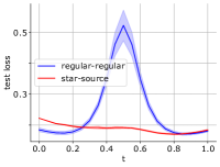
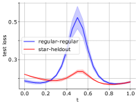
CIFAR100
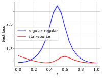
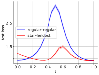
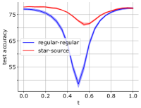
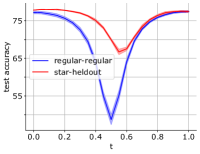
	star $\theta^{\star}$ - source $Z$	star $\theta^{\star}$ - heldout $H$	star $\theta^{\star}$ - source $Z$	star $\theta^{\star}$ - heldout $H$
	Test loss		Test accuracy

Figure 2: Loss barriers for star models. We interpolate between a star model $\theta^{\star}$ and regular models that are trained with SGD. There are two types of regular models, depending on whether they are used for finding the star model: source models $Z$ are used and heldout models $H$ are not. Along the interpolation, we visualise the loss barrier by plotting the test loss and accuracy values (red curves). For these curves, $t=0$ corresponds to the star model $\theta^{\star}$. As a reference curve, we plot the interpolation between two arbitrary regular models (blue curves). The error bands correspond to one standard deviation.

Finding optimal permutations.

We perform weight matching, i.e., we look for a permutation $\pi_{n}$ that maximizes the dot product $\theta{}\cdot\pi_{n}(\theta_{n})$, for each $\theta_{n}\in Z$ Ainsworth et al. (2022). This procedure aligns each source model $\theta_{n}$ with the candidate star model $\theta$. This operation is performed at the beginning of every epoch instead of every iteration, speeding up the optimisation process significantly.

Monte-Carlo optimization scheme.

Instead of estimating $\widetilde{\mathcal{L}}_{Z}(\theta)$ precisely at every iteration, we rely on a Monte-Carlo estimation scheme, inspired by the parameter-curve fitting method by Garipov et al. (2018). At iteration $k\geq 1$, we sample $\theta_{n^{(k)}}$ uniformly from $Z$ and $t^{(k)}$ from $\text{Unif}[0,1]$. Hence, we obtain a single point on the manifold, calculate the cross-entropy loss at this point, and subsequently the gradients for updating $\theta$.

$$\operatorname*{arg\,min}_{\theta}\mathcal{L}\left((1-t^{(k)})\cdot\theta+t^{(k)}\cdot\underset{\theta_{n}\rightarrow\theta}{\pi}(\theta_{n^{(k)}})\right)$$ (8)

Algorithm 1 describes the detailed procedure. Once we find a $\theta$ that has a low expected loss $\widetilde{\mathcal{L}}_{Z}(\theta)$ on the linear paths to a finite set of source models $Z$, we may verify if this $\theta$ is likewise linearly connected with an arbitrary solution $\theta_{N+1}\notin Z$.

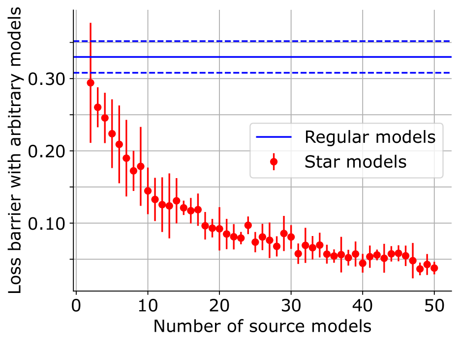
(a) ResNet18-CIFAR10

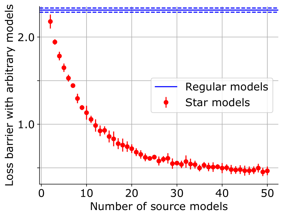
(b) ResNet18-CIFAR100

Figure 3: Starness of a star model vs #source models. We plot the test loss barriers $B(\theta^{\star},\theta_{h})$ between star models $\theta^{\star}$ and heldout models $\theta_{h}\in H$ at different amounts of source models $Z$ used for learning the star model $\theta^{\star}$ (red plots). The heldout set is disjoint with the source models: $H\cap Z=\emptyset$. We provide a reference point given by the test loss barrier between two regular solutions $B(\theta_{A},\theta_{B})$ for $\theta_{A},\theta_{B}\in S{}$ (blue plots). The error bars indicate one standard deviation across five held-out models $|H|=5$. Incorporating a greater number of source models $|Z|$ enables finding a better star model with a lower loss barrier against an arbitrary solution.

3.4 Empirical Evidence

We have introduced Starlight to find a candidate star model. In this section, we propose a method for verifying if the model found in Section 3.3 is a star model.

To verify that a model $\theta$ is a star model, we check whether it is linearly connected to an arbitrary solution $\theta_{N+1}\notin Z$, i.e., not part of the source models used for finding the star model. We refer to such models as held-out solutions $H$ that are disjoint from the source models: $H\cap S=\emptyset$

We present our empirical verification of the star domain conjecture using a ResNet18 image classifier He et al. (2016) trained on the CIFAR10 and CIFAR100 datasets. We set the number of source models, $|Z|=50$, and the number of held-out models, $|H|=5$. All models were trained using standard recipes detailed in Appendix A. We summarize our observations below.

Convexity conjecture does not hold. In Figure 2, we show loss barriers between two independently trained solutions (blue “regular-regular” curves). We observe that the loss increases significantly and accuracy drops significantly at around $t=0.5$, even after applying the algorithm to find the winning permutation. We present another piece of evidence that the convexity conjecture does not hold for thin ResNets, reconfirming the findings of Ainsworth et al. (2022).

Star model has low loss barriers with other solutions. In Figure 2, we show the test losses and test accuracies along the linear path between various types of model pairs. We show the values along the path between the candidate star model $\theta^{\star}$ and other types of solutions (either source models $Z$ or held-out models $H$). They are indicated with red curves. As a reference, we always plot the confidence interval of loss and accuracy values along the line segments between two regular solutions (blue curves). We observe that, for the test loss, star-to-regular connections enjoy essentially zero loss barriers, in contrast with regular-to-regular connections, which remain significantly higher at $0.32$, for CIFAR-10. This demonstrates that it is possible to find a model $\theta^{\star}$ connected to $|Z|=50$ models simultaneously. The same is true for the line segments between the star model $\theta^{\star}$ and a held-out model picked from $|H|=5$ models; although the barrier between the star model and the heldout model is non-zero, it remains as low as $0.03$ compared to $0.32$ for the regular-to-regular case.

A greater number of source models enhances “starness”. Our star model is constructed from the set of source models $Z$. We question whether incorporating more source models increases the likelihood of the star model being linearly connected to other independent solutions. In other words, we question whether greater $|Z|$ induces greater “starness” of the solution found by Starlight. In Figure 3, we plot the loss barrier against the number of source models $2\leq|Z|\leq 50$ used to construct the star model. For statistical significance, we have included the loss barrier statistics between two regular, independently trained models in $S$ and included error bars indicating one standard deviation. We observe that the loss barriers between these star models and the held-out models decrease as $|Z|$ increases. This shows that incorporating more source models in Starlight increases the likelihood of finding a better star model that is connected to more solutions with lower loss barriers. We also note that the decreasing trend has not saturated after $|Z|=50$. We stopped there as we were limited by the available computational resources. However, including more source models is likely to enhance the connectivity between the obtained star model and the other solutions even further.

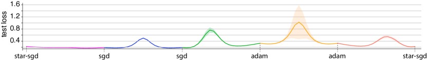
Figure 4: Loss landscape across SGD models, Adam models, and SGD-induced star models. We plot test loss across different types of solutions in $S$. Our star model $\theta^{\star}$ (“star-sgd” in the plot) is constructed from a set of SGD-trained models $Z$. We note that the star model is well-connected with SGD solutions. There exists a loss barrier between the star model and Adam solutions, but the barrier is significantly lower than the barrier among Adam solutions.

Table 1: $\ell_{2}$ distances between different types of model pairs. We compute the mean over 5 source models $Z$ and 5 held-out models $H$.

Pair type	w/o perm	w/ perm
Regular – regular	$30.7\pm 0.19$	$28.2\pm 0.37$
Star $\theta^{\star}$ – heldout $H$	$29.7\pm 0.18$	$26.8\pm 0.45$
Star $\theta^{\star}$ – source $Z$	$29.8\pm 0.08$	$26.8\pm 0.07$

Star models are slightly closer to arbitrary solutions than the latter among each other. Loss barriers measure the connectivity between solutions; we question whether the great connectivity is attributable to the metric closeness of the solutions. We measure the $\ell_{2}$ distances between different types of model pairs. Table 1 shows the distance statistics. We observe that the distances between star $\theta^{\star}$ and source $Z$ or heldout $H$ models tend to be slightly smaller than between two arbitrary solutions (29.7 or 29.8 versus 30.7 without permutation). The difference is slightly greater when considering the winning permutation (“w/ perm”). Albeit small, the difference is statistically significant. This result shows that star models tend to be slightly closer to any solution in $S{}$, but the difference is too small to significantly contribute to the lower loss barrier seen in previous results.

Connectivity to Adam-trained solutions. Throughout the study, we have focused on the SGD-trained solutions and the star model built from SGD-trained source models. We consider a different class of solutions that are trained with the Adam optimiser Kingma & Ba (2014) and examine the connectivity between SGD solutions, SGD-induced star models and the Adam-based solutions. Figure 4 shows the loss landscape across different types of solutions. We observe, as before, the loss barrier between SGD solutions and our star model $\theta^{\star}$ is nearly non-existent, while the SGD solutions are generally not linearly connected. Our star model $\theta^{\star}$ shows less connectivity with Adam solutions (the curve between “adam” and “star-sgd”) than with SGD solutions. However, we note that the loss barrier is significantly lower than for the linear interpolations between pairs of Adam solutions (the curve between “adam” and “adam”). Based on the observation, we conclude that the scope of our conjecture remains within SGD-trained solutions, but there are hints that our star model shows enhanced connectivity with other types of solution subsets.

Caveats. Despite the promising observations above, our star domain conjecture is not theoretically validated and thus remains a conjecture. Also, from the empirical perspective, loss barriers between the star model and other solutions often yield values that are significantly greater than zero. However, we emphasise that this paper is focused on providing the lower bound in evidence supporting the star domain conjecture. Considering a larger number of source models for the star model construction, improving Starlight, and developing a better algorithm for finding the winning-permutations will potentially contribute to the discovery of better star models in the solution set.

Conclusion. Convexity conjecture has faced many counterexamples; our experimental results provide an additional counterexample: a high loss barrier between two arbitrary solutions even after applying the best invariant permutation. We provide a relaxed version, the star domain conjecture. Through empirical validations, we have verified that the star model found through Starlight is likely to be a true star model. Our analysis sheds light on a novel viewpoint on the geometry of the solutions set. We invite the community to expand upon our findings and converge towards a more accurate understanding of the loss landscape.

4 Practical Applications

The star domain conjecture introduces a novel dichotomy of solution types: star models and non-star models. Vast majority of the solutions are not star: they are not linearly connected with other solutions. However, in Section 3, we have presented strong evidence for the existence of star models. In this section, we examine the properties of star models and their potential benefits in practice. Section 4.1 considers whether star models and the surrounding star domain provide a better posterior for Bayesian Model Averaging. In Section 4.2, we introduce the star models as another practical approach to model ensembling.

Table 2: Model fusion performances. Regular models indicate single models; Ensemble indicates a vanilla average of the probability vectors across the member models; Star model is the model found using Starlight using the models as the source set $Z$. ResNet18 has been used throughout. We show one standard deviation for the error bars.

Dataset      #Models		Regular models	Ensemble	Star model
	$2$	$95.2\pm 0.03$	$95.8$	$95.3\pm 0.16$
CIFAR-10	$5$	$95.1\pm 0.14$	$96.0$	$95.2\pm 0.15$
	$50$	$95.1\pm 0.16$	$96.3$	$95.3\pm 0.20$
	$2$	$77.3\pm 0.16$	$79.6$	$78.0\pm 0.24$
CIFAR-100	$5$	$77.4\pm 0.21$	$80.4$	$78.1\pm 0.02$
	$50$	$77.3\pm 0.28$	$81.3$	$78.4\pm 0.10$
Train / test complexity		$\mathcal{O}(1)/\mathcal{O}(1)$	$\mathcal{O}(n)/\mathcal{O}(n))$	$\mathcal{O}(n)/\mathcal{O}(1)$

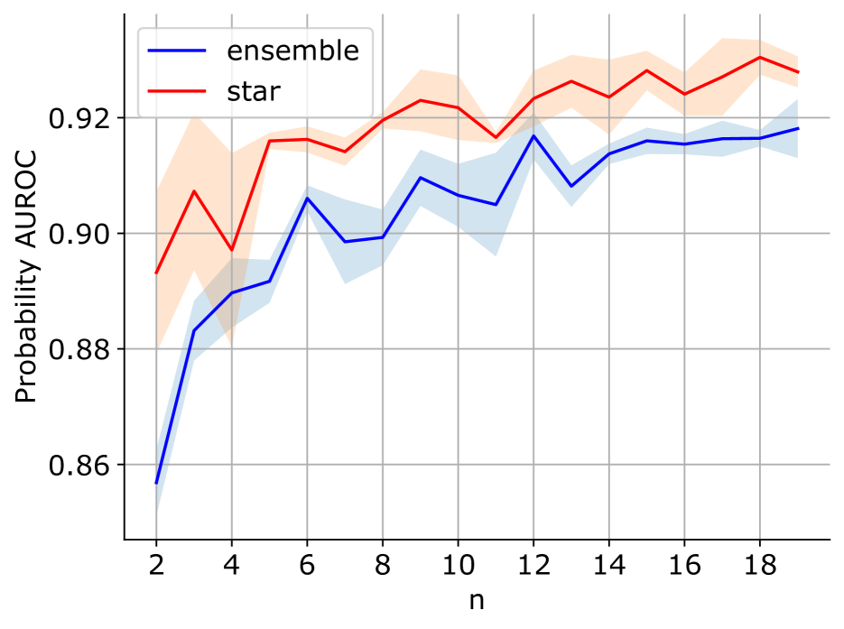
(a) AUROC (Max. Probability)

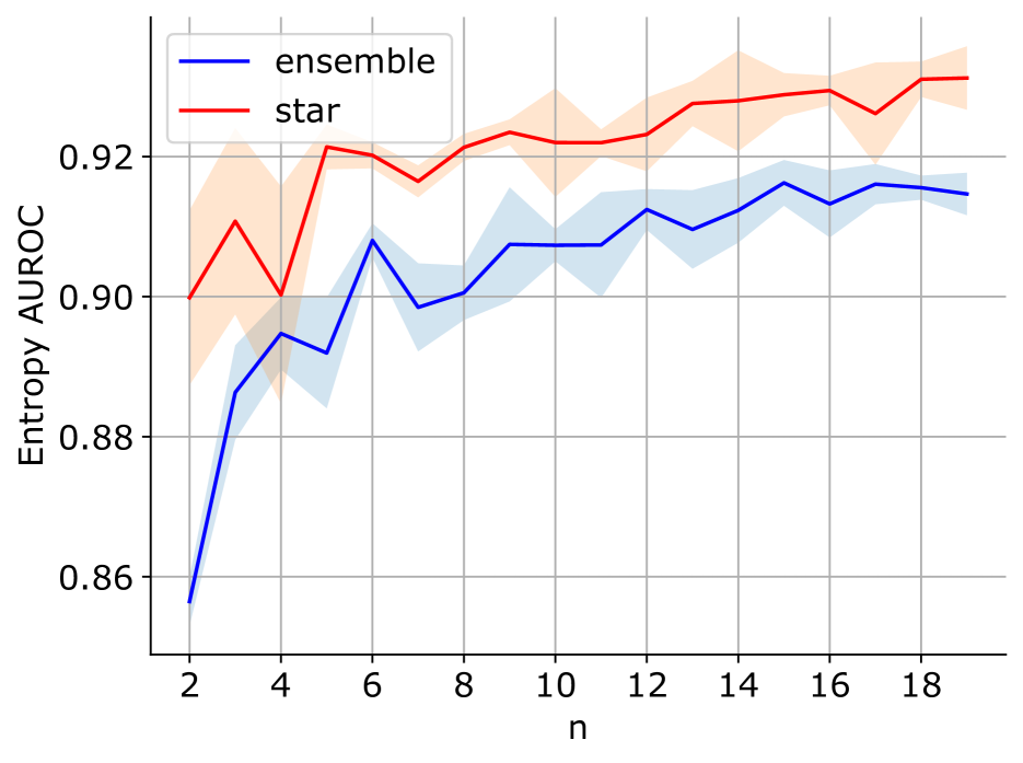
(b) AUROC (Entropy)

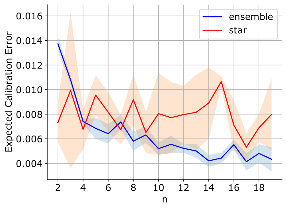
(c) ECE

Figure 5: Bayesian model averaging. The star model was trained using 50 source models. The x-axis denotes the number of models sampled from the star domain for Bayesian model averaging or from the set of source models.

4.1 Bayesian Model Averaging

Bayesian model averaging (BMA) enhances uncertainty estimation by averaging predictions from the posterior of models in the parameter space. Researchers have studied different types of posterior families, ranging from simple Gaussian (Blundell et al., 2015) and Bernoulli (Gal & Ghahramani, 2016) distributions to more complex geometries like splines (Garipov et al., 2018) and simplices (Benton et al., 2021). Here, we examine if the star domain provides a good posterior family for BMA-based uncertainty estimation.

Setup. The posterior of interest is the collection of line segments between the star model $\theta^{\star}$ and other solutions $\{\theta_{1},\cdots,\theta_{N}\}$ that are independently found. As in the Monte-Carlo procedure for Starlight in Equation 8, we sample first from the model index of $\{1,\cdots,N\}$ uniformly and then sample from the line segment $\text{Unif}[0,1]$. As in standard BMA, we consider a set of models sampled from the posterior and the post-softmax average of these models. We use ResNet-18 models trained on CIFAR-10. As a baseline, we present the BMA for the independent solutions $\{\theta_{1},\cdots,\theta_{N}\}$.

Evaluation. We assess the predictive uncertainty of the BMA-based confidence estimates. For the ranking metric, we use the area under ROC curve (AUROC) for the correctness prediction. We consider both max-probability and entropy-based confidence measures. We also show results based on the expected calibration error (ECE).

Results. Figure 5 shows the assessment of the uncertainty quantification at different numbers of posterior samples from 2 to 20. BMA using the star domain posterior consistently exhibits significantly better AUROC values than the baseline deep-ensemble estimates. In terms of ECE, however, the exact calibration is worse than the deep ensemble BMA. The star domain posterior provides avenues for more precisely ranked uncertainty estimates, albeit the exact, absolute-value uncertainty quantification may not be precise.

Conclusion. As an additional benefit of the star domain conjecture, we have studied a novel type of posterior family. We have shown that the star domain posterior provides better uncertainty estimates than the deep ensemble baseline, in terms of the rank-based predictive uncertainty evaluation.

4.2 Potential Usage in Model Fusion

Given a fixed amount of training data, a popular approach to maximize the model generalizability is to fuse predictions from multiple independent models. Also known as ensembles, this basic approach suffers from computational complexities not only during training but also at inference. Every input has to be processed by individual member models at test time. Having to store multiple models also leads to a higher memory footprint which scales linearly with the number of ensemble members. Our star model can also be understood as a method for aggregating multiple source models $Z=\{\theta_{1},\cdots,\theta_{N}\}$ into a single model $\theta^{\star}$. From a computational perspective, star models reduce the necessary time and storage complexity at the inference time. We investigate whether the star models provide an enhanced generalization compared to the individual models.

Setup. We slightly modify the training objective of Starlight to align it with a better generalization capability of the star model. We add a cross-entropy term for the star model:

$$\mathcal{L}_{\text{total}}(\theta,Z)=\widetilde{\mathcal{L}}_{Z}(\theta)+\mathcal{L}\left(\theta\right)$$ (9)

where $\widetilde{\mathcal{L}}_{Z}(\theta)$ is the original optimization objective for the star model discovery in Equation 7.

Evaluation. We evaluate the test accuracies for star models trained using different numbers of source models, $|Z|$. For comparison, we report the test accuracies for ensembles over the same source models.

Results. Results are presented in Table 2. We observe that the star models consistently perform better than regular models (78.4$\%$ versus 77.3$\%$ for CIFAR-100 with $|Z|=50$). Although they are worse in accuracy than ensembles of their corresponding source models, they only use a fraction of the compute during inference.

Conclusion. We have shown that “starness” of a solution may aid its generalization. Depending on the application scenario, where test-time inference costs matter a lot, star models may provide a promising alternative to vanilla ensembles.

5 Conclusion

This paper proposes a novel understanding of SGD loss landscapes. The traditional picture before Garipov et al. (2018), was one of extreme non-convexity, in contrast with the current picture of near-perfect convexity in a canonical, modulo-permutations space Entezari et al. (2022). Our claim paints a more realistic picture between the two extremes: that the solution set is a star domain modulo permutations. Our empirical findings support this hypothesis. We propose the Starlight algorithm to find candidate “star models” and verify that they are indeed linearly connected to other solutions. In addition to the empirical evidence for the star domain conjecture, we present potential use cases for star models in practice, including uncertainty estimation through Bayesian model averaging and model fusion.

Acknowledgments. This work was supported by the German Federal Ministry of Education and Research (BMBF): Tübingen AI Center, FKZ: 01IS18039A. The authors would also like to thank Arnas Uselis and Bálint Mucsányi for helpful insights.

Appendix A Implementation Details

This section describes the finer details of our experiments.

Handling batch normalization. Most conventional neural networks use batch normalization Ioffe & Szegedy (2015) for speed and stability of convergence. However, batch normalization in interpolated models poses a variance collapse problem Jordan et al. (2023). However, in order to make sure that our findings are relevant in practice, we still make use of batch-normalized networks. As a solution to the variance collapse problem, we recalculate the batch statistics for each interpolated model by making one pass over the entire training set Garipov et al. (2018).

Hyperparameters. ResNet-18 models on CIFAR-10 and CIFAR-100 were trained using SGD with momentum $0.9$ and a weight decay of $5e-4$. We set the initial learning rate to $0.1$ and gradually reduced it to zero over the course of 200 epochs, via cosine decay. We used a batch size of $128$ and standard augmentations (padding by 4 pixels followed by cropping from the image or its horizontal mirror).

Appendix B Additional Results

Our experiments on CIFAR using ResNet models provide empirical validation toward the star domain hypothesis. In order to further support our claim, we also test another architecture (DenseNet-40-12 Huang et al. (2018)) and dataset (ImageNet-1k Deng et al. (2009)). We present the results here.

DenseNet-40-12 on CIFAR.

In Figure 6, we present a comparison of the interpolations between regular models, and interpolations between the star models and regular models, all of which are DenseNets trained on CIFAR-10 and CIFAR-100. Despite observing higher loss barriers across the board, a consistent trend emerges, supporting the star domain conjecture (Figure 6). The star model was trained using $50$ source models. We posit that the weaker trend is an artifact of higher model complexity and we hypothesize that expanding the source model count could effectively diminish the loss barriers, aligning better with 2.

ResNet18 on ImageNet.

In order to determine whether our conjecture also holds true in large-scale settings, we trained $30$ ResNet18 models on ImageNet-1k, from scratch. Subsequently, we trained a star model and observed the loss barriers. We present the results in Figure 7. The increased complexity of the dataset in this case poses a more difficult problem in identifying an optimal star model. Consistent with findings from CIFAR-trained models, we speculate that an increase in the source model quantity could bolster already available evidence.

CIFAR10
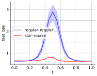
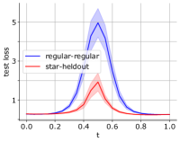
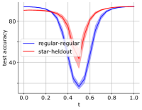
CIFAR100
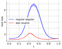
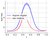
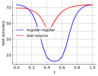
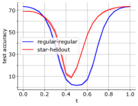
	star $\theta^{\star}$ - source $Z$	star $\theta^{\star}$ - heldout $H$	star $\theta^{\star}$ - source $Z$	star $\theta^{\star}$ - heldout $H$
	Test loss		Test accuracy

Figure 6: Loss barriers for star models (DenseNet). For details on interpreting the figures, see Figure 2.

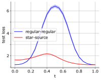
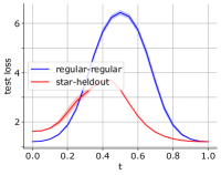
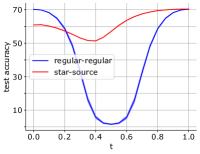
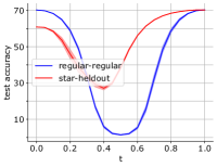
star $\theta^{\star}$ - source $Z$	star $\theta^{\star}$ - heldout $H$	star $\theta^{\star}$ - source $Z$	star $\theta^{\star}$ - heldout $H$
Test loss		Test accuracy

Figure 7: Loss barriers for star models (ImageNet). For details on interpreting the figures, see Figure 2.

References

- Ainsworth et al. (2022) Ainsworth, S. K., Hayase, J., and Srinivasa, S. Git Re-Basin: Merging Models modulo Permutation Symmetries, December 2022. URL http://arxiv.org/abs/2209.04836. arXiv:2209.04836 [cs].
- Altintas et al. (2023) Altintas, G. S., Bachmann, G., Noci, L., and Hofmann, T. Disentangling Linear Mode-Connectivity, December 2023. URL http://arxiv.org/abs/2312.09832. arXiv:2312.09832 [cs].
- Benton et al. (2021) Benton, G., Maddox, W., Lotfi, S., and Wilson, A. G. G. Loss Surface Simplexes for Mode Connecting Volumes and Fast Ensembling. In Proceedings of the 38th International Conference on Machine Learning, pp. 769–779. PMLR, July 2021. URL https://proceedings.mlr.press/v139/benton21a.html. ISSN: 2640-3498.
- Benzing et al. (2022) Benzing, F., Schug, S., Meier, R., von Oswald, J., Akram, Y., Zucchet, N., Aitchison, L., and Steger, A. Random initialisations performing above chance and how to find them, November 2022. URL http://arxiv.org/abs/2209.07509. arXiv:2209.07509 [cs].
- Blundell et al. (2015) Blundell, C., Cornebise, J., Kavukcuoglu, K., and Wierstra, D. Weight uncertainty in neural network. In International conference on machine learning, pp. 1613–1622. PMLR, 2015.
- Deng et al. (2009) Deng, J., Dong, W., Socher, R., Li, L.-J., Li, K., and Fei-Fei, L. Imagenet: A large-scale hierarchical image database. In 2009 IEEE conference on computer vision and pattern recognition, pp. 248–255. Ieee, 2009.
- Draxler et al. (2018) Draxler, F., Veschgini, K., Salmhofer, M., and Hamprecht, F. Essentially no barriers in neural network energy landscape. In International conference on machine learning, pp. 1309–1318. PMLR, 2018.
- Entezari et al. (2022) Entezari, R., Sedghi, H., Saukh, O., and Neyshabur, B. The Role of Permutation Invariance in Linear Mode Connectivity of Neural Networks, July 2022. arXiv:2110.06296 [cs].
- Frankle et al. (2020) Frankle, J., Dziugaite, G. K., Roy, D., and Carbin, M. Linear mode connectivity and the lottery ticket hypothesis. In International Conference on Machine Learning, pp. 3259–3269. PMLR, 2020.
- Gal & Ghahramani (2016) Gal, Y. and Ghahramani, Z. Dropout as a bayesian approximation: Representing model uncertainty in deep learning. In international conference on machine learning, pp. 1050–1059. PMLR, 2016.
- Garipov et al. (2018) Garipov, T., Izmailov, P., Podoprikhin, D., Vetrov, D., and Wilson, A. G. Loss Surfaces, Mode Connectivity, and Fast Ensembling of DNNs, October 2018. URL http://arxiv.org/abs/1802.10026. arXiv:1802.10026 [cs, stat].
- Gotmare et al. (2018) Gotmare, A., Keskar, N. S., Xiong, C., and Socher, R. Using mode connectivity for loss landscape analysis. arXiv preprint arXiv:1806.06977, 2018.
- Guerrero Peña et al. (2023) Guerrero Peña, F. A., Medeiros, H. R., Dubail, T., Aminbeidokhti, M., Granger, E., and Pedersoli, M. Re-basin via implicit Sinkhorn differentiation. In 2023 IEEE/CVF Conference on Computer Vision and Pattern Recognition (CVPR), pp. 20237–20246, Vancouver, BC, Canada, June 2023. IEEE. ISBN 9798350301298. doi: 10.1109/CVPR52729.2023.01938. URL https://ieeexplore.ieee.org/document/10203740/.
- He et al. (2016) He, K., Zhang, X., Ren, S., and Sun, J. Deep Residual Learning for Image Recognition. In 2016 IEEE Conference on Computer Vision and Pattern Recognition (CVPR), pp. 770–778, Las Vegas, NV, USA, June 2016. IEEE. ISBN 978-1-4673-8851-1. doi: 10.1109/CVPR.2016.90. URL http://ieeexplore.ieee.org/document/7780459/.
- Huang et al. (2018) Huang, G., Liu, Z., van der Maaten, L., and Weinberger, K. Q. Densely Connected Convolutional Networks, January 2018. URL http://arxiv.org/abs/1608.06993. arXiv:1608.06993 [cs].
- Ioffe & Szegedy (2015) Ioffe, S. and Szegedy, C. Batch normalization: Accelerating deep network training by reducing internal covariate shift. CoRR, abs/1502.03167, 2015. URL http://arxiv.org/abs/1502.03167.
- Jordan et al. (2023) Jordan, K., Sedghi, H., Saukh, O., Entezari, R., and Neyshabur, B. Repair: Renormalizing permuted activations for interpolation repair, 2023.
- Juneja et al. (2022) Juneja, J., Bansal, R., Cho, K., Sedoc, J., and Saphra, N. Linear connectivity reveals generalization strategies. arXiv preprint arXiv:2205.12411, 2022.
- Kingma & Ba (2014) Kingma, D. P. and Ba, J. Adam: A method for stochastic optimization. arXiv preprint arXiv:1412.6980, 2014.
- Kuditipudi et al. (2019) Kuditipudi, R., Wang, X., Lee, H., Zhang, Y., Li, Z., Hu, W., Ge, R., and Arora, S. Explaining Landscape Connectivity of Low-cost Solutions for Multilayer Nets. In Advances in Neural Information Processing Systems, volume 32. NeurIPS, 2019. URL https://proceedings.neurips.cc/paper/2019/hash/46a4378f835dc8040c8057beb6a2da52-Abstract.html.
- Lubana et al. (2023) Lubana, E. S., Bigelow, E. J., Dick, R. P., Krueger, D., and Tanaka, H. Mechanistic Mode Connectivity. In Proceedings of the 40th International Conference on Machine Learning, pp. 22965–23004. PMLR, July 2023. URL https://proceedings.mlr.press/v202/lubana23a.html. ISSN: 2640-3498.
- Mirzadeh et al. (2020) Mirzadeh, S. I., Farajtabar, M., Gorur, D., Pascanu, R., and Ghasemzadeh, H. Linear Mode Connectivity in Multitask and Continual Learning, October 2020. URL http://arxiv.org/abs/2010.04495. arXiv:2010.04495 [cs].
- Singh & Jaggi (2021) Singh, S. P. and Jaggi, M. Model Fusion via Optimal Transport, February 2021. URL http://arxiv.org/abs/1910.05653. arXiv:1910.05653 [cs, stat].
- Wang et al. (2023) Wang, R., Li, Y., and Liu, S. Exploring diversified adversarial robustness in neural networks via robust mode connectivity. In Proceedings of the IEEE/CVF Conference on Computer Vision and Pattern Recognition, pp. 2345–2351, 2023.
- Wen et al. (2023) Wen, H., Cheng, H., Qiu, H., Wang, L., Pan, L., and Li, H. Optimizing Mode Connectivity for Class Incremental Learning. In Proceedings of the 40th International Conference on Machine Learning, pp. 36940–36957. PMLR, July 2023. URL https://proceedings.mlr.press/v202/wen23b.html. ISSN: 2640-3498.
- Zhao et al. (2020) Zhao, P., Chen, P.-Y., Das, P., Ramamurthy, K. N., and Lin, X. Bridging Mode Connectivity in Loss Landscapes and Adversarial Robustness, July 2020. URL http://arxiv.org/abs/2005.00060. arXiv:2005.00060 [cs, stat].