Towards Faithful Explanations: Boosting Rationalization with Shortcuts Discovery

Abstract

The remarkable success in neural networks provokes the selective rationalization. It explains the prediction results by identifying a small subset of the inputs sufficient to support them. Since existing methods still suffer from adopting the shortcuts in data to compose rationales and limited large-scale annotated rationales by human, in this paper, we propose a Shortcuts-fused Selective Rationalization (SSR) method, which boosts the rationalization by discovering and exploiting potential shortcuts. Specifically, SSR first designs a shortcuts discovery approach to detect several potential shortcuts. Then, by introducing the identified shortcuts, we propose two strategies to mitigate the problem of utilizing shortcuts to compose rationales. Finally, we develop two data augmentations methods to close the gap in the number of annotated rationales. Extensive experimental results on real-world datasets clearly validate the effectiveness of our proposed method. Code is released at https://github.com/yuelinan/codes-of-SSR.

1 Introduction

Although deep neural networks (DNNs) in natural language understanding tasks have achieved compelling success, their predicted results are still unexplainable and unreliable, prompting significant research into how to provide explanations for DNNs. Among them, the selective rationalization (Lei et al., 2016; Bastings et al., 2019; Paranjape et al., 2020; Li et al., 2022a) has received increasing attention, answering “What part of the input drives DNNs to yield prediction results?”. Commonly, the rationalization framework consists of a selector and a predictor. The goal of rationalization is to yield task results with the predictor, while employing the selector to identify a short and coherent part of original inputs (i.e., rationale), which can be sufficient to explain and support the prediction results.

Existing selective rationalization methods can be grouped into three types. The first type trains the selector and predictor in tandem (Lei et al., 2016; Bastings et al., 2019; Paranjape et al., 2020). Specifically, as shown in Figure 1(a), it adopts the selector to extract a text span from the input (i.e., rationale), and then yields the prediction results solely based on the selective text by the predictor. It is worth noting that the gold rationale is unavailable during the whole training process. Therefore, we refer to this type of method as “unsupervised rationalization”. Although this approach achieves promising results, recent studies (Chang et al., 2020; Wu et al., 2022) have proved that the success of this method is exploiting the shortcuts in data to make predictions. Typically, shortcuts have potentially strong correlations (aka., spurious correlations) with task labels, but would not be identified as rationales to the prediction task by human. For instance, in Figure 1(a), there is a movie review example whose label is “negative”.

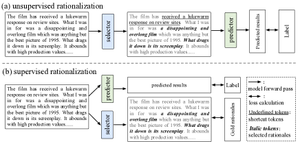
Figure 1: Schematic of rationalization methods presented in this paper. (a) is the process of unsupervised rationalization with the selector-predictor pattern. (b) illustrates the supervised rationalization with a multi-task framework. Semi-rationalization can be considered the combination of (a) and (b).

Among them, the underlined tokens extracted by the unsupervised rationalization method are the shortcut tokens, where a poor quality movie is always associated with “received a lukewarm response”. An unsupervised rationalization is easy to predict the movie as “negative” based on these shortcut tokens. However, for a human being, judging a movie is not influenced by other movie reviews (i.e., even if a movie has a low rating on movie review sites, someone will still enjoy it). Therefore, although the model predicts the right outcome, it still fails to reveal true rationales for predicting labels but depending on the shortcuts. In general, while shortcuts are potentially effective in predicting task results, they are still damaging to compose rationales. Based on this conclusion, we can get an important assumption:

Assumption 1

A well-trained unsupervised rationalization model inevitably composes rationales with both the gold rationale and shortcuts tokens.

Then, as the second type is to include the gold rationales annotated by human during training (DeYoung et al., 2020; Li et al., 2022a; Chan et al., 2022), we denote it as “supervised rationalization”. It models the rationalization with a multi-task learning, optimizing the joint likelihood of class labels and extractive rationales (Figure 1(b)). Among them, the rationale prediction task can be considered as a token classification. Since this method exploits real rationales, the problem of adopting the shortcuts to predict task results can be mitigated. However, such extensive annotated rationales are infeasible to obtain for most tasks, rendering this method unavailable.

To combine the superiority of the above two types of methods, Pruthi et al. (2020); Bhat et al. (2021) propose a “semi-supervised rationalization” method, consisting of a two-phases training. They first train the rationalization task with few labeled rationales in a multi-task learning framework (the supervised phase) like the second type method, where we denote the used training dataset as $\mathcal{D}_{sup}$. Then, they train the remaining data $\mathcal{D}_{un}$ following the first type method (the unsupervised phase). Since this method still suffers from limited gold rationales and employing shortcuts to generate rationales, we argue this “semi-supervised pattern” can be further explored to improve the rationalization.

Along this research line, in this paper, we propose a boosted method Shortcuts-fused Selective Rationalization (SSR) which enhances the semi-supervised rationalization by exploring shortcuts. Different from the previous methods that are degraded by shortcuts, SSR explicitly exploits shortcuts in the data to yield more accurate task results and extract more plausible rationales. Specifically, in the semi-supervised setting, we first train SSR with $\mathcal{D}_{sup}$ in the supervised phase. Among them, since there exist no labeled shortcuts, we design a shortcuts discovery approach to identify several potential shortcut tokens in $\mathcal{D}_{sup}$. In detail, we employ a trained unsupervised rationalization model to infer potential rationales in $\mathcal{D}_{sup}$. As discussed in Assumption 1, the rationales extracted by unsupervised rationalization inevitably contain several shortcut tokens. Then, by introducing the gold rationales, we can explicitly obtain the shortcut tokens. Next, we design two strategies to learn the extracted shortcut information and further transfer it into the unsupervised phase, which can mitigate the problem of adopting shortcuts to yield rationales. Besides, due to the limited rationales labels, we develop two data augmentations methods, including a random data augmentation and semantic augmentation, by replacing identified shortcut tokens in $\mathcal{D}_{sup}$. To validate the effectiveness of our proposed SSR, we conduct extensive experiments on five datasets from the ERASER benchmark (DeYoung et al., 2020). The experimental results empirically show that SSR consistently outperforms the competitive unsupervised and semi-supervised baselines on both the task prediction and rationale generation by a significant margin, and achieves comparable results to supervised baselines.

2 Problem Formulation

Considering a text classification task, given the text input $x=\left\{x_{1},x_{2},\ldots,x_{n}\right\}$ and the ground truth $y$, where $x_{i}$ represents the $i$-th token, the goal is employing a predictor to yield the prediction results ${y}$ while learning a mask variable $m=\left\{m_{1},m_{2},\ldots,m_{n}\right\}$ by a selector. Among them, $m_{j}\in\{0,1\}$ indicates whether the $i$-th token is a part of the rationale. Then, the selected rationale is defined as $z=m\odot x=\left\{m_{1}\cdot x_{1},m_{2}\cdot x_{2},\ldots,m_{n}\cdot x_{n}\right\}$. Take the case in Figure 1 for example, the selective rationalization aims to yield an accurate prediction result (i.e., negative) and extract the rationale (the italic tokens) as the supporting evidence to explain this result.

3 Preliminary of Selective Rationalization

Unsupervised rationalization. In the unsupervised rationalization, since the gold rationales are unavailable, to achieve extracting rationales, this type of method trains the selector and predictor in tandem. Specifically, the selector first maps each token $x_{i}$ to its probability, $p_{\theta}(\widetilde{m}_{i}|x_{i})$ of being selected as part of rationale, where $p_{\theta}(\widetilde{m}_{i}|x_{i})=\textrm{softmax}(W_{s_{un}}f_{s_{un}}(x_{i}))$. Among them, $f_{s_{un}}(\cdot)$ represents an encoder (e.g. BERT (Devlin et al., )), encoding $x_{i}$ into a $d$-dimensional vector, and ${W}_{s_{un}}\in\mathbb{R}^{2\times d}$. Then, to sample $m_{i}\in\{0,1\}$ from the $p_{\theta}(\widetilde{m}_{i}|x_{i})$ distribution and ensure this operation differentiable, Lei et al. (2016) introduce a Bernoulli distribution with REINFORCE (Williams, 1992). Since this method may be quite unstable (Paranjape et al., 2020), in this paper, we implement this sampling operation with a Gumbel-Softmax reparameterization (Jang et al., 2017):

$$m_{i}=\frac{\exp\left(\left(\log\left(p_{\theta}(\widetilde{m}_{i}|x_{i})\right)+g_{i}\right)/\tau\right)}{\sum_{j}\exp\left(\left(\log\left(p_{\theta}(\widetilde{m}_{j}|x_{j})\right)+g_{j}\right)/\tau\right)},$$ (1)

where $g_{i}=-\log\left(-\log\left(u_{i}\right)\right)$ and $\tau$ is a temperature hyperparameter. $u_{i}$ is sampled from a uniform distribution $U(0,1)$. Details of Gumbel-Softmax are shown in Appendix C.1. Naturally, the rationale $z$ extracted by the selector is calculated as $z=m\odot x$.

Next, the predictor $q_{\psi}(y|z)$ yields the prediction results solely based on the rationale $z$, where $q_{\psi}(y|z)=\textrm{softmax}(W_{p_{un}}f_{p_{un}}(z))$. Wherein $f_{p_{un}}(\cdot)$ re-encodes $z$ into $d$-dimensional continuous hidden states, $W_{p_{un}}\in\mathbb{R}^{N\times d}$ is the learned parameters, and $N$ is the number of labels (e.g., $N=2$ in the binary classification). Finally, the prediction loss can be formulated as :

$$\mathcal{L}_{un\_task}=\mathbb{E}_{\begin{subarray}{c}{x},y\sim\mathcal{D}_{un}\\ {m}\sim p_{\theta}({\widetilde{m}}|x)\end{subarray}}\left[-\log q_{\psi}(y|m\odot x)\right],$$ (2)

where $\mathcal{D}_{un}$ is a training set (gold rationales are unavailable). Besides, to impose the selected rationales are short and coherent, we incorporate sparsity and continuity constraints into the rationalization:

$$\mathcal{L}_{re}=\underbrace{\lambda_{1}\left|\frac{1}{n}\sum_{i=1}^{n}m_{i}-\alpha\right|}_{sparsity}+\underbrace{\lambda_{2}\sum_{i=2}^{n}\left|{m}_{i}-{m}_{i-1}\right|}_{continuity},$$ (3)

where $\alpha\in[0,1]$ is the predefined sparsity level (the higher the $\alpha$, the lower the sparsity). Finally, the objective of the unsupervised rationalization is defined as $\mathcal{L}_{un}=\mathcal{L}_{un\_task}+\mathbb{E}_{\begin{subarray}{c}{m}\sim p_{\theta}({\widetilde{m}}|x)\end{subarray}}\left[\mathcal{L}_{re}\right]$.

Although this type of method can extract rationales without the labeled rationales supervision and achieve promising results (Bastings et al., 2019; Sha et al., 2021; Yu et al., 2021), Chang et al. (2020); Wu et al. (2022) have proved that it is prone to exploiting the shortcuts in data (e.g., the statistics shortcuts) to yield prediction results and rationales. In other words, such shortcut-involved rationales fail to reveal the underlying relationship between inputs and rationales.

Supervised rationalization. Since both the ground truth and the human annotated rationales are available in supervised rationalization, several researches (Li et al., 2022a; Chan et al., 2022) introduce a joint task classification and rationalization method. Specifically, in the supervised rationalization, we denote $\mathcal{D}_{sup}$ as a joint task and rationale labeled training set, containing additional annotated rationales $\hat{z}$. Then, similar to the unsupervised rationalization, we generate the probability of selecting $x_{i}$ as the part of rationales by calculating $p_{\theta}(\widetilde{m}_{i}|x_{i})=\textrm{softmax}(W_{s_{sup}}f_{s_{sup}}(x_{i}))$. Next, given gold rationales $\hat{z}$, we can consider the rationalization task as a binary token classification, and calculate the corresponding loss with token-level binary cross-entropy (BCE) criterion :

$$\mathcal{L}_{select}=\sum_{i=1}^{n}-\hat{m}_{i}\log p_{\theta}(\widetilde{m}_{i}|x_{i}),$$ (4)

where $\hat{m}=\left\{\hat{m}_{1},\hat{m}_{2},\ldots,\hat{m}_{n}\right\}$ is the gold mask corresponding to $\hat{z}$. Next, for the task classification, different from the unsupervised rationalization employing extracted rationales as the input, the predictor in supervised rationalization yields results with $q_{\psi}(y|x)$, and the prediction loss is calculated as $\mathcal{L}_{sup\_task}=\mathbb{E}_{\begin{subarray}{c}{x},y\sim\mathcal{D}_{sup}\end{subarray}}\left[-\log q_{\psi}(y|x)\right]$, where $q_{\psi}(y|x)=\textrm{softmax}(W_{p_{sup}}f_{p_{sup}}(x))$. Finally, the objective of supervised rationalization is $\mathcal{L}_{sup}=\mathcal{L}_{sup\_task}+\mathbb{E}_{\begin{subarray}{c}{x},z\sim\mathcal{D}_{sup}\end{subarray}}\left[\mathcal{L}_{select}\right]$.

Since the real rationale label is explicitly introduced into the supervised rationalization, the “shortcuts” problem posed by unsupervised methods can be eased. However, such extensive rationales annotated by human are the main bottleneck enabling the widespread application of these models.

Semi-supervised rationalization. For the semi-supervised rationalization, researchers (Paranjape et al., 2020; Pruthi et al., 2020; Bhat et al., 2021) consider a low-resource setup where they have annotated rationales for part of the training data $\mathcal{D}_{semi}$. In other words, $\mathcal{D}_{semi}$ consists of $\mathcal{D}_{un}$ and $\mathcal{D}_{sup}$, where $|\mathcal{D}_{un}|\gg|\mathcal{D}_{sup}|$. Then, we use the following semi-supervised objective: $\mathcal{L}_{semi}=\mathcal{L}_{sup}+\mathcal{L}_{un}$, where we first train the model on $\mathcal{D}_{sup}$ and then on $\mathcal{D}_{un}$.

Despite this method appearing to combine the advantages of the previous two methods, it is still prone to adopting shortcuts for prediction ($\mathcal{L}_{un}$ in $\mathcal{L}_{semi}$). Besides, due to the gap in data size between the two datasets (i.e., $\mathcal{D}_{un}$ and $\mathcal{D}_{sup}$), the prediction performance of this semi-supervised approach is considerably degraded compared to the supervised rationalization (Bhat et al., 2021).

4 Shortcuts-fused Selective Rationalization

In this section, we follow the above semi-supervised rationalization framework and further propose a Shortcuts-fused Selective Rationalization (SSR) method by discovering shortcuts in data. We first identify shortcut tokens from the input by exploring gold rationales in $\mathcal{D}_{sup}$ (section 4.1). Then, to mitigate the problem which exploits shortcuts for prediction, we introduce two strategies by leveraging identified shortcuts (section 4.2). Finally, to bridge the data size gap between $\mathcal{D}_{un}$ and $\mathcal{D}_{sup}$, we develop two data augmentation methods also depending on identified shortcuts (section 4.3).

4.1 Shortcuts Discovery

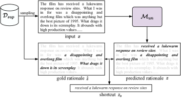
Figure 2: Process of the shortcut generator.

As described above, identifying and detecting shortcuts in the data is fundamental to our approach. However, since there exist no labeled shortcuts, posing a challenge to discover shortcuts. Based on Assumption 1, we can identify the potential shortcut token from rationales extracted by a well-trained unsupervised rationalization model via introducing labeled rationale tokens.

Definition 1 (Potential Shortcut Token) We first assume the unsupervised rationalization model $\mathcal{M}_{un}$ is already trained. Then, given the annotated rationales $\hat{z}$ and rationales $z$ extracted by $\mathcal{M}_{un}$, we define $\mathbb{PST}(x_{i})$ as whether a token $x_{i}$ is considered to be a potential shortcut token or not:

$$\mathbb{PST}(x_{i})=\mathbb{I}(x_{i}\in{z}\wedge x_{i}\notin\hat{z}),$$ (5)

where $\wedge$ is the logical operation AND. $\mathbb{PST}(x_{i})$$=$$1$ denotes $x_{i}$ is defined as a potential shortcut token.

Motivated by the above assumption and definition, our shortcuts discovery method is two-fold:

(i) We train an unsupervised rationalization method $\mathcal{M}_{un}$ with $\mathcal{D}_{un}$, which sufficiently exploits shortcuts to make predictions.

(ii) We design a shortcut generator (Figure 2) to combine labeled rationales in $\mathcal{D}_{sup}$ and $\mathcal{M}_{un}$ to identify shortcuts. Specifically, the shortcut generator first employs $\mathcal{M}_{un}$ to infer the potential rationales $z$ in $\mathcal{D}_{sup}$. Next, we introduce the gold rationales $\hat{z}$ and compare them with the predicted rationales $z$. If a token $x_{i}\in{z}$ and $x_{i}\notin\hat{z}$ (i.e., this token is incorrectly predicted as rationale tokens), we define it as a potential shortcut token.

Figure 3: Architecture of $\textmd{SSR}_{virt}$ consisting of the supervised and unsupervised phases. Among them, represents the frozen shortcut imitator, and white boxes in $m$ indicate the rationale tokens and the black are non-rationale ones.

In the practical implementation, considering the coherence of rationales, we identify a subsequence with three or more consecutive potential shortcut tokens as the shortcut $z_{s}$. For example, as shown in Figure 2, $\mathcal{M}_{un}$ has predicted the movie review as “negative” correctly and composed the predicted rationales. By comparing with gold rationales, we identify “received a lukewarm response on review sites” as shortcuts. It’s worth noting that the shortcut discovery is only used in the training phase.

4.2 Two Strategies by Exploring Shortcuts

As mentioned previously, we follow the semi-rationalization framework and train SSR on $\mathcal{D}_{un}$ and $\mathcal{D}_{sup}$ in tandem. Since we have identified the shortcuts in $\mathcal{D}_{sup}$, we design two strategies by exploring identified shortcuts to mitigate the impact of adopting shortcuts for prediction in $\mathcal{D}_{un}$.

4.2.1 Shared Parameters.

Before we introduce the two strategies, we present the shared parameters in both unsupervised and supervised rationalization. Here, we let “$A\leftrightarrow B$” represent the parameter $A$ and $B$ share parameters.

$\bullet$ To allow the model to capture richer interactions between task prediction and rationales selection, we adopt $f_{s_{un}}(\cdot)\leftrightarrow f_{p_{un}}(\cdot)$, and $f_{s_{sup}}(\cdot)\leftrightarrow f_{p_{sup}}(\cdot)$ (Bhat et al., 2021; Liu et al., 2022).

$\bullet$ To let the unsupervised and supervised rationalization learn better from each other, we let $W_{s_{un}}f_{s_{un}}(\cdot)\leftrightarrow W_{s_{sup}}f_{s_{sup}}(\cdot)$ in the selector. $W_{p_{un}}f_{p_{un}}(\cdot)\leftrightarrow W_{p_{sup}}f_{p_{sup}}(\cdot)$ in the predictor.

In summary, all encoders in both selector and predictor share parameters: $f_{s_{un}}(\cdot)\leftrightarrow f_{p_{un}}(\cdot)\leftrightarrow f_{s_{sup}}(\cdot)\leftrightarrow f_{p_{sup}}(\cdot)$. Linear parameters in selector are shared: $W_{s_{un}}\leftrightarrow W_{s_{sup}}$. Linear parameters in predictor are shared: $W_{p_{un}}\leftrightarrow W_{p_{sup}}$. For clarity, in both unsupervised and supervised rationalization, we represent the $f_{s}(\cdot)$ and $f_{p}(\cdot)$ as the encoder in selector and predictor, $W_{s}$ and $W_{p}$ are the corresponding linear parameters. Table LABEL:share-p in Appendix C.2 lists all shared parameters.

4.2.2 Injecting Shortcuts into Prediction.

In the semi rationalization, the unsupervised rationalization may still identify the shortcuts as rationales due to the unavoidable limitations (section 3). To this end, we propose a strategy, injecting shortcuts into the task prediction. Specifically:

In the supervised phase, besides the original loss $\mathcal{L}_{sup}$, we add a “uniform” constraint to ensure the predictor $q_{\psi}$ identifies the shortcuts features as meaningless features:

$$\mathcal{L}_{unif}=\mathbb{E}_{\begin{subarray}{c}z_{s}\sim\mathcal{D}_{sup}\end{subarray}}\left[\operatorname{KL}\left(\mathcal{U}(0,|N|)\|q_{\psi}(y|z_{s})\right)\right],$$ (6)

where KL denotes the Kullback–Leibler divergence, $|N|$ is the total number of classes, and $\mathcal{U}(0,|N|)$ denotes the uniform class distribution. When the predictor $q_{\psi}(y|x)$ adopts the input to yield task results, Eq (6) encourages the predictor to identify shortcut tokens $z_{s}$ as meaningless tokens, and disentangles shortcuts features from the input ones (i.e., making shortcuts and rationales de-correlated).

In the unsupervised phase, the learned features information can be transferred into the unsupervised rationalization method through the shared predictor ($W_{p_{un}}f_{p_{un}}(\cdot)\leftrightarrow W_{p_{sup}}f_{p_{sup}}(\cdot)$).

Finally, we denote SSR with this strategy as $\textmd{SSR}_{unif}$, and the objective of $\textmd{SSR}_{unif}$ can be defined as the sum of the losses: $\mathcal{L}_{ssr_{unif}}=\mathcal{L}_{un}+\mathcal{L}_{sup}+\lambda_{unif}\mathcal{L}_{unif}$. Detailed algorithms of $\textmd{SSR}_{unif}$ are shown in Appendix A.1.

Table 1: Task F1 and Token F1 of selected rationales for the five datasets. Among them, the underlined scores are the state-of-the-art performances of the supervised rationalization. The results in bold are the best scores in our SSR and its variants.

Methods	Movies		MultiRC		BoolQ		Evidence Inference		FEVER
	Task	Token-F1	Task	Token-F1	Task	Token-F1	Task	Token-F1	Task	Token-F1
Vanilla Un-RAT	87.0 $\pm$ 0.1	28.1 $\pm$ 0.2	57.7 $\pm$ 0.4	23.9 $\pm$ 0.5	62.0 $\pm$ 0.2	19.7 $\pm$ 0.4	46.2 $\pm$ 0.5	8.9 $\pm$ 0.2	71.3 $\pm$ 0.4	25.4 $\pm$ 0.7
IB	84.0 $\pm$ 0.0	27.5 $\pm$ 0.0	62.1 $\pm$ 0.0	24.9 $\pm$ 0.0	65.2 $\pm$ 0.0	12.8 $\pm$ 0.0	46.3 $\pm$ 0.0	6.9 $\pm$ 0.0	84.7 $\pm$ 0.0	42.7 $\pm$ 0.0
INVRAT	87.7 $\pm$ 1.2	28.6 $\pm$ 0.9	61.8 $\pm$ 1.0	30.4 $\pm$ 1.5	64.9 $\pm$ 2.5	20.8 $\pm$ 1.1	47.0 $\pm$ 1.8	9.0 $\pm$ 1.5	83.6 $\pm$ 1.8	41.4 $\pm$ 1.4
Inter-RAT	88.0 $\pm$ 0.7	28.9 $\pm$ 0.4	62.2 $\pm$ 0.7	30.7 $\pm$ 0.5	65.8 $\pm$ 0.4	21.0 $\pm$ 0.4	46.4 $\pm$ 0.6	9.9 $\pm$ 0.4	85.1 $\pm$ 0.5	43.0 $\pm$ 0.8
MCD	89.1 $\pm$ 0.3	29.1 $\pm$ 0.5	62.8 $\pm$ 0.4	31.1 $\pm$ 0.6	65.2 $\pm$ 0.4	23.1 $\pm$ 0.8	47.1 $\pm$ 0.6	10.8 $\pm$ 0.7	84.4 $\pm$ 0.6	44.6 $\pm$ 0.2
Vanilla Semi-RAT	89.8 $\pm$ 0.2	30.4 $\pm$ 0.2	63.3 $\pm$ 0.4	55.4 $\pm$ 0.2	57.3 $\pm$ 0.3	43.0 $\pm$ 0.1	46.1 $\pm$ 0.5	25.1 $\pm$ 0.2	82.6 $\pm$ 0.6	40.7 $\pm$ 0.8
IB (25% rationales)	85.4 $\pm$ 0.0	28.2 $\pm$ 0.0	66.4 $\pm$ 0.0	54.0 $\pm$ 0.0	63.4 $\pm$ 0.0	19.2 $\pm$ 0.0	46.7 $\pm$ 0.0	10.8 $\pm$ 0.0	88.8 $\pm$ 0.0	63.9 $\pm$ 0.0
WSEE	90.1 $\pm$ 0.1	32.2 $\pm$ 0.1	65.0 $\pm$ 0.8	55.8 $\pm$ 0.5	59.9 $\pm$ 0.4	43.6 $\pm$ 0.4	49.2 $\pm$ 0.9	14.8 $\pm$ 0.8	84.3 $\pm$ 0.3	44.9 $\pm$ 0.5
ST-RAT	87.0 $\pm$ 0.0	31.0 $\pm$ 0.0	-	-	62.0 $\pm$ 0.0	51.0 $\pm$ 0.0	46.0 $\pm$ 0.0	9.0 $\pm$ 0.0	89.0 $\pm$ 0.0	39.0 $\pm$ 0.0
Vanilla Sup-RAT	93.6 $\pm$ 0.3	38.2 $\pm$ 0.2	63.8 $\pm$ 0.2	59.4 $\pm$ 0.4	61.5 $\pm$ 0.3	51.3 $\pm$ 0.2	52.3 $\pm$ 0.5	16.5 $\pm$ 0.2	83.6 $\pm$ 1.4	68.9 $\pm$ 0.9
Pipeline	86.0 $\pm$ 0.0	16.2 $\pm$ 0.0	63.3 $\pm$ 0.0	41.2 $\pm$ 0.0	62.3 $\pm$ 0.0	18.4 $\pm$ 0.0	70.8 $\pm$ 0.0	54.8 $\pm$ 0.0	87.7 $\pm$ 0.0	81.2 $\pm$ 0.0
UNIREX	91.3 $\pm$ 0.4	39.8 $\pm$ 0.6	65.5 $\pm$ 0.8	62.1 $\pm$ 0.2	61.9 $\pm$ 0.7	51.4 $\pm$ 0.6	48.8 $\pm$ 0.3	21.3 $\pm$ 0.1	81.1 $\pm$ 0.8	70.9 $\pm$ 0.5
AT-BMC	92.9 $\pm$ 0.6	40.2 $\pm$ 0.3	65.8 $\pm$ 0.2	61.1 $\pm$ 0.5	62.1 $\pm$ 0.2	52.1 $\pm$ 0.2	49.5 $\pm$ 0.4	18.6 $\pm$ 0.3	82.3 $\pm$ 0.3	71.1 $\pm$ 0.6
$\textmd{SSR}_{unif}$	94.3 $\pm$ 0.3	33.2 $\pm$ 0.4	62.8 $\pm$ 0.3	56.2 $\pm$ 0.2	60.8 $\pm$ 0.4	47.6 $\pm$ 0.5	46.8 $\pm$ 0.3	26.8 $\pm$ 0.2	86.8 $\pm$ 0.9	46.6 $\pm$ 0.2
+random DA	90.7 $\pm$ 0.3	34.5 $\pm$ 0.1	63.6 $\pm$ 0.5	56.1 $\pm$ 0.3	61.3 $\pm$ 0.7	48.3 $\pm$ 0.5	46.0 $\pm$ 0.1	33.1 $\pm$ 0.2	87.4 $\pm$ 0.3	47.6 $\pm$ 0.5
+semantic DA	90.7 $\pm$ 0.2	35.6 $\pm$ 0.2	64.7 $\pm$ 0.7	42.7 $\pm$ 0.4	58.0 $\pm$ 0.3	50.2 $\pm$ 0.3	48.7 $\pm$ 0.2	33.5 $\pm$ 0.4	87.9 $\pm$ 0.6	48.0 $\pm$ 0.8
+mixed DA	94.5 $\pm$ 0.2	35.1 $\pm$ 0.1	65.3 $\pm$ 0.6	40.3 $\pm$ 0.5	60.4 $\pm$ 0.2	49.2 $\pm$ 0.5	47.6 $\pm$ 0.1	35.2 $\pm$ 0.2	88.3 $\pm$ 0.3	48.8 $\pm$ 0.7
$-$shared $W_{s}$ and $W_{p}$	88.3 $\pm$ 0.1	29.8 $\pm$ 0.6	60.2 $\pm$ 0.3	55.7 $\pm$ 0.5	57.4 $\pm$ 0.3	43.5 $\pm$ 0.2	45.6 $\pm$ 0.3	24.9 $\pm$ 0.2	81.4 $\pm$ 0.3	39.3 $\pm$ 0.7
$\textmd{SSR}_{virt}$	90.0 $\pm$ 0.0	34.6 $\pm$ 0.2	64.2 $\pm$ 0.3	57.0 $\pm$ 0.2	58.2 $\pm$ 0.5	43.8 $\pm$ 0.3	50.4 $\pm$ 0.3	31.3 $\pm$ 0.4	87.1 $\pm$ 0.4	47.0 $\pm$ 0.5
+random DA	92.8 $\pm$ 0.2	36.7 $\pm$ 0.2	65.4 $\pm$ 0.2	44.3 $\pm$ 0.4	58.3 $\pm$ 0.6	47.7 $\pm$ 0.3	46.5 $\pm$ 0.3	32.4 $\pm$ 0.2	87.4 $\pm$ 0.3	47.5 $\pm$ 0.9
+semantic DA	87.6 $\pm$ 0.3	36.9 $\pm$ 0.1	66.2 $\pm$ 0.5	49.8 $\pm$ 0.4	61.1 $\pm$ 0.3	48.8 $\pm$ 0.2	46.5 $\pm$ 0.4	31.1 $\pm$ 0.2	88.9 $\pm$ 0.2	49.0 $\pm$ 0.1
+mixed DA	90.5 $\pm$ 0.2	37.4 $\pm$ 0.1	64.5 $\pm$ 0.6	53.1 $\pm$ 0.4	60.3 $\pm$ 0.2	49.1 $\pm$ 0.1	47.1 $\pm$ 0.4	33.4 $\pm$ 0.3	88.0 $\pm$ 0.4	48.5 $\pm$ 0.6
$-$shared $W_{s}$ and $W_{p}$	87.9 $\pm$ 0.5	31.9 $\pm$ 0.4	62.6 $\pm$ 0.3	55.3 $\pm$ 0.2	57.6 $\pm$ 0.4	43.3 $\pm$ 0.5	48.6 $\pm$ 0.2	25.8 $\pm$ 0.4	82.3 $\pm$ 0.5	40.3 $\pm$ 0.6
$-$shared $W_{a}$ and $W_{p}$	88.3 $\pm$ 0.3	30.4 $\pm$ 0.1	62.4 $\pm$ 0.9	54.0 $\pm$ 2.1	57.5 $\pm$ 0.3	42.9 $\pm$ 0.1	45.8 $\pm$ 0.4	25.0 $\pm$ 0.2	81.8 $\pm$ 0.7	39.6 $\pm$ 0.7

4.2.3 Virtual Shortcuts Representations.

Intuitively, the supervised rationalization with gold rationales will perform better than the semi-supervised one. However, due to the limited resource, it is difficult for us to annotate the rationales with $\mathcal{D}_{un}$ and further obtain shortcut tokens to improve the performance. To close the resource gap, we propose a virtual shortcuts representations strategy ($\textmd{SSR}_{virt}$) with transferred shortcuts knowledge from $\mathcal{D}_{sup}$ as guidance. As shown in Figure 3, $\textmd{SSR}_{virt}$ also contains two phases (the supervised and unsupervised phase). Specifically:

In the supervised phase, when training the supervised rationalization with $\mathcal{D}_{sup}$, we first adopt an external predictor $q_{\eta}(y|z_{s})$ to predict task results based on the shortcuts $z_{s}$, and ensure the encoder $f_{p_{\eta}}(\cdot)$ in $q_{\eta}$ captures sufficient shortcuts representations $f_{p_{\eta}}(z_{s})\in\mathbb{R}^{d}$ by minimizing :

$$\mathcal{L}_{s}=\mathbb{E}_{\begin{subarray}{c}z_{s}\sim\mathcal{D}_{sup}\end{subarray}}\left[-\log q_{\eta}(y|z_{s})\right]=\mathbb{E}_{\begin{subarray}{c}z_{s}\sim\mathcal{D}_{sup}\end{subarray}}\left[-\log\textrm{softmax}(W_{\eta}f_{p_{\eta}}(z_{s}))\right].\vspace{-0.2cm}$$ (7)

Then, we learn an additional shortcut imitator $f_{a}(x_{sup})$ that takes $x$ in $\mathcal{D}_{sup}$ as the input (denoted by $x_{sup}$ for clarity) to align and mimic $f_{p_{\eta}}(z_{s})$ by minimizing the squared euclidean distance of these two representations, where $f_{a}(\cdot)$ and $f_{p_{\eta}}(\cdot)$ share parameters:

$$\mathcal{L}_{virt}=\mathbb{E}_{\begin{subarray}{c}x_{sup},z_{s}\sim\mathcal{D}_{sup}\end{subarray}}\left[\left\|f_{p_{\eta}}(z_{s})-f_{a}(x_{sup})\right\|^{2}\right].$$ (8)

In the unsupervised phase, during training with $\mathcal{D}_{un}$, we keep $f_{a}(\cdot)$ frozen and employ it to generate virtual shortcuts representations $f_{a}(x_{un})$ by taking $x$ in $\mathcal{D}_{un}$ as the input. After that, to encourage the model to remove the effect of shortcuts on task predictions, we first adopt $f_{a}(x_{un})$ to match a uniform distribution by calculating

$$\mathcal{L}_{diff}=\mathbb{E}_{\begin{subarray}{c}x\sim\mathcal{D}_{un}\end{subarray}}\left[\operatorname{KL}\left(\mathcal{U}(0,|N|)\|q_{\sigma}(y|x_{un})\right)\right],$$ (9)

where $q_{\sigma}(y|x_{un})=\textrm{softmax}(W_{a}f_{a}(x_{un}))$. Next, we set $W_{a}$ and $W_{p}$ share parameters (i.e., $W_{a}\leftrightarrow W_{p}$) to transfer the shortcut information into the predictor $f_{p}$, and further achieve the de-correlation of shortcuts and rationales. Formally, the final objective of $\textmd{SSR}_{virt}$ is $\mathcal{L}_{{ssr}_{virt}}=\mathcal{L}_{un}+\mathcal{L}_{sup}+\mathcal{L}_{s}+\lambda_{virt}\mathcal{L}_{virt}+\lambda_{diff}\mathcal{L}_{diff}$. Detailed algorithms of $\textmd{SSR}_{virt}$ are shown in Appendix A.2.

4.3 Data Augmentation

In this section, to close the quantitative gap between $\mathcal{D}_{un}$ and $\mathcal{D}_{sup}$, we propose two data augmentation (DA) methods by utilizing identified shortcuts in $\mathcal{D}_{sup}$.

Random Data Augmentation. As we have identified the potential shortcuts $z_{s}$ in $\mathcal{D}_{sup}$, we can replace these shortcuts tokens with other tokens which are sampled randomly from the datastore $\mathbb{D}_{random}$. Among them, the database $\mathbb{D}_{random}$ contains all tokens of $\mathcal{D}_{un}$ and $\mathcal{D}_{sup}$ (i.e., $\mathbb{D}_{random}=\left\{x_{j},\forall x_{j}\in\mathcal{D}_{un}\vee x_{j}\in\mathcal{D}_{sup}\right\}$).

Table 2: Task F1 and Token F1 of selected rationales for the five datasets with random DA.

Methods	Movies		MultiRC		BoolQ		Evidence Inference
+ random DA	Task	Token-F1	Task	Token-F1	Task	Token-F1	Task	Token-F1
Vanilla Un-RAT	88.0 $\pm$ 0.4	28.4 $\pm$ 0.3	58.4 $\pm$ 0.2	24.7 $\pm$ 0.3	62.1 $\pm$ 0.3	23.5 $\pm$ 0.2	47.0 $\pm$ 0.4	10.4 $\pm$ 0.3
Vanilla Semi-RAT	90.6 $\pm$ 0.3	31.6 $\pm$ 0.1	64.2 $\pm$ 0.4	56.2 $\pm$ 0.3	58.9 $\pm$ 0.1	44.5 $\pm$ 0.3	45.0 $\pm$ 0.3	26.0 $\pm$ 0.3
WSEE	89.9 $\pm$ 0.4	33.4 $\pm$ 0.3	65.3 $\pm$ 0.1	55.7 $\pm$ 0.3	61.0 $\pm$ 0.2	45.5 $\pm$ 0.3	50.0 $\pm$ 0.3	18.7 $\pm$ 0.5
Vanilla Sup-RAT	93.0 $\pm$ 0.4	39.1 $\pm$ 0.3	64.4 $\pm$ 0.6	60.6 $\pm$ 0.2	62.1 $\pm$ 0.4	51.9 $\pm$ 0.7	52.8 $\pm$ 0.2	18.5 $\pm$ 0.3
AT-BMC	92.8 $\pm$ 0.1	40.4 $\pm$ 0.3	66.6 $\pm$ 0.6	61.8 $\pm$ 0.5	62.0 $\pm$ 0.1	52.6 $\pm$ 0.2	49.5 $\pm$ 0.3	19.4 $\pm$ 0.6
$\textmd{SSR}_{unif}$	90.7 $\pm$ 0.3	34.5 $\pm$ 0.1	63.6 $\pm$ 0.5	56.1 $\pm$ 0.3	61.3 $\pm$ 0.7	48.3 $\pm$ 0.5	46.0 $\pm$ 0.1	33.1 $\pm$ 0.2
$\textmd{SSR}_{virt}$	92.8 $\pm$ 0.2	36.7 $\pm$ 0.2	65.4 $\pm$ 0.2	44.3 $\pm$ 0.4	58.3 $\pm$ 0.6	47.7 $\pm$ 0.3	46.5 $\pm$ 0.3	32.4 $\pm$ 0.2

Semantic Data Augmentation. Besides the random augmentation, we design a retrieval-grounded semantic augmentation method by replacing shortcut tokens with several tokens semantically close to them through retrieval. Detailed retrieval algorithms about semantic DA are shown in Appendix A.3. Besides, we also mix data augmented from random DA with data augmented from semantic DA to achieve mixed data augmentation.

5 Experiments

5.1 Datasets and Comparison Methods

Datasets. We evaluate SSR on text classification tasks from the ERASER benchmark (DeYoung et al., 2020), including Movies (Pang & Lee, 2004) for sentiment analysis, MultiRC (Khashabi et al., 2018) for multiple-choice QA, BoolQ (Clark et al., 2019) for reading comprehension, Evidence Inference (Lehman et al., 2019) for medical interventions, and FEVER (Thorne et al., 2018) for fact verification. Each dataset contains human annotated rationales and classification labels. In the semi-supervised (or unsupervised) setting, partially (or fully) labeled rationales are unavailable.

Comparison Methods. We compare SSR against three type methods as follows:

$\bullet$ Unsupervised rationalization: Vanilla Un-RAT is the method presented in section 3, which samples rationale tokens from a Bernoulli distribution of each token with a Gumbel-softmax reparameterization. In practice, we employ Vanilla Un-RAT as the unsupervised rationalization method $\mathcal{M}_{un}$ in section 2. IB (Paranjape et al., 2020) employs an Information Bottleneck (Alemi et al., 2017) principle to manage the trade-off between achieving accurate classification performance and yielding short rationales. INVRAT (Chang et al., 2020) learns invariant rationales by exploiting multiple environments to remove shortcuts in data. Inter-RAT (Yue et al., 2022b) proposes a causal intervention method to remove spurious correlations in selective rationalization. MCD (Liu et al., 2023) uncover the conditional independence relationship between the target label and non-causal and causal features to compose rationales.

$\bullet$ Supervised rationalization: Vanilla Sup-RAT is the method we describe in section 3, which trains task classification and rationalization jointly. Pipeline (Lehman et al., 2019) is a pipeline model which trains the selector with gold rationales and predictor with class labels independently. UNIREX (Chan et al., 2022) proposes a unified supervised rationalization framework to compose faithful and plausible rationales. AT-BMC (Li et al., 2022a) is the state-of-the-art (SOTA) supervised rationalization approach, which is implemented with label embedding and mixed adversarial training.

$\bullet$ Semi-supervised rationalization: Vanilla Semi-RAT is the method described in section 3, which can be seen as the ablation of SSR (i.e., without exploiting shortcuts). IB (25% rationales) (Paranjape et al., 2020) trains the selector with 25% annotated rationales through the BCE loss, and employs the rest data to train the unsupervised IB. WSEE (Pruthi et al., 2020) proposes a classify-then-extract framework, conditioning rationales extraction on the predicted label. ST-RAT (Bhat et al., 2021) presents a self-training framework by exploiting the pseudo-labeled rationale examples.

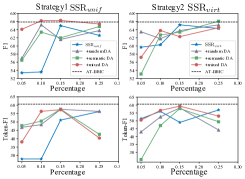
Figure 4: Gold Rationale Efficiency.

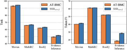
Figure 5: $\textmd{SSR}_{unif}$ with full annotations.

5.2 Experimental Setup

Following prior researches (Paranjape et al., 2020; Bhat et al., 2021), we employ BERT (Devlin et al., ) as the encoder in both the selector and predictor. For training, we adopt the AdamW optimizer (Loshchilov & Hutter, 2019) with an initial learning rate as 2e-05, then we set the batch size as 4, maximum sequence length as 512 and training epoch as 30. Besides, we set the predefined sparsity level $\alpha$ as $\{0.1,0.2,0.2,0.08\}$ for Movies, MultiRC, BoolQ and Evidence Inference, respectively, which is slightly higher than the percentage of rationales in the input text. In the semi-supervised setting, we implement our SSR and other semi-supervised rationalization methods with 25% labeled rationales. In SSR, we set $\mathcal{L}_{unif}$, $\mathcal{L}_{virt}$, and $\lambda_{diff}$ as 0.1, respectively. For evaluation, we report weighted F1 scores for classification accuracy following (Paranjape et al., 2020; Bhat et al., 2021).

Then, to evaluate quality of rationales, we report token-level F1 scores. For a fair comparison, results of IB, Pipeline and ST-RAT in Table 1 are directly taken (Paranjape et al., 2020; Bhat et al., 2021). Besides, as WSEE reports Macro F1 and AT-BMC reports Micro F1 for task classification, we re-run their released codes (Pruthi et al., 2020; Li et al., 2022a) and present weighted F1 scores.

5.3 Experimental Results

Overall Performance. We compare SSR with baselines across all the datasets, and experimental results are shown in Table 1. From the results, in general, we observe supervised rationalization methods perform the best, followed by semi-supervised rationalization, and unsupervised methods are the worst. Compared with the semi-supervised rationalization (e.g., ST-RAT), both $\textmd{SSR}_{unif}$ and $\textmd{SSR}_{virt}$ achieve promising performance, indicating the effectiveness of exploiting shortcuts to compose rationales. Besides, after data augmentations, our approach achieves a similar performance to the SOTA supervised rationalization method (i.e., AT-BMC). Considering that our method adopts only 25% annotated rationales, we argue that it is sufficient to demonstrate the strength of replacing the shortcut tokens for data augmentations. Finally, we compare $\textmd{SSR}_{unif}$ and $\textmd{SSR}_{virt}$. From the observation, we conclude $\textmd{SSR}_{virt}$ performs better than $\textmd{SSR}_{unif}$ in most datasets, illustrating employing virtual shortcuts representations to rationalization may be more effective with few labeled rationales.

Ablation study. For $\textmd{SSR}_{unif}$, we first let linear parameters $W_{s}$ and $W_{p}$ not share parameters and the results ($-$shared $W_{s}$ and $W_{p}$) are shown in the Table 1. We can find the results degrade significantly after removing the shared linear parameters. Then, we remove the uniform constraint. Since we implement Vanilla Sup-RAT with the same set of shared parameters, we argue that Vanilla Sup-RAT can be seen as the ablative variant of which removes the uniform constraint. From Table 1 in the paper, we find $\textmd{SSR}_{unif}$ outperforms Vanilla Sup-RAT. For $\textmd{SSR}_{virt}$, we set linear parameters $W_{s}$ and $W_{p}$ not share parameters, $W_{a}$ and $W_{p}$ not share parameters, respectively, and the results are shown in the Table 1. We also find the results degrade significantly after removing the shared linear parameters or the shared $W_{a}$ and $W_{p}$. Besides, the results of without the shared $W_{a}$ and $W_{p}$ perform worse than without shared linear parameters $W_{s}$ and $W_{p}$, indicating the effectiveness of the shared $W_{a}$ and $W_{p}$. From the observations, we can conclude that the components of $\textmd{SSR}_{unif}$ and $\textmd{SSR}_{virt}$ are necessary.

Analysis on Data Augmentation. We develop two data augmentation methods, including random DA and semantic DA. We augment the data with 25% of the original dataset for both random DA and semantic DA. From Table 1, we find SSR with semantic DA performs better than random DA, which validates that replacing shortcut tokens with semantically related tokens is more effective. Interestingly, SSR with mixed DA does not always perform better than semantic DA, and we argue a potential reason is that since the augmented data only replace part of the input tokens and most tokens in the text remain unchanged, the augmented data have many tokens that are duplicated from the original data, and too much of such data does not be beneficial for model training and even degrade it. Besides, we compare with baselines with the same data augmentation methods. Table 2 shows all baselines implemented with the random DA. With the same amount of data, our SSR achieves competitive results, especially in Token F1. More experimental results are shown in Appendix D.3.

Gold Rationale Efficiency. After the analysis on DA, we also find the performance of SSR with DA degrades a lot on the MultiRC dataset. Therefore, in this section, we investigate SSR performance with varying proportions of annotated rationales in the training set to see how much labeled data is beneficial for MultiRC. We make experiments on the MultiRC dataset and report corresponding results in Figure 5. From the figure, we observe both F1 and Token F1 of SSR increase with increasing proportions until 15%, and degrade when proportions exceed 15%. Meanwhile, the performance between $\textmd{SSR}_{unif}$+mixed DA with 15% gold rationales and AT-BMC is not significant. The above observation illustrates that more labeled rationales may be not better and SSR can effectively compose rationales and yield results without extensive manual rationales by exploring shortcuts. More experiments can be found in Appendix D.2.

SSR with Full Annotations. We investigate the performance of SSR with full annotations (i.e., the proportions of annotated rationales achieve 100%.). Specifically, for strategy 2, since there exist no shortcuts need to be “virtual”, $\textmd{SSR}_{virt}$ is unavailable. For strategy 1, $\textmd{SSR}_{unif}$ with full annotations means it has incorporated all identified shortcuts in the supervised phase. In Figure 5, we compare $\textmd{SSR}_{virt}$ with full annotations with AT-BMC that also exploits all labeled rationales. From the figure, we find $\textmd{SSR}_{virt}$ outperforms AT-BMC, indicating introducing all shortcuts into SSR is effective.

Besides, we also implement AT-BMC on Movies by introducing shortcuts (i.e., replace the original objective of AT-BMC $\mathcal{L}_{at-bmc}$ as $\mathcal{L}_{at-bmc}+\mathcal{L}_{unif}$ with Eq (6)). The corresponding F1 and Token F1 scores are 94.7 and 43.2, which still perform better than the original AT-BMC. Such observations strongly demonstrate that we can boost supervised rationalization by introducing shortcuts explicitly.

Table 3: Generalization Evaluation on IMDB and SST-2.

Methods	IMDB	SST-2
Vanilla Un-RAT	85.3 $\pm$ 0.2	45.3 $\pm$ 8.1
+semantic DA	86.6 $\pm$ 0.4	47.8 $\pm$ 6.6
Vanilla Semi-RAT	89.5 $\pm$ 0.4	75.9 $\pm$ 0.7
+semantic DA	89.7 $\pm$ 0.3	76.4 $\pm$ 0.5
WSEE	90.5 $\pm$ 0.3	77.1 $\pm$ 0.6
+semantic DA	91.0 $\pm$ 0.4	78.3 $\pm$ 0.7
$\textmd{SSR}_{unif}$	90.3 $\pm$ 0.2	79.4 $\pm$ 0.3
+semantic DA	90.7 $\pm$ 0.1	82.4 $\pm$ 0.8
$\textmd{SSR}_{virt}$	89.9 $\pm$ 0.2	79.9 $\pm$ 0.4
+semantic DA	90.3 $\pm$ 0.3	83.5 $\pm$ 0.5

Generalization Evaluation. Since SSR explicitly removes the effect of shortcuts on yielding task results and composing rationales, SSR can generalize better to out-of-distribution (OOD) datasets than unsupervised rationalization methods, where such unsupervised methods generalize poorly since the shortcuts are changed. To this end, we conduct an experiment to validate this opinion. Specifically, we introduce a new movie reviews dataset SST-2 (Socher et al., 2013) which contains pithy expert movie reviews. As the original Movies dataset in section 5.1 contains lay movie reviews (Hendrycks et al., 2020), SST-2 can be considered as the OOD dataset corresponding to Movies. Meanwhile, we make experiments on an identically distributed dataset IMDB (Maas et al., 2011). Since there exist no labeled rationales in IMDB and SST-2, we investigate the model performance by calculating weighted F1 scores. In Table LABEL:rationales, we find all models achieve promising results on IMDB. However, when evaluating on SST-2, F1 scores of SSR are much higher than baselines, indicating the effectiveness of exploring shortcuts to predict task results.

Visualizations. We provide a qualitative analysis on rationales extracted by SSR in Appendix D.6. By showing several examples of rationales selected by Vanilla Un-RAT and our $\textmd{SSR}_{unif}$, we conclude that $\textmd{SSR}_{unif}$ can avoid to extract shortcuts effectively. Besides, we make some subjective evaluations to evaluate extracted rationales in Appendix D.4, where we find $\textmd{SSR}_{unif}$ outperforms baselines in all subjective metrics (e.g. usefulness and completeness), illustrating the effectiveness of $\textmd{SSR}_{unif}$.

6 Conclusions

In this paper, we proposed a Shortcuts-fused Selective Rationalization (SSR) method, improving rationalization by incorporating shortcuts explicitly. To be specific, we first developed a shortcut discovery approach to obtain several potential shortcut tokens. Then, we designed two strategies to augment the identified shortcuts into rationalization, mitigating the problem of employing shortcuts to compose rationales and yield classification results. Finally, we further utilized shortcuts for data augmentation by replacing shortcut tokens with random or semantic-related tokens. Experimental results on real-world datasets clearly demonstrated the effectiveness of our proposed method.

Acknowledgements. This research was supported by grants from the National Key Research and Development Program of China (Grant No. 2021YFF0901003), the National Natural Science Foundation of China (Grants No. 62337001, 62337001), and the Fundamental Research Funds for the Central Universities.

Appendix A Algorithms

A.1 Algorithm of $\textmd{SSR}_{unif}$

Algorithm 1 $\textmd{SSR}_{unif}$: Injecting Shortcuts into Prediction.

In the supervised phase:

1. Calculate the original supervised rationalization loss $\mathcal{L}_{sup}$.

2. Ensure the predictor $q_{\psi}$ identifies the shortcuts $z_{s}$ as meaningless features:

 $\mathcal{L}_{unif}=\mathbb{E}_{\begin{subarray}{c}z_{s}\sim\mathcal{D}_{sup}\end{subarray}}\left[\operatorname{KL}\left(\mathcal{U}(0,|N|)\|q_{\psi}(y|z_{s})\right)\right]$.

In the unsupervised phase:

3. Calculate the original unsupervised rationalization loss $\mathcal{L}_{un}$.

4. Set $W_{p_{un}}f_{p_{un}}(\cdot)$ and $W_{p_{sup}}f_{p_{sup}}(\cdot)$ sharing parameters:

 $W_{p_{un}}f_{p_{un}}(\cdot)\leftrightarrow W_{p_{sup}}f_{p_{sup}}(\cdot)$

5. Calculate the objective of $\textmd{SSR}_{unif}$:

 $\mathcal{L}_{ssr_{unif}}=\mathcal{L}_{un}+\mathcal{L}_{sup}+\lambda_{unif}\mathcal{L}_{unif}$.

A.2 Algorithm of $\textmd{SSR}_{virt}$

Algorithm 2 $\textmd{SSR}_{virt}$: Virtual Shortcuts Representations.

In the supervised phase:

1. Calculate the original supervised rationalization loss $\mathcal{L}_{sup}$.

2. Employ an external predictor $q_{\eta}(y|z_{s})$ to predict task results based on the shortcuts $z_{s}$:

 $\mathcal{L}_{s}=\mathbb{E}_{\begin{subarray}{c}z_{s}\sim\mathcal{D}_{sup}\end{subarray}}\left[-\log q_{\eta}(y|z_{s})\right]=\mathbb{E}_{\begin{subarray}{c}z_{s}\sim\mathcal{D}_{sup}\end{subarray}}\left[-\log\textrm{softmax}(W_{\eta}f_{p_{\eta}}(z_{s}))\right]$.

3. Learn an additional shortcut imitator $f_{a}(x_{sup})$ that takes $x_{sup}$ in $\mathcal{D}_{sup}$ to learn the shortcut representation $f_{p_{\eta}}(z_{s})$:

 $\mathcal{L}_{virt}=\mathbb{E}_{\begin{subarray}{c}x_{sup},z_{s}\sim\mathcal{D}_{sup}\end{subarray}}\left[\left\|f_{p_{\eta}}(z_{s})-f_{a}(x_{sup})\right\|^{2}\right]$.

In the unsupervised phase:

4. Calculate the original unsupervised rationalization loss $\mathcal{L}_{un}$.

5. Generate virtual shortcuts representations $f_{a}(x_{un})$ by taking $x_{un}$ in $\mathcal{D}_{un}$.

6. Employ $f_{a}(x_{un})$ to match a uniform distribution by calculating:

 $\mathcal{L}_{diff}=\mathbb{E}_{\begin{subarray}{c}x\sim\mathcal{D}_{un}\end{subarray}}\left[\operatorname{KL}\left(\mathcal{U}(0,|N|)\|q_{\sigma}(y|x_{un})\right)\right]$.

7. Set $W_{a}$ and $W_{p}$ share parameters: $W_{a}\leftrightarrow W_{p}$

8. Calculate the objective of $\textmd{SSR}_{virt}$:

 $\mathcal{L}_{ssr_{virt}}=\mathcal{L}_{un}+\mathcal{L}_{sup}+\mathcal{L}_{s}+\lambda_{virt}\mathcal{L}_{virt}+\lambda_{diff}\mathcal{L}_{diff}$.

A.3 Algorithm of Semantic Data Augmentation

Besides the random augmentation, we design a retrieval-grounded semantic augmentation method by replacing shortcut tokens with several tokens semantically close to them through retrieval. To achieve this goal, we first construct a global datastore $\mathbb{D}_{global}$ consisting of a set of key-value pairs offline, where the key is a $d$-dimensional representation of the input computed by the encoder $f_{p_{un}}(\cdot)$ in $\mathcal{M}_{un}$ (section 2) and the value is the corresponding input. Then, for each input $x$ in $\mathcal{D}_{sup}$, we can search another input $x^{r}$ that is nearest to its semantics (except for itself) by retrieving this datastore. In this paper, we compute the L2 distance between the two input representations to indicate the semantic relevance, where the smaller the L2 distance, the closer an input semantically to another.

Next, we build a local datastore $\mathbb{D}_{local}$ by employing $f_{p_{un}}(\cdot)$ to represent each token $x^{r}_{i}$ in $x^{r}$, where the value is $x^{r}_{i}$ and key is $f_{p_{un}}(x^{r}_{i})$. Then, we adopt $f_{p_{un}}(x_{i})$ to retrieve the nearest token in $x^{r}$ to $x_{i}$ with the $\mathbb{D}_{local}$. In the retrieval process, we first calculate the L2 distance between the semantic representation of the retrieved word $x_{i}$ and each word $x_{i}^{r}$ in the database. Next, we choose the word with the closest L2 distance to the retrieved word $x_{i}$ as the semantically similar word. In the specific code implementation, we employ FAISS (Johnson et al., 2019) to achieve this retrieval goal.

Algorithm 3 Semantic Data Augmentation

Input: Supervised dataset $\mathcal{D}_{sup}$, and a well-trained encoder $f_{p_{un}}(\cdot)$ in unsupervised rationalization model $\mathcal{M}_{un}$.

Output: Several semantic related tokens.

Create a global datastore $\mathbb{D}_{global}$:

for j=1 to $|\mathcal{D}_{sup}|$ do

     Sample $x$ from $\mathcal{D}_{sup}$.

     Construct a key-value pair: (key, value) = $\left(f_{p_{un}}(x),x\right)$

end for

$\mathbb{D}_{global}=\left\{\left(f_{p_{un}}(x),x\right),\forall x\in\mathcal{D}_{sup}\right\}$.

Search the nearest semantic $x^{r}$ to $x$ in $\mathbb{D}_{global}$, $x^{r}\neq x$.

Create a local datastore $\mathcal{D}_{local}$:

for i=1 to $|x^{r}|$ do

     (key, value) = $\left(f_{p_{un}}(x_{i}^{r}),x_{i}^{r}\right)$.

end for

$\mathbb{D}_{local}=\left\{\left(f_{p_{un}}(x_{i}^{r}),x_{i}^{r}\right),\forall x_{i}^{r}\in x^{r}\right\}$.

Search the nearest semantic token $x_{i}^{r}$ to $x_{i}$ in $\mathbb{D}_{local}$, $x_{i}^{r}$ does not belong to gold tokens in $x$ or $x^{r}$.

Finally, we replace shortcuts tokens with retrieved tokens to achieve semantic augmentation. It is worth noting that the goal of the semantic augmentation is to retrieve several tokens that are semantically similar to shortcut tokens. However, it is still possible to retrieve gold tokens. To avoid this, in our implementation, when the retrieved token belongs to gold tokens in $x$ or $x^{r}$, we will filter it and search the next token. Detailed algorithms about semantic DA are present in Algorithm 3.

Appendix B Related Work

Selective Rationalization has achieved significantly progress recently. Existing approaches (Lei et al., 2016; Bao et al., 2018; Antognini et al., 2021; Antognini & Faltings, 2021; Lakhotia et al., 2021; Carton et al., 2022; Liu et al., 2023) can be categorized into three types, including unsupervised, supervised and semi-supervised rationalization. In unsupervised rationalization, Lei et al. (2016) first proposed a classical framework consisting of a selector and predictor. Following this framework, Bastings et al. (2019) studied a HardKuma reparameterization to replace REINFORCE in (Lei et al., 2016). Paranjape et al. (2020); Chen & Ji (2020) balanced the task accuracy and sparsity of rationales with an information bottleneck regular. Chang et al. (2020) discovered the causal and invariant rationales by creating different environments. Based on the selector-predictor framework, several approaches expanded it by introducing an external guider. Among them, Huang et al. (2021); Sha et al. (2021) considered the original rationalization method as the student, and a well-trained network as the teacher. Then, they adopted the teacher to guide the student to select rationales. Different from them, Yue et al. (2022a) developed a “self-guided” pattern, which explored non-rationale tokens to guide the rationale generation with a disentangled method.

In the supervised rationalization, DeYoung et al. (2020) studied an ERASER benchmark which contains several datasets with both task labels and gold rationales. In ERASER, a pipeline approach (Lehman et al., 2019) was proposed to be a classical baseline in supervised rationalization. Chan et al. (2022) developed a unified framework to train classification and rationalization jointly. Li et al. (2022a) proposed to employ mixed adversarial training and boundary match constraint to improve rationalization (the SOTA model in supervised rationalization).

Since annotating rationales is time-consuming and labor-intensive, several researches (Paranjape et al., 2020; Pruthi et al., 2020; Bhat et al., 2021) focused on the semi-supervised rationalization. Among them, Paranjape et al. (2020) first experimented with a semi-supervised setting. Bhat et al. (2021) developed a multi-task teacher-student framework based on a self-training pattern. They employed gold rationales to train a supervised rationalization method, and adopted it to label the unsupervised data to obtain pseudo-labeled examples to boost semi-supervised rationalization.

Appendix C Setting

C.1 Gumbel-Softmax in Rationalization.

Gumbel-Softmax is a commonly used technique for handling discrete data in generative models and optimization problems. It combines the Gumbel distribution and the Softmax function to sample from a discrete probability distribution. The key idea is to introduce noise from the Gumbel distribution and then transform this noise into a sample from a discrete distribution using the Softmax function.

The process of Gumbel-Softmax can be summarized as follows:

Sampling noise from the Gumbel distribution: First, a noise vector $g$ is sampled from the Gumbel(0, 1) distribution, where $0$ is the location parameter and $1$ is the scale parameter. This noise vector $g$ introduces randomness into the sampling process.

Computing the Gumbel-Softmax sample: Next, the noise vector $g$ is added to the logarithmic values of the discrete probability distribution $p$. Then, the Softmax function is applied to obtain a sample from the discrete distribution. Specifically, for the logarithmic value $z_{i}$ of the discrete probability distribution, the Gumbel-Softmax sample is calculated as follows:

$$\text{Gumbel-Softmax}(z_{i})=\frac{\exp((\log(p_{i})+g_{i})/\tau)}{\sum_{j=1}^{K}\exp((\log(p_{j})+g_{j})/\tau)},$$ (10)

where $\tau$ is the temperature parameter that controls the smoothness of the sample. Higher temperature values result in smoother samples, while lower temperature values tend to produce more one-hot vectors that represent discrete values. By adjusting the temperature parameter $\tau$, the randomness and smoothness of the Gumbel-Softmax samples can be controlled. As $\tau$ approaches $0$, the sample tends to be a one-hot vector, where only one element is $1$ and the rest are $0$, resembling maximum likelihood estimation. As $\tau$ approaches positive infinity, the sample tends to approach a uniform distribution, where all elements have equal probabilities.

The benefit of Gumbel-Softmax is that it provides a differentiable approximation for sampling discrete variables, making it compatible with optimization algorithms such as gradient descent. This property makes it applicable in unsupervised rationalization to sample rationale tokens.

C.2 Shared Parameters

Table LABEL:share-p lists all shared parameters (each row’s parameters are shared):

Table 4: Detailed shared parameters.

Supervised Phase	Unsupervised Phase
$W_{s_{sup}}$ in the selector	$W_{s_{un}}$ in the selector
$W_{p_{sup}}$ in the predictor	$W_{p_{un}}$ in the predictor
$f_{s_{sup}}(\cdot)$	$f_{s_{un}}(\cdot)$
$f_{p_{sup}}(\cdot)$	$f_{p_{un}}(\cdot)$
$f_{s_{sup}}(\cdot)$	$f_{p_{un}}(\cdot)$
$f_{p_{sup}}(\cdot)$	$f_{s_{un}}(\cdot)$

C.3 Missed Results

In this paper, we do not report ST-RAT results on MultiRC data. Although ST-RAT has reported its code URL https://aka.ms/RationaleST in the paper, we still fail to find the corresponding codes. Therefore, it is difficult for us to reproduce the results of ST-RAT. Consequently, we directly use the results in the original ST-RAT paper. Since ST-RAT is not experimented on MultiRC, we do not report the result of ST-RAT on MultiRC.

Appendix D More Experimental Results

D.1 More Baselines

In this section, we add two unsupervised rationalization methods as our baselines, including CAR (Chang et al., 2019) and 3Player (Yu et al., 2019):

$\bullet$ CAR (Chang et al., 2019) proposes a game theoretic approach to rationalization.

$\bullet$ 3Player (Yu et al., 2019) adopts an introspective model which predicts and incorporates the outcome into the rationalization.

The overall experimental results are shown in Table 5.

Table 5: Task F1 and Token F1 of selected rationales for the five datasets. Among them, the underlined scores are the state-of-the-art performances of the supervised rationalization. The results in bold are the best scores in our SSR and its variants.

Methods	Movies		MultiRC		BoolQ		Evidence Inference		FEVER
	Task	Token-F1	Task	Token-F1	Task	Token-F1	Task	Token-F1	Task	Token-F1
Vanilla Un-RAT	87.0 $\pm$ 0.1	28.1 $\pm$ 0.2	57.7 $\pm$ 0.4	23.9 $\pm$ 0.5	62.0 $\pm$ 0.2	19.7 $\pm$ 0.4	46.2 $\pm$ 0.5	8.9 $\pm$ 0.2	71.3 $\pm$ 0.4	25.4 $\pm$ 0.7
IB	84.0 $\pm$ 0.0	27.5 $\pm$ 0.0	62.1 $\pm$ 0.0	24.9 $\pm$ 0.0	65.2 $\pm$ 0.0	12.8 $\pm$ 0.0	46.3 $\pm$ 0.0	6.9 $\pm$ 0.0	84.7 $\pm$ 0.0	42.7 $\pm$ 0.0
INVRAT	87.7 $\pm$ 1.2	28.6 $\pm$ 0.9	61.8 $\pm$ 1.0	30.4 $\pm$ 1.5	64.9 $\pm$ 2.5	20.8 $\pm$ 1.1	47.0 $\pm$ 1.8	9.0 $\pm$ 1.5	83.6 $\pm$ 1.8	41.4 $\pm$ 1.4
Inter-RAT	88.0 $\pm$ 0.7	28.9 $\pm$ 0.4	62.2 $\pm$ 0.7	30.7 $\pm$ 0.5	65.8 $\pm$ 0.4	21.0 $\pm$ 0.4	46.4 $\pm$ 0.6	9.9 $\pm$ 0.4	85.1 $\pm$ 0.5	43.0 $\pm$ 0.8
MCD	89.1 $\pm$ 0.3	29.1 $\pm$ 0.5	62.8 $\pm$ 0.4	31.1 $\pm$ 0.6	65.2 $\pm$ 0.4	23.1 $\pm$ 0.8	47.1 $\pm$ 0.6	10.8 $\pm$ 0.7	84.4 $\pm$ 0.6	44.6 $\pm$ 0.2
CAR	84.8 $\pm$ 0.2	28.3 $\pm$ 0.5	60.1 $\pm$ 0.4	26.6 $\pm$ 0.8	63.9 $\pm$ 0.7	19.3 $\pm$ 0.4	45.8 $\pm$ 0.3	8.8 $\pm$ 0.6	83.8 $\pm$ 0.5	40.9 $\pm$ 0.7
3Player	85.6 $\pm$ 0.6	29.1 $\pm$ 0.3	59.3 $\pm$ 0.9	27.8 $\pm$ 0.5	64.5 $\pm$ 0.2	19.6 $\pm$ 0.1	44.9 $\pm$ 0.6	11.9 $\pm$ 0.7	84.0 $\pm$ 0.4	40.4 $\pm$ 0.1
Vanilla Semi-RAT	89.8 $\pm$ 0.2	30.4 $\pm$ 0.2	63.3 $\pm$ 0.4	55.4 $\pm$ 0.2	57.3 $\pm$ 0.3	43.0 $\pm$ 0.1	46.1 $\pm$ 0.5	25.1 $\pm$ 0.2	82.6 $\pm$ 0.6	40.7 $\pm$ 0.8
IB (25% rationales)	85.4 $\pm$ 0.0	28.2 $\pm$ 0.0	66.4 $\pm$ 0.0	54.0 $\pm$ 0.0	63.4 $\pm$ 0.0	19.2 $\pm$ 0.0	46.7 $\pm$ 0.0	10.8 $\pm$ 0.0	88.8 $\pm$ 0.0	63.9 $\pm$ 0.0
WSEE	90.1 $\pm$ 0.1	32.2 $\pm$ 0.1	65.0 $\pm$ 0.8	55.8 $\pm$ 0.5	59.9 $\pm$ 0.4	43.6 $\pm$ 0.4	49.2 $\pm$ 0.9	14.8 $\pm$ 0.8	84.3 $\pm$ 0.3	44.9 $\pm$ 0.5
ST-RAT	87.0 $\pm$ 0.0	31.0 $\pm$ 0.0	-	-	62.0 $\pm$ 0.0	51.0 $\pm$ 0.0	46.0 $\pm$ 0.0	9.0 $\pm$ 0.0	89.0 $\pm$ 0.0	39.0 $\pm$ 0.0
Vanilla Sup-RAT	93.6 $\pm$ 0.3	38.2 $\pm$ 0.2	63.8 $\pm$ 0.2	59.4 $\pm$ 0.4	61.5 $\pm$ 0.3	51.3 $\pm$ 0.2	52.3 $\pm$ 0.5	16.5 $\pm$ 0.2	83.6 $\pm$ 1.4	68.9 $\pm$ 0.9
Pipeline	86.0 $\pm$ 0.0	16.2 $\pm$ 0.0	63.3 $\pm$ 0.0	41.2 $\pm$ 0.0	62.3 $\pm$ 0.0	18.4 $\pm$ 0.0	70.8 $\pm$ 0.0	54.8 $\pm$ 0.0	87.7 $\pm$ 0.0	81.2 $\pm$ 0.0
UNIREX	91.3 $\pm$ 0.4	39.8 $\pm$ 0.6	65.5 $\pm$ 0.8	62.1 $\pm$ 0.2	61.9 $\pm$ 0.7	51.4 $\pm$ 0.6	48.8 $\pm$ 0.3	21.3 $\pm$ 0.1	81.1 $\pm$ 0.8	70.9 $\pm$ 0.5
AT-BMC	92.9 $\pm$ 0.6	40.2 $\pm$ 0.3	65.8 $\pm$ 0.2	61.1 $\pm$ 0.5	62.1 $\pm$ 0.2	52.1 $\pm$ 0.2	49.5 $\pm$ 0.4	18.6 $\pm$ 0.3	82.3 $\pm$ 0.3	71.1 $\pm$ 0.6
$\textmd{SSR}_{unif}$	94.3 $\pm$ 0.3	33.2 $\pm$ 0.4	62.8 $\pm$ 0.3	56.2 $\pm$ 0.2	60.8 $\pm$ 0.4	47.6 $\pm$ 0.5	46.8 $\pm$ 0.3	26.8 $\pm$ 0.2	86.8 $\pm$ 0.9	46.6 $\pm$ 0.2
+random DA	90.7 $\pm$ 0.3	34.5 $\pm$ 0.1	63.6 $\pm$ 0.5	56.1 $\pm$ 0.3	61.3 $\pm$ 0.7	48.3 $\pm$ 0.5	46.0 $\pm$ 0.1	33.1 $\pm$ 0.2	87.4 $\pm$ 0.3	47.6 $\pm$ 0.5
+semantic DA	90.7 $\pm$ 0.2	35.6 $\pm$ 0.2	64.7 $\pm$ 0.7	42.7 $\pm$ 0.4	58.0 $\pm$ 0.3	50.2 $\pm$ 0.3	48.7 $\pm$ 0.2	33.5 $\pm$ 0.4	87.9 $\pm$ 0.6	48.0 $\pm$ 0.8
+mixed DA	94.5 $\pm$ 0.2	35.1 $\pm$ 0.1	65.3 $\pm$ 0.6	40.3 $\pm$ 0.5	60.4 $\pm$ 0.2	49.2 $\pm$ 0.5	47.6 $\pm$ 0.1	35.2 $\pm$ 0.2	88.3 $\pm$ 0.3	48.8 $\pm$ 0.7
$-$shared $W_{s}$ and $W_{p}$	88.3 $\pm$ 0.1	29.8 $\pm$ 0.6	60.2 $\pm$ 0.3	55.7 $\pm$ 0.5	57.4 $\pm$ 0.3	43.5 $\pm$ 0.2	45.6 $\pm$ 0.3	24.9 $\pm$ 0.2	81.4 $\pm$ 0.3	39.3 $\pm$ 0.7
$\textmd{SSR}_{virt}$	90.0 $\pm$ 0.0	34.6 $\pm$ 0.2	64.2 $\pm$ 0.3	57.0 $\pm$ 0.2	58.2 $\pm$ 0.5	43.8 $\pm$ 0.3	50.4 $\pm$ 0.3	31.3 $\pm$ 0.4	87.1 $\pm$ 0.4	47.0 $\pm$ 0.5
+random DA	92.8 $\pm$ 0.2	36.7 $\pm$ 0.2	65.4 $\pm$ 0.2	44.3 $\pm$ 0.4	58.3 $\pm$ 0.6	47.7 $\pm$ 0.3	46.5 $\pm$ 0.3	32.4 $\pm$ 0.2	87.4 $\pm$ 0.3	47.5 $\pm$ 0.9
+semantic DA	87.6 $\pm$ 0.3	36.9 $\pm$ 0.1	66.2 $\pm$ 0.5	49.8 $\pm$ 0.4	61.1 $\pm$ 0.3	48.8 $\pm$ 0.2	46.5 $\pm$ 0.4	31.1 $\pm$ 0.2	88.9 $\pm$ 0.2	49.0 $\pm$ 0.1
+mixed DA	90.5 $\pm$ 0.2	37.4 $\pm$ 0.1	64.5 $\pm$ 0.6	53.1 $\pm$ 0.4	60.3 $\pm$ 0.2	49.1 $\pm$ 0.1	47.1 $\pm$ 0.4	33.4 $\pm$ 0.3	88.0 $\pm$ 0.4	48.5 $\pm$ 0.6
$-$shared $W_{s}$ and $W_{p}$	87.9 $\pm$ 0.5	31.9 $\pm$ 0.4	62.6 $\pm$ 0.3	55.3 $\pm$ 0.2	57.6 $\pm$ 0.4	43.3 $\pm$ 0.5	48.6 $\pm$ 0.2	25.8 $\pm$ 0.4	82.3 $\pm$ 0.5	40.3 $\pm$ 0.6
$-$shared $W_{a}$ and $W_{p}$	88.3 $\pm$ 0.3	30.4 $\pm$ 0.1	62.4 $\pm$ 0.9	54.0 $\pm$ 2.1	57.5 $\pm$ 0.3	42.9 $\pm$ 0.1	45.8 $\pm$ 0.4	25.0 $\pm$ 0.2	81.8 $\pm$ 0.7	39.6 $\pm$ 0.7

Besides, since INVRAT Chang et al. (2020) is implemented based on the available environments in data and the real environments are unavailable in ERASER, we employ an environment inference method Li et al. (2022b); Yue et al. (2024) to partition ERASER into different environments. Specifically, we first divide each dataset in ERASER into two environments, and then reproduce INVRAT using pytorch.

D.2 Gold Rationale Efficiency

We additionally investigate SSR with data augmentation on the Evidence Inference dataset. From the experimental results, we observe that SSR with data augmentation performs best on the Evidence Inference dataset when the data augmentation percentage is 25%.

Table 6: Gold Rationale Efficiency on Evidence Inference.

${SSR}_{unif}$	$k=0$		$k=5$		$k=10$		$k=15$		$k=20$		$k=25$
	Task	Token-F1	Task	Token-F1	Task	Token-F1	Task	Token-F1	Task	Token-F1	Task	Token-F1
+ $k$% random DA	46.8$\pm$0.3	26.8$\pm$0.2	47.3$\pm$0.5	28.5$\pm$0.3	47.7$\pm$0.4	29.0$\pm$0.5	48.5$\pm$0.6	30.3$\pm$0.2	49.2$\pm$0.4	30.7$\pm$0.7	46.0$\pm$0.1	33.1$\pm$0.2
+ $k$% semantic DA	46.8$\pm$0.3	26.8$\pm$0.2	46.6$\pm$0.1	28.9$\pm$0.4	47.1$\pm$0.3	29.3$\pm$0.5	47.6$\pm$0.7	31.9$\pm$0.4	48.0$\pm$0.7	32.1$\pm$0.5	48.7$\pm$0.2	33.5$\pm$0.4

From the above experiments, it is found that the optimal data augmentation percentage is different for different datasets. Since our data augmentation method relies on human labeled rationales and most semi-supervised methods assume that the labeled rationales percentage are 25%, we also use 25% as our percentage in our practical implementation.

D.3 Further Results of Data Augmentation

In this section, to validate the effectiveness of the data augmentation methods, we present more experimental results about baselines implemented with the random and semantic DA in Table 7 and Table 8. From the results, we can observe that our SSR achieves competitive results, especially in Token F1 with the same amount of data.

Table 7: Task F1 and Token F1 of selected rationales for the five datasets with random DA.

Methods	Movies		MultiRC		BoolQ		Evidence Inference
+ random DA	Task	Token-F1	Task	Token-F1	Task	Token-F1	Task	Token-F1
Vanilla Un-RAT	88.0 $\pm$ 0.4	28.4 $\pm$ 0.3	58.4 $\pm$ 0.2	24.7 $\pm$ 0.3	62.1 $\pm$ 0.3	23.5 $\pm$ 0.2	47.0 $\pm$ 0.4	10.4 $\pm$ 0.3
Vanilla Semi-RAT	90.6 $\pm$ 0.3	31.6 $\pm$ 0.1	64.2 $\pm$ 0.4	56.2 $\pm$ 0.3	58.9 $\pm$ 0.1	44.5 $\pm$ 0.3	45.0 $\pm$ 0.3	26.0 $\pm$ 0.3
WSEE	89.9 $\pm$ 0.4	33.4 $\pm$ 0.3	65.3 $\pm$ 0.1	55.7 $\pm$ 0.3	61.0 $\pm$ 0.2	45.5 $\pm$ 0.3	50.0 $\pm$ 0.3	18.7 $\pm$ 0.5
Vanilla Sup-RAT	93.0 $\pm$ 0.4	39.1 $\pm$ 0.3	64.4 $\pm$ 0.6	60.6 $\pm$ 0.2	62.1 $\pm$ 0.4	51.9 $\pm$ 0.7	52.8 $\pm$ 0.2	18.5 $\pm$ 0.3
AT-BMC	92.8 $\pm$ 0.1	40.4 $\pm$ 0.3	66.6 $\pm$ 0.6	61.8 $\pm$ 0.5	62.0 $\pm$ 0.1	52.6 $\pm$ 0.2	49.5 $\pm$ 0.3	19.4 $\pm$ 0.6
$\textmd{SSR}_{unif}$	90.7 $\pm$ 0.3	34.5 $\pm$ 0.1	63.6 $\pm$ 0.5	56.1 $\pm$ 0.3	61.3 $\pm$ 0.7	48.3 $\pm$ 0.5	46.0 $\pm$ 0.1	33.1 $\pm$ 0.2
$\textmd{SSR}_{virt}$	92.8 $\pm$ 0.2	36.7 $\pm$ 0.2	65.4 $\pm$ 0.2	44.3 $\pm$ 0.4	58.3 $\pm$ 0.6	47.7 $\pm$ 0.3	46.5 $\pm$ 0.3	32.4 $\pm$ 0.2

Table 8: Task F1 and Token F1 of selected rationales for the five datasets with semantic DA.

Methods	Movies		MultiRC		BoolQ		Evidence Inference
+ semantic DA	Task	Token-F1	Task	Token-F1	Task	Token-F1	Task	Token-F1
Vanilla Un-RAT	88.3 $\pm$ 0.2	28.7 $\pm$ 0.5	59.0 $\pm$ 0.3	25.1 $\pm$ 0.4	61.9 $\pm$ 0.6	23.7 $\pm$ 0.4	47.3 $\pm$ 0.3	11.7 $\pm$ 0.4
Vanilla Semi-RAT	90.1 $\pm$ 0.3	31.3 $\pm$ 0.3	64.4 $\pm$ 0.1	56.6 $\pm$ 0.3	59.1 $\pm$ 0.4	44.4 $\pm$ 0.2	46.6 $\pm$ 0.6	26.9 $\pm$ 0.5
WSEE	88.9 $\pm$ 0.7	33.1 $\pm$ 0.5	64.9 $\pm$ 0.3	55.9 $\pm$ 0.3	60.9 $\pm$ 0.4	46.6 $\pm$ 0.6	49.7 $\pm$ 0.3	20.9 $\pm$ 0.4
Vanilla Sup-RAT	92.9 $\pm$ 0.3	39.9 $\pm$ 0.3	65.1 $\pm$ 0.4	59.9 $\pm$ 0.7	62.2 $\pm$ 0.3	52.3 $\pm$ 0.5	53.1 $\pm$ 0.1	19.9 $\pm$ 0.3
AT-BMC	93.2 $\pm$ 0.3	40.7 $\pm$ 0.5	66.0 $\pm$ 0.6	60.9 $\pm$ 0.4	62.2 $\pm$ 0.3	52.0 $\pm$ 0.1	50.0 $\pm$ 0.4	22.3 $\pm$ 0.6
$\textmd{SSR}_{unif}$	90.7 $\pm$ 0.2	35.6 $\pm$ 0.2	64.7 $\pm$ 0.7	42.7 $\pm$ 0.4	58.0 $\pm$ 0.3	50.2 $\pm$ 0.3	48.7 $\pm$ 0.2	33.5 $\pm$ 0.4
$\textmd{SSR}_{virt}$	87.6 $\pm$ 0.3	36.9 $\pm$ 0.1	66.2 $\pm$ 0.5	49.8 $\pm$ 0.4	61.1 $\pm$ 0.3	48.8 $\pm$ 0.2	46.5 $\pm$ 0.4	31.1 $\pm$ 0.2

D.4 Subjective Evaluation

Following Sha et al. (2021); Yue et al. (2022a), we make a human evaluation to evaluate the rationales with three metrics: usefulness, completeness, and fluency. Specifically, we randomly select 100 samples from the Movie dataset by comparing ${SSR}_{virt}$ with Inter_RAT and WSEE. From the observation on Table 9, we can find ${SSR}_{virt}$ outperforms Inter_RAT and WSEE in all metrics, illustrating the effectiveness of ${SSR}_{virt}$.

Table 9: Human evaluation on Movies dataset.

Methods	Usefulness	Completeness	Fluency
Inter_RAT	3.69	3.53	3.88
WSEE	3.82	3.78	4.05
${SSR}_{virt}$	3.90	3.88	4.20

Considering the remarkable success of Large Language Models, we employ ChatGPT (OpenAI, 2023) as an alternative to humans for rationale evaluation. From the observation on Table 10, we find that our model achieves a similar partial order relationship between human evaluation and ChatGPT evaluation. This further illustrates the effectiveness of our method.

Table 10: ChatGPT evaluation on Movies dataset.

Methods	Usefulness	Completeness	Fluency
Inter_RAT	3.80	3.76	4.02
WSEE	3.86	3.88	3.96
${SSR}_{virt}$	4.06	3.94	4.13

This is our prompt to ChatGPT:

Now, you are an annotator. First, I’ll give you some original movie review text with labels to the text (i.e., positive or negative). After that, I will give you some rationales (i.e., one or more consecutive sentences and tokens extracted from the text) generated by a neural network, as well as its predicted labels that judge whether the movie review is positive or negative. Finally, you are asked to evaluate these extracted rationales from three metrics including Usefulness, Completeness and Fluency. Among them, each metric is from 1 (lowest) to 5 (e.g. 3.4 and 4.0).

Detailed standards for annotators:

Usefulness:

Q: Do you think the selected rationales can be useful for explaining the predicted labels?

$\bullet$ 5: Exactly. Selected rationales are useful for me to get the correct label.

$\bullet$ 4: Highly useful. Although several tokens have no relevance to correct label, most selected tokens are useful to explain the labels.

$\bullet$ 3: Half of them are useful. About half of the tokens are useful for getting labels.

$\bullet$ 2: Almost useless. Almost all of tokens are useless.

$\bullet$ 1: No Use. The selected rationales are useless for identifying labels.

Completeness:

Q: Do you think the selected rationales are enough for explaining the predicted labels?

$\bullet$ 5: Exactly. Selected rationales are enough for me to get the correct label.

$\bullet$ 4: Highly complete. Several tokens related to the label are missing.

$\bullet$ 3: Half complete. There are still some important tokens that have not been selected, and they are in nearly the same number as the selected tokens.

$\bullet$ 2: Somewhat complete. The selected tokens are not enough.

$\bullet$ 1: Nonsense. None of the important tokens is selected.

Fluency:

Q: Do you think the selected rationales are fluent?

$\bullet$ 5: Very fluent.

$\bullet$ 4: Highly fluent.

$\bullet$ 3: Partial fluent.

$\bullet$ 2: Very unfluent.

$\bullet$ 1: Nonsense.

D.5 Other metrics

We use the comprehensiveness and sufficiency metrics from ERASER (DeYoung et al., 2020), and report the corresponding results in the table. As shown in Table 11, ${SSR}_{unif}$ and ${SSR}_{virt}$ still performs better than baselines.

Table 11: Comprehensiveness and sufficiency of selected rationales.

Methods	IMDB		SST-2
	suff ($\downarrow$)	com ($\uparrow$)	suff ($\downarrow$)	com ($\uparrow$)
Vanilla Un-RAT	0.22	0.33	0.38	0.18
Vanilla Semi-RAT	0.15	0.40	0.24	0.23
WSEE	0.13	0.42	0.20	0.26
${SSR}_{unif}$	0.10	0.41	0.14	0.32
${SSR}_{virt}$	0.07	0.45	0.11	0.35

D.6 Visualized Selective Rationales

In this section, we provide more visualization cases in Figure 6 to show the performance of select rationales. From the observation, we can find that SSR can select faithful rationales.

Specifically, we show three examples of rationales selected by Vanilla Un-RAT and our $\textmd{SSR}_{unif}$ on both Movies and SST-2, where the label is Negative or Positive. Among them, the examples in Figure 6(a) and 6(b) come from Movies and the example in Figure 6(c) comes from SST-2. The underlined tokens represent the ground truth rationales, and the 11blue is the predicted rationales.

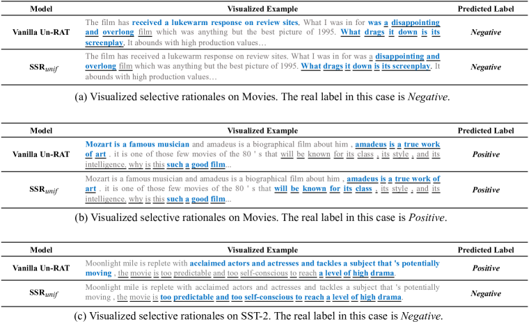
Figure 6: A visualized performance of extracted rationales with different methods.

In Figure 6(a), where the label is Negative, we find although both Vanilla Un-RAT and $\textmd{SSR}_{unif}$ predict the label as Negative correctly, Vanilla Un-RAT still extracts shortcuts as rationales. Specifically, “received a lukewarm response” is the shortcuts, where human being judges a movie is not influenced by other reviews. $\textmd{SSR}_{unif}$ avoids these shortcuts, but Vanilla Un-RAT extracts these as rationales.

In Figure 6(b), where the label is Positive, we observe find although both Vanilla Un-RAT and $\textmd{SSR}_{unif}$ predict the label as Positive correctly, Vanilla Un-RAT still extracts shortcuts as rationales. Specifically, “Mozart is a famous musician” is the shortcuts. Although Mozart was a great musician, it has no relevance to how good his biographical film is. Our $\textmd{SSR}_{unif}$ avoids these shortcuts, but Vanilla Un-RAT extracts these as rationales.

In Figure 6(c), where the label is Negative, we can find $\textmd{SSR}_{unif}$ predicts the label as Negative correctly but Vanilla Un-RAT fails. Specifically, since Vanilla Un-RAT relies on shortcuts in the data for prediction, when Vanilla Un-RAT is generalized to the OOD dataset (i.e., SST-2), the task performance decreases due to the changed data distribution. And some wrong rationales are extracted. Our $\textmd{SSR}_{unif}$, on the other hand, extracts the rationales accurately and predicts the task results correctly, indicating the effectiveness of exploring shortcuts to predict task results.

Appendix E Discussions of SSR and LLMs

Since SSR can mitigate the problem of utilizing shortcuts to compose rationales, our work can be applied to certain decision-making domains such as the judicial domain and the medical domain. In addition, although Large Language Models (LLMs) has achieved remarkable results recently, most LLMs (e.g. Chatgpt (Ouyang et al., 2022; OpenAI, 2023) and Claude (Anthropic, 2023)) need to be called as APIs. It cannot be used in privacy and security critical systems such as the judicial system. Our approach is much easier to deploy locally, ensuring privacy and improving explainability. Meanwhile, SSR is a model-agnostic approach, and we can replace BERT in SSR with opened LLMs (e.g., LLaMA (Touvron et al., 2023)) to achieve high performance.

SSR offers a solution for offering explanations in text classification tasks. For LLMs, in the autoregressive generation, we can view the prediction of each token as a text classification task, with the number of categories matching the vocabulary size. By generating an explanation for each token, we can gradually explain the output of a LLM. Nevertheless, effectively applying SSR to explain LLMs remains a formidable challenge. We are committed to further researching and exploring this area as a primary focus of our future work.

References

- Alemi et al. (2017) Alexander A. Alemi, Ian Fischer, Joshua V. Dillon, and Kevin Murphy. Deep variational information bottleneck. In 5th International Conference on Learning Representations, ICLR 2017, Toulon, France, April 24-26, 2017, Conference Track Proceedings, 2017.
- Anthropic (2023) Anthropic. Introducing claude. Anthropic Blogs, 2023. URL https://www.anthropic.com/index/introducing-claude.
- Antognini & Faltings (2021) Diego Antognini and Boi Faltings. Rationalization through concepts. In Findings of the Association for Computational Linguistics: ACL/IJCNLP2021, Online Event, August 1-6, 2021, 2021.
- Antognini et al. (2021) Diego Antognini, Claudiu Musat, and Boi Faltings. Multi-dimensional explanation of target variables from documents. In Proceedings of the AAAI Conference on Artificial Intelligence, 2021.
- Bao et al. (2018) Yujia Bao, Shiyu Chang, Mo Yu, and Regina Barzilay. Deriving machine attention from human rationales. In Proceedings of the 2018 Conference on Empirical Methods in Natural Language Processing, 2018.
- Bastings et al. (2019) Jasmijn Bastings, Wilker Aziz, and Ivan Titov. Interpretable neural predictions with differentiable binary variables. In Proceedings of the 57th Annual Meeting of the Association for Computational Linguistics (ACL), July 2019.
- Bhat et al. (2021) Meghana Moorthy Bhat, Alessandro Sordoni, and Subhabrata Mukherjee. Self-training with few-shot rationalization: Teacher explanations aid student in few-shot nlu. Proceedings of the 2021 Conference on Empirical Methods in Natural Language Processing (EMNLP), 2021.
- Carton et al. (2022) Samuel Carton, Surya Kanoria, and Chenhao Tan. What to learn, and how: Toward effective learning from rationales. In Smaranda Muresan, Preslav Nakov, and Aline Villavicencio (eds.), Findings of the Association for Computational Linguistics: ACL 2022, 2022.
- Chan et al. (2022) Aaron Chan, Maziar Sanjabi, Lambert Mathias, Liang Tan, Shaoliang Nie, Xiaochang Peng, Xiang Ren, and Hamed Firooz. Unirex: A unified learning framework for language model rationale extraction. In International Conference on Machine Learning, pp. 2867–2889. PMLR, 2022.
- Chang et al. (2019) Shiyu Chang, Yang Zhang, Mo Yu, and Tommi Jaakkola. A game theoretic approach to class-wise selective rationalization. Advances in Neural Information Processing Systems (NeurIPS), 32, 2019.
- Chang et al. (2020) Shiyu Chang, Yang Zhang, Mo Yu, and Tommi S. Jaakkola. Invariant rationalization. In Proceedings of the 37th International Conference on Machine Learning, (ICML), 2020.
- Chen & Ji (2020) Hanjie Chen and Yangfeng Ji. Learning variational word masks to improve the interpretability of neural text classifiers. In Proceedings of the 2020 Conference on Empirical Methods in Natural Language Processing, EMNLP 2020, Online, November 16-20, 2020, pp. 4236–4251, 2020.
- Clark et al. (2019) Christopher Clark, Kenton Lee, Ming-Wei Chang, Tom Kwiatkowski, Michael Collins, and Kristina Toutanova. BoolQ: Exploring the surprising difficulty of natural yes/no questions. In Proceedings of the 2019 Conference of the North American Chapter of the Association for Computational Linguistics: Human Language Technologies, Volume 1 (Long and Short Papers), 2019.
- (14) Jacob Devlin, Ming-Wei Chang, Kenton Lee, and Kristina Toutanova. Bert: Pre-training of deep bidirectional transformers for language understanding. In Proceedings of the 2019 Conference of the North American Chapter of the Association for Computational Linguistics (NAACL), pp. 4171–4186.
- DeYoung et al. (2020) Jay DeYoung, Sarthak Jain, Nazneen Fatema Rajani, Eric Lehman, Caiming Xiong, Richard Socher, and Byron C. Wallace. ERASER: A benchmark to evaluate rationalized NLP models. In Proceedings of the 58th Annual Meeting of the Association for Computational Linguistics, ACL 2020, Online, July 5-10, 2020, 2020.
- Hendrycks et al. (2020) Dan Hendrycks, Xiaoyuan Liu, Eric Wallace, Adam Dziedzic, Rishabh Krishnan, and Dawn Song. Pretrained transformers improve out-of-distribution robustness. In Proceedings of the 58th Annual Meeting of the Association for Computational Linguistics, 2020.
- Huang et al. (2021) Yongfeng Huang, Yujun Chen, Yulun Du, and Zhilin Yang. Distribution matching for rationalization. In Thirty-Fifth AAAI Conference on Artificial Intelligence, (AAAI), 2021.
- Jang et al. (2017) Eric Jang, Shixiang Gu, and Ben Poole. Categorical reparametrization with gumble-softmax. In International Conference on Learning Representations (ICLR). OpenReview. net, 2017.
- Johnson et al. (2019) Jeff Johnson, Matthijs Douze, and Hervé Jégou. Billion-scale similarity search with gpus. IEEE Transactions on Big Data, 7(3):535–547, 2019.
- Khashabi et al. (2018) Daniel Khashabi, Snigdha Chaturvedi, Michael Roth, Shyam Upadhyay, and Dan Roth. Looking beyond the surface: A challenge set for reading comprehension over multiple sentences. In Proceedings of the 2018 Conference of the North American Chapter of the Association for Computational Linguistics: Human Language Technologies, Volume 1 (Long Papers), pp. 252–262, 2018.
- Lakhotia et al. (2021) Kushal Lakhotia, Bhargavi Paranjape, Asish Ghoshal, Scott Yih, Yashar Mehdad, and Srini Iyer. FiD-ex: Improving sequence-to-sequence models for extractive rationale generation. In Proceedings of the 2021 Conference on Empirical Methods in Natural Language Processing, 2021.
- Lehman et al. (2019) Eric Lehman, Jay DeYoung, Regina Barzilay, and Byron C. Wallace. Inferring which medical treatments work from reports of clinical trials. In Proceedings of the 2019 Conference of the North American Chapter of the Association for Computational Linguistics: Human Language Technologies, Volume 1 (Long and Short Papers), 2019.
- Lei et al. (2016) Tao Lei, Regina Barzilay, and Tommi Jaakkola. Rationalizing neural predictions. In Proceedings of the 2016 Conference on Empirical Methods in Natural Language Processing (EMNLP), 2016.
- Li et al. (2022a) Dongfang Li, Baotian Hu, Qingcai Chen, Tujie Xu, Jingcong Tao, and Yunan Zhang. Unifying model explainability and robustness for joint text classification and rationale extraction. In Proceedings of the AAAI Conference on Artificial Intelligence, volume 36, pp. 10947–10955, 2022a.
- Li et al. (2022b) Haoyang Li, Ziwei Zhang, Xin Wang, and Wenwu Zhu. Learning invariant graph representations for out-of-distribution generalization. In Advances in Neural Information Processing Systems, 2022b.
- Liu et al. (2022) Wei Liu, Haozhao Wang, Jun Wang, Ruixuan Li, Chao Yue, and Yuankai Zhang. Fr: Folded rationalization with a unified encoder. Advances in neural information processing systems (NeurIPS), 2022.
- Liu et al. (2023) Wei Liu, Jun Wang, Haozhao Wang, and Ruixuan Li. D-separation for causal self-explanation. Advances in Neural Information Processing Systems, 2023.
- Loshchilov & Hutter (2019) Ilya Loshchilov and Frank Hutter. Decoupled weight decay regularization. In 7th International Conference on Learning Representations, ICLR 2019, New Orleans, LA, USA, May 6-9, 2019. OpenReview.net, 2019.
- Maas et al. (2011) Andrew Maas, Raymond E Daly, Peter T Pham, Dan Huang, Andrew Y Ng, and Christopher Potts. Learning word vectors for sentiment analysis. In Proceedings of the 49th annual meeting of the association for computational linguistics: Human language technologies, pp. 142–150, 2011.
- OpenAI (2023) OpenAI. Introducing chatgpt. OpenAI Blogs, 2023. URL https://openai.com/blog/chatgpt.
- Ouyang et al. (2022) Long Ouyang, Jeffrey Wu, Xu Jiang, Diogo Almeida, Carroll Wainwright, Pamela Mishkin, Chong Zhang, Sandhini Agarwal, Katarina Slama, Alex Ray, et al. Training language models to follow instructions with human feedback. Advances in Neural Information Processing Systems, 35:27730–27744, 2022.
- Pang & Lee (2004) Bo Pang and Lillian Lee. A sentimental education: Sentiment analysis using subjectivity summarization based on minimum cuts. Proceedings of the 42th Annual Meeting of the Association for Computational Linguistics (ACL), 2004.
- Paranjape et al. (2020) Bhargavi Paranjape, Mandar Joshi, John Thickstun, Hannaneh Hajishirzi, and Luke Zettlemoyer. An information bottleneck approach for controlling conciseness in rationale extraction. In Proceedings of the 2020 Conference on Empirical Methods in Natural Language Processing (EMNLP), November 2020.
- Pruthi et al. (2020) Danish Pruthi, Bhuwan Dhingra, Graham Neubig, and Zachary C. Lipton. Weakly- and semi-supervised evidence extraction. In Findings of the Association for Computational Linguistics: EMNLP 2020, 2020.
- Sha et al. (2021) Lei Sha, Oana-Maria Camburu, and Thomas Lukasiewicz. Learning from the best: Rationalizing prediction by adversarial information calibration. In Proceedings of the 35th AAAI Conference on Artificial Intelligence (AAAI), 2021.
- Socher et al. (2013) Richard Socher, Alex Perelygin, Jean Wu, Jason Chuang, Christopher D Manning, Andrew Y Ng, and Christopher Potts. Recursive deep models for semantic compositionality over a sentiment treebank. In Proceedings of the 2013 conference on empirical methods in natural language processing, 2013.
- Thorne et al. (2018) James Thorne, Andreas Vlachos, Christos Christodoulopoulos, and Arpit Mittal. Fever: a large-scale dataset for fact extraction and verification. arXiv preprint arXiv:1803.05355, 2018.
- Touvron et al. (2023) Hugo Touvron, Thibaut Lavril, Gautier Izacard, Xavier Martinet, Marie-Anne Lachaux, Timothée Lacroix, Baptiste Rozière, Naman Goyal, Eric Hambro, Faisal Azhar, Aurelien Rodriguez, Armand Joulin, Edouard Grave, and Guillaume Lample. Llama: Open and efficient foundation language models. arXiv preprint arXiv:2302.13971, 2023.
- Williams (1992) Ronald J Williams. Simple statistical gradient-following algorithms for connectionist reinforcement learning. Machine learning, 1992.
- Wu et al. (2022) Ying-Xin Wu, Xiang Wang, An Zhang, Xiangnan He, and Tat seng Chua. Discovering invariant rationales for graph neural networks. In ICLR, 2022.
- Yu et al. (2019) Mo Yu, Shiyu Chang, Yang Zhang, and Tommi S Jaakkola. Rethinking cooperative rationalization: Introspective extraction and complement control. In Empirical Methods in Natural Language Processing (EMNLP), 2019.
- Yu et al. (2021) Mo Yu, Yang Zhang, Shiyu Chang, and Tommi Jaakkola. Understanding interlocking dynamics of cooperative rationalization. Advances in Neural Information Processing Systems (NeurIPS), 34, 2021.
- Yue et al. (2022a) Linan Yue, Qi Liu, Yichao Du, Yanqing An, Li Wang, and Enhong Chen. Dare: Disentanglement-augmented rationale extraction. In Advances in Neural Information Processing Systems, 2022a.
- Yue et al. (2022b) Linan Yue, Qi Liu, Li Wang, Yanqing An, Yichao Du, and Zhenya Huang. Interventional rationalization. 2022b.
- Yue et al. (2024) Linan Yue, Qi Liu, Ye Liu, Weibo Gao, Fangzhou Yao, and Wenfeng Li. Cooperative classification and rationalization for graph generalization. In Proceedings of the ACM Web Conference 2024, 2024.