Turbulence from First Principles

Abstract

We provide a first-principles approach to turbulence by employing the electrodynamics of continuous media at the viscous limit to recover the Navier-Stokes equations. We treat oscillators with two orthogonal angular momenta as a spin network with properties applicable to the Kolmogorov-Arnold-Moser (KAM) theorem. The microscopic viscous limit has an irreducible representation that includes $O(3)$ expansion terms for a radiation-dominated fluid with a Friedmann–Lemaître–Robertson–Walker (FLRW) metric, equivalent to an oriented toroidal de Sitter space. The sum of particle velocity and pressure flux are conserved on the hypergeometric $n$-tori with stochastic boundary conditions. The turbulence solution in $\mathbb{R}^{3,1}$ lies on 6-choose-3 de Sitter intersections of three orthogonal $n$-tori.

Energy cascade describes the process of momentum transfer from large fluid rotations into ever smaller scale rotations. Kolmogorov scaling applies to the inertial sub-range of the power spectrum and provides a universal scaling law in which the energy contained within the domain of the eddy is proportional to its characteristic length scale $l$ and its wave number $k=l^{-1}$. The characteristic energy of the eddy ensemble $E$ is, $E(k)=\alpha\varepsilon^{2/3}k^{-5/3}$, where $\varepsilon$ is the ensemble energy dissipation rate and $\alpha$ is a constant.[OW19]. In his seminal 1941 statistical approach Kolmogorov assumed local isotropy of fluid pulsations in the medium being, a) equipped with the homogeniety property,[Kol91] and, b) this property being invariant under reflection and rotation transformations. In his work the velocity field was expanded to the second order and transformations evaluated at the high frequency, homogeneous boundary condition.

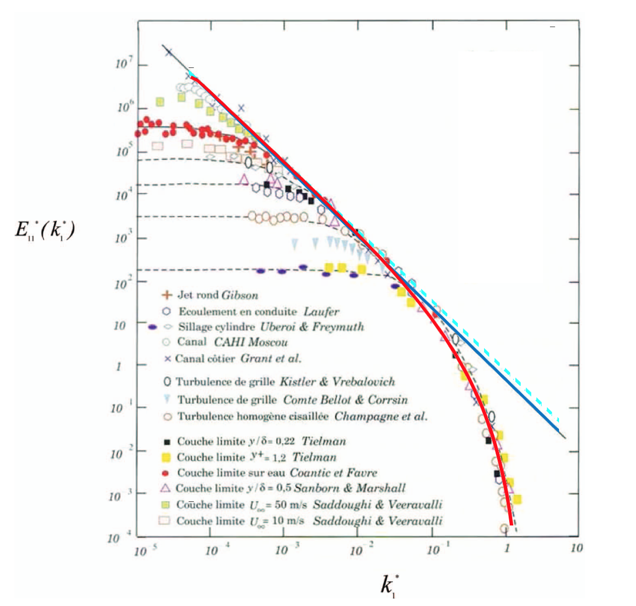
Figure 1: Comparison of our analytic result (red line) to empirical energy cascade in turbulence. Power spectrum of a fluid exhibits Kolmogorov scaling (blue solid line) in the inertial subrange before viscous effects dominate at high wavenumber, $k$. Our result converges on the golden ratio inertial subrange (dashed cyan). $E^{*}_{11}(k)$ is the normalised longitudinal energy spectra of the eddy domain ensemble with normalized wavevector $k^{*}$. The viscous scaling solution was evaluated using higher order terms of the velocity field to $O(3)$. 1-D turbulence spectrum data for various Taylor micro-scale Reynolds numbers with a fitted (dashed) curve adapted from [Cha00, ADD14].

The motivation.

Including third order expansion terms of the velocity field allows for the assessment of turbulence within the framework of the complete set of polarizations, applicable to any continuous media.[DT90, DMS00, Pap+16] We may gain insight into the reverse energy cascade process in which self-organisation takes place and identify phase transition mechanisms of any medium in motion provided that Maxwell’s equations are relevant at some scale. The phenomenon of intermittency at high wavenumber is closely related and may be assessed using a multi-fractal framework despite the fact that a first-principles solution has remained elusive.[SV10, PPB] Similarly, the shell model of magneto-hydrodynamic turbulence has enjoyed some success in 2D and (limited) 3D regimes [PSF13] by employing a quasi-condensed matter approach with, however, some paradoxical results. Recent stochastic approaches to model 1D turbulence with small viscosity appear successful[Kuk22] and consistent with [Kol91] but fail with the introduction of viscosity. We approach the problem from the high viscosity, heat-death limit by employing the toroid polarization of the Lorentz invariant two-potential formalism. The subtle difference between the two approaches being, at the high-frequency limit, the resolution of the $O(2)$ velocity field corresponds to linear pulsations wheres the $O(3)$ expansion includes the resolution-limit rotation and inherently includes viscous effects and the motion thereof.
Instead of using the K41 assumption of isotropy we evaluate the angular momentum dispersion ratio $\frac{\dot{q}_{\parallel}}{\dot{q}_{\perp}}\big{|}_{k_{max}}$assuming degeneracy of the classical motion of charged particles’ oscillation. Specifically, $r_{min}$ in this limit is the smallest accessible radius traced by a bound-charge electric displacement vector $\vec{P}$ where the total electric flux displacement vector is $\vec{D}$, following the convention of [DMS00],

$$\vec{D}=\vec{E}+4\pi\vec{P}$$

The microscopic electric field flux vector $\vec{E}$ contributes to the macroscopic pressure scalar as its integrated over $4\pi$.[Bra65] Similarly, viscosity is the macroscopic property directly related to the rate of strain tensor,

$$D_{ij}^{(2)}=\int{\vec{r}_{i}\vec{P}_{j}+\vec{r}_{j}\vec{P}_{i}-\frac{2}{3}(\vec{r}\cdot\vec{P})\delta_{ij}}d\vec{r}$$ (1)

where $\vec{r_{x}}=\Delta x$ as shown in fig. 3.

Let a unit cylinder have radius $R+r$ and height $2r$ with an embedded torus with minor and major radius $r_{0}$ and $R$ respectively. The configuration for maximum shear strain evaluated at the cylinder surface defined by a periodic surface $x_{0},y_{0}$ is shown in fig 3. The volumetric toroid moment for a purely poloidal current confined to the torus surface is,

$$\frac{\vec{T}^{(m)}}{V}=\frac{|\vec{P}|\pi Rr}{c}$$ (2)

For a fixed poloidal current magnitude we can achieve maximum viscosity $\int_{G}|D_{ij}^{(2)}|d^{3}r$ in the domain $G\in\mathbb{T}^{2}$ for the irreducible configuration shown in fig. 3. For a system representation containing only angular momentum the spin networks closed in $\mathbb{R}^{3}$ have a characteristic ensemble energy $\oint{{D}^{(2)}_{ij\parallel}}dl$ such that flux field lines are always closed at some scale. The picture is no different to a spin network [RV14] where angular momentum packets are irreducible to a choice of spin-1/2 or spin-0 on a discrete space-time. $\mathbb{T}^{2}$ is a natural coordinate frame to start in in order to describe the oriented (in $\hat{x},\hat{y}$ or $\hat{z}$) viscous dissipation properties.

From KAM theory: Implying some characteristics of invariant tori from the KAM theorem the stability of orbits under perturbation leads to a dispersion ratio $\dot{D}^{(2)}_{ij\parallel}/\dot{D}^{(2)}_{ij\perp}$ being simply half the winding number of the most statistically observable toroidal orbit, $\frac{k_{\parallel}}{2k{\perp}}$. The rate at which degeneracy is reached is proportional to the irrationality of the winding number, the golden ratio being the most irrational.[Irw+] We can intuitively use the concept of nearest-neighbour tori in a periodic packing to assess the momentum transfer in analogy to the multi-fractal approach[BV22]. Longitudinal momentum transfer can occur only via (1) between stacked tori, whereas half of the transverse contact area is shielded due to the inward converging geometry of the horn torus, $\frac{r}{r+R}\rightarrow\frac{1}{2}$ when $n\rightarrow\infty$. For a fully developed, degenerate system of orbits at $k_{max}$,

$$\frac{\dot{D}^{(2)}_{ij\parallel}}{\dot{D}^{(2)}_{ij\perp}}=\frac{1+\sqrt{5}}{4}$$ (3)

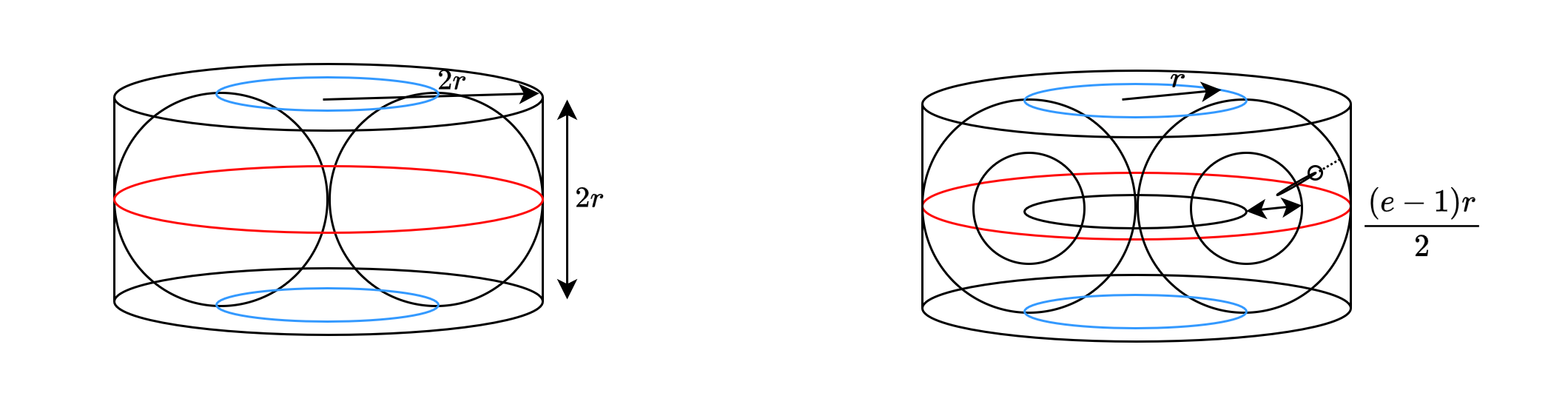
Figure 2: Left, unit cylinder with embedded torus showing longitudinal contact sites (blue). Right, fractally enveloping ring tori converge onto a dense n-dimensional horn torus filling the unit cylinder when $r_{n+1}=\frac{r_{n}(e-1)}{2},n\rightarrow\infty$

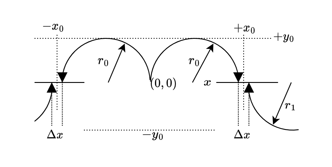
Figure 3: For paths traced by the electric displacement vector $\vec{P}$ the maximum dissipation via viscous effects occurs in the limit $\Delta x\rightarrow r_{\text{bound}}$ and $r_{0}=r_{1}=k_{max}^{-1}$. Toroidal moments arise from octupole ($O(3)$ irreducible terms and higher) as in the configuration shown above, having four dipoles centred about $\pm x_{0}$. They equally arise from the in-plane rotation of quadrupole moments, i.e. eq (1) in a rotating frame. Angular momentum is transported via eq (1) through either $\pm y_{0}$ surface ($\parallel T^{(m)}$), or the $\pm x_{0}$ surface ($\perp T^{(m)}$).

The invariant rotation of EM fields and sources is determined by a self-consistent formalism [DMS00]. The mechanism that achieves this is the $U(1)$ dyality symmetry[HB71] which introduces the scale dependence of EM interactions via the higher order toroidal polarized terms due to the closed EM field lines.[BD01] The domain $G$ may be constructed with fractally enveloping tori $k_{-}$ and fractally contained tori $k_{+}$ up to $k_{max}$ for a single particle with two orthogonal angular momenta $k_{n},k_{n+1}$. The Fourier-containing chart for any path interval $\int{\vec{D}dt}$ in the domain $G$ onto $\mathbb{R}^{3}$ happens to correspond exactly with the FLRW-based toroidal de Sitter flat chart,[NY19]

$$ds^{2}= -dt^{2}+e^{2Rt}d\vec{R}^{2}$$ (4)

where the scaling constant $R$ is proportional to the radius of the particle (ensemble) path $r$ on the oriented $\mathbb{T}^{2}$ space with coordinates $\vec{R}$. The dyality relation gives the $n$th-order multipole of the fractally enveloping $n_{-}$, and containing $n_{+}$ toroids.

$${R}_{j} =\frac{2}{(e-1)}\frac{(n_{j}-n_{min})!}{k_{j}-k_{min}}-\frac{e-1}{2(n_{max}-n_{j})!(k_{max}-k_{j})},n\in\mathbb{Z}^{+},k\in(0,1]$$ (5)

$$\vec{T}_{z}^{n(m),(e)} =\vec{T}_{z}^{n+1(e),(m)}=\nabla_{z}\times{\vec{T}^{n-1(e),(m)}}$$ (6)

$$\nabla\times\vec{T}^{(e),(m)} =\pm\Big{(}\frac{1}{c}\frac{\partial\vec{T}^{(m),(e)}}{\partial t}+\nabla\phi^{(m),(e)}\Big{)}$$ (7)

Superscript ($m$) denotes the magnetic toroidal moment and ($e$) denotes the electric toroid moment. [DT90] The spatio-temporal interchange between closed magnetic and electric field lines and between hypersurfaces is evident in (6) and (7).
The initial position, momentum and pressure flux of the $j$th particle (or ensemble of particles) is defined on a single hypersurface $n_{j}$, in toroidal coordinates,

$$\vec{R}_{j0}^{2}=e^{\phi_{0}}\big{(}(e-1)R_{0}\big{)}^{2}+\big{(}e^{\phi_{1}i}R_{1}+...+e^{\phi_{n_{j}}i}R_{n_{j}}\big{)}^{2}$$ (8)

All-order toroidal polarized electromagnetic interactions may be solved self-consistently on 6-choose-3 intersections of three orthogonal FLRW (toroidal de Sitter) space corresponding to a radiation-dominated fluid at the microscopic boundary condition of viscous heat-death. The scaling parameters are derived from $k_{max}$ and $n_{max}$ as properties of the medium, $k_{min}$ and $n_{min}$ as properties of the domain $G$ and $n_{j},k_{j}$ as the properties of the particle (or ensemble of particles) under consideration. The total flux displacement $\vec{D}$ is conserved on these intersections with emergent stochastic properties.

Anzats.

The solution of the Navier-Stokes equations exists at the stochastic intersections of three orthogonal toroidal de Sitter spaces described by (4), (5), (6), (7) with the dispersion relation (3) of the degenerate spin-oscillator system.

Derivation.

The toroidal momentum de Sitter space flat chart metric is (4). The oriented toroidal coordinate space $\mathbb{T}^{2}$ maps to the oriented toroidal phase space $\mathbb{T}^{1}$ for the fractal 2D-harmonic oscillator set. The Hamiltonian for the motion of a particle on a torus in fractal tori phase space is given by,

$$\Omega=\frac{q_{\phi_{n}}^{2}}{2m}+\frac{q_{\phi_{n-1}}^{2}}{2m}$$

where $q_{\phi_{n}}$ and $q_{\phi_{n-1}}$ are the conjugate momenta corresponding to the angular coordinates $\phi_{n}$ and $\phi_{n-1}$, respectively to form a torus, and $m$ is the mass of the particle containing the bound charge. The ray equations for this spin-orbit system correspond to the free motion of charged particles on tori in coordinate space,

$$\frac{d\phi_{n}}{dt}=\frac{q_{\phi_{n}}}{m}, \quad\frac{d\phi_{n-1}}{dt}=\frac{q_{\phi_{n-1}}}{m},$$

$$\frac{dq_{\phi_{n}}}{dt}=0, \quad\frac{dq_{\phi_{n-1}}}{dt}=0$$

Any particle in $\mathbb{R}^{3}$ lives on the $n$th toroidal hypersurface given a momentum (5) and position (8). The electromagnetic scaling inter-dependency of (6) and (7) is made explicit with the fractally enveloping torus minor and major radii,

$$r_{n}=k_{n}^{-1}=\frac{R_{n}(e-1)}{2}$$

so that the entire space (of a 2D spin-orbit system) can be described by two independent complex constants of motion, [JS06]

$$F_{(n-1)}=R_{n}e^{i2k_{n}t/(e-1)},\quad F_{n}=r_{n}e^{ik_{n}t}$$ (9)

For invariant tori in phase space a 2D oscillator has incommensurate frequencies $\frac{\omega_{k+1}}{\omega_{k}}$ corresponding to an irrational winding number and is most robust to perturbation. The resulting dispersion ratio is (3).

The Ohmic field flux $\vec{E}$ is directly proportional to the pressure flux $\vec{p}$, not to be confused with the electric bound-charge displacement vector $\vec{P}$, where the total displacement flux is,

$$\vec{D}=\vec{E}+4\pi\vec{P}=\vec{p}+4\pi\vec{u}dt$$ (10)

The current configuration at the viscous heat-death boundary condition is defined as the microscopic magnetic dipole moment $\vec{M}_{z}\rightarrow 0$,[Bra65] evaluated at $n_{max},r_{min}$. In Cartesian coordinates and in the convention of [NBF18],

$$\frac{\vec{D}^{\prime}(\vec{R}(n_{max}-1))}{dt}=2\pi^{2}R\frac{\vec{D}(\vec{R}(n_{max}))}{dt}\text{rot}\hat{\mathbf{z}}\delta(r)\\ +\frac{\pi^{2}R}{8}\frac{\vec{D}(\vec{R}(n_{max}))}{dt}\left[2R^{2}(\nabla^{2}x+\nabla^{2}y)\right]\text{rot}\hat{\mathbf{z}}\delta(r)+O(r^{-4})$$ (11)

where $\vec{D}^{\prime}$ is the electric flux displacement vector of the bound charge with path curvature $\frac{2}{e-1}r_{min}$, corresponding to the penultimate cascade momentum. Similarly for $\vec{M}_{x}=\vec{M}_{y}\rightarrow 0$, at $k_{max}$ and $\text{rot}\hat{\mathbf{k}}\delta(r)=1,$ for $k=\{x,y,z\}$. Combining (10) into (11) gives three equations in the non-dimensional form. For $\hat{z}$,

$$\begin{split}\nabla_{y}^{2}-\nabla_{x}^{2}-\nabla_{z}^{2}=\Big{(}\frac{\vec{D}}{dt}\Big{)}^{-1}\Big{(}\frac{4\vec{D}^{\prime}\text{rot}\hat{\mathbf{z}}}{dt\pi^{2}R_{z}^{3}}\Big{)}&-\frac{8}{R_{z}^{2}}-\Big{(}\frac{\vec{D}}{dt}\Big{)}^{-1}\Big{(}\frac{4\vec{D}^{\prime}\text{rot}\hat{\mathbf{y}}}{dt\pi^{2}R_{y}^{3}}\Big{)}\\ &+\frac{8}{R_{y}^{2}}-\Big{(}\frac{\vec{D}}{dt}\Big{)}^{-1}\Big{(}\frac{4\vec{D}^{\prime}\text{rot}\hat{\mathbf{x}}}{dt\pi^{2}R_{x}^{3}}\Big{)}+\frac{8}{R_{x}^{2}}\end{split}$$ (12)

Continuing to evaluate the $z$ component, linear perturbations in $x$ and $y$ occur at the limit $R_{z}\rightarrow\infty$, similarly for all perturbations in the $z$ component (12),

$$\Bigg{[}\Bigg{]}_{y}-\Bigg{[}\Bigg{]}_{x}=\nabla_{x}^{2}-\nabla_{y}^{2},\begin{cases}R_{x}=R_{y}\\ R_{z}\rightarrow\infty\end{cases}$$ (13)

$$\Bigg{[}\Bigg{]}_{y}-\Bigg{[}\Bigg{]}_{z}=\nabla_{y}^{2}-\nabla_{z}^{2},\begin{cases}R_{y}=R_{z}\\ R_{x}\rightarrow\infty\end{cases}$$ (14)

$$\Bigg{[}\Bigg{]}_{z}-\Bigg{[}\Bigg{]}_{x}=\nabla_{z}^{2}-\nabla_{x}^{2},\begin{cases}R_{z}=R_{x}\\ R_{y}\rightarrow\infty\end{cases}$$ (15)

where,

$$\Bigg{[}\Bigg{]}_{j}=\Big{(}\frac{\vec{D}}{dt}\Big{)}^{-1}\Big{(}\frac{4\vec{D}^{\prime}\text{rot}\hat{\mathbf{j}}}{dt\pi^{2}R_{j}^{3}}\Big{)}-\frac{8}{R_{j}^{2}},\quad j\in\{x,y,z\}$$ (16)

The boundary conditions in (13), (14), (15) and (11) require alternately spanning the momentum spectrum assigning the degree of freedom to the scalar components and larger radius (enveloping) vector components $j^{\prime}$ in (10) to give the total solution for $\hat{x},\hat{y},\hat{z}$ (11). This constitutes a stochastic condition on (12).

$$\Bigg{[}\Bigg{]}_{j}-\Bigg{[}\Bigg{]}_{j^{\prime}}=-\nabla_{x}^{2}-\nabla_{y}^{2}-\nabla_{z}^{2},\quad j\in\{x,y,z\}$$ (17)

when,

$$ds_{x}=ds_{y},$$ (18)

$$ds_{y}=ds_{z},$$ (19)

$$ds_{z}=ds_{x}$$ (20)

Putting (17), (16) and (10) together we recover the first normalized, momentum-dependent Navier-Stokes equation,

$$\frac{\partial p}{p_{j}+4\pi\vec{u}_{j}}+\frac{4\partial\vec{u}\text{rot}\hat{j}}{R^{3}_{j}\pi^{2}(p_{j}+4\pi\vec{u}_{j})}=\frac{8}{R_{j}^{2}}-\Delta^{2}$$ (21)

since the RHS of (17) is repeated over $j=\{x,y,z\}$, either a completely static solution exists, or the divergence equation holds,

$$\Delta^{2}=0$$ (22)

The roots to the cubic (21) provide the set of solutions for the Navier-Stokes equations and may coincide with the fugacity of the system.[Lee09] Shown in fig. 4 the intersection of orthogonal de Sitter paths at $n_{max}$ allow for the solutions at the viscous limit, i.e. the local degeneracy of orbits and in the jerk frame. The interpretation of $p_{j}$ is the electric field flux in the direction ${j}\in\{x,y,z\}$ resulting from the momentum-dependent Coulomb interaction. The microscopic E field is equivalent to the microscopic pressure gradients in contrast to the macroscopic Ohmic field and pressure values; both scalar.

Setting $\vec{u}=0$ implies a limit to the pulsation magnitude and that it be proportional to the wave-vector as per [Kol91] method. Rewriting (21) with this condition,

$$\frac{4\partial\vec{u}\text{rot}\hat{x}}{R_{x}^{3}\pi^{2}}=\frac{8p_{x}}{R^{2}_{x}}-\Delta^{2}p_{x}-\partial p$$ (23)

$$\frac{4\partial\vec{u}\text{rot}\hat{y}}{R_{y}^{3}\pi^{2}}=\frac{8p_{y}}{R^{2}_{y}}-\Delta^{2}p_{y}-\partial p$$ (24)

$$\frac{4\partial\vec{u}\text{rot}\hat{z}}{R_{z}^{3}\pi^{2}}=\frac{8p_{z}}{R^{2}_{z}}-\Delta^{2}p_{z}-\partial p$$ (25)

where,

$$\frac{4\partial\vec{u}\text{rot}\hat{x}}{R_{x}^{3}\pi^{2}}+\frac{4\partial\vec{u}\text{rot}\hat{y}}{R_{y}^{3}\pi^{2}}=\frac{32\pi c\partial\mathbf{T}_{z}}{V^{2}}$$ (26)

is the $z$-oriented volumetric dissipation rate with units $\Big{[}\frac{C}{m^{2}s}\frac{1}{m^{3}}\Big{]}$ due to only the bound charge rotation and neglecting the contribution of electric field flux, differentiated by the use of $\mathbf{T}$ vice $\vec{T}^{(m)}$. Again using the intersection equalities from (13)-(15), (26) we can rewrite (23) in volumetric dissipation terms oriented in $x,y$ and $z$. For $z$;

$$\Delta^{2}(p_{x}-p_{y})=\frac{8(p_{x}-p_{y})}{R^{2}}-\frac{32\pi}{R^{3}}\Big{(}\frac{\partial\mathbf{T}_{z}}{V^{2}}\Big{)},\quad c=1,R_{x}=R_{y}=R$$ (27)

Further, we impose the condition,

$$\Delta^{2}(p_{x}-p_{y})=1$$ (28)

which implies the jerk frame at the viscous heat-death limit, i.e. as cascade energy is constantly dumped into the spin-oscillator system the flux-derived angular momentum must change. In contrast to [Kol91] this is a non-equilibrium condition. Completing the above process along $x$ and $y$ and choosing roots of $R$ in the positive time direction (see fig. 4), we can construct the energy cascade scale from the viscous heat death condition.

First, from the degeneracy assumption, the longitudinal dissipation rate from (3) is,

$$\frac{d\vec{D}}{dt}=\frac{k^{\frac{1+\sqrt{5}}{4}}}{4\pi}$$ (29)

Using only the $t_{+}$ roots of $R$ in (27) the de Sitter path interval of a closed loop about $b=\{\hat{x},\hat{y},\hat{z}\}\in\mathbb{R}^{3}$ becomes,

$$ds_{+}=\Bigg{(}16\pi^{2}dk^{-2\Big{(}{\frac{1+\sqrt{5}}{4}}\Big{)}}+dR_{b}(k,r_{min})^{2}e^{2dR_{b}(k,r_{min})}\Bigg{)}^{\frac{1}{2}}$$ (30)

where $R_{b}=\big{(}Im(R_{1})+Re(R_{2})+Re(R_{3})\big{)}^{\frac{1}{2}}$, the applicable root components are,

$$Im(R_{1})=2Im\Bigg{(}\frac{{2^{1/3}\left(\sqrt{3}\sqrt{27\pi^{2}p_{ab}^{4}-2p_{ab}^{3}}-9\pi p_{ab}^{2}\right)^{1/3}}}{{3^{2/3}p_{ab}}}\\ +\frac{{2^{2/3}}}{{3^{1/3}\left(\sqrt{3}\sqrt{27\pi^{2}p_{ab}^{4}-2p_{ab}^{3}}-9\pi p_{ab}^{2}\right)^{1/3}}}\Bigg{)}\\ Re(R_{2})=-Re\Bigg{(}\frac{2^{1/3}(1-i\sqrt{3})(\sqrt{3}\sqrt{27\pi^{2}p_{ab}^{4}-2p_{ab}^{3}}-9\pi p_{ab}^{2})^{1/3}}{3^{2/3}p_{ab}}\\ -\frac{2^{2/3}(1+i\sqrt{3})}{3^{1/3}(\sqrt{3}\sqrt{27\pi^{2}p_{ab}^{4}-2p_{ab}^{3}}-9\pi p_{ab}^{2})^{1/3}}\Bigg{)}\\ Re(R_{3})=-Re\Bigg{(}\frac{2^{1/3}(1+i\sqrt{3})(\sqrt{3}\sqrt{27\pi^{2}p_{ab}^{4}-2p_{ab}^{3}}-9\pi p_{ab}^{2})^{1/3}}{3^{2/3}p_{ab}}\\ -\frac{2^{2/3}(1+i\sqrt{3})}{3^{1/3}(\sqrt{3}\sqrt{27\pi^{2}p_{ab}^{4}-2p_{ab}^{3}}-9\pi p_{ab}^{2})^{1/3}}\Bigg{)}$$ (31)

where, $p_{ab}=\{(p_{x}-p_{y}),(p_{z}-p_{x}),(p_{y}-p_{z})\}$.

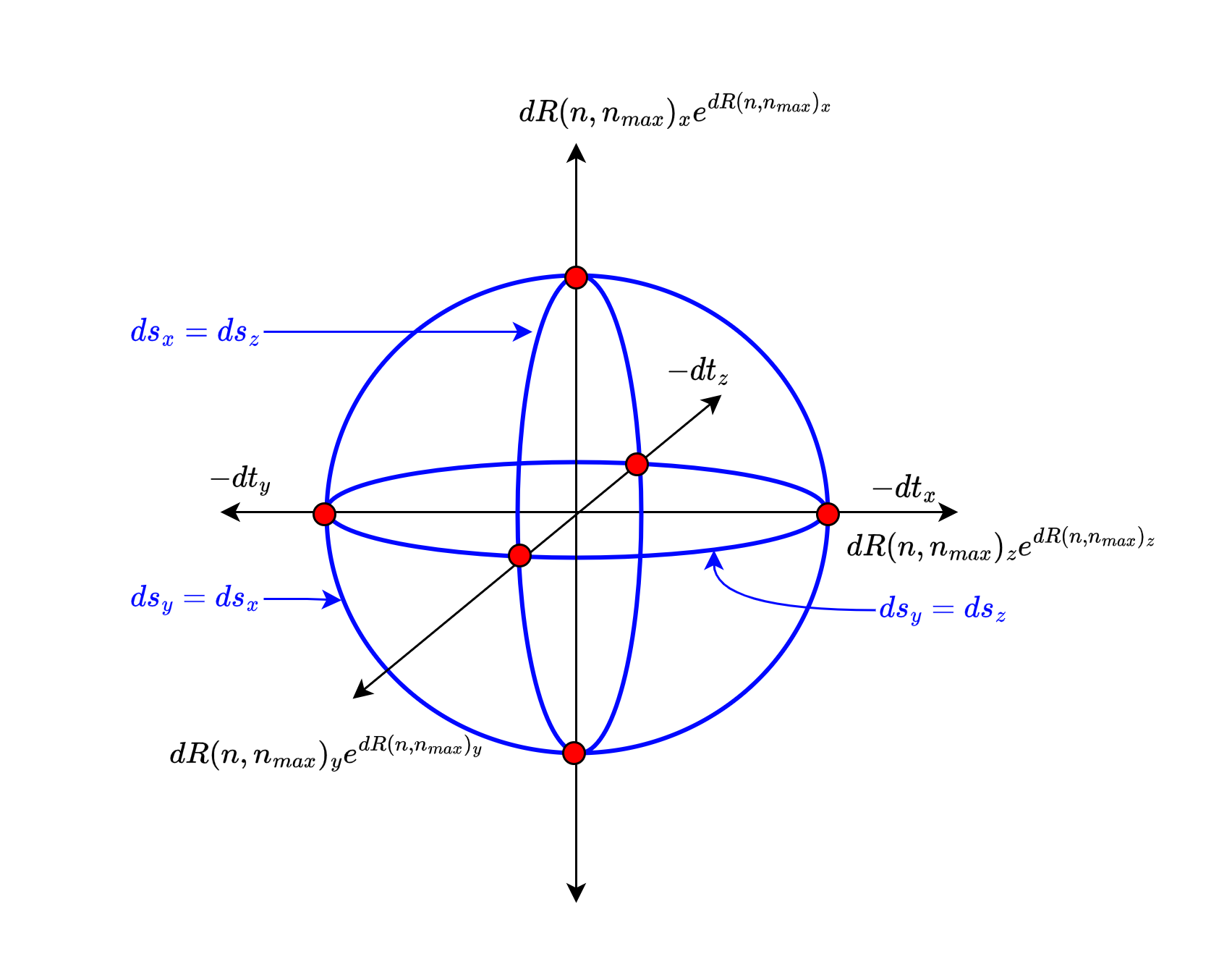
Figure 4: The $z$-oriented solutions of toroidal spin-oscillator spaces (red points) exist on hypersurfaces $dR_{z}e^{dR_{z}}$ that co-exist with 0, 1 or 2 independent time dimensions. We may interpret the opposing time directions associated with the $z$-hypersurface as an energy cascade balancing mechanism, or simply equal angular momentum dissipation rate into orthogonal directions, in this case $\hat{x}$ and $\hat{y}$. There are 3 positive time solutions and 2 time-independent solutions.

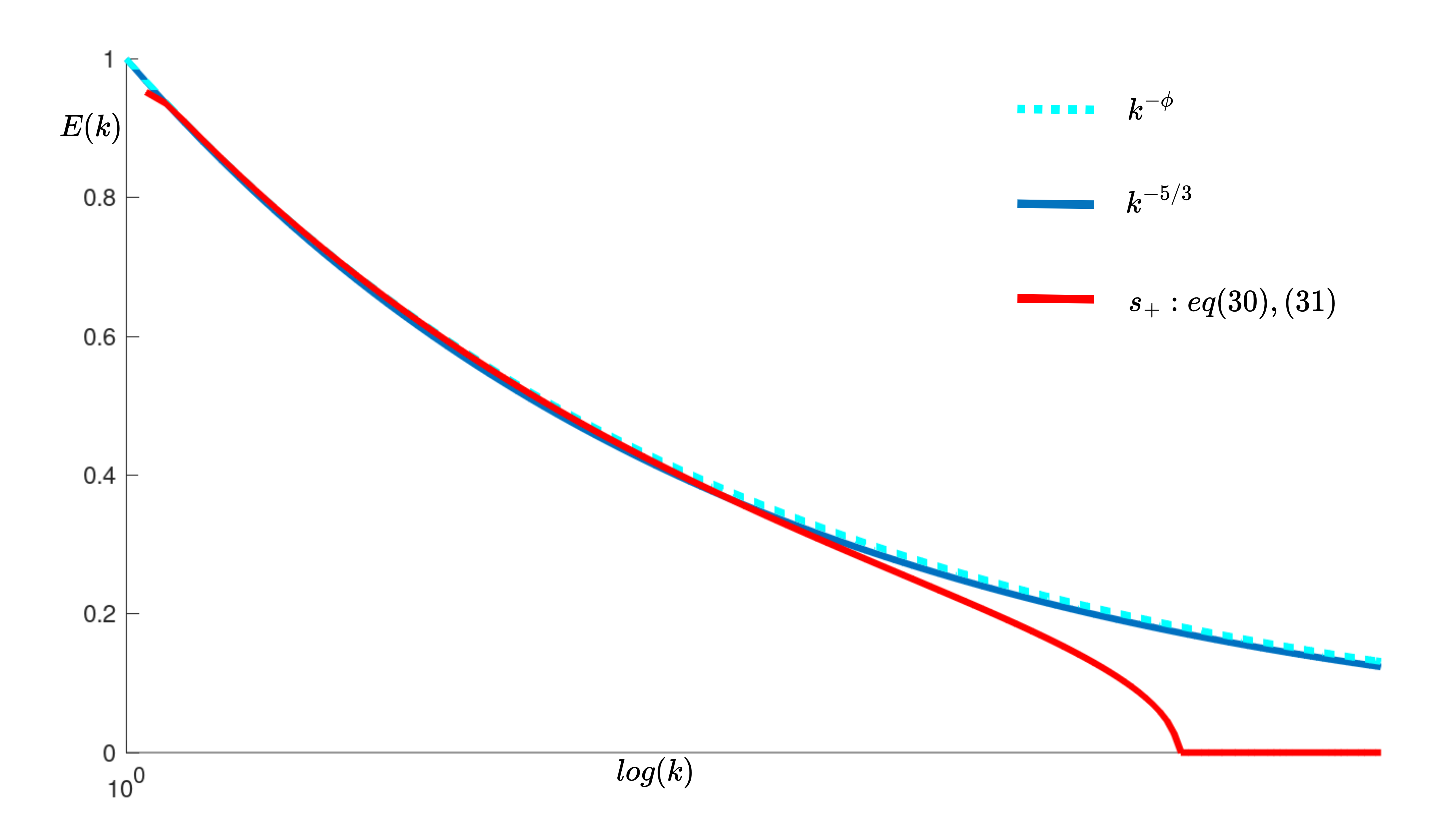
Figure 5: $O(2)$ Komologorov scaling law (blue) and $O(3)$ viscous energy cascade scale (red) given by the toroidal de Sitter path interval $s_{+}$ with momentum scaling parameter $R$. The inertial sub-range in our solution converges on the golden ratio exponent (dashed cyan) due to the degeneracy assumption of invariant tori in phase space. In the dissipative sub-range the volumetric dissipation rate is $\sim\mathbf{T}_{b}k^{6}$, from (27) where $\mathbf{T}_{b}$ is the microscopic magnetic toroidal susceptibility tensor.

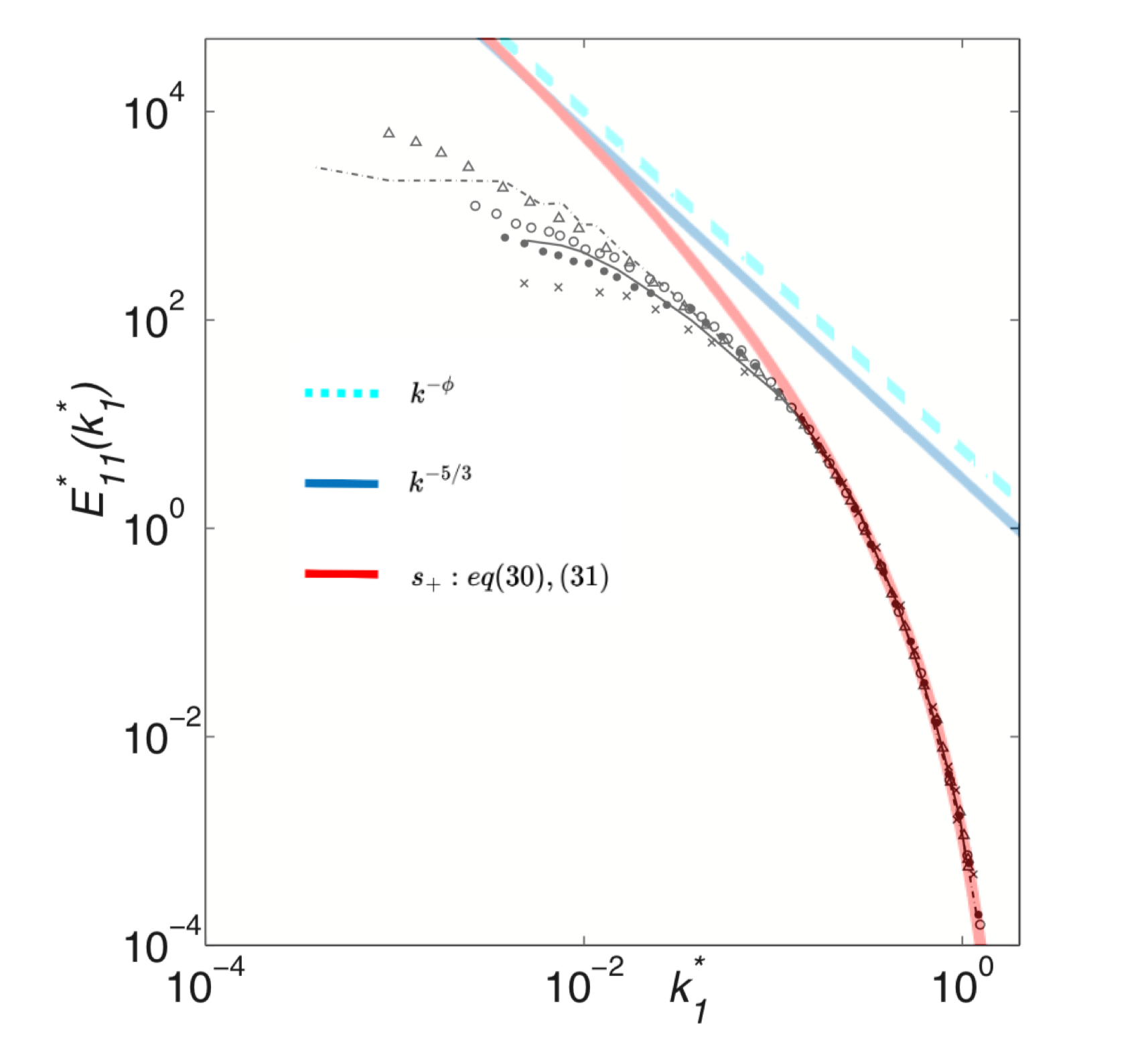
Figure 6: Normalized longitudinal spectra for various turbulence regimes and corresponding Taylor microscale Reynolds numbers, Re_λ. (x - Re_λ=40, dots - 67, solid line - 65, circles - 89, triangles - 139, dash-dot line - 130). Fitting the dissipative curve to the turbulence data provides qualitative insight into the longitudinal energy gap at various frequencies. Adpated from [ADD14].

Conclusion.

Having employed a condensed matter approach we evaluated the angular momentum transfer in a classical spin-network which allowed for the extension of Kolmogorov scaling into the viscous range. The assumption of degeneracy of classical orbits at a finite frequency were made allowing us to recover the momentum-normalized Navier-Stokes Equations (21), (22) from first principles. In doing so we also defined the space of solutions with the addition of the stochastic assumptions being applied to the cancellation of magnetic flux (quanta) in the jerk frame. The solution for the Navier-Stokes equation with suppressed intermittency are given by (30) and (31). $\Box$

References

- [Bra65] S.. Braginskii “Transport Processes in a Plasma” ADS Bibcode: 1965RvPP….1..205B In Reviews of Plasma Physics 1, 1965, pp. 205 URL: https://ui.adsabs.harvard.edu/abs/1965RvPP....1..205B
- [HB71] M.. Han and L.. Biedenharn “Manifest dyality invariance in electrodynamics and the cabibbo-ferrari theory of magnetic monopoles” In Il Nuovo Cimento A 2.2, 1971, pp. 544–556 DOI: 10.1007/BF02899873
- [DT90] V.. Dubovik and V.. Tugushev “Toroid moments in electrodynamics and solid-state physics” In Physics Reports 187.4, 1990, pp. 145–202 DOI: https://doi.org/10.1016/0370-1573(90)90042-Z
- [Kol91] Kolmogorov “The local structure of turbulence in incompressible viscous fluid for very large Reynolds numbers” In Proceedings of the Royal Society of London. Series A: Mathematical and Physical Sciences 434.1890, 1991, pp. 9–13 DOI: 10.1098/rspa.1991.0075
- [Cha00] Patrick Chassaing “Turbulence En Mécanique Des Fluides—Analyse Du Phénomène En Vue De Sa Modélisation Par l’ingénieur”, 2000
- [DMS00] V.. Dubovik, M.. Martsenyuk and Bijan Saha “Material equations for electromagnetism with toroidal polarizations” In Physical Review E 61.6, 2000, pp. 7087–7097 DOI: 10.1103/PhysRevE.61.7087
- [BD01] E N Bukina and V M Dubovik “Higher Vector Polarizations and Quasistationary Phenomena in Enveloping Tori” In Measurement Techniques 44, 2001, pp. 934–943 DOI: 10.1023/A:1013211806287
- [JS06] Jorge V. José and Eugene J. Saletan “Classical dynamics: a contemporary approach” Cambridge: Cambridge Univ. Press, 2006
- [Lee09] M Howard Lee “POLYLOGARITHMS AND LOGARITHMIC DIVERSION IN STATISTICAL MECHANICS” In ACTA PHYSICA POLONICA B 40.5, 2009, pp. 1279
- [SV10] Domingos S.. Salazar and Giovani L. Vasconcelos “Stochastic dynamical model of intermittency in fully developed turbulence” In Physical Review E 82.4, 2010, pp. 047301 DOI: 10.1103/PhysRevE.82.047301
- [PSF13] Franck Plunian, Rodion Stepanov and Peter Frick “Shell models of magnetohydrodynamic turbulence” In Physics Reports 523.1, 2013, pp. 1–60 DOI: 10.1016/j.physrep.2012.09.001
- [ADD14] R.. Antonia, L. Djenidi and L. Danaila “Collapse of the turbulent dissipative range on Kolmogorov scales” In Physics of Fluids 26.4, 2014, pp. 045105 DOI: 10.1063/1.4869305
- [RV14] Carlo Rovelli and Francesca Vidotto “Covariant Loop Quantum Gravity: An Elementary Introduction to Quantum Gravity and Spinfoam Theory” Cambridge University Press, 2014 DOI: 10.1017/CBO9781107706910
- [Pap+16] N. Papasimakis et al. “Electromagnetic toroidal excitations in matter and free space” In Nature Materials 15.3, 2016, pp. 263–271 DOI: 10.1038/nmat4563
- [NBF18] Nikita A. Nemkov, Alexey A. Basharin and Vassili A. Fedotov “Electromagnetic sources beyond common multipoles” In Physical Review A 98.2, 2018, pp. 023858 DOI: 10.1103/PhysRevA.98.023858
- [NY19] Tokiro Numasawa and Daisuke Yoshida “Global Spacetime Structure of Compactified Inflationary Universe” arXiv:1901.03347 [gr-qc, physics:hep-th] In Classical and Quantum Gravity 36.19, 2019, pp. 195003 DOI: 10.1088/1361-6382/ab38ed
- [OW19] David G. Ortiz-Suslow and Qing Wang “An Evaluation of Kolmogorov’s -5/3 Power Law Observed Within the Turbulent Airflow Above the Ocean” In Geophysical Research Letters 46.24, 2019, pp. 14901–14911 DOI: 10.1029/2019GL085083
- [BV22] Roberto Benzi and Angelo Vulpiani “Multifractal approach to fully developed turbulence” In Rendiconti Lincei. Scienze Fisiche e Naturali 33.3, 2022, pp. 471–477 DOI: 10.1007/s12210-022-01078-5
- [Kuk22] Sergei Kuksin “Kolmogorov’s theory of turbulence and its rigorous 1d model” In Annales mathématiques du Québec 46.1, 2022, pp. 181–193 DOI: 10.1007/s40316-021-00174-6
- [Irw+] Klee Irwin, Marcelo M Amaral, Raymond Aschheim and Fang Fang “Quantum Walk on a Spin Network and the Golden Ratio as the Fundamental Constant of Nature” URL: https://www.researchgate.net/publication/316554631_Quantum_Walk_on_a_Spin_Network_and_the_Golden_Ratio_as_the_Fundamental_Constant_of_Nature
- [PPB] Ali Poursina, Ali Pourjamal and Ali Bozorg “Stochastic Approach to Turbulence: A Comprehensive Review” DOI: arXiv:2211.12918v1