Transparent boundary condition and its effectively local approximation for the Schrödinger equation on a rectangular computational domain

Samardhi Yadav Samardhi@physics.iitd.ac.in Vishal Vaibhav vishal.vaibhav@gmail.com Department of Physics, Indian Institute of Technology Delhi, Hauz Khas, New Delhi–110016, India Optics and Photonics Center, Indian Institute of Technology Delhi, Hauz Khas, New Delhi–110016, India
Abstract

The transparent boundary condition for the free Schrödinger equation on a rectangular computational domain requires implementation of an operator of the form tiΓsubscript𝑡𝑖subscriptΓ\sqrt{\partial_{t}-i\triangle_{\Gamma}} where ΓsubscriptΓ\triangle_{\Gamma} is the Laplace-Beltrami operator. It is known that this operator is nonlocal in time as well as space which poses a significant challenge in developing an efficient numerical method of solution. The computational complexity of the existing methods scale with the number of time-steps which can be attributed to the nonlocal nature of the boundary operator. In this work, we report an effectively local approximation for the boundary operator such that the resulting complexity remains independent of number of time-steps. At the heart of this algorithm is a Padé approximant based rational approximation of certain fractional operators that handles corners of the domain adequately. For the spatial discretization, we use a Legendre-Galerkin spectral method with a new boundary adapted basis which ensures that the resulting linear system is banded. A compatible boundary-lifting procedure is also presented which accommodates the segments as well as the corners on the boundary. The proposed novel scheme can be implemented within the framework of any one-step time marching schemes. In particular, we demonstrate these ideas for two one-step methods, namely, the backward-differentiation formula of order 1 (BDF1) and the trapezoidal rule (TR). For the sake of comparison, we also present a convolution quadrature based scheme conforming to the one-step methods which is computationally expensive but serves as a golden standard. Finally, several numerical tests are presented to demonstrate the effectiveness of our novel method as well as to verify the order of convergence empirically.

keywords:
Transparent Boundary Conditions , Two-dimensional Schrödinger equation , Legendre-Galerkin Spectral Method , Convolution-Quadrature , Padé Approximants
journal: Journal of Computational Physics

Notations

The set of non-zero positive real numbers (\mathbb{R}) is denoted by +subscript\mathbb{R}_{+}. For any complex number ζ𝜁\zeta, Re(ζ)Re𝜁\operatorname{Re}(\zeta) and Im(ζ)Im𝜁\operatorname{Im}(\zeta) refer to the real and the imaginary parts of ζ𝜁\zeta, respectively. The open interval (1,1)11(-1,1) is denoted by 𝕀𝕀\mathbb{I}.

1 Introduction

This paper is devoted to the numerical solution of the two-dimensional free Schrödinger equation. The free Schrödinger equation and its various generalizations are of significant physical interest because they appear in many areas of application such as quantum mechanics, propagation of electromagnetic waves under paraxial approximation (or slow varying envelope approximation for pulse propagation in optical fibers) [1] and parabolic approximation to one-way propagation equation in underwater acoustics [2].

The initial value problem (IVP) corresponding to the free Schrödinger equation formulated on 2superscript2\mathbb{R}^{2} reads as

itu+u=0,(𝒙,t)2×+,formulae-sequence𝑖subscript𝑡𝑢𝑢0𝒙𝑡superscript2subscripti\partial_{t}u+\triangle u=0,\quad(\boldsymbol{x},t)\in\mathbb{R}^{2}\times\mathbb{R}_{+}, (1)

where the initial condition u(𝒙,0)=u0(𝒙)𝑢𝒙0subscript𝑢0𝒙u(\boldsymbol{x},0)=u_{0}(\boldsymbol{x}) is assumed to be compactly supported. In order to ensure the uniqueness of the solution, a Sommerfeld-like radiation condition at infinity is imposed [3]. For the numerical solution of this problem, we first need to choose a bounded computational domain, denoted by ΩisubscriptΩ𝑖\Omega_{i}, such that suppu0(𝒙)Ωisuppsubscript𝑢0𝒙subscriptΩ𝑖\operatorname*{supp}u_{0}(\boldsymbol{x})\subset\Omega_{i}. The next step is to determine appropriate boundary condition at the fictitious boundary (ΩisubscriptΩ𝑖\partial\Omega_{i}) such that the solution of the resulting initial-boundary value problem (IBVP) on ΩisubscriptΩ𝑖\Omega_{i} remains identical to that of original problem which is formulated on an unbounded domain. Such boundary conditions are known as the transparent boundary conditions (TBCs) which usually appear as Dirichlet-to-Neumann (DtN) or Neumann-to-Dirichlet (NtD) maps at the fictitious boundary [3]. In cases where it is possible to obtain these maps in a closed form, they turn out to be nonlocal with respect to space as well as time. The specific form of the transparent or nonreflecting boundary maps depend on the nature of the computational domain chosen. For practical reasons, the rectangular domain happens to be a natural choice for the computational domain. In this work, we address the challenges involved in choosing ΩisubscriptΩ𝑖\Omega_{i} to be a rectangular domain for which an exact nonreflecting boundary condition is known at a continuous level [4, 5]. In particular, we address the problem of designing a numerical scheme which provides a viable trade-off between computational complexity and accuracy when it comes to dealing with the nonlocal boundary maps at a discrete level. At the outset, let us state that the new algorithm presented in this work circumvents the need to store the entire history of the field on the boundary ΩisubscriptΩ𝑖\partial\Omega_{i} unlike the existing methods [4] such that the overall complexity turns out to be dominated by that of the linear solver for the interior problem. This effective localization of the DtN maps rely on a novel Padé approximant based approach that handles the corners adequately.

Several authors have contributed towards the formulation of exact TBCs for the two-dimensional Schrödinger equation [6, 7, 8, 9, 4, 10, 5]. Exact TBCs for the free Schrödinger equation on convex domains with smooth boundary was provided by Schädle [8] in terms of a single and a double layer potential. Han and Huang [9] provided the exact TBCs in terms of Hankel functions for the circular domain. For more general cases including the nonlinear Schrödinger equation on convex domains, Antoine et al. proposed some higher-order absorbing boundary conditions with the use of pseudo-differential operators [11, 12]. The transparent boundary operator for the Schrödinger equation on a rectangular domain has the form tiΓsubscript𝑡𝑖subscriptΓ\sqrt{\partial_{t}-i\triangle_{\Gamma}} where ΓsubscriptΓ\triangle_{\Gamma} is the Laplace-Beltrami operator. Note that these operators are nonlocal, both in time as well as space. To the best of our knowledge, an integral representation of this operator first appeared in [6] and more recently derived in [13, 5]. The earliest numerical implementation for the operator tiΓsubscript𝑡𝑖subscriptΓ\sqrt{\partial_{t}-i\triangle_{\Gamma}} was given by Menza [7] who introduced a Padé approximant based rational approximation for the complex square root function to obtain effectively local boundary conditions. However, this method did not address the problems arising at the corners of the rectangular domain properly111We discuss these issues in Sec. 2.3 of this paper. This issue was first resolved by Feschenko and Popov [4] who derived the exact TBCs for the two-dimensional Schrödinger equation on a rectangular domain by introducing an auxiliary function which satisfies a one-dimensional Schrödinger equation along the boundary. As elaborated in the work of the second author [5], the boundary conditions obtained by Feschenko and Popov can be directly obtained from the operator tiΓsubscript𝑡𝑖subscriptΓ\sqrt{\partial_{t}-i\triangle_{\Gamma}} by reducing it to the time-fractional operator tsubscript𝑡\sqrt{\partial_{t}} acting on an auxiliary function with the aforementioned properties. The corners are handled by imposing the TBCs for the one dimensional Schrödinger equation at the end points of the segment under consideration. Observe that the nonlocality in space is reduced to solving one-dimensional Schrödinger equations along the boundary segments of the rectangular computational domain but the nonlocality with respect to the temporal variable still poses a serious challenge. The numerical approach presented by Feschenko and Popov becomes computationally expensive on account of the increasing number of linear systems to be solved on the boundary segments with increasing time-steps222The authors in [4] suggested truncating the history of the field at the boundary in the discrete convolution in order to reduce the complexity, however, no estimates for the effective depth of history are available in their work. We have deferred these considerations in this manuscript because such a proposal needs to be first evaluated for the 1D problem before attempting the 2D problem.. The storage requirements also scale linearly with the number of time-steps which makes it a formidable task to carryout the numerical solution with smaller temporal grid parameters (assuming a fixed duration of time).

To remedy this problem, we introduce an effectively local form of these TBCs by inserting a Padé approximant based rational approximation for tsubscript𝑡\sqrt{\partial_{t}} operator acting on the auxiliary function. The resulting numerical scheme is referred to as the novel-Padé (NP) method to contrast it with Padé approximant based approach given by Menza [7]. Let us further emphasize that Menza’s method involved writing an effectively local form for the full transparent boundary operator (tiΓsubscript𝑡𝑖subscriptΓ\sqrt{\partial_{t}-i\triangle_{\Gamma}}) via rational approximation as opposed to the temporal fractional operator tsubscript𝑡\sqrt{\partial_{t}}. The NP method ensures that the computational cost and the memory requirement does not grow with increasing time-steps. At the discrete level, the TBCs are formulated as a Robin-type boundary condition at each time-step. For the spatial discretization, we use a Legendre-Galerkin spectral method where we develop a new basis, referred to as the boundary adapted basis [14], in terms of the Legendre polynomials which ensures that the resulting linear system within the framework of Galerkin method is sparse. This approach, however, requires a boundary-lifting procedure in order to homogenize the Robin-type boundary conditions. To demonstrate the effectiveness of our method, we first provide a convolution quadrature (CQ) [15] based implementation of the time-fractional operator tsubscript𝑡\sqrt{\partial_{t}} followed by the NP method. It must be noted that the former scheme is nonlocal and suffers from the same problems as that of Feschenko and Popov [4] (where the quadrature weights are derived according to [16]) while the latter is effectively local. Further, the CQ scheme considered in this paper ensures that the time-discretization of the interior problem remains compatible with that of the boundary conditions unlike that of [16] which was found to suffer from stability issues [17].

Before we conclude this section, we would like to contrast our method with that of perfectly matched layers (PMLs) which introduces an additional layer of finite-thickness outside ΩisubscriptΩ𝑖\Omega_{i}. The method of PMLs introduces inhomogeneous terms which correspond to the spatial derivatives in the PDEs [18, 19]. Therefore, within the spectral-Galerkin method, the resulting linear system necessarily becomes dense. In contrast, our method leads to a banded linear system with TBCs imposed on ΩisubscriptΩ𝑖\partial\Omega_{i}. A thorough comparison with the method of PMLs would require consideration of more general PDEs (such as presence of variable potentials etc.) where spectral methods do not offer any competitive advantage (in the realm of non-iterative solvers). Therefore, this consideration is beyond the scope of this paper. However, let us remark that our numerical scheme will remain competitive with that of PMLs if the TBCs considered in this paper continue to hold for the general system. This conclusion is based on the observation that the one-dimensional Schrödinger equations on the boundary segments have constant coefficients leading to banded linear systems whose cost of computation is significantly smaller than that of the interior problem.

The paper is organized in the following manner: Sec. 2 presents the derivation of TBCs followed by a discussion of numerically tractable forms of the TBCs. This section also addresses the development of corner conditions whose discrete form is useful in developing boundary adapted basis. In Sec. 3, we discuss the time-discretization of TBCs and the numerical solution of the IBVP using Legendre-Galerkin method along a step-by-step analysis of the computational complexity. We confirm the efficiency and stability of our numerical schemes with several numerical tests presented in Sec. 4. Finally, we conclude this paper in Sec. 5.

2 Transparent Boundary Conditions

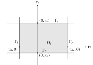
Consider a rectangular computational domain (ΩisubscriptΩ𝑖\Omega_{i}) with boundary segments parallel to one of the axes (see Fig. 1) with Ωi=(xl,xr)×(xb,xt)subscriptΩ𝑖subscript𝑥𝑙subscript𝑥𝑟subscript𝑥𝑏subscript𝑥𝑡\Omega_{i}=(x_{l},x_{r})\times(x_{b},x_{t}) referred to as the interior domain. Consider the decomposition of the field u(𝒙,t)𝑢𝒙𝑡u(\boldsymbol{x},t) such that u(𝒙,t)𝖫2(2)=𝖫2(Ωi)𝖫2(Ωe)𝑢𝒙𝑡superscript𝖫2superscript2direct-sumsuperscript𝖫2subscriptΩ𝑖superscript𝖫2subscriptΩ𝑒u(\boldsymbol{x},t)\in\mathsf{L}^{2}(\mathbb{R}^{2})=\mathsf{L}^{2}(\Omega_{i})\oplus\mathsf{L}^{2}(\Omega_{e}) where Ωe=2Ω¯isubscriptΩ𝑒superscript2subscript¯Ω𝑖\Omega_{e}=\mathbb{R}^{2}\setminus\overline{\Omega}_{i} is referred to as the exterior domain. An equivalent formulation of the IVP in (1) can be stated as
Refer to caption
Figure 1: The figure shows a rectangular domain with boundary segments parallel to one of the axes.
interior problem:{itv+v=0,(𝒙,t)Ωi×+,v(𝒙,0)=u0(𝒙),(𝒙,t)Ωi,exterior problem:{itw+w=0,(𝒙,t)Ωe×+,w(𝒙,0)=0,𝒙Ωe,lim|𝒙||𝒙|(w𝒙|𝒙|+eiπ4t1/2w)=0;continuity relations:v(𝒙,t)|Γ=w(𝒙,t)|Γ,nv(𝒙,t)|Γ=nw(𝒙,t)|Γ,\begin{split}\text{interior problem}:\quad&\left\{\begin{aligned} &i\partial_{t}v+\triangle v=0,\quad(\boldsymbol{x},t)\in\Omega_{i}\times\mathbb{R}_{+},\\ &v(\boldsymbol{x},0)=u_{0}(\boldsymbol{x}),\quad(\boldsymbol{x},t)\in\Omega_{i},\\ \end{aligned}\right.\\ \text{exterior problem}:\quad&\left\{\begin{aligned} &i\partial_{t}w+\triangle w=0,\quad(\boldsymbol{x},t)\in\Omega_{e}\times\mathbb{R}_{+},\\ &w(\boldsymbol{x},0)=0,\quad\boldsymbol{x}\in\Omega_{e},\\ &\lim_{|\boldsymbol{x}|\rightarrow\infty}\sqrt{|\boldsymbol{x}|}\left(\nabla w\cdot\frac{\boldsymbol{x}}{|\boldsymbol{x}|}+e^{-i\frac{\pi}{4}}\partial_{t}^{1/2}w\right)=0;\end{aligned}\right.\\ \text{continuity relations}:\quad&v(\boldsymbol{x},t)|_{\Gamma}=w(\boldsymbol{x},t)|_{\Gamma},\quad\partial_{n}v(\boldsymbol{x},t)|_{\Gamma}=\partial_{n}w(\boldsymbol{x},t)|_{\Gamma},\end{split} (2)

where ΓΓ\Gamma denotes the common boundary of the interior and the exterior domains. For the sake of completeness, we would like to present a detailed discussion of the derivation of the TBCs first presented in [5]. To this end, let (ζ1,ζ2)subscript𝜁1subscript𝜁2(\zeta_{1},\zeta_{2}) be the covariables corresponding to (x1,x2)subscript𝑥1subscript𝑥2(x_{1},x_{2}) to be used in the two dimensional Fourier transform. Let us denote the one dimensional Fourier transform of w(x1,x2,t)𝑤subscript𝑥1subscript𝑥2𝑡w(x_{1},x_{2},t) with respect to x2subscript𝑥2x_{2} by w~(x1,ζ2,t)~𝑤subscript𝑥1subscript𝜁2𝑡\widetilde{w}(x_{1},\zeta_{2},t):

w~(x1,ζ2,t)=x2[w(x1,x2,t)]w(x1,x2,t)eiζ2x2𝑑x2.~𝑤subscript𝑥1subscript𝜁2𝑡subscriptsubscript𝑥2delimited-[]𝑤subscript𝑥1subscript𝑥2𝑡subscript𝑤subscript𝑥1subscript𝑥2𝑡superscript𝑒𝑖subscript𝜁2subscript𝑥2differential-dsubscript𝑥2\begin{split}&\widetilde{w}(x_{1},\zeta_{2},t)=\mathscr{F}_{x_{2}}[w(x_{1},x_{2},t)]\equiv\int_{\mathbb{R}}w(x_{1},x_{2},t)e^{-i\zeta_{2}x_{2}}dx_{2}.\end{split}

Let us denote the Laplace transform of w~(x1,ζ2,t)~𝑤subscript𝑥1subscript𝜁2𝑡\widetilde{w}(x_{1},\zeta_{2},t) with respect to t𝑡t by W~(x1,ζ2,z)~𝑊subscript𝑥1subscript𝜁2𝑧\widetilde{W}(x_{1},\zeta_{2},z):

W~(x1,ζ2,t)=t[w~(x1,ζ2,t)]+w~(x1,ζ2,t)ezt𝑑t.~𝑊subscript𝑥1subscript𝜁2𝑡subscript𝑡delimited-[]~𝑤subscript𝑥1subscript𝜁2𝑡subscriptsubscript~𝑤subscript𝑥1subscript𝜁2𝑡superscript𝑒𝑧𝑡differential-d𝑡\begin{split}&\widetilde{W}(x_{1},\zeta_{2},t)=\mathscr{L}_{t}[\widetilde{w}(x_{1},\zeta_{2},t)]\equiv\int_{\mathbb{R}_{+}}\widetilde{w}(x_{1},\zeta_{2},t)e^{-zt}dt.\end{split}

First we focus on deriving the TBCs on the segment ΓrsubscriptΓ𝑟\Gamma_{r} by employing the Fourier transform with respect to x2subscript𝑥2x_{2} and then taking the Laplace transform of the right exterior problem:

(x12+α2)W~(x1,ζ2,z)=0,x1(xr,),formulae-sequencesuperscriptsubscriptsubscript𝑥12superscript𝛼2~𝑊subscript𝑥1subscript𝜁2𝑧0subscript𝑥1subscript𝑥𝑟(\partial_{x_{1}}^{2}+\alpha^{2})\widetilde{W}(x_{1},\zeta_{2},z)=0,\quad x_{1}\in(x_{r},\infty), (3)

where α=izζ22𝛼𝑖𝑧superscriptsubscript𝜁22\alpha=\sqrt{iz-\zeta_{2}^{2}} such that \sqrt{\cdot} denotes the branch with Im(α)>0Im𝛼0\operatorname{Im}(\alpha)>0. The solution takes the form

W~(x1,ζ2,z)=cexp(+iαx1)+dexp(iαx1),~𝑊subscript𝑥1subscript𝜁2𝑧𝑐𝑖𝛼subscript𝑥1𝑑𝑖𝛼subscript𝑥1\widetilde{W}({x}_{1},\zeta_{2},z)=c\exp(+i\alpha x_{1})+d\exp(-i\alpha x_{1}), (4)

where c𝑐c and d𝑑d are independent of x1subscript𝑥1x_{1}. In order to have a bounded solution on the right exterior domain, d𝑑d must be zero. Further, c𝑐c can be eliminated using the derivative of the field to obtain

x1W~(x1,ζ2,z)=iαW~(x1,ζ2,z).subscriptsubscript𝑥1~𝑊subscript𝑥1subscript𝜁2𝑧𝑖𝛼~𝑊subscript𝑥1subscript𝜁2𝑧\partial_{x_{1}}\widetilde{W}(x_{1},\zeta_{2},z)=i\alpha\widetilde{W}(x_{1},\zeta_{2},z). (5)

To facilitate the inverse Laplace transform of the equation above, we proceed as follows:

x1w~(x1,ζ2,t)=1[x1W~(x1,ζ2,z)]=1[iα1]1[α2W~(x1,ζ2,z)],subscriptsubscript𝑥1~𝑤subscript𝑥1subscript𝜁2𝑡superscript1delimited-[]subscriptsubscript𝑥1~𝑊subscript𝑥1subscript𝜁2𝑧superscript1delimited-[]𝑖superscript𝛼1superscript1delimited-[]superscript𝛼2~𝑊subscript𝑥1subscript𝜁2𝑧\partial_{x_{1}}\widetilde{w}(x_{1},\zeta_{2},t)=\mathscr{L}^{-1}[\partial_{x_{1}}\widetilde{W}(x_{1},\zeta_{2},z)]=\mathscr{L}^{-1}[i\alpha^{-1}]\star\mathscr{L}^{-1}[\alpha^{2}\widetilde{W}(x_{1},\zeta_{2},z)], (6)

where ‘\star’ represents the convolution operation with respect t𝑡t. Let us observe that 1[1/z](t)=H(t)/πtsuperscript1delimited-[]1𝑧𝑡𝐻𝑡𝜋𝑡\mathscr{L}^{-1}\left[{1}/{\sqrt{z}}\right](t)=H(t)/{\sqrt{\pi t}} where H(t)𝐻𝑡H(t) denotes the Heaviside step-function. In the following, we use the fractional operators which are denoted by tα,αsuperscriptsubscript𝑡𝛼𝛼\partial_{t}^{\alpha},\;\alpha\in\mathbb{R} (see Miller and Ross [20]). For α<0𝛼0\alpha<0, we obtain the Riemann-Liouville fractional integral of order |α|𝛼|\alpha| while α>0𝛼0\alpha>0 corresponds to fractional derivatives which are introduced as integral order derivatives of fractional integrals (discussed in A). Using the shifting property of Laplace transforms and introducing fractional operators of order 1/2121/2, we can express the result as

x1w~(x1,ζ2,t)=eiπ/4eiζ22tt1/2eiζ22t[itw~(x1,ζ2,t)ζ22w~(x1,ζ2,t)].subscriptsubscript𝑥1~𝑤subscript𝑥1subscript𝜁2𝑡superscript𝑒𝑖𝜋4superscript𝑒𝑖superscriptsubscript𝜁22𝑡superscriptsubscript𝑡12superscript𝑒𝑖superscriptsubscript𝜁22𝑡delimited-[]𝑖subscript𝑡~𝑤subscript𝑥1subscript𝜁2𝑡superscriptsubscript𝜁22~𝑤subscript𝑥1subscript𝜁2𝑡\partial_{x_{1}}\widetilde{w}(x_{1},\zeta_{2},t)=e^{i\pi/4}e^{-i\zeta_{2}^{2}t}\partial_{t}^{-1/2}e^{i\zeta_{2}^{2}t}\left[i\partial_{t}\widetilde{w}(x_{1},\zeta_{2},t)-\zeta_{2}^{2}\widetilde{w}(x_{1},\zeta_{2},t)\right]. (7)

In order to obtain the inverse Fourier transform of the above relations, let us introduce the kernel

𝒢(x2,t)=eiπ/44πtexp[ix224t],𝒢subscript𝑥2𝑡superscript𝑒𝑖𝜋44𝜋𝑡𝑖superscriptsubscript𝑥224𝑡\mathcal{G}(x_{2},t)=\frac{e^{-i\pi/4}}{\sqrt{4\pi t}}\exp\left[i\frac{x_{2}^{2}}{4t}\right], (8)

defined in a distributional sense with its Fourier transform given by G~(ζ2,t)=eiζ22t~𝐺subscript𝜁2𝑡superscript𝑒𝑖superscriptsubscript𝜁22𝑡\widetilde{G}(\zeta_{2},t)=e^{-i\zeta_{2}^{2}t}. Introducing the integral definition for 1/2121/2-order fractional integral and taking inverse Fourier transform of (7) yields

x1w(𝒙,t)=eiπ/4π0t[iτw(x1,x2,τ)+x22w(x1,x2,τ)]𝒢(x2x2,tτ)tτ𝑑x2𝑑τ.subscriptsubscript𝑥1𝑤𝒙𝑡superscript𝑒𝑖𝜋4𝜋superscriptsubscript0𝑡subscriptdelimited-[]𝑖subscript𝜏𝑤subscript𝑥1subscriptsuperscript𝑥2𝜏subscriptsuperscript2subscriptsuperscript𝑥2𝑤subscript𝑥1subscriptsuperscript𝑥2𝜏𝒢subscript𝑥2subscriptsuperscript𝑥2𝑡𝜏𝑡𝜏differential-dsuperscriptsubscript𝑥2differential-d𝜏\partial_{x_{1}}{w}(\boldsymbol{x},t)=\frac{e^{i\pi/4}}{\sqrt{\pi}}\int_{0}^{t}\int_{\mathbb{R}}\left[i\partial_{\tau}{w}(x_{1},x^{\prime}_{2},\tau)+\partial^{2}_{x^{\prime}_{2}}w(x_{1},x^{\prime}_{2},\tau)\right]\frac{\mathcal{G}(x_{2}-x^{\prime}_{2},t-\tau)}{\sqrt{t-\tau}}dx_{2}^{\prime}d\tau. (9)

The relationship above is referred to as the Dirichlet-to-Neumann (DtN) map relating the Dirichlet data w(x1,x2,t)𝑤subscript𝑥1subscript𝑥2𝑡{w}(x_{1},x_{2},t) to the Neumann data x1w(𝒙,t)subscriptsubscript𝑥1𝑤𝒙𝑡\partial_{x_{1}}w(\boldsymbol{x},t) on the right segment. Using the following result from calculus of fractional operators

t[eiζ22tt1/2eiζ22tw~(x1,ζ2,t)]=eiζ22tt1/2eiζ22ttw~(x1,ζ2,t),subscript𝑡delimited-[]superscript𝑒𝑖superscriptsubscript𝜁22𝑡superscriptsubscript𝑡12superscript𝑒𝑖superscriptsubscript𝜁22𝑡~𝑤subscript𝑥1subscript𝜁2𝑡superscript𝑒𝑖superscriptsubscript𝜁22𝑡superscriptsubscript𝑡12superscript𝑒𝑖superscriptsubscript𝜁22𝑡subscript𝑡~𝑤subscript𝑥1subscript𝜁2𝑡\partial_{t}\left[e^{-i\zeta_{2}^{2}t}\partial_{t}^{-1/2}e^{i\zeta_{2}^{2}t}\widetilde{w}(x_{1},\zeta_{2},t)\right]=e^{-i\zeta_{2}^{2}t}\partial_{t}^{-1/2}e^{i\zeta_{2}^{2}t}\partial_{t}\widetilde{w}(x_{1},\zeta_{2},t), (10)

we can recast (9) by taking out the operators from square bracketed term as

x1w(𝒙,t)=(tix22)eiπ/4π0tw(x1,x2,τ)𝒢(x2x2,tτ)tτ𝑑x2𝑑τ.subscriptsubscript𝑥1𝑤𝒙𝑡subscript𝑡𝑖subscriptsuperscript2subscript𝑥2superscript𝑒𝑖𝜋4𝜋superscriptsubscript0𝑡subscript𝑤subscript𝑥1subscriptsuperscript𝑥2𝜏𝒢subscript𝑥2subscriptsuperscript𝑥2𝑡𝜏𝑡𝜏differential-dsuperscriptsubscript𝑥2differential-d𝜏\partial_{x_{1}}{w}(\boldsymbol{x},t)=-(\partial_{t}-i\partial^{2}_{x_{2}})\frac{e^{-i\pi/4}}{\sqrt{\pi}}\int_{0}^{t}\int_{\mathbb{R}}w(x_{1},x^{\prime}_{2},\tau)\frac{\mathcal{G}(x_{2}-x^{\prime}_{2},t-\tau)}{\sqrt{t-\tau}}dx_{2}^{\prime}d\tau. (11)

In order to express the DtN map compactly, we introduce the notation

(tix22)1/2f(x2,t)=1π0tf(x2,τ)𝒢(x2x2,tτ)tτ𝑑x2𝑑τ.superscriptsubscript𝑡𝑖superscriptsubscriptsubscript𝑥2212𝑓subscript𝑥2𝑡1𝜋superscriptsubscript0𝑡subscript𝑓subscriptsuperscript𝑥2𝜏𝒢subscript𝑥2subscriptsuperscript𝑥2𝑡𝜏𝑡𝜏differential-dsuperscriptsubscript𝑥2differential-d𝜏(\partial_{t}-i\partial_{x_{2}}^{2})^{-1/2}f({x}_{2},t)\\ =\frac{1}{\sqrt{\pi}}\int_{0}^{t}\int_{\mathbb{R}}f(x^{\prime}_{2},\tau)\frac{\mathcal{G}(x_{2}-x^{\prime}_{2},t-\tau)}{\sqrt{t-\tau}}dx_{2}^{\prime}d\tau. (12)

so that

(tix22)[(tix22)1/2f]=(tix22)1/2f.subscript𝑡𝑖superscriptsubscriptsubscript𝑥22delimited-[]superscriptsubscript𝑡𝑖superscriptsubscriptsubscript𝑥2212𝑓superscriptsubscript𝑡𝑖superscriptsubscriptsubscript𝑥2212𝑓(\partial_{t}-i\partial_{x_{2}}^{2})[(\partial_{t}-i\partial_{x_{2}}^{2})^{-1/2}f]=(\partial_{t}-i\partial_{x_{2}}^{2})^{1/2}f.

Next, invoking the continuity relations defined in (2), the DtN map on the segment ΓrsubscriptΓ𝑟\Gamma_{r} can now be expressed in the compact form as

x1v(𝒙,t)+eiπ/4(tix22)1/2v(𝒙,t)=0.subscriptsubscript𝑥1𝑣𝒙𝑡superscript𝑒𝑖𝜋4superscriptsubscript𝑡𝑖subscriptsuperscript2subscript𝑥212𝑣𝒙𝑡0\partial_{x_{1}}{v}(\boldsymbol{x},t)+e^{-i\pi/4}(\partial_{t}-i\partial^{2}_{x_{2}})^{1/2}v(\boldsymbol{x},t)=0. (13)

One can obtain the transparent boundary conditions for the rest of the boundary segments of the domain ΩisubscriptΩ𝑖\Omega_{i} in a similar fashion which yields the following equivalent formulation of the IVP corresponding to (1) on the computational domain ΩisubscriptΩ𝑖\Omega_{i}:

{itu+u=0,(𝒙,t)Ωi×+,u(𝒙,0)=u0(𝒙)𝖫2(Ωi),suppu0Ωi,nu+eiπ/4(tix22)1/2u=0,𝒙ΓlΓr,t>0,nu+eiπ/4(tix12)1/2u=0,𝒙ΓbΓt,t>0.\left\{\begin{aligned} &i\partial_{t}u+\triangle u=0,\quad(\boldsymbol{x},t)\in\Omega_{i}\times\mathbb{R}_{+},\\ &u(\boldsymbol{x},0)=u_{0}(\boldsymbol{x})\in\mathsf{L}^{2}(\Omega_{i}),\quad\operatorname*{supp}\,u_{0}\subset\Omega_{i},\\ &\partial_{n}{u}+e^{-i\pi/4}(\partial_{t}-i\partial^{2}_{x_{2}})^{1/2}u=0,\quad\boldsymbol{x}\in\Gamma_{l}\cup\Gamma_{r},\,t>0,\\ &\partial_{n}{u}+e^{-i\pi/4}(\partial_{t}-i\partial^{2}_{x_{1}})^{1/2}u=0,\quad\boldsymbol{x}\in\Gamma_{b}\cup\Gamma_{t},\,t>0.\end{aligned}\right. (14)

Note that the operators present in the DtN maps are non-local both in space and time. For the numerical solution of this IBVP, a suitable numerical implementation needs to be developed. Before we address the numerical aspects, we develop a suitable representation for these operators at the continuous level that is compatible with the rectangular domain. The earliest approach was due to Menza [7] which is discussed in Sec. 2.3. This approach is based on Padé approximant for the square root function, however, the treatment at the corners is inexact. A more recent approach was presented by Feshchenko and Popov [4] who developed a representation in terms of fractional operators. We discuss this approach in Sec. 2.1 where we adopt a more direct way to arrive at the results as presented by the second author [5]. Finally, we present one of the main contributions of this paper in Sec. 2.2 where a novel Padé based approach is described that is capable of handling the corners of the domain in a natural manner.

2.1 Fractional operator based approach

In this section, we focus on expressing the DtN maps in terms of (time-)fractional operators. To this end, let us recall the form of the DtN map given by (7) in terms of the Fourier variables so that

x1w~(x1,ζ2,t)=eiπ/4eiζ22tt1/2eiζ22t[itw~(x1,ζ2,t)ζ22w~(x1,ζ2,t)]=ieiπ/4eiζ22tt1/2eiζ22tw~(x1,ζ2,t)=eiπ/4t1/2eiζ22(tt)w~(x1,ζ2,t)|t=t.subscriptsubscript𝑥1~𝑤subscript𝑥1subscript𝜁2𝑡superscript𝑒𝑖𝜋4superscript𝑒𝑖superscriptsubscript𝜁22𝑡superscriptsubscript𝑡12superscript𝑒𝑖superscriptsubscript𝜁22𝑡delimited-[]𝑖subscript𝑡~𝑤subscript𝑥1subscript𝜁2𝑡superscriptsubscript𝜁22~𝑤subscript𝑥1subscript𝜁2𝑡𝑖superscript𝑒𝑖𝜋4superscript𝑒𝑖superscriptsubscript𝜁22𝑡superscriptsubscript𝑡12superscript𝑒𝑖superscriptsubscript𝜁22𝑡~𝑤subscript𝑥1subscript𝜁2𝑡evaluated-atsuperscript𝑒𝑖𝜋4superscriptsubscriptsuperscript𝑡12superscript𝑒𝑖superscriptsubscript𝜁22𝑡superscript𝑡~𝑤subscript𝑥1subscript𝜁2superscript𝑡superscript𝑡𝑡\begin{split}\partial_{x_{1}}\widetilde{w}(x_{1},\zeta_{2},t)&=e^{i\pi/4}e^{-i\zeta_{2}^{2}t}\partial_{t}^{-1/2}e^{i\zeta_{2}^{2}t}\left[i\partial_{t}\widetilde{w}(x_{1},\zeta_{2},t)-\zeta_{2}^{2}\widetilde{w}(x_{1},\zeta_{2},t)\right]=ie^{i\pi/4}e^{-i\zeta_{2}^{2}t}\partial_{t}^{1/2}e^{i\zeta_{2}^{2}t}\widetilde{w}(x_{1},\zeta_{2},t)\\ &=-e^{-i\pi/4}\partial_{t^{\prime}}^{1/2}e^{-i\zeta_{2}^{2}(t-t^{\prime})}\left.\widetilde{w}(x_{1},\zeta_{2},t^{\prime})\right|_{t^{\prime}=t}.\end{split} (15)

where the last step uses the composition rule for fractional operators. Introducing the auxiliary function φ(x1,x2,τ1,τ2)𝜑subscript𝑥1subscript𝑥2subscript𝜏1subscript𝜏2\varphi(x_{1},x_{2},\tau_{1},\tau_{2}) such that

x2[φ](x1,x2,τ1,τ2)=eiζ22(τ2τ1)w~(x1,ζ2,τ1),subscriptsubscript𝑥2delimited-[]𝜑subscript𝑥1subscript𝑥2subscript𝜏1subscript𝜏2superscript𝑒𝑖superscriptsubscript𝜁22subscript𝜏2subscript𝜏1~𝑤subscript𝑥1subscript𝜁2subscript𝜏1\mathscr{F}_{x_{2}}[\varphi](x_{1},x_{2},\tau_{1},\tau_{2})=e^{-i\zeta_{2}^{2}(\tau_{2}-\tau_{1})}\widetilde{w}(x_{1},\zeta_{2},\tau_{1}), (16)

we can express the DtN map on the segment ΓrsubscriptΓ𝑟\Gamma_{r} as:

x1w(x1,x2,t)=eiπ/4τ11/2φ(x1,x2,τ1,τ2)|τ1=τ2=t.subscriptsubscript𝑥1𝑤subscript𝑥1subscript𝑥2𝑡evaluated-atsuperscript𝑒𝑖𝜋4superscriptsubscriptsubscript𝜏112𝜑subscript𝑥1subscript𝑥2subscript𝜏1subscript𝜏2subscript𝜏1subscript𝜏2𝑡\partial_{x_{1}}w(x_{1},x_{2},t)=-\left.e^{-i\pi/4}\partial_{\tau_{1}}^{1/2}\varphi(x_{1},x_{2},\tau_{1},\tau_{2})\right|_{\tau_{1}=\tau_{2}=t}. (17)

Numerical implementation of this fractional derivative requires the history of the auxiliary function from the start of the computations. This can be facilitated by the IVP satisfied by φ(x1,x2,τ1,τ2)𝜑subscript𝑥1subscript𝑥2subscript𝜏1subscript𝜏2\varphi(x_{1},x_{2},\tau_{1},\tau_{2}) which follows from the definition (16):

[iτ2+x22]φ(x1,x2,τ1,τ2)=0,τ2(τ1,t],x1=xr,formulae-sequencedelimited-[]𝑖subscriptsubscript𝜏2subscriptsuperscript2subscript𝑥2𝜑subscript𝑥1subscript𝑥2subscript𝜏1subscript𝜏20formulae-sequencesubscript𝜏2subscript𝜏1𝑡subscript𝑥1subscript𝑥𝑟[i\partial_{\tau_{2}}+\partial^{2}_{x_{2}}]\varphi(x_{1},x_{2},\tau_{1},\tau_{2})=0,\quad\tau_{2}\in(\tau_{1},t],\quad x_{1}=x_{r}, (18)

where the diagonal values φ(x1,x2,τ1,τ1)=w(x1,x2,τ1)𝜑subscript𝑥1subscript𝑥2subscript𝜏1subscript𝜏1𝑤subscript𝑥1subscript𝑥2subscript𝜏1\varphi(x_{1},x_{2},\tau_{1},\tau_{1})=w(x_{1},x_{2},\tau_{1}) serve as the initial condition. Note that the history is needed for all τ1[0,t]subscript𝜏10𝑡\tau_{1}\in[0,t] which means that we must solve the IVP for all τ1[0,t]subscript𝜏10𝑡\tau_{1}\in[0,t] over ΓrsubscriptΓ𝑟\Gamma_{r}. It is interesting to note that the IVP satisfied by the auxiliary function on the segment ΓrsubscriptΓ𝑟\Gamma_{r} turns out to be a one-dimensional Schrödinger equation. The exact boundary conditions are well-known for this equation when the initial data is compactly supported. The formulation of the TBCs for the IVP (18) requires us to first understand the support (with respect to x2subscript𝑥2x_{2}) of the auxiliary function on the segment ΓrsubscriptΓ𝑟\Gamma_{r} at τ2=0subscript𝜏20\tau_{2}=0. From the knowledge of the compact support of the initial field u0(𝒙)subscript𝑢0𝒙u_{0}(\boldsymbol{x}), we can establish the support of the auxiliary function at τ2=0subscript𝜏20\tau_{2}=0. Let u~0(𝜻)=(x1,x2)u0(𝒙)subscript~𝑢0𝜻subscriptsubscript𝑥1subscript𝑥2subscript𝑢0𝒙\widetilde{u}_{0}(\boldsymbol{\zeta})=\mathscr{F}_{(x_{1},x_{2})}u_{0}(\boldsymbol{x}), then taking the Fourier transform of the IVP defined by (1), we obtain

tu~(𝜻)+i(ζ12+ζ22)u~(𝜻)=0.subscript𝑡~𝑢𝜻𝑖superscriptsubscript𝜁12superscriptsubscript𝜁22~𝑢𝜻0\partial_{t}\widetilde{u}(\boldsymbol{\zeta})+i(\zeta_{1}^{2}+\zeta_{2}^{2})\widetilde{u}(\boldsymbol{\zeta})=0. (19)

Taking into account the initial condition, the solution to this IVP becomes u~(𝜻,t)=ei(ζ12+ζ22)tu~0(𝜻)~𝑢𝜻𝑡superscript𝑒𝑖superscriptsubscript𝜁12superscriptsubscript𝜁22𝑡subscript~𝑢0𝜻\widetilde{u}(\boldsymbol{\zeta},t)=e^{-i(\zeta_{1}^{2}+\zeta_{2}^{2})t}\widetilde{u}_{0}(\boldsymbol{\zeta}) which yields

x1,x2[φ](x1,x2,τ1,τ2)=eiζ22(τ2τ1)u~(ζ1,ζ2,τ1)=eiζ22(τ2τ1)ei(ζ12+ζ22)τ1u~0(𝜻),φ(x1,x2,τ1,τ2)=1(2π)22ei𝜻𝒙iζ12τ1iζ22τ2u~0(𝜻)d2𝜻.formulae-sequencesubscriptsubscript𝑥1subscript𝑥2delimited-[]𝜑subscript𝑥1subscript𝑥2subscript𝜏1subscript𝜏2superscript𝑒𝑖superscriptsubscript𝜁22subscript𝜏2subscript𝜏1~𝑢subscript𝜁1subscript𝜁2subscript𝜏1superscript𝑒𝑖superscriptsubscript𝜁22subscript𝜏2subscript𝜏1superscript𝑒𝑖superscriptsubscript𝜁12superscriptsubscript𝜁22subscript𝜏1subscript~𝑢0𝜻𝜑subscript𝑥1subscript𝑥2subscript𝜏1subscript𝜏21superscript2𝜋2subscriptsuperscript2superscript𝑒𝑖𝜻𝒙𝑖superscriptsubscript𝜁12subscript𝜏1𝑖superscriptsubscript𝜁22subscript𝜏2subscript~𝑢0𝜻superscript𝑑2𝜻\begin{split}&\mathscr{F}_{x_{1},x_{2}}[\varphi](x_{1},x_{2},\tau_{1},\tau_{2})=e^{-i\zeta_{2}^{2}(\tau_{2}-\tau_{1})}\widetilde{u}(\zeta_{1},\zeta_{2},\tau_{1})=e^{-i\zeta_{2}^{2}(\tau_{2}-\tau_{1})}e^{-i(\zeta_{1}^{2}+\zeta_{2}^{2})\tau_{1}}\widetilde{u}_{0}(\boldsymbol{\zeta}),\\ &\varphi(x_{1},x_{2},\tau_{1},\tau_{2})=\frac{1}{(2\pi)^{2}}\int_{\mathbb{R}^{2}}e^{i\boldsymbol{\zeta}\cdot\boldsymbol{x}-i\zeta_{1}^{2}\tau_{1}-i\zeta_{2}^{2}\tau_{2}}\widetilde{u}_{0}(\boldsymbol{\zeta})d^{2}\boldsymbol{\zeta}.\end{split} (20)

From the definition of the auxiliary function written above as inverse Fourier transform consisting of u~0(𝜻)subscript~𝑢0𝜻\widetilde{u}_{0}(\boldsymbol{\zeta}), we can establish that the suppx2φ(xr,x2,τ1,0)[xb,xt]subscriptsuppsubscript𝑥2𝜑subscript𝑥𝑟subscript𝑥2subscript𝜏10subscript𝑥𝑏subscript𝑥𝑡\operatorname*{supp}_{x_{2}}\varphi(x_{r},x_{2},\tau_{1},0)\subset[x_{b},x_{t}] by considering the support of the initial field at τ2=0subscript𝜏20\tau_{2}=0. It is straightforward to see that the auxiliary function also satisfies the IVP

[iτ1+x12]φ(x1,x2,τ1,τ2)=0,τ1(τ2,t],formulae-sequencedelimited-[]𝑖subscriptsubscript𝜏1subscriptsuperscript2subscript𝑥1𝜑subscript𝑥1subscript𝑥2subscript𝜏1subscript𝜏20subscript𝜏1subscript𝜏2𝑡[i\partial_{\tau_{1}}+\partial^{2}_{x_{1}}]\varphi(x_{1},x_{2},\tau_{1},\tau_{2})=0,\quad\tau_{1}\in(\tau_{2},t], (21)

where diagonal values φ(x1,x2,τ2,τ2)=w(x1,x2,τ2)𝜑subscript𝑥1subscript𝑥2subscript𝜏2subscript𝜏2𝑤subscript𝑥1subscript𝑥2subscript𝜏2\varphi(x_{1},x_{2},\tau_{2},\tau_{2})=w(x_{1},x_{2},\tau_{2}) serves as the initial condition. Note that we solve the IVP for all τ2[0,t]subscript𝜏20𝑡\tau_{2}\in[0,t]. The transparent boundary condition at the end points of the segment ΓrsubscriptΓ𝑟\Gamma_{r} becomes:

x2φ(x1,x2,τ1,τ2)±eiπ/4τ21/2φ(x1,x2,τ1,τ2)=0,plus-or-minussubscriptsubscript𝑥2𝜑subscript𝑥1subscript𝑥2subscript𝜏1subscript𝜏2superscript𝑒𝑖𝜋4subscriptsuperscript12subscript𝜏2𝜑subscript𝑥1subscript𝑥2subscript𝜏1subscript𝜏20\partial_{x_{2}}\varphi(x_{1},x_{2},\tau_{1},\tau_{2})\pm e^{-i\pi/4}\partial^{1/2}_{\tau_{2}}\varphi(x_{1},x_{2},\tau_{1},\tau_{2})=0, (22)

where the sign is determined by x2{xt,xb}subscript𝑥2subscript𝑥𝑡subscript𝑥𝑏x_{2}\in\{x_{t},x_{b}\}, respectively. Note that the fractional derivative (τ21/2superscriptsubscriptsubscript𝜏212\partial_{\tau_{2}}^{1/2}) requires the knowledge of φ(x1,x2,τ1,τ2)𝜑subscript𝑥1subscript𝑥2subscript𝜏1subscript𝜏2\varphi(x_{1},x_{2},\tau_{1},\tau_{2}) at the end points of ΓrsubscriptΓ𝑟\Gamma_{r} from the start of the computation. The DtN map in terms of a time-fractional derivative operator for the IVP (14) can be expressed as

x1u(𝒙,t)=eiπ/4τ11/2φ(x1,x2,τ1,τ2)|τ1,τ2=t,(x1,x2)Γr,x1u(𝒙,t)=+eiπ/4τ11/2φ(x1,x2,τ1,τ2)|τ1,τ2=t,(x1,x2)Γl,x2u(𝒙,t)=eiπ/4τ21/2φ(x1,x2,τ1,τ2)|τ1,τ2=t,(x1,x2)Γt,x2u(𝒙,t)=+eiπ/4τ21/2φ(x1,x2,τ1,τ2)|τ1,τ2=t,(x1,x2)Γb.\begin{split}&\partial_{x_{1}}{u}(\boldsymbol{x},t)=\left.-{e^{-i\pi/4}}\partial^{1/2}_{\tau_{1}}\varphi(x_{1},x_{2},\tau_{1},\tau_{2})\right|_{\tau_{1},\tau_{2}=t},\quad(x_{1},x_{2})\in\Gamma_{r},\\ &\partial_{x_{1}}{u}(\boldsymbol{x},t)=\left.+{e^{-i\pi/4}}\partial^{1/2}_{\tau_{1}}\varphi(x_{1},x_{2},\tau_{1},\tau_{2})\right|_{\tau_{1},\tau_{2}=t},\quad(x_{1},x_{2})\in\Gamma_{l},\\ &\partial_{x_{2}}{u}(\boldsymbol{x},t)=\left.-{e^{-i\pi/4}}\partial^{1/2}_{\tau_{2}}\varphi(x_{1},x_{2},\tau_{1},\tau_{2})\right|_{\tau_{1},\tau_{2}=t},\quad(x_{1},x_{2})\in\Gamma_{t},\\ &\partial_{x_{2}}{u}(\boldsymbol{x},t)=\left.+{e^{-i\pi/4}}\partial^{1/2}_{\tau_{2}}\varphi(x_{1},x_{2},\tau_{1},\tau_{2})\right|_{\tau_{1},\tau_{2}=t},\quad(x_{1},x_{2})\in\Gamma_{b}.\end{split} (23)

The IVPs for the auxiliary function are summarised below

[iτ1+x12]φ(x1,x2,τ1,τ2)=0,(x1,x2)ΓtΓb,τ1(τ2,t],[iτ2+x22]φ(x1,x2,τ1,τ2)=0,(x1,x2)ΓlΓr,τ2(τ1,t].\begin{split}&[i\partial_{\tau_{1}}+\partial_{x_{1}}^{2}]\varphi(x_{1},x_{2},\tau_{1},\tau_{2})=0,\quad(x_{1},x_{2})\in\Gamma_{t}\cup\Gamma_{b},\;\tau_{1}\in(\tau_{2},t],\\ &[i\partial_{\tau_{2}}+\partial_{x_{2}}^{2}]\varphi(x_{1},x_{2},\tau_{1},\tau_{2})=0,\quad(x_{1},x_{2})\in\Gamma_{l}\cup\Gamma_{r},\;\tau_{2}\in(\tau_{1},t].\end{split} (24)

Let us introduce the set of corner points of the computational domain as {Γrt,Γrb,Γlt,Γlb}subscriptΓ𝑟𝑡subscriptΓ𝑟𝑏subscriptΓ𝑙𝑡subscriptΓ𝑙𝑏\{\Gamma_{rt},\Gamma_{rb},\Gamma_{lt},\Gamma_{lb}\} where Γij=ΓiΓjsubscriptΓ𝑖𝑗subscriptΓ𝑖subscriptΓ𝑗\Gamma_{ij}=\Gamma_{i}\cap\Gamma_{j} with i,j{r,t,l,b}𝑖𝑗𝑟𝑡𝑙𝑏i,j\in\{r,t,l,b\}. The transparent boundary conditions at corner points for the IVPs listed in (24) are as follows

x1φ(x1,x2,τ1,τ2)+eiπ/4τ11/2φ(x1,x2,τ1,τ2)=0,(x1,x2){Γrt,Γrb},x1φ(x1,x2,τ1,τ2)eiπ/4τ11/2φ(x1,x2,τ1,τ2)=0,(x1,x2){Γlt,Γlb},x2φ(x1,x2,τ1,τ2)+eiπ/4τ21/2φ(x1,x2,τ1,τ2)=0,(x1,x2){Γrt,Γlt},x2φ(x1,x2,τ1,τ2)eiπ/4τ21/2φ(x1,x2,τ1,τ2)=0.(x1,x2){Γrb,Γlb},\begin{split}&\partial_{x_{1}}\varphi(x_{1},x_{2},\tau_{1},\tau_{2})+e^{-i\pi/4}\partial^{1/2}_{\tau_{1}}\varphi(x_{1},x_{2},\tau_{1},\tau_{2})=0,\quad(x_{1},x_{2})\in\{\Gamma_{rt},\Gamma_{rb}\},\\ &\partial_{x_{1}}\varphi(x_{1},x_{2},\tau_{1},\tau_{2})-e^{-i\pi/4}\partial^{1/2}_{\tau_{1}}\varphi(x_{1},x_{2},\tau_{1},\tau_{2})=0,\quad(x_{1},x_{2})\in\{\Gamma_{lt},\Gamma_{lb}\},\\ &\partial_{x_{2}}\varphi(x_{1},x_{2},\tau_{1},\tau_{2})+e^{-i\pi/4}\partial^{1/2}_{\tau_{2}}\varphi(x_{1},x_{2},\tau_{1},\tau_{2})=0,\quad(x_{1},x_{2})\in\{\Gamma_{rt},\Gamma_{lt}\},\\ &\partial_{x_{2}}\varphi(x_{1},x_{2},\tau_{1},\tau_{2})-e^{-i\pi/4}\partial^{1/2}_{\tau_{2}}\varphi(x_{1},x_{2},\tau_{1},\tau_{2})=0.\quad(x_{1},x_{2})\in\{\Gamma_{rb},\Gamma_{lb}\},\\ \end{split} (25)

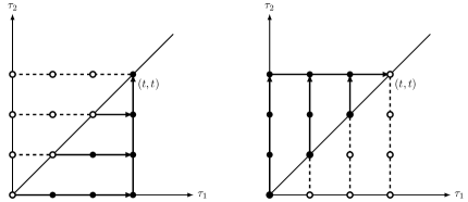
The history required for the fractional derivatives present in the DtN maps can be understood with the help of the schematic shown in Fig. 2. The two IVPs for the auxiliary field φ(x1,x2,τ1,τ2)𝜑subscript𝑥1subscript𝑥2subscript𝜏1subscript𝜏2\varphi(x_{1},x_{2},\tau_{1},\tau_{2}) advances the field either above or below the diagonal in the (τ1,τ2)subscript𝜏1subscript𝜏2(\tau_{1},\tau_{2})-plane starting from the diagonal which also serves as initial conditions for solving IVPs. This is depicted by filled circles where arrows denote the direction of evolution. The TBCs present in (25) to solve the IVPs for the auxiliary functions on the boundary segments require the history of the auxiliary function at corners from the start of the computations which makes the empty circles relevant. Note that these values at the corners can be taken from the adjacent segment of the boundary where it is already being computed. This is depicted by broken lines in Fig. 2.
Refer to caption
Figure 2: A schematic depiction of the evolution of the auxiliary field φ(x1,x2,τ1,τ2)𝜑subscript𝑥1subscript𝑥2subscript𝜏1subscript𝜏2\varphi(x_{1},x_{2},\tau_{1},\tau_{2}) in the (τ1,τ2)subscript𝜏1subscript𝜏2(\tau_{1},\tau_{2})-plane is provided in this figure where the plot on the right corresponds 𝒙ΓrΓl𝒙subscriptΓ𝑟subscriptΓ𝑙\boldsymbol{x}\in\Gamma_{r}\cup\Gamma_{l} and the plot on the left corresponds 𝒙ΓtΓb𝒙subscriptΓ𝑡subscriptΓ𝑏\boldsymbol{x}\in\Gamma_{t}\cup\Gamma_{b}. The filled circles depict the evolution of the auxiliary field φ(x1,x2,τ1,τ2)𝜑subscript𝑥1subscript𝑥2subscript𝜏1subscript𝜏2\varphi(x_{1},x_{2},\tau_{1},\tau_{2}) either above or below the diagonal in the (τ1,τ2)subscript𝜏1subscript𝜏2(\tau_{1},\tau_{2})-plane starting from the diagonal which also serves as initial conditions for solving IVPs corresponding to the auxiliary function. The TBCs for the auxiliary field require the history of the auxiliary field at the corner points which makes empty circles relevant. Note that these values at the corners can be taken from the adjacent segment of the boundary where it is already being computed and this is depicted by broken lines. Note that the vertical/horizontal lines where the arrows end corresponds to the history of the auxiliary field needed for the TBCs on ΩisubscriptΩ𝑖\partial\Omega_{i} in the current time (t𝑡t).

2.1.1 Corner conditions

Having discussed the boundary conditions satisfied by the field on the four segments of the computational domain (ΩisubscriptΩ𝑖\Omega_{i}) as stated in (23), we turn to the constraints on the field at the corners ({Γrt,Γrb,Γlt,Γlb}subscriptΓ𝑟𝑡subscriptΓ𝑟𝑏subscriptΓ𝑙𝑡subscriptΓ𝑙𝑏\{\Gamma_{rt},\Gamma_{rb},\Gamma_{lt},\Gamma_{lb}\}) which will be used later for solving the IBVP in (14) with a Galerkin method. Let us understand this by considering the corner ΓrtsubscriptΓ𝑟𝑡\Gamma_{rt} and recall the DtN map over segment ΓrsubscriptΓ𝑟\Gamma_{r} from (23)

x1u(x1,x2,t)=eiπ/4τ11/2φ(x1,x2,τ1,τ2)|τ1=τ2=t.subscriptsubscript𝑥1𝑢subscript𝑥1subscript𝑥2𝑡evaluated-atsuperscript𝑒𝑖𝜋4subscriptsuperscript12subscript𝜏1𝜑subscript𝑥1subscript𝑥2subscript𝜏1subscript𝜏2subscript𝜏1subscript𝜏2𝑡\partial_{x_{1}}{u}(x_{1},x_{2},t)=\left.-{e^{-i\pi/4}}\partial^{1/2}_{\tau_{1}}\varphi(x_{1},x_{2},\tau_{1},\tau_{2})\right|_{\tau_{1}=\tau_{2}=t}.

Applying x2subscriptsubscript𝑥2\partial_{x_{2}} to obtain the additional constraints on the field at corners, we have

x2x1u(x1,x2,t)=eiπ/4τ11/2x2φ(x1,x2,τ1,τ2)|τ1=τ2=t.subscriptsubscript𝑥2subscriptsubscript𝑥1𝑢subscript𝑥1subscript𝑥2𝑡evaluated-atsuperscript𝑒𝑖𝜋4subscriptsuperscript12subscript𝜏1subscriptsubscript𝑥2𝜑subscript𝑥1subscript𝑥2subscript𝜏1subscript𝜏2subscript𝜏1subscript𝜏2𝑡\partial_{x_{2}}\partial_{x_{1}}{u}(x_{1},x_{2},t)=\left.-{e^{-i\pi/4}}\partial^{1/2}_{\tau_{1}}\partial_{x_{2}}\varphi(x_{1},x_{2},\tau_{1},\tau_{2})\right|_{\tau_{1}=\tau_{2}=t}.

Now, plugging-in the value of x2φ(x1,x2,τ1,τ2)subscriptsubscript𝑥2𝜑subscript𝑥1subscript𝑥2subscript𝜏1subscript𝜏2\partial_{x_{2}}\varphi(x_{1},x_{2},\tau_{1},\tau_{2}) from (25) at the corner point ΓrtsubscriptΓ𝑟𝑡\Gamma_{rt}, we obtain the following corner condition

x1x2u(x1,x2,t)=eiπ/4eiπ/4τ11/2τ21/2φ(x1,x2,τ1,τ2)|τ1=τ2=t.subscriptsubscript𝑥1subscriptsubscript𝑥2𝑢subscript𝑥1subscript𝑥2𝑡evaluated-atsuperscript𝑒𝑖𝜋4superscript𝑒𝑖𝜋4subscriptsuperscript12subscript𝜏1subscriptsuperscript12subscript𝜏2𝜑subscript𝑥1subscript𝑥2subscript𝜏1subscript𝜏2subscript𝜏1subscript𝜏2𝑡\partial_{x_{1}}\partial_{x_{2}}{u}(x_{1},x_{2},t)=\left.e^{-i\pi/4}{e^{-i\pi/4}}\partial^{1/2}_{\tau_{1}}\partial^{1/2}_{\tau_{2}}\varphi(x_{1},x_{2},\tau_{1},\tau_{2})\right|_{\tau_{1}=\tau_{2}=t}. (26)

2.2 Novel-Padé based approach

In this section, we would like to explore the Padé approximant based representation for the 1/2121/2-order temporal derivative in (23) and its other ramifications. It is well-known that a rational approximation to the square-root function would allow one to obtain an effectively local approximation for the fractional derivative operator. We contrast this with the situation where the history grows with each time-step making it expensive computationally as well as from a storage point of view.

The diagonal Padé approximants for 1z1𝑧\sqrt{1-z}, with negative real axis as the branch-cut, can be used to obtain rational approximation RM(z)subscript𝑅𝑀𝑧R_{M}(z) for the function z𝑧\sqrt{z} as

RM(z)=b0k=1Mbkz+ηk2,where{b0=2M+1,bk=2ηk2(1+ηk2)2M+1,ηk=tanθk,θk=kπ2M+1,k=1,2,,M.R_{M}(z)=b_{0}-\sum_{k=1}^{M}\frac{b_{k}}{z+\eta^{2}_{k}},\quad\text{where}\quad\left\{\begin{aligned} &b_{0}=2M+1,\;b_{k}=\frac{2\eta^{2}_{k}(1+\eta^{2}_{k})}{2M+1},\\ &\eta_{k}=\tan\theta_{k},\;\theta_{k}=\frac{k\pi}{2M+1},\;k=1,2,\ldots,M.\end{aligned}\right. (27)

Here, the expression for the diagonal Padé approximant is taken from [21]. Let us start by introducing some compact notations for the auxiliary functions as:

φa1(x2,τ1,τ2)=φ(xa1,x2,τ1,τ2),a1{l,r},φa2(x1,τ1,τ2)=φ(x1,xa2,τ1,τ2),a2{b,t}.\begin{split}&\varphi_{a_{1}}(x_{2},\tau_{1},\tau_{2})=\varphi(x_{a_{1}},x_{2},\tau_{1},\tau_{2}),\quad a_{1}\in\{l,r\},\\ &\varphi_{a_{2}}(x_{1},\tau_{1},\tau_{2})=\varphi(x_{1},x_{a_{2}},\tau_{1},\tau_{2}),\quad a_{2}\in\{b,t\}.\end{split} (28)

Let z𝑧z\in\mathbb{C}, then the Laplace transform of the auxiliary function can be denoted as

τ1[φa1(x2,τ1,τ2)]=Φa1(x2,z,τ2),τ2[φa2(x1,τ1,τ2)]=Φa2(x1,τ1,z).formulae-sequencesubscriptsubscript𝜏1delimited-[]subscript𝜑subscript𝑎1subscript𝑥2subscript𝜏1subscript𝜏2subscriptΦsubscript𝑎1subscript𝑥2𝑧subscript𝜏2subscriptsubscript𝜏2delimited-[]subscript𝜑subscript𝑎2subscript𝑥1subscript𝜏1subscript𝜏2subscriptΦsubscript𝑎2subscript𝑥1subscript𝜏1𝑧\mathscr{L}_{\tau_{1}}[\varphi_{a_{1}}(x_{2},\tau_{1},\tau_{2})]=\varPhi_{a_{1}}(x_{2},z,\tau_{2}),\quad\mathscr{L}_{\tau_{2}}[\varphi_{a_{2}}(x_{1},\tau_{1},\tau_{2})]=\varPhi_{a_{2}}(x_{1},\tau_{1},z). (29)

The DtN maps described in (23) on the segments Γa1subscriptΓsubscript𝑎1\Gamma_{a_{1}} and Γa2subscriptΓsubscript𝑎2\Gamma_{a_{2}} can be restated as

x1u(x1,x2,t)±eiπ/4z1[zΦa1(x2,z,τ2)]|τ1=τ2=t=0,x2u(x1,x2,t)±eiπ/4z1[zΦa2(x2,τ1,z)]|τ1=τ2=t=0.formulae-sequenceplus-or-minussubscriptsubscript𝑥1𝑢subscript𝑥1subscript𝑥2𝑡evaluated-atsuperscript𝑒𝑖𝜋4subscriptsuperscript1𝑧delimited-[]𝑧subscriptΦsubscript𝑎1subscript𝑥2𝑧subscript𝜏2subscript𝜏1subscript𝜏2𝑡0plus-or-minussubscriptsubscript𝑥2𝑢subscript𝑥1subscript𝑥2𝑡evaluated-atsuperscript𝑒𝑖𝜋4subscriptsuperscript1𝑧delimited-[]𝑧subscriptΦsubscript𝑎2subscript𝑥2subscript𝜏1𝑧subscript𝜏1subscript𝜏2𝑡0\begin{split}&\partial_{x_{1}}{u}(x_{1},x_{2},t)\pm e^{-i\pi/4}\left.\mathscr{L}^{-1}_{z}\left[\sqrt{z}\varPhi_{a_{1}}(x_{2},z,\tau_{2})\right]\right|_{\tau_{1}=\tau_{2}=t}=0,\\ &\partial_{x_{2}}{u}(x_{1},x_{2},t)\pm e^{-i\pi/4}\left.\mathscr{L}^{-1}_{z}\left[\sqrt{z}\varPhi_{a_{2}}(x_{2},\tau_{1},z)\right]\right|_{\tau_{1}=\tau_{2}=t}=0.\end{split} (30)

Inserting the rational approximation of order M𝑀M for the function z𝑧\sqrt{z} as

x1u(x1,x2,t)±eiπ/4z1[RM(z)Φa1(x2,z,τ2)]|τ1=τ2=t0,x2u(x1,x2,t)±eiπ/4z1[RM(z)Φa2(x2,τ1,z)]|τ1=τ2=t0.formulae-sequenceplus-or-minussubscriptsubscript𝑥1𝑢subscript𝑥1subscript𝑥2𝑡evaluated-atsuperscript𝑒𝑖𝜋4subscriptsuperscript1𝑧delimited-[]subscript𝑅𝑀𝑧subscriptΦsubscript𝑎1subscript𝑥2𝑧subscript𝜏2subscript𝜏1subscript𝜏2𝑡0plus-or-minussubscriptsubscript𝑥2𝑢subscript𝑥1subscript𝑥2𝑡evaluated-atsuperscript𝑒𝑖𝜋4subscriptsuperscript1𝑧delimited-[]subscript𝑅𝑀𝑧subscriptΦsubscript𝑎2subscript𝑥2subscript𝜏1𝑧subscript𝜏1subscript𝜏2𝑡0\begin{split}&\partial_{x_{1}}{u}(x_{1},x_{2},t)\pm e^{-i\pi/4}\left.\mathscr{L}^{-1}_{z}\left[R_{M}(z)\varPhi_{a_{1}}(x_{2},z,\tau_{2})\right]\right|_{\tau_{1}=\tau_{2}=t}\approx 0,\\ &\partial_{x_{2}}{u}(x_{1},x_{2},t)\pm e^{-i\pi/4}\left.\mathscr{L}^{-1}_{z}\left[R_{M}(z)\varPhi_{a_{2}}(x_{2},\tau_{1},z)\right]\right|_{\tau_{1}=\tau_{2}=t}\approx 0.\end{split} (31)

The map expressed above is still nonlocal, however, the rational nature of the expression allows us to obtain an effectively local approximation for the DtN operation by introducing the auxiliary fields φk,a1(x2,τ1,τ2)subscript𝜑𝑘subscript𝑎1subscript𝑥2subscript𝜏1subscript𝜏2\varphi_{k,a_{1}}(x_{2},\tau_{1},\tau_{2}) and φk,a2(x1,τ1,τ2)subscript𝜑𝑘subscript𝑎2subscript𝑥1subscript𝜏1subscript𝜏2\varphi_{k,a_{2}}(x_{1},\tau_{1},\tau_{2}) at the boundary segments Γa1subscriptΓsubscript𝑎1\Gamma_{a_{1}} and Γa2subscriptΓsubscript𝑎2\Gamma_{a_{2}}, respectively, such that

(z+ηk2)1Φa1(x2,z,τ2)=Φk,a1(x2,z,τ2),(z+ηk2)1Φa2(x1,τ1,z)=Φk,a2(x1,τ1,z),formulae-sequencesuperscript𝑧subscriptsuperscript𝜂2𝑘1subscriptΦsubscript𝑎1subscript𝑥2𝑧subscript𝜏2subscriptΦ𝑘subscript𝑎1subscript𝑥2𝑧subscript𝜏2superscript𝑧subscriptsuperscript𝜂2𝑘1subscriptΦsubscript𝑎2subscript𝑥1subscript𝜏1𝑧subscriptΦ𝑘subscript𝑎2subscript𝑥1subscript𝜏1𝑧\begin{split}&(z+\eta^{2}_{k})^{-1}\varPhi_{a_{1}}(x_{2},z,\tau_{2})=\varPhi_{k,a_{1}}(x_{2},z,\tau_{2}),\\ &(z+\eta^{2}_{k})^{-1}\varPhi_{a_{2}}(x_{1},\tau_{1},z)=\varPhi_{k,a_{2}}(x_{1},\tau_{1},z),\end{split} (32)

where k=1,2,,M𝑘12𝑀k=1,2,\ldots,M. In the physical space, every φk,a1subscript𝜑𝑘subscript𝑎1\varphi_{k,a_{1}} and φk,a2subscript𝜑𝑘subscript𝑎2\varphi_{k,a_{2}} satisfy the following ODEs:

(τ1+ηk2)φk,a1(x2,τ1,τ2)=φa1(x2,τ1,τ2),(τ2+ηk2)φk,a2(x1,τ1,τ2)=φa2(x1,τ1,τ2),formulae-sequencesubscriptsubscript𝜏1subscriptsuperscript𝜂2𝑘subscript𝜑𝑘subscript𝑎1subscript𝑥2subscript𝜏1subscript𝜏2subscript𝜑subscript𝑎1subscript𝑥2subscript𝜏1subscript𝜏2subscriptsubscript𝜏2subscriptsuperscript𝜂2𝑘subscript𝜑𝑘subscript𝑎2subscript𝑥1subscript𝜏1subscript𝜏2subscript𝜑subscript𝑎2subscript𝑥1subscript𝜏1subscript𝜏2\begin{split}&(\partial_{\tau_{1}}+\eta^{2}_{k})\varphi_{k,a_{1}}(x_{2},\tau_{1},\tau_{2})=\varphi_{a_{1}}(x_{2},\tau_{1},\tau_{2}),\\ &(\partial_{\tau_{2}}+\eta^{2}_{k})\varphi_{k,a_{2}}(x_{1},\tau_{1},\tau_{2})=\varphi_{a_{2}}(x_{1},\tau_{1},\tau_{2}),\end{split} (33)

with the initial conditions assumed to be φk,a1(x2,0,τ2)=0subscript𝜑𝑘subscript𝑎1subscript𝑥20subscript𝜏20\varphi_{k,a_{1}}(x_{2},0,\tau_{2})=0 and φk,a2(x1,τ1,0)=0subscript𝜑𝑘subscript𝑎2subscript𝑥1subscript𝜏100\varphi_{k,a_{2}}(x_{1},\tau_{1},0)=0, respectively. The DtN maps for the interior problem present in (31) now reads as

x1u(𝒙,t)±eiπ/4[b0u(𝒙,t)k=1Mbkφk,a1(x2,t,t)]0,x2u(𝒙,t)±eiπ/4[b0u(𝒙,t)k=1Mbkφk,a2(x1,t,t)]0.formulae-sequenceplus-or-minussubscriptsubscript𝑥1𝑢𝒙𝑡superscript𝑒𝑖𝜋4delimited-[]subscript𝑏0𝑢𝒙𝑡superscriptsubscript𝑘1𝑀subscript𝑏𝑘subscript𝜑𝑘subscript𝑎1subscript𝑥2𝑡𝑡0plus-or-minussubscriptsubscript𝑥2𝑢𝒙𝑡superscript𝑒𝑖𝜋4delimited-[]subscript𝑏0𝑢𝒙𝑡superscriptsubscript𝑘1𝑀subscript𝑏𝑘subscript𝜑𝑘subscript𝑎2subscript𝑥1𝑡𝑡0\begin{split}&\partial_{x_{1}}{u}(\boldsymbol{x},t)\pm e^{-i\pi/4}\left[b_{0}u(\boldsymbol{x},t)-\sum_{k=1}^{M}b_{k}\varphi_{k,a_{1}}(x_{2},t,t)\right]\approx 0,\\ &\partial_{x_{2}}{u}(\boldsymbol{x},t)\pm e^{-i\pi/4}\left[b_{0}u(\boldsymbol{x},t)-\sum_{k=1}^{M}b_{k}\varphi_{k,a_{2}}(x_{1},t,t)\right]\approx 0.\end{split} (34)

The solution to the ODEs (33) reads as

φk,a1(x2,τ1,τ2)=0τ1eηk2(τ1s1)φa1(x2,s1,τ2)𝑑s1,a1{l,r},φk,a2(x1,τ1,τ2)=0τ2eηk2(τ2s2)φa2(x1,τ1,s2)𝑑s2,a2{t,b}.\begin{split}&\varphi_{k,a_{1}}(x_{2},\tau_{1},\tau_{2})=\int_{0}^{\tau_{1}}e^{-\eta^{2}_{k}(\tau_{1}-s_{1})}\varphi_{a_{1}}(x_{2},s_{1},\tau_{2})ds_{1},\quad a_{1}\in\{l,r\},\\ &\varphi_{k,a_{2}}(x_{1},\tau_{1},\tau_{2})=\int_{0}^{\tau_{2}}e^{-\eta^{2}_{k}(\tau_{2}-s_{2})}\varphi_{a_{2}}(x_{1},\tau_{1},s_{2})ds_{2},\quad a_{2}\in\{t,b\}.\end{split} (35)

It is straightforward to conclude that auxiliary fields satisfy the same IVPs which are satisfied by auxiliary functions

[iτ2+x22]φk,a1(x2,τ1,τ2)=0,(x1,x2)ΓlΓr,τ2(τ1,t],[iτ1+x12]φk,a2(x1,τ1,τ2)=0,(x1,x2)ΓtΓb,τ1(τ2,t].\begin{split}&[i\partial_{\tau_{2}}+\partial_{x_{2}}^{2}]\varphi_{k,a_{1}}(x_{2},\tau_{1},\tau_{2})=0,\quad(x_{1},x_{2})\in\Gamma_{l}\cup\Gamma_{r},\;\tau_{2}\in(\tau_{1},t],\\ &[i\partial_{\tau_{1}}+\partial_{x_{1}}^{2}]\varphi_{k,a_{2}}(x_{1},\tau_{1},\tau_{2})=0,\quad(x_{1},x_{2})\in\Gamma_{t}\cup\Gamma_{b},\;\tau_{1}\in(\tau_{2},t].\end{split} (36)

The transparent boundary conditions for these IVPs can be written as:

x2φk,a1(xb,τ1,τ2)eiπ/4τ21/2φk,a1(xb,τ1,τ2)=0,x2φk,a1(xt,τ1,τ2)+eiπ/4τ21/2φk,a1(xt,τ1,τ2)=0,x1φk,a2(xl,τ1,τ2)eiπ/4τ11/2φk,a2(xl,τ1,τ2)=0,x1φk,a2(xr,τ1,τ2)+eiπ/4τ11/2φk,a2(xr,τ1,τ2)=0.formulae-sequencesubscriptsubscript𝑥2subscript𝜑𝑘subscript𝑎1subscript𝑥𝑏subscript𝜏1subscript𝜏2superscript𝑒𝑖𝜋4subscriptsuperscript12subscript𝜏2subscript𝜑𝑘subscript𝑎1subscript𝑥𝑏subscript𝜏1subscript𝜏20formulae-sequencesubscriptsubscript𝑥2subscript𝜑𝑘subscript𝑎1subscript𝑥𝑡subscript𝜏1subscript𝜏2superscript𝑒𝑖𝜋4subscriptsuperscript12subscript𝜏2subscript𝜑𝑘subscript𝑎1subscript𝑥𝑡subscript𝜏1subscript𝜏20formulae-sequencesubscriptsubscript𝑥1subscript𝜑𝑘subscript𝑎2subscript𝑥𝑙subscript𝜏1subscript𝜏2superscript𝑒𝑖𝜋4subscriptsuperscript12subscript𝜏1subscript𝜑𝑘subscript𝑎2subscript𝑥𝑙subscript𝜏1subscript𝜏20subscriptsubscript𝑥1subscript𝜑𝑘subscript𝑎2subscript𝑥𝑟subscript𝜏1subscript𝜏2superscript𝑒𝑖𝜋4subscriptsuperscript12subscript𝜏1subscript𝜑𝑘subscript𝑎2subscript𝑥𝑟subscript𝜏1subscript𝜏20\begin{split}&\partial_{x_{2}}\varphi_{k,a_{1}}(x_{b},\tau_{1},\tau_{2})-e^{-i\pi/4}\partial^{1/2}_{\tau_{2}}\varphi_{k,a_{1}}(x_{b},\tau_{1},\tau_{2})=0,\\ &\partial_{x_{2}}\varphi_{k,a_{1}}(x_{t},\tau_{1},\tau_{2})+e^{-i\pi/4}\partial^{1/2}_{\tau_{2}}\varphi_{k,a_{1}}(x_{t},\tau_{1},\tau_{2})=0,\\ &\partial_{x_{1}}\varphi_{k,a_{2}}(x_{l},\tau_{1},\tau_{2})-e^{-i\pi/4}\partial^{1/2}_{\tau_{1}}\varphi_{k,a_{2}}(x_{l},\tau_{1},\tau_{2})=0,\\ &\partial_{x_{1}}\varphi_{k,a_{2}}(x_{r},\tau_{1},\tau_{2})+e^{-i\pi/4}\partial^{1/2}_{\tau_{1}}\varphi_{k,a_{2}}(x_{r},\tau_{1},\tau_{2})=0.\end{split} (37)

Once again, we use the Padé approximants based representation for the 1/2121/2-order temporal derivative operator present in the TBCs for the auxiliary fields described in (37). Introducing the auxiliary fields ψk,k,a1,a2(τ1,τ2)subscript𝜓𝑘superscript𝑘subscript𝑎1subscript𝑎2subscript𝜏1subscript𝜏2\psi_{k,k^{\prime},a_{1},a_{2}}(\tau_{1},\tau_{2}) and ψk,k,a2,a1(τ1,τ2)subscript𝜓𝑘superscript𝑘subscript𝑎2subscript𝑎1subscript𝜏1subscript𝜏2\psi_{k,k^{\prime},a_{2},a_{1}}(\tau_{1},\tau_{2}) at the end points of the boundary segments Γa1subscriptΓsubscript𝑎1\Gamma_{a_{1}} and Γa2subscriptΓsubscript𝑎2\Gamma_{a_{2}}, respectively, such that

(z+ηk2)1Φk,a1(xa2,τ1,z)=Ψk,k,a1,a2(τ1,z),a1{l,r},(z+ηk2)1Φk,a2(xa1,τ2,z)=Ψk,k,a2,a1(z,τ2),a2{b,t}.\begin{split}&(z+\eta^{2}_{k^{\prime}})^{-1}\varPhi_{k,a_{1}}(x_{a_{2}},\tau_{1},z)=\Psi_{k,k^{\prime},a_{1},a_{2}}(\tau_{1},z),\quad\;a_{1}\in\{l,r\},\\ &(z+\eta^{2}_{k^{\prime}})^{-1}{\varPhi}_{k,a_{2}}(x_{a_{1}},\tau_{2},z)={\Psi}_{k,k^{\prime},a_{2},a_{1}}(z,\tau_{2}),\quad\;a_{2}\in\{b,t\}.\end{split} (38)

In the physical space, every ψk,k,a1,a2subscript𝜓𝑘superscript𝑘subscript𝑎1subscript𝑎2\psi_{k,k^{\prime},a_{1},a_{2}} and ψk,k,a2,a1subscript𝜓𝑘superscript𝑘subscript𝑎2subscript𝑎1\psi_{k,k^{\prime},a_{2},a_{1}} satisfy the following ODEs:

(τ2+ηk2)ψk,k,a1,a2(τ1,τ2)=φk,a1(xa2,τ1,τ2),(τ1+ηk2)ψk,k,a2,a1(τ1,τ2)=φk,a2(xa1,τ1,τ2),formulae-sequencesubscriptsubscript𝜏2subscriptsuperscript𝜂2superscript𝑘subscript𝜓𝑘superscript𝑘subscript𝑎1subscript𝑎2subscript𝜏1subscript𝜏2subscript𝜑𝑘subscript𝑎1subscript𝑥subscript𝑎2subscript𝜏1subscript𝜏2subscriptsubscript𝜏1subscriptsuperscript𝜂2superscript𝑘subscript𝜓𝑘superscript𝑘subscript𝑎2subscript𝑎1subscript𝜏1subscript𝜏2subscript𝜑𝑘subscript𝑎2subscript𝑥subscript𝑎1subscript𝜏1subscript𝜏2\begin{split}&(\partial_{\tau_{2}}+\eta^{2}_{k^{\prime}})\psi_{k,k^{\prime},a_{1},a_{2}}(\tau_{1},\tau_{2})=\varphi_{k,a_{1}}(x_{a_{2}},\tau_{1},\tau_{2}),\\ &(\partial_{\tau_{1}}+\eta^{2}_{k^{\prime}})\psi_{k,k^{\prime},a_{2},a_{1}}(\tau_{1},\tau_{2})=\varphi_{k,a_{2}}(x_{a_{1}},\tau_{1},\tau_{2}),\end{split} (39)

with the initial conditions assumed to be ψk,k,a1,a2(τ1,0)=0subscript𝜓𝑘superscript𝑘subscript𝑎1subscript𝑎2subscript𝜏100\psi_{k,k^{\prime},a_{1},a_{2}}(\tau_{1},0)=0 and ψk,k,a2,a1(0,τ2)=0subscript𝜓𝑘superscript𝑘subscript𝑎2subscript𝑎10subscript𝜏20\psi_{k,k^{\prime},a_{2},a_{1}}(0,\tau_{2})=0, respectively. The DtN maps for the auxiliary fields (37) now reads as

x2φk,a1(xa2,τ1,τ2)±eiπ/4[b0φk,a1(xa2,τ1,τ2)k=1Mbkψk,k,a1,a2(τ1,τ2)]=0,x1φk,a2(xa1,τ1,τ2)±eiπ/4[b0φk,a2(xa1,τ1,τ2)k=1Mbkψk,k,a2,a1(τ1,τ2)]=0.formulae-sequenceplus-or-minussubscriptsubscript𝑥2subscript𝜑𝑘subscript𝑎1subscript𝑥subscript𝑎2subscript𝜏1subscript𝜏2superscript𝑒𝑖𝜋4delimited-[]subscript𝑏0subscript𝜑𝑘subscript𝑎1subscript𝑥subscript𝑎2subscript𝜏1subscript𝜏2superscriptsubscriptsuperscript𝑘1𝑀subscript𝑏superscript𝑘subscript𝜓𝑘superscript𝑘subscript𝑎1subscript𝑎2subscript𝜏1subscript𝜏20plus-or-minussubscriptsubscript𝑥1subscript𝜑𝑘subscript𝑎2subscript𝑥subscript𝑎1subscript𝜏1subscript𝜏2superscript𝑒𝑖𝜋4delimited-[]subscript𝑏0subscript𝜑𝑘subscript𝑎2subscript𝑥subscript𝑎1subscript𝜏1subscript𝜏2superscriptsubscriptsuperscript𝑘1𝑀subscript𝑏superscript𝑘subscript𝜓𝑘superscript𝑘subscript𝑎2subscript𝑎1subscript𝜏1subscript𝜏20\begin{split}&\partial_{x_{2}}\varphi_{k,a_{1}}(x_{a_{2}},\tau_{1},\tau_{2})\pm e^{-i\pi/4}\left[b_{0}\varphi_{k,a_{1}}(x_{a_{2}},\tau_{1},\tau_{2})-\sum_{k^{\prime}=1}^{M}b_{k^{\prime}}\psi_{k,k^{\prime},a_{1},a_{2}}(\tau_{1},\tau_{2})\right]=0,\\ &\partial_{x_{1}}\varphi_{k,a_{2}}(x_{a_{1}},\tau_{1},\tau_{2})\pm e^{-i\pi/4}\left[b_{0}\varphi_{k,a_{2}}(x_{a_{1}},\tau_{1},\tau_{2})-\sum_{k^{\prime}=1}^{M}b_{k^{\prime}}\psi_{k,k^{\prime},a_{2},a_{1}}(\tau_{1},\tau_{2})\right]=0.\end{split} (40)

The solution to the ODEs (39) reads as

ψk,k,a1,a2(τ1,τ2)=0τ2eηk2(τ2s2)φk,a1(xa2,τ1,s2)𝑑s2,ψk,k,a2,a1(τ1,τ2)=0τ1eηk2(τ1s1)φk,a2(xa1,s1,τ2)𝑑s1.formulae-sequencesubscript𝜓𝑘superscript𝑘subscript𝑎1subscript𝑎2subscript𝜏1subscript𝜏2superscriptsubscript0subscript𝜏2superscript𝑒subscriptsuperscript𝜂2superscript𝑘subscript𝜏2subscript𝑠2subscript𝜑𝑘subscript𝑎1subscript𝑥subscript𝑎2subscript𝜏1subscript𝑠2differential-dsubscript𝑠2subscript𝜓𝑘superscript𝑘subscript𝑎2subscript𝑎1subscript𝜏1subscript𝜏2superscriptsubscript0subscript𝜏1superscript𝑒subscriptsuperscript𝜂2superscript𝑘subscript𝜏1subscript𝑠1subscript𝜑𝑘subscript𝑎2subscript𝑥subscript𝑎1subscript𝑠1subscript𝜏2differential-dsubscript𝑠1\begin{split}\psi_{k,k^{\prime},a_{1},a_{2}}(\tau_{1},\tau_{2})&=\int_{0}^{\tau_{2}}e^{-\eta^{2}_{k^{\prime}}(\tau_{2}-s_{2})}\varphi_{k,a_{1}}(x_{a_{2}},\tau_{1},s_{2})ds_{2},\\ \psi_{k,k^{\prime},a_{2},a_{1}}(\tau_{1},\tau_{2})&=\int_{0}^{\tau_{1}}e^{-\eta^{2}_{k^{\prime}}(\tau_{1}-s_{1})}\varphi_{k,a_{2}}(x_{a_{1}},s_{1},\tau_{2})ds_{1}.\\ \end{split} (41)
Remark 1.

It is interesting to note that fields ψk,k,a1,a2(τ1,τ2)subscript𝜓𝑘superscript𝑘subscript𝑎1subscript𝑎2subscript𝜏1subscript𝜏2\psi_{k,k^{\prime},a_{1},a_{2}}(\tau_{1},\tau_{2}) and ψk,k,a2,a1(τ1,τ2)subscript𝜓𝑘superscript𝑘subscript𝑎2subscript𝑎1subscript𝜏1subscript𝜏2\psi_{k,k^{\prime},a_{2},a_{1}}(\tau_{1},\tau_{2}) are transpose of each other. We can verify it by inserting the value of auxiliary fields φk,a1subscript𝜑𝑘subscript𝑎1\varphi_{k,a_{1}} and φk,a2subscript𝜑𝑘subscript𝑎2\varphi_{k,a_{2}} from (35) as:

ψk,k,a1,a2(τ1,τ2)=0τ2eηk2(τ2s2)φk,a1(xa2,τ1,s2)𝑑s2=0τ2eηk2(τ2s2)0τ1eηk2(τ1s1)φ(xa1,xa2,s1,s2)𝑑s1𝑑s2=0τ1eηk2(τ1s1)0τ2eηk2(τ2s2)φ(xa1,xa2,s1,s2)𝑑s2𝑑s1=0τ1eηk2(τ1s1)φk,a2(xa1,s1,τ2)𝑑s1=ψk,k,a2,a1(τ1,τ2).subscript𝜓𝑘superscript𝑘subscript𝑎1subscript𝑎2subscript𝜏1subscript𝜏2superscriptsubscript0subscript𝜏2superscript𝑒subscriptsuperscript𝜂2superscript𝑘subscript𝜏2subscript𝑠2subscript𝜑𝑘subscript𝑎1subscript𝑥subscript𝑎2subscript𝜏1subscript𝑠2differential-dsubscript𝑠2superscriptsubscript0subscript𝜏2superscript𝑒subscriptsuperscript𝜂2superscript𝑘subscript𝜏2subscript𝑠2superscriptsubscript0subscript𝜏1superscript𝑒subscriptsuperscript𝜂2𝑘subscript𝜏1subscript𝑠1𝜑subscript𝑥subscript𝑎1subscript𝑥subscript𝑎2subscript𝑠1subscript𝑠2differential-dsubscript𝑠1differential-dsubscript𝑠2superscriptsubscript0subscript𝜏1superscript𝑒subscriptsuperscript𝜂2𝑘subscript𝜏1subscript𝑠1superscriptsubscript0subscript𝜏2superscript𝑒subscriptsuperscript𝜂2superscript𝑘subscript𝜏2subscript𝑠2𝜑subscript𝑥subscript𝑎1subscript𝑥subscript𝑎2subscript𝑠1subscript𝑠2differential-dsubscript𝑠2differential-dsubscript𝑠1superscriptsubscript0subscript𝜏1superscript𝑒subscriptsuperscript𝜂2𝑘subscript𝜏1subscript𝑠1subscript𝜑superscript𝑘subscript𝑎2subscript𝑥subscript𝑎1subscript𝑠1subscript𝜏2differential-dsubscript𝑠1subscript𝜓superscript𝑘𝑘subscript𝑎2subscript𝑎1subscript𝜏1subscript𝜏2\begin{split}\psi_{k,k^{\prime},a_{1},a_{2}}(\tau_{1},\tau_{2})&=\int_{0}^{\tau_{2}}e^{-\eta^{2}_{k^{\prime}}(\tau_{2}-s_{2})}\varphi_{k,a_{1}}(x_{a_{2}},\tau_{1},s_{2})ds_{2}\\ &=\int_{0}^{\tau_{2}}e^{-\eta^{2}_{k^{\prime}}(\tau_{2}-s_{2})}\int_{0}^{\tau_{1}}e^{-\eta^{2}_{k}(\tau_{1}-s_{1})}\varphi(x_{a_{1}},x_{a_{2}},s_{1},s_{2})ds_{1}ds_{2}\\ &=\int_{0}^{\tau_{1}}e^{-\eta^{2}_{k}(\tau_{1}-s_{1})}\int_{0}^{\tau_{2}}e^{-\eta^{2}_{k^{\prime}}(\tau_{2}-s_{2})}\varphi(x_{a_{1}},x_{a_{2}},s_{1},s_{2})ds_{2}ds_{1}\\ &=\int_{0}^{\tau_{1}}e^{-\eta^{2}_{k}(\tau_{1}-s_{1})}\varphi_{k^{\prime},a_{2}}(x_{a_{1}},s_{1},\tau_{2})ds_{1}=\psi_{k^{\prime},k,a_{2},a_{1}}(\tau_{1},\tau_{2}).\end{split} (42)

This observation allows us to develop a rather efficient numerical scheme from a storage point of view.

In order to advance the auxiliary fields (ψ𝜓\psi) from diagonal to diagonal point in (τ1,τ2)subscript𝜏1subscript𝜏2(\tau_{1},\tau_{2})-plane, we need to establish the ODEs to advance the auxiliary fields in the directions orthogonal to those mentioned in (39). One can achieve that by observing

[τ1+ηk2]ψk,k,a1,a2(τ1,τ2)=0τ2eηk2(τ2s2)[τ1+ηk2]φk,a1(xa2,τ1,s2)𝑑s2=0τ2eηk2(τ2s2)φ(xa1,xa2,τ1,s2)𝑑s2=φk,a2(xa1,τ1,τ2),[τ2+ηk2]ψk,k,a2,a1(τ1,τ2)=0τ1eηk2(τ1s1)[τ2+ηk2]φk,a2(xa1,s1,τ2)𝑑s1=0τ1eηk2(τ1s1)φ(xa1,xa2,s1,τ2)𝑑s1=φk,a1(xa1,τ1,τ2).formulae-sequencedelimited-[]subscriptsubscript𝜏1subscriptsuperscript𝜂2𝑘subscript𝜓𝑘superscript𝑘subscript𝑎1subscript𝑎2subscript𝜏1subscript𝜏2superscriptsubscript0subscript𝜏2superscript𝑒subscriptsuperscript𝜂2superscript𝑘subscript𝜏2subscript𝑠2delimited-[]subscriptsubscript𝜏1subscriptsuperscript𝜂2𝑘subscript𝜑𝑘subscript𝑎1subscript𝑥subscript𝑎2subscript𝜏1subscript𝑠2differential-dsubscript𝑠2superscriptsubscript0subscript𝜏2superscript𝑒subscriptsuperscript𝜂2superscript𝑘subscript𝜏2subscript𝑠2𝜑subscript𝑥subscript𝑎1subscript𝑥subscript𝑎2subscript𝜏1subscript𝑠2differential-dsubscript𝑠2subscript𝜑superscript𝑘subscript𝑎2subscript𝑥subscript𝑎1subscript𝜏1subscript𝜏2delimited-[]subscriptsubscript𝜏2subscriptsuperscript𝜂2𝑘subscript𝜓𝑘superscript𝑘subscript𝑎2subscript𝑎1subscript𝜏1subscript𝜏2superscriptsubscript0subscript𝜏1superscript𝑒subscriptsuperscript𝜂2superscript𝑘subscript𝜏1subscript𝑠1delimited-[]subscriptsubscript𝜏2subscriptsuperscript𝜂2𝑘subscript𝜑𝑘subscript𝑎2subscript𝑥subscript𝑎1subscript𝑠1subscript𝜏2differential-dsubscript𝑠1superscriptsubscript0subscript𝜏1superscript𝑒subscriptsuperscript𝜂2superscript𝑘subscript𝜏1subscript𝑠1𝜑subscript𝑥subscript𝑎1subscript𝑥subscript𝑎2subscript𝑠1subscript𝜏2differential-dsubscript𝑠1subscript𝜑superscript𝑘subscript𝑎1subscript𝑥subscript𝑎1subscript𝜏1subscript𝜏2\begin{split}[\partial_{\tau_{1}}+\eta^{2}_{k}]\psi_{k,k^{\prime},a_{1},a_{2}}(\tau_{1},\tau_{2})&=\int_{0}^{\tau_{2}}e^{-\eta^{2}_{k^{\prime}}(\tau_{2}-s_{2})}[\partial_{\tau_{1}}+\eta^{2}_{k}]\varphi_{k,a_{1}}(x_{a_{2}},\tau_{1},s_{2})ds_{2}\\ &=\int_{0}^{\tau_{2}}e^{-\eta^{2}_{k^{\prime}}(\tau_{2}-s_{2})}\varphi(x_{a_{1}},x_{a_{2}},\tau_{1},s_{2})ds_{2}=\varphi_{k^{\prime},a_{2}}(x_{a_{1}},\tau_{1},\tau_{2}),\\ [\partial_{\tau_{2}}+\eta^{2}_{k}]\psi_{k,k^{\prime},a_{2},a_{1}}(\tau_{1},\tau_{2})&=\int_{0}^{\tau_{1}}e^{-\eta^{2}_{k^{\prime}}(\tau_{1}-s_{1})}[\partial_{\tau_{2}}+\eta^{2}_{k}]\varphi_{k,a_{2}}(x_{a_{1}},s_{1},\tau_{2})ds_{1}\\ &=\int_{0}^{\tau_{1}}e^{-\eta^{2}_{k^{\prime}}(\tau_{1}-s_{1})}\varphi(x_{a_{1}},x_{a_{2}},s_{1},\tau_{2})ds_{1}=\varphi_{k^{\prime},a_{1}}(x_{a_{1}},\tau_{1},\tau_{2}).\end{split} (43)

These ODEs for the auxiliary fields can now be summarized as

(τ1+ηk2)ψk,k,a1,a2(τ1,τ2)=φk,a2(xa1,τ1,τ2),(τ2+ηk2)ψk,k,a2,a1(τ1,τ2)=φk,a1(xa2,τ1,τ2).formulae-sequencesubscriptsubscript𝜏1subscriptsuperscript𝜂2𝑘subscript𝜓𝑘superscript𝑘subscript𝑎1subscript𝑎2subscript𝜏1subscript𝜏2subscript𝜑superscript𝑘subscript𝑎2subscript𝑥subscript𝑎1subscript𝜏1subscript𝜏2subscriptsubscript𝜏2subscriptsuperscript𝜂2𝑘subscript𝜓𝑘superscript𝑘subscript𝑎2subscript𝑎1subscript𝜏1subscript𝜏2subscript𝜑superscript𝑘subscript𝑎1subscript𝑥subscript𝑎2subscript𝜏1subscript𝜏2\begin{split}&(\partial_{\tau_{1}}+\eta^{2}_{k})\psi_{k,k^{\prime},a_{1},a_{2}}(\tau_{1},\tau_{2})=\varphi_{k^{\prime},a_{2}}(x_{a_{1}},\tau_{1},\tau_{2}),\\ &(\partial_{\tau_{2}}+\eta^{2}_{k})\psi_{k,k^{\prime},a_{2},a_{1}}(\tau_{1},\tau_{2})=\varphi_{k^{\prime},a_{1}}(x_{a_{2}},\tau_{1},\tau_{2}).\end{split} (44)

The evolution of the auxiliary fields φk,a1(x2,τ1,τ2),φk,a2(x1,τ1,τ2)subscript𝜑𝑘subscript𝑎1subscript𝑥2subscript𝜏1subscript𝜏2subscript𝜑𝑘subscript𝑎2subscript𝑥1subscript𝜏1subscript𝜏2\varphi_{k,a_{1}}(x_{2},\tau_{1},\tau_{2}),\;\varphi_{k,a_{2}}(x_{1},\tau_{1},\tau_{2}) and ψk,k,a1,a2(τ1,τ2)subscript𝜓𝑘superscript𝑘subscript𝑎1subscript𝑎2subscript𝜏1subscript𝜏2\psi_{k,k^{\prime},a_{1},a_{2}}(\tau_{1},\tau_{2}) in the (τ1,τ2)subscript𝜏1subscript𝜏2(\tau_{1},\tau_{2})-plane can be understood with the help of the schematic shown in Fig. 3. In this schematic, Fig. 3(A) and Fig. 3(B) depict the evolution of the fields φk,a2(x1,τ1,τ2)subscript𝜑𝑘subscript𝑎2subscript𝑥1subscript𝜏1subscript𝜏2\varphi_{k,a_{2}}(x_{1},\tau_{1},\tau_{2}) and φk,a1(x2,τ1,τ2)subscript𝜑𝑘subscript𝑎1subscript𝑥2subscript𝜏1subscript𝜏2\varphi_{k,a_{1}}(x_{2},\tau_{1},\tau_{2}) on the boundary segments Γa2subscriptΓsubscript𝑎2\Gamma_{a_{2}} and Γa1subscriptΓsubscript𝑎1\Gamma_{a_{1}}, respectively. The diagonal to diagonal computation of the fields φk,a1(x2,τ1,τ2)subscript𝜑𝑘subscript𝑎1subscript𝑥2subscript𝜏1subscript𝜏2\varphi_{k,a_{1}}(x_{2},\tau_{1},\tau_{2}) and φk,a2(x1,τ1,τ2)subscript𝜑𝑘subscript𝑎2subscript𝑥1subscript𝜏1subscript𝜏2\varphi_{k,a_{2}}(x_{1},\tau_{1},\tau_{2}) consists of first advancing the fields using the IVPs established in (36) and then using the ODEs in (33) for the second movement. Our novel Padé approach makes the numerical scheme efficient from a storage point of view which is obvious from the schematic presented. Similarly, Fig. 3(C) depicts the evolution of the field ψk,k,a1,a2(τ1,τ2)subscript𝜓𝑘superscript𝑘subscript𝑎1subscript𝑎2subscript𝜏1subscript𝜏2\psi_{k,k^{\prime},a_{1},a_{2}}(\tau_{1},\tau_{2}) which can be achieved by moving either below or above the diagonal.

Refer to caption
Figure 3: A schematic depiction of the evolution of the auxiliary fields φk,a1(x2,τ1,τ2),φk,a2(x1,τ1,τ2)subscript𝜑𝑘subscript𝑎1subscript𝑥2subscript𝜏1subscript𝜏2subscript𝜑𝑘subscript𝑎2subscript𝑥1subscript𝜏1subscript𝜏2\varphi_{k,a_{1}}(x_{2},\tau_{1},\tau_{2}),\;\varphi_{k,a_{2}}(x_{1},\tau_{1},\tau_{2}) and ψk,k,a1,a2(τ1,τ2)subscript𝜓𝑘superscript𝑘subscript𝑎1subscript𝑎2subscript𝜏1subscript𝜏2\psi_{k,k^{\prime},a_{1},a_{2}}(\tau_{1},\tau_{2}) in the (τ1,τ2)subscript𝜏1subscript𝜏2(\tau_{1},\tau_{2})-plane is provided in this figure. The plots (A) and (B) depict the evolution of the fields φk,a2(x1,τ1,τ2)subscript𝜑𝑘subscript𝑎2subscript𝑥1subscript𝜏1subscript𝜏2\varphi_{k,a_{2}}(x_{1},\tau_{1},\tau_{2}) and φk,a1(x2,τ1,τ2)subscript𝜑𝑘subscript𝑎1subscript𝑥2subscript𝜏1subscript𝜏2\varphi_{k,a_{1}}(x_{2},\tau_{1},\tau_{2}) on the boundary segments Γa2subscriptΓsubscript𝑎2\Gamma_{a_{2}} and Γa1subscriptΓsubscript𝑎1\Gamma_{a_{1}}, respectively. The plot (C) depicts the evolution of the field ψk,k,a1,a2(τ1,τ2)subscript𝜓𝑘superscript𝑘subscript𝑎1subscript𝑎2subscript𝜏1subscript𝜏2\psi_{k,k^{\prime},a_{1},a_{2}}(\tau_{1},\tau_{2}) which can be achieved by moving either below or above the diagonal.

2.2.1 Corner conditions

With in the novel Padé approach, the constraints satisfied by the field at the corner can be obtained following a similar approach as that of the Sec. 2.1.1. Consider the corner ΓrtsubscriptΓ𝑟𝑡\Gamma_{rt} and recall the DtN map over segment ΓrsubscriptΓ𝑟\Gamma_{r} from (34)

x1u(𝒙,t)+eiπ/4[b0u(𝒙,t)k=1Mbkφk,a1(x2,t,t)]=0.subscriptsubscript𝑥1𝑢𝒙𝑡superscript𝑒𝑖𝜋4delimited-[]subscript𝑏0𝑢𝒙𝑡superscriptsubscript𝑘1𝑀subscript𝑏𝑘subscript𝜑𝑘subscript𝑎1subscript𝑥2𝑡𝑡0\partial_{x_{1}}{u}(\boldsymbol{x},t)+e^{-i\pi/4}\left[b_{0}u(\boldsymbol{x},t)-\sum_{k=1}^{M}b_{k}\varphi_{k,a_{1}}(x_{2},t,t)\right]=0.

Applying x2subscriptsubscript𝑥2\partial_{x_{2}} to obtain the additional constraints on the field at corners, we have

x2x1u(𝒙,t)+eiπ/4[b0x2u(𝒙,t)k=1Mbkx2φk,a1(x2,t,t)]=0.subscriptsubscript𝑥2subscriptsubscript𝑥1𝑢𝒙𝑡superscript𝑒𝑖𝜋4delimited-[]subscript𝑏0subscriptsubscript𝑥2𝑢𝒙𝑡superscriptsubscript𝑘1𝑀subscript𝑏𝑘subscriptsubscript𝑥2subscript𝜑𝑘subscript𝑎1subscript𝑥2𝑡𝑡0\partial_{x_{2}}\partial_{x_{1}}u(\boldsymbol{x},t)+e^{-i\pi/4}\left[b_{0}\partial_{x_{2}}u(\boldsymbol{x},t)-\sum_{k=1}^{M}b_{k}\partial_{x_{2}}\varphi_{k,a_{1}}(x_{2},t,t)\right]=0.

Plugging-in the value of x2φk,a1(x2,t,t)subscriptsubscript𝑥2subscript𝜑𝑘subscript𝑎1subscript𝑥2𝑡𝑡\partial_{x_{2}}\varphi_{k,a_{1}}(x_{2},t,t) from (37) at corner point ΓrtsubscriptΓ𝑟𝑡\Gamma_{rt} we get

x2x1u(𝒙,t)+eiπ/4b0x2u(𝒙,t)+bkeiπ/2k=1M[b0φk,a1(x2,t,t)k=1Mbkψk,k,a1,a2(t,t)]=0.subscriptsubscript𝑥2subscriptsubscript𝑥1𝑢𝒙𝑡superscript𝑒𝑖𝜋4subscript𝑏0subscriptsubscript𝑥2𝑢𝒙𝑡subscript𝑏𝑘superscript𝑒𝑖𝜋2superscriptsubscript𝑘1𝑀delimited-[]subscript𝑏0subscript𝜑𝑘subscript𝑎1subscript𝑥2𝑡𝑡superscriptsubscriptsuperscript𝑘1𝑀subscript𝑏superscript𝑘subscript𝜓𝑘superscript𝑘subscript𝑎1subscript𝑎2𝑡𝑡0\partial_{x_{2}}\partial_{x_{1}}u(\boldsymbol{x},t)+e^{-i\pi/4}b_{0}\partial_{x_{2}}u(\boldsymbol{x},t)+b_{k}e^{-i\pi/2}\sum_{k=1}^{M}\left[b_{0}\varphi_{k,a_{1}}(x_{2},t,t)-\sum_{k^{\prime}=1}^{M}b_{k^{\prime}}\psi_{k,k^{\prime},a_{1},a_{2}}(t,t)\right]=0.

The corner condition at ΓrtsubscriptΓ𝑟𝑡\Gamma_{rt} becomes:

x2x1u(𝒙,t)+eiπ/4b0[x2u(𝒙,t)+x1u(𝒙,t)+eiπ/4b0u(𝒙,t)]eiπ/2k=1Mk=1Mbkbkψk,k,a1,a2(t,t)=0.subscriptsubscript𝑥2subscriptsubscript𝑥1𝑢𝒙𝑡superscript𝑒𝑖𝜋4subscript𝑏0delimited-[]subscriptsubscript𝑥2𝑢𝒙𝑡subscriptsubscript𝑥1𝑢𝒙𝑡superscript𝑒𝑖𝜋4subscript𝑏0𝑢𝒙𝑡superscript𝑒𝑖𝜋2superscriptsubscript𝑘1𝑀superscriptsubscriptsuperscript𝑘1𝑀subscript𝑏𝑘subscript𝑏superscript𝑘subscript𝜓𝑘superscript𝑘subscript𝑎1subscript𝑎2𝑡𝑡0\partial_{x_{2}}\partial_{x_{1}}u(\boldsymbol{x},t)+e^{-i\pi/4}b_{0}\left[\partial_{x_{2}}u(\boldsymbol{x},t)+\partial_{x_{1}}u(\boldsymbol{x},t)+e^{-i\pi/4}b_{0}u(\boldsymbol{x},t)\right]\\ -e^{-i\pi/2}\sum_{k=1}^{M}\sum_{k^{\prime}=1}^{M}b_{k}b_{k^{\prime}}\psi_{k,k^{\prime},a_{1},a_{2}}(t,t)=0. (45)

2.3 Difficulty with conventional Padé based approach

Following Menza’s approach [7], a Padé approximant based representation for the operators (tixj2)1/2,j=1,2formulae-sequencesuperscriptsubscript𝑡𝑖subscriptsuperscript2subscript𝑥𝑗12𝑗12(\partial_{t}-i\partial^{2}_{x_{j}})^{1/2},\,j=1,2 can be developed by considering the rational function in (27). Using the Fourier representation in space and Laplace in time, we can write the DtN map on the segments Γa1subscriptΓsubscript𝑎1\Gamma_{a_{1}} as

x1u(x1,x2,t)±eiπ/4z1ζ21[RM(z+iζ22)U~(x1,ζ2,z)]=0,x1{xl,xr}.formulae-sequenceplus-or-minussubscriptsubscript𝑥1𝑢subscript𝑥1subscript𝑥2𝑡superscript𝑒𝑖𝜋4superscriptsubscript𝑧1subscriptsuperscript1subscript𝜁2delimited-[]subscript𝑅𝑀𝑧𝑖superscriptsubscript𝜁22~𝑈subscript𝑥1subscript𝜁2𝑧0subscript𝑥1subscript𝑥𝑙subscript𝑥𝑟\partial_{x_{1}}u(x_{1},x_{2},t)\pm e^{-i\pi/4}\mathscr{L}_{z}^{-1}\mathscr{F}^{-1}_{\zeta_{2}}\left[R_{M}(z+i\zeta_{2}^{2})\widetilde{U}(x_{1},\zeta_{2},z)\right]=0,\quad x_{1}\in\{x_{l},x_{r}\}. (46)

Introducing the auxiliary fields {φk,a1(x2,t)Φ~k,a1(ζ2,z),z,ζ2}\{\varphi_{k,a_{1}}(x_{2},t)\leftrightarrow\widetilde{\varPhi}_{k,a_{1}}(\zeta_{2},z),\,z\in\mathbb{C},\,\zeta_{2}\in\mathbb{R}\} at the boundary segments denoted by Γa1subscriptΓsubscript𝑎1\Gamma_{a_{1}} such that

(z+iζ22+ηk2)1U~(x1,ζ2,z)=Φ~k,a1(ζ2,z),k=1,2,,M.formulae-sequencesuperscript𝑧𝑖superscriptsubscript𝜁22subscriptsuperscript𝜂2𝑘1~𝑈subscript𝑥1subscript𝜁2𝑧subscript~Φ𝑘subscript𝑎1subscript𝜁2𝑧𝑘12𝑀(z+i\zeta_{2}^{2}+\eta^{2}_{k})^{-1}\widetilde{U}(x_{1},\zeta_{2},z)=\widetilde{\varPhi}_{k,a_{1}}(\zeta_{2},z),\quad k=1,2,\ldots,M. (47)

so that the DtN map becomes

x1u(𝒙,t)±eiπ/4[b0w(𝒙,t)k=1Mbkφk,a1(x2,t)]=0,plus-or-minussubscriptsubscript𝑥1𝑢𝒙𝑡superscript𝑒𝑖𝜋4delimited-[]subscript𝑏0𝑤𝒙𝑡superscriptsubscript𝑘1𝑀subscript𝑏𝑘subscript𝜑𝑘subscript𝑎1subscript𝑥2𝑡0\partial_{x_{1}}{u}(\boldsymbol{x},t)\pm e^{-i\pi/4}\left[b_{0}w(\boldsymbol{x},t)-\sum_{k=1}^{M}b_{k}\varphi_{k,a_{1}}(x_{2},t)\right]=0, (48)

and every φk,a1subscript𝜑𝑘subscript𝑎1\varphi_{k,a_{1}} satisfies the IVP given by

(it+x22+iηk2)φk,a1(x2,t)=iu(x1,x2,t),x1{xl,xr},formulae-sequence𝑖subscript𝑡subscriptsuperscript2subscript𝑥2𝑖subscriptsuperscript𝜂2𝑘subscript𝜑𝑘subscript𝑎1subscript𝑥2𝑡𝑖𝑢subscript𝑥1subscript𝑥2𝑡subscript𝑥1subscript𝑥𝑙subscript𝑥𝑟(i\partial_{t}+\partial^{2}_{x_{2}}+i\eta^{2}_{k})\varphi_{k,a_{1}}(x_{2},t)=iu(x_{1},x_{2},t),\quad x_{1}\in\{x_{l},x_{r}\}, (49)

with the initial conditions set to φk,a1(x2,0)=0subscript𝜑𝑘subscript𝑎1subscript𝑥200\varphi_{k,a_{1}}(x_{2},0)=0. The equation above is a driven one-dimensional Schrödinger equation which can be handled in the standard way if u(x1,x2,t)𝑢subscript𝑥1subscript𝑥2𝑡u(x_{1},x_{2},t) does not hit the end points of Γa1subscriptΓsubscript𝑎1\Gamma_{a_{1}}. Under this assumption, the transparent boundary conditions at the end points are given by

x2φk,a1(xt,t)+eiπ/4eηk2tt1/2[e+ηk2tφk,a1(xt,t)]=0,x2φk,a1(xb,t)eiπ/4eηk2tt1/2[e+ηk2tφk,a1(xb,t)]=0.formulae-sequencesubscriptsubscript𝑥2subscript𝜑𝑘subscript𝑎1subscript𝑥𝑡𝑡superscript𝑒𝑖𝜋4superscript𝑒superscriptsubscript𝜂𝑘2𝑡superscriptsubscript𝑡12delimited-[]superscript𝑒superscriptsubscript𝜂𝑘2𝑡subscript𝜑𝑘subscript𝑎1subscript𝑥𝑡𝑡0subscriptsubscript𝑥2subscript𝜑𝑘subscript𝑎1subscript𝑥𝑏𝑡superscript𝑒𝑖𝜋4superscript𝑒superscriptsubscript𝜂𝑘2𝑡superscriptsubscript𝑡12delimited-[]superscript𝑒superscriptsubscript𝜂𝑘2𝑡subscript𝜑𝑘subscript𝑎1subscript𝑥𝑏𝑡0\begin{split}&\partial_{x_{2}}\varphi_{k,a_{1}}(x_{t},t)+e^{-i\pi/4}e^{-\eta_{k}^{2}t}\partial_{t}^{1/2}\left[e^{+\eta_{k}^{2}t}\varphi_{k,a_{1}}(x_{t},t)\right]=0,\\ &\partial_{x_{2}}\varphi_{k,a_{1}}(x_{b},t)-e^{-i\pi/4}e^{-\eta_{k}^{2}t}\partial_{t}^{1/2}\left[e^{+\eta_{k}^{2}t}\varphi_{k,a_{1}}(x_{b},t)\right]=0.\end{split} (50)

These conditions become inaccurate as soon as the support of u(x1,x2,t)𝑢subscript𝑥1subscript𝑥2𝑡u(x_{1},x_{2},t) extends to the corners. While in principle, it is possible to remedy the problem here (irrespective of the computational cost), we do not pursue this line of investigation on account of the fact that the value of the field u(x1,x2,t)𝑢subscript𝑥1subscript𝑥2𝑡u(x_{1},x_{2},t) is required outside of ΩisubscriptΩ𝑖\Omega_{i} in order to write the exact nonreflecting boundary conditions for φk,a1subscript𝜑𝑘subscript𝑎1\varphi_{k,a_{1}}.

3 Numerical Implementation

In this section, we address the complete numerical solution of the initial boundary-value problem (IBVP) stated in (14). In order to formulate the discrete linear system corresponding to the IBVP, we need to introduce temporal as well as spatial discretization of the problem. We first consider the temporal derivative which is discretized using one-step methods, namely, backward differentiation formula of order 1 (BDF1) and the trapezoidal rule (TR). Subsequently, a compatible temporal discretization scheme is developed for the boundary conditions where we strive to formulate the novel boundary maps at the time-discrete level as a Robin-type boundary condition for each time-step. Finally, the resulting semi-discrete partial differential equation is solved using a Legendre-Galerkin method where the boundary condition is enforced exactly by designing a boundary-adapted basis in terms of the Legendre polynomials followed by a boundary lifting process.

For the computational domain ΩisubscriptΩ𝑖\Omega_{i}, we introduce a reference domain Ωiref.=𝕀×𝕀superscriptsubscriptΩ𝑖ref.𝕀𝕀\Omega_{i}^{\text{ref.}}=\mathbb{I}\times\mathbb{I} keeping in view the typical domain of definition of the orthogonal polynomials being used. In order to describe the associated linear maps between the reference domain and the actual computational domain, we introduce the variables y1,y2Ωiref.subscript𝑦1subscript𝑦2superscriptsubscriptΩ𝑖ref.y_{1},y_{2}\in\Omega_{i}^{\text{ref.}} such that

{x1=J1y1+x¯1,J1=12(xrxl),x¯1=12(xl+xr),β1=J12,x2=J2y2+x¯2,J2=12(xtxb),x¯2=12(xb+xt),β2=J22.\left\{\begin{aligned} &x_{1}=J_{1}y_{1}+\bar{x}_{1},\quad J_{1}=\frac{1}{2}(x_{r}-x_{l}),\quad\bar{x}_{1}=\frac{1}{2}(x_{l}+x_{r}),&\beta_{1}=J_{1}^{-2},\\ &x_{2}=J_{2}y_{2}+\bar{x}_{2},\quad J_{2}=\frac{1}{2}(x_{t}-x_{b}),\quad\bar{x}_{2}=\frac{1}{2}(x_{b}+x_{t}),&\beta_{2}=J_{2}^{-2}.\end{aligned}\right. (51)

Let ΔtΔ𝑡\Delta t denote the time-step. In the rest of the section, with a slight abuse of notation, we switch to the variables y1𝕀subscript𝑦1𝕀y_{1}\in\mathbb{I} and y2𝕀subscript𝑦2𝕀y_{2}\in\mathbb{I} for all the discrete approximations of the dependent variables. For instance, uj(𝒚)superscript𝑢𝑗𝒚u^{j}(\boldsymbol{y}) is taken to approximate u(𝒙,jΔt)𝑢𝒙𝑗Δ𝑡u(\boldsymbol{x},j\Delta t) for j=0,1,2,,Nt1𝑗012subscript𝑁𝑡1j=0,1,2,\ldots,N_{t}-1. The temporal discretization of the interior problem using one-step methods is enumerated below:

  • The BDF1 based discretization is given by

    iuj+1ujΔt+uj+1=0(β1y12+β2y22)uj+1+iρuj+1=iρuj,ρ=1/Δt.formulae-sequence𝑖superscript𝑢𝑗1superscript𝑢𝑗Δ𝑡superscript𝑢𝑗10subscript𝛽1subscriptsuperscript2subscript𝑦1subscript𝛽2subscriptsuperscript2subscript𝑦2superscript𝑢𝑗1𝑖𝜌superscript𝑢𝑗1𝑖𝜌superscript𝑢𝑗𝜌1Δ𝑡i\frac{u^{j+1}-u^{j}}{\Delta t}+\triangle u^{j+1}=0\implies\left(\beta_{1}\partial^{2}_{y_{1}}+\beta_{2}\partial^{2}_{y_{2}}\right)u^{j+1}+i\rho u^{j+1}=i\rho u^{j},\quad\rho=1/\Delta t. (52)
  • The TR based discretization is given by

    iuj+1ujΔt+uj+1/2=0(β1y12+β2y22)vj+1+iρvj+1=iρuj,ρ=2/Δt,formulae-sequence𝑖superscript𝑢𝑗1superscript𝑢𝑗Δ𝑡superscript𝑢𝑗120subscript𝛽1subscriptsuperscript2subscript𝑦1subscript𝛽2subscriptsuperscript2subscript𝑦2superscript𝑣𝑗1𝑖𝜌superscript𝑣𝑗1𝑖𝜌superscript𝑢𝑗𝜌2Δ𝑡i\frac{u^{j+1}-u^{j}}{\Delta t}+\triangle u^{j+1/2}=0\implies\left(\beta_{1}\partial^{2}_{y_{1}}+\beta_{2}\partial^{2}_{y_{2}}\right)v^{j+1}+i\rho v^{j+1}=i\rho u^{j},\quad\rho=2/\Delta t, (53)

    where we have used the staggered samples of the field defined as

    vj+1=uj+1/2=uj+1+uj2,v0=0.formulae-sequencesuperscript𝑣𝑗1superscript𝑢𝑗12superscript𝑢𝑗1superscript𝑢𝑗2superscript𝑣00v^{j+1}=u^{j+1/2}=\frac{u^{j+1}+u^{j}}{2},\quad v^{0}=0. (54)

The rest of this section is organized as follows: Sec. 3.1 addresses the temporal discretization of the boundary maps which is followed by a discussion of the resulting spatial problem in Sec. 3.2.

3.1 Discretizing the boundary conditions

As mentioned above, we seek a compatible temporal discretization of the novel boundary conditions discussed in earlier sections in order to solve the IBVP. To this end, we first discuss the convolution quadrature (CQ) based discretization of the 1/2121/2-order time-fractional derivative present in the TBCs developed in Sec. 2.1 and its other ramifications. Here, we would like to emphasize that an unsuitable temporal discretization of the convolution operators may destroy the overall stability of the numerical scheme [17]. In order to avoid this, we try to match the time-stepping methods in the CQ based discretization of the boundary conditions to that of the interior problem (namely, BDF1 and TR). Next, we discuss the temporal discretization of the boundary maps developed in Sec. 2.2 using Padé approximants based representation for the fractional operator present in the TBCs. This method is labelled as ‘NP’ which expands to novel Padé.

In order to facilitate the temporal discretization of the TBCs, we introduce the equispaced samples of the auxiliary function, φj,k(y1,y2)superscript𝜑𝑗𝑘subscript𝑦1subscript𝑦2\varphi^{j,k}(y_{1},y_{2}), to approximate φ(x1,x2,jΔt,kΔt)𝜑subscript𝑥1subscript𝑥2𝑗Δ𝑡𝑘Δ𝑡\varphi(x_{1},x_{2},j\Delta t,k\Delta t) for j,k=0,1,Nt1formulae-sequence𝑗𝑘01subscript𝑁𝑡1j,k=0,1,\ldots N_{t}-1. It follows from the definition (20) that the diagonal values of the auxiliary function at the discrete level are determined by the interior field, i.e., φj,j(y1,y2)=uj(y1,y2)superscript𝜑𝑗𝑗subscript𝑦1subscript𝑦2superscript𝑢𝑗subscript𝑦1subscript𝑦2\varphi^{j,j}(y_{1},y_{2})=u^{j}(y_{1},y_{2}).

3.1.1 CQ–BDF1

The discrete scheme for the boundary maps is said to be ‘CQ–BDF1’ if the underlying one-step method in the CQ scheme is BDF1. Let (ωk)k0subscriptsubscript𝜔𝑘𝑘subscript0(\omega_{k})_{k\in\mathbb{N}_{0}} denote the corresponding quadrature weights, then

ωj=[(j3/2)/j]ωj1,j1,withω0=1.formulae-sequencesubscript𝜔𝑗delimited-[]𝑗32𝑗subscript𝜔𝑗1formulae-sequence𝑗1withsubscript𝜔01\omega_{j}=\left[{\left(j-{3}/{2}\right)}/{j}\right]\omega_{j-1},\quad j\geq 1,\quad\text{with}\quad\omega_{0}=1. (55)

Here, the quadrature weights are obtained using semi-discrete formulation as discussed in [22]. The resulting discretization scheme for the DtN map described in (23) in terms of φj,k(y1,y2)superscript𝜑𝑗𝑘subscript𝑦1subscript𝑦2\varphi^{j,k}(y_{1},y_{2}) stated as a Robin-type boundary condition reads as

y1uj+1+ρ/β1eiπ/4uj+1=ρ/β1eiπ/4[{φk,j+1(yr,y2)}k=0j],y1uj+1ρ/β1eiπ/4uj+1=+ρ/β1eiπ/4[{φk,j+1(yl,y2)}k=0j],y2uj+1+ρ/β2eiπ/4uj+1=ρ/β2eiπ/4[{φj+1,k(y1,yt)}k=0j],y2uj+1ρ/β2eiπ/4uj+1=+ρ/β2eiπ/4[{φj+1,k(y1,yb)}k=0j],formulae-sequencesubscriptsubscript𝑦1superscript𝑢𝑗1𝜌subscript𝛽1superscript𝑒𝑖𝜋4superscript𝑢𝑗1𝜌subscript𝛽1superscript𝑒𝑖𝜋4delimited-[]superscriptsubscriptsuperscript𝜑𝑘𝑗1subscript𝑦𝑟subscript𝑦2𝑘0𝑗formulae-sequencesubscriptsubscript𝑦1superscript𝑢𝑗1𝜌subscript𝛽1superscript𝑒𝑖𝜋4superscript𝑢𝑗1𝜌subscript𝛽1superscript𝑒𝑖𝜋4delimited-[]superscriptsubscriptsuperscript𝜑𝑘𝑗1subscript𝑦𝑙subscript𝑦2𝑘0𝑗formulae-sequencesubscriptsubscript𝑦2superscript𝑢𝑗1𝜌subscript𝛽2superscript𝑒𝑖𝜋4superscript𝑢𝑗1𝜌subscript𝛽2superscript𝑒𝑖𝜋4delimited-[]superscriptsubscriptsuperscript𝜑𝑗1𝑘subscript𝑦1subscript𝑦𝑡𝑘0𝑗subscriptsubscript𝑦2superscript𝑢𝑗1𝜌subscript𝛽2superscript𝑒𝑖𝜋4superscript𝑢𝑗1𝜌subscript𝛽2superscript𝑒𝑖𝜋4delimited-[]superscriptsubscriptsuperscript𝜑𝑗1𝑘subscript𝑦1subscript𝑦𝑏𝑘0𝑗\begin{split}&\partial_{y_{1}}u^{j+1}+\sqrt{\rho/\beta_{1}}e^{-i\pi/4}u^{j+1}=-\sqrt{\rho/\beta_{1}}e^{-i\pi/4}\mathscr{B}\left[\{\varphi^{k,j+1}(y_{r},y_{2})\}_{k=0}^{j}\right],\\ &\partial_{y_{1}}u^{j+1}-\sqrt{\rho/\beta_{1}}e^{-i\pi/4}u^{j+1}=+\sqrt{\rho/\beta_{1}}e^{-i\pi/4}\mathscr{B}\left[\{\varphi^{k,j+1}(y_{l},y_{2})\}_{k=0}^{j}\right],\\ &\partial_{y_{2}}u^{j+1}+\sqrt{\rho/\beta_{2}}e^{-i\pi/4}u^{j+1}=-\sqrt{\rho/\beta_{2}}e^{-i\pi/4}\mathscr{B}\left[\{\varphi^{j+1,k}(y_{1},y_{t})\}_{k=0}^{j}\right],\\ &\partial_{y_{2}}u^{j+1}-\sqrt{\rho/\beta_{2}}e^{-i\pi/4}u^{j+1}=+\sqrt{\rho/\beta_{2}}e^{-i\pi/4}\mathscr{B}\left[\{\varphi^{j+1,k}(y_{1},y_{b})\}_{k=0}^{j}\right],\end{split} (56)

where we have used the fact that φj+1,j+1(y1,y2)=uj+1(y1,y2)superscript𝜑𝑗1𝑗1subscript𝑦1subscript𝑦2superscript𝑢𝑗1subscript𝑦1subscript𝑦2\varphi^{j+1,j+1}(y_{1},y_{2})=u^{j+1}(y_{1},y_{2}) and

a1j+1(y2)=[{φk,j+1(ya1,y2)}k=0j]=k=1j+1ωkφj+1k,j+1(ya1,y2),a1{r,l},a2j+1(y1)=[{φj+1,k(y1,ya2)}k=0j]=k=1j+1ωkφj+1,j+1k(y1,ya2),a2{b,t}.\begin{split}&\mathcal{B}^{j+1}_{a_{1}}(y_{2})=\mathscr{B}\left[\{\varphi^{k,j+1}(y_{a_{1}},y_{2})\}_{k=0}^{j}\right]=\sum_{k=1}^{j+1}\omega_{k}\varphi^{j+1-k,j+1}(y_{a_{1}},y_{2}),\quad a_{1}\in\{r,l\},\\ &\mathcal{B}^{j+1}_{a_{2}}(y_{1})=\mathscr{B}\left[\{\varphi^{j+1,k}(y_{1},y_{a_{2}})\}_{k=0}^{j}\right]=\sum_{k=1}^{j+1}\omega_{k}\varphi^{j+1,j+1-k}(y_{1},y_{a_{2}}),\quad a_{2}\in\{b,t\}.\end{split} (57)

We may refer to these functions as the history functions on account of the fact that, for the latest time-step, they can be assumed to be determined by the quantities that are already determined in the previous time-steps. Set αk=ρ/βkeiπ/4subscript𝛼𝑘𝜌subscript𝛽𝑘superscript𝑒𝑖𝜋4\alpha_{k}=\sqrt{\rho/\beta_{k}}e^{-i\pi/4} for k=1,2𝑘12k=1,2, then the discretized maps take the form

y1uj+1+α1uj+1=α1rj+1(y2),y2uj+1+α2uj+1=α2tj+1(y1),y1uj+1α1uj+1=+α1lj+1(y2),y2uj+1α2uj+1=+α2bj+1(y1).\begin{split}&\partial_{y_{1}}u^{j+1}+\alpha_{1}u^{j+1}=-\alpha_{1}\mathcal{B}^{j+1}_{r}(y_{2}),\quad\partial_{y_{2}}u^{j+1}+\alpha_{2}u^{j+1}=-\alpha_{2}\mathcal{B}^{j+1}_{t}(y_{1}),\\ &\partial_{y_{1}}u^{j+1}-\alpha_{1}u^{j+1}=+\alpha_{1}\mathcal{B}^{j+1}_{l}(y_{2}),\quad\partial_{y_{2}}u^{j+1}-\alpha_{2}u^{j+1}=+\alpha_{2}\mathcal{B}^{j+1}_{b}(y_{1}).\end{split} (58)

To obtain the history of the field φ(y1,y2,τ1,τ2)𝜑subscript𝑦1subscript𝑦2subscript𝜏1subscript𝜏2\varphi(y_{1},y_{2},\tau_{1},\tau_{2}) needed to compute the history functions in (58), we employ a Legendre-Galerkin method to the solve the IVPs listed in (24) by formulating the boundary conditions given in (25) as a Robin-type map. Let us start by introducing a compact notation obtained by restricting the auxiliary function in the following manner:

φa1p,q(y2)=φp,q(ya1,y2),φa2p,q(y1)=φp,q(y1,ya2),φa1a2p,q=φp,q(ya1,ya2),a1{l,r},a2{b,t}.formulae-sequencesubscriptsuperscript𝜑𝑝𝑞subscript𝑎1subscript𝑦2superscript𝜑𝑝𝑞subscript𝑦subscript𝑎1subscript𝑦2formulae-sequencesubscriptsuperscript𝜑𝑝𝑞subscript𝑎2subscript𝑦1superscript𝜑𝑝𝑞subscript𝑦1subscript𝑦subscript𝑎2formulae-sequencesubscriptsuperscript𝜑𝑝𝑞subscript𝑎1subscript𝑎2superscript𝜑𝑝𝑞subscript𝑦subscript𝑎1subscript𝑦subscript𝑎2formulae-sequencesubscript𝑎1𝑙𝑟subscript𝑎2𝑏𝑡\varphi^{p,q}_{a_{1}}(y_{2})=\varphi^{p,q}(y_{a_{1}},y_{2}),\quad\varphi^{p,q}_{a_{2}}(y_{1})=\varphi^{p,q}(y_{1},y_{a_{2}}),\quad\varphi^{p,q}_{a_{1}a_{2}}=\varphi^{p,q}(y_{a_{1}},y_{a_{2}}),\quad a_{1}\in\{l,r\},\;a_{2}\in\{b,t\}. (59)

The BDF1-based discretization of the IVPs (24) for the auxiliary functions read as follows:

(y1,y2)Γbref.Γtref.:{iφa2p+1,qφa2p,qΔt+β1y12φa2p+1,q=0α12y12φa2p+1,q+φa2p+1,q=φa2p,q,p=q,q+1,,j,q=0,1,,j;(y1,y2)Γlref.Γrref.:{iφa1m,n+1φa1m,nΔt+β2y22φa1m,n+1=0α22y22φa1m,n+1+φa1m,n+1=φa1m,n,n=m,m+1,,j,m=0,1,,j.\begin{split}&(y_{1},y_{2})\in{\Gamma}^{\text{ref.}}_{b}\cup{\Gamma}^{\text{ref.}}_{t}:\quad\left\{\begin{aligned} &i\frac{\varphi^{p+1,q}_{a_{2}}-\varphi^{p,q}_{a_{2}}}{\Delta t}+\beta_{1}\partial_{y_{1}}^{2}\varphi^{p+1,q}_{a_{2}}=0\implies-\alpha^{-2}_{1}\partial_{y_{1}}^{2}\varphi^{p+1,q}_{a_{2}}+\varphi^{p+1,q}_{a_{2}}=\varphi^{p,q}_{a_{2}},\\ &p=q,q+1,\ldots,j,\quad q=0,1,\ldots,j;\end{aligned}\right.\\ &(y_{1},y_{2})\in\Gamma^{\text{ref.}}_{l}\cup\Gamma^{\text{ref.}}_{r}:\quad\left\{\begin{aligned} &i\frac{\varphi^{m,n+1}_{a_{1}}-\varphi^{m,n}_{a_{1}}}{\Delta t}+\beta_{2}\partial_{y_{2}}^{2}\varphi^{m,n+1}_{a_{1}}=0\implies-\alpha^{-2}_{2}\partial_{y_{2}}^{2}\varphi^{m,n+1}_{a_{1}}+\varphi^{m,n+1}_{a_{1}}=\varphi^{m,n}_{a_{1}},\\ &n=m,m+1,\ldots,j,\quad m=0,1,\ldots,j.\end{aligned}\right.\end{split} (60)

The BDF1-based discretization of the DtN map described in (25) stated as Robin-type boundary condition reads as:

(y1+α1)φa2p+1,q(y1)|y1=yr=α1[{φa2k,q(yr)}k=0p],(y1α1)φa2p+1,q(y1)|y1=yl=+α1[{φa2k,q(yl)}k=0p],(y2+α2)φa1m,n+1(y2)|y1=yt=α2[{φa1m,k(yt)}k=0n],(y2α2)φa1m,n+1(y2)|y1=yb=+α2[{φa1m,k(yb)}k=0m],formulae-sequenceevaluated-atsubscriptsubscript𝑦1subscript𝛼1subscriptsuperscript𝜑𝑝1𝑞subscript𝑎2subscript𝑦1subscript𝑦1subscript𝑦𝑟subscript𝛼1delimited-[]superscriptsubscriptsubscriptsuperscript𝜑𝑘𝑞subscript𝑎2subscript𝑦𝑟𝑘0𝑝formulae-sequenceevaluated-atsubscriptsubscript𝑦1subscript𝛼1subscriptsuperscript𝜑𝑝1𝑞subscript𝑎2subscript𝑦1subscript𝑦1subscript𝑦𝑙subscript𝛼1delimited-[]superscriptsubscriptsubscriptsuperscript𝜑𝑘𝑞subscript𝑎2subscript𝑦𝑙𝑘0𝑝formulae-sequenceevaluated-atsubscriptsubscript𝑦2subscript𝛼2subscriptsuperscript𝜑𝑚𝑛1subscript𝑎1subscript𝑦2subscript𝑦1subscript𝑦𝑡subscript𝛼2delimited-[]superscriptsubscriptsubscriptsuperscript𝜑𝑚𝑘subscript𝑎1subscript𝑦𝑡𝑘0𝑛evaluated-atsubscriptsubscript𝑦2subscript𝛼2subscriptsuperscript𝜑𝑚𝑛1subscript𝑎1subscript𝑦2subscript𝑦1subscript𝑦𝑏subscript𝛼2delimited-[]superscriptsubscriptsubscriptsuperscript𝜑𝑚𝑘subscript𝑎1subscript𝑦𝑏𝑘0𝑚\begin{split}&\left.(\partial_{y_{1}}+\alpha_{1})\varphi^{p+1,q}_{a_{2}}(y_{1})\right|_{y_{1}=y_{r}}=-\alpha_{1}\mathscr{B}\left[\{\varphi^{k,q}_{a_{2}}(y_{r})\}_{k=0}^{p}\right],\\ &\left.(\partial_{y_{1}}-\alpha_{1})\varphi^{p+1,q}_{a_{2}}(y_{1})\right|_{y_{1}=y_{l}}=+\alpha_{1}\mathscr{B}\left[\{\varphi^{k,q}_{a_{2}}(y_{l})\}_{k=0}^{p}\right],\\ &\left.(\partial_{y_{2}}+\alpha_{2})\varphi^{m,n+1}_{a_{1}}(y_{2})\right|_{y_{1}=y_{t}}=-\alpha_{2}\mathscr{B}\left[\{\varphi^{m,k}_{a_{1}}(y_{t})\}_{k=0}^{n}\right],\\ &\left.(\partial_{y_{2}}-\alpha_{2})\varphi^{m,n+1}_{a_{1}}(y_{2})\right|_{y_{1}=y_{b}}=+\alpha_{2}\mathscr{B}\left[\{\varphi^{m,k}_{a_{1}}(y_{b})\}_{k=0}^{m}\right],\end{split} (61)

where

a2,a1p+1,q=[{φa2k,q(ya1)}k=0p]=k=1p+1ωkφp+1k,q(ya1,ya2)=k=1p+1ωkφa1a2p+1k,q,a1,a2m,n+1=[{φa1m,k(ya2)}k=0n]=k=1n+1ωkφm,n+1k(ya1,ya2)=k=1n+1ωkφa1a2m,n+1k.formulae-sequencesubscriptsuperscript𝑝1𝑞subscript𝑎2subscript𝑎1delimited-[]superscriptsubscriptsubscriptsuperscript𝜑𝑘𝑞subscript𝑎2subscript𝑦subscript𝑎1𝑘0𝑝superscriptsubscript𝑘1𝑝1subscript𝜔𝑘superscript𝜑𝑝1𝑘𝑞subscript𝑦subscript𝑎1subscript𝑦subscript𝑎2superscriptsubscript𝑘1𝑝1subscript𝜔𝑘subscriptsuperscript𝜑𝑝1𝑘𝑞subscript𝑎1subscript𝑎2subscriptsuperscript𝑚𝑛1subscript𝑎1subscript𝑎2delimited-[]superscriptsubscriptsubscriptsuperscript𝜑𝑚𝑘subscript𝑎1subscript𝑦subscript𝑎2𝑘0𝑛superscriptsubscript𝑘1𝑛1subscript𝜔𝑘superscript𝜑𝑚𝑛1𝑘subscript𝑦subscript𝑎1subscript𝑦subscript𝑎2superscriptsubscript𝑘1𝑛1subscript𝜔𝑘subscriptsuperscript𝜑𝑚𝑛1𝑘subscript𝑎1subscript𝑎2\begin{split}&\mathcal{B}^{p+1,q}_{a_{2},a_{1}}=\mathscr{B}\left[\{\varphi^{k,q}_{a_{2}}(y_{a_{1}})\}_{k=0}^{p}\right]=\sum_{k=1}^{p+1}\omega_{k}\varphi^{p+1-k,q}(y_{a_{1}},y_{a_{2}})=\sum_{k=1}^{p+1}\omega_{k}\varphi^{p+1-k,q}_{a_{1}a_{2}},\\ &\mathcal{B}^{m,n+1}_{a_{1},a_{2}}=\mathscr{B}\left[\{\varphi^{m,k}_{a_{1}}(y_{a_{2}})\}_{k=0}^{n}\right]=\sum_{k=1}^{n+1}\omega_{k}\varphi^{m,n+1-k}(y_{a_{1}},y_{a_{2}})=\sum_{k=1}^{n+1}\omega_{k}\varphi^{m,n+1-k}_{a_{1}a_{2}}.\end{split} (62)

The maps can now be expressed as

(y1+α1)φa2p+1,q(y1)|y1=yr=α1a2,rp+1,q,(y2+α2)φa1m,n+1(y2)|y1=yt=α2a1,tm,n+1,(y1α1)φa2p+1,q(y1)|y1=yl=+α1a2,lp+1,q,(y2α2)φa1m,n+1(y2)|y1=yb=+α2a1,bm,n+1.\begin{split}&\left.(\partial_{y_{1}}+\alpha_{1})\varphi^{p+1,q}_{a_{2}}(y_{1})\right|_{y_{1}=y_{r}}=-\alpha_{1}\mathcal{B}^{p+1,q}_{a_{2},r},\quad\left.(\partial_{y_{2}}+\alpha_{2})\varphi^{m,n+1}_{a_{1}}(y_{2})\right|_{y_{1}=y_{t}}=-\alpha_{2}\mathcal{B}^{m,n+1}_{a_{1},t},\\ &\left.(\partial_{y_{1}}-\alpha_{1})\varphi^{p+1,q}_{a_{2}}(y_{1})\right|_{y_{1}=y_{l}}=+\alpha_{1}\mathcal{B}^{p+1,q}_{a_{2},l},\quad\left.(\partial_{y_{2}}-\alpha_{2})\varphi^{m,n+1}_{a_{1}}(y_{2})\right|_{y_{1}=y_{b}}=+\alpha_{2}\mathcal{B}^{m,n+1}_{a_{1},b}.\end{split} (63)

Corner conditions–To solve the IBVP, we need to look at the discrete form of the corner conditions developed in Sec. 2.1.1. On the reference domain considered for the numerical implementation, we express the corner condition present in (26) as

β1β2y2y1u(x1,x2,t)=eiπ/4eiπ/4τ11/2τ21/2φ(x1,x2,τ1,τ2)|τ1=τ2=t.subscript𝛽1subscript𝛽2subscriptsubscript𝑦2subscriptsubscript𝑦1𝑢subscript𝑥1subscript𝑥2𝑡evaluated-atsuperscript𝑒𝑖𝜋4superscript𝑒𝑖𝜋4subscriptsuperscript12subscript𝜏1subscriptsuperscript12subscript𝜏2𝜑subscript𝑥1subscript𝑥2subscript𝜏1subscript𝜏2subscript𝜏1subscript𝜏2𝑡\sqrt{\beta_{1}}\sqrt{\beta_{2}}\partial_{y_{2}}\partial_{y_{1}}u(x_{1},x_{2},t)=\left.e^{-i\pi/4}{e^{-i\pi/4}}\partial^{1/2}_{\tau_{1}}\partial^{1/2}_{\tau_{2}}\varphi(x_{1},x_{2},\tau_{1},\tau_{2})\right|_{\tau_{1}=\tau_{2}=t}. (64)

At the discrete level, the corner condition at ΓrtsubscriptΓ𝑟𝑡\Gamma_{rt} takes the form

y2y1uj+1=ρβ1eiπ/4ρβ2eiπ/4k=0j+1ωk[k=0j+1ωkφj+1k,j+1k(yr,yt)]=α1α2k=0j+1ωk[k=0j+1ωkφj+1k,j+1k(yr,yt)].subscriptsubscript𝑦2subscriptsubscript𝑦1superscript𝑢𝑗1𝜌subscript𝛽1superscript𝑒𝑖𝜋4𝜌subscript𝛽2superscript𝑒𝑖𝜋4superscriptsubscript𝑘0𝑗1subscript𝜔𝑘delimited-[]superscriptsubscriptsuperscript𝑘0𝑗1subscript𝜔superscript𝑘superscript𝜑𝑗1𝑘𝑗1superscript𝑘subscript𝑦𝑟subscript𝑦𝑡subscript𝛼1subscript𝛼2superscriptsubscript𝑘0𝑗1subscript𝜔𝑘delimited-[]superscriptsubscriptsuperscript𝑘0𝑗1subscript𝜔superscript𝑘superscript𝜑𝑗1𝑘𝑗1superscript𝑘subscript𝑦𝑟subscript𝑦𝑡\partial_{y_{2}}\partial_{y_{1}}u^{j+1}=\sqrt{\frac{\rho}{\beta_{1}}}e^{-i\pi/4}\sqrt{\frac{\rho}{\beta_{2}}}e^{-i\pi/4}\sum_{k=0}^{j+1}\omega_{k}\left[\sum_{k^{\prime}=0}^{j+1}\omega_{k^{\prime}}\varphi^{j+1-k,j+1-k^{\prime}}(y_{r},y_{t})\right]=\alpha_{1}\alpha_{2}\sum_{k=0}^{j+1}\omega_{k}\left[\sum_{k^{\prime}=0}^{j+1}\omega_{k^{\prime}}\varphi^{j+1-k,j+1-k^{\prime}}(y_{r},y_{t})\right].

In order to separate the current time-step value, we proceed in the following manner:

y2y1uj+1=α1α2k=0j+1ωk[φj+1k,j+1(yr,yt)+k=1j+1ωkφj+1k,j+1k(yr,yt)]=α1α2[k=0j+1ωkφj+1k,j+1(yr,yt)+k=0j+1k=1j+1ωkωkφj+1k,j+1k(yr,yt)]=α1α2[φj+1,j+1(yr,yt)+rj+1(yt)+tj+1(yr)+k=1j+1k=1j+1ωkωkφj+1k,j+1k(yr,yt)].subscriptsubscript𝑦2subscriptsubscript𝑦1superscript𝑢𝑗1subscript𝛼1subscript𝛼2superscriptsubscript𝑘0𝑗1subscript𝜔𝑘delimited-[]superscript𝜑𝑗1𝑘𝑗1subscript𝑦𝑟subscript𝑦𝑡superscriptsubscriptsuperscript𝑘1𝑗1subscript𝜔superscript𝑘superscript𝜑𝑗1𝑘𝑗1superscript𝑘subscript𝑦𝑟subscript𝑦𝑡subscript𝛼1subscript𝛼2delimited-[]superscriptsubscript𝑘0𝑗1subscript𝜔𝑘superscript𝜑𝑗1𝑘𝑗1subscript𝑦𝑟subscript𝑦𝑡superscriptsubscript𝑘0𝑗1superscriptsubscriptsuperscript𝑘1𝑗1subscript𝜔𝑘subscript𝜔superscript𝑘superscript𝜑𝑗1𝑘𝑗1superscript𝑘subscript𝑦𝑟subscript𝑦𝑡subscript𝛼1subscript𝛼2delimited-[]superscript𝜑𝑗1𝑗1subscript𝑦𝑟subscript𝑦𝑡superscriptsubscript𝑟𝑗1subscript𝑦𝑡superscriptsubscript𝑡𝑗1subscript𝑦𝑟superscriptsubscript𝑘1𝑗1superscriptsubscriptsuperscript𝑘1𝑗1subscript𝜔𝑘subscript𝜔superscript𝑘superscript𝜑𝑗1𝑘𝑗1superscript𝑘subscript𝑦𝑟subscript𝑦𝑡\begin{split}\partial_{y_{2}}\partial_{y_{1}}u^{j+1}&=\alpha_{1}\alpha_{2}\sum_{k=0}^{j+1}\omega_{k}\left[\varphi^{j+1-k,j+1}(y_{r},y_{t})+\sum_{k^{\prime}=1}^{j+1}\omega_{k^{\prime}}\varphi^{j+1-k,j+1-k^{\prime}}(y_{r},y_{t})\right]\\ &=\alpha_{1}\alpha_{2}\left[\sum_{k=0}^{j+1}\omega_{k}\varphi^{j+1-k,j+1}(y_{r},y_{t})+\sum_{k=0}^{j+1}\sum_{k^{\prime}=1}^{j+1}\omega_{k}\omega_{k^{\prime}}\varphi^{j+1-k,j+1-k^{\prime}}(y_{r},y_{t})\right]\\ &=\alpha_{1}\alpha_{2}\left[\varphi^{j+1,j+1}(y_{r},y_{t})+\mathcal{B}_{r}^{j+1}(y_{t})+\mathcal{B}_{t}^{j+1}(y_{r})+\sum_{k=1}^{j+1}\sum_{k^{\prime}=1}^{j+1}\omega_{k}\omega_{k^{\prime}}\varphi^{j+1-k,j+1-k^{\prime}}(y_{r},y_{t})\right].\end{split} (65)

Plugging-in the value for the history functions from (58) in the above equation, we obtain

(y2+α2)(y1+α1)uj+1|(yr,yt)=+α1α2𝒞rtj+1,(y2α2)(y1+α1)uj+1|(yr,yb)=α1α2𝒞brj+1,(y2+α2)(y1α1)uj+1|(yl,yt)=α1α2𝒞tlj+1,(y2α2)(y1α1)uj+1|(yl,yb)=+α1α2𝒞lbj+1,\begin{split}&\left.(\partial_{y_{2}}+\alpha_{2})(\partial_{y_{1}}+\alpha_{1})u^{j+1}\right|_{(y_{r},y_{t})}=+\alpha_{1}\alpha_{2}\mathcal{C}^{j+1}_{rt},\quad\left.(\partial_{y_{2}}-\alpha_{2})(\partial_{y_{1}}+\alpha_{1})u^{j+1}\right|_{(y_{r},y_{b})}=-\alpha_{1}\alpha_{2}\mathcal{C}^{j+1}_{br},\\ &\left.(\partial_{y_{2}}+\alpha_{2})(\partial_{y_{1}}-\alpha_{1})u^{j+1}\right|_{(y_{l},y_{t})}=-\alpha_{1}\alpha_{2}\mathcal{C}^{j+1}_{tl},\quad\left.(\partial_{y_{2}}-\alpha_{2})(\partial_{y_{1}}-\alpha_{1})u^{j+1}\right|_{(y_{l},y_{b})}=+\alpha_{1}\alpha_{2}\mathcal{C}^{j+1}_{lb},\end{split} (66)

where

𝒞a1a2j+1=k=1j+1k=1j+1ωkωkφj+1k,j+1k(ya1,ya2),a1{r,l},a2{t,b}.formulae-sequencesubscriptsuperscript𝒞𝑗1subscript𝑎1subscript𝑎2superscriptsubscript𝑘1𝑗1superscriptsubscriptsuperscript𝑘1𝑗1subscript𝜔𝑘subscript𝜔superscript𝑘superscript𝜑𝑗1𝑘𝑗1superscript𝑘subscript𝑦subscript𝑎1subscript𝑦subscript𝑎2formulae-sequencesubscript𝑎1𝑟𝑙subscript𝑎2𝑡𝑏\mathcal{C}^{j+1}_{a_{1}a_{2}}=\sum_{k=1}^{j+1}\sum_{k^{\prime}=1}^{j+1}\omega_{k}\omega_{k^{\prime}}\varphi^{j+1-k,j+1-k^{\prime}}(y_{a_{1}},y_{a_{2}}),\quad a_{1}\in\{r,l\},\quad a_{2}\in\{t,b\}.

3.1.2 CQ–TR

The discrete scheme is said to be ‘CQ–TR’ if the underlying one-step method in the CQ scheme is TR. Let (ωk)k0subscriptsubscript𝜔𝑘𝑘subscript0(\omega_{k})_{k\in\mathbb{N}_{0}} denote the corresponding quadrature weights, then

ωj={Cj/2,jeven,C(j1)/2,jodd,whereCn=13(2n1)n!2n.formulae-sequencesubscript𝜔𝑗casessubscript𝐶𝑗2𝑗evensubscript𝐶𝑗12𝑗oddwheresubscript𝐶𝑛132𝑛1𝑛superscript2𝑛\omega_{j}=\begin{cases}C_{j/2},&j\;\text{even},\\ -C_{(j-1)/2},&j\;\text{odd},\\ \end{cases}\quad\text{where}\quad C_{n}=\frac{1\cdot 3\cdots(2n-1)}{n!2^{n}}. (67)

The quadrature weights can also be generated using the following recurrence relation [22]

(j+1)ωj+1=(j1)ωj1ωj,j1,formulae-sequence𝑗1subscript𝜔𝑗1𝑗1subscript𝜔𝑗1subscript𝜔𝑗𝑗1(j+1)\omega_{j+1}=(j-1)\omega_{j-1}-\omega_{j},\quad j\geq 1, (68)

with ω0=1,ω1=1formulae-sequencesubscript𝜔01subscript𝜔11\omega_{0}=1,\omega_{1}=-1. The resulting discretization scheme for the DtN map described in (23) in terms of φj,k(y1,y2)superscript𝜑𝑗𝑘subscript𝑦1subscript𝑦2\varphi^{j,k}(y_{1},y_{2}) stated as a Robin-type boundary condition (consistent with the staggered samples of the interior field) reads as

y1vj+1+α1vj+1=α12([{φk,j+1(yr,y2)}k=0j]+[{φk,j(yr,y2)}k=0j1]),y1vj+1α1vj+1=+α12([{φk,j+1(yl,y2)}k=0j]+[{φk,j(yl,y2)}k=0j1]),y2vj+1+α2vj+1=α22([{φk,j+1(y1,yt)}k=0j]+[{φk,j(y1,yt)}k=0j1]),y2vj+1α2vj+1=+α22([{φk,j+1(y1,yb)}k=0j]+[{φk,j(y1,yb)}k=0j1]),formulae-sequencesubscriptsubscript𝑦1superscript𝑣𝑗1subscript𝛼1superscript𝑣𝑗1subscript𝛼12delimited-[]superscriptsubscriptsuperscript𝜑𝑘𝑗1subscript𝑦𝑟subscript𝑦2𝑘0𝑗delimited-[]superscriptsubscriptsuperscript𝜑𝑘𝑗subscript𝑦𝑟subscript𝑦2𝑘0𝑗1formulae-sequencesubscriptsubscript𝑦1superscript𝑣𝑗1subscript𝛼1superscript𝑣𝑗1subscript𝛼12delimited-[]superscriptsubscriptsuperscript𝜑𝑘𝑗1subscript𝑦𝑙subscript𝑦2𝑘0𝑗delimited-[]superscriptsubscriptsuperscript𝜑𝑘𝑗subscript𝑦𝑙subscript𝑦2𝑘0𝑗1formulae-sequencesubscriptsubscript𝑦2superscript𝑣𝑗1subscript𝛼2superscript𝑣𝑗1subscript𝛼22delimited-[]superscriptsubscriptsuperscript𝜑𝑘𝑗1subscript𝑦1subscript𝑦𝑡𝑘0𝑗delimited-[]superscriptsubscriptsuperscript𝜑𝑘𝑗subscript𝑦1subscript𝑦𝑡𝑘0𝑗1subscriptsubscript𝑦2superscript𝑣𝑗1subscript𝛼2superscript𝑣𝑗1subscript𝛼22delimited-[]superscriptsubscriptsuperscript𝜑𝑘𝑗1subscript𝑦1subscript𝑦𝑏𝑘0𝑗delimited-[]superscriptsubscriptsuperscript𝜑𝑘𝑗subscript𝑦1subscript𝑦𝑏𝑘0𝑗1\begin{split}&\partial_{y_{1}}v^{j+1}+\alpha_{1}v^{j+1}=-\frac{\alpha_{1}}{2}\left(\mathscr{B}\left[\{\varphi^{k,j+1}(y_{r},y_{2})\}_{k=0}^{j}\right]+\mathscr{B}\left[\{\varphi^{k,j}(y_{r},y_{2})\}_{k=0}^{j-1}\right]\right),\\ &\partial_{y_{1}}v^{j+1}-\alpha_{1}v^{j+1}=+\frac{\alpha_{1}}{2}\left(\mathscr{B}\left[\{\varphi^{k,j+1}(y_{l},y_{2})\}_{k=0}^{j}\right]+\mathscr{B}\left[\{\varphi^{k,j}(y_{l},y_{2})\}_{k=0}^{j-1}\right]\right),\\ &\partial_{y_{2}}v^{j+1}+\alpha_{2}v^{j+1}=-\frac{\alpha_{2}}{2}\left(\mathscr{B}\left[\{\varphi^{k,j+1}(y_{1},y_{t})\}_{k=0}^{j}\right]+\mathscr{B}\left[\{\varphi^{k,j}(y_{1},y_{t})\}_{k=0}^{j-1}\right]\right),\\ &\partial_{y_{2}}v^{j+1}-\alpha_{2}v^{j+1}=+\frac{\alpha_{2}}{2}\left(\mathscr{B}\left[\{\varphi^{k,j+1}(y_{1},y_{b})\}_{k=0}^{j}\right]+\mathscr{B}\left[\{\varphi^{k,j}(y_{1},y_{b})\}_{k=0}^{j-1}\right]\right),\\ \end{split} (69)

where the history operator \mathscr{B} is defined in the similar manner as in the case of BDF1. Let j+1/2=(j+1+j)/2superscript𝑗12superscript𝑗1superscript𝑗2\mathcal{B}^{j+1/2}=(\mathcal{B}^{j+1}+\mathcal{B}^{j})/2, then the maps can be compactly written as

y1vj+1+α1vj+1=α1rj+1/2(y2),y2vj+1+α2vj+1=α2tj+1/2(y1),y1vj+1α1vj+1=+α1lj+1/2(y2),y2vj+1α2vj+1=+α2bj+1/2(y1).\begin{split}&\partial_{y_{1}}v^{j+1}+\alpha_{1}v^{j+1}=-\alpha_{1}\mathcal{B}^{j+1/2}_{r}(y_{2}),\quad\partial_{y_{2}}v^{j+1}+\alpha_{2}v^{j+1}=-\alpha_{2}\mathcal{B}^{j+1/2}_{t}(y_{1}),\\ &\partial_{y_{1}}v^{j+1}-\alpha_{1}v^{j+1}=+\alpha_{1}\mathcal{B}^{j+1/2}_{l}(y_{2}),\quad\partial_{y_{2}}v^{j+1}-\alpha_{2}v^{j+1}=+\alpha_{2}\mathcal{B}^{j+1/2}_{b}(y_{1}).\end{split} (70)

The TR-based discretization of the IVPs (24) for the auxiliary function reads as follows:

(y1,y2)Γbref.Γtref.:{iφa2p+1,qφa2p,qΔt+β1y12φa2p+1,q+φa2p,q2=0α12y12φa2p+1/2,q+φa2p+1/2,q=φa2p,q,p=q,q+1,,j,q=0,1,,j;(y1,y2)Γlref.Γrref.:{iφa1m,n+1φa1m,nΔt+β2y22φa1m,n+1+φa1m,n2=0α22y22φa1m,n+1/2+φa1m,n+1/2=φa1m,n,n=m,m+1,,j,m=0,1,,j.\begin{split}&(y_{1},y_{2})\in{\Gamma}^{\text{ref.}}_{b}\cup{\Gamma}^{\text{ref.}}_{t}:\quad\left\{\begin{aligned} &i\frac{\varphi^{p+1,q}_{a_{2}}-\varphi^{p,q}_{a_{2}}}{\Delta t}+\beta_{1}\partial_{y_{1}}^{2}\frac{\varphi^{p+1,q}_{a_{2}}+\varphi^{p,q}_{a_{2}}}{2}=0\implies-\alpha^{-2}_{1}\partial_{y_{1}}^{2}\varphi^{p+1/2,q}_{a_{2}}+\varphi^{p+1/2,q}_{a_{2}}=\varphi^{p,q}_{a_{2}},\\ &p=q,q+1,\ldots,j,\quad q=0,1,\ldots,j;\end{aligned}\right.\\ &(y_{1},y_{2})\in\Gamma^{\text{ref.}}_{l}\cup\Gamma^{\text{ref.}}_{r}:\quad\left\{\begin{aligned} &i\frac{\varphi^{m,n+1}_{a_{1}}-\varphi^{m,n}_{a_{1}}}{\Delta t}+\beta_{2}\partial_{y_{2}}^{2}\frac{\varphi^{m,n+1}_{a_{1}}+\varphi^{m,n}_{a_{1}}}{2}=0\implies-\alpha^{-2}_{2}\partial_{y_{2}}^{2}\varphi^{m,n+1/2}_{a_{1}}+\varphi^{m,n+1/2}_{a_{1}}=\varphi^{m,n}_{a_{1}},\\ &n=m,m+1,\ldots,j,\quad m=0,1,\ldots,j.\end{aligned}\right.\end{split} (71)

The TR-based discretization of the DtN map described in (25) stated as Robin-type boundary condition reads as:

(y1+α1)φa2p+1/2,q(y1)|y1=yr=α12([{φa2k,q(yr)}k=0p]+[{φa2k,q(yr)}k=0p1]),(y1α1)φa2p+1/2,q(y1)|y1=yl=+α12([{φa2k,q(yl)}k=0p]+[{φa2k,q(yl)}k=0p1]),(y2+α2)φa1m,n+1/2(y2)|y1=yt=α22([{φa1m,k(yt)}k=0n]+[{φa1m,k(yt)}k=0p1]),(y2α2)φa1m,n+1/2(y2)|y1=yb=+α22([{φa1m,k(yb)}k=0m]+[{φa1m,k(yb)}k=0p1]).formulae-sequenceevaluated-atsubscriptsubscript𝑦1subscript𝛼1subscriptsuperscript𝜑𝑝12𝑞subscript𝑎2subscript𝑦1subscript𝑦1subscript𝑦𝑟subscript𝛼12delimited-[]superscriptsubscriptsubscriptsuperscript𝜑𝑘𝑞subscript𝑎2subscript𝑦𝑟𝑘0𝑝delimited-[]superscriptsubscriptsubscriptsuperscript𝜑𝑘𝑞subscript𝑎2subscript𝑦𝑟𝑘0𝑝1formulae-sequenceevaluated-atsubscriptsubscript𝑦1subscript𝛼1subscriptsuperscript𝜑𝑝12𝑞subscript𝑎2subscript𝑦1subscript𝑦1subscript𝑦𝑙subscript𝛼12delimited-[]superscriptsubscriptsubscriptsuperscript𝜑𝑘𝑞subscript𝑎2subscript𝑦𝑙𝑘0𝑝delimited-[]superscriptsubscriptsubscriptsuperscript𝜑𝑘𝑞subscript𝑎2subscript𝑦𝑙𝑘0𝑝1formulae-sequenceevaluated-atsubscriptsubscript𝑦2subscript𝛼2subscriptsuperscript𝜑𝑚𝑛12subscript𝑎1subscript𝑦2subscript𝑦1subscript𝑦𝑡subscript𝛼22delimited-[]superscriptsubscriptsubscriptsuperscript𝜑𝑚𝑘subscript𝑎1subscript𝑦𝑡𝑘0𝑛delimited-[]superscriptsubscriptsubscriptsuperscript𝜑𝑚𝑘subscript𝑎1subscript𝑦𝑡𝑘0𝑝1evaluated-atsubscriptsubscript𝑦2subscript𝛼2subscriptsuperscript𝜑𝑚𝑛12subscript𝑎1subscript𝑦2subscript𝑦1subscript𝑦𝑏subscript𝛼22delimited-[]superscriptsubscriptsubscriptsuperscript𝜑𝑚𝑘subscript𝑎1subscript𝑦𝑏𝑘0𝑚delimited-[]superscriptsubscriptsubscriptsuperscript𝜑𝑚𝑘subscript𝑎1subscript𝑦𝑏𝑘0𝑝1\begin{split}&\left.(\partial_{y_{1}}+\alpha_{1})\varphi^{p+1/2,q}_{a_{2}}(y_{1})\right|_{y_{1}=y_{r}}=-\frac{\alpha_{1}}{2}\left(\mathscr{B}\left[\{\varphi^{k,q}_{a_{2}}(y_{r})\}_{k=0}^{p}\right]+\mathscr{B}\left[\{\varphi^{k,q}_{a_{2}}(y_{r})\}_{k=0}^{p-1}\right]\right),\\ &\left.(\partial_{y_{1}}-\alpha_{1})\varphi^{p+1/2,q}_{a_{2}}(y_{1})\right|_{y_{1}=y_{l}}=+\frac{\alpha_{1}}{2}\left(\mathscr{B}\left[\{\varphi^{k,q}_{a_{2}}(y_{l})\}_{k=0}^{p}\right]+\mathscr{B}\left[\{\varphi^{k,q}_{a_{2}}(y_{l})\}_{k=0}^{p-1}\right]\right),\\ &\left.(\partial_{y_{2}}+\alpha_{2})\varphi^{m,n+1/2}_{a_{1}}(y_{2})\right|_{y_{1}=y_{t}}=-\frac{\alpha_{2}}{2}\left(\mathscr{B}\left[\{\varphi^{m,k}_{a_{1}}(y_{t})\}_{k=0}^{n}\right]+\mathscr{B}\left[\{\varphi^{m,k}_{a_{1}}(y_{t})\}_{k=0}^{p-1}\right]\right),\\ &\left.(\partial_{y_{2}}-\alpha_{2})\varphi^{m,n+1/2}_{a_{1}}(y_{2})\right|_{y_{1}=y_{b}}=+\frac{\alpha_{2}}{2}\left(\mathscr{B}\left[\{\varphi^{m,k}_{a_{1}}(y_{b})\}_{k=0}^{m}\right]+\mathscr{B}\left[\{\varphi^{m,k}_{a_{1}}(y_{b})\}_{k=0}^{p-1}\right]\right).\end{split} (72)

where operator \mathscr{B} is defined as

a2,a1p+1,q=[{φa2k,q(ya1)}k=0p]=k=1p+1ωkφa1a2p+1k,q,a1,a2m,n+1=[{φa1m,k(ya2)}k=0n]=k=1n+1ωkφa1a2m,n+1k.formulae-sequencesubscriptsuperscript𝑝1𝑞subscript𝑎2subscript𝑎1delimited-[]superscriptsubscriptsubscriptsuperscript𝜑𝑘𝑞subscript𝑎2subscript𝑦subscript𝑎1𝑘0𝑝superscriptsubscript𝑘1𝑝1subscript𝜔𝑘subscriptsuperscript𝜑𝑝1𝑘𝑞subscript𝑎1subscript𝑎2subscriptsuperscript𝑚𝑛1subscript𝑎1subscript𝑎2delimited-[]superscriptsubscriptsubscriptsuperscript𝜑𝑚𝑘subscript𝑎1subscript𝑦subscript𝑎2𝑘0𝑛superscriptsubscript𝑘1𝑛1subscript𝜔𝑘subscriptsuperscript𝜑𝑚𝑛1𝑘subscript𝑎1subscript𝑎2\mathcal{B}^{p+1,q}_{a_{2},a_{1}}=\mathscr{B}\left[\{\varphi^{k,q}_{a_{2}}(y_{a_{1}})\}_{k=0}^{p}\right]=\sum_{k=1}^{p+1}\omega_{k}\varphi^{p+1-k,q}_{a_{1}a_{2}},\quad\mathcal{B}^{m,n+1}_{a_{1},a_{2}}=\mathscr{B}\left[\{\varphi^{m,k}_{a_{1}}(y_{a_{2}})\}_{k=0}^{n}\right]=\sum_{k=1}^{n+1}\omega_{k}\varphi^{m,n+1-k}_{a_{1}a_{2}}. (73)

so that the maps can now be expressed as

(y1+α1)φa2p+1/2,q(y1)|y1=yr=α1a2,rp+1/2,q,(y2+α2)φa1m,n+1/2(y2)|y1=yt=α2a1,tm,n+1/2,(y1α1)φa2p+1/2,q(y1)|y1=yl=+α1a2,lp+1/2,q,(y2α2)φa1m,n+1/2(y2)|y1=yb=+α2a1,bm,n+1/2.\begin{split}&\left.(\partial_{y_{1}}+\alpha_{1})\varphi^{p+1/2,q}_{a_{2}}(y_{1})\right|_{y_{1}=y_{r}}=-\alpha_{1}\mathcal{B}^{p+1/2,q}_{a_{2},r},\quad\left.(\partial_{y_{2}}+\alpha_{2})\varphi^{m,n+1/2}_{a_{1}}(y_{2})\right|_{y_{1}=y_{t}}=-\alpha_{2}\mathcal{B}^{m,n+1/2}_{a_{1},t},\\ &\left.(\partial_{y_{1}}-\alpha_{1})\varphi^{p+1/2,q}_{a_{2}}(y_{1})\right|_{y_{1}=y_{l}}=+\alpha_{1}\mathcal{B}^{p+1/2,q}_{a_{2},l},\quad\left.(\partial_{y_{2}}-\alpha_{2})\varphi^{m,n+1/2}_{a_{1}}(y_{2})\right|_{y_{1}=y_{b}}=+\alpha_{2}\mathcal{B}^{m,n+1/2}_{a_{1},b}.\end{split} (74)

Corner conditions–Following along the similar lines as that of BDF1, we can summarize the corner conditions consistent with staggered samples of the field as:

(y2+α2)(y1+α1)vj+1|(yr,yt)=+α1α2𝒞rtj+1/2,(y2α2)(y1+α1)vj+1|(yr,yb)=α1α2𝒞brj+1/2,(y2+α2)(y1α1)vj+1|(yl,yt)=α1α2𝒞tlj+1/2,(y2α2)(y1α1)vj+1|(yl,yb)=+α1α2𝒞lbj+1/2,\begin{split}&\left.(\partial_{y_{2}}+\alpha_{2})(\partial_{y_{1}}+\alpha_{1})v^{j+1}\right|_{(y_{r},y_{t})}=+\alpha_{1}\alpha_{2}\mathcal{C}^{j+1/2}_{rt},\quad\left.(\partial_{y_{2}}-\alpha_{2})(\partial_{y_{1}}+\alpha_{1})v^{j+1}\right|_{(y_{r},y_{b})}=-\alpha_{1}\alpha_{2}\mathcal{C}^{j+1/2}_{br},\\ &\left.(\partial_{y_{2}}+\alpha_{2})(\partial_{y_{1}}-\alpha_{1})v^{j+1}\right|_{(y_{l},y_{t})}=-\alpha_{1}\alpha_{2}\mathcal{C}^{j+1/2}_{tl},\quad\left.(\partial_{y_{2}}-\alpha_{2})(\partial_{y_{1}}-\alpha_{1})v^{j+1}\right|_{(y_{l},y_{b})}=+\alpha_{1}\alpha_{2}\mathcal{C}^{j+1/2}_{lb},\\ \end{split} (75)

where

𝒞a1a2j+1/2=12[k=1j+1k=1j+1ωkωkφj+1k,j+1k(ya1,ya2)+k=1jk=1jωkωkφjk,jk(ya1,ya2)].subscriptsuperscript𝒞𝑗12subscript𝑎1subscript𝑎212delimited-[]superscriptsubscript𝑘1𝑗1superscriptsubscriptsuperscript𝑘1𝑗1subscript𝜔𝑘subscript𝜔superscript𝑘superscript𝜑𝑗1𝑘𝑗1superscript𝑘subscript𝑦subscript𝑎1subscript𝑦subscript𝑎2superscriptsubscript𝑘1𝑗superscriptsubscriptsuperscript𝑘1𝑗subscript𝜔𝑘subscript𝜔superscript𝑘superscript𝜑𝑗𝑘𝑗superscript𝑘subscript𝑦subscript𝑎1subscript𝑦subscript𝑎2\mathcal{C}^{j+1/2}_{a_{1}a_{2}}=\frac{1}{2}\left[\sum_{k=1}^{j+1}\sum_{k^{\prime}=1}^{j+1}\omega_{k}\omega_{k^{\prime}}\varphi^{j+1-k,j+1-k^{\prime}}(y_{a_{1}},y_{a_{2}})+\sum_{k=1}^{j}\sum_{k^{\prime}=1}^{j}\omega_{k}\omega_{k^{\prime}}\varphi^{j-k,j-k^{\prime}}(y_{a_{1}},y_{a_{2}})\right].

3.1.3 NP–BDF1

The discrete scheme for the boundary maps is said to be ‘NP–BDF1’ if the temporal derivatives in the realization of the boundary maps, dubbed as ‘NP’, developed in Sec. 2.2 are discretized using the one-step method BDF1. To achieve this, we start by writing the time-discrete form of the DtN maps present in (34) in the reference domain as

β1y1uj+1±eiπ/4[b0uj+1k=1Mbkφk,a1j+1,j+1]=0,β2y2uj+1±eiπ/4[b0uj+1k=1Mbkφk,a2j+1,j+1]=0,formulae-sequenceplus-or-minussubscript𝛽1subscriptsubscript𝑦1superscript𝑢𝑗1superscript𝑒𝑖𝜋4delimited-[]subscript𝑏0superscript𝑢𝑗1superscriptsubscript𝑘1𝑀subscript𝑏𝑘subscriptsuperscript𝜑𝑗1𝑗1𝑘subscript𝑎10plus-or-minussubscript𝛽2subscriptsubscript𝑦2superscript𝑢𝑗1superscript𝑒𝑖𝜋4delimited-[]subscript𝑏0superscript𝑢𝑗1superscriptsubscript𝑘1𝑀subscript𝑏𝑘subscriptsuperscript𝜑𝑗1𝑗1𝑘subscript𝑎20\begin{split}&\sqrt{\beta_{1}}\partial_{y_{1}}u^{j+1}\pm e^{-i\pi/4}\left[b_{0}u^{j+1}-\sum_{k=1}^{M}b_{k}\varphi^{j+1,j+1}_{k,a_{1}}\right]=0,\\ &\sqrt{\beta_{2}}\partial_{y_{2}}u^{j+1}\pm e^{-i\pi/4}\left[b_{0}u^{j+1}-\sum_{k=1}^{M}b_{k}\varphi^{j+1,j+1}_{k,a_{2}}\right]=0,\end{split} (76)

where we recall a1{r,l}subscript𝑎1𝑟𝑙a_{1}\in\{r,l\} and a2{t,b}subscript𝑎2𝑡𝑏a_{2}\in\{t,b\}. In order to turn these equations into a Robin-type boundary condition, we need to compute the discrete samples φk,a1j+1,j+1subscriptsuperscript𝜑𝑗1𝑗1𝑘subscript𝑎1\varphi^{j+1,j+1}_{k,a_{1}} and φk,a2j+1,j+1subscriptsuperscript𝜑𝑗1𝑗1𝑘subscript𝑎2\varphi^{j+1,j+1}_{k,a_{2}} by considering the ODEs established for these auxiliary function earlier. For the temporal discretization of these ODEs, we try to match the time discretization scheme to that of the interior scheme to avoid any kind of instability as a result of incompatible discretization of the boundary maps. In the following, we discuss the BDF1-based discretization of (33): Setting ρ=1/Δt𝜌1Δ𝑡\rho=1/\Delta t and for k=1,2,,M𝑘12𝑀k=1,2,\ldots,M, we have

{φk,a1j+1,j+1φk,a1j,j+1Δt+ηk2φk,a1j+1,j+1=φj+1,j+1φk,a1j+1,j+1=ρ(ρ+ηk2)φk,a1j,j+1+1(ρ+ηk2)uj+1,φk,a2j+1,j+1φk,a2j+1,jΔt+ηk2φk,a2j+1,j+1=φj+1,j+1φk,a2j+1,j+1=ρ(ρ+ηk2)φk,a2j+1,j+1(ρ+ηk2)uj+1.\left\{\begin{aligned} &\frac{\varphi^{j+1,j+1}_{k,a_{1}}-\varphi^{j,j+1}_{k,a_{1}}}{\Delta t}+\eta^{2}_{k}\varphi^{j+1,j+1}_{k,a_{1}}=\varphi^{j+1,j+1}\implies\varphi^{j+1,j+1}_{k,a_{1}}=\frac{\rho}{(\rho+\eta^{2}_{k})}\varphi^{j,j+1}_{k,a_{1}}+\frac{1}{(\rho+\eta^{2}_{k})}u^{j+1},\\ &\frac{\varphi^{j+1,j+1}_{k,a_{2}}-\varphi^{j+1,j}_{k,a_{2}}}{\Delta t}+\eta^{2}_{k}\varphi^{j+1,j+1}_{k,a_{2}}=\varphi^{j+1,j+1}\implies\varphi^{j+1,j+1}_{k,a_{2}}=\frac{\rho}{(\rho+\eta^{2}_{k})}\varphi^{j+1,j}_{k,a_{2}}+\frac{1}{(\rho+\eta^{2}_{k})}u^{j+1}.\end{aligned}\right. (77)

Introduce the scaling η¯k=ηk/ρsubscript¯𝜂𝑘subscript𝜂𝑘𝜌\overline{\eta}_{k}=\eta_{k}/\sqrt{\rho} so that

φk,a1j+1,j+1=1(1+η¯k2)φk,a1j,j+1+1/ρ(1+η¯k2)uj+1,φk,a2j+1,j+1=1(1+η¯k2)φk,a2j+1,j+1/ρ(1+η¯k2)uj+1.formulae-sequencesubscriptsuperscript𝜑𝑗1𝑗1𝑘subscript𝑎111subscriptsuperscript¯𝜂2𝑘subscriptsuperscript𝜑𝑗𝑗1𝑘subscript𝑎11𝜌1subscriptsuperscript¯𝜂2𝑘superscript𝑢𝑗1subscriptsuperscript𝜑𝑗1𝑗1𝑘subscript𝑎211subscriptsuperscript¯𝜂2𝑘subscriptsuperscript𝜑𝑗1𝑗𝑘subscript𝑎21𝜌1subscriptsuperscript¯𝜂2𝑘superscript𝑢𝑗1\varphi^{j+1,j+1}_{k,a_{1}}=\frac{1}{(1+\overline{\eta}^{2}_{k})}\varphi^{j,j+1}_{k,a_{1}}+\frac{1/\rho}{(1+\overline{\eta}^{2}_{k})}u^{j+1},\quad\varphi^{j+1,j+1}_{k,a_{2}}=\frac{1}{(1+\overline{\eta}^{2}_{k})}\varphi^{j+1,j}_{k,a_{2}}+\frac{1/\rho}{(1+\overline{\eta}^{2}_{k})}u^{j+1}. (78)

Next, we plug-in the values of φk,a1j+1,j+1subscriptsuperscript𝜑𝑗1𝑗1𝑘subscript𝑎1\varphi^{j+1,j+1}_{k,a_{1}} and φk,a2j+1,j+1subscriptsuperscript𝜑𝑗1𝑗1𝑘subscript𝑎2\varphi^{j+1,j+1}_{k,a_{2}} in the boundary maps to obtain

y1uj+1±α1[b¯0+1ρk=1MΓk]uj+1=α1k=1MΓkφk,a1j,j+1,y2uj+1±α2[b¯0+1ρk=1MΓk]uj+1=α2k=1MΓkφk,a2j+1,j,formulae-sequenceplus-or-minussubscriptsubscript𝑦1superscript𝑢𝑗1subscript𝛼1delimited-[]subscript¯𝑏01𝜌superscriptsubscript𝑘1𝑀subscriptΓ𝑘superscript𝑢𝑗1minus-or-plussubscript𝛼1superscriptsubscript𝑘1𝑀subscriptΓ𝑘superscriptsubscript𝜑𝑘subscript𝑎1𝑗𝑗1plus-or-minussubscriptsubscript𝑦2superscript𝑢𝑗1subscript𝛼2delimited-[]subscript¯𝑏01𝜌superscriptsubscript𝑘1𝑀subscriptΓ𝑘superscript𝑢𝑗1minus-or-plussubscript𝛼2superscriptsubscript𝑘1𝑀subscriptΓ𝑘superscriptsubscript𝜑𝑘subscript𝑎2𝑗1𝑗\begin{split}&\partial_{y_{1}}u^{j+1}\pm\alpha_{1}\left[\overline{b}_{0}+\frac{1}{\rho}\sum_{k=1}^{M}\Gamma_{k}\right]u^{j+1}=\mp\alpha_{1}\sum_{k=1}^{M}\Gamma_{k}\varphi_{k,a_{1}}^{j,j+1},\\ &\partial_{y_{2}}u^{j+1}\pm\alpha_{2}\left[\overline{b}_{0}+\frac{1}{\rho}\sum_{k=1}^{M}\Gamma_{k}\right]u^{j+1}=\mp\alpha_{2}\sum_{k=1}^{M}\Gamma_{k}\varphi_{k,a_{2}}^{j+1,j},\end{split} (79)

where

Γk=b¯k/(1+η¯k2),b¯0=b0/ρ,b¯k=bk/ρ,k=1,2,,M.formulae-sequencesubscriptΓ𝑘subscript¯𝑏𝑘1subscriptsuperscript¯𝜂2𝑘formulae-sequencesubscript¯𝑏0subscript𝑏0𝜌formulae-sequencesubscript¯𝑏𝑘subscript𝑏𝑘𝜌𝑘12𝑀\Gamma_{k}=-{\overline{b}_{k}}/{(1+\overline{\eta}^{2}_{k})},\quad\overline{b}_{0}=b_{0}/\sqrt{\rho},\quad\overline{b}_{k}=b_{k}/\sqrt{\rho},\quad k=1,2,\ldots,M. (80)

The maps can now be compactly written as a Robin-type boundary condition as

y1uj+1±α1ϖuj+1=α1a1j+1(y2),y2uj+1±α2ϖuj+1=α2a2j+1(y1),formulae-sequenceplus-or-minussubscriptsubscript𝑦1superscript𝑢𝑗1subscript𝛼1italic-ϖsuperscript𝑢𝑗1minus-or-plussubscript𝛼1subscriptsuperscript𝑗1subscript𝑎1subscript𝑦2plus-or-minussubscriptsubscript𝑦2superscript𝑢𝑗1subscript𝛼2italic-ϖsuperscript𝑢𝑗1minus-or-plussubscript𝛼2subscriptsuperscript𝑗1subscript𝑎2subscript𝑦1\partial_{y_{1}}u^{j+1}\pm\alpha_{1}\varpi u^{j+1}=\mp\alpha_{1}\mathcal{B}^{j+1}_{a_{1}}(y_{2}),\quad\partial_{y_{2}}u^{j+1}\pm\alpha_{2}\varpi u^{j+1}=\mp\alpha_{2}\mathcal{B}^{j+1}_{a_{2}}(y_{1}), (81)

where

ϖ=b¯0+1ρk=1MΓk=b¯01ρk=1Mb¯k1+η¯k2=ρRM(ρ),italic-ϖsubscript¯𝑏01𝜌superscriptsubscript𝑘1𝑀subscriptΓ𝑘subscript¯𝑏01𝜌superscriptsubscript𝑘1𝑀subscript¯𝑏𝑘1subscriptsuperscript¯𝜂2𝑘𝜌subscript𝑅𝑀𝜌\varpi=\overline{b}_{0}+\frac{1}{\rho}\sum_{k=1}^{M}\Gamma_{k}=\overline{b}_{0}-\frac{1}{\rho}\sum_{k=1}^{M}\frac{\overline{b}_{k}}{1+\overline{\eta}^{2}_{k}}=\sqrt{\rho}R_{M}(\rho), (82)

and

a1j+1(y2)=k=1MΓkφk,a1j,j+1,a2j+1(y1)=k=1MΓkφk,a2j+1,j,formulae-sequencesubscriptsuperscript𝑗1subscript𝑎1subscript𝑦2superscriptsubscript𝑘1𝑀subscriptΓ𝑘superscriptsubscript𝜑𝑘subscript𝑎1𝑗𝑗1subscriptsuperscript𝑗1subscript𝑎2subscript𝑦1superscriptsubscript𝑘1𝑀subscriptΓ𝑘superscriptsubscript𝜑𝑘subscript𝑎2𝑗1𝑗\mathcal{B}^{j+1}_{a_{1}}(y_{2})=\sum_{k=1}^{M}\Gamma_{k}\varphi_{k,a_{1}}^{j,j+1},\quad\mathcal{B}^{j+1}_{a_{2}}(y_{1})=\sum_{k=1}^{M}\Gamma_{k}\varphi_{k,a_{2}}^{j+1,j}, (83)

are the so-called history functions in this setting. To obtain the discrete samples φk,a1j,j+1superscriptsubscript𝜑𝑘subscript𝑎1𝑗𝑗1\varphi_{k,a_{1}}^{j,j+1} and φk,a2j+1,jsuperscriptsubscript𝜑𝑘subscript𝑎2𝑗1𝑗\varphi_{k,a_{2}}^{j+1,j} needed to compute the history functions, we employ a Legendre-Galerkin method to solve the IVPs listed in (36) by formulating the boundary conditions present in (37) as a Robin-type boundary map. The BDF1 based discretization of the IVPs take the form

(y1,y2)Γbref.Γtref.:iφk,a2j+1,jφk,a2j,jΔt+β1y12φk,a2j,j=0α12y12φk,a2j+1,j+φk,a2j+1,j=φk,a2j,j,(y1,y2)Γlref.Γrref.:iφk,a1j,j+1φk,a1j,jΔt+β1y22φk,a1j,j=0α12y22φk,a1j,j+1+φk,a1j,j+1=φk,a1j,j.\begin{split}&(y_{1},y_{2})\in{\Gamma}^{\text{ref.}}_{b}\cup{\Gamma}^{\text{ref.}}_{t}:\quad i\frac{\varphi^{j+1,j}_{k,a_{2}}-\varphi^{j,j}_{k,a_{2}}}{\Delta t}+\beta_{1}\partial_{y_{1}}^{2}\varphi^{j,j}_{k,a_{2}}=0\implies-\alpha^{-2}_{1}\partial_{y_{1}}^{2}\varphi^{j+1,j}_{k,a_{2}}+\varphi^{j+1,j}_{k,a_{2}}=\varphi^{j,j}_{k,a_{2}},\\ &(y_{1},y_{2})\in\Gamma^{\text{ref.}}_{l}\cup\Gamma^{\text{ref.}}_{r}:\quad i\frac{\varphi^{j,j+1}_{k,a_{1}}-\varphi^{j,j}_{k,a_{1}}}{\Delta t}+\beta_{1}\partial_{y_{2}}^{2}\varphi^{j,j}_{k,a_{1}}=0\implies-\alpha^{-2}_{1}\partial_{y_{2}}^{2}\varphi^{j,j+1}_{k,a_{1}}+\varphi^{j,j+1}_{k,a_{1}}=\varphi^{j,j}_{k,a_{1}}.\end{split} (84)

The discrete form of the DtN maps (40) for these IVPs can be written as:

β2y2φk,a1j,j+1±eiπ/4[b0φk,a1j,j+1k=1Mbkψk,k,a1,a2j,j+1]=0,β1y1φk,a2j+1,j±eiπ/4[b0φk,a2j+1,jk=1Mbkψk,k,a2,a1j+1,j]=0.formulae-sequenceplus-or-minussubscript𝛽2subscriptsubscript𝑦2superscriptsubscript𝜑𝑘subscript𝑎1𝑗𝑗1superscript𝑒𝑖𝜋4delimited-[]subscript𝑏0superscriptsubscript𝜑𝑘subscript𝑎1𝑗𝑗1superscriptsubscriptsuperscript𝑘1𝑀subscript𝑏superscript𝑘subscriptsuperscript𝜓𝑗𝑗1𝑘superscript𝑘subscript𝑎1subscript𝑎20plus-or-minussubscript𝛽1subscriptsubscript𝑦1superscriptsubscript𝜑𝑘subscript𝑎2𝑗1𝑗superscript𝑒𝑖𝜋4delimited-[]subscript𝑏0superscriptsubscript𝜑𝑘subscript𝑎2𝑗1𝑗superscriptsubscriptsuperscript𝑘1𝑀subscript𝑏superscript𝑘subscriptsuperscript𝜓𝑗1𝑗𝑘superscript𝑘subscript𝑎2subscript𝑎10\begin{split}&\sqrt{\beta_{2}}\partial_{y_{2}}\varphi_{k,a_{1}}^{j,j+1}\pm e^{-i\pi/4}\left[b_{0}\varphi_{k,a_{1}}^{j,j+1}-\sum_{k^{\prime}=1}^{M}b_{k^{\prime}}\psi^{j,j+1}_{k,k^{\prime},a_{1},a_{2}}\right]=0,\\ &\sqrt{\beta_{1}}\partial_{y_{1}}\varphi_{k,a_{2}}^{j+1,j}\pm e^{-i\pi/4}\left[b_{0}\varphi_{k,a_{2}}^{j+1,j}-\sum_{k^{\prime}=1}^{M}b_{k^{\prime}}\psi^{j+1,j}_{k,k^{\prime},a_{2},a_{1}}\right]=0.\end{split} (85)

In order to obtain the history functions, we invoke BDF1 based discretization of (39) and (44) to write

ψk,k,a1a2j+1,j+1ψk,k,a1,a2j,j+1Δt+ηk2ψk,k,a1,a2j+1,j+1=φk,a2j+1,j+1ψk,k,a1a2j+1,j+1=1(1+η¯k2)ψk,k,a1,a2j,j+1+1/ρ(1+η¯k2)φk,a2j+1,j+1,ψk,k,a1,a2j,j+1ψk,k,a1,a2j,jΔt+ηk2ψk,k,a1,a2j,j+1=φk,a1j,j+1ψk,k,a1a2j,j+1=1(1+η¯k2)ψk,k,a1,a2j,j+1/ρ(1+η¯k2)φk,a1j,j+1.formulae-sequencesubscriptsuperscript𝜓𝑗1𝑗1𝑘superscript𝑘subscript𝑎1subscript𝑎2subscriptsuperscript𝜓𝑗𝑗1𝑘superscript𝑘subscript𝑎1subscript𝑎2Δ𝑡subscriptsuperscript𝜂2𝑘subscriptsuperscript𝜓𝑗1𝑗1𝑘superscript𝑘subscript𝑎1subscript𝑎2superscriptsubscript𝜑superscript𝑘subscript𝑎2𝑗1𝑗1subscriptsuperscript𝜓𝑗1𝑗1𝑘superscript𝑘subscript𝑎1subscript𝑎211subscriptsuperscript¯𝜂2𝑘subscriptsuperscript𝜓𝑗𝑗1𝑘superscript𝑘subscript𝑎1subscript𝑎21𝜌1subscriptsuperscript¯𝜂2𝑘superscriptsubscript𝜑superscript𝑘subscript𝑎2𝑗1𝑗1subscriptsuperscript𝜓𝑗𝑗1𝑘superscript𝑘subscript𝑎1subscript𝑎2subscriptsuperscript𝜓𝑗𝑗𝑘superscript𝑘subscript𝑎1subscript𝑎2Δ𝑡subscriptsuperscript𝜂2superscript𝑘subscriptsuperscript𝜓𝑗𝑗1𝑘superscript𝑘subscript𝑎1subscript𝑎2superscriptsubscript𝜑𝑘subscript𝑎1𝑗𝑗1subscriptsuperscript𝜓𝑗𝑗1𝑘superscript𝑘subscript𝑎1subscript𝑎211subscriptsuperscript¯𝜂2superscript𝑘subscriptsuperscript𝜓𝑗𝑗𝑘superscript𝑘subscript𝑎1subscript𝑎21𝜌1subscriptsuperscript¯𝜂2superscript𝑘superscriptsubscript𝜑𝑘subscript𝑎1𝑗𝑗1\begin{split}&\frac{\psi^{j+1,j+1}_{k,k^{\prime},a_{1}a_{2}}-\psi^{j,j+1}_{k,k^{\prime},a_{1},a_{2}}}{\Delta t}+\eta^{2}_{k}\psi^{j+1,j+1}_{k,k^{\prime},a_{1},a_{2}}=\varphi_{k^{\prime},a_{2}}^{j+1,j+1}\implies\psi^{j+1,j+1}_{k,k^{\prime},a_{1}a_{2}}=\frac{1}{(1+\overline{\eta}^{2}_{k})}\psi^{j,j+1}_{k,k^{\prime},a_{1},a_{2}}+\frac{1/\rho}{(1+\overline{\eta}^{2}_{k})}\varphi_{k^{\prime},a_{2}}^{j+1,j+1},\\ &\frac{\psi^{j,j+1}_{k,k^{\prime},a_{1},a_{2}}-\psi^{j,j}_{k,k^{\prime},a_{1},a_{2}}}{\Delta t}+\eta^{2}_{k^{\prime}}\psi^{j,j+1}_{k,k^{\prime},a_{1},a_{2}}=\varphi_{k,a_{1}}^{j,j+1}\implies\psi^{j,j+1}_{k,k^{\prime},a_{1}a_{2}}=\frac{1}{(1+\overline{\eta}^{2}_{k^{\prime}})}\psi^{j,j}_{k,k^{\prime},a_{1},a_{2}}+\frac{1/\rho}{(1+\overline{\eta}^{2}_{k^{\prime}})}\varphi_{k,a_{1}}^{j,j+1}.\end{split} (86)

Plugging-in the values of ψk,k,a1,a2j,j+1subscriptsuperscript𝜓𝑗𝑗1𝑘superscript𝑘subscript𝑎1subscript𝑎2\psi^{j,j+1}_{k,k^{\prime},a_{1},a_{2}} and ψk,k,a2,a1j+1,jsubscriptsuperscript𝜓𝑗1𝑗𝑘superscript𝑘subscript𝑎2subscript𝑎1\psi^{j+1,j}_{k,k^{\prime},a_{2},a_{1}} in (85), we obtain

y2φk,a1j,j+1±α2[b¯0+1ρk=1MΓk]φk,a1j,j+1=α2k=1MΓkψk,k,a1,a2j,j,y1φk,a2j+1,j±α1[b¯0+1ρk=1MΓk]φk,a2j+1,j=α1k=1MΓkψk,k,a2,a1j,j.formulae-sequenceplus-or-minussubscriptsubscript𝑦2superscriptsubscript𝜑𝑘subscript𝑎1𝑗𝑗1subscript𝛼2delimited-[]subscript¯𝑏01𝜌superscriptsubscriptsuperscript𝑘1𝑀subscriptΓsuperscript𝑘superscriptsubscript𝜑𝑘subscript𝑎1𝑗𝑗1minus-or-plussubscript𝛼2superscriptsubscriptsuperscript𝑘1𝑀subscriptΓsuperscript𝑘superscriptsubscript𝜓𝑘superscript𝑘subscript𝑎1subscript𝑎2𝑗𝑗plus-or-minussubscriptsubscript𝑦1superscriptsubscript𝜑𝑘subscript𝑎2𝑗1𝑗subscript𝛼1delimited-[]subscript¯𝑏01𝜌superscriptsubscriptsuperscript𝑘1𝑀subscriptΓsuperscript𝑘superscriptsubscript𝜑𝑘subscript𝑎2𝑗1𝑗minus-or-plussubscript𝛼1superscriptsubscriptsuperscript𝑘1𝑀subscriptΓsuperscript𝑘superscriptsubscript𝜓𝑘superscript𝑘subscript𝑎2subscript𝑎1𝑗𝑗\begin{split}&\partial_{y_{2}}\varphi_{k,a_{1}}^{j,j+1}\pm\alpha_{2}\left[\overline{b}_{0}+\frac{1}{\rho}\sum_{k^{\prime}=1}^{M}\Gamma_{k^{\prime}}\right]\varphi_{k,a_{1}}^{j,j+1}=\mp\alpha_{2}\sum_{k^{\prime}=1}^{M}\Gamma_{k^{\prime}}\psi_{k,k^{\prime},a_{1},a_{2}}^{j,j},\\ &\partial_{y_{1}}\varphi_{k,a_{2}}^{j+1,j}\pm\alpha_{1}\left[\overline{b}_{0}+\frac{1}{\rho}\sum_{k^{\prime}=1}^{M}\Gamma_{k^{\prime}}\right]\varphi_{k,a_{2}}^{j+1,j}=\mp\alpha_{1}\sum_{k^{\prime}=1}^{M}\Gamma_{k^{\prime}}\psi_{k,k^{\prime},a_{2},a_{1}}^{j,j}.\end{split} (87)

Once again, we can express the maps compactly as

y2φk,a1j,j+1±α2ϖφk,a1j,j+1=α2k,a1,a2j+1,y1φk,a2j+1,j±α1ϖφk,a2j+1,j=α1k,a2,a1j+1,formulae-sequenceplus-or-minussubscriptsubscript𝑦2superscriptsubscript𝜑𝑘subscript𝑎1𝑗𝑗1subscript𝛼2italic-ϖsuperscriptsubscript𝜑𝑘subscript𝑎1𝑗𝑗1minus-or-plussubscript𝛼2subscriptsuperscript𝑗1𝑘subscript𝑎1subscript𝑎2plus-or-minussubscriptsubscript𝑦1superscriptsubscript𝜑𝑘subscript𝑎2𝑗1𝑗subscript𝛼1italic-ϖsuperscriptsubscript𝜑𝑘subscript𝑎2𝑗1𝑗minus-or-plussubscript𝛼1subscriptsuperscript𝑗1𝑘subscript𝑎2subscript𝑎1\partial_{y_{2}}\varphi_{k,a_{1}}^{j,j+1}\pm\alpha_{2}\varpi\varphi_{k,a_{1}}^{j,j+1}=\mp\alpha_{2}\mathcal{B}^{j+1}_{k,a_{1},a_{2}},\quad\partial_{y_{1}}\varphi_{k,a_{2}}^{j+1,j}\pm\alpha_{1}\varpi\varphi_{k,a_{2}}^{j+1,j}=\mp\alpha_{1}\mathcal{B}^{j+1}_{k,a_{2},a_{1}}, (88)

where the history functions in this setting are given by

k,a1,a2j+1=k=1MΓkψk,k,a1,a2j,j,k,a2,a1j+1=k=1MΓkψk,k,a2,a1j,j=k=1MΓkψk,k,a1,a2j,j.formulae-sequencesubscriptsuperscript𝑗1𝑘subscript𝑎1subscript𝑎2superscriptsubscriptsuperscript𝑘1𝑀subscriptΓsuperscript𝑘superscriptsubscript𝜓𝑘superscript𝑘subscript𝑎1subscript𝑎2𝑗𝑗subscriptsuperscript𝑗1𝑘subscript𝑎2subscript𝑎1superscriptsubscriptsuperscript𝑘1𝑀subscriptΓsuperscript𝑘superscriptsubscript𝜓𝑘superscript𝑘subscript𝑎2subscript𝑎1𝑗𝑗superscriptsubscriptsuperscript𝑘1𝑀subscriptΓsuperscript𝑘superscriptsubscript𝜓superscript𝑘𝑘subscript𝑎1subscript𝑎2𝑗𝑗\mathcal{B}^{j+1}_{k,a_{1},a_{2}}=\sum_{k^{\prime}=1}^{M}\Gamma_{k^{\prime}}\psi_{k,k^{\prime},a_{1},a_{2}}^{j,j},\quad\mathcal{B}^{j+1}_{k,a_{2},a_{1}}=\sum_{k^{\prime}=1}^{M}\Gamma_{k^{\prime}}\psi_{k,k^{\prime},a_{2},a_{1}}^{j,j}=\sum_{k^{\prime}=1}^{M}\Gamma_{k^{\prime}}\psi_{k^{\prime},k,a_{1},a_{2}}^{j,j}. (89)

Corner conditions–To solve the IBVP, we need to develop the discrete form of the corner conditions developed in Sec. 2.2. On the reference domain considered for the numerical implementation, we express the corner conditions present in (45) as

[y2y1+α2b¯0y1+α1b¯0y2+α1α2b¯02]u(xa1,xa2,t)α1α2k=1Mk=1Mb¯kb¯kψk,k,a1,a2(t,t)=0.delimited-[]subscriptsubscript𝑦2subscriptsubscript𝑦1subscript𝛼2subscript¯𝑏0subscriptsubscript𝑦1subscript𝛼1subscript¯𝑏0subscriptsubscript𝑦2subscript𝛼1subscript𝛼2superscriptsubscript¯𝑏02𝑢subscript𝑥subscript𝑎1subscript𝑥subscript𝑎2𝑡subscript𝛼1subscript𝛼2superscriptsubscript𝑘1𝑀superscriptsubscriptsuperscript𝑘1𝑀subscript¯𝑏𝑘subscript¯𝑏superscript𝑘subscript𝜓𝑘superscript𝑘subscript𝑎1subscript𝑎2𝑡𝑡0\begin{split}&\left[\partial_{y_{2}}\partial_{y_{1}}+\alpha_{2}\overline{b}_{0}\partial_{y_{1}}+\alpha_{1}\overline{b}_{0}\partial_{y_{2}}+\alpha_{1}\alpha_{2}\overline{b}_{0}^{2}\right]u(x_{a_{1}},x_{a_{2}},t)-\alpha_{1}\alpha_{2}\sum_{k=1}^{M}\sum_{k^{\prime}=1}^{M}\overline{b}_{k}\overline{b}_{k^{\prime}}\psi_{k,k^{\prime},a_{1},a_{2}}(t,t)=0.\end{split} (90)

At the discrete level, the corner conditions take the form

[y2y1+α2b¯0y1+α1b¯0y2+α1α2b¯02]uj+1α1α2k=1Mk=1Mb¯kb¯kψk,k,a1,a2j+1,j+1=0.delimited-[]subscriptsubscript𝑦2subscriptsubscript𝑦1subscript𝛼2subscript¯𝑏0subscriptsubscript𝑦1subscript𝛼1subscript¯𝑏0subscriptsubscript𝑦2subscript𝛼1subscript𝛼2superscriptsubscript¯𝑏02superscript𝑢𝑗1subscript𝛼1subscript𝛼2superscriptsubscript𝑘1𝑀superscriptsubscriptsuperscript𝑘1𝑀subscript¯𝑏𝑘subscript¯𝑏superscript𝑘subscriptsuperscript𝜓𝑗1𝑗1𝑘superscript𝑘subscript𝑎1subscript𝑎20\begin{split}&\left[\partial_{y_{2}}\partial_{y_{1}}+\alpha_{2}\overline{b}_{0}\partial_{y_{1}}+\alpha_{1}\overline{b}_{0}\partial_{y_{2}}+\alpha_{1}\alpha_{2}\overline{b}_{0}^{2}\right]u^{j+1}-\alpha_{1}\alpha_{2}\sum_{k=1}^{M}\sum_{k^{\prime}=1}^{M}\overline{b}_{k}\overline{b}_{k^{\prime}}\psi^{j+1,j+1}_{k,k^{\prime},a_{1},a_{2}}=0.\end{split} (91)

The diagonal-to-diagonal update of auxiliary fields ψ𝜓\psi is already computed in (86) which can be simplified as

ψk,k,a1a2j+1,j+1=1(1+η¯k2)(1+η¯k2)ψk,k,a1a2j,j+(1/ρ)2(1+η¯k2)(1+η¯k2)uj+1+1/ρ(1+η¯k2)(1+η¯k2)φk,a1j,j+1+1/ρ(1+η¯k2)(1+η¯k2)φk,a2j+1,j.subscriptsuperscript𝜓𝑗1𝑗1𝑘superscript𝑘subscript𝑎1subscript𝑎211subscriptsuperscript¯𝜂2𝑘1subscriptsuperscript¯𝜂2superscript𝑘subscriptsuperscript𝜓𝑗𝑗𝑘superscript𝑘subscript𝑎1subscript𝑎2superscript1𝜌21subscriptsuperscript¯𝜂2𝑘1subscriptsuperscript¯𝜂2superscript𝑘superscript𝑢𝑗11𝜌1subscriptsuperscript¯𝜂2𝑘1subscriptsuperscript¯𝜂2superscript𝑘superscriptsubscript𝜑𝑘subscript𝑎1𝑗𝑗11𝜌1subscriptsuperscript¯𝜂2𝑘1subscriptsuperscript¯𝜂2superscript𝑘superscriptsubscript𝜑superscript𝑘subscript𝑎2𝑗1𝑗\begin{split}\psi^{j+1,j+1}_{k,k^{\prime},a_{1}a_{2}}&=\frac{1}{(1+\overline{\eta}^{2}_{k})(1+\overline{\eta}^{2}_{k^{\prime}})}\psi^{j,j}_{k,k^{\prime},a_{1}a_{2}}+\frac{(1/\rho)^{2}}{(1+\overline{\eta}^{2}_{k})(1+\overline{\eta}^{2}_{k^{\prime}})}u^{j+1}\\ &\quad+\frac{1/\rho}{(1+\overline{\eta}^{2}_{k})(1+\overline{\eta}^{2}_{k^{\prime}})}\varphi_{k,a_{1}}^{j,j+1}+\frac{1/\rho}{(1+\overline{\eta}^{2}_{k})(1+\overline{\eta}^{2}_{k^{\prime}})}\varphi_{k^{\prime},a_{2}}^{j+1,j}.\end{split} (92)

The last term in (91) can be expressed in terms of boundary sums as

kkb¯kb¯kψk,k,a1a2j+1,j+1=kk[b¯kb¯k(1+η¯k2)(1+η¯k2)ψk,k,a1a2j,j]+1ρ[kΓk]a1j+1(y2)+1ρ[kΓk]a2j+1(y1)+1ρ2[kΓk]2uj+1.subscript𝑘subscriptsuperscript𝑘subscript¯𝑏𝑘subscript¯𝑏superscript𝑘subscriptsuperscript𝜓𝑗1𝑗1𝑘superscript𝑘subscript𝑎1subscript𝑎2subscript𝑘subscriptsuperscript𝑘delimited-[]subscript¯𝑏𝑘subscript¯𝑏superscript𝑘1subscriptsuperscript¯𝜂2𝑘1subscriptsuperscript¯𝜂2superscript𝑘subscriptsuperscript𝜓𝑗𝑗𝑘superscript𝑘subscript𝑎1subscript𝑎21𝜌delimited-[]subscript𝑘subscriptΓ𝑘subscriptsuperscript𝑗1subscript𝑎1subscript𝑦21𝜌delimited-[]subscript𝑘subscriptΓ𝑘subscriptsuperscript𝑗1subscript𝑎2subscript𝑦11superscript𝜌2superscriptdelimited-[]subscript𝑘subscriptΓ𝑘2superscript𝑢𝑗1\begin{split}\sum_{k}\sum_{k^{\prime}}\overline{b}_{k}\overline{b}_{k^{\prime}}\psi^{j+1,j+1}_{k,k^{\prime},a_{1}a_{2}}&=\sum_{k}\sum_{k^{\prime}}\left[\frac{\overline{b}_{k}\overline{b}_{k^{\prime}}}{(1+\overline{\eta}^{2}_{k})(1+\overline{\eta}^{2}_{k^{\prime}})}\psi^{j,j}_{k,k^{\prime},a_{1}a_{2}}\right]\\ &\quad+\frac{1}{\rho}\left[\sum_{k}\Gamma_{k}\right]\mathcal{B}^{j+1}_{a_{1}}(y_{2})+\frac{1}{\rho}\left[\sum_{k}\Gamma_{k}\right]\mathcal{B}^{j+1}_{a_{2}}(y_{1})+\frac{1}{\rho^{2}}\left[\sum_{k}\Gamma_{k}\right]^{2}u^{j+1}.\end{split} (93)

Plugging-in the value of ψk,k,a1,a2j+1,j+1subscriptsuperscript𝜓𝑗1𝑗1𝑘superscript𝑘subscript𝑎1subscript𝑎2\psi^{j+1,j+1}_{k,k^{\prime},a_{1},a_{2}} in (91) and collecting all the terms at (j+1)𝑗1(j+1)-th time-step on the left hand side, we arrive at the expression

[y2y1+α2ϖy1+α1ϖy2+α1α2b¯02]uj+1+α1α2[2ϖ(ϖb¯0)(ϖb¯0)2]uj+1=[y2y1+α2ϖy1+α1ϖy2+α1α2b¯02]uj+1+α1α2[ϖ2b¯02]uj+1=(y2+α2ϖ)(y1+α1ϖ)uj+1.delimited-[]subscriptsubscript𝑦2subscriptsubscript𝑦1subscript𝛼2italic-ϖsubscriptsubscript𝑦1subscript𝛼1italic-ϖsubscriptsubscript𝑦2subscript𝛼1subscript𝛼2superscriptsubscript¯𝑏02superscript𝑢𝑗1subscript𝛼1subscript𝛼2delimited-[]2italic-ϖitalic-ϖsubscript¯𝑏0superscriptitalic-ϖsubscript¯𝑏02superscript𝑢𝑗1delimited-[]subscriptsubscript𝑦2subscriptsubscript𝑦1subscript𝛼2italic-ϖsubscriptsubscript𝑦1subscript𝛼1italic-ϖsubscriptsubscript𝑦2subscript𝛼1subscript𝛼2superscriptsubscript¯𝑏02superscript𝑢𝑗1subscript𝛼1subscript𝛼2delimited-[]superscriptitalic-ϖ2superscriptsubscript¯𝑏02superscript𝑢𝑗1subscriptsubscript𝑦2subscript𝛼2italic-ϖsubscriptsubscript𝑦1subscript𝛼1italic-ϖsuperscript𝑢𝑗1\begin{split}&\left[\partial_{y_{2}}\partial_{y_{1}}+\alpha_{2}\varpi\partial_{y_{1}}+\alpha_{1}\varpi\partial_{y_{2}}+\alpha_{1}\alpha_{2}\overline{b}_{0}^{2}\right]u^{j+1}+\alpha_{1}\alpha_{2}[2\varpi(\varpi-\overline{b}_{0})-(\varpi-\overline{b}_{0})^{2}]u^{j+1}\\ &=\left[\partial_{y_{2}}\partial_{y_{1}}+\alpha_{2}\varpi\partial_{y_{1}}+\alpha_{1}\varpi\partial_{y_{2}}+\alpha_{1}\alpha_{2}\overline{b}_{0}^{2}\right]u^{j+1}+\alpha_{1}\alpha_{2}[\varpi^{2}-\overline{b}_{0}^{2}]u^{j+1}\\ &=(\partial_{y_{2}}+\alpha_{2}\varpi)(\partial_{y_{1}}+\alpha_{1}\varpi)u^{j+1}.\end{split} (94)

With this observation, the corner conditions turns out to be

(y2+α2ϖ)(y1+α1ϖ)uj+1|(yr,yt)=+α1α2𝒞rtj+1,(y2α2ϖ)(y1+α1ϖ)uj+1|(yr,yb)=α1α2𝒞brj+1,(y2+α2ϖ)(y1α1ϖ)uj+1|(yl,yt)=α1α2𝒞tlj+1,(y2α2ϖ)(y1α1ϖ)uj+1|(yl,yb)=+α1α2𝒞lbj+1,\begin{split}&\left.(\partial_{y_{2}}+\alpha_{2}\varpi)(\partial_{y_{1}}+\alpha_{1}\varpi)u^{j+1}\right|_{(y_{r},y_{t})}=+\alpha_{1}\alpha_{2}\mathcal{C}^{j+1}_{rt},\quad\left.(\partial_{y_{2}}-\alpha_{2}\varpi)(\partial_{y_{1}}+\alpha_{1}\varpi)u^{j+1}\right|_{(y_{r},y_{b})}=-\alpha_{1}\alpha_{2}\mathcal{C}^{j+1}_{br},\\ &\left.(\partial_{y_{2}}+\alpha_{2}\varpi)(\partial_{y_{1}}-\alpha_{1}\varpi)u^{j+1}\right|_{(y_{l},y_{t})}=-\alpha_{1}\alpha_{2}\mathcal{C}^{j+1}_{tl},\quad\left.(\partial_{y_{2}}-\alpha_{2}\varpi)(\partial_{y_{1}}-\alpha_{1}\varpi)u^{j+1}\right|_{(y_{l},y_{b})}=+\alpha_{1}\alpha_{2}\mathcal{C}^{j+1}_{lb},\\ \end{split} (95)

where

𝒞a1a2j+1=kk[b¯kb¯k(1+η¯k2)(1+η¯k2)ψk,k,a1a2j,j],a1{r,l},a2{t,b}.formulae-sequencesubscriptsuperscript𝒞𝑗1subscript𝑎1subscript𝑎2subscript𝑘subscriptsuperscript𝑘delimited-[]subscript¯𝑏𝑘subscript¯𝑏superscript𝑘1subscriptsuperscript¯𝜂2𝑘1subscriptsuperscript¯𝜂2superscript𝑘subscriptsuperscript𝜓𝑗𝑗𝑘superscript𝑘subscript𝑎1subscript𝑎2formulae-sequencesubscript𝑎1𝑟𝑙subscript𝑎2𝑡𝑏\mathcal{C}^{j+1}_{a_{1}a_{2}}=\sum_{k}\sum_{k^{\prime}}\left[\frac{\overline{b}_{k}\overline{b}_{k^{\prime}}}{(1+\overline{\eta}^{2}_{k})(1+\overline{\eta}^{2}_{k^{\prime}})}\psi^{j,j}_{k,k^{\prime},a_{1}a_{2}}\right],\quad a_{1}\in\{r,l\},\quad a_{2}\in\{t,b\}.

3.1.4 NP–TR

The discrete scheme for the boundary maps is said to be ‘NP–TR’ if the temporal derivatives in the realization of the boundary maps, dubbed as ‘NP’, developed in Sec. 2.2 are discretized using the one-step method TR. The time-discrete form of DtN maps consistent with the staggered samples of field present in (34) on the reference domain reads as

β1y1vj+1±eiπ/4[b0vj+1k=1Mbkφk,a1j+1/2,j+1/2]=0,β2y2vj+1±eiπ/4[b0vj+1k=1Mbkφk,a2j+1/2,j+1/2]=0.formulae-sequenceplus-or-minussubscript𝛽1subscriptsubscript𝑦1superscript𝑣𝑗1superscript𝑒𝑖𝜋4delimited-[]subscript𝑏0superscript𝑣𝑗1superscriptsubscript𝑘1𝑀subscript𝑏𝑘subscriptsuperscript𝜑𝑗12𝑗12𝑘subscript𝑎10plus-or-minussubscript𝛽2subscriptsubscript𝑦2superscript𝑣𝑗1superscript𝑒𝑖𝜋4delimited-[]subscript𝑏0superscript𝑣𝑗1superscriptsubscript𝑘1𝑀subscript𝑏𝑘subscriptsuperscript𝜑𝑗12𝑗12𝑘subscript𝑎20\begin{split}&\sqrt{\beta_{1}}\partial_{y_{1}}v^{j+1}\pm e^{-i\pi/4}\left[b_{0}v^{j+1}-\sum_{k=1}^{M}b_{k}\varphi^{j+1/2,j+1/2}_{k,a_{1}}\right]=0,\\ &\sqrt{\beta_{2}}\partial_{y_{2}}v^{j+1}\pm e^{-i\pi/4}\left[b_{0}v^{j+1}-\sum_{k=1}^{M}b_{k}\varphi^{j+1/2,j+1/2}_{k,a_{2}}\right]=0.\end{split} (96)

In order to obtain a Robin-type boundary condition, we need to compute the discrete values of φk,a1j+1/2,j+1/2subscriptsuperscript𝜑𝑗12𝑗12𝑘subscript𝑎1\varphi^{j+1/2,j+1/2}_{k,a_{1}} and φk,a2j+1/2,j+1/2subscriptsuperscript𝜑𝑗12𝑗12𝑘subscript𝑎2\varphi^{j+1/2,j+1/2}_{k,a_{2}} as in the last section. The TR-based discretization of (33) reads as

φk,a1j+1,j+1φk,a1j,j+1Δt+ηk2φk,a1j+1,j+1+φk,a1j,j+12=φa1j+1,j+1+φa1j,j+12,φk,a2j+1,j+1φk,a2j+1,jΔt+ηk2φk,a2j+1,j+1+φk,a2j+1,j2=φa2j+1,j+1+φa2j+1,j2,formulae-sequencesubscriptsuperscript𝜑𝑗1𝑗1𝑘subscript𝑎1subscriptsuperscript𝜑𝑗𝑗1𝑘subscript𝑎1Δ𝑡subscriptsuperscript𝜂2𝑘subscriptsuperscript𝜑𝑗1𝑗1𝑘subscript𝑎1subscriptsuperscript𝜑𝑗𝑗1𝑘subscript𝑎12superscriptsubscript𝜑subscript𝑎1𝑗1𝑗1superscriptsubscript𝜑subscript𝑎1𝑗𝑗12subscriptsuperscript𝜑𝑗1𝑗1𝑘subscript𝑎2subscriptsuperscript𝜑𝑗1𝑗𝑘subscript𝑎2Δ𝑡subscriptsuperscript𝜂2𝑘subscriptsuperscript𝜑𝑗1𝑗1𝑘subscript𝑎2subscriptsuperscript𝜑𝑗1𝑗𝑘subscript𝑎22superscriptsubscript𝜑subscript𝑎2𝑗1𝑗1superscriptsubscript𝜑subscript𝑎2𝑗1𝑗2\begin{split}&\frac{\varphi^{j+1,j+1}_{k,a_{1}}-\varphi^{j,j+1}_{k,a_{1}}}{\Delta t}+\eta^{2}_{k}\frac{\varphi^{j+1,j+1}_{k,a_{1}}+\varphi^{j,j+1}_{k,a_{1}}}{2}=\frac{\varphi_{a_{1}}^{j+1,j+1}+\varphi_{a_{1}}^{j,j+1}}{2},\\ &\frac{\varphi^{j+1,j+1}_{k,a_{2}}-\varphi^{j+1,j}_{k,a_{2}}}{\Delta t}+\eta^{2}_{k}\frac{\varphi^{j+1,j+1}_{k,a_{2}}+\varphi^{j+1,j}_{k,a_{2}}}{2}=\frac{\varphi_{a_{2}}^{j+1,j+1}+\varphi_{a_{2}}^{j+1,j}}{2},\end{split} (97)

which simplifies to

φk,a1j+1,j+1=(1η¯k21+η¯k2)φk,a1j,j+1+2/ρ(1+η¯k2)[va1j+1+φa1j,j+1φa1j,j2],φk,a2j+1,j+1=(1η¯k21+η¯k2)φk,a2j+1,j+2/ρ(1+η¯k2)[va2j+1+φa2j+1,jφa2j,j2].formulae-sequencesubscriptsuperscript𝜑𝑗1𝑗1𝑘subscript𝑎11subscriptsuperscript¯𝜂2𝑘1subscriptsuperscript¯𝜂2𝑘subscriptsuperscript𝜑𝑗𝑗1𝑘subscript𝑎12𝜌1subscriptsuperscript¯𝜂2𝑘delimited-[]superscriptsubscript𝑣subscript𝑎1𝑗1superscriptsubscript𝜑subscript𝑎1𝑗𝑗1superscriptsubscript𝜑subscript𝑎1𝑗𝑗2subscriptsuperscript𝜑𝑗1𝑗1𝑘subscript𝑎21subscriptsuperscript¯𝜂2𝑘1subscriptsuperscript¯𝜂2𝑘subscriptsuperscript𝜑𝑗1𝑗𝑘subscript𝑎22𝜌1subscriptsuperscript¯𝜂2𝑘delimited-[]superscriptsubscript𝑣subscript𝑎2𝑗1superscriptsubscript𝜑subscript𝑎2𝑗1𝑗superscriptsubscript𝜑subscript𝑎2𝑗𝑗2\begin{split}&\varphi^{j+1,j+1}_{k,a_{1}}=\left(\frac{1-\overline{\eta}^{2}_{k}}{1+\overline{\eta}^{2}_{k}}\right)\varphi^{j,j+1}_{k,a_{1}}+\frac{2/\rho}{(1+\overline{\eta}^{2}_{k})}\left[v_{a_{1}}^{j+1}+\frac{\varphi_{a_{1}}^{j,j+1}-\varphi_{a_{1}}^{j,j}}{2}\right],\\ &\varphi^{j+1,j+1}_{k,a_{2}}=\left(\frac{1-\overline{\eta}^{2}_{k}}{1+\overline{\eta}^{2}_{k}}\right)\varphi^{j+1,j}_{k,a_{2}}+\frac{2/\rho}{(1+\overline{\eta}^{2}_{k})}\left[v_{a_{2}}^{j+1}+\frac{\varphi_{a_{2}}^{j+1,j}-\varphi_{a_{2}}^{j,j}}{2}\right].\end{split} (98)

The staggered samples then work out to be

φk,a1j+1/2,j+1/2=12[(1η¯k21+η¯k2)φk,a1j,j+1+φk,a1j,j]+1/ρ(1+η¯k2)[va1j+1+φa1j,j+1φa1j,j2],φk,a2j+1/2,j+1/2=12[(1η¯k21+η¯k2)φk,a2j+1,j+φk,a2j,j]+1/ρ(1+η¯k2)[va2j+1+φa2j+1,jφa2j,j2].formulae-sequencesubscriptsuperscript𝜑𝑗12𝑗12𝑘subscript𝑎112delimited-[]1subscriptsuperscript¯𝜂2𝑘1subscriptsuperscript¯𝜂2𝑘subscriptsuperscript𝜑𝑗𝑗1𝑘subscript𝑎1subscriptsuperscript𝜑𝑗𝑗𝑘subscript𝑎11𝜌1subscriptsuperscript¯𝜂2𝑘delimited-[]superscriptsubscript𝑣subscript𝑎1𝑗1superscriptsubscript𝜑subscript𝑎1𝑗𝑗1superscriptsubscript𝜑subscript𝑎1𝑗𝑗2subscriptsuperscript𝜑𝑗12𝑗12𝑘subscript𝑎212delimited-[]1subscriptsuperscript¯𝜂2𝑘1subscriptsuperscript¯𝜂2𝑘subscriptsuperscript𝜑𝑗1𝑗𝑘subscript𝑎2subscriptsuperscript𝜑𝑗𝑗𝑘subscript𝑎21𝜌1subscriptsuperscript¯𝜂2𝑘delimited-[]superscriptsubscript𝑣subscript𝑎2𝑗1superscriptsubscript𝜑subscript𝑎2𝑗1𝑗superscriptsubscript𝜑subscript𝑎2𝑗𝑗2\begin{split}&\varphi^{j+1/2,j+1/2}_{k,a_{1}}=\frac{1}{2}\left[\left(\frac{1-\overline{\eta}^{2}_{k}}{1+\overline{\eta}^{2}_{k}}\right)\varphi^{j,j+1}_{k,a_{1}}+\varphi^{j,j}_{k,a_{1}}\right]+\frac{1/\rho}{(1+\overline{\eta}^{2}_{k})}\left[v_{a_{1}}^{j+1}+\frac{\varphi_{a_{1}}^{j,j+1}-\varphi_{a_{1}}^{j,j}}{2}\right],\\ &\varphi^{j+1/2,j+1/2}_{k,a_{2}}=\frac{1}{2}\left[\left(\frac{1-\overline{\eta}^{2}_{k}}{1+\overline{\eta}^{2}_{k}}\right)\varphi^{j+1,j}_{k,a_{2}}+\varphi^{j,j}_{k,a_{2}}\right]+\frac{1/\rho}{(1+\overline{\eta}^{2}_{k})}\left[v_{a_{2}}^{j+1}+\frac{\varphi_{a_{2}}^{j+1,j}-\varphi_{a_{2}}^{j,j}}{2}\right].\end{split} (99)

Plugging-in the values of φk,a1j+1/2,j+1/2subscriptsuperscript𝜑𝑗12𝑗12𝑘subscript𝑎1\varphi^{j+1/2,j+1/2}_{k,a_{1}} and φk,a2j+1/2,j+1/2subscriptsuperscript𝜑𝑗12𝑗12𝑘subscript𝑎2\varphi^{j+1/2,j+1/2}_{k,a_{2}}, the maps can be compactly written as

y1vj+1±α1ϖvj+1=α1a1j+1/2(y2),y2vj+1±α2ϖvj+1=α2a2j+1/2(y1),formulae-sequenceplus-or-minussubscriptsubscript𝑦1superscript𝑣𝑗1subscript𝛼1italic-ϖsuperscript𝑣𝑗1minus-or-plussubscript𝛼1subscriptsuperscript𝑗12subscript𝑎1subscript𝑦2plus-or-minussubscriptsubscript𝑦2superscript𝑣𝑗1subscript𝛼2italic-ϖsuperscript𝑣𝑗1minus-or-plussubscript𝛼2subscriptsuperscript𝑗12subscript𝑎2subscript𝑦1\partial_{y_{1}}v^{j+1}\pm\alpha_{1}\varpi v^{j+1}=\mp\alpha_{1}\mathcal{B}^{j+1/2}_{a_{1}}(y_{2}),\quad\partial_{y_{2}}v^{j+1}\pm\alpha_{2}\varpi v^{j+1}=\mp\alpha_{2}\mathcal{B}^{j+1/2}_{a_{2}}(y_{1}), (100)

where the history functions in this setting are given by

a1j+1/2(y2)=k=1M(b¯k2[(1η¯k21+η¯k2)φk,a1j,j+1+φk,a1j,j]+Γkρ[φa1j,j+1ua1j,j2]),a2j+1/2(y1)=k=1M(b¯k2[(1η¯k21+η¯k2)φk,a2j+1,j+φk,a2j,j]+Γkρ[φa2j+1,jua1j,j2]).formulae-sequencesubscriptsuperscript𝑗12subscript𝑎1subscript𝑦2superscriptsubscript𝑘1𝑀subscript¯𝑏𝑘2delimited-[]1subscriptsuperscript¯𝜂2𝑘1subscriptsuperscript¯𝜂2𝑘subscriptsuperscript𝜑𝑗𝑗1𝑘subscript𝑎1subscriptsuperscript𝜑𝑗𝑗𝑘subscript𝑎1subscriptΓ𝑘𝜌delimited-[]superscriptsubscript𝜑subscript𝑎1𝑗𝑗1superscriptsubscript𝑢subscript𝑎1𝑗𝑗2subscriptsuperscript𝑗12subscript𝑎2subscript𝑦1superscriptsubscript𝑘1𝑀subscript¯𝑏𝑘2delimited-[]1subscriptsuperscript¯𝜂2𝑘1subscriptsuperscript¯𝜂2𝑘subscriptsuperscript𝜑𝑗1𝑗𝑘subscript𝑎2subscriptsuperscript𝜑𝑗𝑗𝑘subscript𝑎2subscriptΓ𝑘𝜌delimited-[]superscriptsubscript𝜑subscript𝑎2𝑗1𝑗superscriptsubscript𝑢subscript𝑎1𝑗𝑗2\begin{split}&\mathcal{B}^{j+1/2}_{a_{1}}(y_{2})=\sum_{k=1}^{M}\left(\frac{-\overline{b}_{k}}{2}\left[\left(\frac{1-\overline{\eta}^{2}_{k}}{1+\overline{\eta}^{2}_{k}}\right){\varphi}^{j,j+1}_{k,a_{1}}+{\varphi}^{j,j}_{k,a_{1}}\right]+\frac{\Gamma_{k}}{\rho}\left[\frac{\varphi_{a_{1}}^{j,j+1}-u_{a_{1}}^{j,j}}{2}\right]\right),\\ &\mathcal{B}^{j+1/2}_{a_{2}}(y_{1})=\sum_{k=1}^{M}\left(\frac{-\overline{b}_{k}}{2}\left[\left(\frac{1-\overline{\eta}^{2}_{k}}{1+\overline{\eta}^{2}_{k}}\right){\varphi}^{j+1,j}_{k,a_{2}}+{\varphi}^{j,j}_{k,a_{2}}\right]+\frac{\Gamma_{k}}{\rho}\left[\frac{\varphi_{a_{2}}^{j+1,j}-u_{a_{1}}^{j,j}}{2}\right]\right).\end{split} (101)

To obtain the discrete samples φk,a1j,j+1superscriptsubscript𝜑𝑘subscript𝑎1𝑗𝑗1\varphi_{k,a_{1}}^{j,j+1} and φk,a2j+1,jsuperscriptsubscript𝜑𝑘subscript𝑎2𝑗1𝑗\varphi_{k,a_{2}}^{j+1,j} needed to compute the history functions, we employ a Legendre-Galerkin method to solve the IVPs (36) using a TR-based discretization as

(y1,y2)Γbref.Γtref.:iφk,a2j+1,jφk,a2j,jΔt+β1y12φk,a2j+1/2,j=0α12y12φk,a2j+1/2,j+φk,a2j+1/2,j=φk,a2j,j,(y1,y2)Γlref.Γrref.:iφk,a1j,j+1φk,a1j,jΔt+β1y22φk,a1j,j+1/2=0α12y22φk,a1j,j+1/2+φk,a1j,j+1/2=φk,a1j,j.\begin{split}&(y_{1},y_{2})\in{\Gamma}^{\text{ref.}}_{b}\cup{\Gamma}^{\text{ref.}}_{t}:\quad i\frac{\varphi^{j+1,j}_{k,a_{2}}-\varphi^{j,j}_{k,a_{2}}}{\Delta t}+\beta_{1}\partial_{y_{1}}^{2}\varphi^{j+1/2,j}_{k,a_{2}}=0\implies-\alpha^{-2}_{1}\partial_{y_{1}}^{2}\varphi^{j+1/2,j}_{k,a_{2}}+\varphi^{j+1/2,j}_{k,a_{2}}=\varphi^{j,j}_{k,a_{2}},\\ &(y_{1},y_{2})\in\Gamma^{\text{ref.}}_{l}\cup\Gamma^{\text{ref.}}_{r}:\quad i\frac{\varphi^{j,j+1}_{k,a_{1}}-\varphi^{j,j}_{k,a_{1}}}{\Delta t}+\beta_{1}\partial_{y_{2}}^{2}\varphi^{j,j+1/2}_{k,a_{1}}=0\implies-\alpha^{-2}_{1}\partial_{y_{2}}^{2}\varphi^{j,j+1/2}_{k,a_{1}}+\varphi^{j,j+1/2}_{k,a_{1}}=\varphi^{j,j}_{k,a_{1}}.\end{split} (102)

The discrete form of the DtN maps (40) for these IVPs can be written as:

β2y2φk,a1j,j+1/2±eiπ/4[b0φk,a1j,j+1/2k=1Mbkψk,k,a1,a2j,j+1/2]=0,β1y1φk,a2j+1/2,j±eiπ/4[b0φk,a2j+1/2,jk=1Mbkψk,k,a2,a1j+1/2,j]=0.formulae-sequenceplus-or-minussubscript𝛽2subscriptsubscript𝑦2superscriptsubscript𝜑𝑘subscript𝑎1𝑗𝑗12superscript𝑒𝑖𝜋4delimited-[]subscript𝑏0superscriptsubscript𝜑𝑘subscript𝑎1𝑗𝑗12superscriptsubscriptsuperscript𝑘1𝑀subscript𝑏superscript𝑘subscriptsuperscript𝜓𝑗𝑗12𝑘superscript𝑘subscript𝑎1subscript𝑎20plus-or-minussubscript𝛽1subscriptsubscript𝑦1superscriptsubscript𝜑𝑘subscript𝑎2𝑗12𝑗superscript𝑒𝑖𝜋4delimited-[]subscript𝑏0superscriptsubscript𝜑𝑘subscript𝑎2𝑗12𝑗superscriptsubscriptsuperscript𝑘1𝑀subscript𝑏superscript𝑘subscriptsuperscript𝜓𝑗12𝑗𝑘superscript𝑘subscript𝑎2subscript𝑎10\begin{split}&\sqrt{\beta_{2}}\partial_{y_{2}}\varphi_{k,a_{1}}^{j,j+1/2}\pm e^{-i\pi/4}\left[b_{0}\varphi_{k,a_{1}}^{j,j+1/2}-\sum_{k^{\prime}=1}^{M}b_{k^{\prime}}\psi^{j,j+1/2}_{k,k^{\prime},a_{1},a_{2}}\right]=0,\\ &\sqrt{\beta_{1}}\partial_{y_{1}}\varphi_{k,a_{2}}^{j+1/2,j}\pm e^{-i\pi/4}\left[b_{0}\varphi_{k,a_{2}}^{j+1/2,j}-\sum_{k^{\prime}=1}^{M}b_{k^{\prime}}\psi^{j+1/2,j}_{k,k^{\prime},a_{2},a_{1}}\right]=0.\end{split} (103)

In order to arrive at the Robin-type boundary conditions, we invoke TR-based discretization of (39) to write

ψk,k,a1a2j,j+1ψk,k,a1a2j,jΔt+ηk2ψk,k,a1a2j,j+1/2=φk,a1j,j+1/2ψk,k,a1a2j,j+1=(1η¯k2)(1+η¯k2)ψk,k,a1a2j,j+2/ρ(1+η¯k2)φk,a1j,j+1/2,ψk,k,a2a1j+1,jψk,k,a2a1j,jΔt+ηk2ψk,k,a2a1j+1/2,j=φk,a1j+1/2,jψk,k,a2a1j+1,j=(1η¯k2)(1+η¯k2)ψk,k,a2a1j,j+2/ρ(1+η¯k2)φk,a2j+1/2,j,formulae-sequencesubscriptsuperscript𝜓𝑗𝑗1𝑘superscript𝑘subscript𝑎1subscript𝑎2subscriptsuperscript𝜓𝑗𝑗𝑘superscript𝑘subscript𝑎1subscript𝑎2Δ𝑡subscriptsuperscript𝜂2superscript𝑘subscriptsuperscript𝜓𝑗𝑗12𝑘superscript𝑘subscript𝑎1subscript𝑎2superscriptsubscript𝜑𝑘subscript𝑎1𝑗𝑗12subscriptsuperscript𝜓𝑗𝑗1𝑘superscript𝑘subscript𝑎1subscript𝑎21subscriptsuperscript¯𝜂2superscript𝑘1subscriptsuperscript¯𝜂2superscript𝑘subscriptsuperscript𝜓𝑗𝑗𝑘superscript𝑘subscript𝑎1subscript𝑎22𝜌1subscriptsuperscript¯𝜂2superscript𝑘superscriptsubscript𝜑𝑘subscript𝑎1𝑗𝑗12subscriptsuperscript𝜓𝑗1𝑗𝑘superscript𝑘subscript𝑎2subscript𝑎1subscriptsuperscript𝜓𝑗𝑗𝑘superscript𝑘subscript𝑎2subscript𝑎1Δ𝑡subscriptsuperscript𝜂2superscript𝑘subscriptsuperscript𝜓𝑗12𝑗𝑘superscript𝑘subscript𝑎2subscript𝑎1superscriptsubscript𝜑𝑘subscript𝑎1𝑗12𝑗subscriptsuperscript𝜓𝑗1𝑗𝑘superscript𝑘subscript𝑎2subscript𝑎11subscriptsuperscript¯𝜂2superscript𝑘1subscriptsuperscript¯𝜂2superscript𝑘subscriptsuperscript𝜓𝑗𝑗𝑘superscript𝑘subscript𝑎2subscript𝑎12𝜌1subscriptsuperscript¯𝜂2superscript𝑘superscriptsubscript𝜑𝑘subscript𝑎2𝑗12𝑗\begin{split}&\frac{\psi^{j,j+1}_{k,k^{\prime},a_{1}a_{2}}-\psi^{j,j}_{k,k^{\prime},a_{1}a_{2}}}{\Delta t}+\eta^{2}_{k^{\prime}}\psi^{j,j+1/2}_{k,k^{\prime},a_{1}a_{2}}=\varphi_{k,a_{1}}^{j,j+1/2}\implies\psi^{j,j+1}_{k,k^{\prime},a_{1}a_{2}}=\frac{(1-\overline{\eta}^{2}_{k^{\prime}})}{(1+\overline{\eta}^{2}_{k^{\prime}})}\psi^{j,j}_{k,k^{\prime},a_{1}a_{2}}+\frac{2/\rho}{(1+\overline{\eta}^{2}_{k^{\prime}})}\varphi_{k,a_{1}}^{j,j+1/2},\\ &\frac{\psi^{j+1,j}_{k,k^{\prime},a_{2}a_{1}}-\psi^{j,j}_{k,k^{\prime},a_{2}a_{1}}}{\Delta t}+\eta^{2}_{k^{\prime}}\psi^{j+1/2,j}_{k,k^{\prime},a_{2}a_{1}}=\varphi_{k,a_{1}}^{j+1/2,j}\implies\psi^{j+1,j}_{k,k^{\prime},a_{2}a_{1}}=\frac{(1-\overline{\eta}^{2}_{k^{\prime}})}{(1+\overline{\eta}^{2}_{k^{\prime}})}\psi^{j,j}_{k,k^{\prime},a_{2}a_{1}}+\frac{2/\rho}{(1+\overline{\eta}^{2}_{k^{\prime}})}\varphi_{k,a_{2}}^{j+1/2,j},\end{split} (104)

so that the staggered samples work out to be

ψk,k,a1a2j,j+1/2=1(1+η¯k2)ψk,k,a1a2j,j+1/ρ(1+η¯k2)φk,a1j,j+1/2,ψk,k,a2a1j+1/2,j=1(1+η¯k2)ψk,k,a2a1j,j+1/ρ(1+η¯k2)φk,a2j+1/2,j.formulae-sequencesubscriptsuperscript𝜓𝑗𝑗12𝑘superscript𝑘subscript𝑎1subscript𝑎211subscriptsuperscript¯𝜂2superscript𝑘subscriptsuperscript𝜓𝑗𝑗𝑘superscript𝑘subscript𝑎1subscript𝑎21𝜌1subscriptsuperscript¯𝜂2superscript𝑘superscriptsubscript𝜑𝑘subscript𝑎1𝑗𝑗12subscriptsuperscript𝜓𝑗12𝑗𝑘superscript𝑘subscript𝑎2subscript𝑎111subscriptsuperscript¯𝜂2superscript𝑘subscriptsuperscript𝜓𝑗𝑗𝑘superscript𝑘subscript𝑎2subscript𝑎11𝜌1subscriptsuperscript¯𝜂2superscript𝑘superscriptsubscript𝜑𝑘subscript𝑎2𝑗12𝑗\psi^{j,j+1/2}_{k,k^{\prime},a_{1}a_{2}}=\frac{1}{(1+\overline{\eta}^{2}_{k^{\prime}})}\psi^{j,j}_{k,k^{\prime},a_{1}a_{2}}+\frac{1/\rho}{(1+\overline{\eta}^{2}_{k^{\prime}})}\varphi_{k,a_{1}}^{j,j+1/2},\quad\psi^{j+1/2,j}_{k,k^{\prime},a_{2}a_{1}}=\frac{1}{(1+\overline{\eta}^{2}_{k^{\prime}})}\psi^{j,j}_{k,k^{\prime},a_{2}a_{1}}+\frac{1/\rho}{(1+\overline{\eta}^{2}_{k^{\prime}})}\varphi_{k,a_{2}}^{j+1/2,j}. (105)

Plugging-in the values of ψk,k,a1,a2j,j+1/2subscriptsuperscript𝜓𝑗𝑗12𝑘superscript𝑘subscript𝑎1subscript𝑎2\psi^{j,j+1/2}_{k,k^{\prime},a_{1},a_{2}} and ψk,k,a2,a1j+1/2,jsubscriptsuperscript𝜓𝑗12𝑗𝑘superscript𝑘subscript𝑎2subscript𝑎1\psi^{j+1/2,j}_{k,k^{\prime},a_{2},a_{1}} in (103), we get

y2φk,a1j,j+1/2±α2[b¯0+1ρk=1MΓk]φk,a1j,j+1/2=α2k=1MΓkψk,k,a1,a2j,j,y1φk,a2j+1/2,j±α1[b¯0+1ρk=1MΓk]φk,a2j+1/2,j=α1k=1MΓkψk,k,a2,a1j,j.formulae-sequenceplus-or-minussubscriptsubscript𝑦2superscriptsubscript𝜑𝑘subscript𝑎1𝑗𝑗12subscript𝛼2delimited-[]subscript¯𝑏01𝜌superscriptsubscriptsuperscript𝑘1𝑀subscriptΓsuperscript𝑘superscriptsubscript𝜑𝑘subscript𝑎1𝑗𝑗12minus-or-plussubscript𝛼2superscriptsubscriptsuperscript𝑘1𝑀subscriptΓsuperscript𝑘superscriptsubscript𝜓𝑘superscript𝑘subscript𝑎1subscript𝑎2𝑗𝑗plus-or-minussubscriptsubscript𝑦1superscriptsubscript𝜑𝑘subscript𝑎2𝑗12𝑗subscript𝛼1delimited-[]subscript¯𝑏01𝜌superscriptsubscriptsuperscript𝑘1𝑀subscriptΓsuperscript𝑘superscriptsubscript𝜑𝑘subscript𝑎2𝑗12𝑗minus-or-plussubscript𝛼1superscriptsubscriptsuperscript𝑘1𝑀subscriptΓsuperscript𝑘superscriptsubscript𝜓𝑘superscript𝑘subscript𝑎2subscript𝑎1𝑗𝑗\begin{split}&\partial_{y_{2}}\varphi_{k,a_{1}}^{j,j+1/2}\pm\alpha_{2}\left[\overline{b}_{0}+\frac{1}{\rho}\sum_{k^{\prime}=1}^{M}\Gamma_{k^{\prime}}\right]\varphi_{k,a_{1}}^{j,j+1/2}=\mp\alpha_{2}\sum_{k^{\prime}=1}^{M}\Gamma_{k^{\prime}}\psi_{k,k^{\prime},a_{1},a_{2}}^{j,j},\\ &\partial_{y_{1}}\varphi_{k,a_{2}}^{j+1/2,j}\pm\alpha_{1}\left[\overline{b}_{0}+\frac{1}{\rho}\sum_{k^{\prime}=1}^{M}\Gamma_{k^{\prime}}\right]\varphi_{k,a_{2}}^{j+1/2,j}=\mp\alpha_{1}\sum_{k^{\prime}=1}^{M}\Gamma_{k^{\prime}}\psi_{k,k^{\prime},a_{2},a_{1}}^{j,j}.\end{split} (106)

Finally, we can express these maps compactly as

y2φk,a1j,j+1/2±α2ϖφk,a1j,j+1/2=α2k,a1,a2j+1,y1φk,a2j+1/2,j±α1ϖφk,a2j+1/2,j=α1k,a2,a1j+1.formulae-sequenceplus-or-minussubscriptsubscript𝑦2superscriptsubscript𝜑𝑘subscript𝑎1𝑗𝑗12subscript𝛼2italic-ϖsuperscriptsubscript𝜑𝑘subscript𝑎1𝑗𝑗12minus-or-plussubscript𝛼2subscriptsuperscript𝑗1𝑘subscript𝑎1subscript𝑎2plus-or-minussubscriptsubscript𝑦1superscriptsubscript𝜑𝑘subscript𝑎2𝑗12𝑗subscript𝛼1italic-ϖsuperscriptsubscript𝜑𝑘subscript𝑎2𝑗12𝑗minus-or-plussubscript𝛼1subscriptsuperscript𝑗1𝑘subscript𝑎2subscript𝑎1\partial_{y_{2}}\varphi_{k,a_{1}}^{j,j+1/2}\pm\alpha_{2}\varpi\varphi_{k,a_{1}}^{j,j+1/2}=\mp\alpha_{2}\mathcal{B}^{j+1}_{k,a_{1},a_{2}},\quad\partial_{y_{1}}\varphi_{k,a_{2}}^{j+1/2,j}\pm\alpha_{1}\varpi\varphi_{k,a_{2}}^{j+1/2,j}=\mp\alpha_{1}\mathcal{B}^{j+1}_{k,a_{2},a_{1}}. (107)

where the history functions are given by

k,a1,a2j+1=k=1MΓkψk,k,a1,a2j,j,k,a2,a1j+1=k=1MΓkψk,k,a2,a1j,j=k=1MΓkψk,k,a1,a2j,j,formulae-sequencesubscriptsuperscript𝑗1𝑘subscript𝑎1subscript𝑎2superscriptsubscriptsuperscript𝑘1𝑀subscriptΓsuperscript𝑘superscriptsubscript𝜓𝑘superscript𝑘subscript𝑎1subscript𝑎2𝑗𝑗subscriptsuperscript𝑗1𝑘subscript𝑎2subscript𝑎1superscriptsubscriptsuperscript𝑘1𝑀subscriptΓsuperscript𝑘superscriptsubscript𝜓𝑘superscript𝑘subscript𝑎2subscript𝑎1𝑗𝑗superscriptsubscriptsuperscript𝑘1𝑀subscriptΓsuperscript𝑘superscriptsubscript𝜓superscript𝑘𝑘subscript𝑎1subscript𝑎2𝑗𝑗\mathcal{B}^{j+1}_{k,a_{1},a_{2}}=\sum_{k^{\prime}=1}^{M}\Gamma_{k^{\prime}}\psi_{k,k^{\prime},a_{1},a_{2}}^{j,j},\quad\mathcal{B}^{j+1}_{k,a_{2},a_{1}}=\sum_{k^{\prime}=1}^{M}\Gamma_{k^{\prime}}\psi_{k,k^{\prime},a_{2},a_{1}}^{j,j}=\sum_{k^{\prime}=1}^{M}\Gamma_{k^{\prime}}\psi_{k^{\prime},k,a_{1},a_{2}}^{j,j}, (108)

where the second result uses the fact that ψk,k,a2,a1j,j=ψk,k,a1,a2j,jsuperscriptsubscript𝜓𝑘superscript𝑘subscript𝑎2subscript𝑎1𝑗𝑗superscriptsubscript𝜓superscript𝑘𝑘subscript𝑎1subscript𝑎2𝑗𝑗\psi_{k,k^{\prime},a_{2},a_{1}}^{j,j}=\psi_{k^{\prime},k,a_{1},a_{2}}^{j,j} (see Remark 1).

Addressing the diagonal-to-diagonal update for the ψ𝜓\psi-function in the order ψk,k,a1a2j,jψk,k,a1a2j,j+1ψk,k,a1a2j+1,j+1subscriptsuperscript𝜓𝑗𝑗𝑘superscript𝑘subscript𝑎1subscript𝑎2subscriptsuperscript𝜓𝑗𝑗1𝑘superscript𝑘subscript𝑎1subscript𝑎2subscriptsuperscript𝜓𝑗1𝑗1𝑘superscript𝑘subscript𝑎1subscript𝑎2\psi^{j,j}_{k,k^{\prime},a_{1}a_{2}}\to\psi^{j,j+1}_{k,k^{\prime},a_{1}a_{2}}\to\psi^{j+1,j+1}_{k,k^{\prime},a_{1}a_{2}}, we use (104) and the discrete version of (44) which reads as

ψk,k,a1a2j+1,j+1ψk,k,a1a2j,j+1Δt+ηk2ψk,k,a1a2j+1/2,j+1=φk,a2j+1/2,j+1,ψk,k,a1a2j+1,j+1=(1η¯k2)(1+η¯k2)ψk,k,a1a2j,j+1+2/ρ(1+η¯k2)[φk,a2j+1,j+1+φk,a2j,j+12].formulae-sequencesubscriptsuperscript𝜓𝑗1𝑗1𝑘superscript𝑘subscript𝑎1subscript𝑎2subscriptsuperscript𝜓𝑗𝑗1𝑘superscript𝑘subscript𝑎1subscript𝑎2Δ𝑡subscriptsuperscript𝜂2𝑘subscriptsuperscript𝜓𝑗12𝑗1𝑘superscript𝑘subscript𝑎1subscript𝑎2superscriptsubscript𝜑superscript𝑘subscript𝑎2𝑗12𝑗1subscriptsuperscript𝜓𝑗1𝑗1𝑘superscript𝑘subscript𝑎1subscript𝑎21subscriptsuperscript¯𝜂2𝑘1subscriptsuperscript¯𝜂2𝑘subscriptsuperscript𝜓𝑗𝑗1𝑘superscript𝑘subscript𝑎1subscript𝑎22𝜌1subscriptsuperscript¯𝜂2𝑘delimited-[]superscriptsubscript𝜑superscript𝑘subscript𝑎2𝑗1𝑗1superscriptsubscript𝜑superscript𝑘subscript𝑎2𝑗𝑗12\begin{split}&\frac{\psi^{j+1,j+1}_{k,k^{\prime},a_{1}a_{2}}-\psi^{j,j+1}_{k,k^{\prime},a_{1}a_{2}}}{\Delta t}+\eta^{2}_{k}\psi^{j+1/2,j+1}_{k,k^{\prime},a_{1}a_{2}}=\varphi_{k^{\prime},a_{2}}^{j+1/2,j+1},\\ &\psi^{j+1,j+1}_{k,k^{\prime},a_{1}a_{2}}=\frac{(1-\overline{\eta}^{2}_{k})}{(1+\overline{\eta}^{2}_{k})}\psi^{j,j+1}_{k,k^{\prime},a_{1}a_{2}}+\frac{2/\rho}{(1+\overline{\eta}^{2}_{k})}\left[\frac{\varphi_{k^{\prime},a_{2}}^{j+1,j+1}+\varphi_{k^{\prime},a_{2}}^{j,j+1}}{2}\right].\end{split} (109)

To obtain the discrete samples φa1j,j+1superscriptsubscript𝜑subscript𝑎1𝑗𝑗1\varphi_{a_{1}}^{j,j+1} and φa2j+1,jsuperscriptsubscript𝜑subscript𝑎2𝑗1𝑗\varphi_{a_{2}}^{j+1,j} needed to compute the history functions in (101), we employ a Legendre-Galerkin method to solve the IVPs listed in (24) using a TR-based discretization as

(y1,y2)Γbref.Γtref.:iφa2j+1,jφa2j,jΔt+β1y12φa2j+1/2,j=0α12y12φa2j+1/2,j+φa2j+1/2,j=φa2j,j,(y1,y2)Γlref.Γrref.:iφa1j,j+1φa1j,jΔt+β1y22φa1j,j+1/2=0α12y22φa1j,j+1/2+φa1j,j+1/2=φa1j,j.\begin{split}&(y_{1},y_{2})\in{\Gamma}^{\text{ref.}}_{b}\cup{\Gamma}^{\text{ref.}}_{t}:\quad i\frac{\varphi^{j+1,j}_{a_{2}}-\varphi^{j,j}_{a_{2}}}{\Delta t}+\beta_{1}\partial_{y_{1}}^{2}\varphi^{j+1/2,j}_{a_{2}}=0\implies-\alpha^{-2}_{1}\partial_{y_{1}}^{2}\varphi^{j+1/2,j}_{a_{2}}+\varphi^{j+1/2,j}_{a_{2}}=\varphi^{j,j}_{a_{2}},\\ &(y_{1},y_{2})\in\Gamma^{\text{ref.}}_{l}\cup\Gamma^{\text{ref.}}_{r}:\quad i\frac{\varphi^{j,j+1}_{a_{1}}-\varphi^{j,j}_{a_{1}}}{\Delta t}+\beta_{1}\partial_{y_{2}}^{2}\varphi^{j,j+1/2}_{a_{1}}=0\implies-\alpha^{-2}_{1}\partial_{y_{2}}^{2}\varphi^{j,j+1/2}_{a_{1}}+\varphi^{j,j+1/2}_{a_{1}}=\varphi^{j,j}_{a_{1}}.\end{split} (110)

The DtN maps for the IVPs above are given in (25) where we approximate the fractional derivative according to the novel Padé scheme as discussed in Sec. 2.2. To this end, let us introduce the auxiliary functions ψk,a2a1(τ1,τ2)subscript𝜓𝑘subscript𝑎2subscript𝑎1subscript𝜏1subscript𝜏2\psi_{k,a_{2}a_{1}}(\tau_{1},\tau_{2}) and ψk,a1a2(τ1,τ2)subscript𝜓𝑘subscript𝑎1subscript𝑎2subscript𝜏1subscript𝜏2\psi_{k,a_{1}a_{2}}(\tau_{1},\tau_{2}) such that

(τ1+ηk2)ψk,a2a1(τ1,τ2)=φa2(x1,τ1,τ2),(τ2+ηk2)ψk,a1a2(τ1,τ2)=φa1(x2,τ1,τ2).formulae-sequencesubscriptsubscript𝜏1subscriptsuperscript𝜂2𝑘subscript𝜓𝑘subscript𝑎2subscript𝑎1subscript𝜏1subscript𝜏2subscript𝜑subscript𝑎2subscript𝑥1subscript𝜏1subscript𝜏2subscriptsubscript𝜏2subscriptsuperscript𝜂2𝑘subscript𝜓𝑘subscript𝑎1subscript𝑎2subscript𝜏1subscript𝜏2subscript𝜑subscript𝑎1subscript𝑥2subscript𝜏1subscript𝜏2(\partial_{\tau_{1}}+\eta^{2}_{k})\psi_{k,a_{2}a_{1}}(\tau_{1},\tau_{2})=\varphi_{a_{2}}(x_{1},\tau_{1},\tau_{2}),\quad(\partial_{\tau_{2}}+\eta^{2}_{k})\psi_{k,a_{1}a_{2}}(\tau_{1},\tau_{2})=\varphi_{a_{1}}(x_{2},\tau_{1},\tau_{2}). (111)

As it turns out, the auxiliary functions, ψk,a2a1(τ1,τ2)subscript𝜓𝑘subscript𝑎2subscript𝑎1subscript𝜏1subscript𝜏2\psi_{k,a_{2}a_{1}}(\tau_{1},\tau_{2}) and ψk,a1a2(τ1,τ2)subscript𝜓𝑘subscript𝑎1subscript𝑎2subscript𝜏1subscript𝜏2\psi_{k,a_{1}a_{2}}(\tau_{1},\tau_{2}) become identical to φk,a1(x2,τ1,τ2)subscript𝜑𝑘subscript𝑎1subscript𝑥2subscript𝜏1subscript𝜏2\varphi_{k,a_{1}}(x_{2},\tau_{1},\tau_{2}) and φk,a2(x1,τ1,τ2)subscript𝜑𝑘subscript𝑎2subscript𝑥1subscript𝜏1subscript𝜏2\varphi_{k,a_{2}}(x_{1},\tau_{1},\tau_{2}), respectively (see Remark 2). Following along the similar lines as above, we can write the discrete Robin-type boundary conditions for these IVPs as

y2φa1j,j+1/2±α2ϖφa1j,j+1/2=α2a1,a2j+1,y1φa2j+1/2,j±α1ϖφa2j+1/2,j=α1a2,a1j+1,formulae-sequenceplus-or-minussubscriptsubscript𝑦2superscriptsubscript𝜑subscript𝑎1𝑗𝑗12subscript𝛼2italic-ϖsuperscriptsubscript𝜑subscript𝑎1𝑗𝑗12minus-or-plussubscript𝛼2subscriptsuperscript𝑗1subscript𝑎1subscript𝑎2plus-or-minussubscriptsubscript𝑦1superscriptsubscript𝜑subscript𝑎2𝑗12𝑗subscript𝛼1italic-ϖsuperscriptsubscript𝜑subscript𝑎2𝑗12𝑗minus-or-plussubscript𝛼1subscriptsuperscript𝑗1subscript𝑎2subscript𝑎1\partial_{y_{2}}\varphi_{a_{1}}^{j,j+1/2}\pm\alpha_{2}\varpi\varphi_{a_{1}}^{j,j+1/2}=\mp\alpha_{2}\mathcal{B}^{j+1}_{a_{1},a_{2}},\quad\partial_{y_{1}}\varphi_{a_{2}}^{j+1/2,j}\pm\alpha_{1}\varpi\varphi_{a_{2}}^{j+1/2,j}=\mp\alpha_{1}\mathcal{B}^{j+1}_{a_{2},a_{1}}, (112)

where the history functions are given by

a1,a2j+1=k=1MΓkϕk,a2j,j(ya1),a2,a1j+1=k=1MΓkϕk,a1j,j(ya2).formulae-sequencesubscriptsuperscript𝑗1subscript𝑎1subscript𝑎2superscriptsubscript𝑘1𝑀subscriptΓ𝑘superscriptsubscriptitalic-ϕ𝑘subscript𝑎2𝑗𝑗subscript𝑦subscript𝑎1subscriptsuperscript𝑗1subscript𝑎2subscript𝑎1superscriptsubscript𝑘1𝑀subscriptΓ𝑘superscriptsubscriptitalic-ϕ𝑘subscript𝑎1𝑗𝑗subscript𝑦subscript𝑎2\mathcal{B}^{j+1}_{a_{1},a_{2}}=\sum_{k=1}^{M}\Gamma_{k}\phi_{k,a_{2}}^{j,j}(y_{a_{1}}),\quad\mathcal{B}^{j+1}_{a_{2},a_{1}}=\sum_{k=1}^{M}\Gamma_{k}\phi_{k,a_{1}}^{j,j}(y_{a_{2}}). (113)
Remark 2.

From the definition of ψk,a2a1(τ1,τ2)subscript𝜓𝑘subscript𝑎2subscript𝑎1subscript𝜏1subscript𝜏2\psi_{k,a_{2}a_{1}}(\tau_{1},\tau_{2}) and ψk,a1a2(τ1,τ2)subscript𝜓𝑘subscript𝑎1subscript𝑎2subscript𝜏1subscript𝜏2\psi_{k,a_{1}a_{2}}(\tau_{1},\tau_{2}) it follows that

ψk,a2a1(τ1,τ2)=0τ1eηk2(τ1s)φ(x1,x2,τ2,z)𝑑s=φk,a1(xa2,τ1,τ2),a2{b,t},ψk,a1a2(τ1,τ2)=0τ2eηk2(τ2s)φ(x1,x2,s,τ1)𝑑s=φk,a2(xa1,τ1,τ2),a1{l,r}.\begin{split}\psi_{k,a_{2}a_{1}}(\tau_{1},\tau_{2})&=\int_{0}^{\tau_{1}}e^{-\eta^{2}_{k}(\tau_{1}-s)}\varphi(x_{1},x_{2},\tau_{2},z)ds=\varphi_{k,a_{1}}(x_{a_{2}},\tau_{1},\tau_{2}),\quad a_{2}\in\{b,t\},\\ \psi_{k,a_{1}a_{2}}(\tau_{1},\tau_{2})&=\int_{0}^{\tau_{2}}e^{-\eta^{2}_{k}(\tau_{2}-s)}\varphi(x_{1},x_{2},s,\tau_{1})ds=\varphi_{k,a_{2}}(x_{a_{1}},\tau_{1},\tau_{2}),\quad a_{1}\in\{l,r\}.\end{split} (114)

Note that the discrete samples of the auxiliary functions φk,a1(x2,τ1,τ2)subscript𝜑𝑘subscript𝑎1subscript𝑥2subscript𝜏1subscript𝜏2\varphi_{k,a_{1}}(x_{2},\tau_{1},\tau_{2}) and φk,a2(x1,τ1,τ2)subscript𝜑𝑘subscript𝑎2subscript𝑥1subscript𝜏1subscript𝜏2\varphi_{k,a_{2}}(x_{1},\tau_{1},\tau_{2}) are already being computed in connection with the Robin-type boundary condition for the interior field.

Corner conditions–Following along the similar lines as discussed in the case of NP–BDF1, we can formulate the time-discrete corner conditions for NP–TR as well. At the discrete level, we write the corner conditions consistent with staggered samples of the field present in (45) as

[y2y1+α2b¯0y1+α1b¯0y2+α1α2b¯02]vj+1α1α2k=1Mk=1Mb¯kb¯kψk,k,a1,a2j+1/2,j+1/2=0.delimited-[]subscriptsubscript𝑦2subscriptsubscript𝑦1subscript𝛼2subscript¯𝑏0subscriptsubscript𝑦1subscript𝛼1subscript¯𝑏0subscriptsubscript𝑦2subscript𝛼1subscript𝛼2superscriptsubscript¯𝑏02superscript𝑣𝑗1subscript𝛼1subscript𝛼2superscriptsubscript𝑘1𝑀superscriptsubscriptsuperscript𝑘1𝑀subscript¯𝑏𝑘subscript¯𝑏superscript𝑘subscriptsuperscript𝜓𝑗12𝑗12𝑘superscript𝑘subscript𝑎1subscript𝑎20\begin{split}&\left[\partial_{y_{2}}\partial_{y_{1}}+\alpha_{2}\overline{b}_{0}\partial_{y_{1}}+\alpha_{1}\overline{b}_{0}\partial_{y_{2}}+\alpha_{1}\alpha_{2}\overline{b}_{0}^{2}\right]v^{j+1}-\alpha_{1}\alpha_{2}\sum_{k=1}^{M}\sum_{k^{\prime}=1}^{M}\overline{b}_{k}\overline{b}_{k^{\prime}}\psi^{j+1/2,j+1/2}_{k,k^{\prime},a_{1},a_{2}}=0.\end{split} (115)

The diagonal-to-diagonal update of auxiliary fields ψ𝜓\psi is already computed in (105) which can be simplified as

ψk,k,a1a2j+1,j+1=(1η¯k2)(1+η¯k2)(1η¯k2)(1+η¯k2)ψk,k,a1a2j,j+(1η¯k2)(1+η¯k2)1/ρ(1+η¯k2)[φk,a1j,j+1+φk,a1j,j]+1/ρ(1+η¯k2)(1η¯k21+η¯k2)[φk,a2j+1,j+φk,a2j,j],+1/ρ(1+η¯k2)1/ρ(1+η¯k2)[uj+1+uj+φa2j+1,j+φa2j,j+1].subscriptsuperscript𝜓𝑗1𝑗1𝑘superscript𝑘subscript𝑎1subscript𝑎21subscriptsuperscript¯𝜂2𝑘1subscriptsuperscript¯𝜂2𝑘1subscriptsuperscript¯𝜂2superscript𝑘1subscriptsuperscript¯𝜂2superscript𝑘subscriptsuperscript𝜓𝑗𝑗𝑘superscript𝑘subscript𝑎1subscript𝑎21subscriptsuperscript¯𝜂2𝑘1subscriptsuperscript¯𝜂2𝑘1𝜌1subscriptsuperscript¯𝜂2superscript𝑘delimited-[]superscriptsubscript𝜑𝑘subscript𝑎1𝑗𝑗1superscriptsubscript𝜑𝑘subscript𝑎1𝑗𝑗1𝜌1subscriptsuperscript¯𝜂2𝑘1subscriptsuperscript¯𝜂2superscript𝑘1subscriptsuperscript¯𝜂2superscript𝑘delimited-[]subscriptsuperscript𝜑𝑗1𝑗superscript𝑘subscript𝑎2subscriptsuperscript𝜑𝑗𝑗superscript𝑘subscript𝑎21𝜌1subscriptsuperscript¯𝜂2𝑘1𝜌1subscriptsuperscript¯𝜂2superscript𝑘delimited-[]superscript𝑢𝑗1superscript𝑢𝑗superscriptsubscript𝜑subscript𝑎2𝑗1𝑗superscriptsubscript𝜑subscript𝑎2𝑗𝑗1\begin{split}\psi^{j+1,j+1}_{k,k^{\prime},a_{1}a_{2}}&=\frac{(1-\overline{\eta}^{2}_{k})}{(1+\overline{\eta}^{2}_{k})}\frac{(1-\overline{\eta}^{2}_{k^{\prime}})}{(1+\overline{\eta}^{2}_{k^{\prime}})}\psi^{j,j}_{k,k^{\prime},a_{1}a_{2}}\\ &\quad+\frac{(1-\overline{\eta}^{2}_{k})}{(1+\overline{\eta}^{2}_{k})}\frac{1/\rho}{(1+\overline{\eta}^{2}_{k^{\prime}})}\left[\varphi_{k,a_{1}}^{j,j+1}+\varphi_{k,a_{1}}^{j,j}\right]+\frac{1/\rho}{(1+\overline{\eta}^{2}_{k})}\left(\frac{1-\overline{\eta}^{2}_{k^{\prime}}}{1+\overline{\eta}^{2}_{k^{\prime}}}\right)\left[\varphi^{j+1,j}_{k^{\prime},a_{2}}+\varphi^{j,j}_{k^{\prime},a_{2}}\right],\\ &\quad+\frac{1/\rho}{(1+\overline{\eta}^{2}_{k})}\frac{1/\rho}{(1+\overline{\eta}^{2}_{k^{\prime}})}\left[u^{j+1}+u^{j}+\varphi_{a_{2}}^{j+1,j}+\varphi_{a_{2}}^{j,j+1}\right].\end{split} (116)

The last term in (115) can be expressed in terms of the history functions (101) to obtain

kkb¯kb¯kψk,k,a1a2j+1/2,j+1/2=kk12b¯kb¯k[(1η¯k21+η¯k2)(1η¯k21+η¯k2)ψk,k,a1a2j,j+ψk,k,a1a2j,j]1ρ[kΓk]kb¯k(η¯k21+η¯k2)[φk,a1j,j+φk,a2j,j]+1ρ2[kΓk]2uj+1ρ[kΓk]a1j+1/2(y2)+1ρ[kΓk]a2j+1/2(y1)+1ρ2[kΓk]2vj+1.subscript𝑘subscriptsuperscript𝑘subscript¯𝑏𝑘subscript¯𝑏superscript𝑘subscriptsuperscript𝜓𝑗12𝑗12𝑘superscript𝑘subscript𝑎1subscript𝑎2subscript𝑘subscriptsuperscript𝑘12subscript¯𝑏𝑘subscript¯𝑏superscript𝑘delimited-[]1subscriptsuperscript¯𝜂2𝑘1subscriptsuperscript¯𝜂2𝑘1subscriptsuperscript¯𝜂2superscript𝑘1subscriptsuperscript¯𝜂2superscript𝑘subscriptsuperscript𝜓𝑗𝑗𝑘superscript𝑘subscript𝑎1subscript𝑎2subscriptsuperscript𝜓𝑗𝑗𝑘superscript𝑘subscript𝑎1subscript𝑎21𝜌delimited-[]subscript𝑘subscriptΓ𝑘subscript𝑘subscript¯𝑏𝑘subscriptsuperscript¯𝜂2𝑘1subscriptsuperscript¯𝜂2𝑘delimited-[]superscriptsubscript𝜑𝑘subscript𝑎1𝑗𝑗subscriptsuperscript𝜑𝑗𝑗𝑘subscript𝑎21superscript𝜌2superscriptdelimited-[]subscript𝑘subscriptΓ𝑘2superscript𝑢𝑗1𝜌delimited-[]subscript𝑘subscriptΓ𝑘subscriptsuperscript𝑗12subscript𝑎1subscript𝑦21𝜌delimited-[]subscript𝑘subscriptΓ𝑘subscriptsuperscript𝑗12subscript𝑎2subscript𝑦11superscript𝜌2superscriptdelimited-[]subscript𝑘subscriptΓ𝑘2superscript𝑣𝑗1\begin{split}\sum_{k}\sum_{k^{\prime}}\overline{b}_{k}\overline{b}_{k^{\prime}}\psi^{j+1/2,j+1/2}_{k,k^{\prime},a_{1}a_{2}}&=\sum_{k}\sum_{k^{\prime}}\frac{1}{2}\overline{b}_{k}\overline{b}_{k^{\prime}}\left[\left(\frac{1-\overline{\eta}^{2}_{k}}{1+\overline{\eta}^{2}_{k}}\right)\left(\frac{1-\overline{\eta}^{2}_{k^{\prime}}}{1+\overline{\eta}^{2}_{k^{\prime}}}\right)\psi^{j,j}_{k,k^{\prime},a_{1}a_{2}}+\psi^{j,j}_{k,k^{\prime},a_{1}a_{2}}\right]\\ &-\frac{1}{\rho}\left[\sum_{k}\Gamma_{k}\right]\sum_{k}\overline{b}_{k}\left(\frac{-\overline{\eta}^{2}_{k}}{1+\overline{\eta}^{2}_{k}}\right)\left[\varphi_{k,a_{1}}^{j,j}+\varphi^{j,j}_{k,a_{2}}\right]+\frac{1}{\rho^{2}}\left[\sum_{k}\Gamma_{k}\right]^{2}u^{j}\\ &+\frac{1}{\rho}\left[\sum_{k}\Gamma_{k}\right]\mathcal{B}^{j+1/2}_{a_{1}}(y_{2})+\frac{1}{\rho}\left[\sum_{k}\Gamma_{k}\right]\mathcal{B}^{j+1/2}_{a_{2}}(y_{1})+\frac{1}{\rho^{2}}\left[\sum_{k}\Gamma_{k}\right]^{2}v^{j+1}.\end{split} (117)

Plugging-in the value of ψk,k,a1,a2j+1/2,j+1/2subscriptsuperscript𝜓𝑗12𝑗12𝑘superscript𝑘subscript𝑎1subscript𝑎2\psi^{j+1/2,j+1/2}_{k,k^{\prime},a_{1},a_{2}} in (115) and collecting all the terms at (j+1)𝑗1(j+1)-th time-step on the left hand side, we arrive at the expression

[y2y1+α2ϖy1+α1ϖy2+α1α2b¯02]vj+1+α1α2[2ϖ(ϖb¯0)(ϖb¯0)2]vj+1=[y2y1+α2ϖy1+α1ϖy2+α1α2b¯02]vj+1+α1α2[ϖ2b¯02]vj+1=(y2+α2ϖ)(y1+α1ϖ)vj+1.delimited-[]subscriptsubscript𝑦2subscriptsubscript𝑦1subscript𝛼2italic-ϖsubscriptsubscript𝑦1subscript𝛼1italic-ϖsubscriptsubscript𝑦2subscript𝛼1subscript𝛼2superscriptsubscript¯𝑏02superscript𝑣𝑗1subscript𝛼1subscript𝛼2delimited-[]2italic-ϖitalic-ϖsubscript¯𝑏0superscriptitalic-ϖsubscript¯𝑏02superscript𝑣𝑗1delimited-[]subscriptsubscript𝑦2subscriptsubscript𝑦1subscript𝛼2italic-ϖsubscriptsubscript𝑦1subscript𝛼1italic-ϖsubscriptsubscript𝑦2subscript𝛼1subscript𝛼2superscriptsubscript¯𝑏02superscript𝑣𝑗1subscript𝛼1subscript𝛼2delimited-[]superscriptitalic-ϖ2superscriptsubscript¯𝑏02superscript𝑣𝑗1subscriptsubscript𝑦2subscript𝛼2italic-ϖsubscriptsubscript𝑦1subscript𝛼1italic-ϖsuperscript𝑣𝑗1\begin{split}&\left[\partial_{y_{2}}\partial_{y_{1}}+\alpha_{2}\varpi\partial_{y_{1}}+\alpha_{1}\varpi\partial_{y_{2}}+\alpha_{1}\alpha_{2}\overline{b}_{0}^{2}\right]v^{j+1}+\alpha_{1}\alpha_{2}[2\varpi(\varpi-\overline{b}_{0})-(\varpi-\overline{b}_{0})^{2}]v^{j+1}\\ &=\left[\partial_{y_{2}}\partial_{y_{1}}+\alpha_{2}\varpi\partial_{y_{1}}+\alpha_{1}\varpi\partial_{y_{2}}+\alpha_{1}\alpha_{2}\overline{b}_{0}^{2}\right]v^{j+1}+\alpha_{1}\alpha_{2}[\varpi^{2}-\overline{b}_{0}^{2}]v^{j+1}\\ &=(\partial_{y_{2}}+\alpha_{2}\varpi)(\partial_{y_{1}}+\alpha_{1}\varpi){v}^{j+1}.\end{split} (118)

With this observation, the corner conditions turns out to be

(y2+α2ϖ)(y1+α1ϖ)vj+1|(yr,yt)=+α1α2𝒞rtj+1/2,(y2α2ϖ)(y1+α1ϖ)vj+1|(yr,yb)=α1α2𝒞brj+1/2,(y2+α2ϖ)(y1α1ϖ)vj+1|(yl,yt)=α1α2𝒞tlj+1/2,(y2α2ϖ)(y1α1ϖ)vj+1|(yl,yb)=+α1α2𝒞lbj+1/2,\begin{split}&\left.(\partial_{y_{2}}+\alpha_{2}\varpi)(\partial_{y_{1}}+\alpha_{1}\varpi)v^{j+1}\right|_{(y_{r},y_{t})}=+\alpha_{1}\alpha_{2}\mathcal{C}^{j+1/2}_{rt},\quad\left.(\partial_{y_{2}}-\alpha_{2}\varpi)(\partial_{y_{1}}+\alpha_{1}\varpi)v^{j+1}\right|_{(y_{r},y_{b})}=-\alpha_{1}\alpha_{2}\mathcal{C}^{j+1/2}_{br},\\ &\left.(\partial_{y_{2}}+\alpha_{2}\varpi)(\partial_{y_{1}}-\alpha_{1}\varpi)v^{j+1}\right|_{(y_{l},y_{t})}=-\alpha_{1}\alpha_{2}\mathcal{C}^{j+1/2}_{tl},\quad\left.(\partial_{y_{2}}-\alpha_{2}\varpi)(\partial_{y_{1}}-\alpha_{1}\varpi)v^{j+1}\right|_{(y_{l},y_{b})}=+\alpha_{1}\alpha_{2}\mathcal{C}^{j+1/2}_{lb},\end{split} (119)

where

𝒞a1a2j+1/2=α1α2kk12b¯kb¯k[(1η¯k21+η¯k2)(1η¯k21+η¯k2)ψk,k,a1a2j,j+ψk,k,a1a2j,j]α1α21ρ[kΓk]k12b¯k(1η¯k21+η¯k21)[φk,a1j,j+φk,a2j,j]+α1α21ρ2[kΓk]2uj,subscriptsuperscript𝒞𝑗12subscript𝑎1subscript𝑎2subscript𝛼1subscript𝛼2subscript𝑘subscriptsuperscript𝑘12subscript¯𝑏𝑘subscript¯𝑏superscript𝑘delimited-[]1subscriptsuperscript¯𝜂2𝑘1subscriptsuperscript¯𝜂2𝑘1subscriptsuperscript¯𝜂2superscript𝑘1subscriptsuperscript¯𝜂2superscript𝑘subscriptsuperscript𝜓𝑗𝑗𝑘superscript𝑘subscript𝑎1subscript𝑎2subscriptsuperscript𝜓𝑗𝑗𝑘superscript𝑘subscript𝑎1subscript𝑎2subscript𝛼1subscript𝛼21𝜌delimited-[]subscript𝑘subscriptΓ𝑘subscript𝑘12subscript¯𝑏𝑘1subscriptsuperscript¯𝜂2𝑘1subscriptsuperscript¯𝜂2𝑘1delimited-[]superscriptsubscript𝜑𝑘subscript𝑎1𝑗𝑗subscriptsuperscript𝜑𝑗𝑗𝑘subscript𝑎2subscript𝛼1subscript𝛼21superscript𝜌2superscriptdelimited-[]subscript𝑘subscriptΓ𝑘2superscript𝑢𝑗\begin{split}\mathcal{C}^{j+1/2}_{a_{1}a_{2}}&=\alpha_{1}\alpha_{2}\sum_{k}\sum_{k^{\prime}}\frac{1}{2}\overline{b}_{k}\overline{b}_{k^{\prime}}\left[\left(\frac{1-\overline{\eta}^{2}_{k}}{1+\overline{\eta}^{2}_{k}}\right)\left(\frac{1-\overline{\eta}^{2}_{k^{\prime}}}{1+\overline{\eta}^{2}_{k^{\prime}}}\right)\psi^{j,j}_{k,k^{\prime},a_{1}a_{2}}+\psi^{j,j}_{k,k^{\prime},a_{1}a_{2}}\right]\\ &\quad-\alpha_{1}\alpha_{2}\frac{1}{\rho}\left[\sum_{k}\Gamma_{k}\right]\sum_{k}\frac{1}{2}\overline{b}_{k}\left(\frac{1-\overline{\eta}^{2}_{k}}{1+\overline{\eta}^{2}_{k}}-1\right)\left[\varphi_{k,a_{1}}^{j,j}+\varphi^{j,j}_{k,a_{2}}\right]+\alpha_{1}\alpha_{2}\frac{1}{\rho^{2}}\left[\sum_{k}\Gamma_{k}\right]^{2}u^{j},\end{split} (120)

for a1{r,l}subscript𝑎1𝑟𝑙a_{1}\in\{r,l\} and a2{t,b}subscript𝑎2𝑡𝑏a_{2}\in\{t,b\}.

3.2 Numerical solution of the IBVP

So far, we achieved the temporal discretization of the novel boundary conditions developed in this work together with the temporal discretization of the interior problem using one step time-stepping methods namely, BDF1 and TR. For the spatial discretization, we use a Legendre-Galerkin spectral method where we develop a new basis, referred to as the boundary adapted basis [14], in terms of the Legendre polynomials to arrive at a banded linear system. Recall that the Robin-type formulation of boundary maps discussed in this work turns out to be non-homogeneous in nature. The formulation of the linear system using a Legendre-Galerkin method requires us to convert the TBCs from non-homogeneous to homogeneous form which is achieved by using a boundary lifting procedure. Further, we will first address the boundary lifting on the segments followed by the discussion on the rectangular computational domain ΩisubscriptΩ𝑖\Omega_{i}. Set 𝕀=(1,1)𝕀11\mathbb{I}=(-1,1) and let Ln(y)subscript𝐿𝑛𝑦L_{n}(y) denote the Legendre polynomial of degree n𝑛n. Define the polynomial space

𝖯N=Span{Lp(y)|p=0,1,,N,y𝕀¯}.subscript𝖯𝑁Spanconditionalsubscript𝐿𝑝𝑦𝑝01𝑁𝑦¯𝕀\mathsf{P}_{N}=\operatorname{Span}\left\{L_{p}(y)|\;p=0,1,\ldots,N,\;y\in\overline{\mathbb{I}}\right\}. (121)

3.2.1 Linear system: 1D

We observed that in order to implement the DtN maps for the interior field, we needed to solve a one-dimensional Schrödinger equation in terms of certain auxiliary functions with boundary segments as the underlying spatial domain together with the accompanying transparent boundary conditions. The recipe comprised two time-like variables, namely, τ1subscript𝜏1\tau_{1} and τ2subscript𝜏2\tau_{2}, which played the role of the temporal dimension one at a time depending on the boundary segment involved. Therefore, it is worthwhile to consider a model IVP corresponding to the Schrödinger equation in 1D to represent each of the IVPs involved at the boundary segments.

Let 𝕊i=(x,x+)subscript𝕊𝑖subscript𝑥subscript𝑥\mathbb{S}_{i}=(x_{-},x_{+}) denote the interior domain in this section. Let us state our model IVP in 1D with transparent boundary conditions as follows:

{itu+x2u=0,(x,t)𝕊i×+,u(x,0)=u0(x)𝖫2(𝕊i),suppu0𝕊i,nu+eiπ/4t1/2u=0,x{x,x+},t>0.\left\{\begin{aligned} &i\partial_{t}u+\partial^{2}_{x}u=0,\quad({x},t)\in\mathbb{S}_{i}\times\mathbb{R}_{+},\\ &u({x},0)=u_{0}({x})\in\mathsf{L}^{2}(\mathbb{S}_{i}),\quad\operatorname*{supp}\,u_{0}\subset\mathbb{S}_{i},\\ &\partial_{n}{u}+e^{-i\pi/4}\partial_{t}^{1/2}u=0,\quad{x}\in\{x_{-},x_{+}\},\quad t>0.\end{aligned}\right. (122)

For the computational domain 𝕊isubscript𝕊𝑖\mathbb{S}_{i}, the reference domain is 𝕀𝕀\mathbb{I}. Let y𝕀𝑦𝕀y\in\mathbb{I} such that

x=Jy+x¯,J=12(x+x),x¯=12(x+x+),β=J2.formulae-sequence𝑥𝐽𝑦¯𝑥formulae-sequence𝐽12subscript𝑥subscript𝑥formulae-sequence¯𝑥12subscript𝑥subscript𝑥𝛽superscript𝐽2x=Jy+\bar{x},\quad J=\frac{1}{2}(x_{+}-x_{-}),\quad\bar{x}=\frac{1}{2}(x_{-}+x_{+}),\quad\beta=J^{-2}. (123)

Let ΔtΔ𝑡\Delta t denote the time-step. Following the earlier convention, uj(y)superscript𝑢𝑗𝑦u^{j}(y) is taken to approximate u(x,jΔt)𝑢𝑥𝑗Δ𝑡u(x,j\Delta t) for j=0,1,2,,Nt1𝑗012subscript𝑁𝑡1j=0,1,2,\ldots,N_{t}-1 for the sake of brevity of presentation. Also, we formulate the linear system in context of BDF1 time-stepping for the interior problem as well as for discretizing the boundary conditions. The results can be easily extended to the case of TR. Setting ρ=1/Δt𝜌1Δ𝑡\rho=1/\Delta t and α=ρ/βeiπ/4𝛼𝜌𝛽superscript𝑒𝑖𝜋4\alpha=\sqrt{\rho/\beta}e^{-i\pi/4}, then the BDF1 based discretization of (122) becomes

α2y2uj+1+uj+1=uj,(yκ)uj+1|y=1=+αj+1,(y+κ)uj+1|y=+1=α+j+1,formulae-sequencesuperscript𝛼2subscriptsuperscript2𝑦superscript𝑢𝑗1superscript𝑢𝑗1superscript𝑢𝑗formulae-sequenceevaluated-atsubscript𝑦𝜅superscript𝑢𝑗1𝑦1𝛼subscriptsuperscript𝑗1evaluated-atsubscript𝑦𝜅superscript𝑢𝑗1𝑦1𝛼subscriptsuperscript𝑗1\alpha^{-2}\partial^{2}_{y}u^{j+1}+u^{j+1}=u^{j},\quad\left.(\partial_{y}-\kappa)u^{j+1}\right|_{y=-1}=+\alpha\mathcal{B}^{j+1}_{-},\quad\left.(\partial_{y}+\kappa)u^{j+1}\right|_{y=+1}=-\alpha\mathcal{B}^{j+1}_{+}, (124)

where κ𝜅\kappa and history functions, ±j+1subscriptsuperscript𝑗1plus-or-minus\mathcal{B}^{j+1}_{\pm}, in the Robin-type boundary condition are specific to the method chosen, namely, CQ and NP, for discretizing the boundary conditions. In order to enforce the boundary conditions exactly, we introduce the space of boundary adapted basis functions given by

𝖷N={u𝖯N|(yκ)u(y)|y=1=0,(y+κ)u(y)|y=+1=0}.subscript𝖷𝑁conditional-set𝑢subscript𝖯𝑁missing-subexpressionevaluated-atsubscript𝑦𝜅𝑢𝑦𝑦10missing-subexpressionevaluated-atsubscript𝑦𝜅𝑢𝑦𝑦10\mathsf{X}_{N}=\left\{u\in\mathsf{P}_{N}\left|\;\begin{aligned} &\left.(\partial_{y}-\kappa)u(y)\right|_{y=-1}=0,\\ &\left.(\partial_{y}+\kappa)u(y)\right|_{y=+1}=0\end{aligned}\right.\right\}. (125)

Let the index set {0,1,,N2}01𝑁2\{0,1,\ldots,N-2\} be denoted by 𝕁𝕁\mathbb{J}. Next, we introduce a function χ𝜒\chi to convert the discrete TBCs to a homogeneous form by stating the original field as uj=wj+χj(y)superscript𝑢𝑗superscript𝑤𝑗superscript𝜒𝑗𝑦u^{j}=w^{j}+\chi^{j}(y) where wj𝖷Nsuperscript𝑤𝑗subscript𝖷𝑁w^{j}\in\mathsf{X}_{N} so that

α2y2wj+1+wj+1=ujχj+1,(yκ)wj+1|y=1=0,(y+κ)wj+1|y=+1=0,formulae-sequencesuperscript𝛼2subscriptsuperscript2𝑦superscript𝑤𝑗1superscript𝑤𝑗1superscript𝑢𝑗superscript𝜒𝑗1formulae-sequenceevaluated-atsubscript𝑦𝜅superscript𝑤𝑗1𝑦10evaluated-atsubscript𝑦𝜅superscript𝑤𝑗1𝑦10\alpha^{-2}\partial^{2}_{y}w^{j+1}+w^{j+1}=u^{j}-\chi^{j+1},\quad\left.(\partial_{y}-\kappa)w^{j+1}\right|_{y=-1}=0,\quad\left.(\partial_{y}+\kappa)w^{j+1}\right|_{y=+1}=0, (126)

and the field χj(y)superscript𝜒𝑗𝑦\chi^{j}(y) is forced to satisfy the constraints below

(yκ)χj(y)|y=1=+αj,(y+κ)χj(y)|y=+1=α+j.formulae-sequenceevaluated-atsubscript𝑦𝜅superscript𝜒𝑗𝑦𝑦1𝛼subscriptsuperscript𝑗evaluated-atsubscript𝑦𝜅superscript𝜒𝑗𝑦𝑦1𝛼subscriptsuperscript𝑗\left.(\partial_{y}-\kappa)\chi^{j}(y)\right|_{y=-1}=+\alpha\mathcal{B}^{j}_{-},\quad\left.(\partial_{y}+\kappa)\chi^{j}(y)\right|_{y=+1}=-\alpha\mathcal{B}^{j}_{+}. (127)

The form of the equations suggest the use of an ansatz of the form χj(y)=cjχ+c+jχ+superscript𝜒𝑗𝑦subscriptsuperscript𝑐𝑗subscript𝜒subscriptsuperscript𝑐𝑗subscript𝜒\chi^{j}(y)=c^{j}_{-}\chi_{-}+c^{j}_{+}\chi_{+} with cj=αjsubscriptsuperscript𝑐𝑗𝛼subscriptsuperscript𝑗c^{j}_{-}=\alpha\mathcal{B}^{j}_{-} and c+j=α+jsubscriptsuperscript𝑐𝑗𝛼subscriptsuperscript𝑗c^{j}_{+}=-\alpha\mathcal{B}^{j}_{+} so that the lifting functions satisfy

(yκ)(χχ+)|y=1=(10),(y+κ)(χχ+)|y=+1=(01).formulae-sequenceevaluated-atsubscript𝑦𝜅matrixsubscript𝜒subscript𝜒𝑦1matrix10evaluated-atsubscript𝑦𝜅matrixsubscript𝜒subscript𝜒𝑦1matrix01\left.(\partial_{y}-\kappa)\begin{pmatrix}\chi_{-}\\ \chi_{+}\end{pmatrix}\right|_{y=-1}=\begin{pmatrix}1\\ 0\end{pmatrix},\quad\left.(\partial_{y}+\kappa)\begin{pmatrix}\chi_{-}\\ \chi_{+}\end{pmatrix}\right|_{y=+1}=\begin{pmatrix}0\\ 1\end{pmatrix}. (128)

From here, the degree of the lifting functions χ±subscript𝜒plus-or-minus\chi_{\pm} can be inferred to be utmost 111. Exploiting the fact that we can expand them in terms of Legendre polynomials, we have

(χ(y)χ+(y))=A0(L0(y)L1(y)),matrixsubscript𝜒𝑦subscript𝜒𝑦subscript𝐴0matrixsubscript𝐿0𝑦subscript𝐿1𝑦\begin{pmatrix}\chi_{-}(y)\\ \chi_{+}(y)\end{pmatrix}=A_{0}\begin{pmatrix}L_{0}(y)\\ L_{1}(y)\end{pmatrix}, (129)

where A0subscript𝐴0A_{0} is the unknown transformation matrix. Solving the linear system for A0subscript𝐴0A_{0} yields

{χ(y)=12κL0(y)+12(κ+1)L1(y),χ+(y)=+12κL0(y)+12(κ+1)L1(y).\left\{\begin{aligned} \chi_{-}(y)&=-\frac{1}{2\kappa}L_{0}(y)+\frac{1}{2(\kappa+1)}L_{1}(y),\\ \chi_{+}(y)&=+\frac{1}{2\kappa}L_{0}(y)+\frac{1}{2(\kappa+1)}L_{1}(y).\end{aligned}\right. (130)

The lifted field then takes the form

uj(y)=wj(y)α2κ[+j+j]L0(y)α2(1+κ)[+jj]L1(y).superscript𝑢𝑗𝑦superscript𝑤𝑗𝑦𝛼2𝜅delimited-[]subscriptsuperscript𝑗subscriptsuperscript𝑗subscript𝐿0𝑦𝛼21𝜅delimited-[]subscriptsuperscript𝑗subscriptsuperscript𝑗subscript𝐿1𝑦u^{j}(y)=w^{j}(y)-\frac{\alpha}{2\kappa}\left[{\mathcal{B}}^{j}_{+}+{\mathcal{B}}^{j}_{-}\right]L_{0}(y)-\frac{\alpha}{2(1+\kappa)}\left[{\mathcal{B}}^{j}_{+}-{\mathcal{B}}^{j}_{-}\right]L_{1}(y). (131)

Next, we address the construction a basis {ϕp|p𝕁}conditional-setsubscriptitalic-ϕ𝑝𝑝𝕁\{\phi_{p}|\,p\in\mathbb{J}\} for 𝖷Nsubscript𝖷𝑁\mathsf{X}_{N} using the ansatz ϕp(y)=Lp(y)+apLp+1(y)+bpLp+2(y)subscriptitalic-ϕ𝑝𝑦subscript𝐿𝑝𝑦subscript𝑎𝑝subscript𝐿𝑝1𝑦subscript𝑏𝑝subscript𝐿𝑝2𝑦\phi_{p}(y)=L_{p}(y)+a_{p}L_{p+1}(y)+b_{p}L_{p+2}(y). Imposing the boundary conditions in the definition of 𝖷Nsubscript𝖷𝑁\mathsf{X}_{N}, the sequences (ap)p𝕁subscriptsubscript𝑎𝑝𝑝𝕁(a_{p})_{p\in\mathbb{J}} and (bp)p𝕁subscriptsubscript𝑏𝑝𝑝𝕁(b_{p})_{p\in\mathbb{J}} work out to be

ap=0,bp=κ+12p(p+1)κ+12(p+2)(p+3),p𝕁.formulae-sequencesubscript𝑎𝑝0formulae-sequencesubscript𝑏𝑝𝜅12𝑝𝑝1𝜅12𝑝2𝑝3𝑝𝕁a_{p}=0,\quad b_{p}=-\frac{\kappa+\frac{1}{2}p(p+1)}{\kappa+\frac{1}{2}(p+2)(p+3)},\quad p\in\mathbb{J}. (132)

Invoking the orthogonality property of the Legendre polynomials, system matrices can be computed easily. Denoting the stiffness matrix and the mass matrix for the boundary adapted Legendre basis by S=(𝔰j,k)j,k𝕁𝑆subscriptsubscript𝔰𝑗𝑘𝑗𝑘𝕁S=(\mathfrak{s}_{j,k})_{j,k\in\mathbb{J}} and M=(𝔪j,k)j,k𝕁𝑀subscriptsubscript𝔪𝑗𝑘𝑗𝑘𝕁M=(\mathfrak{m}_{j,k})_{j,k\in\mathbb{J}}, respectively, where

𝔰j,k=(ϕj,ϕk′′)𝕀={2(2k+3)bk,j=k,0,otherwise,𝔪j,k=(ϕj,ϕk)𝕀={2bk22k+1,j=k2,22k+1+2bk22k+5,j=k,2bk2k+5,j=k+2,0otherwise,.formulae-sequencesubscript𝔰𝑗𝑘subscriptsubscriptitalic-ϕ𝑗subscriptsuperscriptitalic-ϕ′′𝑘𝕀cases22𝑘3subscript𝑏𝑘𝑗𝑘0otherwisesubscript𝔪𝑗𝑘subscriptsubscriptitalic-ϕ𝑗subscriptitalic-ϕ𝑘𝕀cases2subscript𝑏𝑘22𝑘1𝑗𝑘222𝑘12superscriptsubscript𝑏𝑘22𝑘5𝑗𝑘2subscript𝑏𝑘2𝑘5𝑗𝑘20otherwise\mathfrak{s}_{j,k}=-(\phi_{j},\phi^{\prime\prime}_{k})_{\mathbb{I}}=\begin{cases}-2(2k+3)b_{k},&j=k,\\ 0,&\mbox{otherwise},\end{cases}\quad\mathfrak{m}_{j,k}=(\phi_{j},\phi_{k})_{\mathbb{I}}=\begin{cases}\frac{2b_{k-2}}{2k+1},&j=k-2,\\ \frac{2}{2k+1}+\frac{2b_{k}^{2}}{2k+5},&j=k,\\ \frac{2b_{k}}{2k+5},&j=k+2,\\ 0&\mbox{otherwise},\end{cases}. (133)

Therefore, it is evident that the mass matrix is a pentadiagonal symmetric matrix while the stiffness matrix is diagonal.

Within the variational formulation, our goal is to find the approximate solution uN𝖷Nsubscript𝑢𝑁subscript𝖷𝑁u_{N}\in\mathsf{X}_{N} to (124) such that

α2(y2uNj+1,ϕp)𝕀+(uNj+1,ϕp)𝕀=(uNj,ϕp)𝕀,ϕp𝖷N,p𝕁,formulae-sequencesuperscript𝛼2subscriptsubscriptsuperscript2𝑦superscriptsubscript𝑢𝑁𝑗1subscriptitalic-ϕ𝑝𝕀subscriptsuperscriptsubscript𝑢𝑁𝑗1subscriptitalic-ϕ𝑝𝕀subscriptsuperscriptsubscript𝑢𝑁𝑗subscriptitalic-ϕ𝑝𝕀formulae-sequencesubscriptitalic-ϕ𝑝subscript𝖷𝑁𝑝𝕁\alpha^{-2}(\partial^{2}_{y}u_{N}^{j+1},\phi_{p})_{\mathbb{I}}+(u_{N}^{j+1},\phi_{p})_{\mathbb{I}}=(u_{N}^{j},\phi_{p})_{\mathbb{I}},\quad\phi_{p}\in\mathsf{X}_{N},\quad p\in\mathbb{J}, (134)

where (u,ϕ)𝕀=𝕀uϕ𝑑ysubscript𝑢italic-ϕ𝕀subscript𝕀𝑢italic-ϕdifferential-d𝑦(u,\phi)_{\mathbb{I}}=\int_{\mathbb{I}}u\phi dy is the scalar product in 𝖫2(𝕀)superscript𝖫2𝕀\mathsf{L}^{2}(\mathbb{I}). We approximate u𝑢u by polynomial interpolation over the Legendre-Gauss-Lobatto (LGL) nodes in the context of discrete Legendre transforms. The variational formulation (134) in terms of the unknown field wj+1superscript𝑤𝑗1w^{j+1} (dropping the subscript ‘N𝑁N’ for the sake of brevity) can now be stated as

α2(y2wj+1,ϕp)𝕀+(wj+1,ϕp)𝕀=(uj,ϕp)𝕀+α(+j+1χ+j+1χ,ϕp)𝕀superscript𝛼2subscriptsubscriptsuperscript2𝑦superscript𝑤𝑗1subscriptitalic-ϕ𝑝𝕀subscriptsuperscript𝑤𝑗1subscriptitalic-ϕ𝑝𝕀subscriptsuperscript𝑢𝑗subscriptitalic-ϕ𝑝𝕀𝛼subscriptsubscriptsuperscript𝑗1subscript𝜒subscriptsuperscript𝑗1subscript𝜒subscriptitalic-ϕ𝑝𝕀-\alpha^{-2}\left(\partial^{2}_{y}w^{j+1},\phi_{p}\right)_{\mathbb{I}}+(w^{j+1},\phi_{p})_{\mathbb{I}}=(u^{j},\phi_{p})_{\mathbb{I}}+\alpha\left(\mathcal{B}^{j+1}_{+}\chi_{+}-\mathcal{B}^{j+1}_{-}\chi_{-},\phi_{p}\right)_{\mathbb{I}} (135)

Let u~psubscript~𝑢𝑝\widetilde{u}_{p} denote the expansion coefficients of the field in Legendre basis and w^psubscript^𝑤𝑝\widehat{w}_{p} denote the expansion coefficients in the boundary adapted basis

wj+1(y)=p𝕁w^pj+1ϕp(y),uj+1(y)=p=0Nu~pj+1Lp(y).formulae-sequencesuperscript𝑤𝑗1𝑦subscriptsuperscript𝑝𝕁subscriptsuperscript^𝑤𝑗1superscript𝑝subscriptitalic-ϕsuperscript𝑝𝑦superscript𝑢𝑗1𝑦superscriptsubscriptsuperscript𝑝0𝑁subscriptsuperscript~𝑢𝑗1superscript𝑝subscript𝐿superscript𝑝𝑦w^{j+1}(y)=\sum_{p^{\prime}\in\mathbb{J}}\widehat{w}^{j+1}_{p^{\prime}}\phi_{p^{\prime}}(y),\quad u^{j+1}(y)=\sum_{p^{\prime}=0}^{N}\widetilde{u}^{j+1}_{p^{\prime}}L_{p^{\prime}}(y). (136)

where 𝒖~=(u~0,u~1,,u~N)~𝒖superscriptsubscript~𝑢0subscript~𝑢1subscript~𝑢𝑁\widetilde{\boldsymbol{u}}=(\widetilde{u}_{0},\widetilde{u}_{1},\ldots,\widetilde{u}_{N})^{\intercal} and 𝒘^=(w^0,w^1,,w^N2)^𝒘superscriptsubscript^𝑤0subscript^𝑤1subscript^𝑤𝑁2\widehat{\boldsymbol{w}}=(\widehat{w}_{0},\widehat{w}_{1},\ldots,\widehat{w}_{N-2})^{\intercal}. We can compute the inner product terms on LHS in (135) as

(y2wj+1,ϕp)𝕀=p𝔰ppw^pj+1=(S𝒘^j+1)p,(wj+1,ϕp)𝕀=p𝔪ppw^pj+1=(M𝒘^j+1)pformulae-sequencesubscriptsubscriptsuperscript2𝑦superscript𝑤𝑗1subscriptitalic-ϕ𝑝𝕀subscriptsuperscript𝑝subscript𝔰𝑝superscript𝑝subscriptsuperscript^𝑤𝑗1superscript𝑝subscript𝑆superscript^𝒘𝑗1𝑝subscriptsuperscript𝑤𝑗1subscriptitalic-ϕ𝑝𝕀subscriptsuperscript𝑝subscript𝔪𝑝superscript𝑝subscriptsuperscript^𝑤𝑗1superscript𝑝subscript𝑀superscript^𝒘𝑗1𝑝-\left(\partial^{2}_{y}w^{j+1},\phi_{p}\right)_{\mathbb{I}}=\sum_{p^{\prime}}\mathfrak{s}_{pp^{\prime}}\widehat{w}^{j+1}_{p^{\prime}}=\left(S\widehat{\boldsymbol{w}}^{j+1}\right)_{p},\quad(w^{j+1},\phi_{p})_{\mathbb{I}}=\sum_{p^{\prime}}\mathfrak{m}_{pp^{\prime}}\widehat{w}^{j+1}_{p^{\prime}}=\left(M\widehat{\boldsymbol{w}}^{j+1}\right)_{p} (137)

where M𝑀M and S𝑆S denote the mass and stiffness matrices, respectively, defined in (133). In matrix form, the expansion coefficients for the fields in Legendre basis satisfy

𝒖~j=𝒘~jα2κ[+j+j]𝒆0α2(1+κ)[+jj]𝒆1,superscript~𝒖𝑗superscript~𝒘𝑗𝛼2𝜅delimited-[]subscriptsuperscript𝑗subscriptsuperscript𝑗subscript𝒆0𝛼21𝜅delimited-[]subscriptsuperscript𝑗subscriptsuperscript𝑗subscript𝒆1\widetilde{\boldsymbol{u}}^{j}=\widetilde{\boldsymbol{w}}^{j}-\frac{\alpha}{2\kappa}\left[{\mathcal{B}}^{j}_{+}+{\mathcal{B}}^{j}_{-}\right]\boldsymbol{e}_{0}-\frac{\alpha}{2(1+\kappa)}\left[{\mathcal{B}}^{j}_{+}-{\mathcal{B}}^{j}_{-}\right]\boldsymbol{e}_{1}, (138)

where 𝒆0=(1,0,,0)(N+1)×1subscript𝒆0100superscript𝑁11\boldsymbol{e}_{0}=(1,0,\ldots,0)\in\mathbb{R}^{(N+1)\times 1} and 𝒆1=(0,1,,0)(N+1)×1subscript𝒆1010superscript𝑁11\boldsymbol{e}_{1}=(0,1,\ldots,0)\in\mathbb{R}^{(N+1)\times 1}. We seek to further simplify the expression for the linear system by collecting the right hand side of (135) into one term. To this end, let fj(y)superscript𝑓𝑗𝑦f^{j}(y) be such that

(uj,ϕp)𝕀+α[+j+1(χ+,ϕp)𝕀j+1(χ,ϕp)𝕀]=(fj,ϕp)𝕀,subscriptsuperscript𝑢𝑗subscriptitalic-ϕ𝑝𝕀𝛼delimited-[]subscriptsuperscript𝑗1subscriptsubscript𝜒subscriptitalic-ϕ𝑝𝕀subscriptsuperscript𝑗1subscriptsubscript𝜒subscriptitalic-ϕ𝑝𝕀subscriptsuperscript𝑓𝑗subscriptitalic-ϕ𝑝𝕀(u^{j},\phi_{p})_{\mathbb{I}}+\alpha\left[\mathcal{B}^{j+1}_{+}(\chi_{+},\phi_{p})_{\mathbb{I}}-\mathcal{B}^{j+1}_{-}(\chi_{-},\phi_{p})_{\mathbb{I}}\right]=(f^{j},\phi_{p})_{\mathbb{I}}, (139)

then it follows that

fj(y)=uj(y)+α2κ(+j+1+j+1)+α2(1+κ)(+j+1j+1).superscript𝑓𝑗𝑦superscript𝑢𝑗𝑦𝛼2𝜅subscriptsuperscript𝑗1subscriptsuperscript𝑗1𝛼21𝜅subscriptsuperscript𝑗1subscriptsuperscript𝑗1f^{j}(y)=u^{j}(y)+\frac{\alpha}{2\kappa}\left(\mathcal{B}^{j+1}_{+}+\mathcal{B}^{j+1}_{-}\right)+\frac{\alpha}{2(1+\kappa)}\left(\mathcal{B}^{j+1}_{+}-\mathcal{B}^{j+1}_{-}\right). (140)

In matrix form, the expansion coefficients for the function fj(y)superscript𝑓𝑗𝑦f^{j}(y) in the Legendre basis satisfy

𝒇~j=𝒖~j+α2κ[+j+1+j+1]𝒆0+α2(1+κ)[+j+1j+1]𝒆1.superscript~𝒇𝑗superscript~𝒖𝑗𝛼2𝜅delimited-[]subscriptsuperscript𝑗1subscriptsuperscript𝑗1subscript𝒆0𝛼21𝜅delimited-[]subscriptsuperscript𝑗1subscriptsuperscript𝑗1subscript𝒆1\widetilde{\boldsymbol{f}}^{j}=\widetilde{\boldsymbol{u}}^{j}+\frac{\alpha}{2\kappa}\left[{\mathcal{B}}^{j+1}_{+}+{\mathcal{B}}^{j+1}_{-}\right]\boldsymbol{e}_{0}+\frac{\alpha}{2(1+\kappa)}\left[{\mathcal{B}}^{j+1}_{+}-{\mathcal{B}}^{j+1}_{-}\right]\boldsymbol{e}_{1}.

Introducing the normalization factors γk=Lk22=2/(2k+1),k0formulae-sequencesubscript𝛾𝑘subscriptsuperscriptnormsubscript𝐿𝑘2222𝑘1𝑘subscript0\gamma_{k}=\|L_{k}\|^{2}_{2}=2/(2k+1),\,k\in\mathbb{N}_{0}, we define the normalization matrix as Γ=diag(γ0,γ1,,γN)Γdiagsubscript𝛾0subscript𝛾1subscript𝛾𝑁\Gamma=\operatorname{diag}(\gamma_{0},\gamma_{1},\ldots,\gamma_{N}). The inner product (fj,ϕp)𝕀subscriptsuperscript𝑓𝑗subscriptitalic-ϕ𝑝𝕀(f^{j},\phi_{p})_{\mathbb{I}} can be computed from the knowledge of the Legendre coefficient 𝒇~jsuperscript~𝒇𝑗\widetilde{\boldsymbol{f}}^{j} using the specific form of the boundary adapted basis. In B, it is shown that the aforementioned operation can be achieved via a quadrature matrix (Q𝑄Q) given by

Q=(10b010b110b210bN2)(N1)×(N+1)such that(fj,ϕp)𝕀=(QΓ𝒇~j)p.formulae-sequence𝑄matrix10subscript𝑏0missing-subexpressionmissing-subexpressionmissing-subexpressionmissing-subexpressionmissing-subexpression10subscript𝑏1missing-subexpressionmissing-subexpressionmissing-subexpressionmissing-subexpressionmissing-subexpression10subscript𝑏2missing-subexpressionmissing-subexpressionmissing-subexpressionmissing-subexpressionmissing-subexpressionmissing-subexpressionmissing-subexpressionmissing-subexpressionmissing-subexpressionmissing-subexpression10subscript𝑏𝑁2superscript𝑁1𝑁1such thatsubscriptsuperscript𝑓𝑗subscriptitalic-ϕ𝑝𝕀subscript𝑄Γsuperscript~𝒇𝑗𝑝Q=\begin{pmatrix}1&0&b_{0}&&&&\\ &1&0&b_{1}&&&\\ &&1&0&b_{2}&&\\ &&&\ddots&\ddots&\ddots&\\ &&&&1&0&b_{N-2}\\ \end{pmatrix}\in\mathbb{C}^{(N-1)\times(N+1)}\quad\text{such that}\quad(f^{j},\phi_{p})_{\mathbb{I}}=\left(Q\Gamma\widetilde{\boldsymbol{f}}^{j}\right)_{p}. (141)

The linear system for (135) then becomes

α2S𝒘^j+1+M𝒘^j+1=QΓ𝒇~j.superscript𝛼2𝑆superscript^𝒘𝑗1𝑀superscript^𝒘𝑗1𝑄Γsuperscript~𝒇𝑗\alpha^{-2}S\widehat{\boldsymbol{w}}^{j+1}+M\widehat{\boldsymbol{w}}^{j+1}=Q\Gamma\widetilde{\boldsymbol{f}}^{j}. (142)

In our implementation, we have found that, for the space depended variables, it is convenient to store them as samples over the LGL-nodes or as coefficients of their discrete Legendre transform. It is easy to work out that the transpose of the quadrature matrix which transforms Legendre coefficients to that of the boundary adapted basis (see B), therefore, storage in terms of the latter is not necessary. This linear system is then solved using LU-decomposition method. The matrix α2S+Msuperscript𝛼2𝑆𝑀\alpha^{-2}S+M is pentadiagonal. The LU decomposition of this matrix inherits its bandedness provided pivoting is not required [23] and the resulting complexity of solving the linear system becomes 𝒪(N)𝒪𝑁\mathop{\mathscr{O}}\left(N\right). A thorough study of this issue is beyond the scope of this paper. Let us note that, in the realization of the TBCs, the linear system considered here plays a significant role. For a range of values of ΔtΔ𝑡\Delta t, we note that MATLAB arrives at a banded L𝐿L and U𝑈U matrix consistent with lack of pivoting.

3.2.2 Linear system: 2D

We formulate the linear system for solving the IBVP (14) in the context of the BDF1 time-stepping for the interior problem as well as for temporal discretization of the boundary conditions. The results can be easily extended to the case of TR. For the 2D problem, we consider the tensor product space 𝖯N1𝖯N2tensor-productsubscript𝖯subscript𝑁1subscript𝖯subscript𝑁2\mathsf{P}_{N_{1}}\otimes\mathsf{P}_{N_{2}} of the Legendre polynomial spaces 𝖯Nj,j=1,2formulae-sequencesubscript𝖯subscript𝑁𝑗𝑗12\mathsf{P}_{N_{j}},\,j=1,2. In order to enforce the boundary conditions exactly, we introduce the space of boundary adapted basis given by

𝖷N1𝖷N2={u𝖯N1𝖯N2|(y1κ1)u(y1,y2)|y1=1=0,(y1+κ1)u(y1,y2)|y1=+1=0,(y2κ2)u(y1,y2)|y2=1=0,(y2+κ2)u(y1,y2)|y2=+1=0},tensor-productsubscript𝖷subscript𝑁1subscript𝖷subscript𝑁2conditional-set𝑢tensor-productsubscript𝖯subscript𝑁1subscript𝖯subscript𝑁2missing-subexpressionevaluated-atsubscriptsubscript𝑦1subscript𝜅1𝑢subscript𝑦1subscript𝑦2subscript𝑦110missing-subexpressionevaluated-atsubscriptsubscript𝑦1subscript𝜅1𝑢subscript𝑦1subscript𝑦2subscript𝑦110missing-subexpressionevaluated-atsubscriptsubscript𝑦2subscript𝜅2𝑢subscript𝑦1subscript𝑦2subscript𝑦210missing-subexpressionevaluated-atsubscriptsubscript𝑦2subscript𝜅2𝑢subscript𝑦1subscript𝑦2subscript𝑦210\mathsf{X}_{N_{1}}\otimes\mathsf{X}_{N_{2}}=\left\{u\in\mathsf{P}_{N_{1}}\otimes\mathsf{P}_{N_{2}}\left|\;\begin{aligned} &\left.(\partial_{y_{1}}-\kappa_{1})u(y_{1},y_{2})\right|_{y_{1}=-1}=0,\\ &\left.(\partial_{y_{1}}+\kappa_{1})u(y_{1},y_{2})\right|_{y_{1}=+1}=0,\\ &\left.(\partial_{y_{2}}-\kappa_{2})u(y_{1},y_{2})\right|_{y_{2}=-1}=0,\\ &\left.(\partial_{y_{2}}+\kappa_{2})u(y_{1},y_{2})\right|_{y_{2}=+1}=0\end{aligned}\right.\right\},

where κ1subscript𝜅1\kappa_{1} and κ2subscript𝜅2\kappa_{2} are determined by the Robin-type formulation of TBCs specific to the cases, CQ and NP, for temporal discretization of the boundary conditions.

Remark 3.

The form of κ𝜅\kappa follows from the Robin-type formulation of the discretized version of the DtN-maps as discussed in Sec. 3.1. For CQ methods κj=αj=ρ/βjexp(iπ/4)subscript𝜅𝑗subscript𝛼𝑗𝜌subscript𝛽𝑗𝑖𝜋4\kappa_{j}=\alpha_{j}=\sqrt{\rho/\beta_{j}}\exp(-i\pi/4) while for the NP methods, we have κj=αjϖsubscript𝜅𝑗subscript𝛼𝑗italic-ϖ\kappa_{j}=\alpha_{j}\varpi where ϖ=ρRM(ρ)italic-ϖ𝜌subscript𝑅𝑀𝜌\varpi=\sqrt{\rho}R_{M}(\rho) as defined in (82) for j=1,2𝑗12j=1,2.

Let the index set {0,1,,Nj2}01subscript𝑁𝑗2\{0,1,\ldots,N_{j}-2\} be denoted by 𝕁jsubscript𝕁𝑗\mathbb{J}_{j} for j=1,2𝑗12j=1,2. We once again introduce a function χ𝜒\chi in order to homogenize the Robin-type formulation of the discrete TBCs such that uj+1=wj+1+χj+1(y1,y2)superscript𝑢𝑗1superscript𝑤𝑗1superscript𝜒𝑗1subscript𝑦1subscript𝑦2u^{j+1}=w^{j+1}+\chi^{j+1}(y_{1},y_{2}) where wj𝖷N1𝖷N2superscript𝑤𝑗tensor-productsubscript𝖷subscript𝑁1subscript𝖷subscript𝑁2w^{j}\in\mathsf{X}_{N_{1}}\otimes\mathsf{X}_{N_{2}} so that the interior problem in (52) reads as

(α12y12+α22y22)wj+1+wj+1=ujχj+1+(α12y12+α22y22)χj+1,superscriptsubscript𝛼12subscriptsuperscript2subscript𝑦1superscriptsubscript𝛼22subscriptsuperscript2subscript𝑦2superscript𝑤𝑗1superscript𝑤𝑗1superscript𝑢𝑗superscript𝜒𝑗1superscriptsubscript𝛼12subscriptsuperscript2subscript𝑦1superscriptsubscript𝛼22subscriptsuperscript2subscript𝑦2superscript𝜒𝑗1-\left(\alpha_{1}^{-2}\partial^{2}_{y_{1}}+\alpha_{2}^{-2}\partial^{2}_{y_{2}}\right)w^{j+1}+w^{j+1}=u^{j}-\chi^{j+1}+\left(\alpha_{1}^{-2}\partial^{2}_{y_{1}}+\alpha_{2}^{-2}\partial^{2}_{y_{2}}\right)\chi^{j+1}, (143)

now with the homogeneous TBCs given by

(y1κ1)wj+1(y1,y2)|y1=1=0,(y2κ2)wj+1(y1,y2)|y2=1=0,(y1+κ1)wj+1(y1,y2)|y1=+1=0,(y2+κ2)wj+1(y1,y2)|y2=+1=0.\begin{split}&\left.(\partial_{y_{1}}-\kappa_{1})w^{j+1}(y_{1},y_{2})\right|_{y_{1}=-1}=0,\quad\left.(\partial_{y_{2}}-\kappa_{2})w^{j+1}(y_{1},y_{2})\right|_{y_{2}=-1}=0,\\ &\left.(\partial_{y_{1}}+\kappa_{1})w^{j+1}(y_{1},y_{2})\right|_{y_{1}=+1}=0,\quad\left.(\partial_{y_{2}}+\kappa_{2})w^{j+1}(y_{1},y_{2})\right|_{y_{2}=+1}=0.\end{split} (144)

The field χj+1(y1,y2)superscript𝜒𝑗1subscript𝑦1subscript𝑦2\chi^{j+1}(y_{1},y_{2}) is forced to satisfy the following constraints on the segments

(y1+κ1)χj+1(y1,y2)|y1=yr=α1rj+1(y2),(y2+κ2)χj+1(y1,y2)|y2=yt=α2tj+1(y1),(y1κ1)χj+1(y1,y2)|y1=yl=+α1lj+1(y2),(y2κ2)χj+1(y1,y2)|y2=yb=+α2bj+1(y1),\begin{split}&\left.(\partial_{y_{1}}+\kappa_{1})\chi^{j+1}(y_{1},y_{2})\right|_{y_{1}=y_{r}}=-\alpha_{1}\mathcal{B}^{j+1}_{r}(y_{2}),\quad\left.(\partial_{y_{2}}+\kappa_{2})\chi^{j+1}(y_{1},y_{2})\right|_{y_{2}=y_{t}}=-\alpha_{2}\mathcal{B}^{j+1}_{t}(y_{1}),\\ &\left.(\partial_{y_{1}}-\kappa_{1})\chi^{j+1}(y_{1},y_{2})\right|_{y_{1}=y_{l}}=+\alpha_{1}\mathcal{B}^{j+1}_{l}(y_{2}),\quad\left.(\partial_{y_{2}}-\kappa_{2})\chi^{j+1}(y_{1},y_{2})\right|_{y_{2}=y_{b}}=+\alpha_{2}\mathcal{B}^{j+1}_{b}(y_{1}),\end{split} (145)

together with the constraints on the corners below

(y1+κ1)(y2+κ2)χj+1(y1,y2)|(yr,yt)=+α1α2𝒞rtj+1,(y1κ1)(y2κ2)χj+1(y1,y2)|(yl,yb)=+α1α2𝒞lbj+1,(y1+κ1)(y2κ2)χj+1(y1,y2)|(yr,yb)=α1α2𝒞rbj+1,(y1κ1)(y2+κ2)χj+1(y1,y2)|(yl,yt)=α1α2𝒞ltj+1.\begin{split}&\left.(\partial_{y_{1}}+\kappa_{1})(\partial_{y_{2}}+\kappa_{2})\chi^{j+1}(y_{1},y_{2})\right|_{(y_{r},y_{t})}=+\alpha_{1}\alpha_{2}\mathcal{C}^{j+1}_{rt},\quad\left.(\partial_{y_{1}}-\kappa_{1})(\partial_{y_{2}}-\kappa_{2})\chi^{j+1}(y_{1},y_{2})\right|_{(y_{l},y_{b})}=+\alpha_{1}\alpha_{2}\mathcal{C}^{j+1}_{lb},\\ &\left.(\partial_{y_{1}}+\kappa_{1})(\partial_{y_{2}}-\kappa_{2})\chi^{j+1}(y_{1},y_{2})\right|_{(y_{r},y_{b})}=-\alpha_{1}\alpha_{2}\mathcal{C}^{j+1}_{rb},\quad\left.(\partial_{y_{1}}-\kappa_{1})(\partial_{y_{2}}+\kappa_{2})\chi^{j+1}(y_{1},y_{2})\right|_{(y_{l},y_{t})}=-\alpha_{1}\alpha_{2}\mathcal{C}^{j+1}_{lt}.\end{split} (146)

These boundary condition are taken from Sec. 3.1 where precise definition of the quantities are provided. We can express these operators compactly by introducing the notation 1±(y1±α1),2±(y2±α2)formulae-sequencesuperscriptsubscript1plus-or-minusplus-or-minussubscriptsubscript𝑦1subscript𝛼1superscriptsubscript2plus-or-minusplus-or-minussubscriptsubscript𝑦2subscript𝛼2\partial_{1}^{\pm}\equiv(\partial_{y_{1}}\pm\alpha_{1}),\;\partial_{2}^{\pm}\equiv(\partial_{y_{2}}\pm\alpha_{2}). Therefore,

1+2+χj+1(y1,y2)|(yr,yt)=+α1α2𝒞rtj+1,12χj+1(y1,y2)|(yl,yb)=+α1α2𝒞lbj+1,1+2χj+1(y1,y2)|(yr,yb)=α1α2𝒞rbj+1,12+χj+1(y1,y2)|(yl,yt)=α1α2𝒞ltj+1.\begin{split}&\left.\partial^{+}_{1}\partial^{+}_{2}\chi^{j+1}(y_{1},y_{2})\right|_{(y_{r},y_{t})}=+\alpha_{1}\alpha_{2}\mathcal{C}^{j+1}_{rt},\quad\left.\partial_{1}^{-}\partial_{2}^{-}\chi^{j+1}(y_{1},y_{2})\right|_{(y_{l},y_{b})}=+\alpha_{1}\alpha_{2}\mathcal{C}^{j+1}_{lb},\\ &\left.\partial_{1}^{+}\partial_{2}^{-}\chi^{j+1}(y_{1},y_{2})\right|_{(y_{r},y_{b})}=-\alpha_{1}\alpha_{2}\mathcal{C}^{j+1}_{rb},\quad\left.\partial_{1}^{-}\partial_{2}^{+}\chi^{j+1}(y_{1},y_{2})\right|_{(y_{l},y_{t})}=-\alpha_{1}\alpha_{2}\mathcal{C}^{j+1}_{lt}.\end{split} (147)

The form of the equations suggest an ansatz of the form

χj+1=ηj+1+α1α2𝒞rtj+1χrt+α1α2𝒞lbj+1χlbα1α2𝒞rbj+1χrbα1α2𝒞ltj+1χlt,superscript𝜒𝑗1superscript𝜂𝑗1subscript𝛼1subscript𝛼2subscriptsuperscript𝒞𝑗1𝑟𝑡subscript𝜒𝑟𝑡subscript𝛼1subscript𝛼2subscriptsuperscript𝒞𝑗1𝑙𝑏subscript𝜒𝑙𝑏subscript𝛼1subscript𝛼2subscriptsuperscript𝒞𝑗1𝑟𝑏subscript𝜒𝑟𝑏subscript𝛼1subscript𝛼2subscriptsuperscript𝒞𝑗1𝑙𝑡subscript𝜒𝑙𝑡\chi^{j+1}=\eta^{j+1}+\alpha_{1}\alpha_{2}\mathcal{C}^{j+1}_{rt}\chi_{rt}+\alpha_{1}\alpha_{2}\mathcal{C}^{j+1}_{lb}\chi_{lb}-\alpha_{1}\alpha_{2}\mathcal{C}^{j+1}_{rb}\chi_{rb}-\alpha_{1}\alpha_{2}\mathcal{C}^{j+1}_{lt}\chi_{lt}, (148)

where ηj+1superscript𝜂𝑗1\eta^{j+1} satisfy

1+2+ηj+1(y1,y2)|(yr,yt)=0,12ηj+1(y1,y2)|(yl,yb)=0,1+2ηj+1(y1,y2)|(yr,yb)=0,12+ηj+1(y1,y2)|(yl,yt)=0.\begin{split}&\left.\partial^{+}_{1}\partial^{+}_{2}\eta^{j+1}(y_{1},y_{2})\right|_{(y_{r},y_{t})}=0,\quad\left.\partial_{1}^{-}\partial_{2}^{-}\eta^{j+1}(y_{1},y_{2})\right|_{(y_{l},y_{b})}=0,\\ &\left.\partial_{1}^{+}\partial_{2}^{-}\eta^{j+1}(y_{1},y_{2})\right|_{(y_{r},y_{b})}=0,\quad\left.\partial_{1}^{-}\partial_{2}^{+}\eta^{j+1}(y_{1},y_{2})\right|_{(y_{l},y_{t})}=0.\end{split} (149)

Here, we suppress the temporal index j𝑗j for the sake of brevity of presentation. Following along the similar lines as that of boundary lifting in 1D, we can set up the constraint equations for the lift functions as following:

1+2+(χrtχlbχrbχlt)|(yr,yt)=(1000),12(χrtχlbχrbχlt)|(yl,yb)=(0100),1+2(χrtχlbχrbχlt)|(yr,yb)=(0010),12+(χrtχlbχrbχlt)|(yl,yt)=(0001).formulae-sequenceevaluated-atsubscriptsuperscript1subscriptsuperscript2matrixsubscript𝜒𝑟𝑡subscript𝜒𝑙𝑏subscript𝜒𝑟𝑏subscript𝜒𝑙𝑡subscript𝑦𝑟subscript𝑦𝑡matrix1000formulae-sequenceevaluated-atsubscriptsuperscript1subscriptsuperscript2matrixsubscript𝜒𝑟𝑡subscript𝜒𝑙𝑏subscript𝜒𝑟𝑏subscript𝜒𝑙𝑡subscript𝑦𝑙subscript𝑦𝑏matrix0100formulae-sequenceevaluated-atsubscriptsuperscript1subscriptsuperscript2matrixsubscript𝜒𝑟𝑡subscript𝜒𝑙𝑏subscript𝜒𝑟𝑏subscript𝜒𝑙𝑡subscript𝑦𝑟subscript𝑦𝑏matrix0010evaluated-atsubscriptsuperscript1subscriptsuperscript2matrixsubscript𝜒𝑟𝑡subscript𝜒𝑙𝑏subscript𝜒𝑟𝑏subscript𝜒𝑙𝑡subscript𝑦𝑙subscript𝑦𝑡matrix0001\left.\partial^{+}_{1}\partial^{+}_{2}\begin{pmatrix}\chi_{rt}\\ \chi_{lb}\\ \chi_{rb}\\ \chi_{lt}\end{pmatrix}\right|_{(y_{r},y_{t})}=\begin{pmatrix}1\\ 0\\ 0\\ 0\end{pmatrix},\quad\left.\partial^{-}_{1}\partial^{-}_{2}\begin{pmatrix}\chi_{rt}\\ \chi_{lb}\\ \chi_{rb}\\ \chi_{lt}\end{pmatrix}\right|_{(y_{l},y_{b})}=\begin{pmatrix}0\\ 1\\ 0\\ 0\end{pmatrix},\quad\left.\partial^{+}_{1}\partial^{-}_{2}\begin{pmatrix}\chi_{rt}\\ \chi_{lb}\\ \chi_{rb}\\ \chi_{lt}\end{pmatrix}\right|_{(y_{r},y_{b})}=\begin{pmatrix}0\\ 0\\ 1\\ 0\end{pmatrix},\quad\left.\partial^{-}_{1}\partial^{+}_{2}\begin{pmatrix}\chi_{rt}\\ \chi_{lb}\\ \chi_{rb}\\ \chi_{lt}\end{pmatrix}\right|_{(y_{l},y_{t})}=\begin{pmatrix}0\\ 0\\ 0\\ 1\end{pmatrix}. (150)

From here, the degree of the lifting functions can be inferred to be utmost 111 in terms of each of the independent variables. Exploiting the fact that we can expand them in terms of Legendre polynomials, we have

(χrtχlbχrbχlt)=C(L0(y1)L0(y2)L0(y1)L1(y2)L1(y1)L0(y2)L1(y1)L1(y2)),matrixsubscript𝜒𝑟𝑡subscript𝜒𝑙𝑏subscript𝜒𝑟𝑏subscript𝜒𝑙𝑡𝐶matrixsubscript𝐿0subscript𝑦1subscript𝐿0subscript𝑦2subscript𝐿0subscript𝑦1subscript𝐿1subscript𝑦2subscript𝐿1subscript𝑦1subscript𝐿0subscript𝑦2subscript𝐿1subscript𝑦1subscript𝐿1subscript𝑦2\begin{pmatrix}\chi_{rt}\\ \chi_{lb}\\ \chi_{rb}\\ \chi_{lt}\\ \end{pmatrix}=C\begin{pmatrix}L_{0}(y_{1})L_{0}(y_{2})\\ L_{0}(y_{1})L_{1}(y_{2})\\ L_{1}(y_{1})L_{0}(y_{2})\\ L_{1}(y_{1})L_{1}(y_{2})\end{pmatrix}, (151)

where C𝐶C is the unknown transformation matrix. Solving the linear system for C𝐶C yields

χrt(y1,y2)=χr(y1)χt(y2),χlb(y1,y2)=χl(y1)χb(y2),χrb(y1,y2)=χr(y1)χb(y2),χlt(y1,y2)=χl(y1)χt(y2),\begin{split}&\chi_{rt}(y_{1},y_{2})=\chi_{r}(y_{1})\chi_{t}(y_{2}),\quad\chi_{lb}(y_{1},y_{2})=\chi_{l}(y_{1})\chi_{b}(y_{2}),\\ &\chi_{rb}(y_{1},y_{2})=\chi_{r}(y_{1})\chi_{b}(y_{2}),\quad\chi_{lt}(y_{1},y_{2})=\chi_{l}(y_{1})\chi_{t}(y_{2}),\end{split} (152)

where

{χr(y1)=+12κ1L0(y1)+12(κ1+1)L1(y1),χl(y1)=12κ1L0(y1)+12(κ1+1)L1(y1),and{χt(y2)=+12κ2L0(y2)+12(κ2+1)L1(y2),χb(y2)=12κ2L0(y2)+12(κ2+1)L1(y2).\left\{\begin{aligned} \chi_{r}(y_{1})&=+\frac{1}{2\kappa_{1}}L_{0}(y_{1})+\frac{1}{2(\kappa_{1}+1)}L_{1}(y_{1}),\\ \chi_{l}(y_{1})&=-\frac{1}{2\kappa_{1}}L_{0}(y_{1})+\frac{1}{2(\kappa_{1}+1)}L_{1}(y_{1}),\\ \end{aligned}\right.\quad\text{and}\quad\left\{\begin{aligned} \chi_{t}(y_{2})&=+\frac{1}{2\kappa_{2}}L_{0}(y_{2})+\frac{1}{2(\kappa_{2}+1)}L_{1}(y_{2}),\\ \chi_{b}(y_{2})&=-\frac{1}{2\kappa_{2}}L_{0}(y_{2})+\frac{1}{2(\kappa_{2}+1)}L_{1}(y_{2}).\end{aligned}\right. (153)

Plugging-in the form of χ𝜒\chi in (145) and favouring η𝜂\eta, we get

1+η(y1,y2)|y1=yr=α1[r(y2)α2𝒞rbχb(y2)+α2𝒞rtχt(y2)],1η(y1,y2)|y1=yl=+α1[l(y2)α2𝒞lbχb(y2)+α2𝒞ltχt(y2)],2+η(y1,y2)|y2=yt=α2[t(y1)α1𝒞ltχl(y1)+α1𝒞rtχr(y1)],2η(y1,y2)|y2=yb=+α2[b(y1)α1𝒞lbχl(y1)+α1𝒞rbχr(y1)].formulae-sequenceevaluated-atsubscriptsuperscript1𝜂subscript𝑦1subscript𝑦2subscript𝑦1subscript𝑦𝑟subscript𝛼1delimited-[]subscript𝑟subscript𝑦2subscript𝛼2subscript𝒞𝑟𝑏subscript𝜒𝑏subscript𝑦2subscript𝛼2subscript𝒞𝑟𝑡subscript𝜒𝑡subscript𝑦2formulae-sequenceevaluated-atsubscriptsuperscript1𝜂subscript𝑦1subscript𝑦2subscript𝑦1subscript𝑦𝑙subscript𝛼1delimited-[]subscript𝑙subscript𝑦2subscript𝛼2subscript𝒞𝑙𝑏subscript𝜒𝑏subscript𝑦2subscript𝛼2subscript𝒞𝑙𝑡subscript𝜒𝑡subscript𝑦2formulae-sequenceevaluated-atsubscriptsuperscript2𝜂subscript𝑦1subscript𝑦2subscript𝑦2subscript𝑦𝑡subscript𝛼2delimited-[]subscript𝑡subscript𝑦1subscript𝛼1subscript𝒞𝑙𝑡subscript𝜒𝑙subscript𝑦1subscript𝛼1subscript𝒞𝑟𝑡subscript𝜒𝑟subscript𝑦1evaluated-atsubscriptsuperscript2𝜂subscript𝑦1subscript𝑦2subscript𝑦2subscript𝑦𝑏subscript𝛼2delimited-[]subscript𝑏subscript𝑦1subscript𝛼1subscript𝒞𝑙𝑏subscript𝜒𝑙subscript𝑦1subscript𝛼1subscript𝒞𝑟𝑏subscript𝜒𝑟subscript𝑦1\begin{split}&\left.\partial^{+}_{1}\eta(y_{1},y_{2})\right|_{y_{1}=y_{r}}=-\alpha_{1}\left[\mathcal{B}_{r}(y_{2})-\alpha_{2}\mathcal{C}_{rb}\chi_{b}(y_{2})+\alpha_{2}\mathcal{C}_{rt}\chi_{t}(y_{2})\right],\\ &\left.\partial^{-}_{1}\eta(y_{1},y_{2})\right|_{y_{1}=y_{l}}=+\alpha_{1}\left[\mathcal{B}_{l}(y_{2})-\alpha_{2}\mathcal{C}_{lb}\chi_{b}(y_{2})+\alpha_{2}\mathcal{C}_{lt}\chi_{t}(y_{2})\right],\\ &\left.\partial^{+}_{2}\eta(y_{1},y_{2})\right|_{y_{2}=y_{t}}=-\alpha_{2}\left[\mathcal{B}_{t}(y_{1})-\alpha_{1}\mathcal{C}_{lt}\chi_{l}(y_{1})+\alpha_{1}\mathcal{C}_{rt}\chi_{r}(y_{1})\right],\\ &\left.\partial^{-}_{2}\eta(y_{1},y_{2})\right|_{y_{2}=y_{b}}=+\alpha_{2}\left[\mathcal{B}_{b}(y_{1})-\alpha_{1}\mathcal{C}_{lb}\chi_{l}(y_{1})+\alpha_{1}\mathcal{C}_{rb}\chi_{r}(y_{1})\right].\end{split} (154)

We can rewrite the set of equations above by identifying the RHS as:

1+η(y1,y2)|y1=yr=α1˘r(y2),2+η(y1,y2)|y2=yt=α2˘t(y1),1η(y1,y2)|y1=yl=+α1˘l(y2),2η(y1,y2)|y2=yb=+α2˘b(y1).\begin{split}&\left.\partial^{+}_{1}\eta(y_{1},y_{2})\right|_{y_{1}=y_{r}}=-\alpha_{1}\breve{\mathcal{B}}_{r}(y_{2}),\quad\left.\partial^{+}_{2}\eta(y_{1},y_{2})\right|_{y_{2}=y_{t}}=-\alpha_{2}\breve{\mathcal{B}}_{t}(y_{1}),\\ &\left.\partial^{-}_{1}\eta(y_{1},y_{2})\right|_{y_{1}=y_{l}}=+\alpha_{1}\breve{\mathcal{B}}_{l}(y_{2}),\quad\left.\partial^{-}_{2}\eta(y_{1},y_{2})\right|_{y_{2}=y_{b}}=+\alpha_{2}\breve{\mathcal{B}}_{b}(y_{1}).\end{split} (155)

Restoring the superscripts, the system above can be solved in a similar manner as that of 1D case yielding

ηj+1=α1χr(y1)˘rj+1(y2)+α1χl(y1)˘lj+1(y2)α2˘tj+1(y1)χt(y2)+α2˘bj+1(y1)χb(y2).superscript𝜂𝑗1subscript𝛼1subscript𝜒𝑟subscript𝑦1subscriptsuperscript˘𝑗1𝑟subscript𝑦2subscript𝛼1subscript𝜒𝑙subscript𝑦1subscriptsuperscript˘𝑗1𝑙subscript𝑦2subscript𝛼2subscriptsuperscript˘𝑗1𝑡subscript𝑦1subscript𝜒𝑡subscript𝑦2subscript𝛼2subscriptsuperscript˘𝑗1𝑏subscript𝑦1subscript𝜒𝑏subscript𝑦2\eta^{j+1}=-\alpha_{1}\chi_{r}(y_{1})\breve{\mathcal{B}}^{j+1}_{r}(y_{2})+\alpha_{1}\chi_{l}(y_{1})\breve{\mathcal{B}}^{j+1}_{l}(y_{2})-\alpha_{2}\breve{\mathcal{B}}^{j+1}_{t}(y_{1})\chi_{t}(y_{2})+\alpha_{2}\breve{\mathcal{B}}^{j+1}_{b}(y_{1})\chi_{b}(y_{2}). (156)

The lifted field uj+1=wj+1+χj+1(y1,y2)superscript𝑢𝑗1superscript𝑤𝑗1superscript𝜒𝑗1subscript𝑦1subscript𝑦2u^{j+1}=w^{j+1}+\chi^{j+1}(y_{1},y_{2}) now expands to

uj+1=wj+1α1χr(y1)rj+1(y2)+α1χl(y1)lj+1(y2)α2tj+1(y1)χt(y2)+α2bj+1(y1)χb(y2)α1α2𝒞rtj+1χr(y1)χt(y2)α1α2𝒞lbj+1χl(y1)χb(y2)+α1α2𝒞rbj+1χr(y1)χb(y2)+α1α2𝒞ltj+1χl(y1)χt(y2).superscript𝑢𝑗1superscript𝑤𝑗1subscript𝛼1subscript𝜒𝑟subscript𝑦1subscriptsuperscript𝑗1𝑟subscript𝑦2subscript𝛼1subscript𝜒𝑙subscript𝑦1subscriptsuperscript𝑗1𝑙subscript𝑦2subscript𝛼2subscriptsuperscript𝑗1𝑡subscript𝑦1subscript𝜒𝑡subscript𝑦2subscript𝛼2subscriptsuperscript𝑗1𝑏subscript𝑦1subscript𝜒𝑏subscript𝑦2subscript𝛼1subscript𝛼2subscriptsuperscript𝒞𝑗1𝑟𝑡subscript𝜒𝑟subscript𝑦1subscript𝜒𝑡subscript𝑦2subscript𝛼1subscript𝛼2subscriptsuperscript𝒞𝑗1𝑙𝑏subscript𝜒𝑙subscript𝑦1subscript𝜒𝑏subscript𝑦2subscript𝛼1subscript𝛼2subscriptsuperscript𝒞𝑗1𝑟𝑏subscript𝜒𝑟subscript𝑦1subscript𝜒𝑏subscript𝑦2subscript𝛼1subscript𝛼2subscriptsuperscript𝒞𝑗1𝑙𝑡subscript𝜒𝑙subscript𝑦1subscript𝜒𝑡subscript𝑦2\begin{split}u^{j+1}&=w^{j+1}-\alpha_{1}\chi_{r}(y_{1}){\mathcal{B}}^{j+1}_{r}(y_{2})+\alpha_{1}\chi_{l}(y_{1}){\mathcal{B}}^{j+1}_{l}(y_{2})-\alpha_{2}{\mathcal{B}}^{j+1}_{t}(y_{1})\chi_{t}(y_{2})+\alpha_{2}{\mathcal{B}}^{j+1}_{b}(y_{1})\chi_{b}(y_{2})\\ &\quad-\alpha_{1}\alpha_{2}\mathcal{C}^{j+1}_{rt}\chi_{r}(y_{1})\chi_{t}(y_{2})-\alpha_{1}\alpha_{2}\mathcal{C}^{j+1}_{lb}\chi_{l}(y_{1})\chi_{b}(y_{2})+\alpha_{1}\alpha_{2}\mathcal{C}^{j+1}_{rb}\chi_{r}(y_{1})\chi_{b}(y_{2})+\alpha_{1}\alpha_{2}\mathcal{C}^{j+1}_{lt}\chi_{l}(y_{1})\chi_{t}(y_{2}).\end{split} (157)

Next, we address the construction of the basis for the boundary adapted space 𝖷N1𝖷N2tensor-productsubscript𝖷subscript𝑁1subscript𝖷subscript𝑁2\mathsf{X}_{N_{1}}\otimes\mathsf{X}_{N_{2}} by using the ansatz

θp1,p2(y1,y2)=ϕp1(1)(y1)ϕp2(2)(y2),subscript𝜃subscript𝑝1subscript𝑝2subscript𝑦1subscript𝑦2subscriptsuperscriptitalic-ϕ1subscript𝑝1subscript𝑦1subscriptsuperscriptitalic-ϕ2subscript𝑝2subscript𝑦2\theta_{p_{1},p_{2}}(y_{1},y_{2})=\phi^{(1)}_{p_{1}}(y_{1})\phi^{(2)}_{p_{2}}(y_{2}), (158)

where

ϕpj(j)(yj)=Lpj(yj)+apj(j)Lpj+1(yj)+bpj(j)Lpj+2(yj),p1𝕁1,p2𝕁2.formulae-sequencesubscriptsuperscriptitalic-ϕ𝑗subscript𝑝𝑗subscript𝑦𝑗subscript𝐿subscript𝑝𝑗subscript𝑦𝑗subscriptsuperscript𝑎𝑗subscript𝑝𝑗subscript𝐿subscript𝑝𝑗1subscript𝑦𝑗subscriptsuperscript𝑏𝑗subscript𝑝𝑗subscript𝐿subscript𝑝𝑗2subscript𝑦𝑗formulae-sequencesubscript𝑝1subscript𝕁1subscript𝑝2subscript𝕁2\phi^{(j)}_{p_{j}}(y_{j})=L_{p_{j}}(y_{j})+a^{(j)}_{p_{j}}L_{p_{j}+1}(y_{j})+b^{(j)}_{p_{j}}L_{p_{j}+2}(y_{j}),\quad p_{1}\in\mathbb{J}_{1},\;p_{2}\in\mathbb{J}_{2}. (159)

Imposing the boundary conditions in the definition of 𝖷N1𝖷N2tensor-productsubscript𝖷subscript𝑁1subscript𝖷subscript𝑁2\mathsf{X}_{N_{1}}\otimes\mathsf{X}_{N_{2}}, the sequences {apj(j)}subscriptsuperscript𝑎𝑗subscript𝑝𝑗\{a^{(j)}_{p_{j}}\} and {bpj(j)}subscriptsuperscript𝑏𝑗subscript𝑝𝑗\{b^{(j)}_{p_{j}}\} work out to be

apj(j)=0,bpj(j)=κj+12pj(pj+1)κj+12(pj+2)(pj+3),pj𝕁j,j=1,2.formulae-sequencesubscriptsuperscript𝑎𝑗subscript𝑝𝑗0formulae-sequencesubscriptsuperscript𝑏𝑗subscript𝑝𝑗subscript𝜅𝑗12subscript𝑝𝑗subscript𝑝𝑗1subscript𝜅𝑗12subscript𝑝𝑗2subscript𝑝𝑗3formulae-sequencesubscript𝑝𝑗subscript𝕁𝑗𝑗12a^{(j)}_{p_{j}}=0,\quad b^{(j)}_{p_{j}}=-\frac{\kappa_{j}+\frac{1}{2}p_{j}(p_{j}+1)}{\kappa_{j}+\frac{1}{2}(p_{j}+2)(p_{j}+3)},\quad p_{j}\in\mathbb{J}_{j},\;j=1,2. (160)

The stiffness matrix and the mass matrix for the boundary adapted Legendre basis are denoted by Sp=(𝔰kj(p))k,j𝕁psubscript𝑆𝑝subscriptsubscriptsuperscript𝔰𝑝𝑘𝑗𝑘𝑗subscript𝕁𝑝S_{p}=(\mathfrak{s}^{(p)}_{kj})_{k,j\in\mathbb{J}_{p}} and Mp=(𝔪kj(p))k,j𝕁p,p=1,2formulae-sequencesubscript𝑀𝑝subscriptsubscriptsuperscript𝔪𝑝𝑘𝑗𝑘𝑗subscript𝕁𝑝𝑝12M_{p}=(\mathfrak{m}^{(p)}_{kj})_{k,j\in\mathbb{J}_{p}},\;p=1,2, respectively, where

𝔰jk(p)=(ϕj(p),yl2ϕk(p))𝕀={2(2k+3)bk(p),j=k,0,otherwise,𝔪jk(p)=(ϕj(p),ϕk(p))𝕀={2bk2(p)2k+1,j=k2,22k+1+2(bk(p))22k+5,j=k,2bk(p)2k+5,j=k+2,0otherwise.formulae-sequencesubscriptsuperscript𝔰𝑝𝑗𝑘subscriptsubscriptsuperscriptitalic-ϕ𝑝𝑗subscriptsuperscript2subscript𝑦𝑙subscriptsuperscriptitalic-ϕ𝑝𝑘𝕀cases22𝑘3subscriptsuperscript𝑏𝑝𝑘𝑗𝑘0otherwisesubscriptsuperscript𝔪𝑝𝑗𝑘subscriptsubscriptsuperscriptitalic-ϕ𝑝𝑗subscriptsuperscriptitalic-ϕ𝑝𝑘𝕀cases2subscriptsuperscript𝑏𝑝𝑘22𝑘1𝑗𝑘222𝑘12superscriptsubscriptsuperscript𝑏𝑝𝑘22𝑘5𝑗𝑘2subscriptsuperscript𝑏𝑝𝑘2𝑘5𝑗𝑘20otherwise\mathfrak{s}^{(p)}_{jk}=-\left(\phi^{(p)}_{j},\partial^{2}_{y_{l}}\phi^{(p)}_{k}\right)_{\mathbb{I}}=\begin{cases}-2(2k+3)b^{(p)}_{k},&j=k,\\ 0,&\mbox{otherwise},\end{cases}\quad\mathfrak{m}^{(p)}_{jk}=\left(\phi^{(p)}_{j},\phi^{(p)}_{k}\right)_{\mathbb{I}}=\begin{cases}\frac{2b^{(p)}_{k-2}}{2k+1},&j=k-2,\\ \frac{2}{2k+1}+\frac{2(b^{(p)}_{k})^{2}}{2k+5},&j=k,\\ \frac{2b^{(p)}_{k}}{2k+5},&j=k+2,\\ 0&\mbox{otherwise}.\end{cases} (161)

It is interesting to note that mass matrices are pentadiagonal and stiffness matrices are simply diagonal.

Within the variational formulation, our goal is to find the approximate solution uN𝖷N1𝖷N2subscript𝑢𝑁tensor-productsubscript𝖷subscript𝑁1subscript𝖷subscript𝑁2u_{N}\in\mathsf{X}_{N_{1}}\otimes\mathsf{X}_{N_{2}} for the interior problem in (52):

α12(y12uNj+1,θp1,p2)Ωirefα22(y22uNj+1,θp1,p2)Ωiref+(uNj+1,θp1,p2)Ωiref=(uNj,θp1,p2)Ωiref,θp1,p2𝖷N1𝖷N2,\begin{split}&-\alpha_{1}^{-2}\left(\partial^{2}_{y_{1}}u_{N}^{j+1},\theta_{p_{1},p_{2}}\right)_{\Omega_{i}^{\text{ref}}}-\alpha^{-2}_{2}\left(\partial^{2}_{y_{2}}u_{N}^{j+1},\theta_{p_{1},p_{2}}\right)_{\Omega_{i}^{\text{ref}}}+\left(u_{N}^{j+1},\theta_{p_{1},p_{2}}\right)_{\Omega_{i}^{\text{ref}}}=\left(u_{N}^{j},\theta_{p_{1},p_{2}}\right)_{\Omega_{i}^{\text{ref}}},\quad\theta_{p_{1},p_{2}}\in\mathsf{X}_{N_{1}}\otimes\mathsf{X}_{N_{2}},\end{split} (162)

where (u,θ)Ωiref=Ωirefuθd2𝒚subscript𝑢𝜃superscriptsubscriptΩ𝑖refsubscriptsuperscriptsubscriptΩ𝑖ref𝑢𝜃superscript𝑑2𝒚(u,\theta)_{\Omega_{i}^{\text{ref}}}=\int_{\Omega_{i}^{\text{ref}}}u\theta d^{2}\boldsymbol{y} is the scalar product in 𝖫2(Ωiref)superscript𝖫2superscriptsubscriptΩ𝑖ref\mathsf{L}^{2}(\Omega_{i}^{\text{ref}}). The variational formulation defined above can be expressed in terms of unknown field wj+1superscript𝑤𝑗1w^{j+1} (dropping the subscript ‘N𝑁N’ for the sake of brevity) as

α12(y12wj+1,θp1,p2)Ωirefα22(y22wj+1,θp1,p2)Ωiref+(wj+1,θp1,p2)Ωiref=(ujχj+1,θp1,p2)Ωiref+α12(y12χj+1,θp1,p2)Ωiref+α22(y22χj+1,θp1,p2)Ωiref.superscriptsubscript𝛼12subscriptsubscriptsuperscript2subscript𝑦1superscript𝑤𝑗1subscript𝜃subscript𝑝1subscript𝑝2superscriptsubscriptΩ𝑖refsubscriptsuperscript𝛼22subscriptsubscriptsuperscript2subscript𝑦2superscript𝑤𝑗1subscript𝜃subscript𝑝1subscript𝑝2superscriptsubscriptΩ𝑖refsubscriptsuperscript𝑤𝑗1subscript𝜃subscript𝑝1subscript𝑝2superscriptsubscriptΩ𝑖refsubscriptsuperscript𝑢𝑗superscript𝜒𝑗1subscript𝜃subscript𝑝1subscript𝑝2superscriptsubscriptΩ𝑖refsuperscriptsubscript𝛼12subscriptsubscriptsuperscript2subscript𝑦1superscript𝜒𝑗1subscript𝜃subscript𝑝1subscript𝑝2superscriptsubscriptΩ𝑖refsubscriptsuperscript𝛼22subscriptsubscriptsuperscript2subscript𝑦2superscript𝜒𝑗1subscript𝜃subscript𝑝1subscript𝑝2superscriptsubscriptΩ𝑖ref\begin{split}-\alpha_{1}^{-2}\left(\partial^{2}_{y_{1}}w^{j+1},\theta_{p_{1},p_{2}}\right)_{\Omega_{i}^{\text{ref}}}-\alpha^{-2}_{2}\left(\partial^{2}_{y_{2}}w^{j+1},\theta_{p_{1},p_{2}}\right)_{\Omega_{i}^{\text{ref}}}&+\left(w^{j+1},\theta_{p_{1},p_{2}}\right)_{\Omega_{i}^{\text{ref}}}\\ =\left(u^{j}-\chi^{j+1},\theta_{p_{1},p_{2}}\right)_{\Omega_{i}^{\text{ref}}}&+\alpha_{1}^{-2}\left(\partial^{2}_{y_{1}}\chi^{j+1},\theta_{p_{1},p_{2}}\right)_{\Omega_{i}^{\text{ref}}}+\alpha^{-2}_{2}\left(\partial^{2}_{y_{2}}\chi^{j+1},\theta_{p_{1},p_{2}}\right)_{\Omega_{i}^{\text{ref}}}.\end{split} (163)

Next, we simplify the second order derivative terms on the right hand side as:

y12χj+1=α2y12tj+1(y1)χt(y2)+α2y12bj+1(y1)χb(y2),y22χj+1=α1y22rj+1(y2)χr(y1)+α1y22lj+1(y2)χl(y1).formulae-sequencesubscriptsuperscript2subscript𝑦1superscript𝜒𝑗1subscript𝛼2subscriptsuperscript2subscript𝑦1subscriptsuperscript𝑗1𝑡subscript𝑦1subscript𝜒𝑡subscript𝑦2subscript𝛼2subscriptsuperscript2subscript𝑦1subscriptsuperscript𝑗1𝑏subscript𝑦1subscript𝜒𝑏subscript𝑦2subscriptsuperscript2subscript𝑦2superscript𝜒𝑗1subscript𝛼1subscriptsuperscript2subscript𝑦2subscriptsuperscript𝑗1𝑟subscript𝑦2subscript𝜒𝑟subscript𝑦1subscript𝛼1subscriptsuperscript2subscript𝑦2subscriptsuperscript𝑗1𝑙subscript𝑦2subscript𝜒𝑙subscript𝑦1\begin{split}&\partial^{2}_{y_{1}}\chi^{j+1}=-\alpha_{2}\partial^{2}_{y_{1}}{\mathcal{B}}^{j+1}_{t}(y_{1})\chi_{t}(y_{2})+\alpha_{2}\partial^{2}_{y_{1}}{\mathcal{B}}^{j+1}_{b}(y_{1})\chi_{b}(y_{2}),\\ &\partial^{2}_{y_{2}}\chi^{j+1}=-\alpha_{1}\partial^{2}_{y_{2}}{\mathcal{B}}^{j+1}_{r}(y_{2})\chi_{r}(y_{1})+\alpha_{1}\partial^{2}_{y_{2}}{\mathcal{B}}^{j+1}_{l}(y_{2})\chi_{l}(y_{1}).\end{split} (164)

Let u~p,psubscript~𝑢𝑝superscript𝑝\widetilde{u}_{p,p^{\prime}} denote the expansion coefficients of the field in Legendre basis and w^p,psubscript^𝑤𝑝superscript𝑝\widehat{w}_{p,p^{\prime}} denote the expansion coefficients in the boundary adapted basis as

uj+1(y1,y2)=p=0N1q=0N2u~p,qj+1Lp(y1)Lq(y2),andwj+1(y1,y2)=p𝕁1q𝕁2w^p,qj+1ϕp(1)(y1)ϕq(2)(y2),formulae-sequencesuperscript𝑢𝑗1subscript𝑦1subscript𝑦2superscriptsubscriptsuperscript𝑝0subscript𝑁1superscriptsubscriptsuperscript𝑞0subscript𝑁2subscriptsuperscript~𝑢𝑗1superscript𝑝superscript𝑞subscript𝐿superscript𝑝subscript𝑦1subscript𝐿superscript𝑞subscript𝑦2andsuperscript𝑤𝑗1subscript𝑦1subscript𝑦2subscriptsuperscript𝑝subscript𝕁1subscriptsuperscript𝑞subscript𝕁2subscriptsuperscript^𝑤𝑗1superscript𝑝superscript𝑞subscriptsuperscriptitalic-ϕ1superscript𝑝subscript𝑦1subscriptsuperscriptitalic-ϕ2superscript𝑞subscript𝑦2u^{j+1}(y_{1},y_{2})=\sum_{p^{\prime}=0}^{N_{1}}\sum_{q^{\prime}=0}^{N_{2}}\widetilde{u}^{j+1}_{p^{\prime},q^{\prime}}L_{p^{\prime}}(y_{1})L_{q^{\prime}}(y_{2}),\quad\text{and}\quad w^{j+1}(y_{1},y_{2})=\sum_{p^{\prime}\in\mathbb{J}_{1}}\sum_{q^{\prime}\in\mathbb{J}_{2}}\widehat{w}^{j+1}_{p^{\prime},q^{\prime}}\phi^{(1)}_{p^{\prime}}(y_{1})\phi^{(2)}_{q^{\prime}}(y_{2}), (165)

respectively. Let us introduce the matrices W^=(w^p,q)p𝕁1,q𝕁2^𝑊subscriptsubscript^𝑤superscript𝑝superscript𝑞formulae-sequencesuperscript𝑝subscript𝕁1superscript𝑞subscript𝕁2\widehat{W}=\left(\widehat{w}_{p^{\prime},q^{\prime}}\right)_{p^{\prime}\in\mathbb{J}_{1},\;q^{\prime}\in\mathbb{J}_{2}} and U~=(u~p,q)0pN1, 0qN2~𝑈subscriptsubscript~𝑢superscript𝑝superscript𝑞formulae-sequence0superscript𝑝subscript𝑁1 0superscript𝑞subscript𝑁2\widetilde{U}=\left(\widetilde{u}_{p^{\prime},q^{\prime}}\right)_{0\leq p^{\prime}\leq N_{1},\;0\leq q^{\prime}\leq N_{2}} for convenience. In matrix form, the expansion coefficients for the fields introduced in (157) in the Legendre basis assume the form

U~j+1=W~j+1α12κ1𝒆0(1)(𝓑~rj+1+𝓑~lj+1)α12(κ1+1)𝒆1(1)(𝓑~rj+1𝓑~lj+1)α22κ2(𝓑~tj+1+𝓑~bj+1)(𝒆0(2))α22(κ2+1)(𝓑~tj+1𝓑~bj+1)(𝒆1(2))α1α24κ1κ2(𝒞rtj+1+𝒞lbj+1+𝒞rbj+1+𝒞ltj+1)𝒆0(1)(𝒆0(2))α1α24κ1(κ2+1)(𝒞rtj+1𝒞lbj+1𝒞rbj+1+𝒞ltj+1)𝒆0(1)(𝒆1(2))α1α24κ2(κ1+1)(𝒞rtj+1𝒞lbj+1+𝒞rbj+1𝒞ltj+1)𝒆1(1)(𝒆0(2))α1α24(κ1+1)(κ2+1)(𝒞rtj+1+𝒞lbj+1𝒞rbj+1𝒞ltj+1)𝒆1(1)(𝒆1(2)),superscript~𝑈𝑗1superscript~𝑊𝑗1tensor-productsubscript𝛼12subscript𝜅1subscriptsuperscript𝒆10superscriptsubscriptsuperscript~𝓑𝑗1𝑟subscriptsuperscript~𝓑𝑗1𝑙tensor-productsubscript𝛼12subscript𝜅11subscriptsuperscript𝒆11superscriptsubscriptsuperscript~𝓑𝑗1𝑟subscriptsuperscript~𝓑𝑗1𝑙tensor-productsubscript𝛼22subscript𝜅2subscriptsuperscript~𝓑𝑗1𝑡subscriptsuperscript~𝓑𝑗1𝑏superscriptsuperscriptsubscript𝒆02tensor-productsubscript𝛼22subscript𝜅21subscriptsuperscript~𝓑𝑗1𝑡subscriptsuperscript~𝓑𝑗1𝑏superscriptsuperscriptsubscript𝒆12tensor-productsubscript𝛼1subscript𝛼24subscript𝜅1subscript𝜅2subscriptsuperscript𝒞𝑗1𝑟𝑡subscriptsuperscript𝒞𝑗1𝑙𝑏subscriptsuperscript𝒞𝑗1𝑟𝑏subscriptsuperscript𝒞𝑗1𝑙𝑡subscriptsuperscript𝒆10superscriptsubscriptsuperscript𝒆20tensor-productsubscript𝛼1subscript𝛼24subscript𝜅1subscript𝜅21subscriptsuperscript𝒞𝑗1𝑟𝑡subscriptsuperscript𝒞𝑗1𝑙𝑏subscriptsuperscript𝒞𝑗1𝑟𝑏subscriptsuperscript𝒞𝑗1𝑙𝑡subscriptsuperscript𝒆10superscriptsubscriptsuperscript𝒆21tensor-productsubscript𝛼1subscript𝛼24subscript𝜅2subscript𝜅11subscriptsuperscript𝒞𝑗1𝑟𝑡subscriptsuperscript𝒞𝑗1𝑙𝑏subscriptsuperscript𝒞𝑗1𝑟𝑏subscriptsuperscript𝒞𝑗1𝑙𝑡subscriptsuperscript𝒆11superscriptsubscriptsuperscript𝒆20tensor-productsubscript𝛼1subscript𝛼24subscript𝜅11subscript𝜅21subscriptsuperscript𝒞𝑗1𝑟𝑡subscriptsuperscript𝒞𝑗1𝑙𝑏subscriptsuperscript𝒞𝑗1𝑟𝑏subscriptsuperscript𝒞𝑗1𝑙𝑡subscriptsuperscript𝒆11superscriptsubscriptsuperscript𝒆21\begin{split}\widetilde{U}^{j+1}=\widetilde{W}^{j+1}&-\frac{\alpha_{1}}{2\kappa_{1}}\boldsymbol{e}^{(1)}_{0}\otimes\left(\widetilde{\boldsymbol{\mathcal{B}}}^{j+1}_{r}+\widetilde{\boldsymbol{\mathcal{B}}}^{j+1}_{l}\right)^{\intercal}-\frac{\alpha_{1}}{2(\kappa_{1}+1)}\boldsymbol{e}^{(1)}_{1}\otimes\left(\widetilde{\boldsymbol{\mathcal{B}}}^{j+1}_{r}-\widetilde{\boldsymbol{\mathcal{B}}}^{j+1}_{l}\right)^{\intercal}\\ &-\frac{\alpha_{2}}{2\kappa_{2}}\left(\widetilde{\boldsymbol{\mathcal{B}}}^{j+1}_{t}+\widetilde{\boldsymbol{\mathcal{B}}}^{j+1}_{b}\right)\otimes\left(\boldsymbol{e}_{0}^{(2)}\right)^{\intercal}-\frac{\alpha_{2}}{2(\kappa_{2}+1)}\left(\widetilde{\boldsymbol{\mathcal{B}}}^{j+1}_{t}-\widetilde{\boldsymbol{\mathcal{B}}}^{j+1}_{b}\right)\otimes\left(\boldsymbol{e}_{1}^{(2)}\right)^{\intercal}\\ &-\frac{\alpha_{1}\alpha_{2}}{4\kappa_{1}\kappa_{2}}\left(\mathcal{C}^{j+1}_{rt}+\mathcal{C}^{j+1}_{lb}+\mathcal{C}^{j+1}_{rb}+\mathcal{C}^{j+1}_{lt}\right)\boldsymbol{e}^{(1)}_{0}\otimes\left(\boldsymbol{e}^{(2)}_{0}\right)^{\intercal}\\ &-\frac{\alpha_{1}\alpha_{2}}{4\kappa_{1}(\kappa_{2}+1)}\left(\mathcal{C}^{j+1}_{rt}-\mathcal{C}^{j+1}_{lb}-\mathcal{C}^{j+1}_{rb}+\mathcal{C}^{j+1}_{lt}\right)\boldsymbol{e}^{(1)}_{0}\otimes\left(\boldsymbol{e}^{(2)}_{1}\right)^{\intercal}\\ &-\frac{\alpha_{1}\alpha_{2}}{4\kappa_{2}(\kappa_{1}+1)}\left(\mathcal{C}^{j+1}_{rt}-\mathcal{C}^{j+1}_{lb}+\mathcal{C}^{j+1}_{rb}-\mathcal{C}^{j+1}_{lt}\right)\boldsymbol{e}^{(1)}_{1}\otimes\left(\boldsymbol{e}^{(2)}_{0}\right)^{\intercal}\\ &-\frac{\alpha_{1}\alpha_{2}}{4(\kappa_{1}+1)(\kappa_{2}+1)}\left(\mathcal{C}^{j+1}_{rt}+\mathcal{C}^{j+1}_{lb}-\mathcal{C}^{j+1}_{rb}-\mathcal{C}^{j+1}_{lt}\right)\boldsymbol{e}^{(1)}_{1}\otimes\left(\boldsymbol{e}^{(2)}_{1}\right)^{\intercal},\end{split} (166)

where the hat and tilde convention is extended to other quantities as well. We seek to further simplify the expression for the linear system by collecting the right hand side of (163) into one term. To this end, let fj(y1,y2)superscript𝑓𝑗subscript𝑦1subscript𝑦2f^{j}(y_{1},y_{2}) be such that

(fj,θp1,p2)=(ujχj+1,θp1,p2)+α12(y12χj+1,θp1,p2)+α22(y22χj+1,θp1,p2).superscript𝑓𝑗subscript𝜃subscript𝑝1subscript𝑝2superscript𝑢𝑗superscript𝜒𝑗1subscript𝜃subscript𝑝1subscript𝑝2superscriptsubscript𝛼12subscriptsuperscript2subscript𝑦1superscript𝜒𝑗1subscript𝜃subscript𝑝1subscript𝑝2subscriptsuperscript𝛼22subscriptsuperscript2subscript𝑦2superscript𝜒𝑗1subscript𝜃subscript𝑝1subscript𝑝2\left(f^{j},\theta_{p_{1},p_{2}}\right)=\left(u^{j}-\chi^{j+1},\theta_{p_{1},p_{2}}\right)+\alpha_{1}^{-2}\left(\partial^{2}_{y_{1}}\chi^{j+1},\theta_{p_{1},p_{2}}\right)+\alpha^{-2}_{2}\left(\partial^{2}_{y_{2}}\chi^{j+1},\theta_{p_{1},p_{2}}\right). (167)

In matrix form, the expansion coefficients for the function fj(y1,y2)superscript𝑓𝑗subscript𝑦1subscript𝑦2f^{j}(y_{1},y_{2}) in the Legendre basis satisfy

F~j=U~j+α12κ1𝒆0(1)(𝓑~rj+1+𝓑~lj+1)𝒟2+α12(κ1+1)𝒆1(1)(𝓑~rj+1𝓑~lj+1)𝒟2+α22κ2𝒟1(𝓑~tj+1+𝓑~bj+1)(𝒆0(2))+α22(κ2+1)𝒟1(𝓑~tj+1𝓑~bj+1)(𝒆1(2))+G~j+1,superscript~𝐹𝑗superscript~𝑈𝑗tensor-productsubscript𝛼12subscript𝜅1subscriptsuperscript𝒆10superscriptsubscriptsuperscript~𝓑𝑗1𝑟subscriptsuperscript~𝓑𝑗1𝑙subscriptsuperscript𝒟2tensor-productsubscript𝛼12subscript𝜅11subscriptsuperscript𝒆11superscriptsubscriptsuperscript~𝓑𝑗1𝑟subscriptsuperscript~𝓑𝑗1𝑙subscriptsuperscript𝒟2tensor-productsubscript𝛼22subscript𝜅2subscript𝒟1subscriptsuperscript~𝓑𝑗1𝑡subscriptsuperscript~𝓑𝑗1𝑏superscriptsuperscriptsubscript𝒆02tensor-productsubscript𝛼22subscript𝜅21subscript𝒟1subscriptsuperscript~𝓑𝑗1𝑡subscriptsuperscript~𝓑𝑗1𝑏superscriptsuperscriptsubscript𝒆12superscript~𝐺𝑗1\begin{split}\widetilde{F}^{j}=\widetilde{U}^{j}&+\frac{\alpha_{1}}{2\kappa_{1}}\boldsymbol{e}^{(1)}_{0}\otimes\left(\widetilde{\boldsymbol{\mathcal{B}}}^{j+1}_{r}+\widetilde{\boldsymbol{\mathcal{B}}}^{j+1}_{l}\right)^{\intercal}\mathcal{D}^{\intercal}_{2}+\frac{\alpha_{1}}{2(\kappa_{1}+1)}\boldsymbol{e}^{(1)}_{1}\otimes\left(\widetilde{\boldsymbol{\mathcal{B}}}^{j+1}_{r}-\widetilde{\boldsymbol{\mathcal{B}}}^{j+1}_{l}\right)^{\intercal}\mathcal{D}^{\intercal}_{2}\\ &+\frac{\alpha_{2}}{2\kappa_{2}}\mathcal{D}_{1}\left(\widetilde{\boldsymbol{\mathcal{B}}}^{j+1}_{t}+\widetilde{\boldsymbol{\mathcal{B}}}^{j+1}_{b}\right)\otimes\left(\boldsymbol{e}_{0}^{(2)}\right)^{\intercal}+\frac{\alpha_{2}}{2(\kappa_{2}+1)}\mathcal{D}_{1}\left(\widetilde{\boldsymbol{\mathcal{B}}}^{j+1}_{t}-\widetilde{\boldsymbol{\mathcal{B}}}^{j+1}_{b}\right)\otimes\left(\boldsymbol{e}_{1}^{(2)}\right)^{\intercal}+\widetilde{G}^{j+1},\end{split} (168)

where 𝒟k:1αk2yk2,k=1,2,\mathcal{D}_{k}:1-\alpha_{k}^{-2}\partial^{2}_{y_{k}},\;k=1,2, are symbolic representations of the second order differential operators333We would like to mention that the second order derivative of the history functions will be handled by first expanding them in the Legendre basis and then using the backward recursion in the frequency space to obtain the expansion coefficients for yk2j+1(yk),k=1,2formulae-sequencesubscriptsuperscript2subscript𝑦𝑘superscript𝑗1subscript𝑦𝑘𝑘12\partial^{2}_{y_{k}}{\mathcal{B}}^{j+1}(y_{k}),\;k=1,2. For more details the reader is referred to Shen [24, Chap. 3]. and

G~j+1=(g~p1,p2j+1)={α1α24κ1(κ2+1)(𝒞rtj+1+𝒞lbj+1+𝒞rbj+1+𝒞ltj+1),p1=0,p2=0,α1α24κ1(κ2+1)(𝒞rtj+1𝒞lbj+1𝒞rbj+1+𝒞ltj+1),p1=0,p2=1,α1α24κ2(κ1+1)(𝒞rtj+1𝒞lbj+1+𝒞rbj+1𝒞ltj+1),p1=1,p2=0,α1α24(κ1+1)(κ2+1)(𝒞rtj+1+𝒞lbj+1𝒞rbj+1𝒞ltj+1),p1=1,p2=1,0,p1=2,,N1,p2=2,,N2,superscript~𝐺𝑗1subscriptsuperscript~𝑔𝑗1subscript𝑝1subscript𝑝2casessubscript𝛼1subscript𝛼24subscript𝜅1subscript𝜅21subscriptsuperscript𝒞𝑗1𝑟𝑡subscriptsuperscript𝒞𝑗1𝑙𝑏subscriptsuperscript𝒞𝑗1𝑟𝑏subscriptsuperscript𝒞𝑗1𝑙𝑡formulae-sequencesubscript𝑝10subscript𝑝20subscript𝛼1subscript𝛼24subscript𝜅1subscript𝜅21subscriptsuperscript𝒞𝑗1𝑟𝑡subscriptsuperscript𝒞𝑗1𝑙𝑏subscriptsuperscript𝒞𝑗1𝑟𝑏subscriptsuperscript𝒞𝑗1𝑙𝑡formulae-sequencesubscript𝑝10subscript𝑝21subscript𝛼1subscript𝛼24subscript𝜅2subscript𝜅11subscriptsuperscript𝒞𝑗1𝑟𝑡subscriptsuperscript𝒞𝑗1𝑙𝑏subscriptsuperscript𝒞𝑗1𝑟𝑏subscriptsuperscript𝒞𝑗1𝑙𝑡formulae-sequencesubscript𝑝11subscript𝑝20subscript𝛼1subscript𝛼24subscript𝜅11subscript𝜅21subscriptsuperscript𝒞𝑗1𝑟𝑡subscriptsuperscript𝒞𝑗1𝑙𝑏subscriptsuperscript𝒞𝑗1𝑟𝑏subscriptsuperscript𝒞𝑗1𝑙𝑡formulae-sequencesubscript𝑝11subscript𝑝210formulae-sequencesubscript𝑝12subscript𝑁1subscript𝑝22subscript𝑁2\widetilde{G}^{j+1}=(\widetilde{g}^{j+1}_{p_{1},p_{2}})=\begin{cases}\frac{\alpha_{1}\alpha_{2}}{4\kappa_{1}(\kappa_{2}+1)}\left(\mathcal{C}^{j+1}_{rt}+\mathcal{C}^{j+1}_{lb}+\mathcal{C}^{j+1}_{rb}+\mathcal{C}^{j+1}_{lt}\right),&p_{1}=0,p_{2}=0,\\ \frac{\alpha_{1}\alpha_{2}}{4\kappa_{1}(\kappa_{2}+1)}\left(\mathcal{C}^{j+1}_{rt}-\mathcal{C}^{j+1}_{lb}-\mathcal{C}^{j+1}_{rb}+\mathcal{C}^{j+1}_{lt}\right),&p_{1}=0,p_{2}=1,\\ \frac{\alpha_{1}\alpha_{2}}{4\kappa_{2}(\kappa_{1}+1)}\left(\mathcal{C}^{j+1}_{rt}-\mathcal{C}^{j+1}_{lb}+\mathcal{C}^{j+1}_{rb}-\mathcal{C}^{j+1}_{lt}\right),&p_{1}=1,p_{2}=0,\\ \frac{\alpha_{1}\alpha_{2}}{4(\kappa_{1}+1)(\kappa_{2}+1)}\left(\mathcal{C}^{j+1}_{rt}+\mathcal{C}^{j+1}_{lb}-\mathcal{C}^{j+1}_{rb}-\mathcal{C}^{j+1}_{lt}\right),&p_{1}=1,p_{2}=1,\\ 0,&p_{1}=2,\ldots,N_{1},\;p_{2}=2,\ldots,N_{2},\end{cases} (169)

The variational formulation in (163) now takes the form

α12(y12wj+1,θp1,p2)Ωirefα22(y22wj+1,θp1,p2)Ωiref+(wj+1,θp1,p2)Ωiref=(fj,θp1,p2)Ωiref.superscriptsubscript𝛼12subscriptsubscriptsuperscript2subscript𝑦1superscript𝑤𝑗1subscript𝜃subscript𝑝1subscript𝑝2superscriptsubscriptΩ𝑖refsubscriptsuperscript𝛼22subscriptsubscriptsuperscript2subscript𝑦2superscript𝑤𝑗1subscript𝜃subscript𝑝1subscript𝑝2superscriptsubscriptΩ𝑖refsubscriptsuperscript𝑤𝑗1subscript𝜃subscript𝑝1subscript𝑝2superscriptsubscriptΩ𝑖refsubscriptsuperscript𝑓𝑗subscript𝜃subscript𝑝1subscript𝑝2superscriptsubscriptΩ𝑖ref\begin{split}&-\alpha_{1}^{-2}\left(\partial^{2}_{y_{1}}w^{j+1},\theta_{p_{1},p_{2}}\right)_{\Omega_{i}^{\text{ref}}}-\alpha^{-2}_{2}\left(\partial^{2}_{y_{2}}w^{j+1},\theta_{p_{1},p_{2}}\right)_{\Omega_{i}^{\text{ref}}}+\left(w^{j+1},\theta_{p_{1},p_{2}}\right)_{\Omega_{i}^{\text{ref}}}=\left(f^{j},\theta_{p_{1},p_{2}}\right)_{\Omega_{i}^{\text{ref}}}.\end{split} (170)

The inner product (fj,θp1,p2)Ωirefsubscriptsuperscript𝑓𝑗subscript𝜃subscript𝑝1subscript𝑝2superscriptsubscriptΩ𝑖ref(f^{j},\theta_{p_{1},p_{2}})_{\Omega_{i}^{\text{ref}}} can be computed from the knowledge of the Legendre coefficients F~jsuperscript~𝐹𝑗\widetilde{F}^{j} using the specific form of the boundary adapted basis. In B, it is shown that the aforementioned operation can be achieved via quadrature matrices (Qjsubscript𝑄𝑗Q_{j}) given by

Qj=Bj=(10b0(j)10b1(j)10b2(j)10bN2(j))(N1)×(N+1),j=1,2.formulae-sequencesubscript𝑄𝑗superscriptsubscript𝐵𝑗matrix10subscriptsuperscript𝑏𝑗0missing-subexpressionmissing-subexpressionmissing-subexpressionmissing-subexpressionmissing-subexpression10subscriptsuperscript𝑏𝑗1missing-subexpressionmissing-subexpressionmissing-subexpressionmissing-subexpressionmissing-subexpression10subscriptsuperscript𝑏𝑗2missing-subexpressionmissing-subexpressionmissing-subexpressionmissing-subexpressionmissing-subexpressionmissing-subexpressionmissing-subexpressionmissing-subexpressionmissing-subexpressionmissing-subexpression10subscriptsuperscript𝑏𝑗𝑁2superscript𝑁1𝑁1𝑗12Q_{j}=B_{j}^{\intercal}=\begin{pmatrix}1&0&b^{(j)}_{0}&&&&\\ &1&0&b^{(j)}_{1}&&&\\ &&1&0&b^{(j)}_{2}&&\\ &&&\ddots&\ddots&\ddots&\\ &&&&1&0&b^{(j)}_{N-2}\\ \end{pmatrix}\in\mathbb{C}^{(N-1)\times(N+1)},\quad j=1,2. (171)

The linear system thus becomes

α12S1W^j+1M2+α22M1W^j+1S2+M1W^j+1M2=Q1ΓF~jΓQ2F^,(α12M2S1+α22S2M1+M2M1)𝒘^j+1=𝒇^j,formulae-sequencesuperscriptsubscript𝛼12superscriptsubscript𝑆1superscript^𝑊𝑗1subscript𝑀2subscriptsuperscript𝛼22superscriptsubscript𝑀1superscript^𝑊𝑗1subscript𝑆2superscriptsubscript𝑀1superscript^𝑊𝑗1subscript𝑀2subscript𝑄1Γsuperscript~𝐹𝑗Γsuperscriptsubscript𝑄2^𝐹tensor-productsuperscriptsubscript𝛼12superscriptsubscript𝑀2superscriptsubscript𝑆1tensor-productsuperscriptsubscript𝛼22superscriptsubscript𝑆2superscriptsubscript𝑀1tensor-productsuperscriptsubscript𝑀2superscriptsubscript𝑀1superscript^𝒘𝑗1superscript^𝒇𝑗\begin{split}&\alpha_{1}^{-2}S_{1}^{\intercal}\widehat{W}^{j+1}M_{2}+\alpha^{-2}_{2}M_{1}^{\intercal}\widehat{W}^{j+1}S_{2}+M_{1}^{\intercal}\widehat{W}^{j+1}M_{2}=Q_{1}\Gamma\widetilde{F}^{j}\Gamma Q_{2}^{\intercal}\equiv\widehat{F},\\ &\left(\alpha_{1}^{-2}M_{2}^{\intercal}\otimes S_{1}^{\intercal}+\alpha_{2}^{-2}S_{2}^{\intercal}\otimes M_{1}^{\intercal}+M_{2}^{\intercal}\otimes M_{1}^{\intercal}\right)\widehat{\boldsymbol{w}}^{j+1}=\widehat{\boldsymbol{f}}^{j},\end{split} (172)

where tensor-product\otimes denotes the tensor product and 𝒘^,𝒇^^𝒘^𝒇\widehat{\boldsymbol{w}},\;\widehat{\boldsymbol{f}} denote the column vectors obtained by stacking columns of matrices W^,F^^𝑊^𝐹\widehat{W},\;\widehat{F}, respectively, below one another. The mass and stiffness matrices are defined in (161) and the linear system is then solved using LU-decomposition method. In order to understand the sparsity pattern of the system matrix, we proceed as follows: Taking into account the symmetric nature of the mass matrices (noting stiffness matrices are already diagonal), we have

(α12M2S1+α22S2M1+M2M1)=(α22S2+M2)(α12S1+M1)α22α12(S2S1).tensor-productsuperscriptsubscript𝛼12superscriptsubscript𝑀2superscriptsubscript𝑆1tensor-productsuperscriptsubscript𝛼22superscriptsubscript𝑆2superscriptsubscript𝑀1tensor-productsuperscriptsubscript𝑀2superscriptsubscript𝑀1tensor-productsuperscriptsubscript𝛼22subscript𝑆2subscript𝑀2superscriptsubscript𝛼12subscript𝑆1subscript𝑀1superscriptsubscript𝛼22superscriptsubscript𝛼12tensor-productsubscript𝑆2subscript𝑆1\left(\alpha_{1}^{-2}M_{2}^{\intercal}\otimes S_{1}^{\intercal}+\alpha_{2}^{-2}S_{2}^{\intercal}\otimes M_{1}^{\intercal}+M_{2}^{\intercal}\otimes M_{1}^{\intercal}\right)=\left(\alpha_{2}^{-2}S_{2}+M_{2}\right)\otimes\left(\alpha_{1}^{-2}S_{1}+M_{1}\right)-\alpha_{2}^{-2}\alpha_{1}^{-2}\left(S_{2}\otimes S_{1}\right). (173)

From the property of Kronecker product, it follows that the system matrix is symmetric block pentadiagonal because the individual matrices in the Kronecker product are symmetric pentadiagonal in nature. The upper and lower bandwidth works out to be 2N12subscript𝑁12N_{1}. The cost of LU decomposition can be worked out to be 𝒪(N12Ndim)𝒪subscriptsuperscript𝑁21subscript𝑁dim\mathop{\mathscr{O}}\left(N^{2}_{1}N_{\text{dim}}\right) where Ndim=(N11)(N21)subscript𝑁dimsubscript𝑁11subscript𝑁21N_{\text{dim}}=(N_{1}-1)(N_{2}-1). The lower and upper triangular matrices inherit the bandedness of the system matrix provided pivoting is not required [23]. Under this assumption, the resulting complexity of solving the linear system (excluding the cost of LU decomposition) becomes 𝒪(N1Ndim)𝒪subscript𝑁1subscript𝑁dim\mathop{\mathscr{O}}\left(N_{1}N_{\text{dim}}\right). A thorough study of this issue is beyond the scope of this paper. For a range of values of ΔtΔ𝑡\Delta t, we note that MATLAB arrives at banded lower and upper triangular matrices which is consistent with lack of pivoting.

3.3 Algorithmic summary

In this section, we present a brief algorithmic summary for the CQ and NP methods in context of BDF1 based temporal discretization of the boundary maps and also the interior problem. For the TR case, the algorithmic steps are largely similar.

3.3.1 CQ–BDF1

Let us recall that, on the boundary segments Γa1subscriptΓsubscript𝑎1\Gamma_{a_{1}} and Γa2subscriptΓsubscript𝑎2\Gamma_{a_{2}}, the auxiliary function is denoted by φa1(y2,τ1,τ2)subscript𝜑subscript𝑎1subscript𝑦2subscript𝜏1subscript𝜏2\varphi_{a_{1}}(y_{2},\tau_{1},\tau_{2}) and φa2(y1,τ1,τ2)subscript𝜑subscript𝑎2subscript𝑦1subscript𝜏1subscript𝜏2\varphi_{a_{2}}(y_{1},\tau_{1},\tau_{2}), respectively, while the auxiliary function at the corners is denoted by φa1a2(τ1,τ2)subscript𝜑subscript𝑎1subscript𝑎2subscript𝜏1subscript𝜏2\varphi_{a_{1}a_{2}}(\tau_{1},\tau_{2}) where a1{l,r},a2{b,t}formulae-sequencesubscript𝑎1𝑙𝑟subscript𝑎2𝑏𝑡a_{1}\in\{l,r\},\;a_{2}\in\{b,t\}. Let N𝑁N be the number of spatial nodes along y1subscript𝑦1y_{1} as well as y2subscript𝑦2y_{2}, i.e., N1=N2=Nsubscript𝑁1subscript𝑁2𝑁N_{1}=N_{2}=N. Let the number of time-steps be denoted by Ntsubscript𝑁𝑡N_{t}. The temporal variables t𝑡t, τ1subscript𝜏1\tau_{1} and τ2subscript𝜏2\tau_{2} are discretized with the same step-size ΔtΔ𝑡\Delta t so that the maximum time T=NtΔt𝑇subscript𝑁𝑡Δ𝑡T=N_{t}\Delta t. The storage of the auxiliary field on the boundary segments require four 3D-arrays of size N×Nt×Nt𝑁subscript𝑁𝑡subscript𝑁𝑡N\times N_{t}\times N_{t} and the storage of auxiliary field at corner points require four 2D-arrays of size Nt×Ntsubscript𝑁𝑡subscript𝑁𝑡N_{t}\times N_{t} which corresponds to φa1a2(τ1,τ2)subscript𝜑subscript𝑎1subscript𝑎2subscript𝜏1subscript𝜏2\varphi_{a_{1}a_{2}}(\tau_{1},\tau_{2}). The algorithmic steps for the solving the IBVP are enumerated below.

  1. Step 1:

    Advance the following IVPs corresponding to auxiliary functions by one-step, say, j(j+1)𝑗𝑗1j\rightarrow(j+1) using the previously computed values of the auxiliary field on the segments (as described in Fig. 2):

    α12y12φa2j+1,q+φa2j+1,q=φa2j,q,q=0,1,,j,α22y22φa1m,j+1+φa1m,j+1=φa1m,j,m=0,1,,j,\begin{split}&-\alpha^{-2}_{1}\partial_{y_{1}}^{2}\varphi^{j+1,q}_{a_{2}}+\varphi^{j+1,q}_{a_{2}}=\varphi^{j,q}_{a_{2}},\quad q=0,1,\ldots,j,\\ &-\alpha^{-2}_{2}\partial_{y_{2}}^{2}\varphi^{m,j+1}_{a_{1}}+\varphi^{m,j+1}_{a_{1}}=\varphi^{m,j}_{a_{1}},\quad m=0,1,\ldots,j,\end{split}

    using the TBCs at the corner points given by

    (n1+α1)φa2j+1,q(ya1)=α1a2,a1j+1,q,(n2+α2)φa1m,j+1(ya2)=α2a1,a2m,j+1,formulae-sequencesubscriptsubscript𝑛1subscript𝛼1subscriptsuperscript𝜑𝑗1𝑞subscript𝑎2subscript𝑦subscript𝑎1subscript𝛼1subscriptsuperscript𝑗1𝑞subscript𝑎2subscript𝑎1subscriptsubscript𝑛2subscript𝛼2subscriptsuperscript𝜑𝑚𝑗1subscript𝑎1subscript𝑦subscript𝑎2subscript𝛼2subscriptsuperscript𝑚𝑗1subscript𝑎1subscript𝑎2(\partial_{n_{1}}+\alpha_{1})\varphi^{j+1,q}_{a_{2}}(y_{a_{1}})=-\alpha_{1}\mathcal{B}^{j+1,q}_{a_{2},a_{1}},\quad(\partial_{n_{2}}+\alpha_{2})\varphi^{m,j+1}_{a_{1}}(y_{a_{2}})=-\alpha_{2}\mathcal{B}^{m,j+1}_{a_{1},a_{2}},

    where the history functions are computed as

    a2,a1j+1,q=k=1j+1ωkφa1a2j+1k,q,a1,a2m,j+1=k=1j+1ωkφa1a2m,j+1k.formulae-sequencesubscriptsuperscript𝑗1𝑞subscript𝑎2subscript𝑎1superscriptsubscript𝑘1𝑗1subscript𝜔𝑘subscriptsuperscript𝜑𝑗1𝑘𝑞subscript𝑎1subscript𝑎2subscriptsuperscript𝑚𝑗1subscript𝑎1subscript𝑎2superscriptsubscript𝑘1𝑗1subscript𝜔𝑘subscriptsuperscript𝜑𝑚𝑗1𝑘subscript𝑎1subscript𝑎2\mathcal{B}^{j+1,q}_{a_{2},a_{1}}=\sum_{k=1}^{j+1}\omega_{k}\varphi^{j+1-k,q}_{a_{1}a_{2}},\quad\mathcal{B}^{m,j+1}_{a_{1},a_{2}}=\sum_{k=1}^{j+1}\omega_{k}\varphi^{m,j+1-k}_{a_{1}a_{2}}.

    Let the cost of solving the linear 1D system of the kind (142) be denoted by Θ1(Ndim)subscriptΘ1subscript𝑁dim\Theta_{1}(N_{\text{dim}}) where the dimension is Ndim=N1subscript𝑁dim𝑁1N_{\text{dim}}=N-1. The cost of the steps outlined here works out to be 4(j+1)Θ1(N1)+4(j+1)24𝑗1subscriptΘ1𝑁14superscript𝑗124(j+1)\Theta_{1}(N-1)+4(j+1)^{2} where the second part is the cost of computing the history functions. The memory requirement is 4(j+1)2N+4(j+1)24superscript𝑗12𝑁4superscript𝑗124(j+1)^{2}N+4(j+1)^{2} size array. Therefore, the complexity scales with j𝑗j. Moreover, for large number of time-steps, i.e., NtNmuch-greater-thansubscript𝑁𝑡𝑁N_{t}\gg N, the term (j+1)2superscript𝑗12(j+1)^{2} starts dominating after a point.

  2. Step 2:

    Compute the history functions on the boundary segments of the domain ΩisubscriptΩ𝑖\Omega_{i} as

    a1j+1(y2)=k=1j+1ωkφa1j+1k,j+1(y2),a2j+1(y1)=k=1j+1ωkφa2j+1,j+1k(y1).formulae-sequencesubscriptsuperscript𝑗1subscript𝑎1subscript𝑦2superscriptsubscript𝑘1𝑗1subscript𝜔𝑘subscriptsuperscript𝜑𝑗1𝑘𝑗1subscript𝑎1subscript𝑦2subscriptsuperscript𝑗1subscript𝑎2subscript𝑦1superscriptsubscript𝑘1𝑗1subscript𝜔𝑘subscriptsuperscript𝜑𝑗1𝑗1𝑘subscript𝑎2subscript𝑦1\mathcal{B}^{j+1}_{a_{1}}(y_{2})=\sum_{k=1}^{j+1}\omega_{k}\varphi^{j+1-k,j+1}_{a_{1}}(y_{2}),\quad\mathcal{B}^{j+1}_{a_{2}}(y_{1})=\sum_{k=1}^{j+1}\omega_{k}\varphi^{j+1,j+1-k}_{a_{2}}(y_{1}).

    The cost of this step is 𝒪((j+1)N)𝒪𝑗1𝑁\mathop{\mathscr{O}}\left((j+1)N\right).

  3. Step 3:

    Solve the linear system for the interior problem to compute the solution at (j+1)𝑗1(j+1)-th time step

    (α12y12+α22y22)uj+1+uj+1=uj,ρ=1/Δt.formulae-sequencesubscriptsuperscript𝛼21subscriptsuperscript2subscript𝑦1subscriptsuperscript𝛼22subscriptsuperscript2subscript𝑦2superscript𝑢𝑗1superscript𝑢𝑗1superscript𝑢𝑗𝜌1Δ𝑡-\left(\alpha^{-2}_{1}\partial^{2}_{y_{1}}+\alpha^{-2}_{2}\partial^{2}_{y_{2}}\right)u^{j+1}+u^{j+1}=u^{j},\quad\rho=1/\Delta t.

    using the following Robin-type TBCs at discrete level

    n1uj+1+α1uj+1=α1a1j+1(y2),n2uj+1+α2uj+1=α2a2j+1(y2).formulae-sequencesubscriptsubscript𝑛1superscript𝑢𝑗1subscript𝛼1superscript𝑢𝑗1subscript𝛼1subscriptsuperscript𝑗1subscript𝑎1subscript𝑦2subscriptsubscript𝑛2superscript𝑢𝑗1subscript𝛼2superscript𝑢𝑗1subscript𝛼2subscriptsuperscript𝑗1subscript𝑎2subscript𝑦2\partial_{n_{1}}u^{j+1}+\alpha_{1}u^{j+1}=-\alpha_{1}\mathcal{B}^{j+1}_{a_{1}}(y_{2}),\quad\partial_{n_{2}}u^{j+1}+\alpha_{2}u^{j+1}=-\alpha_{2}\mathcal{B}^{j+1}_{a_{2}}(y_{2}).

    Let the cost of solving the linear 2D system of the kind (172) be denoted by Θ2(Ndim)subscriptΘ2subscript𝑁dim\Theta_{2}(N_{\text{dim}}) where the dimension is Ndim=(N1)2subscript𝑁dimsuperscript𝑁12N_{\text{dim}}=(N-1)^{2}. The cost of solving the linear system in this step works out to be Θ2(Ndim)=𝒪(N3)subscriptΘ2subscript𝑁dim𝒪superscript𝑁3\Theta_{2}(N_{\text{dim}})=\mathop{\mathscr{O}}\left(N^{3}\right) provided pivoting is not needed.

  4. Step 4:

    Update the 2D and 3D arrays storing the values of the auxiliary field with the (j+1)𝑗1(j+1)-th time step values using the fact that φj+1,j+1(y1,y2)=uj+1(y1,y2)superscript𝜑𝑗1𝑗1subscript𝑦1subscript𝑦2superscript𝑢𝑗1subscript𝑦1subscript𝑦2\varphi^{j+1,j+1}(y_{1},y_{2})=u^{j+1}(y_{1},y_{2}).

For moderate value of Ntsubscript𝑁𝑡N_{t}, i.e., Nt=𝒪(N)subscript𝑁𝑡𝒪𝑁N_{t}=\mathop{\mathscr{O}}\left(N\right), the cost of computation at each time-step is dominated by Θ2(Ndim)=𝒪(N3)subscriptΘ2subscript𝑁dim𝒪superscript𝑁3\Theta_{2}(N_{\text{dim}})=\mathop{\mathscr{O}}\left(N^{3}\right) which corresponds to the linear system for the interior problem. The memory requirement for the auxiliary functions in this case scales as 𝒪(N3)𝒪superscript𝑁3\mathop{\mathscr{O}}\left(N^{3}\right) which is quite prohibitive.
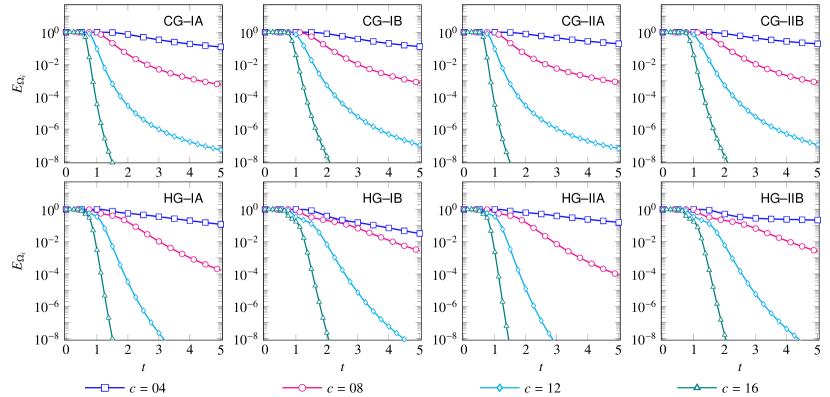
In the regime NtNmuch-greater-thansubscript𝑁𝑡𝑁N_{t}\gg N, say, Nt=𝒪(N2)subscript𝑁𝑡𝒪superscript𝑁2N_{t}=\mathop{\mathscr{O}}\left(N^{2}\right), the cost of computation scales as 𝒪(N4)𝒪superscript𝑁4\mathop{\mathscr{O}}\left(N^{4}\right) which corresponds to cost of computing the history functions while the memory requirement scales as 𝒪(N5)𝒪superscript𝑁5\mathop{\mathscr{O}}\left(N^{5}\right) .

3.3.2 NP–BDF1

Let us recall that, on the boundary segments Γa1subscriptΓsubscript𝑎1\Gamma_{a_{1}} and Γa2subscriptΓsubscript𝑎2\Gamma_{a_{2}}, the auxiliary fields are denoted by φk,a1(y2,τ1,τ2)subscript𝜑𝑘subscript𝑎1subscript𝑦2subscript𝜏1subscript𝜏2\varphi_{k,a_{1}}(y_{2},\tau_{1},\tau_{2}) and φk,a2(y1,τ1,τ2)subscript𝜑𝑘subscript𝑎2subscript𝑦1subscript𝜏1subscript𝜏2\varphi_{k,a_{2}}(y_{1},\tau_{1},\tau_{2}), respectively, while the auxiliary field at the corners is denoted by ψk,k,a1,a2(τ1,τ2)subscript𝜓𝑘superscript𝑘subscript𝑎1subscript𝑎2subscript𝜏1subscript𝜏2\psi_{k,k^{\prime},a_{1},a_{2}}(\tau_{1},\tau_{2}) where a1{l,r},a2{b,t}formulae-sequencesubscript𝑎1𝑙𝑟subscript𝑎2𝑏𝑡a_{1}\in\{l,r\},\;a_{2}\in\{b,t\} and k,k=1,2,,Mformulae-sequence𝑘superscript𝑘12𝑀k,k^{\prime}=1,2,\ldots,M. Let N𝑁N be the number of spatial nodes along y1subscript𝑦1y_{1} as well as y2subscript𝑦2y_{2}, i.e., N1=N2=Nsubscript𝑁1subscript𝑁2𝑁N_{1}=N_{2}=N. The storage of the auxiliary fields on the boundary segments require four 2D-arrays of size M×N𝑀𝑁M\times N and the storage of auxiliary field at corner points require four 2D-arrays of size M×M𝑀𝑀M\times M where M(<N)annotated𝑀absent𝑁M(<N) is the order of the diagonal Padé approximants used in the NP method. The evolution of these fields are effectively local in time which circumvents the need to store the history of these fields in time. The algorithmic steps for the solving the IBVP are enumerated below.

  1. Step 1:

    Advance the following IVPs corresponding to auxiliary fields by one step , say, j(j+1)𝑗𝑗1j\rightarrow(j+1) using the previously computed values of the auxiliary field on the segments (as described in Fig. 3):

    α12y12φk,a2j+1,j+φk,a2j+1,j=φk,a2j,j,α12y22φk,a1j,j+1+φk,a1j,j+1=φk,a1j,j,k=1,2,,M,formulae-sequencesubscriptsuperscript𝛼21superscriptsubscriptsubscript𝑦12subscriptsuperscript𝜑𝑗1𝑗𝑘subscript𝑎2subscriptsuperscript𝜑𝑗1𝑗𝑘subscript𝑎2subscriptsuperscript𝜑𝑗𝑗𝑘subscript𝑎2formulae-sequencesubscriptsuperscript𝛼21superscriptsubscriptsubscript𝑦22subscriptsuperscript𝜑𝑗𝑗1𝑘subscript𝑎1subscriptsuperscript𝜑𝑗𝑗1𝑘subscript𝑎1subscriptsuperscript𝜑𝑗𝑗𝑘subscript𝑎1𝑘12𝑀-\alpha^{-2}_{1}\partial_{y_{1}}^{2}\varphi^{j+1,j}_{k,a_{2}}+\varphi^{j+1,j}_{k,a_{2}}=\varphi^{j,j}_{k,a_{2}},\quad-\alpha^{-2}_{1}\partial_{y_{2}}^{2}\varphi^{j,j+1}_{k,a_{1}}+\varphi^{j,j+1}_{k,a_{1}}=\varphi^{j,j}_{k,a_{1}},\quad k=1,2,\ldots,M,

    together with the boundary conditions

    n2φk,a1j,j+1+α2ϖφk,a1j,j+1=α2k,a1,a2j+1,n1φk,a2j+1,j+α1ϖφk,a2j+1,j=α1k,a2,a1j+1,formulae-sequencesubscriptsubscript𝑛2superscriptsubscript𝜑𝑘subscript𝑎1𝑗𝑗1subscript𝛼2italic-ϖsuperscriptsubscript𝜑𝑘subscript𝑎1𝑗𝑗1subscript𝛼2subscriptsuperscript𝑗1𝑘subscript𝑎1subscript𝑎2subscriptsubscript𝑛1superscriptsubscript𝜑𝑘subscript𝑎2𝑗1𝑗subscript𝛼1italic-ϖsuperscriptsubscript𝜑𝑘subscript𝑎2𝑗1𝑗subscript𝛼1subscriptsuperscript𝑗1𝑘subscript𝑎2subscript𝑎1\partial_{n_{2}}\varphi_{k,a_{1}}^{j,j+1}+\alpha_{2}\varpi\varphi_{k,a_{1}}^{j,j+1}=-\alpha_{2}\mathcal{B}^{j+1}_{k,a_{1},a_{2}},\quad\partial_{n_{1}}\varphi_{k,a_{2}}^{j+1,j}+\alpha_{1}\varpi\varphi_{k,a_{2}}^{j+1,j}=-\alpha_{1}\mathcal{B}^{j+1}_{k,a_{2},a_{1}},

    where the history functions are given by

    k,a1,a2j+1=k=1MΓkψk,k,a1,a2j,j,k,a2,a1j+1=k=1MΓkψk,k,a2,a1j,j=k=1MΓkψk,k,a1,a2j,j.formulae-sequencesubscriptsuperscript𝑗1𝑘subscript𝑎1subscript𝑎2superscriptsubscriptsuperscript𝑘1𝑀subscriptΓsuperscript𝑘superscriptsubscript𝜓𝑘superscript𝑘subscript𝑎1subscript𝑎2𝑗𝑗subscriptsuperscript𝑗1𝑘subscript𝑎2subscript𝑎1superscriptsubscriptsuperscript𝑘1𝑀subscriptΓsuperscript𝑘superscriptsubscript𝜓𝑘superscript𝑘subscript𝑎2subscript𝑎1𝑗𝑗superscriptsubscriptsuperscript𝑘1𝑀subscriptΓsuperscript𝑘superscriptsubscript𝜓superscript𝑘𝑘subscript𝑎1subscript𝑎2𝑗𝑗\mathcal{B}^{j+1}_{k,a_{1},a_{2}}=\sum_{k^{\prime}=1}^{M}\Gamma_{k^{\prime}}\psi_{k,k^{\prime},a_{1},a_{2}}^{j,j},\quad\mathcal{B}^{j+1}_{k,a_{2},a_{1}}=\sum_{k^{\prime}=1}^{M}\Gamma_{k^{\prime}}\psi_{k,k^{\prime},a_{2},a_{1}}^{j,j}=\sum_{k^{\prime}=1}^{M}\Gamma_{k^{\prime}}\psi_{k^{\prime},k,a_{1},a_{2}}^{j,j}.

    These boundary condition are taken from Sec. 3.1 where precise definition of the quantities are provided. The cost of the steps outlined here works out to be 4MΘ1(N1)+4M24𝑀subscriptΘ1𝑁14superscript𝑀24M\Theta_{1}(N-1)+4M^{2} where the second part is the cost of computing the history functions. The memory requirement is 4MN+4M24𝑀𝑁4superscript𝑀24MN+4M^{2} size array.

  2. Step 2:

    Compute the history functions on the boundary segments of the domain ΩisubscriptΩ𝑖\Omega_{i} as

    a1j+1(y2)=k=1MΓkφk,a1j,j+1,a2j+1(y1)=k=1MΓkφk,a2j+1,j.formulae-sequencesubscriptsuperscript𝑗1subscript𝑎1subscript𝑦2superscriptsubscript𝑘1𝑀subscriptΓ𝑘superscriptsubscript𝜑𝑘subscript𝑎1𝑗𝑗1subscriptsuperscript𝑗1subscript𝑎2subscript𝑦1superscriptsubscript𝑘1𝑀subscriptΓ𝑘superscriptsubscript𝜑𝑘subscript𝑎2𝑗1𝑗\mathcal{B}^{j+1}_{a_{1}}(y_{2})=\sum_{k=1}^{M}\Gamma_{k}\varphi_{k,a_{1}}^{j,j+1},\quad\mathcal{B}^{j+1}_{a_{2}}(y_{1})=\sum_{k=1}^{M}\Gamma_{k}\varphi_{k,a_{2}}^{j+1,j}.

    The cost of this step is 𝒪(MN)𝒪𝑀𝑁\mathop{\mathscr{O}}\left(MN\right).

  3. Step 3:

    Solve the linear system for the interior problem to compute the solution at (j+1)𝑗1(j+1)-th time step

    (α12y12+α22y22)uj+1+uj+1=uj,ρ=1/Δt.formulae-sequencesubscriptsuperscript𝛼21subscriptsuperscript2subscript𝑦1subscriptsuperscript𝛼22subscriptsuperscript2subscript𝑦2superscript𝑢𝑗1superscript𝑢𝑗1superscript𝑢𝑗𝜌1Δ𝑡-\left(\alpha^{-2}_{1}\partial^{2}_{y_{1}}+\alpha^{-2}_{2}\partial^{2}_{y_{2}}\right)u^{j+1}+u^{j+1}=u^{j},\quad\rho=1/\Delta t.

    using the following Robin-type TBCs at discrete level

    n1uj+1+α1ϖuj+1=α1a1j+1(y2),n2uj+1+α2ϖuj+1=α2a2j+1(y1).formulae-sequencesubscriptsubscript𝑛1superscript𝑢𝑗1subscript𝛼1italic-ϖsuperscript𝑢𝑗1subscript𝛼1subscriptsuperscript𝑗1subscript𝑎1subscript𝑦2subscriptsubscript𝑛2superscript𝑢𝑗1subscript𝛼2italic-ϖsuperscript𝑢𝑗1subscript𝛼2subscriptsuperscript𝑗1subscript𝑎2subscript𝑦1\partial_{n_{1}}u^{j+1}+\alpha_{1}\varpi u^{j+1}=-\alpha_{1}\mathcal{B}^{j+1}_{a_{1}}(y_{2}),\quad\partial_{n_{2}}u^{j+1}+\alpha_{2}\varpi u^{j+1}=-\alpha_{2}\mathcal{B}^{j+1}_{a_{2}}(y_{1}).

    The cost of solving the linear system in this step works out to be Θ2(Ndim)=𝒪(N3)subscriptΘ2subscript𝑁dim𝒪superscript𝑁3\Theta_{2}(N_{\text{dim}})=\mathop{\mathscr{O}}\left(N^{3}\right) provided pivoting is not needed.

  4. Step 4:

    Update the 2D arrays storing the values of the auxiliary fields with the (j+1)𝑗1(j+1)-th time step values using the following update relations

    {φk,a1j+1,j+1=1(1+η¯k2)φk,a1j,j+1+1/ρ(1+η¯k2)uj+1,φk,a2j+1,j+1=1(1+η¯k2)φk,a2j+1,j+1/ρ(1+η¯k2)uj+1,and{ψk,k,a1a2j,j+1=1(1+η¯k2)ψk,k,a1,a2j,j+1/ρ(1+η¯k2)φk,a1j,j+1,ψk,k,a1a2j+1,j+1=1(1+η¯k2)ψk,k,a1,a2j,j+1+1/ρ(1+η¯k2)φk,a2j+1,j+1.\left\{\begin{aligned} &\varphi^{j+1,j+1}_{k,a_{1}}=\frac{1}{(1+\overline{\eta}^{2}_{k})}\varphi^{j,j+1}_{k,a_{1}}+\frac{1/\rho}{(1+\overline{\eta}^{2}_{k})}u^{j+1},\\ &\varphi^{j+1,j+1}_{k,a_{2}}=\frac{1}{(1+\overline{\eta}^{2}_{k})}\varphi^{j+1,j}_{k,a_{2}}+\frac{1/\rho}{(1+\overline{\eta}^{2}_{k})}u^{j+1},\end{aligned}\right.\quad\text{and}\quad\left\{\begin{aligned} &\psi^{j,j+1}_{k,k^{\prime},a_{1}a_{2}}=\frac{1}{(1+\overline{\eta}^{2}_{k^{\prime}})}\psi^{j,j}_{k,k^{\prime},a_{1},a_{2}}+\frac{1/\rho}{(1+\overline{\eta}^{2}_{k^{\prime}})}\varphi_{k,a_{1}}^{j,j+1},\\ &\psi^{j+1,j+1}_{k,k^{\prime},a_{1}a_{2}}=\frac{1}{(1+\overline{\eta}^{2}_{k})}\psi^{j,j+1}_{k,k^{\prime},a_{1},a_{2}}+\frac{1/\rho}{(1+\overline{\eta}^{2}_{k})}\varphi_{k^{\prime},a_{2}}^{j+1,j+1}.\end{aligned}\right.

From the discussion above, it is evident that the overall cost of computation is completely independent of the time-step and the DtN-maps get implemented at the cost of 𝒪(MN)𝒪𝑀𝑁\mathop{\mathscr{O}}\left(MN\right). The memory requirement for the auxiliary functions also remain independent of time-step with an estimate of 𝒪(MN)𝒪𝑀𝑁\mathop{\mathscr{O}}\left(MN\right). Therefore, the overall complexity is dominated by Θ2(Ndim)=𝒪(N3)subscriptΘ2subscript𝑁dim𝒪superscript𝑁3\Theta_{2}(N_{\text{dim}})=\mathop{\mathscr{O}}\left(N^{3}\right) which corresponds to the linear system for the interior problem.

Refer to caption
Figure 4: The figure shows the evolution of the relative energy content as defined in (177) of the chirped-Gaussian and the Hermite-Gaussian profiles considered in Table 1. Here the computational domain is Ωi=(10,10)2subscriptΩ𝑖superscript10102\Omega_{i}=(-10,10)^{2}.

4 Numerical Experiments

In this section, we will carry out the extensive numerical tests to showcase the accuracy of the numerical schemes developed in this work to solve the IBVP in (14). We start by analyzing the behaviour of the exact solutions for the IBVP under consideration followed by studying the error evolution behaviour and convergence analysis of the numerical schemes.

4.1 Exact solutions

The exact solutions admissible for our numerical experiments are such that the initial profile must be effectively supported within the computational domain. We primarily consider the wavepackets which are a modulation of a Gaussian envelop so that the requirement of effective initial support can be easily met. In this class of solutions, we consider the Chirped-Gaussian and the Hermite-Gaussian profiles.

Table 1: Chirped-Gaussian profile with A0=2subscript𝐴02A_{0}=2 and c0{4,8,12,16}subscript𝑐0481216c_{0}\in\{4,8,12,16\}.
G(𝒙,t)=A0j=1nG(𝒙,t;𝒂j,𝒃j,𝒄j),𝒄j=c0(cosθj,sinθj)formulae-sequence𝐺𝒙𝑡subscript𝐴0superscriptsubscript𝑗1𝑛𝐺𝒙𝑡subscript𝒂𝑗subscript𝒃𝑗subscript𝒄𝑗subscript𝒄𝑗subscript𝑐0subscript𝜃𝑗subscript𝜃𝑗G\left(\boldsymbol{x},t\right)=A_{0}\sum_{j=1}^{n}G(\boldsymbol{x},t;\boldsymbol{a}_{j},\boldsymbol{b}_{j},\boldsymbol{c}_{j}),\quad\boldsymbol{c}_{j}=c_{0}(\cos\theta_{j},\sin\theta_{j})
Type n𝑛n (𝒂j2)j=1nsuperscriptsubscriptsubscript𝒂𝑗superscript2𝑗1𝑛(\boldsymbol{a}_{j}\in\mathbb{R}^{2})_{j=1}^{n} (𝒃j2)j=1nsuperscriptsubscriptsubscript𝒃𝑗superscript2𝑗1𝑛(\boldsymbol{b}_{j}\in\mathbb{R}^{2})_{j=1}^{n} 𝜽n𝜽superscript𝑛\boldsymbol{\theta}\in\mathbb{R}^{n}
IA,
IB
222 𝒂1=(1/2.5,1/2.4)subscript𝒂112.512.4\boldsymbol{a}_{1}=(1/2.5,1/2.4),
𝒂2=(1/2.3,1/2.2)subscript𝒂212.312.2\boldsymbol{a}_{2}=(1/2.3,1/2.2)
𝒃j=(1/2)𝟏subscript𝒃𝑗121\boldsymbol{b}_{j}=(1/2)\boldsymbol{1} IA: 𝜽A=(0,π)subscript𝜽𝐴0𝜋\boldsymbol{\theta}_{A}=(0,\pi),
IB: 𝜽B=𝜽A+(π/4)𝟏subscript𝜽𝐵subscript𝜽𝐴𝜋41\boldsymbol{\theta}_{B}=\boldsymbol{\theta}_{A}+(\pi/4)\boldsymbol{1}
IIA,
IIB
444 𝒂1=(1/2.5,1/2.4)subscript𝒂112.512.4\boldsymbol{a}_{1}=(1/2.5,1/2.4),
𝒂2=(1/2.3,1/2.2)subscript𝒂212.312.2\boldsymbol{a}_{2}=(1/2.3,1/2.2),
𝒂3=(1/2.7,1/2.6)subscript𝒂312.712.6\boldsymbol{a}_{3}=(1/2.7,1/2.6),
𝒂4=(1/2.2,1/2.5)subscript𝒂412.212.5\boldsymbol{a}_{4}=(1/2.2,1/2.5)
𝒃j=(1/2)𝟏subscript𝒃𝑗121\boldsymbol{b}_{j}=(1/2)\boldsymbol{1} IIA: 𝜽A=(0,π/2,π,3π/2)subscript𝜽𝐴0𝜋2𝜋3𝜋2\boldsymbol{\theta}_{A}=(0,\pi/2,\pi,3\pi/2),
IIB: 𝜽B=𝜽A+(π/4)𝟏subscript𝜽𝐵subscript𝜽𝐴𝜋41\boldsymbol{\theta}_{B}=\boldsymbol{\theta}_{A}+(\pi/4)\boldsymbol{1}

4.1.1 Chirped-Gaussian profile

Using the function defined by

𝒢(x,t;a,b)=11+4i(a+ib)texp[(a+ib)1+4i(a+ib)tx2],a>0,b,formulae-sequence𝒢𝑥𝑡𝑎𝑏114𝑖𝑎𝑖𝑏𝑡𝑎𝑖𝑏14𝑖𝑎𝑖𝑏𝑡superscript𝑥2formulae-sequence𝑎0𝑏\mathcal{G}(x,t;a,b)=\frac{1}{\sqrt{1+4i(a+ib)t}}\exp\left[-\frac{(a+ib)}{1+4i(a+ib)t}x^{2}\right],\quad a>0,\;b\in\mathbb{R}, (174)

one can define the family of solutions referred to as chirped-Gaussian profile by

G(𝒙,t;𝒂,𝒃,𝒄)=𝒢(x1c1t,t;a1,b1)𝒢(x2c2t,t;a2,b2)exp(+i12𝒄𝒙i14𝒄𝒄t),𝐺𝒙𝑡𝒂𝒃𝒄𝒢subscript𝑥1subscript𝑐1𝑡𝑡subscript𝑎1subscript𝑏1𝒢subscript𝑥2subscript𝑐2𝑡𝑡subscript𝑎2subscript𝑏2𝑖12𝒄𝒙𝑖14𝒄𝒄𝑡G(\boldsymbol{x},t;\boldsymbol{a},\boldsymbol{b},\boldsymbol{c})=\mathcal{G}(x_{1}-c_{1}t,t;a_{1},b_{1})\mathcal{G}(x_{2}-c_{2}t,t;a_{2},b_{2})\exp\left(+i\frac{1}{2}\boldsymbol{c}\cdot\boldsymbol{x}-i\frac{1}{4}\boldsymbol{c}\cdot\boldsymbol{c}\,t\right), (175)

where 𝒂+2𝒂subscriptsuperscript2\boldsymbol{a}\in\mathbb{R}^{2}_{+} determines the effective support of the profile at t=0𝑡0t=0, 𝒃2𝒃superscript2\boldsymbol{b}\in\mathbb{R}^{2} is the chirp parameter and 𝒄2𝒄superscript2\boldsymbol{c}\in\mathbb{R}^{2} is the velocity of the profile. Using linear combination, one can further define a more general family of solutions with parameters A0,c0subscript𝐴0subscript𝑐0A_{0},c_{0}\in\mathbb{R}, 𝜽n𝜽superscript𝑛\boldsymbol{\theta}\in\mathbb{R}^{n}, (𝒂j+2)j=1nsuperscriptsubscriptsubscript𝒂𝑗subscriptsuperscript2𝑗1𝑛(\boldsymbol{a}_{j}\in\mathbb{R}^{2}_{+})_{j=1}^{n} and (𝒃j2)j=1nsuperscriptsubscriptsubscript𝒃𝑗superscript2𝑗1𝑛(\boldsymbol{b}_{j}\in\mathbb{R}^{2})_{j=1}^{n} given by

G(𝒙,t;c0,A0;(𝒂j)j=1n,(𝒃j)j=1n,𝜽)=A0j=1nG(𝒙,t;𝒂j,𝒃j,𝒄j),𝒄j=c0(cosθj,sinθj).formulae-sequence𝐺𝒙𝑡subscript𝑐0subscript𝐴0superscriptsubscriptsubscript𝒂𝑗𝑗1𝑛superscriptsubscriptsubscript𝒃𝑗𝑗1𝑛𝜽subscript𝐴0superscriptsubscript𝑗1𝑛𝐺𝒙𝑡subscript𝒂𝑗subscript𝒃𝑗subscript𝒄𝑗subscript𝒄𝑗subscript𝑐0subscript𝜃𝑗subscript𝜃𝑗G\left(\boldsymbol{x},t;\;c_{0},A_{0};\;(\boldsymbol{a}_{j})_{j=1}^{n},(\boldsymbol{b}_{j})_{j=1}^{n},\boldsymbol{\theta}\right)=A_{0}\sum_{j=1}^{n}G(\boldsymbol{x},t;\boldsymbol{a}_{j},\boldsymbol{b}_{j},\boldsymbol{c}_{j}),\quad\boldsymbol{c}_{j}=c_{0}(\cos\theta_{j},\sin\theta_{j}). (176)

Let the constant vector (1,1,)n11superscript𝑛(1,1,\ldots)\in\mathbb{R}^{n} be denoted by 𝟏1\boldsymbol{1}, then the specific values of the parameters of the solutions used in the numerical experiments can be summarized as in Table 1. The energy content of the profile within the computational domain ΩisubscriptΩ𝑖\Omega_{i} over time is

EΩi(t)=Ωi|G(𝒙,t)|2d2𝒙/Ωi|G(𝒙,0)|2d2𝒙,t0.formulae-sequencesubscript𝐸subscriptΩ𝑖𝑡subscriptsubscriptΩ𝑖/superscript𝐺𝒙𝑡2superscript𝑑2𝒙subscriptsubscriptΩ𝑖superscript𝐺𝒙02superscript𝑑2𝒙𝑡0E_{\Omega_{i}}(t)=\left.{\int_{\Omega_{i}}|G(\boldsymbol{x},t)|^{2}d^{2}\boldsymbol{x}}\right/{\int_{\Omega_{i}}|G(\boldsymbol{x},0)|^{2}d^{2}\boldsymbol{x}},\quad t\geq 0. (177)

The profiles are chosen with non-zero speed c0subscript𝑐0c_{0} so that the field hits the boundary of ΩisubscriptΩ𝑖\Omega_{i}, In case of a square computational domain, the type ‘A’ class of solutions are directed to the segments of the boundary normally while type ‘B’ class of solutions are directed to the corners. The behaviour of the EΩi(t)subscript𝐸subscriptΩ𝑖𝑡E_{\Omega_{i}}(t) for t[0,5]𝑡05t\in[0,5] is shown in Fig. 4.

Table 2: Hermite-Gaussian profile with A0=2subscript𝐴02A_{0}=2 and c0{4,8,12,16}subscript𝑐0481216c_{0}\in\{4,8,12,16\}.
G(𝒙,t)=A0j=1nG(𝒙,t;𝒎j,𝒂j,𝒄j),𝒄j=c0(cosθj,sinθj)formulae-sequence𝐺𝒙𝑡subscript𝐴0superscriptsubscript𝑗1𝑛𝐺𝒙𝑡subscript𝒎𝑗subscript𝒂𝑗subscript𝒄𝑗subscript𝒄𝑗subscript𝑐0subscript𝜃𝑗subscript𝜃𝑗G\left(\boldsymbol{x},t\right)=A_{0}\sum_{j=1}^{n}G(\boldsymbol{x},t;\boldsymbol{m}_{j},\boldsymbol{a}_{j},\boldsymbol{c}_{j}),\;\boldsymbol{c}_{j}=c_{0}(\cos\theta_{j},\sin\theta_{j})
Type n𝑛n (𝒂j2)j=1nsuperscriptsubscriptsubscript𝒂𝑗superscript2𝑗1𝑛(\boldsymbol{a}_{j}\in\mathbb{R}^{2})_{j=1}^{n} (𝒎j02)j=1nsuperscriptsubscriptsubscript𝒎𝑗superscriptsubscript02𝑗1𝑛(\boldsymbol{m}_{j}\in\mathbb{N}_{0}^{2})_{j=1}^{n} 𝜽n𝜽superscript𝑛\boldsymbol{\theta}\in\mathbb{R}^{n}
IA,
IB
222 𝒂1=(1/2.5,1/2.4)subscript𝒂112.512.4\boldsymbol{a}_{1}=(1/2.5,1/2.4),
𝒂2=(1/2.3,1/2.2)subscript𝒂212.312.2\boldsymbol{a}_{2}=(1/2.3,1/2.2)
𝒎1=(1,2)subscript𝒎112\boldsymbol{m}_{1}=(1,2),
𝒎2=(2,1)subscript𝒎221\boldsymbol{m}_{2}=(2,1)
𝜽A=(0,π)subscript𝜽𝐴0𝜋\boldsymbol{\theta}_{A}=(0,\pi),
𝜽B=𝜽A+(π/4)𝟏subscript𝜽𝐵subscript𝜽𝐴𝜋41\boldsymbol{\theta}_{B}=\boldsymbol{\theta}_{A}+(\pi/4)\boldsymbol{1}
IIA,
IIB
444 𝒂1=(1/2.5,1/2.4)subscript𝒂112.512.4\boldsymbol{a}_{1}=(1/2.5,1/2.4),
𝒂2=(1/2.3,1/2.2)subscript𝒂212.312.2\boldsymbol{a}_{2}=(1/2.3,1/2.2),
𝒂3=(1/2.7,1/2.6)subscript𝒂312.712.6\boldsymbol{a}_{3}=(1/2.7,1/2.6),
𝒂4=(1/2.2,1/2.5)subscript𝒂412.212.5\boldsymbol{a}_{4}=(1/2.2,1/2.5)
𝒎1=(1,2)subscript𝒎112\boldsymbol{m}_{1}=(1,2),
𝒎2=(2,1)subscript𝒎221\boldsymbol{m}_{2}=(2,1),
𝒎3=(2,1)subscript𝒎321\boldsymbol{m}_{3}=(2,1),
𝒎4=(1,2)subscript𝒎412\boldsymbol{m}_{4}=(1,2)
𝜽A=(0,π/2,π,3π/2)subscript𝜽𝐴0𝜋2𝜋3𝜋2\boldsymbol{\theta}_{A}=(0,\pi/2,\pi,3\pi/2),
𝜽B=𝜽A+(π/4)𝟏subscript𝜽𝐵subscript𝜽𝐴𝜋41\boldsymbol{\theta}_{B}=\boldsymbol{\theta}_{A}+(\pi/4)\boldsymbol{1}
Refer to caption
Figure 5: The figure shows the behaviour of error involved in the discretization of the boundary map alone for the chirped-Gaussian profile with different values of the speed ‘c’ (see Table 1). The numerical parameters and the labels are described in Sec. 4.2 where the error is quantified by (184).
Refer to caption
Figure 6: The figure shows the behaviour of error involved in the discretization of the boundary map alone for the Hermite-Gaussian profile with different values of the speed ‘c’ (see Table 2). The numerical parameters and the labels are described in Sec. 4.2 where the error is quantified by (184).
Refer to caption
Figure 7: The figure shows a comparison of evolution of error in the numerical solution of the IBVP (14) with the various TBCs for the chirped-Gaussian profile with different values of the speed ‘c’ (see Table 1). The numerical parameters and the labels are described in Sec. 4.3 where the error is quantified by (185).

4.1.2 Hermite-Gaussian profile

Consider the class of normalized Hermite-Gaussian functions defined by

𝒢m(x,t;a)=γm1Hm(2axw(t))μ(t)aexp[μ(t)x2imθ(t)],m0={0,1,},formulae-sequencesubscript𝒢𝑚𝑥𝑡𝑎superscriptsubscript𝛾𝑚1subscript𝐻𝑚2𝑎𝑥𝑤𝑡𝜇𝑡𝑎𝜇𝑡superscript𝑥2𝑖𝑚𝜃𝑡𝑚subscript001\mathcal{G}_{m}(x,t;a)=\gamma_{m}^{-1}H_{m}\left(\frac{\sqrt{2a}\,x}{w(t)}\right)\sqrt{\frac{\mu(t)}{a}}\exp\left[-\mu(t)x^{2}-i\,m\theta(t)\right],\quad m\in\mathbb{N}_{0}=\{0,1,\ldots\}, (178)

where a>0𝑎0a>0,

w(t)=1+(4at)2,1μ(t)=1a+i4t=1aw(t)exp[iθ(t)],formulae-sequence𝑤𝑡1superscript4𝑎𝑡21𝜇𝑡1𝑎𝑖4𝑡1𝑎𝑤𝑡𝑖𝜃𝑡w(t)=\sqrt{1+(4at)^{2}},\quad\frac{1}{\mu(t)}=\frac{1}{a}+i{4t}=\frac{1}{a}w(t)\exp[i\theta(t)], (179)

and the normalization factor is given by γm2=2m(m!)π(2a)1/2subscriptsuperscript𝛾2𝑚superscript2𝑚𝑚𝜋superscript2𝑎12\gamma^{2}_{m}=2^{m}(m!)\sqrt{\pi}(2a)^{-1/2}.

The Hermite polynomials are evaluated using the following relations

Hn+1(x)=2xHn(x)2nHn1(x),Hn+1(x)=2(n+1)Hn(x),formulae-sequencesubscript𝐻𝑛1𝑥2𝑥subscript𝐻𝑛𝑥2𝑛subscript𝐻𝑛1𝑥superscriptsubscript𝐻𝑛1𝑥2𝑛1subscript𝐻𝑛𝑥H_{n+1}(x)=2xH_{n}(x)-2nH_{n-1}(x),\quad H_{n+1}^{\prime}(x)=2(n+1)H_{n}(x), (180)

with H0(x)=1subscript𝐻0𝑥1H_{0}(x)=1 and H1(x)=2xsubscript𝐻1𝑥2𝑥H_{1}(x)=2x, These relations can be used to compute the first spatial derivative of the Hermite-Gaussian functions:

x𝒢m(x,t;a)=(m+1)a𝒢m+1(x,t;a)+ma𝒢m1(x,t;a),m>0,formulae-sequencesubscript𝑥subscript𝒢𝑚𝑥𝑡𝑎𝑚1𝑎subscript𝒢𝑚1𝑥𝑡𝑎𝑚𝑎subscript𝒢𝑚1𝑥𝑡𝑎𝑚0\partial_{x}\mathcal{G}_{m}(x,t;a)=-\sqrt{(m+1)a}\mathcal{G}_{m+1}(x,t;a)+\sqrt{ma}\mathcal{G}_{m-1}(x,t;a),\quad m>0, (181)

with x𝒢0(x,t;a)=a𝒢1(x,t;a)subscript𝑥subscript𝒢0𝑥𝑡𝑎𝑎subscript𝒢1𝑥𝑡𝑎\partial_{x}\mathcal{G}_{0}(x,t;a)=-\sqrt{a}\mathcal{G}_{1}(x,t;a). This is required for testing our Dirichlet-to-Neumann maps. Using these functions, we can define a family of solutions referred to as Hermite-Gaussian profile by

G(𝒙,t;𝒎,𝒂,𝒄)=𝒢m1(x1c1t,t;a1)𝒢m2(x2c2t,t;a2)exp(+i12𝒄𝒙i14𝒄𝒄t),𝐺𝒙𝑡𝒎𝒂𝒄subscript𝒢subscript𝑚1subscript𝑥1subscript𝑐1𝑡𝑡subscript𝑎1subscript𝒢subscript𝑚2subscript𝑥2subscript𝑐2𝑡𝑡subscript𝑎2𝑖12𝒄𝒙𝑖14𝒄𝒄𝑡G(\boldsymbol{x},t;\boldsymbol{m},\boldsymbol{a},\boldsymbol{c})=\mathcal{G}_{m_{1}}(x_{1}-c_{1}t,t;a_{1})\mathcal{G}_{m_{2}}(x_{2}-c_{2}t,t;a_{2})\exp\left(+i\frac{1}{2}\boldsymbol{c}\cdot\boldsymbol{x}-i\frac{1}{4}\boldsymbol{c}\cdot\boldsymbol{c}\,t\right), (182)

where 𝒎02𝒎superscriptsubscript02\boldsymbol{m}\in\mathbb{N}_{0}^{2} is the order parameter, 𝒂+2𝒂subscriptsuperscript2\boldsymbol{a}\in\mathbb{R}^{2}_{+} determines the effective support of the profile at t=0𝑡0t=0 and 𝒄2𝒄superscript2\boldsymbol{c}\in\mathbb{R}^{2} is the velocity of the profile. Once again, using linear combination, one can further define a more general family of solutions with parameters A0,c0subscript𝐴0subscript𝑐0A_{0},c_{0}\in\mathbb{R}, 𝜽n𝜽superscript𝑛\boldsymbol{\theta}\in\mathbb{R}^{n}, (𝒎j02)j=1nsuperscriptsubscriptsubscript𝒎𝑗subscriptsuperscript20𝑗1𝑛(\boldsymbol{m}_{j}\in\mathbb{N}^{2}_{0})_{j=1}^{n} and (𝒂j+2)j=1nsuperscriptsubscriptsubscript𝒂𝑗subscriptsuperscript2𝑗1𝑛(\boldsymbol{a}_{j}\in\mathbb{R}^{2}_{+})_{j=1}^{n} given by

G(𝒙,t;c0,A0;(𝒎j)j=1n,(𝒂j)j=1n,𝜽)=A0j=1nG(𝒙,t;𝒎j,𝒂j,𝒄j),𝒄j=c0(cosθj,sinθj).formulae-sequence𝐺𝒙𝑡subscript𝑐0subscript𝐴0superscriptsubscriptsubscript𝒎𝑗𝑗1𝑛superscriptsubscriptsubscript𝒂𝑗𝑗1𝑛𝜽subscript𝐴0superscriptsubscript𝑗1𝑛𝐺𝒙𝑡subscript𝒎𝑗subscript𝒂𝑗subscript𝒄𝑗subscript𝒄𝑗subscript𝑐0subscript𝜃𝑗subscript𝜃𝑗G\left(\boldsymbol{x},t;\;c_{0},A_{0};\;(\boldsymbol{m}_{j})_{j=1}^{n},(\boldsymbol{a}_{j})_{j=1}^{n},\boldsymbol{\theta}\right)=A_{0}\sum_{j=1}^{n}G(\boldsymbol{x},t;\boldsymbol{m}_{j},\boldsymbol{a}_{j},\boldsymbol{c}_{j}),\quad\boldsymbol{c}_{j}=c_{0}(\cos\theta_{j},\sin\theta_{j}). (183)

As in the last case, we set 𝟏=(1,1,)n111superscript𝑛\boldsymbol{1}=(1,1,\ldots)\in\mathbb{R}^{n}, then the specific values of the parameters of the solutions used in the numerical experiments can be summarized as in Table 2. The energy content of the profile within the computational domain ΩisubscriptΩ𝑖\Omega_{i} over time is EΩi(t)subscript𝐸subscriptΩ𝑖𝑡E_{\Omega_{i}}(t) as defined by (177) with the appropriate profile in the integrand. The profiles are chosen with non-zero speed c0subscript𝑐0c_{0} so that the field hits the boundary of ΩisubscriptΩ𝑖\Omega_{i}. In case of a square computational domain, the type ‘A’ class of solutions are directed to the segments of the boundary normally while type ‘B’ class of solutions are directed to the corners. The behaviour of the EΩi(t)subscript𝐸subscriptΩ𝑖𝑡E_{\Omega_{i}}(t) for t[0,5]𝑡05t\in[0,5] is shown in Fig. 4.

Refer to caption
Figure 8: The figure shows a comparison of evolution of error in the numerical solution of the IBVP (14) with the various TBCs for the Hermite-Gaussian profile with different values of the speed ‘c’ (see Table 2). The numerical parameters and the labels are described in Sec. 4.3 where the error is quantified by (185).

4.2 Tests for DtN maps

Prior to the full implementation of the numerical scheme, one can test the accuracy of the DtN boundary maps where we quantify the error on ΩisubscriptΩ𝑖\partial\Omega_{i} by

e(tj)=(Ωi|nu(𝒙,tj)[nu(𝒙,tj)]num.|2𝑑σ(𝒙))1/2,tj[0,Tmax],formulae-sequence𝑒subscript𝑡𝑗superscriptsubscriptsubscriptΩ𝑖superscriptsubscript𝑛𝑢𝒙subscript𝑡𝑗subscriptdelimited-[]subscript𝑛𝑢𝒙subscript𝑡𝑗num.2differential-d𝜎𝒙12subscript𝑡𝑗0subscript𝑇𝑚𝑎𝑥e(t_{j})=\left(\int_{\partial\Omega_{i}}\left|\partial_{n}u(\boldsymbol{x},t_{j})-[\partial_{n}u(\boldsymbol{x},t_{j})]_{\text{num.}}\right|^{2}d\sigma(\boldsymbol{x})\right)^{1/2},\quad t_{j}\in[0,T_{max}], (184)

where dσ(𝒙)𝑑𝜎𝒙d\sigma(\boldsymbol{x}) denotes the measure along the boundary of the computational domain ΩisubscriptΩ𝑖\Omega_{i}. Along the spatial dimension, the integral above will be approximated by Gauss quadrature over LGL-points 444The quadrature nodes and the corresponding weights are computed using quad precision in order to avoid any numerical artifacts due to round-off errors.. The quantity [nu(𝒙,tj)]num.subscriptdelimited-[]subscript𝑛𝑢𝒙subscript𝑡𝑗num.[\partial_{n}u(\boldsymbol{x},t_{j})]_{\text{num.}} refers to the numerical approximation of the Neumann datum from the Dirichlet datum. All the intermediate quantities involved in this process is computed according to a numerical scheme developed as part of the numerical realization of the DtN map.

In this work, we have developed two discrete versions of the DtN maps, namely, CQ and NP. Each of these methods have a variant determined by the choice of one-step method used in the temporal discretization so that the complete list of methods to be tested can be labelled as CQ–BDF1, NP–BDF1 (corresponding to the one-step method BDF1), and, CQ–TR, NP–TR (corresponding to the one-step method TR). For the Padé approximant based method ‘NP’, we distinguish the diagonal approximant of order 202020 from that of 505050 via the labels ‘NP20’ and ‘NP50’. The numerical parameters used in this section are summarized in Table 3. The exact solutions used are described in Sec. 4.1. Let us note that the accuracy of the DtN maps do not reflect the accuracy of the numerical solution computed with the TBCs on account of the fact that the interior problem together with the discretized DtN maps may turn out to be unstable.

Table 3: Numerical parameters for testing DtN maps
Computational domain (ΩisubscriptΩ𝑖\Omega_{i}) (10,10)×(10,10)10101010(-10,10)\times(-10,10)
Maximum time (Tmaxsubscript𝑇𝑚𝑎𝑥T_{max}) 222
No. of time-steps (Ntsubscript𝑁𝑡N_{t}) 1000+1100011000+1
Time-step (ΔtΔ𝑡\Delta t) 2×103=Tmax/(Nt1)2superscript103subscript𝑇𝑚𝑎𝑥subscript𝑁𝑡12\times 10^{-3}=T_{max}/(N_{t}-1)
Number of LGL-points (N+1𝑁1N+1) 200200200

The numerical results for error on ΩisubscriptΩ𝑖\partial\Omega_{i} corresponding to the chirped-Gaussian and the Hermite-Gaussian profiles are shown in Fig. 5 and Fig. 6, respectively. It can be seen that the diagonal Padé approximant based methods, namely, NP20 and NP50, perform equally well as compared to that of the convolution quadrature based method. Moreover, the TR methods perform better than the BDF1 methods which is clear from the error peaks in figures 5 and 6. The accuracy deteriorates with increase in the value of c𝑐c. For faster moving profiles corresponding to IA and IIA type solutions, NP-20 becomes slightly less accurate compared to CQ and NP-50. There is no significant difference in the results for error on ΩisubscriptΩ𝑖\partial\Omega_{i} corresponding to the chirped-Gaussian profile and the Hermite-Gaussian profile.
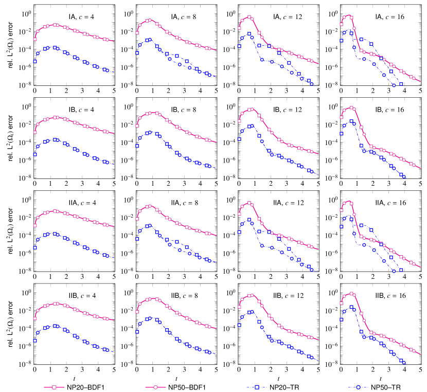
Refer to caption
Figure 9: The figure shows a comparison of evolution of error in the numerical solution of the IBVP (14) with the TBCs developed using novel Padé approach for the chirped-Gaussian profile with different values of the speed ‘c’ (see Table 1). The numerical parameters and the labels are described in Sec. 4.3 where the error is quantified by (185).
Refer to caption
Figure 10: The figure shows a comparison of evolution of error in the numerical solution of the IBVP (14) with the TBCs developed using novel Padé approach for the Hermite-Gaussian profile with different values of the speed ‘c’ (see Table 2). The numerical parameters and the labels are described in Sec. 4.3 where the error is quantified by (185).

4.3 Tests for evolution error

In this section, we consider the IBVP in (14) where the initial condition corresponds to the exact solutions described in Sec. 4.1. The numerical solution is labelled according to that of the boundary maps described in Sec. 4.2. The error in the evolution of the profile computed numerically is quantified by the relative 𝖫2(Ωi)superscript𝖫2subscriptΩ𝑖\mathsf{L}^{2}(\Omega_{i})-norm:

e(tj)=(Ωi|u(𝒙,tj)[u(𝒙,tj)]num.|2d2𝒙)1/2/(Ωi|u0(𝒙)|2d2𝒙)1/2,𝑒subscript𝑡𝑗/superscriptsubscriptsubscriptΩ𝑖superscript𝑢𝒙subscript𝑡𝑗subscriptdelimited-[]𝑢𝒙subscript𝑡𝑗num.2superscript𝑑2𝒙12superscriptsubscriptsubscriptΩ𝑖superscriptsubscript𝑢0𝒙2superscript𝑑2𝒙12e(t_{j})=\left.\left(\int_{\Omega_{i}}\left|u(\boldsymbol{x},t_{j})-[u(\boldsymbol{x},t_{j})]_{\text{num.}}\right|^{2}d^{2}\boldsymbol{x}\right)^{1/2}\,\right/\left(\int_{\Omega_{i}}\left|u_{0}(\boldsymbol{x})\right|^{2}d^{2}\boldsymbol{x}\right)^{1/2}, (185)

for tj[0,Tmax]subscript𝑡𝑗0subscript𝑇𝑚𝑎𝑥t_{j}\in[0,T_{max}]. The integral above will be approximated by Gauss quadrature over LGL-points.

For Padé based discretization (NP) of the DtN maps, it is possible to carry out evolution over larger number of time-steps. The Table 4 lists the numerical parameters for the NP20 and NP50 methods. The CQ based methods cannot be tested with the same parameters on account of the increasing memory requirements at each time-step. Therefore, we introduce a separate test-case for the sake of comparison with CQ methods by restricting Nt=1000+1subscript𝑁𝑡10001N_{t}=1000+1 and Tmax=2subscript𝑇𝑚𝑎𝑥2T_{max}=2 while other parameters are same as that of Table 4.

The numerical results for the evolution error on ΩisubscriptΩ𝑖\Omega_{i} corresponding to the chirped-Gaussian and the Hermite-Gaussian profiles are shown in Fig. 7 and Fig. 8, respectively. It can be seen that the diagonal Padé approximants based method, namely, NP20 and NP50, perform equally well as compared to that of the convolution quadrature based method. Moreover, the TR methods perform better than the BDF1 methods which is clear from the error peaks in figures 7 and 8. The accuracy deteriorates with increase in the value of c𝑐c. For faster moving profiles corresponding to IA and IIA type solutions, NP-20 becomes slightly less accurate compared to CQ and NP-50. There is no significant difference in the results for evolution error on ΩisubscriptΩ𝑖\Omega_{i} corresponding to the chirped-Gaussian profile and the Hermite-Gaussian profile.
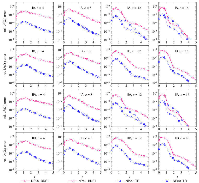
The numerical results for the evolution error on ΩisubscriptΩ𝑖\Omega_{i} particularly for NP methods corresponding to the chirped-Gaussian and Hermite-Gaussian profiles are shown in Fig. 9 and Fig. 10, respectively. Note that the results for NP are superior than that of CQ on account of the reduced size (ΔtΔ𝑡\Delta t) of the time-step which was possible because increasing the number of time-steps did not significantly increase the computation time as well as memory requirements unlike that of CQ555Attempts to lower the step-size for the same maximum duration of time in case of CQ failed due to out-of-memory errors. We note that these problems may severely limit the practical utility of the CQ method..

Table 4: Numerical parameters for studying the evolution error for the NP methods
Computational domain (ΩisubscriptΩ𝑖\Omega_{i}) (10,10)×(10,10)10101010(-10,10)\times(-10,10)
Maximum time (Tmaxsubscript𝑇𝑚𝑎𝑥T_{max}) 555
No. of time-steps (Ntsubscript𝑁𝑡N_{t}) 5000+1500015000+1
Time-step (ΔtΔ𝑡\Delta t) 103=Tmax/(Nt1)superscript103subscript𝑇𝑚𝑎𝑥subscript𝑁𝑡110^{-3}=T_{max}/(N_{t}-1)
Number of LGL-points ((N+1)×(N+1)𝑁1𝑁1(N+1)\times(N+1)) 200×200200200200\times 200

In order to visualize the reflections at the boundary, we resort to contour plots depicting the quantity fmag.log10|u(𝒙,t)|subscript𝑓mag.subscript10𝑢𝒙𝑡f_{\text{mag.}}\log_{10}|u(\boldsymbol{x},t)| where the scalar quantity fmag.subscript𝑓mag.f_{\text{mag.}} is adjusted to resolve the contour lines properly. The specific snapshots correspond to the equispaced energy levels in the logarithmic scale that is remaining in the computational domain. We restrict ourselves to presenting the contour plots only for the case of type IIB class of solutions which are directed towards the corners of the domain on account of being most complex among four different class of solutions. The contour plots depicting corresponding to the chirped-Gaussian (fmag.=4subscript𝑓mag.4f_{\text{mag.}}=4) and the Hermite-Gaussian (fmag.=8subscript𝑓mag.8f_{\text{mag.}}=8) profiles are shown in Fig. 13 and Fig. 14, respectively. The top row corresponds to the exact solution for reference. From these plots, we conclude that the results are similar for each of the types of solutions. There are minimal visible reflections in the contour plots proving the accuracy of the developed numerical schemes to implement the TBCs. Moreover, the TR based methods better resolve the contour levels in comparison to the BDF1 based methods.

Table 5: Numerical parameters for studying the convergence error for the NP methods
Computational domain (ΩisubscriptΩ𝑖\Omega_{i}) (10,10)×(10,10)10101010(-10,10)\times(-10,10)
Maximum time (Tmaxsubscript𝑇𝑚𝑎𝑥T_{max}) 555
Set of no. of time-steps (tsubscript𝑡\mathbb{N}_{t}) {28,29,,218}superscript28superscript29superscript218\{2^{8},2^{9},\ldots,2^{18}\}
Time-step {Δt=Tmax/(Nt1),Ntt}formulae-sequenceΔ𝑡subscript𝑇𝑚𝑎𝑥subscript𝑁𝑡1subscript𝑁𝑡subscript𝑡\{\Delta t=T_{max}/(N_{t}-1),\;N_{t}\in\mathbb{N}_{t}\}
Number of LGL-points ((N+1)×(N+1)𝑁1𝑁1(N+1)\times(N+1)) 200×200200200200\times 200

4.4 Tests for convergence

In this section, we analyze the convergence behaviour of the numerical schemes for the IBVP in (14) where the initial condition corresponds to the exact solutions described in Sec. 4.1. The numerical solution is labelled according to that of the boundary maps described in Sec. 4.2.

The error used to study the convergence behaviour is quantified by the maximum relative 𝖫2(Ωi)superscript𝖫2subscriptΩ𝑖\mathsf{L}^{2}(\Omega_{i})-norm:

e=max{e(tj)|j=0,1,,Nt1},𝑒conditional𝑒subscript𝑡𝑗𝑗01subscript𝑁𝑡1e=\max\left\{e(t_{j})|\;j=0,1,\ldots,N_{t}-1\right\}, (186)

for tj[0,Tmax]subscript𝑡𝑗0subscript𝑇𝑚𝑎𝑥t_{j}\in[0,T_{max}]. For Padé based discretization (NP) of the DtN maps, it is possible to analyze the convergence behaviour over large number of time-steps. The Table 5 lists the numerical parameters for the NP20 and NP50 methods. The CQ based methods cannot be tested with the same parameters on account of the increasing memory requirements at each time-step.
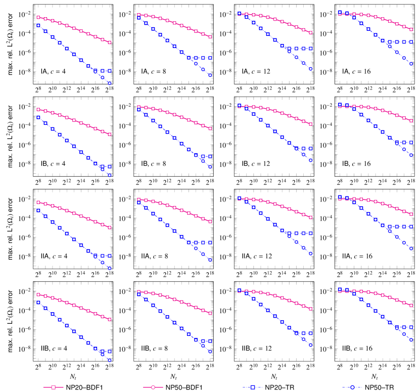
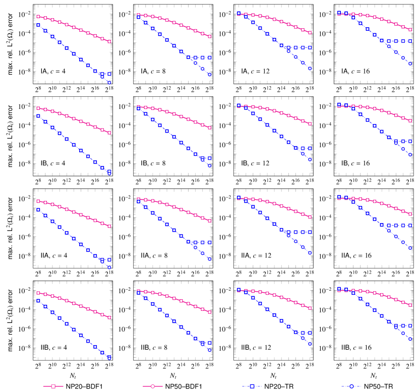
Refer to caption
Figure 11: The figure depicts the convergence behaviour of the numerical solution of the IBVP (14) with the TBCs developed using novel Padé approach for the chirped-Gaussian profile with different values of the speed ‘c’ (see Table 1). The numerical parameters and the labels are described in Sec. 4.4 where the error is quantified by (186).
Refer to caption
Figure 12: The figure depicts the convergence behaviour of the numerical solution of the IBVP (14) with the TBCs developed using novel Padé approach for the Hermite-Gaussian profile with different values of the speed ‘c’ (see Table 2). The numerical parameters and the labels are described in Sec. 4.4 where the error is quantified by (186).

The numerical results for the convergence behaviour on ΩisubscriptΩ𝑖\Omega_{i} corresponding to the chirped-Gaussian and the Hermite-Gaussian profiles are shown in Fig. 11 and Fig. 12, respectively. It can be seen that the diagonal Padé approximant based method, namely, NP20 and NP50, shows stable behaviour for the parameters specified in Table 5. In the log-log scale, we can clearly identify the error curve to be a straight line before it plateaus. The orders can be recovered from the slope which we found consistent with the order of the underlying one-step method. The TR methods perform better than the BDF1 methods which is obvious from the slope of the error curves in figures 11 and 12. We note that the error background increases with increase in the value of c𝑐c. This is on account of the increased oscillatory behaviour of the solution in t𝑡t as c𝑐c increases and a method with higher order than 222 would be required to achieve the same accuracy as that of the slow moving profiles keeping the step-size same. Note that NP20 methods starts plateauing after a certain number of time-steps unlike NP50. This can be attributed to the approximate nature of the TBCs with a lower order of diagonal approximants chosen. Finally, let us observe that there is no significant difference in the results for convergence on ΩisubscriptΩ𝑖\Omega_{i} corresponding to the chirped-Gaussian profile and the Hermite-Gaussian profile.

5 Conclusion

In this paper, we presented a new effectively local approximation for the numerical realization of the TBCs on a rectangular computational domain for the free Schrödinger equation in 2superscript2\mathbb{R}^{2}. Our starting point was a numerically tractable formulation of the transparent boundary operator, tiΓsubscript𝑡𝑖subscriptΓ\sqrt{\partial_{t}-i\triangle_{\Gamma}}, where ΓsubscriptΓ\triangle_{\Gamma} is the Laplace-Beltrami operator [4, 5], which is nonlocal in time as well as space. This formulation of the TBCs introduces an auxiliary function which happens to satisfy the one-dimensional Schrödinger equation along the boundary segments of the computational domain. It addressed the nonlocality in space, however, the nonlocality in time remained a serious bottleneck on account of the growing computational complexity with number of time-steps which becomes prohibitive after a point. To overcome this challenge, we developed a novel Padé approximant based rational approximation for the 1/2121/2-order time-fractional derivative. This approach circumvents the need to store the entire history of the field on the boundary segments and allows us to achieve a computational complexity that remains independent of the number of time-steps. Let us emphasize that our approach is significantly different from that of Menza [7] which fails at the corners of the rectangular domain. Further, we also present a convolution quadrature based scheme which happens to be computationally expensive but it is well-known as a golden standard for 1D problems. As far as time marching is concerned, we note that one-step methods are best suited for our purpose and any higher-order method can be readily used to implement our algorithm. These aspects will be further explored in a future publication.

For the spatial discretization, we use a Legendre-Galerkin spectral method with a new boundary adapted basis which leads to a banded linear system for the 1D problems on the boundary segments as well as for the interior problem. The time-discrete version of the boundary condition are formulated as a Robin-type condition in a manner reminiscent of the 1D problem [3]. A compatible boundary-lifting procedure to homogenize the Robin-type boundary conditions is also presented. In order to demonstrate the effectiveness of the methods developed, we carried out numerical tests to study the behaviour of evolution of error as well as to verify the order of convergence empirically. If the number of spatial grid points in every dimension is 𝒪(N)𝒪𝑁\mathop{\mathscr{O}}\left(N\right), then the computational complexity of our novel Padé method for the DtN map scales as 𝒪(MN)𝒪𝑀𝑁\mathop{\mathscr{O}}\left(MN\right) where M𝑀M is the order of the diagonal Padé approximant. Let us emphasize that this complexity is independent of the number of time-steps. The overall complexity thus becomes dominated by the cost of the linear solver for interior problem which is given by Θ2(Ndim)=𝒪(N3)subscriptΘ2subscript𝑁dim𝒪superscript𝑁3\Theta_{2}(N_{\text{dim}})=\mathop{\mathscr{O}}\left(N^{3}\right). A theoretical proof of the stability and convergence of the numerical scheme is beyond the scope of the paper. These issues are deferred to a future publication.
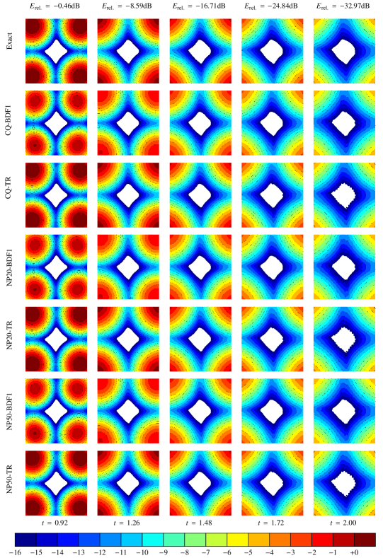
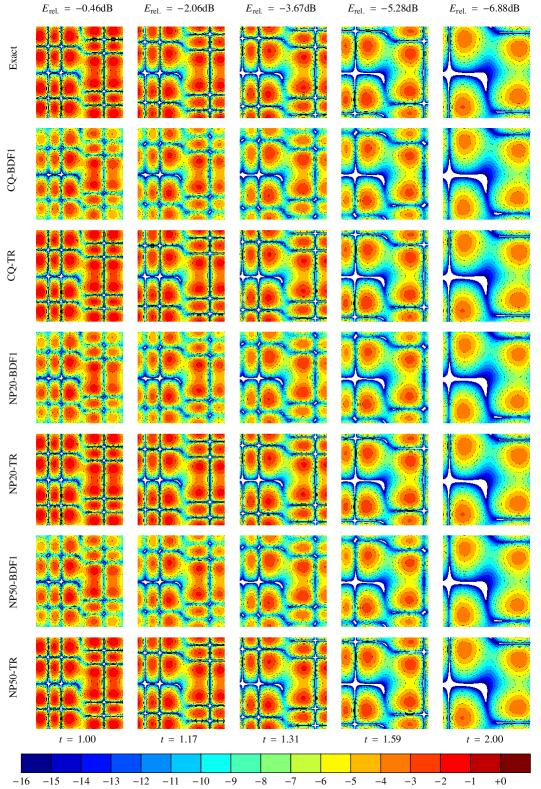
Refer to caption
Figure 13: The figure shows contour plots of 4log10|u(𝒙,t)|4subscript10𝑢𝒙𝑡4\log_{10}|u(\boldsymbol{x},t)| with various TBCs for the chirped-Gaussian profile (see Table 1) for c=12𝑐12c=12 at different instants of time. The numerical parameters and the labels are described in Sec. 4.3.
Refer to caption
Figure 14: The figure shows contour plots of 8log10|u(𝒙,t)|8subscript10𝑢𝒙𝑡8\log_{10}|u(\boldsymbol{x},t)| with various TBCs for the Hermite-Gaussian profile (see Table 2) for c=8𝑐8c=8 at different instants of time. The numerical parameters and the labels are described in Sec. 4.3.

The ideas presented in this paper can be readily extended to three-dimensions. Feschenko and Popov have already shown that the ideas in 2D [4] can be extended to 3D [25]. The formulation of the operator tiΓsubscript𝑡𝑖subscriptΓ\sqrt{\partial_{t}-i\triangle_{\Gamma}} on the boundary of a cuboidal computational domain can be obtained along the same lines as that presented in [5]. For all the cases discussed above, it remains to determine how competitive are PMLs. Such a comparison should however be made for a more general type of Schrödinger equation which is identical to the free Schrödinger on the exterior domain Ωe=dΩ¯i,d=2,3formulae-sequencesubscriptΩ𝑒superscript𝑑subscript¯Ω𝑖𝑑23\Omega_{e}=\mathbb{R}^{d}\setminus\overline{\Omega}_{i},\;d=2,3.

Acknowledgements

The first author thanks CSIR India (grant no. 09/086(1431)/2019-EMR-I) for providing the financial assistance.

References

  • [1] Y. S. Kivshar, G. P. Agrwal, Optical Solitons: From Fibers to Photonic Crystals, 1st Edition, Academic Press, San Diego, California, 2003.
  • [2] D. Lee, S. T. McDaniel, Ocean Acoustic Propagation by Finite Difference Methods, Modern Applied Mathematics and Computer Science, Pergmon Press, New York, 1988.
  • [3] X. Antoine, A. Arnold, C. Besse, M. Ehrhardt, A. Schädle, A review of transparent and artificial boundary conditions techniques for linear and nonlinear Schrödinger equations, Comm. Comput. Phys. 4 (4) (2008) 729–796.
    URL https://hal.archives-ouvertes.fr/hal-00347884
  • [4] R. M. Feshchenko, A. V. Popov, Exact transparent boundary condition for the parabolic equation in a rectangular computational domain, J. Opt. Soc. Am. A 28 (3) (2011) 373–380. doi:10.1364/JOSAA.28.000373.
  • [5] V. Vaibhav, On the nonreflecting boundary operators for the general two dimensional Schrödinger equation, J. Math. Phys. 60 (1) (2019) 011509. doi:10.1063/1.5030875.
  • [6] L. D. Menza, Absorbing boundary conditions on a hypersurface for the Schrödinger equation in a half-space, Appl. Math. Lett. 9 (4) (1996) 55–59. doi:10.1016/0893-9659(96)00051-1.
  • [7] L. D. Menza, Transparent and absorbing boundary conditions for the Schrödinger equation in a bounded domain, Numer. Funct. Anal. Optim. 18 (7) (1997) 759–775. doi:10.1080/01630569708816790.
  • [8] A. Schädle, Non-reflecting boundary conditions for the two-dimensional Schrödinger equation, Wave Motion 35 (2) (2002) 181–188. doi:10.1016/S0165-2125(01)00098-1.
  • [9] H. Han, Z. Huang, Exact artificial boundary conditions for Schrödinger equation in 2superscript2\mathbb{R}^{2}, Comm. Math. Sci. 2 (1) (2004) 79–94.
    URL https://projecteuclid.org/euclid.cms/1250880210
  • [10] S. Ji, Y. Yang, G. Pang, X. Antoine, Accurate artificial boundary conditions for the semi-discretized linear Schrödinger and heat equations on rectangular domains, Comput. Phys. Commun. 222 (2018) 84–93. doi:10.1016/j.cpc.2017.09.019.
  • [11] X. Antoine, C. Besse, P. Klein, Absorbing boundary conditions for the two-dimensional Schrödinger equation with an exterior potential. Part I: Construction and a priori estimates, Math. Models Methods Appl. Sci. 22 (10) (2012) 1250026. doi:10.1142/S0218202512500261.
  • [12] X. Antoine, C. Besse, P. Klein, Absorbing boundary conditions for the two-dimensional Schrödinger equation with an exterior potential. Part II: Discretization and numerical results, Numer. Math. 125 (2) (2013) 191–223. doi:10.1007/S00211-013-0542-8.
  • [13] V. Vaibhav, Microlocal approach towards construction of nonreflecting boundary conditions, J. Comput. Phys. 272 (2014) 588–607. doi:10.1016/j.jcp.2014.04.050.
  • [14] J. Shen, Efficient spectral-Galerkin method i. Direct solvers of second- and fourth-order equations using Legendre polynomials, SIAM J. Sci. Comput. 15 (6) (1994) 1489–1505. doi:10.1137/0915089.
  • [15] C. Lubich, Discretized fractional calculus, SIAM J. Math. Anal. 17 (3) (1986) 704–719. doi:10.1137/0517050.
  • [16] V. Baskakov, A. Popov, Implementation of transparent boundaries for numerical solution of the Schrödinger equation, Wave Motion 14 (2) (1991) 123–128. doi:10.1016/0165-2125(91)90053-Q.
  • [17] B. Mayfield, Nonlocal boundary conditions for the Schrödinger equation, Ph.D. thesis, University of Rhodes Island, Providence, RI (1989).
  • [18] C. Zheng, A perfectly matched layer approach to the nonlinear Schrödinger wave equations, J. Comput. Phys. 227 (1) (2007) 537–556. doi:10.1016/j.jcp.2007.08.004.
  • [19] X. Antoine, C. Geuzaine, Q. Tang, Perfectly matched layer for computing the dynamics of nonlinear schrödinger equations by pseudospectral methods. application to rotating bose-einstein condensates, Communications in Nonlinear Science and Numerical Simulation 90 (2020) 105406. doi:10.1016/j.cnsns.2020.105406.
  • [20] K. Miller, B. Ross, An Introduction to the Fractional Calculus and Fractional Differential Equations, 1st Edition, John Wiley and Sons Inc., 1993.
  • [21] V. Vaibhav, Artificial boundary conditions for certain evolution pdes with cubic nonlinearity for noncompactly supported initial data, J. Comput. Phys. 230 (8) (2011) 3205–3229. doi:10.1016/j.jcp.2011.01.024.
  • [22] S. Yadav, V. Vaibhav, Nonreflecting boundary condition for the free Schrödinger equation in 2d, in: 2023 Photonics and Electromagnetics Research Symposium (PIERS), 2023, pp. 328–337. doi:10.1109/PIERS59004.2023.10221299.
  • [23] N. J. Higham, Accuracy and Stability of Numerical Algorithms, 2nd Edition, Society for Industrial and Applied Mathematics, Philadelphia, 2002. doi:10.1137/1.9780898718027.
  • [24] J. Shen, T. Tang, L. L. Wang, Spectral Methods: Algorithms, Analysis and Applications, 1st Edition, Springer Berlin Heidelberg, 2011.
  • [25] R. M. Feshchenko, A. V. Popov, Exact transparent boundary condition for the three-dimensional Schrödinger equation in a rectangular cuboid computational domain, Phys. Rev. E 88 (2013) 053308. doi:10.1103/PhysRevE.88.053308.

Appendix A Fractional Operators

Definition 1 (Riemann-Liouville fractional integrals).

Let α>0𝛼0\alpha>0 and f(t)𝑓𝑡f(t) be a piecewise continuous function on (0,)0(0,\infty), locally integrable on any finite subinterval of [0,)0[0,\infty). For t>0𝑡0t>0, the Riemann-Liouville fractional integral of order α𝛼\alpha, denoted by tαsuperscriptsubscript𝑡𝛼\partial_{t}^{-\alpha}, is defined by

tαf(t)=1Γ(α)0t(ts)α1f(s)𝑑s.superscriptsubscript𝑡𝛼𝑓𝑡1Γ𝛼subscriptsuperscript𝑡0superscript𝑡𝑠𝛼1𝑓𝑠differential-d𝑠\partial_{t}^{-\alpha}f(t)=\frac{1}{\Gamma(\alpha)}\int^{t}_{0}(t-s)^{\alpha-1}f(s)ds. (187)

where ΓΓ\Gamma denotes the Euler’s Gamma function.

Theorem 1 (Law of exponents).

Let f(t)𝖢([0,))𝑓𝑡superscript𝖢0f(t)\in\mathsf{C}^{\infty}([0,\infty)) and let μ,ν>0𝜇𝜈0\mu,\nu>0, then the composition of two fractional integrals is given by

tν[tμf(t)]=t(μ+ν)f(t)=tμ[tνf(t)],t0.formulae-sequencesuperscriptsubscript𝑡𝜈delimited-[]superscriptsubscript𝑡𝜇𝑓𝑡superscriptsubscript𝑡𝜇𝜈𝑓𝑡superscriptsubscript𝑡𝜇delimited-[]superscriptsubscript𝑡𝜈𝑓𝑡for-all𝑡0\partial_{t}^{-\nu}[\partial_{t}^{-\mu}f(t)]=\partial_{t}^{-(\mu+\nu)}f(t)=\partial_{t}^{-\mu}[\partial_{t}^{-\nu}f(t)],\quad\forall t\geq 0.
Definition 2 (Riemann-Liouville fractional derivatives).

Let f(t)𝖢([0,))𝑓𝑡superscript𝖢0f(t)\in\mathsf{C}^{\infty}([0,\infty)) and let μ>0𝜇0\mu>0. If p𝑝p is the smallest integer greater than μ𝜇\mu, then the fractional derivative of f𝑓f of order μ𝜇\mu is defined by

tμf(t)=tp[tνf(t)],t>0,formulae-sequencesuperscriptsubscript𝑡𝜇𝑓𝑡subscriptsuperscript𝑝𝑡delimited-[]superscriptsubscript𝑡𝜈𝑓𝑡𝑡0\partial_{t}^{\mu}f(t)=\partial^{p}_{t}[\partial_{t}^{-\nu}f(t)],\quad t>0, (188)

where ν=pμ>0𝜈𝑝𝜇0\nu=p-\mu>0. For this fractional derivative to be defined at t=0𝑡0t=0, the function f(t)𝑓𝑡f(t) must have first p1𝑝1p-1 derivatives equal to zero at t=0𝑡0t=0.

Appendix B Boundary Adapted Basis Representation: Useful Results and Identities

In order to leverage the discrete Legendre transforms over Legendre-Gauss-Lobatto nodes, we choose to favour storage of space dependent variables in terms of their Legendre coefficients. As a result of this choice, all operations involving the boundary adapted basis must be implemented via the Legendre transform.

Let us recall the definitions: Ln(y)subscript𝐿𝑛𝑦L_{n}(y) denote the Legendre polynomial of degree n𝑛n and the index set {0,1,,N2}01𝑁2\{0,1,\ldots,N-2\} is denoted by 𝕁𝕁\mathbb{J}. The boundary adapted basis polynomials are given by

ϕp(y)=Lp(y)+bpLp+2(y),bp=κ+12p(p+1)κ+12(p+2)(p+3),p𝕁,formulae-sequencesubscriptitalic-ϕ𝑝𝑦subscript𝐿𝑝𝑦subscript𝑏𝑝subscript𝐿𝑝2𝑦formulae-sequencesubscript𝑏𝑝𝜅12𝑝𝑝1𝜅12𝑝2𝑝3𝑝𝕁\phi_{p}(y)=L_{p}(y)+b_{p}L_{p+2}(y),\quad b_{p}=-\frac{\kappa+\frac{1}{2}p(p+1)}{\kappa+\frac{1}{2}(p+2)(p+3)},\quad p\in\mathbb{J}, (189)

where κ𝜅\kappa\in\mathbb{C}. Let us briefly discuss the parameters that determine this quantity: We recall from Sec. 3.2.1 that β=J2𝛽superscript𝐽2\beta=J^{-2} where J=yx𝐽subscript𝑦𝑥J=\partial_{y}x is the Jacobian corresponding to the transformation from the reference interval 𝕀=[1,1]𝕀11\mathbb{I}=[-1,1] to the actual domain [x,x+]subscript𝑥subscript𝑥[x_{-},x_{+}]. We suppress the subscript which characterizes the axis along which the domain lies for the sake of brevity. The time-stepping schemes discussed in Sec. 3 dictate that either ρ=1/Δt𝜌1Δ𝑡\rho=1/\Delta t (for BDF1) or ρ=2/Δt𝜌2Δ𝑡\rho=2/\Delta t (for TR). The form of κ𝜅\kappa follows from the Robin-type formulation of the discretized version of the DtN-maps as discussed in Sec. 3.1. For CQ methods κ=α=ρ/βexp(iπ/4)𝜅𝛼𝜌𝛽𝑖𝜋4\kappa=\alpha=\sqrt{\rho/\beta}\exp(-i\pi/4) while for the NP methods, we have κ=αϖ𝜅𝛼italic-ϖ\kappa=\alpha\varpi where ϖitalic-ϖ\varpi is defined in (82).

Any arbitrary function in 𝖫2(𝕀)superscript𝖫2𝕀\mathsf{L}^{2}(\mathbb{I}) can be expanded in this basis as follows:

f(y)=p=0N2f^pϕp(y)+η0L0(y)+η1L1(y)=p=0Nf~pLp(y).𝑓𝑦superscriptsubscript𝑝0𝑁2subscript^𝑓𝑝subscriptitalic-ϕ𝑝𝑦subscript𝜂0subscript𝐿0𝑦subscript𝜂1subscript𝐿1𝑦superscriptsubscriptsuperscript𝑝0𝑁subscript~𝑓superscript𝑝subscript𝐿superscript𝑝𝑦f(y)=\sum_{p=0}^{N-2}\hat{f}_{p}\phi_{p}(y)+\eta_{0}L_{0}(y)+\eta_{1}L_{1}(y)=\sum_{p^{\prime}=0}^{N}\tilde{f}_{p^{\prime}}L_{p^{\prime}}(y). (190)

By virtue of linear independence of Legendre polynomials, we can equate their coefficients on both sides of the equality so that

{f~0=f^0+η0,f~1=f^1+η1,f~p=f^p+bp2f^p2,p=2,3,N2,f~N1=bN3f^N3,f~N=bN2f^N2.\left\{\begin{aligned} &\tilde{f}_{0}=\hat{f}_{0}+\eta_{0},\tilde{f}_{1}=\hat{f}_{1}+\eta_{1},\\ &\tilde{f}_{p}=\hat{f}_{p}+b_{p-2}\hat{f}_{p-2},\quad p=2,3,\ldots N-2,\\ &\tilde{f}_{N-1}=b_{N-3}\hat{f}_{N-3},\tilde{f}_{N}=b_{N-2}\hat{f}_{N-2}.\end{aligned}\right. (191)

The linear system can be written as

𝒇~=B𝒇^+η0𝒆0+η1𝒆1~𝒇𝐵^𝒇subscript𝜂0subscript𝒆0subscript𝜂1subscript𝒆1\widetilde{\boldsymbol{f}}=B\widehat{\boldsymbol{f}}+\eta_{0}\boldsymbol{e}_{0}+\eta_{1}\boldsymbol{e}_{1} (192)

where

B=(101b001b101bN401bN30bN2)(N+1)×(N1),𝐵matrix1missing-subexpressionmissing-subexpressionmissing-subexpressionmissing-subexpressionmissing-subexpression01missing-subexpressionmissing-subexpressionmissing-subexpressionmissing-subexpressionsubscript𝑏001missing-subexpressionmissing-subexpressionmissing-subexpressionmissing-subexpressionsubscript𝑏101missing-subexpressionmissing-subexpressionmissing-subexpressionmissing-subexpressionmissing-subexpressionmissing-subexpressionmissing-subexpressionmissing-subexpressionsubscript𝑏𝑁401missing-subexpressionmissing-subexpressionmissing-subexpressionmissing-subexpressionsubscript𝑏𝑁30missing-subexpressionmissing-subexpressionmissing-subexpressionmissing-subexpressionmissing-subexpressionsubscript𝑏𝑁2superscript𝑁1𝑁1B=\begin{pmatrix}1&&&&&\\ 0&1&&&&\\ b_{0}&0&1&&&\\ &b_{1}&0&1&&\\ &&\ddots&\ddots&\ddots&\\ &&&b_{N-4}&0&1\\ &&&&b_{N-3}&0\\ &&&&&b_{N-2}\end{pmatrix}\in\mathbb{C}^{(N+1)\times(N-1)}, (193)

Let the normalization factors be denoted by γk=Lk22=2/(2k+1),k0,formulae-sequencesubscript𝛾𝑘subscriptsuperscriptnormsubscript𝐿𝑘2222𝑘1𝑘subscript0\gamma_{k}=\|L_{k}\|^{2}_{2}=2/(2k+1),\,k\in\mathbb{N}_{0}, and introduce the diagonal matrix Γ=diag(γ0,γ1,,γN)Γdiagsubscript𝛾0subscript𝛾1subscript𝛾𝑁\Gamma=\operatorname{diag}(\gamma_{0},\gamma_{1},\ldots,\gamma_{N}), then inner products of the form gp=(f,ϕp)𝕀,p𝕁,formulae-sequencesubscript𝑔𝑝subscript𝑓subscriptitalic-ϕ𝑝𝕀𝑝𝕁g_{p}=\left(f,\phi_{p}\right)_{\mathbb{I}},\,p\in\mathbb{J}, can be understood as

gp=(f,ϕp)𝕀=[γpf~p+bpγp+2f~p+2],p𝕁.formulae-sequencesubscript𝑔𝑝subscript𝑓subscriptitalic-ϕ𝑝𝕀delimited-[]subscript𝛾𝑝subscript~𝑓𝑝subscript𝑏𝑝subscript𝛾𝑝2subscript~𝑓𝑝2𝑝𝕁g_{p}=\left(f,\phi_{p}\right)_{\mathbb{I}}=\left[\gamma_{p}\tilde{f}_{p}+b_{p}\gamma_{p+2}\tilde{f}_{p+2}\right],\quad p\in\mathbb{J}. (194)

The relationship above can be compactly stated as 𝒈=(g0,g1,,gN2)=QΓ𝒇~𝒈superscriptsubscript𝑔0subscript𝑔1subscript𝑔𝑁2𝑄Γ~𝒇\boldsymbol{g}=(g_{0},g_{1},\ldots,g_{N-2})^{\intercal}=Q\Gamma\widetilde{\boldsymbol{f}} where Q=B𝑄superscript𝐵Q=B^{\intercal} is referred to as the quadrature matrix.

Let the index set {0,1,,N12}01subscript𝑁12\{0,1,\ldots,N_{1}-2\} be denoted by 𝕁1subscript𝕁1\mathbb{J}_{1} and the index set {0,1,,N22}01subscript𝑁22\{0,1,\ldots,N_{2}-2\} be denoted by 𝕁2subscript𝕁2\mathbb{J}_{2}. The boundary adapted basis polynomials are given by

ϕpj(j)(yj)=Lpj(yj)+bpj(j)Lpj+2(yj),pj𝕁j,j=1,2.formulae-sequencesubscriptsuperscriptitalic-ϕ𝑗subscript𝑝𝑗subscript𝑦𝑗subscript𝐿subscript𝑝𝑗subscript𝑦𝑗subscriptsuperscript𝑏𝑗subscript𝑝𝑗subscript𝐿subscript𝑝𝑗2subscript𝑦𝑗formulae-sequencesubscript𝑝𝑗subscript𝕁𝑗𝑗12\phi^{(j)}_{p_{j}}(y_{j})=L_{p_{j}}(y_{j})+b^{(j)}_{p_{j}}L_{p_{j}+2}(y_{j}),\quad p_{j}\in\mathbb{J}_{j},\;j=1,2. (195)

where {bpj(j)}subscriptsuperscript𝑏𝑗subscript𝑝𝑗\{b^{(j)}_{p_{j}}\} is a sequence. Any arbitrary function in 𝖫2(Ωiref)superscript𝖫2superscriptsubscriptΩ𝑖ref\mathsf{L}^{2}(\Omega_{i}^{\text{ref}}) can be expanded in this basis as follows:

f(𝒚)=p1𝕁1p2𝕁2f^p1,p2ϕp1(1)(y1)ϕp2(2)(y2)+p1𝕁1[ζp1,0ϕp1(1)(y1)L0(y2)+ζp1,1ϕp1(1)(y1)L1(y2)]+p2𝕁2[η0,p2L0(y1)ϕp2(2)(y2)+η1,p2L1(y1)ϕp2(2)(y2)]+[κ0,0L0(y1)L0(y2)+κ0,1L0(y1)L1(y2)+κ1,0L1(y1)L0(y2)+κ1,1L1(y1)L1(y2)]=p1=0N1p2=0N2f~p1,p2Lp1(y1)Lp2(y2).𝑓𝒚subscriptsubscript𝑝1subscript𝕁1subscriptsubscript𝑝2subscript𝕁2subscript^𝑓subscript𝑝1subscript𝑝2subscriptsuperscriptitalic-ϕ1subscript𝑝1subscript𝑦1subscriptsuperscriptitalic-ϕ2subscript𝑝2subscript𝑦2subscriptsubscript𝑝1subscript𝕁1delimited-[]subscript𝜁subscript𝑝10subscriptsuperscriptitalic-ϕ1subscript𝑝1subscript𝑦1subscript𝐿0subscript𝑦2subscript𝜁subscript𝑝11subscriptsuperscriptitalic-ϕ1subscript𝑝1subscript𝑦1subscript𝐿1subscript𝑦2subscriptsubscript𝑝2subscript𝕁2delimited-[]subscript𝜂0subscript𝑝2subscript𝐿0subscript𝑦1subscriptsuperscriptitalic-ϕ2subscript𝑝2subscript𝑦2subscript𝜂1subscript𝑝2subscript𝐿1subscript𝑦1subscriptsuperscriptitalic-ϕ2subscript𝑝2subscript𝑦2delimited-[]subscript𝜅00subscript𝐿0subscript𝑦1subscript𝐿0subscript𝑦2subscript𝜅01subscript𝐿0subscript𝑦1subscript𝐿1subscript𝑦2subscript𝜅10subscript𝐿1subscript𝑦1subscript𝐿0subscript𝑦2subscript𝜅11subscript𝐿1subscript𝑦1subscript𝐿1subscript𝑦2superscriptsubscriptsubscript𝑝10subscript𝑁1superscriptsubscriptsubscript𝑝20subscript𝑁2subscript~𝑓subscript𝑝1subscript𝑝2subscript𝐿subscript𝑝1subscript𝑦1subscript𝐿subscript𝑝2subscript𝑦2\begin{split}f(\boldsymbol{y})&=\sum_{p_{1}\in\mathbb{J}_{1}}\sum_{p_{2}\in\mathbb{J}_{2}}\hat{f}_{p_{1},p_{2}}\phi^{(1)}_{p_{1}}(y_{1})\phi^{(2)}_{p_{2}}(y_{2})\\ &\quad+\sum_{p_{1}\in\mathbb{J}_{1}}\left[\zeta_{p_{1},0}\phi^{(1)}_{p_{1}}(y_{1})L_{0}(y_{2})+\zeta_{p_{1},1}\phi^{(1)}_{p_{1}}(y_{1})L_{1}(y_{2})\right]\\ &\quad+\sum_{p_{2}\in\mathbb{J}_{2}}\left[\eta_{0,p_{2}}L_{0}(y_{1})\phi^{(2)}_{p_{2}}(y_{2})+\eta_{1,p_{2}}L_{1}(y_{1})\phi^{(2)}_{p_{2}}(y_{2})\right]\\ &\quad+\left[\kappa_{0,0}L_{0}(y_{1})L_{0}(y_{2})+\kappa_{0,1}L_{0}(y_{1})L_{1}(y_{2})+\kappa_{1,0}L_{1}(y_{1})L_{0}(y_{2})+\kappa_{1,1}L_{1}(y_{1})L_{1}(y_{2})\right]\\ &=\sum_{p_{1}=0}^{N_{1}}\sum_{p_{2}=0}^{N_{2}}\tilde{f}_{p_{1},p_{2}}L_{p_{1}}(y_{1})L_{p_{2}}(y_{2}).\end{split} (196)

For p1=2,3,N12subscript𝑝123subscript𝑁12p_{1}=2,3,\ldots N_{1}-2 and p2=2,3,N22subscript𝑝223subscript𝑁22p_{2}=2,3,\ldots N_{2}-2, equating the coefficients on both sides of equality so that

f~p1,p2=f^p1,p2+bp12(1)f^p12,p2+bp22(2)f^p1,p22+bp12(1)bp22(2)f^p12,p22,subscript~𝑓subscript𝑝1subscript𝑝2subscript^𝑓subscript𝑝1subscript𝑝2subscriptsuperscript𝑏1subscript𝑝12subscript^𝑓subscript𝑝12subscript𝑝2subscriptsuperscript𝑏2subscript𝑝22subscript^𝑓subscript𝑝1subscript𝑝22subscriptsuperscript𝑏1subscript𝑝12subscriptsuperscript𝑏2subscript𝑝22subscript^𝑓subscript𝑝12subscript𝑝22\tilde{f}_{p_{1},p_{2}}=\hat{f}_{p_{1},p_{2}}+b^{(1)}_{p_{1}-2}\hat{f}_{p_{1}-2,p_{2}}+b^{(2)}_{p_{2}-2}\hat{f}_{p_{1},p_{2}-2}+b^{(1)}_{p_{1}-2}b^{(2)}_{p_{2}-2}\hat{f}_{p_{1}-2,p_{2}-2}, (197)

The linear system can be written as

F~=B1F^B2+B1𝜻0(𝒆0(2))+B1𝜻1(𝒆1(2))+𝒆0(1)𝜼0B2+𝒆1(1)𝜼1B2+κ0,0𝒆0(1)(𝒆0(2))+κ0,1𝒆0(1)(𝒆1(2))+κ1,0𝒆1(1)(𝒆0(2))+κ1,1𝒆1(1)(𝒆1(2))~𝐹subscript𝐵1^𝐹superscriptsubscript𝐵2tensor-productsubscript𝐵1subscript𝜻0superscriptsubscriptsuperscript𝒆20tensor-productsubscript𝐵1subscript𝜻1superscriptsubscriptsuperscript𝒆21tensor-productsubscriptsuperscript𝒆10subscript𝜼0superscriptsubscript𝐵2tensor-productsubscriptsuperscript𝒆11subscript𝜼1superscriptsubscript𝐵2tensor-productsubscript𝜅00subscriptsuperscript𝒆10superscriptsubscriptsuperscript𝒆20tensor-productsubscript𝜅01subscriptsuperscript𝒆10superscriptsubscriptsuperscript𝒆21tensor-productsubscript𝜅10subscriptsuperscript𝒆11superscriptsubscriptsuperscript𝒆20tensor-productsubscript𝜅11subscriptsuperscript𝒆11superscriptsubscriptsuperscript𝒆21\begin{split}\widetilde{F}&=B_{1}\widehat{F}B_{2}^{\intercal}+B_{1}\boldsymbol{\zeta}_{0}\otimes\left(\boldsymbol{e}^{(2)}_{0}\right)^{\intercal}+B_{1}\boldsymbol{\zeta}_{1}\otimes\left(\boldsymbol{e}^{(2)}_{1}\right)^{\intercal}+\boldsymbol{e}^{(1)}_{0}\otimes\boldsymbol{\eta}_{0}B_{2}^{\intercal}+\boldsymbol{e}^{(1)}_{1}\otimes\boldsymbol{\eta}_{1}B_{2}^{\intercal}\\ &\quad+\kappa_{0,0}\boldsymbol{e}^{(1)}_{0}\otimes\left(\boldsymbol{e}^{(2)}_{0}\right)^{\intercal}+\kappa_{0,1}\boldsymbol{e}^{(1)}_{0}\otimes\left(\boldsymbol{e}^{(2)}_{1}\right)^{\intercal}+\kappa_{1,0}\boldsymbol{e}^{(1)}_{1}\otimes\left(\boldsymbol{e}^{(2)}_{0}\right)^{\intercal}+\kappa_{1,1}\boldsymbol{e}^{(1)}_{1}\otimes\left(\boldsymbol{e}^{(2)}_{1}\right)^{\intercal}\end{split} (198)

where

Bj=(101b0(j)01b1(j)01bN4(j)01bN3(j)0bN2(j))(N+1)×(N1),subscript𝐵𝑗matrix1missing-subexpressionmissing-subexpressionmissing-subexpressionmissing-subexpressionmissing-subexpression01missing-subexpressionmissing-subexpressionmissing-subexpressionmissing-subexpressionsubscriptsuperscript𝑏𝑗001missing-subexpressionmissing-subexpressionmissing-subexpressionmissing-subexpressionsubscriptsuperscript𝑏𝑗101missing-subexpressionmissing-subexpressionmissing-subexpressionmissing-subexpressionmissing-subexpressionmissing-subexpressionmissing-subexpressionmissing-subexpressionsubscriptsuperscript𝑏𝑗𝑁401missing-subexpressionmissing-subexpressionmissing-subexpressionmissing-subexpressionsubscriptsuperscript𝑏𝑗𝑁30missing-subexpressionmissing-subexpressionmissing-subexpressionmissing-subexpressionmissing-subexpressionsubscriptsuperscript𝑏𝑗𝑁2superscript𝑁1𝑁1B_{j}=\begin{pmatrix}1&&&&&\\ 0&1&&&&\\ b^{(j)}_{0}&0&1&&&\\ &b^{(j)}_{1}&0&1&&\\ &&\ddots&\ddots&\ddots&\\ &&&b^{(j)}_{N-4}&0&1\\ &&&&b^{(j)}_{N-3}&0\\ &&&&&b^{(j)}_{N-2}\end{pmatrix}\in\mathbb{C}^{(N+1)\times(N-1)}, (199)

The inner products of the form gp1,p2=(f,ϕp1(1)ϕp2(2))Ωirefsubscript𝑔subscript𝑝1subscript𝑝2subscript𝑓subscriptsuperscriptitalic-ϕ1subscript𝑝1subscriptsuperscriptitalic-ϕ2subscript𝑝2superscriptsubscriptΩ𝑖refg_{p_{1},p_{2}}=\left(f,\phi^{(1)}_{p_{1}}\phi^{(2)}_{p_{2}}\right)_{\Omega_{i}^{\text{ref}}} can be understood as

gp1,p2=(f,ϕp1(1)ϕp2(2))Ωiref=γp1γp2f~p1,p2+bp1(1)γp1+2γp2f~p1+2,p2+bp2(2)γp1γp2+2f~p1,p2+2+bp1(1)bp2(2)γp1+2γp2+2f~p1+2,p2+2.subscript𝑔subscript𝑝1subscript𝑝2subscript𝑓subscriptsuperscriptitalic-ϕ1subscript𝑝1subscriptsuperscriptitalic-ϕ2subscript𝑝2superscriptsubscriptΩ𝑖refsubscript𝛾subscript𝑝1subscript𝛾subscript𝑝2subscript~𝑓subscript𝑝1subscript𝑝2subscriptsuperscript𝑏1subscript𝑝1subscript𝛾subscript𝑝12subscript𝛾subscript𝑝2subscript~𝑓subscript𝑝12subscript𝑝2subscriptsuperscript𝑏2subscript𝑝2subscript𝛾subscript𝑝1subscript𝛾subscript𝑝22subscript~𝑓subscript𝑝1subscript𝑝22subscriptsuperscript𝑏1subscript𝑝1subscriptsuperscript𝑏2subscript𝑝2subscript𝛾subscript𝑝12subscript𝛾subscript𝑝22subscript~𝑓subscript𝑝12subscript𝑝22\begin{split}g_{p_{1},p_{2}}=\left(f,\phi^{(1)}_{p_{1}}\phi^{(2)}_{p_{2}}\right)_{\Omega_{i}^{\text{ref}}}&=\gamma_{p_{1}}\gamma_{p_{2}}\tilde{f}_{p_{1},p_{2}}+b^{(1)}_{p_{1}}\gamma_{p_{1}+2}\gamma_{p_{2}}\tilde{f}_{p_{1}+2,p_{2}}\\ &\qquad+b^{(2)}_{p_{2}}\gamma_{p_{1}}\gamma_{p_{2}+2}\tilde{f}_{p_{1},p_{2}+2}+b^{(1)}_{p_{1}}b^{(2)}_{p_{2}}\gamma_{p_{1}+2}\gamma_{p_{2}+2}\tilde{f}_{p_{1}+2,p_{2}+2}.\end{split} (200)

The relationship above can be compactly stated as G=(gp1,p2)=Q1ΓF~ΓQ2𝐺subscript𝑔subscript𝑝1subscript𝑝2subscript𝑄1Γ~𝐹Γsuperscriptsubscript𝑄2G=(g_{p_{1},p_{2}})=Q_{1}\Gamma\widetilde{F}\Gamma Q_{2}^{\intercal} where Qj=Bjsubscript𝑄𝑗superscriptsubscript𝐵𝑗Q_{j}=B_{j}^{\intercal} are referred to as the quadrature matrices.