Complete Minimal Left-Right Symmetric Model File

Abstract

We develop a comprehensive implementation of the minimal Left-Right symmetric model within a FeynRules model file. We derive the complete set of mass spectra and mixings for the charged and neutral gauge bosons, would-be-Goldstones and gauge fixing, together with the ghost Lagrangian. In the scalar sector, we analytically re-derive all the massive states with mixings and devise a physical input scheme, which expresses the model couplings in terms of masses and mixing angles of all states. Fermion couplings are determined in closed form, including the Dirac mixing in the neutrino sector, evaluated explicitly with the Cayley-Hamilton method. We calculate the one loop next-to-leading QCD corrections and provide a complete UFO file for NLO studies, demonstrated on relevant benchmarks. We provide various restricted variants of the model file with different gauges, massless states, neutrino hierarchies and parity violating $g_{L}\neq g_{R}$ gauge couplings.

I Introduction

Understanding the microscopic nature of forces and the spontaneous origin of mass are the two core attributes of the Standard Model (SM) [1]. Neutrino oscillations have now firmly established that neutrinos are massive, in contrast to the SM, and recent significant experimental progress determined their mixing properties to unprecedented precision. Still, the nature of neutrino mass (Dirac vs. Majorana) and even more importantly its origin, remain an unsolved mystery of particle physics. Contrary to charged fermions, whose origin is tightly connected to the Higgs mechanism, as the LHC data keeps confirming [2, 3], we do not know which theoretical framework is responsible for neutrino mass generation. Another unsolved puzzle in the SM is the glaring parity asymmetry of weak interactions. With the enduring SM experimental success, we got used to the chiral nature of weak interactions and are taking it for given, but the reason behind it remains as unclear as it was at the time of its discovery.

Left-Right (LR) symmetry addresses both of these shortcomings within a single framework by postulating parity invariance of weak interactions via interchangeable $SU(2)_{L}\times SU(2)_{R}$ local symmetries, featuring new right-handed gauge bosons $W_{R}$ and $Z_{R}$. The need for anomaly cancellation automatically brings in three right-handed neutrinos $N_{i=1,2,3}$, whose mass is tied to the spontaneous breaking scale of $SU(2)_{R}$. Moreover, the $U(1)$ charge assignment becomes very simple and parity symmetric (or vector-like) and is given by $U(1)_{B-L}$.

Gauging lepton number indicates that the Higgs sector may (and in fact does) lead to lepton number violation (LNV), if neutrinos couple to the Higgs with a Majorana-type Yukawa coupling. The original works addressed the issue of parity restoration [4, 5] with soft breaking, but it was soon realized that spontaneous breaking works with both doublets [6] and $\Delta_{L,R}$ triplets [7, 8]. The latter option allows for Majorana mass terms for heavy and light neutrinos, which led to the celebrated seesaw mechanism [9, 10] and features LNV. We shall refer to it as the minimal Left-Right symmetric model (LRSM). In contrast to GUT-inspired seesaw scenarios [11, 12], the LRSM scale need not be much above the electroweak scale, since the interactions do not mediate proton decay.

Indeed, prior to the advent of LHC, the most stringent constraints on the LRSM scale came from flavor physics. The point here is that, as usual in gauge theories, flavor asymmetry comes from the Yukawa sector when the bi-doublet $\phi$ couples to quark doublets $Q_{L,R}$. When LR symmetry, in either $\mathcal{P}$ or $\mathcal{C}$ form, is imposed on the Lagrangian, Yukawa couplings are constrained to be nearly hermitian or symmetric. This implies similar flavor mixings in the quark sector $V^{q}_{R}\sim V^{q}_{L}$ and has led to significant constraints since the Tevatron era [8, 13, 14, 15] that pushed the scale beyond direct detection capabilities of colliders for some time. The increase of center-of-mass energy at the LHC suffices to probe the scales beyond the flavor constraints [16, 17, 18, 19, 20, 21, 22, 23], which spurred a number of collider studies, see reviews in [24, 25, 26, 27].

Arguably the most fundamental signal one can look for is the Keung-Senjanović(KS) [28] production of heavy Majorana neutrinos through $W_{R}$-mediated gauge interactions. With even a tiny amount of data, the recast of leptoquark searches led to a significant bound [29] that was extensively characterized across the $M_{W_{R}}-m_{N}$ plane [30] from well separated $\ell^{\pm}\ell^{\pm}jj$ to boosted neutrino jets [31, 32] with a displaced vertex [30, 33] and finally invisible $N$ [30]. (Some of these bounds are relaxed if CKM is different in left- and right-handed interactions [34, 35, 36].) With enough data it may be possible to characterize the chirality [37, 38], disambiguate production channels [39], look for CP phases in case of degeneracy [40] and include top final states [41]. At even smaller masses, decays of hadrons and mesons become important when a significant amount of decaying states is available [42, 43, 44]. At very high $W_{R}$ masses, off-shell production takes place [45]. Looking into the future, the reach of an FCC-hh was estimated to be around 30 TeV [46], in agreement with other studies [47, 48, 49, 45].

At present, many experimental searches by CMS and ATLAS are targeting $W^{\prime}$ and $Z^{\prime}$ resonances. Here we focus on $W_{R}$, which is lighter than $Z_{R}$ and thus sets the most stringent constraint on the LR breaking scale and we only review the most recent works. The KS channel [50, 51] searches are looking for resolved as well as boosted (but prompt) topologies of $N$ decays. In the low $m_{N}$ regime, the $W_{R}\to\ell N$ channel is equivalent to $W^{\prime}\to\ell\nu$, because $N$ becomes long-lived enough to decay outside of the detector. One can then recast both leptonic ($e,\mu$) [52, 53] as well as $\tau$ final states [54, 55, 56]. In the LR symmetric case, the CKM in the left and right-handed sectors are similar and one has direct limits from dijet [57, 58] and $tb$ resonance [59, 60] searches. The final state topologies here are clearly independent of $m_{N}$ and so is the resulting limit on $M_{W_{R}}$, apart from the slight suppression of the Br when $N$ channels open up. Finally, $W_{R}$ can decay to SM gauge bosons $W,Z$ and Higgs $h$, leading to further dedicated searches [61, 62].

The imposition of LR-symmetry has important ramifications in the leptonic sector, such as $\mu\to e\gamma$, which was the original motivation for seesaw [9]. When the triplet Yukawa couplings are restricted to a near-hermitian or symmetric form, Dirac and Majorana couplings become directly related. In the case of $\mathcal{C}$ [63] this connection allows one to calculate the Dirac mass in terms of Majorana masses, via a square root of a matrix. The analytic solution developed in this work gives a direct insight into the Dirac-Majorana connection from colliders, where Majorana masses may be measured, and connect it to any Dirac-mediated process. These processes appear either at colliders [63, 64, 65, 66], nuclear $0\nu 2\beta$ [10, 67, 68, 69, 70], electron EDMs or radiative decays, and may be relevant for dark matter searches [71, 72, 73]. The connection becomes rather involved in the case of $\mathcal{P}$ [74, 75] and one can resort to numerical algorithms [76] to invert it.

The primary focus of LHC studies has been on the gauge sector, looking for a massive TeV scale $W_{R}$ resonance in the $s$-channel and the associated Majorana neutrino [18, 29, 25, 39, 30]. On the other hand, the Higgs sector is of fundamental importance for experimentally establishing the spontaneous mass origin of heavy neutrinos from $\Delta_{R}$ Yukawa coupling to $N$. The scalar sector was introduced in [6, 7] and analyzed in follow-up studies [77, 78, 79, 80] to the more recent works [81, 82, 83, 84] with emphasis on perturbativity [85, 86, 87], vacuum stability [88, 89, 90] and gravitational waves [91, 92]. Our approach here is to start from physical quantities, masses and mixing angles and use them to compute the potential couplings. We therefore revisit and re-derive the minimization conditions and compute the spectrum to give a closed form solution for the potential parameters in terms of physical inputs.

The most fundamental conceptual goal in the Higgs sector, at least in relation to neutrino mass origin, is to prove the spontaneous origin of the heavy $N$ masses. In this mechanism the decay rate of $\Delta_{R}\to NN$ is proportional to $m_{N}$, which can be measured kinematically, just like $\Gamma_{h\to f\overline{f}}\propto m_{f}^{2}$ in the SM, where $m_{f}$ are alredy known. The two scalars $h$ and $\Delta_{R}$ can mix and we get both $h\to NN$ from the 125 GeV resonance [93] and/or a sizeable production of $\Delta_{R}\to NN$ at the unknown $m_{\Delta}$ [88]. Such signals of Majorana Higgses would finalize the program of determining the origin of neutrino mass and complete the microscopic picture of massive neutrinos.

The rest of the Higgs sector is also conceptually interesting but phenomenologically challenging [85, 84]. The scalar $H$, pseudoscalar $A$ and singly charged $H^{+}$ from the bi-doublet $\phi$ can all mediate FCNCs at tree level and therefore have to be quite above the TeV scale. They are unlikely to be accessible at the LHC but might be visible at future colliders [87]. If $W_{R}$ were light enough to be seen at the LHC, the entire $\Delta_{L}$ would be somewhat split [85] and would appear mainly in cascade decays [94]. The doubly charged $\Delta_{R}^{++}$ may be produced in association with $W_{R}$ [95] and would lead to additional LNV final states [96, 97] or long-lived $\text{d}E/\text{d}x$ signatures [98].

Clearly, there is plenty of rich and conceptually relevant phenomenology to be studied in the context of the LRSM, both at colliders, low energies and in cosmology. To ease such studies it would be desirable to have a complete and consistent implementation of the model file in one place. This is precisely the purpose of this work, where we provide a model file implementation within FeynRules (FR) [99] and related UniversalFeynmanOutput (UFO) versions [100, 101].

We collect and re-derive all the parts of the LRSM, starting from covariant derivatives and gauge eigen-states, together with would-be-Goldstones and ghosts, implementing a switch between the Feynman and unitary gauge. A study of renormalization was performed in the gauge sector [102] and in the Higgs sector [83] at one loop. An earlier tree-level implementation of the LRSM can be found in [103] with arbitrary Yukawa couplings and no mixing in the scalar sector. In the context of seesaw, there are available model files at NLO for type I seesaw/singlets [104], type II [105] and type III [106], as well as effective $W^{\prime}/Z^{\prime}$ model [107, 108] and the Weinberg operator [109].

In this work we pay special attention to the scalar sector and re-derive anew analytic expressions for masses and mixings with a physical input and perturbativity constraints. We take into account the symmetry-imposed flavor structure in the quark sector, leading to symmetric CKM mixings and calculable Yukawa matrices of the extended Higgs sector to fermions. In the neutrino sector we focus in detail on the Majorana-Dirac connection and implement the heavy-light neutrino mixing by devising an explicit closed form solution for the root(s) using the Cayley-Hamilton theorem. This is the first time that a complete and calculable heavy-light neutrino mixing is implemented in a model file, including the current neutrino oscillation data.

Finally, we obtain the QCD one loop counter-terms thus providing, for the first time, the complete LRSM at NLO, which should enhance and simplify future collider studies. We demonstrate the use of the model file on a number of benchmarks that exemplify these developments and quantify, in some cases for the first time, the reduction of uncertainties in LNV signals at the LHC and beyond.

The paper is organized as follows: in section II we introduce the minimal LRSM with the relevant fields. We discuss each of its sectors in a separate sub-section, going from gauge bosons and would-be-Goldstones in II.1 to scalars II.2 (including the inversion of couplings II.3), fermions II.4 and finishing with ghosts in II.5. The section III is dedicated to the variant of the model with different gauge couplings. The core of the implementation of the model file is laid out in IV and the QCD NLO corrections are computed in IV.2. Some phenomenologically relevant benchmarks are given in V, while the summary and outlook is done in VI. The appendix A explains the Cayley-Hamilton approach used to obtain an analytic closed form of the square root of a matrix.

II The minimal Left-Right symmetric model

The minimal Left-Right symmetric model is based on a parity symmetric gauge group

$$G_{LR}=SU(3)_{c}\otimes SU(2)_{L}\otimes SU(2)_{R}\otimes U(1)_{B-L}\,,$$ (1)

where some discrete symmetry interconnects the two $SU(2)_{L,R}$ gauge groups. These two groups are assumed to have the same gauge couplings at some energy scale. We shall be somewhat agnostic about this and first take $g_{L}=g_{R}=g$ for simplicity. Later on we generalize to $g_{L}\neq g_{R}$, which turns out not to be a very drastic change. The gauge coupling of the remaining $U(1)_{B-L}$ is $g^{\prime}$.

In the minimal LRSM, parity and the gauge symmetry are broken spontaneously in the scalar sector, which consists of a bi-doublet $\phi=(\mathbf{1},\mathbf{2},\mathbf{2},\mathbf{0})$ and a pair of triplets $\Delta_{L}=(\mathbf{1},\mathbf{3},\mathbf{1},\mathbf{2})$, $\Delta_{R}=(\mathbf{1},\mathbf{1},\mathbf{3},\mathbf{2})$ under $G_{LR}$. It is convenient to write these fields in the following matrix form

$$\phi =\begin{pmatrix}\phi_{1}^{0*}&\phi_{2}^{+}\\ \phi_{1}^{-}&\phi_{2}^{0}\end{pmatrix}\,, \Delta_{L,R} =\begin{pmatrix}\frac{\Delta^{+}}{\sqrt{2}}&\Delta^{++}\\ \Delta^{0}&-\frac{\Delta^{+}}{\sqrt{2}}\end{pmatrix}_{L,R}\,.$$ (2)

The spontaneous symmetry breaking, which leaves unbroken only the electric charge generator

$$Q=T_{3L}+T_{3R}+\frac{B-L}{2}\,,$$ (3)

follows from the neutral components acquiring the following vevs,

$$\langle\phi\rangle =\begin{pmatrix}v_{1}&0\\ 0&-e^{i\alpha}v_{2}\end{pmatrix}\,, \langle\Delta_{L,R}\rangle =\begin{pmatrix}0&0\\ v_{L,R}&0\end{pmatrix}\,,$$ (4)

where

$$v^{2} =v_{1}^{2}+v_{2}^{2} \tan\beta =\frac{v_{2}}{v_{1}}\,.$$ and (5)

These vevs are quite hierarchical

$$v_{L} \lesssim\text{GeV}\,, v =174\text{ GeV}\,, v_{R}\gtrsim\text{TeV}\,,$$ (6)

and generate the masses of all the states: the gauge and Higgs bosons as well as fermions. The SM-like gauge bosons $W_{L},Z$ are on the order of $v$ and so is the Higgs boson $h$. The RH gauge bosons $W_{R},Z_{LR}$ are heavy, on the order of $v_{R}$ and so are most of the remaining scalars in $\Delta_{L,R}$ and the mass eigenstates $H,A,H^{\pm}$ from the bi-doublet. Of course, the photon remains massless, while the Goldstones are initially massless and then get their unphysical masses from gauge fixing.

The fermions come in LR symmetric doublet representations

$$Q_{L,R} =\begin{pmatrix}u\\ d\end{pmatrix}_{L,R}\,, L_{L,R} =\begin{pmatrix}\nu\\ \ell\end{pmatrix}_{L,R}\,,$$ (7)

with the usual three family copies. The appealing feature of this setup is that the three RH neutrinos $\nu_{R}$ are required by anomaly cancellation. In the LRSM, all the fermion masses come from spontaneous breaking of the two $SU(2)$ groups, meaning their masses are a product of Yukawa couplings and vevs. For $O(1)$ Yukawa couplings, the Dirac masses are on the order of $v$, only the Majorana mass for $\nu_{R}$ is $\mathcal{O}(v_{R})$, while the $\nu_{L}$ may have a Majorana mass on the order of $v_{L}$.

In the following section II.1 we compute the gauge boson masses and mixings and derive the required gauge fixing terms. Then we focus on the scalar sector, which includes the Goldstones and the physical states. We shall calculate the mass spectra, define an input scheme and compute the parameters of the potential in terms of masses and mixings.

II.1 Gauge sector

Gauge boson masses and mixings. Let us begin with the calculation of the gauge boson mass spectrum in the LRSM. The canonical kinetic terms for complex scalar fields are

$$\mathcal{L}_{\text{kin}} =\left|D\phi\right|^{2}+\left|D\Delta_{L}\right|^{2}+\left|D\Delta_{R}\right|^{2}\,,$$ (8)

with

$$D\phi =\partial\phi-ig\left(A_{L}\phi-\phi A_{R}\right)\,,$$ (9)

$$D\Delta_{i} =\partial\Delta_{i}-ig\left[A_{i},\Delta_{i}\right]-ig^{\prime}B\Delta_{i}\,,$$ (10)

where $i=L,R$ and the gauge group and Lorentz indices are suppressed. The gauge bosons states in the flavor basis are

$$A_{i} =A_{i}^{a}\frac{\sigma^{a}}{2}\,, A_{i}^{\pm} =\frac{A^{1}_{i}\mp iA^{2}_{i}}{\sqrt{2}}\,,$$ (11)

where the sum over the repeated $a=1,2,3$ indices is implied.

The signs of the gauge coupling terms in the covariant derivatives of (8) and (10) are not uniquely defined, as is the case for the SM [110]. The convention above is chosen to match the SM-like decoupling limit, such that when $\tan\beta\to 0$, the $\phi_{1}$ takes on the role of the SM Higgs and has the usual covariant derivative. One also has to keep a consistent choice of signs between the bi-doublet $\phi$ and $\Delta_{R}$. None of these considerations affect the gauge boson mass calculation, they only come into play when we consider the gauge fixing that has to remove the mixed generic $V\partial\phi$ terms.

Gauge boson masses and mixings. Covariant derivatives in (8) and (10) generate the gauge boson mass matrices for charged and neutral gauge bosons

$$\begin{split}&\begin{pmatrix}A_{L}^{-}&A_{R}^{-}\end{pmatrix}M_{W_{LR}}^{2}\begin{pmatrix}A_{L}^{+}\\ A_{R}^{+}\end{pmatrix}=\\ &\quad=\begin{pmatrix}W_{L}^{-}&W_{R}^{-}\end{pmatrix}\begin{pmatrix}M_{W_{L}}^{2}&0\\ 0&M_{W_{R}}^{2}\end{pmatrix}\begin{pmatrix}W_{L}^{+}\\ W_{R}^{+}\end{pmatrix}\,.\end{split}$$ (12)

The hermitian mass matrix $M_{W_{LR}}^{2}$ is defined in the gauge basis

$$M_{W_{LR}}^{2} =\frac{g^{2}}{2}v_{R}^{2}\begin{pmatrix}\epsilon^{2}&e^{-i\alpha}\epsilon^{2}s_{2\beta}\\[4.30554pt] e^{i\alpha}\epsilon^{2}s_{2\beta}&2+\epsilon^{2}\end{pmatrix}\,,$$ (13)

where we introduced the dimensionless ratio of vevs

$$\epsilon =\frac{v}{v_{R}}\,,$$ (14)

which needs to be small on phenomenological grounds.

We compute the eigenvalues and expand them in $\epsilon$

$$M_{W_{L}} \simeq\frac{gv}{\sqrt{2}}\,, M_{W_{R}} \simeq gv_{R}\left(1+\frac{\epsilon^{2}}{4}\right)\,,$$ (15)

with the short-hands $s_{x}=\sin(x),c_{x}=\cos(x)$ and $t_{x}=\tan(x)$. We drop higher order corrections of the order of $\epsilon^{4}$ in both the $M_{W_{L}}^{2}$ and $M_{W_{R}}^{2}$. Specifically, the $\epsilon^{2}$ term in $M_{W_{R}}^{2}$ is of the same order as $M_{W_{L}}^{2}$.

To get from the gauge/flavor to the mass basis

$$\begin{pmatrix}A_{L}^{+}\\ A_{R}^{+}\end{pmatrix} =U_{W}\begin{pmatrix}W_{L}^{+}\\ W_{R}^{+}\end{pmatrix}\,,$$ (16)

we have the following $2D$ unitary rotation matrix

$$U_{W} =\begin{pmatrix}c_{\xi}&s_{\xi}e^{-i\alpha}\\[4.30554pt] -s_{\xi}e^{i\alpha}&c_{\xi}\end{pmatrix}\,,$$ (17)

with the mixing angle given by

$$s_{\xi} \simeq\frac{\epsilon^{2}}{2}s_{2\beta}\simeq\frac{M_{W_{L}}^{2}}{M_{W_{R}}^{2}}s_{2\beta}\,.$$ (18)

The $W^{-}$ states get rotated with $U_{W}^{*}$, such that

$$U_{W}^{\dagger}M_{W_{LR}}^{2}U_{W} =\begin{pmatrix}M_{W_{L}}^{2}&0\\ 0&M_{W_{R}}^{2}\end{pmatrix}\,.$$ (19)

We move on to neutral gauge bosons between the following bases

$$\begin{split}&\begin{pmatrix}A_{3L}&A_{3R}&B\end{pmatrix}M_{Z_{LR}}^{2}\begin{pmatrix}A_{3L}\\ A_{3R}\\ B\end{pmatrix}=\\ &\quad=\begin{pmatrix}A&Z_{L}&Z_{R}\end{pmatrix}\begin{pmatrix}0&0&0\\ 0&M_{Z}^{2}&0\\ 0&0&M_{Z_{LR}}^{2}\end{pmatrix}\begin{pmatrix}A\\ Z_{L}\\ Z_{R}\end{pmatrix}\,,\end{split}$$ (20)

where the symmetric mass matrix in the gauge basis is given by

$$M_{Z_{LR}}^{2} =\frac{g^{2}}{2}v_{R}^{2}\begin{pmatrix}\epsilon^{2}&-\epsilon^{2}&0\\ -\epsilon^{2}&4+\epsilon^{2}&-4r\\ 0&-4r&4r^{2}\end{pmatrix}\,, r =\frac{g^{\prime}}{g}\,.$$ (21)

This is a real matrix (no CP phases) that does not depend on $t_{\beta}$, and its eigenvalues can be expanded in $\epsilon$

$$M_{A} =0\,,\qquad\,M_{Z}\simeq\frac{gv}{\sqrt{1+\frac{1}{1+2r^{2}}}}\,,$$ (22)

$$M_{Z_{LR}} \simeq gv_{R}\sqrt{2(1+r^{2})}\left(1+\frac{\epsilon^{2}}{8\left(1+r^{2}\right)^{2}}\right)\,.$$ (23)

One way to define the weak mixing angle is through the ratio of gauge boson masses at leading order in $\epsilon$

$$c_{w} =\frac{M_{W_{L}}}{M_{Z_{L}}}\biggr{|}_{\mathcal{O}(\epsilon^{0})}\,,$$ (24)

which in turn determines the ratio

$$r =\frac{s_{w}}{\sqrt{c_{2w}}}\simeq\sqrt{\frac{M_{W_{L}}^{2}}{2M_{W_{L}}^{2}-M_{Z_{L}}^{2}}-1}\simeq 0.63\,.$$ (25)

From (23) one then recovers the prediction

$$\frac{M_{Z_{LR}}}{M_{W_{R}}} \simeq\sqrt{\frac{2c_{w}^{2}}{c_{2w}}}\left(1+\frac{\epsilon^{2}}{8}\frac{c_{2w}^{2}}{c_{w}^{4}}\right)\simeq 1.67\,.$$ (26)

With these definitions, the real orthogonal matrix $O_{Z}$ that takes us from the flavor to the mass basis,

$$\begin{pmatrix}A_{3L}\\ A_{3R}\\ B\end{pmatrix} =O_{Z}\begin{pmatrix}A\\ Z_{L}\\ Z_{R}\end{pmatrix}\,,$$ (27)

is found at second order in $\epsilon$ to be

$$O_{Z}= \begin{pmatrix}s_{w}&-c_{w}&0\\ s_{w}&s_{w}t_{w}&\!\!-\frac{\sqrt{c_{2w}}}{c_{w}}\\ \sqrt{c_{2w}}&\sqrt{c_{2w}}t_{w}&t_{w}\end{pmatrix}$$

$$+\frac{\epsilon^{2}}{4}\begin{pmatrix}0&0&\frac{c_{2w}^{3/2}}{c_{w}^{3}}\\ 0&-\frac{c_{2w}^{2}}{c_{w}^{5}}&-\frac{c_{2w}^{3/2}t_{w}^{2}}{c_{w}^{3}}\\ 0&\frac{c_{2w}^{3/2}t_{w}}{c_{w}^{4}}&-\frac{c_{2w}^{2}t_{w}}{c_{w}^{4}}\end{pmatrix}\,.$$ (28)

This concludes the analysis of the gauge boson spectrum.

Goldstones and gauge fixing. To complete the description of massive gauge bosons with spontaneous symmetry breaking, we need to address the would-be-Goldstone (wbG) boson sector. Prior to gauge fixing, these appear as massless states of the scalar mass matrices. In the SM there is only one neutral and one charged wbG, however in theories with an extended scalar sector, like the LRSM, there are more such states and they typically mix. Thus we get degenerate zeroes and additional freedom of rotation between massless states.

In the case of the LRSM, we are dealing with two charged wbG modes for the $W_{L,R}$ and two neutral ones for $Z,Z_{LR}$ gauge bosons, thus this freedom comes as one mixing angle for each sector. These angles are not arbitrary, because the proper wbG mode has to couple derivatively and in proportion to the corresponding gauge boson mass, i.e. $M_{V}(V\partial\phi)$. In other words, one needs to isolate the proper wbG mode for each gauge boson. Eventually, we will add the gauge fixing terms in the mass basis, which cancel the derivative mixed terms and generate the usual gauge dependent propagators for vectors and wbGs.

We discuss first the singly charged states and derive their mass matrix. It comes from the mixed second derivatives of the potential $\text{d}^{2}V/(\text{d}\phi_{i}^{+}\text{d}\phi_{j}^{-})$, evaluated at its minimum. The minimization is described in the scalar sector section below. We use the following basis

$$\begin{split}&\begin{pmatrix}\phi_{1}^{-}&\phi_{2}^{-}&\Delta_{R}^{-}\end{pmatrix}M_{+}^{2}\begin{pmatrix}\phi_{1}^{+}\\ \phi_{2}^{+}\\ \Delta_{R}^{+}\end{pmatrix}=\\ &\quad=\begin{pmatrix}\varphi_{L}^{-}&H^{-}&\varphi_{R}^{-}\end{pmatrix}\begin{pmatrix}0&0&0\\ 0&m_{H^{+}}^{2}&0\\ 0&0&0\end{pmatrix}\begin{pmatrix}\varphi_{L}^{+}\\ H^{+}\\ \varphi_{R}^{+}\end{pmatrix},\end{split}$$ (29)

where we dropped the $\Delta_{L}^{\pm}$, because of the negligible $v_{L}$.

The singly charged mass matrix and its only nonzero eigenvalue are given by

$$M_{+}^{2} =\alpha_{3}v_{R}^{2}\begin{pmatrix}\frac{s_{\beta}^{2}}{c_{2\beta}}&-e^{-i\alpha}\frac{t_{2\beta}}{2}&-\epsilon e^{-i\alpha}\frac{s_{\beta}}{\sqrt{2}}\\[4.30554pt] -e^{i\alpha}\frac{t_{2\beta}}{2}&\frac{c_{\beta}^{2}}{c_{2\beta}}&\epsilon\frac{c_{\beta}}{\sqrt{2}}\\[8.61108pt] -\epsilon e^{i\alpha}\frac{s_{\beta}}{\sqrt{2}}&\epsilon\frac{c_{\beta}}{\sqrt{2}}&\epsilon^{2}\frac{c_{2\beta}}{2}\end{pmatrix}\,,$$ (30)

$$m_{H^{+}} \simeq\sqrt{\frac{\alpha_{3}}{c_{2\beta}}}v_{R}\left(1+\epsilon^{2}\frac{c_{2\beta}^{3/2}}{4}\right)\,.$$ (31)

As expected, there are two zero modes in (LABEL:eq:Mp2Def) that are eaten up by the SM-like $W_{L}$ and the new $W_{R}$.

One could diagonalize $M_{+}^{2}$ in (30) by two subsequent rotations. However, this is not enough: after this diagonalization and after performing the $U_{W}$ rotation among $W_{L,R}$, the mixed derivative terms, coming from (8) and (10), are still off-diagonal. In particular, while both $W_{L,R}^{-}\partial H^{+}$ terms vanish as they should, the other four combinations $W_{L,R}^{-}\partial\varphi_{L,R}^{+}$ between incompletely rotated $\varphi^{+}_{L,R}$ are all there. We need to perform one final rotation between wbGs to get rid off the two off-diagonal terms, which finally extracts the canonical would-be-Goldstone modes.

Combining all the rotations, we get the complete transformation of the charged scalars

$$\begin{pmatrix}\phi_{1}^{+}\\ \phi_{2}^{+}\\ \Delta_{R}^{+}\end{pmatrix}=U_{+}\,\begin{pmatrix}\varphi_{L}^{+}\\ H^{+}\\ \varphi_{R}^{+}\end{pmatrix},$$ (32)

where the unitary matrix $U_{+}$ is given by three subsequent rotations and can also be expanded in $\epsilon$,

$$\begin{split}U_{+}&=\begin{pmatrix}c_{\beta}&-e^{-i\alpha}s_{\beta}&0\\ e^{i\alpha}s_{\beta}&c_{\beta}&0\\ 0&0&1\end{pmatrix}\begin{pmatrix}1&0&0\\ 0&-1+\frac{1}{4}\epsilon^{2}c_{2\beta}^{2}&\frac{\epsilon c_{2\beta}}{\sqrt{2}}\\ 0&-\frac{\epsilon c_{2\beta}}{\sqrt{2}}&-1+\frac{1}{4}\epsilon^{2}c_{2\beta}^{2}\end{pmatrix}\begin{pmatrix}1-\frac{1}{4}\epsilon^{2}s_{2\beta}^{2}&0&\frac{\epsilon s_{2\beta}}{\sqrt{2}}\\ 0&1&0\\ -\frac{\epsilon s_{2\beta}}{\sqrt{2}}&0&1-\frac{1}{4}\epsilon^{2}s_{2\beta}^{2}\end{pmatrix}\\[4.30554pt] &\simeq\begin{pmatrix}c_{\beta}&e^{-i\alpha}s_{\beta}&0\\ e^{i\alpha}s_{\beta}&-c_{\beta}&0\\ 0&0&-1\end{pmatrix}+\frac{\epsilon}{\sqrt{2}}\begin{pmatrix}0&0&e^{-i\alpha}s_{\beta}\\ 0&0&c_{\beta}\\ e^{i\alpha}s_{2\beta}&-c_{2\beta}&0\end{pmatrix}+\frac{\epsilon^{2}}{2}\begin{pmatrix}-4c_{\beta}s_{\beta}^{4}&-e^{-i\alpha}s_{\beta}c_{2\beta}^{2}&0\\ -4e^{i\alpha}s_{\beta}c_{\beta}^{4}&c_{\beta}c_{2\beta}^{2}&0\\ 0&0&1\end{pmatrix}\,,\end{split}$$ (33)

which is unitary up to $\mathcal{O}(\epsilon^{2})$.

After performing all the rotations with $U_{W}$ and $U_{+}$, we end up with canonical wbGs that have derivative couplings proportional to the corresponding gauge boson masses

$$\mathcal{L}_{\text{kin}}\ni-i\sum_{i=L,R}M_{W_{i}}W_{i}^{-}\partial\varphi_{i}^{+}\,.$$ (34)

The final step is to add the gauge fixing terms, which come in the usual form, written in the mass basis

$$\mathcal{L}_{\text{gf}} \ni-\sum_{i=L,R}\frac{1}{\xi_{W_{i}}}F_{i}^{+}F_{i}^{-}\,,$$ (35)

$$F_{i}^{+} =\partial W_{i}^{+}+i\xi_{W_{i}}M_{W_{i}}\varphi^{+}_{i}\,.$$ (36)

After expanding all the terms in $\mathcal{L}_{\text{gf}}$ and integrating by parts, the mixed $V\partial\varphi$ terms in (34) cancel away. The remaining terms in (35) give the standard $R_{\xi}$ propagators for the $W$’s and wbGs.

In the neutral sector, the procedure of setting up the wbG rotations and fixing the gauge goes along the same lines. The major additional complication is that there are more neutral states that mix and computing their eigenvalues and mixings becomes a bit more tedious. However, it is fairly simple to isolate the wbG modes away from the massive scalars and complete all the rotations in the gauge-wbG sector. The following field substitution in (2) gets the job done

$$\phi_{10} =v_{1}+\frac{1}{\sqrt{2}}\left(c_{\beta}\varphi_{10}+s_{\beta}e^{-i\alpha}\varphi_{20}\right)\,,$$ (37)

$$\phi_{20} =-v_{2}e^{i\alpha}+\frac{1}{\sqrt{2}}\left(c_{\beta}\varphi_{20}-s_{\beta}e^{i\alpha}\varphi_{10}\right)\,.$$ (38)

With this rotation, the $\Im(\varphi_{10})$ and $\Im(\Delta_{R}^{0})$ decouple from the other neutral scalars and they both have a zero eigenvalue. However, their derivative couplings are still off-diagonal, so we need to perform one final $2D$ rotation to get to the diagonal neutral wbG states

$$\begin{pmatrix}\Im(\varphi_{10})\\ \Im(\Delta_{R}^{0})\end{pmatrix} =O_{\varphi}\begin{pmatrix}\varphi_{L}^{0}\\ \varphi_{R}^{0}\end{pmatrix}\,,$$ (39)

$$O_{\varphi} =I_{2}-\frac{i\sigma_{2}}{2\left(1+r^{2}\right)}\epsilon-\frac{I_{2}}{8\left(1+r^{2}\right)^{2}}\epsilon^{2}\,.$$ (40)

Here, $I_{2}$ is the 2D identity matrix and $\sigma_{2}$ is the usual Pauli matrix. The resulting mixed derivative terms are now diagonal and proportional to the neutral gauge boson masses

$$\mathcal{L}_{\text{kin}}\ni-\sum_{i=L,R}M_{Z_{i}}Z_{i}\partial\varphi_{i}^{0}\,.$$ (41)

Again, they get cancelled by the terms that complete the gauge fixing

$$\mathcal{L}_{\text{gf}} \ni-\sum_{i=L,R}\frac{1}{2\xi_{Z_{i}}}F_{Z_{i}}^{2}\,, F_{Z_{i}} =\partial Z_{i}+\xi_{Z_{i}}M_{Z_{i}}\varphi^{0}_{i}\,,$$ (42)

which also give the canonical $R_{\xi}$ propagators for the neutral gauge bosons and wbGs.

II.2 Scalar sector

The scalar potential of the LRSM comprises all possible bi-linear and quartic terms of the scalar fields, obeying the gauge symmetry, and one discrete LR symmetry, either $\mathcal{P}$ or $\mathcal{C}$:

$$\mathcal{V} =-\mu_{1}^{2}\left[\phi^{\dagger}\phi\right]-\mu_{2}^{2}\left(\left[\tilde{\phi}\phi^{\dagger}\right]+\left[\tilde{\phi}^{\dagger}\phi\right]\right)-\mu_{3}^{2}\left(\left[\Delta_{L}^{{\color[rgb]{1,1,1}\dagger}}\Delta_{L}^{\dagger}\right]+\left[\Delta_{R}^{{\color[rgb]{1,1,1}\dagger}}\Delta_{R}^{\dagger}\right]\right)$$

$$+\lambda_{1}\left[\phi^{\dagger}\phi\right]^{2}+\lambda_{2}\left(\left[\tilde{\phi}\phi^{\dagger}\right]^{2}+\left[\tilde{\phi}^{\dagger}\phi\right]^{2}\right)+\lambda_{3}\left[\tilde{\phi}\phi^{\dagger}\right]\left[\tilde{\phi}^{\dagger}\phi\right]+\lambda_{4}\left[\phi^{\dagger}\phi\right]\left(\left[\tilde{\phi}\phi^{\dagger}\right]+\left[\tilde{\phi}^{\dagger}\phi\right]\right)$$

$$+\rho_{1}\left(\left[\Delta_{L}^{{\color[rgb]{1,1,1}\dagger}}\Delta_{L}^{\dagger}\right]^{2}+\left[\Delta_{R}^{{\color[rgb]{1,1,1}\dagger}}\Delta_{R}^{\dagger}\right]^{2}\right)+\rho_{2}\left(\left[\Delta_{L}^{{\color[rgb]{1,1,1}\dagger}}\Delta_{L}^{{\color[rgb]{1,1,1}\dagger}}\right]\left[\Delta_{L}^{\dagger}\Delta_{L}^{\dagger}\right]+\left[\Delta_{R}^{{\color[rgb]{1,1,1}\dagger}}\Delta_{R}^{{\color[rgb]{1,1,1}\dagger}}\right]\left[\Delta_{R}^{\dagger}\Delta_{R}^{\dagger}\right]\right)+\rho_{3}\left[\Delta_{L}^{{\color[rgb]{1,1,1}\dagger}}\Delta_{L}^{\dagger}\right]\left[\Delta_{R}^{{\color[rgb]{1,1,1}\dagger}}\Delta_{R}^{\dagger}\right]$$

$$+\rho_{4}\left(\left[\Delta_{L}^{{\color[rgb]{1,1,1}\dagger}}\Delta_{L}^{{\color[rgb]{1,1,1}\dagger}}\right]\left[\Delta_{R}^{\dagger}\Delta_{R}^{\dagger}\right]+\left[\Delta_{L}^{\dagger}\Delta_{L}^{\dagger}\right]\left[\Delta_{R}^{{\color[rgb]{1,1,1}\dagger}}\Delta_{R}^{{\color[rgb]{1,1,1}\dagger}}\right]\right)+\alpha_{1}\left[\phi^{\dagger}\phi\right]\left(\left[\Delta_{L}^{{\color[rgb]{1,1,1}\dagger}}\Delta_{L}^{\dagger}\right]+\left[\Delta_{R}^{{\color[rgb]{1,1,1}\dagger}}\Delta_{R}^{\dagger}\right]\right)$$ (43)

$$+\left(\alpha_{2}\left(\left[\tilde{\phi}\phi^{\dagger}\right]\left[\Delta_{L}^{{\color[rgb]{1,1,1}\dagger}}\Delta_{L}^{\dagger}\right]+\left[\tilde{\phi}^{\dagger}\phi\right]\left[\Delta_{R}^{{\color[rgb]{1,1,1}\dagger}}\Delta_{R}^{\dagger}\right]\right)+\text{h.c.}\right)+\alpha_{3}\left(\left[\phi\phi^{\dagger}\Delta_{L}^{{\color[rgb]{1,1,1}\dagger}}\Delta_{L}^{\dagger}\right]+\left[\phi^{\dagger}\phi\Delta_{R}^{{\color[rgb]{1,1,1}\dagger}}\Delta_{R}^{\dagger}\right]\right)$$

$$+\beta_{1}\left(\left[\phi\Delta_{R}^{{\color[rgb]{1,1,1}\dagger}}\phi^{\dagger}\Delta_{L}^{\dagger}\right]+\left[\phi^{\dagger}\Delta_{L}^{{\color[rgb]{1,1,1}\dagger}}\phi\Delta_{R}^{\dagger}\right]\right)+\beta_{2}\left(\left[\tilde{\phi}\Delta_{R}^{{\color[rgb]{1,1,1}\dagger}}\phi^{\dagger}\Delta_{L}^{\dagger}\right]+\left[\tilde{\phi}^{\dagger}\Delta_{L}^{{\color[rgb]{1,1,1}\dagger}}\phi\Delta_{R}^{\dagger}\right]\right)+\beta_{3}\left(\left[\phi\Delta_{R}^{{\color[rgb]{1,1,1}\dagger}}\tilde{\phi}^{\dagger}\Delta_{L}^{\dagger}\right]+\left[\phi^{\dagger}\Delta_{L}^{{\color[rgb]{1,1,1}\dagger}}\tilde{\phi}\Delta_{R}^{\dagger}\right]\right),$$

where $\tilde{\phi}=\sigma_{2}\phi^{*}\sigma_{2}$ and the square brackets imply the trace over field components. In the following, we set for simplicity $\beta_{i}\simeq 0$, which sets $v_{L}=0$ and remains small; this is a technically natural assumption.

The $\mathcal{P}$ or $\mathcal{C}$ discrete symmetries further constrain the coupling constants.

The case of $\mathcal{P}$.

With this choice, the scalars transform as

$$\mathcal{P} :\phi\to\phi^{\dagger}\,, \Delta_{L} \leftrightarrow\Delta_{R}\,,$$ (44)

and all the couplings in the potential must be real except for $\alpha_{2}$, which carries a phase ${\rm e}^{i\delta_{2}}$.

The minimization conditions can be interpreted as determining the $\mu_{i}$ in terms of the vevs and quartic couplings:

$$\mu_{1}^{2}= 2\left(\lambda_{1}+s_{2\beta}c_{\alpha}\lambda_{4}\right)v^{2}+\left(\alpha_{1}-\alpha_{3}\frac{s_{\beta}^{2}}{c_{2\beta}}\right)v_{R}^{2}\,,$$ (45)

$$\mu_{2}^{2}= \left(s_{2\beta}\left(2c_{2\alpha}\lambda_{2}+\lambda_{3}\right)+\lambda_{4}\right)v^{2}$$

$${}+\frac{1}{2c_{\alpha}}\left(2c_{\alpha+\delta_{2}}\alpha_{2}+\alpha_{3}\frac{t_{2\beta}}{2c_{\alpha}}\right)v_{R}^{2}\,,$$ (46)

$$\mu_{3}^{2}= \left(\alpha_{1}+\left(2c_{\alpha+\delta_{2}}\alpha_{2}s_{2\beta}+\alpha_{3}s_{\beta}^{2}\right)\right)v^{2}+2\rho_{1}v_{R}^{2}\,.$$ (47)

where $v_{L}$ is neglected, since $v_{L}\ll v\ll v_{R}$. In fact, one has

$$\begin{split}v_{L}=&\frac{\epsilon^{2}v_{R}}{\left(1+t_{\beta}^{2}\right)\left(2\rho_{1}-\rho_{3}\right)}\biggl{(}-\beta_{1}t_{\beta}\cos(\alpha-\theta_{L})\\ &+\beta_{2}\cos(\theta_{L})+\beta_{3}t_{\beta}^{2}\cos(2\alpha-\theta_{L})\biggr{)}\,.\end{split}$$ (48)

The derivative with respect to $\alpha$ connects it to the only CP phase $\delta_{2}$:

$$\alpha_{2}s_{\delta_{2}} =\frac{s_{\alpha}}{4}\left(\alpha_{3}t_{2\beta}+4\left(\lambda_{3}-2\lambda_{2}\right)s_{2\beta}\epsilon^{2}\right).$$ (49)

The case of $\mathcal{C}$.

This acts as

$$\mathcal{C}:\phi\to\phi^{T}\,,\qquad\Delta_{L}\leftrightarrow\Delta_{R}^{*}\,.$$ (50)

This choice allows for additional complex phases in the potential. In particular, the couplings $\mu_{2}$, $\lambda_{2}$, $\lambda_{4}$, $\rho_{4}$ and $\beta_{i}$ are now complex, introducing seven new CP violating phases. The minimization conditions described above also change accordingly.

However, for collider studies, these additional phases do not lead to relevant new features, while spoiling the exact solvability of the scalar spectrum that we achieve below. Therefore, in the present work we retain the single CP phase $\delta_{2}$ as in the case of $\mathcal{P}$. Similarly, we can consider the limit of vanishing $v_{L}$, and accordingly we set $\beta_{i}\to 0$.

II.2.1 Doubly charged $\Delta_{R}^{++}$ and the entire $\Delta_{L}$ triplet

In the $v_{L}\to 0$ limit, the doubly charged $\Delta_{R}^{++}$ and $\Delta_{L}$ triplet of states do not mix with other scalars, and their mass matrix is diagonal to begin with. The simplest is

$$m_{\Delta_{R}^{++}}^{2} =v_{R}^{2}\left(4\rho_{2}+\frac{c_{2\beta}}{c_{\beta}^{4}}\alpha_{3}\epsilon^{2}\right)\,,$$ (51)

and the $\Delta_{L}$ triplet masses are given by

$$m_{\Delta_{L}^{0}}^{2} =v_{R}^{2}\bigg{[}\rho_{3}-2\rho_{1}+\epsilon^{2}\alpha_{3}\,s_{2\beta}t_{2\beta}\,s^{2}_{\alpha}\bigg{]}=m_{\chi_{L}^{0}}^{2}\,,$$ (52)

$$m_{\Delta_{L}^{+}}^{2} =v_{R}^{2}\bigg{[}\rho_{3}-2\rho_{1}+\epsilon^{2}\alpha_{3}\left(s_{2\beta}t_{2\beta}\,s^{2}_{\alpha}+\frac{c_{2\beta}}{2}\right)\bigg{]}\,,$$ (53)

$$m_{\Delta_{L}^{++}}^{2}\! =v_{R}^{2}\bigg{[}\rho_{3}-2\rho_{1}+\epsilon^{2}\alpha_{3}\left(s_{2\beta}t_{2\beta}\,s^{2}_{\alpha}+c_{2\beta}\right)\bigg{]}\,,$$ (54)

where clearly the four states within the $\Delta_{L}$ triplet are degenerate up to $\epsilon^{2}$ corrections. These relations can be readily solved for e.g. $\rho_{2}$ and $\rho_{3}$ in terms of two masses, $m_{\Delta_{R}^{++}}$, $m_{\Delta_{L}}$, as we do below. The remaining three masses within the $\Delta_{L}$ triplet are then predicted and follow the known sum rule [94]

$$m_{\Delta_{L}^{++}}^{2}-m_{\Delta_{L}^{+}}^{2}=m_{\Delta_{L}^{+}}^{2}-m_{\Delta_{L}^{0}}^{2}=v^{2}\alpha_{3}\frac{c_{2\beta}}{2}\,.$$ (55)

II.2.2 Singly charged states ($H^{+}$ and the Goldstones of $W_{L,R}$)

From the three singly charged states $\Phi_{1}^{+}$, $\Phi_{2}^{+}$, $\Delta_{R}^{+}$, one finds two Goldstones relative to $W_{L}^{+}$ and $W_{R}^{+}$, and only one massive singly charged state, with mass

$$m_{H^{+}}^{2} =v_{R}^{2}\frac{\alpha_{3}}{c_{2\beta}}\left(1+\frac{c^{2}_{2\beta}}{2}\,\epsilon^{2}\right).$$ (56)

The unitary rotation from the unphysical to the physical basis was described in (LABEL:eq:Mp2Def) and (33).

II.2.3 Neutral states ($h$, $\Delta$, $H$, $A$ plus the two Goldstones of $Z_{L}$, $Z_{R}$) - Restriction $\lambda_{3}=2\lambda_{2}$

After the $t_{\beta}$ demixing in (37), the neutral goldstone bosons are decoupled from the neutral massive states $\{\Re\varphi_{10},\Re\Delta_{R},\Re\varphi_{20},\Im\varphi_{20}\}$. Their mass matrix is then diagonalized to yield the mass eigenstates $\{h,\Delta,H,A\}$.

It is convenient to restrict to $\lambda_{3}=2\lambda_{2}$, which removes a tiny and phenomenologically irrelevant CP-violating mixing between the $H$ and $A$ states, and allows for almost exact diagonalization. The $4\times 4$ squared mass matrix becomes, in units of $v_{R}^{2}$,

$$\left(\begin{array}[]{cccc}4\epsilon^{2}\left(\lambda_{1}+\frac{4tc_{\alpha}\left(\lambda_{4}\left(t^{2}+1\right)+4\lambda_{2}tc_{\alpha}\right)}{\left(t^{2}+1\right)^{2}}\right)&2\epsilon\left(\alpha_{1}-\frac{t^{2}X\left(t^{2}-s_{2\alpha+\delta_{2}}/s_{\delta_{2}}\right)}{\left(t^{2}+1\right)^{2}}\right)&\frac{4\epsilon^{2}\left(t^{2}c_{2\alpha}-1\right)\left(\lambda_{4}\left(t^{2}+1\right)+8\lambda_{2}tc_{\alpha}\right)}{\left(t^{2}+1\right)^{2}}&\frac{4t^{2}\epsilon^{2}s_{2\alpha}\left(\lambda_{4}\left(t^{2}+1\right)+8\lambda_{2}tc_{\alpha}\right)}{\left(t^{2}+1\right)^{2}}\\ 2\epsilon\left(\alpha_{1}-\frac{t^{2}X\left(t^{2}-s_{2\alpha+\delta_{2}}/s_{\delta_{2}}\right)}{\left(t^{2}+1\right)^{2}}\right)&Y&\frac{2tX\epsilon\left(t^{2}c_{2\alpha}-1\right)s_{\alpha+\delta_{2}}/s_{\delta_{2}}}{\left(t^{2}+1\right)^{2}}&\frac{2t^{3}X\epsilon s_{2\alpha}s_{\alpha+\delta_{2}}/s_{\delta_{2}}}{\left(t^{2}+1\right)^{2}}\\ \frac{4\epsilon^{2}\left(t^{2}c_{2\alpha}-1\right)\left(\lambda_{4}\left(t^{2}+1\right)+8\lambda_{2}tc_{\alpha}\right)}{\left(t^{2}+1\right)^{2}}&\frac{2tX\epsilon\left(t^{2}c_{2\alpha}-1\right)s_{\alpha+\delta_{2}}/s_{\delta_{2}}}{\left(t^{2}+1\right)^{2}}&X+\frac{16\lambda_{2}\epsilon^{2}\left(t^{2}c_{2\alpha}-1\right)^{2}}{\left(t^{2}+1\right)^{2}}&\frac{16\lambda_{2}t^{2}\epsilon^{2}s_{2\alpha}\left(t^{2}c_{2\alpha}-1\right)}{\left(t^{2}+1\right)^{2}}\\ \frac{4t^{2}\epsilon^{2}s_{2\alpha}\left(\lambda_{4}\left(t^{2}+1\right)+8\lambda_{2}tc_{\alpha}\right)}{\left(t^{2}+1\right)^{2}}&\frac{2t^{3}X\epsilon s_{\alpha}s_{\alpha+\delta_{2}}/s_{\delta_{2}}}{\left(t^{2}+1\right)^{2}}&\frac{16\lambda_{2}t^{2}\epsilon^{2}s_{2\alpha}\left(t^{2}c_{2\alpha}-1\right)}{\left(t^{2}+1\right)^{2}}&X+\frac{16\lambda_{2}t^{4}\epsilon^{2}s^{2}_{2\alpha}}{\left(t^{2}+1\right)^{2}}\end{array}\right)\vspace*{-0ex}$$ (57)

where for compactness we defined $X\equiv\frac{1+t^{2}}{1-t^{2}}\alpha_{3}$, $Y\equiv 4\rho_{1}$, and $t\equiv t_{\beta}$.

The diagonalization proceeds in two steps:

• One first notices that the 2-1 entry, representing the mixing $\theta$ of the SM higgs with the unphysical $\Delta$ (namely $h$–$\Re\Delta_{R}$) is constrained by exotic and invisible Higgs decay searches to be phenomenologically small: $|\sin\theta|<20\%$ [111]. The two lower entries are also small, suppressed by $\epsilon^{2}$. As a result, all three entries can be cleaned with rotations at leading order (seesaw-like). This isolates the Higgs eigenvalue, which can be expressed in terms of the $h$–$\Re\Delta_{R}$ mixing angle $\theta$:

  $$m^{2}_{h}=v^{2}\left(4\lambda_{1}+\frac{64\lambda_{2}t^{2}c_{\alpha}^{2}}{\left(t^{2}+1\right)^{2}}+\frac{16\lambda_{4}tc_{\alpha}}{t^{2}+1}-Y\tilde{\theta}^{2}\right),$$ (58)

  where we introduced the shorthand $\tilde{\theta}\sim O(1)$

  $$\tilde{\theta}\equiv\frac{\theta}{\epsilon}=\left(\frac{2\alpha_{1}}{Y}-\frac{2Xt^{2}\left(t^{2}-s_{2\alpha+\delta_{2}}/s_{\delta_{2}}\right)}{Y\left(t^{2}+1\right)^{2}}\right).$$ (59)

• Then, remarkably thanks to the $\lambda_{3}=2\lambda_{2}$ restriction, the remaining $3\times 3$ mass matrix is diagonalized exactly by two orthogonal rotations, in the $3-4$ and $2-3$ directions, instead of three. This isolates the last three mass eigenvalues, in terms of the $3-4$ rotation.

The simplest eigenvalue belongs to the pseudoscalar, which we use to compactify the notation

$$m^{2}_{A} =v_{R}^{2}\,X\,, X \equiv\frac{1+t^{2}}{1-t^{2}}\alpha_{3}\,.$$ (60)

It is clearly degenerate with $H^{+}$, see (56), up to $\epsilon^{2}$ corrections.

The other remaining states, together with the SM Higgs in (58), are the neutral triplet and the heavy scalar

$$m^{2}_{\Delta} =v_{R}^{2}\left[Y+\sec(2\eta)\left[(Y-X)s^{2}_{\eta}+\epsilon^{2}\left(Y\tilde{\theta}^{2}c^{2}_{\eta}-\frac{16\lambda_{2}\left(t^{4}-2c_{2\alpha}t^{2}+1\right)}{\left(t^{2}+1\right)^{2}}s^{2}_{\eta}\right)\right]\right],$$ (61)

$$m^{2}_{H} =v_{R}^{2}\left[X-\sec(2\eta)\left[(Y-X)s^{2}_{\eta}+\epsilon^{2}\left(Y\tilde{\theta}^{2}s^{2}_{\eta}-\frac{16\lambda_{2}\left(t^{4}-2c_{2\alpha}t^{2}+1\right)}{\left(t^{2}+1\right)^{2}}c^{2}_{\eta}\right)\right]\right].$$ (62)

Here we list the subsequent orthogonal rotations, complementing the neutral GB rotations defined in (40):

$$\theta\equiv\epsilon\,\tilde{\theta}\equiv{} \theta_{21}=\epsilon\left[\frac{2\alpha_{1}}{Y}-\frac{2X\left(t^{4}-t^{2}\,s_{2\alpha+\delta_{2}}/s_{\delta_{2}}\right)}{Y\left(t^{2}+1\right)^{2}}\right],$$ (63)

$$\phi\equiv\epsilon^{2}\tilde{\phi}\equiv{} \theta_{31}=\epsilon^{2}\frac{\left(t^{2}c_{2\alpha}-1\right)}{(1+t^{2})^{2}}\left[\frac{32tc_{\alpha}\lambda_{2}+4\lambda_{4}(1+t^{2})}{X}-2\,t\,\tilde{\theta}\,s_{\alpha+\delta_{2}}/s_{\delta_{2}}\right],$$ (64)

$$\theta_{41}=\epsilon^{2}\frac{t^{2}s_{2\alpha}}{\left(1+t^{2}\right)^{2}}\left[\frac{{32tc_{\alpha}\lambda_{2}}+{4\lambda_{4}}(t^{2}+1)}{X}-{2\,t\,\tilde{\theta}\,s_{\alpha+\delta_{2}}/s_{\delta_{2}}}\right],$$ (65)

$$\theta_{34}=\cot^{-1}\left[\cot(2\alpha)-\frac{\csc(2\alpha)}{t^{2}}\right],$$ (66)

$$\hphantom{\phi}\eta\equiv{} \theta_{23}=-\frac{1}{2}\tan^{-1}\left[\frac{4tX\epsilon\sqrt{t^{4}-2c_{2\alpha}t^{2}+1}\,s_{\alpha+\delta_{2}}/s_{\delta_{2}}}{\left(t^{2}+1\right)^{2}\left(Y\tilde{\theta}^{2}\epsilon^{2}-\frac{16\left(t^{4}-2c_{2\alpha}t^{2}+1\right)\lambda_{2}\epsilon^{2}}{\left(t^{2}+1\right)^{2}}-X+Y\right)}\right].$$ (67)

The combined rotation for neutral scalars that relates the unphysical to the mass basis is thus

$$\begin{pmatrix}\Re\varphi_{10}\\ \Re\Delta_{R}\\ \Re\varphi_{20}\\ \Im\varphi_{20}\end{pmatrix}=O_{N}\begin{pmatrix}h\\ \Delta\\ H\\ A\end{pmatrix}\,,$$ (68)

with $O_{N}=O_{21}O_{31}O_{41}O_{34}O_{23}$, where each

$$O_{ij}=\begin{pmatrix}c_{\theta_{ij}}&-s_{\theta_{ij}}\\ s_{\theta_{ij}}&c_{\theta_{ij}}\end{pmatrix}\,,$$ (69)

acts in the $(i,j)$ subspace, with angle $\theta_{ij}$ from (63)–(67).

The first angle has to be phenomenologically small by Higgs decay constraints, implying that if $\Delta$ is forced down to the EW scale. i.e.  $m^{2}_{\Delta}\simeq Y\sim\epsilon^{2}$, then the numerator in (63) will need to be even smaller (tuning e.g. $\alpha_{1}$). This is automatically accomplished by expressing couplings in terms of masses and mixings, below.

The last angle instead can be $\mathcal{O}(1)$, provided $X-Y$ are degenerate to $\mathcal{O}(\epsilon)$, which corresponds to a $H-A$ degeneracy of the order of 500 GeV or less.

In the next section all previous expressions for mixings and for masses are inverted so that couplings are expressed in terms of chosen physical quantities. In particular, with the above convention, the interesting angles can be defined as

$$h\text{ part of }\Re\Delta_{R}:\quad \theta\equiv\theta_{21}\simeq-(O_{N})_{2,1}\,,$$ (70)

$$H\text{ part of }\Re\Delta_{R}:\quad \eta\equiv\theta_{23}=\arcsin[(O_{N})_{2,3}/c_{\theta}]\,,$$ (71)

$$h\text{ part of }\Re\phi_{20}:\quad \phi\equiv\theta_{31}\simeq-(O_{N})_{3,1}\,,$$ (72)

which we will use as physical inputs. Notice that if $\Delta$, $H$, $A$ are left around the scale of $v_{R}$, one has the following scalings $\eta\sim 1$, $\theta\sim\epsilon$, $\phi\sim\epsilon^{2}$.

It is nice to check the case of vanishing $t_{\beta}\to 0$: in this limit, $\lambda_{2}$ governs the $A$-$H$ mass splitting, $\lambda_{4}$ governs the $\phi$ mixing and $\alpha_{1}$ sets the $\theta$ mixing. On the other hand, the CP-violating ($A$-$h$ and $A$-$H$) mixings $\theta_{41}$ and $\theta_{34}$ vanish as expected. The mixing $\eta$ is governed by $\alpha_{2}$ or $\delta_{2}$, which in this limit has to vanish faster than $\alpha$.

Finally, comparing the heavy scalar masses in Eqs. (60) and (56), we find another sum rule like the one in (55):

$$m^{2}_{H^{+}}-m^{2}_{A} =v^{2}\alpha_{3}\frac{c_{2\beta}}{2}\sim O(150\,\text{GeV})^{2}\,.$$ (73)

It implies, recalling that $A$, $H$ have to be as heavy as 20 TeV, that also the splitting with $H_{+}$ becomes rather tiny, 1–10 GeV.

II.3 Inversion: Couplings in terms of physical masses and mixings

Equations (58–60) together with (63), (64) and (67) can be solved for the relevant couplings of the potential, in terms of four masses ($m^{2}_{h},m^{2}_{\Delta},m^{2}_{H},m^{2}_{A}$) and the three mixings $\theta$, $\eta$ and $\phi$. Collecting all the previous expressions one finds:

$$\frac{1+t^{2}}{1-t^{2}}\alpha_{3}\equiv X\to\frac{m^{2}_{A}}{v_{R}^{2}}\,,$$ (74)

$$4\rho_{1}\equiv Y\to\frac{m^{2}_{\Delta}+\left(m^{2}_{H}-m^{2}_{\Delta}\right)s_{\eta}^{2}}{v_{R}^{2}}\,,$$ (75)

$$\rho_{2}\to\frac{m^{2}_{\Delta_{R}^{++}}}{4v_{R}^{2}}-\frac{\epsilon^{2}X\left(t^{2}-1\right)^{2}}{4\left(t^{2}+1\right)^{2}},$$ (76)

$$\rho_{3}\to\frac{m^{2}_{\Delta_{L}}}{v_{R}^{2}}+\frac{Y}{2}-\frac{4\epsilon^{2}Xt^{2}s_{\alpha}^{2}}{\left(t^{2}+1\right)^{2}}\,,$$ (77)

$$\lambda_{1}\to\frac{m^{2}_{h}}{4v^{2}}+\frac{Y}{4}\tilde{\theta}^{2}-4\,tc_{\alpha}\left(\frac{\lambda_{4}}{t^{2}+1}+\frac{4tc_{\alpha}\lambda_{2}}{\left(t^{2}+1\right)^{2}}\right),$$ (78)

$$\lambda_{2}\to\frac{m^{2}_{H}-m^{2}_{A}-\left(m^{2}_{H}-m^{2}_{\Delta}\right)s^{2}_{\eta}}{16\,v^{2}}\frac{\left(t^{2}+1\right)^{2}}{\left(t^{4}-2c_{2\alpha}t^{2}+1\right)}\,,$$ (79)

$$\lambda_{3}\to 2\lambda_{2}\,,$$ (80)

$$\lambda_{4}\to\tilde{\phi}\frac{X\left(t^{2}+1\right)}{4\left(t^{2}c_{2\alpha}-1\right)}+\tilde{\theta}\frac{Xts_{\alpha+\delta_{2}}/s_{\delta_{2}}}{2\left(t^{2}+1\right)}-8\frac{tc_{\alpha}\lambda_{2}}{\left(t^{2}+1\right)}$$ (81)

$$\delta_{2}\to-\cot^{-1}\left(\cot(\alpha)+\frac{(Y-X)t_{2\eta}\left(t^{2}+1\right)^{2}}{4\,ts_{\alpha}X\epsilon\sqrt{t^{4}-2c_{2\alpha}t^{2}+1}}\right),$$ (82)

$$\alpha_{1}\to\frac{Y\tilde{\theta}}{2}+t\left(\frac{t\,X}{t^{2}+1}+\frac{(Y-X)c_{\alpha}t_{2\eta}}{2\,\epsilon\sqrt{t^{4}-2c_{2\alpha}t^{2}+1}}\right),$$ (83)

$$\alpha_{2}\to\frac{X}{2}\frac{s_{\alpha}}{s_{\delta_{2}}}\frac{t}{1+t^{2}}\,.$$ (84)

A few comments are in order about the perturbativity of the couplings obtained, while referring to [85] for a thorough study of perturbativity limits, including loop corrections. Raising the scalar masses too much beyond $v_{R}$, like for instance $m_{A}$ in (74), produces couplings that enter in a non-perturbative regime. However, a few couplings are sensitive also to scalar mass splittings in relation to mixing angles. In particular, $\lambda_{2}$ becomes large in case $|m^{2}_{H}-m^{2}_{A}|>16v^{2}$, or in case $|m^{2}_{H}-m^{2}_{\Delta}|$ is similarly large while demanding large $\eta$ mixing. Similar considerations apply to $\alpha_{1}$ and $\alpha_{2}$, because from Eq. (82) we see that $\delta_{2}$ vanishes faster than $\alpha$ if $(m_{H}^{2}-m_{\Delta}^{2})/\epsilon$ becomes too large. Next, it is obviously difficult to have a large $h-\Delta$ mixing $\theta$ near its phenomenological limit $0.2$, if $m_{\Delta}$ becomes too heavy. One runs towards non-perturbativity in $\alpha_{1}\sim\theta Y/2\epsilon\sim m_{\Delta}/10\,v$. Namely, one can not have a significant $h$-$\Delta$ mixing if $\Delta$ is heavier than circa 1–2 TeV. For all these reasons, a check on couplings shall be performed while scanning parameters, to avoid unphysical situations. A function to perform this check is provided together with the model package, see below.

On the other hand, apparent singularities for $t\to 0$ or $\alpha\to 0$ which cancel formally in the expression for $\alpha_{2}$ after using $\delta_{2}$, may be avoided numerically by infinitesimal shifts. One may indeed observe that no singularity can develop for $\delta_{2}\to 0$ because, in perturbative conditions, $\delta_{2}$ vanishes only together with $ts_{\alpha}$.

The inversion above, supplemented with the other coupling constants solved previously, is implemented for testing purposes as a Mathematica function LRSMEVAL[expr,inputs], and provided as additional material [112, 113]. Here, inputs is a set of rules for the relevant needed input parameters, where input masses are to be expressed in TeV (or as a function of other known masses). For instance,

$$\begin{split}\tt inputs=\big{\{}&\mathtt{\text{\tt MWR}\to 10,\,\text{\tt mH}\to 1.1\,\text{\tt MWR}},\\ &\mathtt{\text{\tt mA}\to 1.1\,\text{\tt MWR}+0.1\,\text{\tt MW},\,\text{\tt m$\mathtt{\Delta}$}\to\text{\tt MWR}},\\ &\mathtt{\text{\tt m$\mathtt{\Delta}$Rpp}\to 1.5\,\text{\tt MWR},\,\text{\tt m$\mathtt{\Delta}$L}\to 2.5\,\text{\tt MWR}},\\ &\mathtt{\theta\to 0.05,\,\eta\to 0.01,\,\phi\to 0.0001,}\\ &\mathtt{t\to 0.01,\,\alpha\to 0.1,\,\rho 4\to 0.5}\,.\end{split}$$ (85)

The function LRSMEVAL evaluates any function expr of couplings and masses, for the given physical inputs, while checking for perturbativity. It prints out a warning for each scalar coupling that may turn out to be larger than 3. The function was checked against exact numerical diagonalization of the relevant mass matrices. A further implementation in Python is also provided, see below.

II.4 Fermion sector

The LRSM fermions transform (in the interaction basis) under $SU(2)_{L}\times SU(2)_{R}\times U(1)_{B-L}$ as

$$Q^{\prime}_{Li} =\begin{pmatrix}u_{L}^{\prime}\\ d_{L}^{\prime}\end{pmatrix}_{i}\sim\left(\mathbf{2},\mathbf{1},\mathbf{\frac{1}{3}}\right)\,,$$ (86)

$$Q^{\prime}_{Ri} =\begin{pmatrix}u_{R}^{\prime}\\ d_{R}^{\prime}\end{pmatrix}_{i}\sim\left(\mathbf{1},\mathbf{2},\mathbf{\frac{1}{3}}\right)\,,$$ (87)

$$L^{\prime}_{Li} =\begin{pmatrix}\nu_{L}^{\prime}\\ \ell_{L}^{\prime}\end{pmatrix}_{i}\sim\left(\mathbf{2},\mathbf{1},-\mathbf{1}\right)\,,$$ (88)

$$L^{\prime}_{Ri} =\begin{pmatrix}\nu_{R}^{\prime}\\ \ell_{R}^{\prime}\end{pmatrix}_{i}\sim\left(\mathbf{1},\mathbf{2},-\mathbf{1}\right)\,,$$ (89)

and gauge invariant Yukawa terms are written as

$$\mathcal{L}_{Y}^{q} =\bar{Q}_{L}^{\prime}\left(Y_{q}\,\phi+\tilde{Y}_{q}\,\tilde{\phi}\right)Q_{R}^{\prime}+\text{H.c.}\,,$$ (90)

$$\begin{split}\mathcal{L}_{Y}^{\ell}&=\bar{L}_{L}^{\prime}\left(Y_{\ell}\,\phi+\tilde{Y}_{\ell}\,\tilde{\phi}\right)L_{R}^{\prime}+{}\\ &+\bar{L}_{L}^{\prime c}i\sigma_{2}\Delta_{L}Y_{L}^{M}L_{L}^{\prime}+\bar{L}_{R}^{\prime c}i\sigma_{2}\Delta_{R}Y_{R}^{M}L_{R}^{\prime}+\text{H.c.}\,.\end{split}$$ (91)

All fermions thus get their masses exclusively from spontaneous symmetry breaking.

II.4.1 Quarks: Yukawa terms, masses and mixings

After the bi-doublet acquires its vevs, see Eq. (4), the mass matrices of the quarks can be written as

$$M_{u} =Y_{q}\,v_{1}-\tilde{Y}_{q}\,e^{-i\alpha}v_{2}\,,$$ (92)

$$M_{d} =-Y_{q}\,e^{i\alpha}v_{2}+\tilde{Y}_{q}\,v_{1}\,.$$ (93)

In general, these are arbitrary complex $3\times 3$ mass matrices that can be diagonalised with a bi-unitary transformation

$$M_{u} =U_{uL}\,m_{u}\,U_{uR}^{\dagger}\,, M_{d} =U_{dL}\,m_{d}\,U_{dR}^{\dagger}\,,$$ (94)

where $m_{u}$ and $m_{d}$ are diagonal with positive eigenvalues and $U_{x}U_{x}^{\dagger}=1$. What enters into the physical charged current interactions are the usual CKM matrix $V_{L}^{\text{CKM}}\equiv U_{uL}^{\dagger}U_{dL}$ and its right-handed analog $V_{R}=U_{uR}^{\dagger}U_{dR}$, which in principle has different angles and five extra phases. The additional “Majorana-like” phases can be extracted as

$$V_{R}=K_{u}\,V_{R}^{\text{CKM}}\,K_{d}\,,$$ (95)

where $V_{R}^{\text{CKM}}$ is the right-handed analog of the CKM matrix and $K_{u,d}$ are diagonal matrices of complex phases

$$K_{u} =\mathrm{diag}\left(e^{i\theta_{u}},e^{i\theta_{c}},e^{i\theta_{t}}\right)\,,$$ (96)

$$K_{d} =\mathrm{diag}\left(e^{i\theta_{d}},e^{i\theta_{s}},e^{i\theta_{b}}\right)\,,$$ (97)

out of which only five are physical. The quark Yukawa couplings that enter in the Lagrangian can be re-written in terms of the physical masses and mixings:

$$Y_{q} =\frac{1}{v_{1}^{2}-v_{2}^{2}}\left(M_{u}\,v_{1}+M_{d}\,e^{-i\alpha}v_{2}\right)\,,$$ (98)

$$\tilde{Y}_{q} =-\frac{1}{v_{1}^{2}-v_{2}^{2}}\left(M_{d}\,v_{1}+M_{u}\,e^{i\alpha}v_{2}\right)\,.$$ (99)

Already from the third generation, one understands from here that for the Yukawa couplings to be perturbative, $t_{\beta}$ has to be limited to circa $t_{\beta}\lesssim 0.5$.

II.4.2 Leptons: Yukawa terms, Dirac and Majorana masses and mixings

In the lepton sector, after the bi-doublet and the scalar triplets acquire their respective vevs, we have the usual Dirac mass for the charged leptons and a type I + II seesaw mechanism in the neutrino sector. The charged lepton masses and the Dirac-Yukawa term between the left- and right-handed neutrinos can be cast as

$$M_{D} =Y_{\ell}v_{1}-\tilde{Y}_{\ell}e^{-i\alpha}v_{2}\,,$$ (100)

$$M_{\ell} =-Y_{\ell}e^{i\alpha}v_{2}+\tilde{Y}_{\ell}v_{1}\,.$$ (101)

In the same way, we can also rewrite the lepton Yukawa couplings in terms of the charged lepton masses and the Dirac mass term for the neutrinos

$$\begin{split}Y_{\ell}&=\frac{1}{v_{1}^{2}-v_{2}^{2}}\left(M_{D}\,v_{1}+M_{\ell}\,e^{-i\alpha}v_{2}\right),\\ \tilde{Y}_{\ell}&=-\frac{1}{v_{1}^{2}-v_{2}^{2}}\left(M_{\ell}\,v_{1}+M_{D}\,e^{i\alpha}v_{2}\right).\end{split}$$ (102)

Similarly to the quark masses, the charged lepton mass term can be diagonalised via a bi-unitary transformation

$$M_{\ell}=U_{\ell L}\,m_{\ell}\,U_{\ell R}^{\dagger}\,.$$ (103)

In the neutrino sector on the other hand, one has to write the mass-matrix as

$$\begin{split}&\mathcal{L}_{\nu\text{-mass}}=-\frac{1}{2}\bar{n}^{\prime}_{L}M_{n}n^{\prime c}_{L}\\ =&-\frac{1}{2}\left(\bar{\nu}_{L}^{\prime}\>\bar{\nu}_{R}^{\prime c}\right)\begin{pmatrix}M_{L}&M_{D}\\ M_{D}^{T}&M_{R}\end{pmatrix}\begin{pmatrix}\nu_{L}^{\prime c}\\ \nu_{R}^{\prime}\end{pmatrix}+\text{H.c.}\,,\end{split}$$ (104)

in which $n^{\prime}_{L}=\left(\bar{\nu}_{L}^{\prime}\>\bar{\nu}_{R}^{\prime c}\right)$ and $M_{L}=v_{L}Y_{L}^{M}$ and $M_{R}=v_{R}Y_{R}^{M}$. This $6\times 6$ Majorana mass matrix is by construction (complex) symmetric and can be diagonalised via an Autonne-Takagi factorisation.

The full mass-matrix can be perturbatively (block-) diagonalised with a unitary rotation

$$\tilde{W}^{T}M_{n}\tilde{W}=\begin{pmatrix}m_{\text{light}}&\mathbb{0}\\ \mathbb{0}&m_{\text{heavy}}\end{pmatrix}\,,$$ (105)

in which the rotation matrix can be defined as

$$\tilde{W}=\begin{pmatrix}\sqrt{{\mathbb{1}}-BB^{\dagger}}&B\\ -B^{\dagger}&\sqrt{\mathbb{1}-B^{\dagger}B}\end{pmatrix}\,.$$ (106)

The light and heavy mass eigenstates are up to leading order in $M_{R}^{-1}$ given by

$$M_{\nu} \simeq M_{L}-M_{D}M_{R}^{-1}M_{D}^{T}\,, M_{N} \simeq M_{R}\,.$$ (107)

The light and heavy mass matrices are then diagonalised via unitary rotations as

$$V_{\nu}^{T}M_{\nu}V_{\nu} =\mathrm{diag}(m_{\nu_{1}},m_{\nu_{2}},m_{\nu_{3}})\,,$$ (108)

$$V_{N}^{\dagger}M_{N}V_{N}^{*} =\mathrm{diag}(m_{N_{1}},m_{N_{2}},m_{N_{3}})\,,$$ (109)

in which the light states are identified with mostly active neutrinos. The full rotation matrix can be written as

$$W =\tilde{W}\begin{pmatrix}V_{\nu}&\mathbb{0}\\ \mathbb{0}&V_{N}^{*}\end{pmatrix}.$$ (110)

We can further expand the unitary matrix $W$ (and the matrix $B$) in inverse powers of $M_{R}$, resulting in

$$\sqrt{\mathbb{1}-BB^{\dagger}} \simeq\mathbb{1}-\frac{1}{2}B_{1}B_{1}^{\dagger}-\frac{1}{2}\left(B_{1}B_{2}^{\dagger}+B_{2}B_{1}^{\dagger}\right),$$ (111)

which is vaild up to $\mathcal{O}(M_{R}^{-4})$, with

$$B_{1} =M_{D}^{\dagger}M_{R}^{-1\dagger}\,, B_{2} =M_{L}^{\dagger}M_{D}^{T}M_{R}^{-1T}M_{R}^{-1\dagger}\,,$$ (112)

see [114] for further details of the perturbative expansion. Up to leading order in $M_{R}^{-1}$, the full neutrino mixing matrix is then given by

$$\begin{split}W&=\begin{pmatrix}\sqrt{\mathbb{1}-BB^{\dagger}}V_{\nu}&BV_{N}^{*}\\ -B^{\dagger}V_{\nu}&\sqrt{\mathbb{1}-B^{\dagger}B}V_{N}^{*}\end{pmatrix}\\ &\simeq\begin{pmatrix}V_{\nu}&B_{1}V_{N}^{*}\\ -B_{1}^{\dagger}V_{\nu}&V_{N}^{*}\end{pmatrix}\,.\end{split}$$ (113)

The higher order corrections to the blocks of $\tilde{W}$ become numerically relevant for the “off-diagonal” blocks, i.e. for the “light-heavy” mixing terms. With the neutrino and charged lepton mixing matrices we can now write the charged current interactions in the physical basis

$$\mathcal{L}_{cc}^{\ell}=\frac{g_{L}}{\sqrt{2}}\bar{\ell}_{L}\gamma^{\mu}\mathcal{U}_{L}n_{L}W_{L}^{\mu}+\frac{g_{R}}{\sqrt{2}}\bar{\ell}_{R}\gamma^{\mu}\mathcal{U}_{R}n_{R}W_{R}^{\mu}\,,$$ (114)

where the physical neutrino mass eigenstates are $n=(\nu_{1},\nu_{2},\nu_{3},N_{1},N_{2},N_{3})^{T}$, and where we defined the semi-unitary $3\times 6$ matrices

$$(\mathcal{U}_{L})_{\alpha i} =\!\sum_{k=1}^{3}(V_{\ell L}^{\dagger})_{\alpha k}W_{ki}\,,\ \,$$ (115)

$$(\mathcal{U}_{R})_{\alpha i} =\!\sum_{k=1}^{3}(V_{\ell L}^{\dagger})_{\alpha k}W_{(k+3)i}\,.$$ (116)

The first $3\times 3$ block of $\mathcal{U}_{L}$ can be identified as the “would-be” PMNS matrix (which is in general no longer exactly unitary) and the second $3\times 3$ block of $\mathcal{U}_{R}$ as its right-handed analog that can be directly accessed by experiments sensitive to right-handed currents.

Parametrising $M_{D}$ in the case of $\mathcal{C}$.

In the case of $\mathcal{C}$-invariance as the manifest LR symmetry, the scalars transform as $\phi\leftrightarrow\phi^{T}$ and $\Delta_{L}\leftrightarrow\Delta_{R}^{*}$, leading to convenient relations of the Yukawa couplings

$$Y_{\ell} =Y_{\ell}^{T}\,, \tilde{Y}_{\ell} =\tilde{Y}_{\ell}^{T}\,, Y_{L}^{M} =Y_{R}^{M}\,,$$ (117)

and consequently for the mass matrices

$$M_{D} =M_{D}^{T}\,, \quad M_{L} =\frac{v_{L}}{v_{R}}M_{R}\,.$$ (118)

This allows us to invert Eq. (107) in order to obtain an expression of $M_{D}$, fully determined by physical parameters, in contrast to the additional freedom present in the general case. The Dirac mass matrix is then given by

$$M_{D} =M_{N}\sqrt{\frac{v_{L}}{v_{R}}\mathbb{1}-M_{N}^{-1}M_{\nu}}\,.$$ (119)

The square root of a matrix is in general quite a complicated expression, however it can be simplified to a relatively simple form

$$\sqrt{A} =c_{0}\,\mathbb{1}+c_{1}\,A+c_{2}\,A.A\,,$$ (120)

which holds for any (also non-symmetric) complex $3\times 3$ matrix $A$. The $c_{i}$ coefficients are calculated in terms of the three invariants of $A$ and are given in appendix A below.

II.5 Ghost sector

To complete the Faddeev-Popov gauge fixing procedure we have to deal with the ghosts, as in the case of the SM [116, 117, 110]. In the LRSM we are dealing with an extended gauge group and gauge bosons that mix, therefore the procedure is slightly more involved. We need to introduce a set of ghost fields $c_{i}$ that are associated with the gauge parameters $\alpha_{i}$ in the following way

$$c_{i} =\left\{c_{L}^{+},c_{L}^{-},c_{R}^{+},c_{R}^{-},c_{Z_{L}},c_{Z_{R}},c_{A}\right\},$$ (121)

$$\alpha_{i} =\left\{\alpha_{L}^{+},\alpha_{L}^{-},\alpha_{R}^{+},\alpha_{R}^{-},\alpha_{Z_{L}},\alpha_{Z_{R}},\alpha_{A}\right\}.$$ (122)

These ghosts are written in the mass basis and enter the ghost Lagrangian in the usual way

$$\mathcal{L}_{\text{ghost}} =\sum_{i,j}\overline{c}_{i}\frac{\partial\left(\delta F_{i}\right)}{\partial\alpha_{j}}c_{j}\,,$$ (123)

$$F_{i} =\left\{F_{L}^{+},F_{L}^{-},F_{R}^{+},F_{R}^{-},F_{Z_{L}},F_{Z_{R}},F_{A}\right\},$$ (124)

where the sums run over the gauge parameters in the mass basis. The variations of the $F$s are given by

$$\delta F_{i}^{+} =\partial\delta W_{i}^{+}+i\xi_{W_{i}}M_{W_{i}}\delta\varphi^{+}_{i}\,,$$ (125)

$$\delta F_{Z_{i}} =\partial\delta Z_{i}+\xi_{Z_{i}}M_{Z_{i}}\delta\varphi^{0}_{i}\,,$$ (126)

$$\delta F_{A} =\partial\delta A\,,$$ (127)

and depend on the variations of the wbGs $\delta\varphi$ and the gauge fields $\delta V$. We get those by considering an infinitesimal expansion of the gauge transformations

$$\phi \to U\phi=\phi+\delta\phi\,,$$ (128)

$$D\phi \to U(D\phi)=D\phi+\delta(D\phi)\,.$$ (129)

The first term gives us the variations of the wbG and Higgs fields with respect to $\alpha_{i}$. The second term gives the variation of the gauge fields, needed to restore gauge invariance of covariant derivatives. The bi-doublet and the triplet transform in the following way

$$\phi \to U_{L}\,\phi\,U_{R}^{\dagger}\,, \Delta_{R} \to U_{R}\Delta_{R}\,U_{R}^{\dagger}\,U_{B-L}\,,$$ (130)

$$U_{L,R} =e^{ig\alpha^{a}\frac{\sigma^{a}}{2}}\,, U_{B-L} =e^{ig^{\prime}\frac{B-L}{2}\alpha^{7}}\,.$$ (131)

The $\sigma$ matrices in $U_{L,R}$ run over their respective group indices, setting $a=1,2,3$ ($a=4,5,6$) for the $SU(2)_{L(R)}$ group parameters in the gauge basis; $\alpha^{7}$ parametrizes the $U(1)_{B-L}$ Abelian part. The field variations from (2) are

$$\delta\phi =\begin{pmatrix}\delta\phi_{1}^{0*}&\delta\phi_{2}^{+}\\[4.30554pt] \delta\phi_{1}^{-}&\delta\phi_{2}^{0}\end{pmatrix}, \delta\Delta_{R} =\begin{pmatrix}\frac{\delta\Delta_{R}^{+}}{\sqrt{2}}&0\\ \delta\Delta_{R}^{0}&-\frac{\delta\Delta_{R}^{+}}{\sqrt{2}}\end{pmatrix},$$ (132)

where we focus only on the variations of the wbG, i.e. $\delta\varphi^{\pm}_{L,R},\delta\varphi^{0}_{L,R}$. We can ignore variations of all the other fields ($\delta\Delta_{L}$ multiplet, $\delta\Delta_{R}^{++}$, $\delta H^{+}$, as well as the variations of the neutral scalars) which do not enter in $F_{i}$. Expanding the gauge transformations for small $\alpha^{i}$ and multiplying the generator and field matrices, we get the following variations for the bi-doublet and the triplet

$$\delta\phi =i\frac{g}{2}\left(\Sigma_{L}\phi-\phi\Sigma_{R}\right),$$ (133)

$$\delta\Delta_{R} =i\frac{g}{2}\left(\Sigma_{R}\Delta_{R}-\Delta_{R}\Sigma_{R}\right)+ig^{\prime}\Delta_{R}\alpha^{7}\,.$$ (134)

with

$$\begin{split}\Sigma_{L}&=\begin{pmatrix}\alpha^{3}&\alpha^{1}-i\alpha^{2}\\ \alpha^{1}+i\alpha^{2}&-\alpha^{3}\end{pmatrix},\ \\ \Sigma_{R}&=\begin{pmatrix}\alpha^{6}&\alpha^{4}-i\alpha^{5}\\ \alpha^{4}+i\alpha^{5}&-\alpha^{6}\end{pmatrix}\,.\end{split}$$ (135)

We now perform all the rotations of the fields using $U_{+}$ and $O_{\varphi}$ to go to the mass basis. We then define the $\alpha_{i}$ and $c_{i}$ as the gauge parameters and ghost fields in the same mass basis as the gauge bosons. Specifically, we use the following relations

$$\begin{array}[]{l}\sqrt{2}\,\tilde{\alpha}^{\pm}_{L}=\alpha^{1}\mp i\alpha^{2}\,,\\[5.16663pt] \sqrt{2}\,\tilde{\alpha}^{\pm}_{R}=\alpha^{4}\mp i\alpha^{5}\,,\end{array} \begin{pmatrix}\tilde{\alpha}_{L}^{+}\\ \tilde{\alpha}_{R}^{+}\end{pmatrix} =U_{W}\begin{pmatrix}\alpha_{L}^{+}\\ \alpha_{R}^{+}\end{pmatrix},$$ (138)

to reparametrize the ’charged’ gauge parameters (and the same for ghosts when $c^{i}\to c^{\pm}_{L,R}$). Likewise, we utilize the neutral gauge rotations for the remaining

$$\begin{pmatrix}\alpha^{3}\\ \alpha^{6}\\ \alpha^{7}\end{pmatrix} =O_{Z}\begin{pmatrix}\alpha_{A}\\ \alpha_{Z_{L}}\\ \alpha_{Z_{R}}\end{pmatrix}.$$ (139)

To get the gauge variations $\delta V_{i}$ in the mass basis, we proceed along similar lines. We start by deriving $\delta V_{i}$ in the flavor basis by demanding that the covariant derivatives, defined in (8) and (10), transform like the corresponding fields $\phi$ and $\Delta_{R}$

$$D\phi \to U_{L}\,\left(D\phi\right)U_{R}^{\dagger}\,,$$ (140)

$$D\Delta_{R} \to U_{R}\left(D\Delta_{R}\right)U_{R}^{\dagger}\,U_{B-L}\,.$$ (141)

We use the same expansions in $\alpha$ of the gauge transformations $U_{L,R,B-L}$ as above and apply the same rotations $U_{W}$ and $O_{Z}$ for $\delta W,\delta Z$, as we did for the $W$ and $Z$. With both $\delta\phi$ and $\delta V$, we now have all the $\delta F_{i}$ written as linear functions of the $\alpha^{i}$. It is thus trivial to take the derivatives $\partial\delta F_{i}/\partial\alpha^{i}$ over the group parameters and plug them into (123) to finalize the ghost Lagrangian.

III Left-Right asymmetric case

In the previous sections we assumed that parity is manifestly respected in the gauge sector by imposing $g_{L}=g_{R}$. Such an equality should hold at the scale of parity restoration, which may happen at a high scale, such that the two couplings $g_{L,R}$ run differently and $g_{L}\neq g_{R}$ at a low scale. Although the running leads to a quite small splitting of gauge couplings, other extensions of the LRSM may lead to different $g_{L,R}$ with no other appreciable variations. It is thus interesting to generalize the results to this possibility.

Let us then set $g_{L}=g$, $g_{R}=\zeta g$ and $g^{\prime}=rg_{R}=r\zeta g$. This change only affects the various covariant derivatives and does not enter in the potential, such that the expressions for scalar masses and mixing (including the Goldstones) remain the same.

Charged gauge bosons. The mass matrix for charged gauge bosons now becomes

$$M_{W_{LR}}^{2} =\frac{g^{2}}{2}v_{R}^{2}\begin{pmatrix}\epsilon^{2}&e^{-i\alpha}\epsilon^{2}s_{2\beta}\zeta\\[4.30554pt] e^{i\alpha}\epsilon^{2}s_{2\beta}\zeta&\left(2+\epsilon^{2}\right)\zeta^{2}\end{pmatrix}\,.$$ (142)

The light eigenvalue remains the same $M_{W_{L}}\simeq gv/\sqrt{2}$, but the heavier one gets multiplied with $\zeta$, such that $M_{W_{R}}\simeq gv_{R}\left(1+\epsilon^{2}/4\right)\zeta$. The mixing angle is also different and is given by

$$s_{\xi}\simeq\frac{\epsilon^{2}}{2\zeta}s_{2\beta}\simeq\frac{M_{W_{L}}^{2}}{M_{W_{R}}^{2}}s_{2\beta}\zeta\,.$$ (143)

Up to the relevant order $\mathcal{O}(\epsilon^{2})$, the Goldstone rotations in Eq. (33) are not affected by a change in $g_{R}$, such that $U_{+}$ remains the same as in the parity conserving case. Of course the $\zeta$ dependence enters in the actual terms, but the solution for the rotation angle is $\zeta$ independent. The same holds for the gauge fixing $F_{i}^{\pm}$ terms, once the $\zeta$ dependence is absorbed in $M_{W_{R}}$.

Neutral gauge bosons. With explicit parity breaking, the neutral gauge boson mass matrix is

$$M_{Z_{LR}}^{2} =\frac{g^{2}}{2}v_{R}^{2}\begin{pmatrix}\epsilon^{2}&-\epsilon^{2}\zeta&0\\[4.30554pt] -\epsilon^{2}\zeta&\left(4+\epsilon^{2}\right)\zeta^{2}&-4r\zeta\\[4.30554pt] 0&-4r\zeta&4r^{2}\end{pmatrix}.$$ (144)

and the modified eigenvalues are

$$M_{Z} \simeq\frac{gv}{\sqrt{2}}\sqrt{1+\frac{r^{2}\zeta^{2}}{r^{2}+\zeta^{2}}}\,,$$ (145)

$$M_{Z_{LR}} \simeq gv_{R}\sqrt{2(\zeta^{2}+r^{2})}\left[1+\frac{\epsilon^{2}\zeta^{4}}{8\left(\zeta^{2}+r^{2}\right)^{2}}\right].$$ (146)

The definition of the weak mixing angle also impacts the $r$-parameter

$$r =\frac{t_{w}}{\sqrt{\zeta^{2}-t_{w}^{2}}}\xrightarrow{\zeta\to 1}\frac{s_{w}}{\sqrt{c_{2w}}}\,,$$ (147)

and the gauge boson rotation matrix gets updated to

$$O_{Z}= \begin{pmatrix}s_{w}&-c_{w}&0\\[4.30554pt] \frac{s_{w}}{\zeta}&\frac{s_{w}t_{w}}{\zeta}&-\frac{\sqrt{\zeta^{2}-t_{w}^{2}}}{\zeta}\\[4.30554pt] \frac{c_{w}\sqrt{\zeta^{2}-t_{w}^{2}}}{\zeta}&\frac{s_{w}\sqrt{\zeta^{2}-t_{w}^{2}}}{\zeta}&\frac{t_{w}}{\zeta}\end{pmatrix}$$

$$+\frac{\epsilon^{2}}{4}\begin{pmatrix}0&0&\frac{\left(\zeta^{2}-t_{w}^{2}\right)^{\frac{3}{2}}}{\zeta^{4}}\\[4.30554pt] 0&-\frac{\left(\zeta^{2}-t_{w}^{2}\right)^{2}}{c_{w}\zeta^{5}}&-\frac{t_{w}^{2}\left(\zeta^{2}-t_{w}^{2}\right)^{\frac{3}{2}}}{\zeta^{5}}\\[4.30554pt] 0&\frac{s_{w}\left(\zeta^{2}-t_{w}^{2}\right)^{\frac{3}{2}}}{c_{w}^{2}\zeta^{5}}&-\frac{t_{w}\left(\zeta^{2}-t_{w}^{2}\right)^{2}}{\zeta^{5}}\end{pmatrix}.$$ (148)

As with the singly charged Goldstones, also the neutral ones are rotated with the same matrix like in the parity conserving case at the $\epsilon^{2}$ order. In particular, the $O_{\varphi}$ remains the same as it was in (39). All the other parts of the Lagrangian (fermions, scalars) remain the same, except for the ghosts. The Lagrangian terms of the ghost sector are updated with $g_{L}=g,g_{R}\to\zeta g$ and $g^{\prime}\to r\zeta g$, and their rotations are $\zeta$-dependent, being the same as those of the gauge bosons.

As a final notice, the argument inside the square roots in the last expressions should always be positive, corresponding to the physical constraint, stemming from the symmetry breaking relations,

$$\frac{g_{R}}{g_{L}}\equiv\zeta>t_{w}\simeq 0.535\,.$$ (149)

mLRSM.fr	Main file (full)
mLRSM_UG.fr	Main file (unitary gauge)
LRSM_all_parameters.fr	External inputs (w/o masses)
LRSM_potential.fr	Scalar Potential
LRSM_lepton_yukawa.fr	Lepton Yukawa definitions
LRSM_quark_yukawa.fr	Quark Yukawa definitions
LRSM_matrices.fr	Matrix utilities
LRSM_ONdef.fr	Scalar mixing matrix
LRSM_Massless_5f.rst	Restriction $m_{u,d,s,c,b,e,\mu}=0$
LRSM_Massless_5f_nu.rst	Restriction $m_{u,d,s,c,b,e,\mu,\nu_{i}}=0$

Table 1: FeynRules files included in the mLRSM package.

IV The FeynRules implementation

The model file is split for cleanliness into a main model file plus various auxiliary files, reported in Table 1. In particular, the file LRSM_all_parameters.fr contains all external parameter definitions, as well all the expressions for the internal parameters calculated from the inversion described in section II.3. The lepton mass and mixing computations and the extraction of the square root are included in the files LRSM_lepton_yukawa.fr and LRSM_matrices.fr, and similarly for the quark matrices. The quite lengthy expression of the neutral scalars mixings (68) are included in LRSM_ONdef.fr.

In the full model mLRSM.fr we implemented both the Feynman and the Unitary gauge. Either option can be adopted (e.g. before UFO generation) by defining the switch variable FeynmanGauge=True(False). For usual unitary gauge studies, a simplified model file without ghosts and wbGs is provided as mLRSM_UG.fr. On the other hand, Feynman-gauge models are highly convenient for CalcHEP/CompHEP [118], where computations can become 10–100 times faster.

In Table 3 we list all the particles with their chosen masses for the benchmark point. Widths are also reported, as calculated from the leading decay diagrams, with the chosen mass spectrum. In case one or more masses are changed, the relevant widths have clearly to be recalculated for consistency.

Table 4 lists the other external parameters, including initial benchmark values, with the LHA blocks and counters. They include the important dimensionless parameters like $t_{\beta}$, $\alpha$ and scalar field mixings, as well as the mixing matrices for quarks (CKM) and leptons (PMNS). Finally, the light-neutrino mass parameters are defined as inputs, including the unknown lightest-neutrino mass and the binary choice between normal and inverted hierarchy.

Inside the model file a number of unphysical fields are defined, in order to hold fields in gauge multiplets, flavor multiplets, collection of Majorana neutrino fields, collections of neutral or charged scalars. The triplet fields $\Delta_{L,R}$ are arranged in two index $(\mathbf{2},\mathbf{\bar{2}})$ representations, and the covariant derivative definition in FeynRules were generalized accordingly for them to work on reducible representations.

For collider studies, the "light" (dynamic) quarks $u$, $d$, $s$, $c$, $b$ and leptons $e$, $\mu$, as well as the light neutrinos $\nu_{i}$ can usually be considered massless for all kinematical purposes. Setting to zero also the Dirac neutrino couplings leads to a considerable reduction of the complexity of model parameters and interactions, especially welcome at NLO order. Thus, along with the full model file, we provide two restriction files for such purpose, see Table 1.

	UFO @ LO			UFO @ NLO
	mlrsm			mlrsm-loop
	mlrsm-nu			mlrsm-nu-loop
	mlrsm-full
	mlrsm-ug			mlrsm-ug-loop $(^{*})$
	mlrsm-ug-nu			mlrsm-ug-nu-loop $(^{*})$
	mlrsm-ug-full

Table 2: UFOs included in the mLRSM package with various restrictions. Here, the first three lines list UFO models in Feynman gauge; the last three instead list models (-ug) where unitary gauge was enforced, stripping off ghosts and wbGs. By default, models have massless $u$, $d$, $s$, $c$, $b$, $e$, $\mu$, while -nu stands for further simplifications with zero light neutrino masses and Dirac couplings. On the other hand, -full stands for models where all fermions are massive. Finally, -loop stands for NLO, requiring massless light quarks. $(^{*})$ Notice that unitary gauge NLO UFOs are not correctly supported by Madgraph at the moment.

$\begin{array}[]{|c|c|c|c|c|c|c|c|c|}\hline\cr\text{Name}&\text{Spin}&\text{Self-Conj.}&\ \text{FR name}&\quad\text{FR mass}&\text{Value [GeV]}&\text{FR width}&\text{Value [GeV]}&\ \text{PDG ID}\\ \hline\cr\hline\cr G&1&\text{yes}&\texttt{g}&\texttt{MG}&\texttt{0}&\texttt{0}&&21\\ A&1&\text{yes}&\texttt{A}&\texttt{MA}&\texttt{0}&\texttt{0}&&22\\ Z_{L}&1&\text{yes}&\texttt{Z}&\texttt{MZ}&91.19&\texttt{WZ}&2.495&23\\ W_{L}^{\pm}&1&\text{no}&\texttt{W+/W-}&\texttt{MW}&80.4&\texttt{WW}&2.085&24\\ Z_{R}&1&\text{yes}&\texttt{ZR}&\texttt{MZR}&\texttt{internal}&\texttt{WZR}&334.0&33\\ W_{R}^{\pm}&1&\text{no}&\texttt{WR+/WR-}&\texttt{MWR}&6000&\texttt{WWR}&190.5&34\\ \hline\cr h&0&\text{yes}&\texttt{H}&\texttt{MH}&125.1&\texttt{WH}&0.004115&25\\ \Delta&0&\text{yes}&\texttt{DD}&\texttt{MDD}&500&\texttt{WDD}&120.3&45\\ H&0&\text{yes}&\texttt{HH}&\texttt{MHH}&20000&\texttt{WHH}&2667.9&35\\ A&0&\text{yes}&\texttt{AA}&\texttt{MAA}&20010&\texttt{WAA}&2019.2&55\\ H^{+}&0&\text{no}&\texttt{H+/H-}&\texttt{MHP}&\texttt{internal}&\texttt{WHP}&2012.4&37\\ \Delta_{R}^{++}&0&\text{no}&\texttt{DR++/DR-{-}}&\texttt{MDRPP}&500&\texttt{WDRPP}&25.4&9000001\\ \Delta_{L}^{++}&0&\text{no}&\texttt{DL++/DL-{-}}&\texttt{MDLPP}&\texttt{internal}&\texttt{WDLPP}&32.4&9000002\\ \Delta_{L}^{+}&0&\text{no}&\texttt{DL+/DL-}&\texttt{MDLP}&\texttt{internal}&\texttt{WDLP}&28.8&9000003\\ \Delta_{L}^{0}&0&\text{yes}&\texttt{DL0}&\texttt{MDL}&500&\texttt{WDL}&52.1&9000004\\ \chi_{L}^{0}&0&\text{yes}&\texttt{CHIL0}&\texttt{MCHIL0}&\texttt{internal}&\texttt{WCHIL0}&52.1&9000005\\ \hline\cr d&\frac{1}{2}&\text{no}&\texttt{d/d\~{}}&\texttt{MD}&0.00504&\texttt{0}&&1\\ u&\frac{1}{2}&\text{no}&\texttt{u/u\~{}}&\texttt{MU}&0.00255&\texttt{0}&&2\\ s&\frac{1}{2}&\text{no}&\texttt{s/s\~{}}&\texttt{MS}&0.101&\texttt{0}&&3\\ c&\frac{1}{2}&\text{no}&\texttt{c/c\~{}}&\texttt{MC}&1.27&\texttt{0}&&4\\ b&\frac{1}{2}&\text{no}&\texttt{b/b\~{}}&\texttt{MB}&4.7&\texttt{0}&&5\\ t&\frac{1}{2}&\text{no}&\texttt{t/t\~{}}&\texttt{MT}&172&\texttt{WT}&1.508&6\\ \hline\cr e&\frac{1}{2}&\text{no}&\texttt{e-/e+}&\texttt{ME}&0.511\times 10^{-3}&\texttt{0}&&11\\ \mu&\frac{1}{2}&\text{no}&\texttt{mu-/mu+}&\texttt{MMU}&0.1057&\texttt{0}&&13\\ \tau&\frac{1}{2}&\text{no}&\texttt{ta-/ta+}&\texttt{MTA}&1.777&\texttt{0}&&15\\ \hline\cr\nu_{1}&\frac{1}{2}&\text{yes}&\texttt{ve}&\texttt{MNU1}&1.\times 10^{-12}&\texttt{0}&&12\\ \nu_{2}&\frac{1}{2}&\text{yes}&\texttt{vm}&\texttt{MNU2}&8.9\times 10^{-12}&\texttt{0}&&14\\ \nu_{3}&\frac{1}{2}&\text{yes}&\texttt{vt}&\texttt{MNU3}&50.4\times 10^{-12}&\texttt{0}&&16\\ N_{1}&\frac{1}{2}&\text{yes}&\texttt{N1}&\texttt{MN1}&100&\texttt{WN1}&3.4\times 10^{-10}&9900012\\ N_{2}&\frac{1}{2}&\text{yes}&\texttt{N2}&\texttt{MN2}&2000&\texttt{WN2}&5.4\times 10^{-4}&9900014\\ N_{3}&\frac{1}{2}&\text{yes}&\texttt{N3}&\texttt{MN3}&10000&\texttt{WN3}&85.9&9900016\\ \hline\cr\end{array}$

Table 3: Physical particle fields in the LRSM, with their masses, widths, and PDG IDs.

$\begin{array}[]{|c|c|c|c|c|}\hline\cr\quad\text{FR Name}&\text{Default}&\quad\text{LHA block}&\text{LHA code}&\text{Description}\\ \hline\cr\hline\cr\texttt{tb}&0.1&\texttt{LRSMINPUTS}&1&\text{Bidoublet VEVs ratio $t_{\beta}$}\\ \texttt{alp}&0.1&\texttt{LRSMINPUTS}&2&\text{Bidoublet VEV $v_{2}$ phase $\alpha$}\\ \texttt{thetamix}&0.01&\texttt{LRSMINPUTS}&3&\text{$h-\Re\Delta_{R}$ mixing angle $\theta$}\\ \texttt{etamix}&0.00001&\texttt{LRSMINPUTS}&4&\text{$H-\Re\Delta_{R}$ mixing angle $\eta$}\\ \texttt{phimix}&0&\texttt{LRSMINPUTS}&5&\text{$h-\Re\phi_{20}$ mixing angle $\phi$}\\ \texttt{r4}&0&\texttt{LRSMINPUTS}&6&\text{$\rho_{4}$ scalar coupling}\\ \texttt{zetaLR}&1&\texttt{LRSMINPUTS}&7&\text{Ratio of Left/Right gauge couplings}\\ \hline\cr\texttt{aS}&0.1184&\texttt{SMINPUTS}&1&\text{Strong coupling}\\ \texttt{gw}&0.65&\texttt{SMINPUTS}&2&\text{Weak coupling $g_{L}$}\\ \texttt{aEWM1}&127.9&\texttt{SMINPUTS}&3&\text{Inverse of electromagnetic coupling}\\ \texttt{Gf}&11.66/\text{TeV}^{2}&\texttt{SMINPUTS}&4&\text{Fermi coupling}\\ \texttt{MU\_R}&91.19\ \text{GeV}&\texttt{LOOP}&1&\text{NLO renormalization scale}\\ \hline\cr\texttt{CKMlam}&0.2245&\texttt{CKMBLOCK}&1&\\ \texttt{CKMA}&0.836&\texttt{CKMBLOCK}&2&\text{Left CKM mixing entries}\\ \texttt{CKMrho}&0.122&\texttt{CKMBLOCK}&3&\\ \texttt{CKMeta}&0.355&\texttt{CKMBLOCK}&4&\\ \hline\cr\texttt{CKMRs12}&0.2245&\texttt{CKMBLOCK}&5&\\ \texttt{CKMRs13}&0.02&\texttt{CKMBLOCK}&6&\text{Right CKM mixing entries}\\ \texttt{CKMRs23}&0.02&\texttt{CKMBLOCK}&7&\\ \texttt{CKMRdel}&0.1&\texttt{CKMBLOCK}&8&\\ \hline\cr\texttt{PMNSLs12}&0.544&\texttt{PMNSBLOCK}&1&\\ \texttt{PMNSLs23}&0.651&\texttt{PMNSBLOCK}&2&\text{Left PMNS mixing entries}\\ \texttt{PMNSLs13}&0.146&\texttt{PMNSBLOCK}&3&\\ \texttt{PMNSLdel}&4.335&\texttt{PMNSBLOCK}&4&\\ \hline\cr\texttt{PMNSRs12}&0.544&\texttt{PMNSBLOCK}&11&\\ \texttt{PMNSRs23}&0.651&\texttt{PMNSBLOCK}&12&\text{Right PMNS mixing entries}\\ \texttt{PMNSRs13}&0.146&\texttt{PMNSBLOCK}&13&\\ \texttt{PMNSRdel}&4.335&\texttt{PMNSBLOCK}&14&\\ \hline\cr\texttt{PMNSLphi1}&0&\texttt{PMNSBLOCK}&15&\text{Left Majorana CP phases}\\ \texttt{PMNSLphi2}&0&\texttt{PMNSBLOCK}&16&\\ \hline\cr\texttt{PMNSRphi1}&0&\texttt{PMNSBLOCK}&17&\\ \texttt{PMNSRphi2}&0&\texttt{PMNSBLOCK}&18&\text{Right Majorana CP phases}\\ \texttt{PMNSRphi3}&0&\texttt{PMNSBLOCK}&19&\\ \hline\cr\texttt{MNU0}&0.05\,\text{eV}&\texttt{PMNSBLOCK}&20&\text{Lightest neutrino mass}\\ \texttt{DMsol}&7.41\times 10^{-5}\,\text{eV}^{2}&\texttt{PMNSBLOCK}&21&\Delta m_{sol}^{2}\\ \texttt{DMatm}&2.51\times 10^{-3}\,\text{eV}^{2}&\texttt{PMNSBLOCK}&22&\Delta m_{atm}^{2}\\ \texttt{NUH}&1&\texttt{PMNSBLOCK}&23&\text{Neutrino Hierarchy ($\geq 0$ Normal, $<0$ Inverted)}\\ \hline\cr\end{array}$

Table 4: All external parameters (other than particle masses).

IV.1 UFO, parallelization and speedup

The FR model file can be used to produce the UFO package by using FeynRules; in this work we used the version Feynrules-2.3.49. The complexity of the present model largely exceeds that of previous ones and requires the highest possible level of parallelization. This was not fully present in the current version of FeynRules, where a number of issues prevents optimal running in parallel. A patched version is then provided as Feynrules-2.3.49_fne. With this patched version the time required to generate the LO UFO decreases from circa 1 week to $\mathcal{O}(1)$ hour on 10 cores. Similar speedup patches had to be applied to the MoGRe package [119], which is also provided as MoGRe_v1.1_fne.m, as well as to the Feynarts interface within FR. These speedup patches are essential for the generation of the NLO version, even with no neutrino Dirac parameters, see next subsection.

The Mathematica notebooks used to generate the UFOs as well as the patched packages are available along with the model files as supplementary material, and uploaded to [112, 113].

IV.2 NLO and restrictions

UFO packages at NLO in the QCD coupling can be generated from the above model files, by feeding first the relevant (QCD) subset of the Lagrangian into MoGRe [119]. The MoGRe package calculates the needed one-loop QCD couterterms, which are then processed with FeynArts and NLOCT to generate the one loop amplitudes, and these are used into FeynRules to generate the UFO at NLO.

We generated UFOs for a number of relevant model restrictions and cases, as listed in Table 2. The first three lines list models in the Feynman gauge, and the last three lines the models in the unitary gauge, devoid of ghosts and wbGs. The UG models should be sufficient for collider event generation at LO, while at NLO only Feynman gauge should be used with Madgraph, because loop diagrams are not correctly evaluated in the unitary gauge, at the moment [120].

Also, at NLO the $u$, $d$, $s$, $c$, $b$ quarks are always restricted to be massless, which is required for numerical stability of the renormalization procedure. In case the light neutrino masses, as well as the Dirac couplings, are not needed, one may use the mlrsm-nu-loop model, where they were set to zero, retaining only masses for heavy $N_{i}$. Tho mlrsm-loop NLO model permits otherwise nonzero neutrino masses, parametrized by mixing and oscillation parameters, as well as lightest neutrino mass scale MNU0 and neutrino hierarchy NUH. We recall that in the model neutrino masses drive the Dirac mass matrix and Yukawa couplings, via Eq. (119) and Eqs (102). Finally, in the NLO UFOs we removed the four-scalars interactions.

IV.3 Use in Madgraph

The models were tested in Madgraph 3.5.3 both at LO and NLO order, and results for benchmark processes were obtained as reported in the next section. As a basic example one can generate the KS process at the NLO level:

import model mlrsm-loop

define l = l+ l-

define n = n1 n2 n3

$$\texttt{generate p p > l n [QCD]}.$$

This generates $pp\to\ell N$ events, including processes mediated by $W_{R}$, by LR gauge boson mixing, and Dirac couplings, at NLO order in QCD.

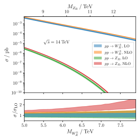
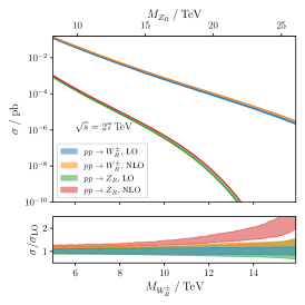
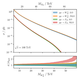
Figure 1: Production cross-sections for $W_{R}$ and $Z_{R}$ at LO and NLO for $\sqrt{s}=14,27$ and $100$ TeV. The lower part shows the $K$-factor, in which the shaded regions denote the scale- and pdf-uncertainties added in quadrature. Note that $M_{Z_{R}}$ is shown on the top $x$ axis and explains the kinematic suppression of $pp\to Z_{R}$ for large $M_{Z_{R}}$.

A few technical notes are useful:

• In case the chosen physical inputs lead to non-perturbative couplings, Madgraph may issue a WARNING: Failed to update dependent parameter. and results will probably be invalid. We recommend checking the ranges of chose physical inputs with the LRSMEVAL function described above, or with the equivalent Python code. The python code is shipped with a jupyter notebook in which its usage is explained. Apart from providing input parameters in the form of a dictionary, it also includes a “param_card reader” that automatically converts the parameters stored in a Madgraph param_card.dat to the internal syntax.

• For the full model files at NLO, or if neutrinos masses and Dirac couplings are not restricted to zero, update of card parameters in Madgraph hits a time constraint and the following warning is issued: WARNING: The model takes too long to load so we bypass the updating of dependent parameter. .... In this case should insert an "update dependent" command just after card edition, before event generation.

• The coupling orders of all interactions are just QED or QCD, with usual hierarchy QED=2, QCD=1.

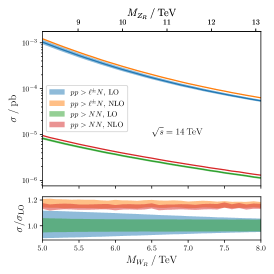
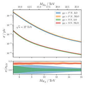
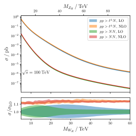
Figure 2: Inclusive production cross-sections for $pp\to\ell^{\pm}N$ ($\ell^{\pm}=e^{\pm},\mu^{\pm},\tau^{\pm}$, $N=N_{1},N_{2},N_{3}$) and $pp\to NN$ at LO and NLO for $\sqrt{s}=14,27,100\,\text{TeV}$. The lower part shows the $K$-factor in which the shaded regions denote the scale- and pdf-uncertainties added in quadrature.

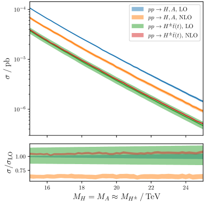
Figure 3: Production cross-sections for $H$, $A$ and $H^{\pm}$ (together with a (anti-)top quark) for $\sqrt{s}=100\,\text{TeV}$. The lower part shows the $K$-factor in which the shaded regions denote the pdf and scale uncertainties added in quadrature.

V Benchmarks

In this section we give an overview of a few example processes that can be consistently studied at NLO in QCD with the new model file. For all processes considered we use the following computational setup:

• We use the mlrsm-nu-loop version of the model file (5 dynamical flavours, charged lepton and light neutrino masses/yukawas have been set to zero).

• All parameters are fixed to their default values as shown in Table 4 unless otherwise indicated.

• We only compute the fixed-order cross sections without hadron shower at LO and NLO.

• We use MadGraph5_aMC_v3.5.3 [120] with LHAPDF 6.5.4 [121] with default settings.

• The pdfsets are NNPDF40_nlo_as_01190 [122] (lhaid=334100).

• For the factorization and renormalization scales we use the default dynamical scale scheme, e.g. for leading order processes dynamical scale scheme #4 ($\mu_{F}=\mu_{R}=\sqrt{\hat{s}}$); pdf and scale uncertainties are added in quadrature.

In order to estimate the impact of NLO QCD corrections, we define the $K$-factor as

$$K=\frac{\sigma\pm\delta\sigma}{\sigma_{\text{LO}}}\,,$$ (150)

in which $\delta\sigma$ denotes the uncertainty due to pdf uncertainties (estimated from the pdf replicas) and scale variation. The factorization scale $\mu_{F}$ and the renormalization scale $\mu_{R}$ are taken dynamical as $\mu_{F,R}=S_{F,R}\sqrt{\hat{s}}$, where $\hat{s}$ is the partonic center of mass energy and $S_{F,R}$ is a scale factor. The residual scale dependence is estimated by varying the scale factors $S_{F,R}$ independently on the interval $[\frac{1}{2},1,2]$ leading to 9 different values of the cross-section. As the central value one takes $S_{F}=S_{R}=1$, while the scale variation is quoted as the envelope of the largest negative/positive deviation. Generally, one can expect that NLO corrections lead to a decrease of this residual scale dependence due to an order-by-order absorption of the involved scale-dependent terms.

Let us begin by studying the Drell-Yan production cross sections of the new massive gauge bosons. In Figure 1 we show the $2\to 1$ cross-sections of $pp\to W_{R}^{\pm}$ and $pp\to Z_{R}$ for $\sqrt{s}=14,\>27$ and $100\>\mathrm{TeV}$ for a wide range of masses $M_{W_{R}^{\pm}}$ and $M_{Z_{R}}\approx 1.67M_{W_{R}^{\pm}}$ (cf. Eq.(26)). Note that the mass $M_{Z_{R}}$ is given in secondary $x$-axis on top. In the lower parts of the plots we show the LO and NLO $K$-factors in which the shaded regions denote the uncertainty due to pdf uncertainties and scale variation. The NLO corrections lead to an increase of the cross-section of order $\mathcal{O}(10-20\%)$ and lead to a reduction of the scale dependence from $\mathcal{O}(10-15\%)$ to $\mathcal{O}(2-5\%)$. For larger masses $M_{Z_{R}}$ close to the kinematic threshold, the $Z_{R}$ production cross-section strongly decreases while the size of the NLO corrections and also scale dependence strongly increase. The production cross section strongly increases with center of mass energy by three orders of magnitude between $\sqrt{s}=14$ TeV and $\sqrt{s}=100$ TeV.

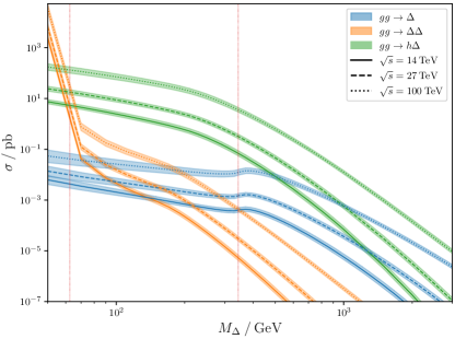
Figure 4: Production cross-sections for $gg\to\Delta$ (blue), $gg\to\Delta\Delta$ (orange) and $gg\to h\Delta$ (green) for $\sqrt{s}=14$, $27$, $100\,\text{TeV}$ (solid, dashed and dotted boundaries respectively). The shaded region denotes the pdf and scale uncertainty added in quadrature, while the vertical red lines denote the Higgs mass threshold ($M_{\Delta}=\frac{M_{h}}{2}$) and the top mass threshold ($M_{\Delta}=2M_{t}$).

In Figure 2 we show our results for the inclusive production cross sections $pp\to\ell^{\pm}N$ and $pp\to NN$, in which $\ell^{\pm}=e^{\pm}\,,\mu^{\pm}$ and $\tau^{\pm}$, while $N=N_{1}\,,N_{2}$ and $N_{3}$ (except for $pp\to NN$ at $\sqrt{s}=14$ TeV, since only $N_{1}$ and $N_{2}$ are kinematically accessible). Since the $\ell^{\pm}N$ ($NN$) production is dominantly mediated via the Drell-Yan process $pp\to W_{R}^{\pm}(Z_{R})\to\ell^{\pm}N(NN)$, we observe a very similar impact of the NLO corrections as for the $pp\to W_{R}^{\pm},Z_{R}$ production cross-sections. With our choice of the heavy neutrino masses (cf. Table 4), both cross sections are dominated by having $N_{1}$ in the final state.

The Drell-Yan production cross-sections for heavy (pseudo-) scalars $A$ and $H$ as well as the heavy charged scalar $H^{\pm}$ (with an additional (anti-) top quark in the final state) proceeds mostly via initial state $b$-quarks and a gluon, while gluon initiated processes give a 2-3 order of magnitude smaller contribution. In Figure 3 we show our results for the $pp\to H^{\pm}\bar{t}(t)$ production cross-sections for $\sqrt{s}=100$ TeV. The masses $M_{H}$ and $M_{A}$ are set equal, while the mass $M_{H^{\pm}}$ is degenerate with $M_{A}$ up to order $\epsilon^{2}$ corrections.

Firstly, we notice that for $pp\to A,H$ the NLO corrections lead to a significant decrease of the cross section by $30-40\%$, due to reduced high scale top Yukawa, while the scale dependence slightly increases. The NLO corrections $pp\to H^{\pm}\bar{t}(t)$ lead to a mild increase of the cross section and a significant reduction of the scale variation from $\mathcal{O}(15-20\%)$ to $\mathcal{O}(1-2\%)$.

Next, we consider several production mechanisms of the neutral scalar $\Delta$. Since $\Delta$ mostly comes from the real part of the neutral component of the right-handed triplet $\Delta_{R}$, it couples to quarks only through mixing with with the SM-like scalar $h$. Therefore, its largest quark coupling is to the top quark, making different type of gluon fusion processes the dominant production mechanisms. Since gluon fusion is a loop-induced process, we can only consider the leading order cross-sections within the scope of Madgraph and this model file. In particular, we consider single- and pair production via gluon fusion $gg\to\Delta,\Delta\Delta$ as well as “Higgs-$\Delta$-strahlung” $gg\to h\Delta$ which proceeds both via $gg\to h\to h\Delta$, as well as $gg\to\Delta\to h\Delta$ in addition to sub-leading box-topologies. In Figure 4 we show our results for these production mechanisms for $m_{\Delta}\in(50,3000)$ GeV for $\sqrt{s}=14\,,27$ and $100$ TeV. Firstly, we notice that for $M_{\Delta}\simeq 2m_{t}$ (denoted by the right vertical red line) the $gg\to\Delta$ cross section increases due to threshold effects in the corresponding “top-triangle”, before it drops off for larger masses. Next, for $M_{\Delta}\lesssim M_{h}/2$ (denoted by the left vertical red line), the $gg\to\Delta\Delta$ production cross section becomes large due to an on-shell intermediate Higgs in $gg\to h\to\Delta\Delta$. Above threshold, the cross-section strongly decreases and becomes somewhat subdominant. Lastly, the process $gg\to h\Delta$ is the dominant production mechanism for a wide range of masses $M_{\Delta}\in(M_{h}/2,\sim 500)$ GeV, competing with $gg\to\Delta$ for larger masses.

In addition to the aforementioned “benchmark processes”, we also checked several SM processes with the LRSM model file, such as $pp\to t\bar{t}$ and $gg\to h\to t\bar{t}$ production cross-sections, finding perfect agreement with the built-in MadGraph models. Finally, in Table 5 we summarize our results for the choice of parameters given in Table 4 as a representative benchmark point. This phenomenological study is by no means complete and rather serves as a proof of concept. With this model file, fully consistent collider studies (cross-section calculation and event generation) are possible with NLO QCD corrections as well as the study of loop-induced processes at LO. The NLO corrections generally lead to a significant decrease of the scale dependence and therefore to a significant reduction of signal modelling uncertainties for collider studies.

$\begin{array}[]{|c|c|c|c|c|}\hline\cr\hbox{\multirowsetup Process}&\sigma_{\text{LO}}&\sigma_{\text{NLO}}&\hbox{\multirowsetup$K$}&\sqrt{s}\\[-4.2194pt] &[\mathrm{fb}]&[\mathrm{fb}]&&[\mathrm{TeV}]\\[3.01389pt] \hline\cr\hline\cr&0.636_{-13\%}^{+16\%}&0.806_{-5.4\%}^{+4.4\%}&1.27&14\\ pp\to W_{R}^{\pm}&38.21_{-9.4\%}^{+11\%}&46.0_{-3.2\%}^{+2.6\%}&1.20&27\\ &1572_{-3.0\%}^{+3.2\%}&1791_{-1.2\%}^{+1.2\%}&1.14&100\\ \hline\cr&7.0_{-20\%}^{+26\%}\times\!10^{-5}&10.6_{-10\%}^{+10\%}\times\!10^{-5}&1.52&14\\ pp\to Z_{R}&0.16_{-12\%}^{+14\%}&0.20_{-4.4\%}^{+3.5\%}&1.25&27\\ &59.9_{-5.2\%}^{+5.7\%}&68.6_{-1.6\%}^{+1.5\%}&1.15&100\\ \hline\cr&0.29_{-8\%}^{+10\%}&0.34_{-3.0\%}^{+2.3\%}&1.17&14\\ pp\to\ell^{\pm}N&2.79_{-9\%}^{+11\%}&3.22_{-2.7\%}^{+1.8\%}&1.15&27\\ &271.0_{-2.9\%}^{+3.0\%}&303.3_{-1.1\%}^{+1.2\%}&1.12&100\\ \hline\cr&3.72_{-4.5\%}^{+5.0\%}\times\!10^{-3}&4.24_{-1.8\%}^{+1.7\%}\times\!10^{-3}&1.14&14\\ pp\to NN&6.7_{-7\%}^{+8\%}\times\!10^{-2}&7.75_{-2.4\%}^{+1.8\%}\times\!10^{-2}&1.15&27\\ &6.8_{-5.1\%}^{+5.6\%}&7.59_{-1.3\%}^{+1.1\%}&1.11&100\\ \hline\cr\hbox{\multirowsetup$pp\to H$}&8.1_{-16\%}^{+21\%}\times\!10^{-12}&7.2_{-5.2\%}^{+2.2\%}\times\!10^{-12}&0.89&27\\ &1.11_{-3.2\%}^{+2.9\%}\times\!10^{-2}&7.0_{-6.0\%}^{+5.7\%}\times\!10^{-3}&0.63&100\\ \hline\cr\hbox{\multirowsetup$pp\to A$}&8.0_{-16\%}^{+21\%}\times\!10^{-12}&7.1_{-5.2\%}^{+2.2\%}\times\!10^{-12}&0.89&27\\ &1.10_{-3.2\%}^{+2.9\%}\times\!10^{-2}&7.0_{-6.0\%}^{+5.7\%}10^{-3}&0.63&100\\ \hline\cr\hbox{\multirowsetup$pp\to H^{\pm}\bar{t}(t)$}&8.0_{-25\%}^{+36\%}\times\!10^{-13}&1.0_{-10\%}^{+7\%}\times\!10^{-12}&1.35&27\\ &3.8_{-14\%}^{+18\%}\times\!10^{-3}&4.0_{-2.3\%}^{+1.2\%}\times\!10^{-3}&1.06&100\\ \hline\cr&0.19_{-20\%}^{+26\%}&--&--&14\\ gg\to\Delta&0.84_{-17\%}^{+21\%}&--&--&27\\ &8.6_{-20\%}^{+25\%}&--&--&100\\ \hline\cr&2.7_{-22\%}^{+31\%}\times\!10^{-4}&--&--&14\\ gg\to\Delta\Delta&2.0_{-19\%}^{+26\%}\times\!10^{-3}&--&--&27\\ &3.8_{-14\%}^{+17\%}\times\!10^{-2}&--&--&100\\ \hline\cr&8.5_{-21\%}^{+29\%}&--&--&14\\ gg\to\Delta h&46._{-18\%}^{+23\%}&--&--&27\\ &620._{-16\%}^{+20\%}&--&--&100\\ \hline\cr\end{array}$

Table 5: Example cross sections for the set of input parameters given in Table 4. The (super)sub-scripts denote the (upper)lower envelope due to pdf and scale uncertainties. We also quote the central $K$-factor.

VI Summary and outlook

The main purpose of this work was to provide an implementation of the LRSM, which is as complete as possible and can be used for a variety of collider and other phenomenological studies. The collider frontier in the near future will mostly be focused on the HL-LHC, but in the less near future we may expect to see lepton colliders FCC-ee, ILC, CLIC or muon colliders, and finally high energetic scatterings of protons in FCC-eh or FCC-hh at few tens of TeV (30 or 100 TeV). With the present model file, the NLO QCD corrections can be reliably calculated for any process within the LRSM, properly including the mixings of scalars, gauge bosons and fermions in different gauges, too. Not all the parts of the model are necessarily needed for simulations, even very precise ones, therefore we provide a number of restricted versions, which may be faster and easier to use.

Perhaps the most significant analytical developments in this work are the explicit calculation of heavy-light neutrino mixing and the solution of the scalars spectrum.

For neutrinos, the Majorana-Dirac connection was found some time ago [63], but with the help of the Cayley-Hamilton theorem, we managed to come up with a closed form solution for a general complex matrix in terms of its invariants. This relation may become very useful to clarify the flavor relations in the leptonic sector, e.g. how the Dirac induced transitions (in eEDMs, $0\nu 2\beta$, collider of $N_{1}\to\nu\gamma$) are related to the flavor structure of $V_{R}$ and the $m_{N}$ mass spectrum. The explicit result allows for a direct insight by taking certain expansions (small angles or masses) or correction to limits, like type II (sub)dominance.

In the scalar sector, the mass spectrum was derived for the first time without extra assumptions of small mixing angles, thus performing an exact diagonalization. The only phenomenologically required assumption was that the Higgs field $h$ has a limited admixture with heavy scalars. Remarkably, we were able to derive exact expressions for the model couplings in terms of scalar masses and mixings, which can cover both the standard regime of heavy scalars as well as the regime of light $\Delta$. The latter case is relevant for the Majorana-Higgs program, but the implemented mixings cover the regimes of quasi-degeneracy, too. Criteria for perturbativity of the chosen inputs were explicitly identified, and provided as an implemented routine.

The model capabilities were demonstrated on a number of benchmarks concerning the single production of heavy resonances, $pp\to W_{R},Z_{R}$, various scalars $pp\to\Delta,H^{\pm}$ and production of heavy neutrinos $pp\to\ell N$, $pp\to NN$, calculated at the NLO level in QCD.

A foreseeable improvement might be the inclusion of electroweak corrections. These could be used to automatize the computation of various electroweak precision observables and calculate one loop processes, like radiative production and decays at one loop. Such an analysis may not be impossible but it would require going beyond the current state of the art, given the complexity of the model. We shall leave it for a future study. The payoff might be having precise and automatized control over rare processes that might be possible to explore at future colliders.

Appendix A Square root(s) of a $3\times 3$ matrix

We calculate the closed form analytic expression for the 8 square roots of a general complex $3\times 3$ matrix using the Cayley-Hamilton theorem. For some of the previous work, see [123, 124, 125]. We start by writing the invariants of $A$ and $\sqrt{A}$

$$T =\text{tr }A\,, T_{1/2} =\text{tr }\sqrt{A}\,,$$ (151)

$$T_{2} =\text{tr }A.A\,, T_{2,1/2} =\text{tr }\sqrt{A}.\sqrt{A}=T\,,$$ (152)

$$\Delta =\det A\,, \Delta_{1/2} =\det\sqrt{A}=\sqrt{\Delta}\,,$$ (153)

where the trace of the square of $\sqrt{A}$ and its determinant are trivially related to the invariants of $A$. Cayley-Hamilton theorem states that matrices themselves are solutions to their characteristic polynomial equations, which can be written in terms of invariants

$$A^{3}-TA^{2}+\tilde{T}A-\Delta\,\mathbb{1} =0\,, \ \tilde{T}=\frac{1}{2}\left(T^{2}-T_{2}\right).$$ (154)

The same holds for the square root that obeys a polynomial with its own invariants (two of which are directly related to the invariants of $A$)

$$\left(\sqrt{A}\right)^{3}-T_{1/2}\left(\sqrt{A}\right)^{2}+\tilde{T}_{1/2}\sqrt{A}-\sqrt{\Delta}\,\mathbb{1} =0\,,$$ (155)

$$\tilde{T}_{1/2}=\frac{1}{2}\left(T_{1/2}^{2}-T\right),$$ (156)

$$A\sqrt{A}-T_{1/2}A+\tilde{T}_{1/2}\sqrt{A}-\sqrt{\Delta}\,\mathbb{1} =0\,.$$ (157)

We can get to a linear equation for $\sqrt{A}$ by multiplying (157) with $\sqrt{A}$

$$A^{2}-T_{1/2}A\sqrt{A}+\tilde{T}_{1/2}A-\sqrt{\Delta}\sqrt{A} =0\,,$$ (158)

$$A^{2}-T_{1/2}\left(T_{1/2}A-\tilde{T}_{1/2}\sqrt{A}+\sqrt{\Delta}\,\mathbb{1}\right)+\quad$$

$${}+\tilde{T}_{1/2}A-\sqrt{\Delta}\sqrt{A} =0\,,$$ (159)

which finally gives

$$\sqrt{A} =\pm\frac{A^{2}+\left(\tilde{T}_{1/2}-T_{1/2}^{2}\right)A-\sqrt{\Delta}\,T_{1/2}\,\mathbb{1}}{\sqrt{\Delta}-T_{1/2}\tilde{T}_{1/2}}\,.$$ (160)

This is already a striking result, where we know the off-diagonal flavor structure of the root directly from a power expansion of $A$, terminating at the second order (as expected for $3\times 3$ matrices from the Cayley-Hamilton theorem).

All the non-linearity is hidden in the equation for the remaining invariant $T_{1/2}$, which we get by taking the trace of (A) and using (156), such that

$$T_{1/2}^{4}-2T\,T_{1/2}^{2}-8\sqrt{\Delta}\,T_{1/2}+2T_{2}-T^{2}=0\,.$$ (161)

This is a depressed quartic with four possible solutions

$$T_{1/2} =\frac{\pm\eta_{s}+s\,\chi}{2\sqrt{6\xi}}\,, s =\pm\,,$$ (162)

which in turn give four corresponding $\tilde{T}_{1/2}$ via (156). The shorthands $\xi$, $\chi$, $\eta_{\pm}$, are only functions of the invariants of $A$ and are found from these expressions:

$$\xi^{3} =-32\left(5T^{3}-9TT_{2}-54\Delta\right)+96\sqrt{3\left(T^{2}-2T_{2}\right)\left(T^{2}-T_{2}\right)^{2}+12T\left(9T_{2}-5T^{2}\right)\Delta+324\Delta^{2}}\,,$$ (163)

$$\chi^{2} =-16\,\sqrt[3]{2}\,T^{2}+48\,\sqrt[3]{2}\,T_{2}+8T\xi+\sqrt[3]{4}\,\xi^{2}\,,$$ (164)

$$\eta_{\pm}^{2} =16\,\sqrt[3]{2}\left(T^{2}-3T_{2}\right)+\xi\left(16T-\sqrt[3]{4}\,\xi\pm 96\sqrt{6}\,\chi^{-1}\sqrt{\Delta\xi}\right),$$ (165)

where one assumes positive roots only. Together with the overall sign in (160), we get the total of 8 matrix roots.

With an explicit expression for $\sqrt{A}$, it is also easy to get the inverse root, by multiplying (157) with $A^{-1/2}$,

$$A-T_{1/2}\sqrt{A}+\tilde{T}_{1/2}\,\mathbb{1}-\sqrt{\Delta}\,A^{-1/2}=0\,,$$ (166)

so that the inverse root is found as

$$\left(\sqrt{A}\right)^{-1}=\frac{1}{\sqrt{\Delta}}\left(A-T_{1/2}\sqrt{A}+\tilde{T}_{1/2}\,\mathbb{1}\right).$$ (167)

Again, there are eight possible branches and also the form of this solution is a matrix power expansion up to $A^{2}$.