X. Crean^1$\star$, J. Giansiracusa^2$\dagger$ and B. Lucini^1$\ddagger$

Abstract

In $4$-dimensional pure compact $U(1)$ lattice gauge theory, we analyse topological aspects of the dynamics of monopoles across the deconfinement phase transition. We do this using tools from Topological Data Analysis (TDA). We demonstrate that observables constructed from the zeroth and first homology groups of monopole current networks may be used to quantitatively and robustly locate the critical inverse coupling $\beta_{c}$ through finite-size scaling. Our method provides a mathematically robust framework for the characterisation of topological invariants related to monopole currents, putting on firmer ground earlier investigations. Moreover, our approach can be generalised to the study of Abelian monopoles in non-Abelian gauge theories.

 

Contents

1. 1 Introduction
2. 2 $U(1)$ Lattice Gauge Theory
   1. 2.1 The Model
   2. 2.2 Topology of Monopole Currents and Phase Structure of the Model
   3. 2.3 Estimating the Critical Inverse Coupling $\beta_{c}$
3. 3 Topological Data Analysis
   1. 4 Conclusion and Discussion
      1. A Dirac Sheets
      2. B Methods
         1. B.1 Histogram Reweighting
         2. B.2 Bootstrap Error Estimation
      3. C Background on Homology
         1. C.1 Chain Complex
         2. C.2 Homology of a Graph
      4. D Finite-size Scaling Analysis: Further Details

 

1 Introduction

Providing a consistent explanation of confinement in non-abelian lattice gauge theory has been a sought-after objective for more than 50 years. Prominent avenues of research involve the analysis of two topological objects, respectively centre vortices and monopoles. Ever since Polyakov showed in [1] that, in the $3$-dimensional compact QED vacuum, a monopole gas provides a consistent abelian linear confinement mechanism by screening electric probes, there has been significant interest in the abelian monopole picture of confinement. Mandelstam [2] and ’t Hooft [3] suggested that a dual superconductor model of confinement may be formulated such that a dual Meissner effect expels electric flux lines from the bulk except for collimated tubes between charges. As suggested by Wilson in [4], in the case of $4$-dimensional pure compact QED, this manifests as a bulk phase transition between a confining phase and a Coulomb phase. At strong coupling, Cooper pairs of magnetic monopoles condense and thus induce a dual Meissner effect such that electric charges are confined [5, 6]. DeGrand and Toussaint’s pioneering work in [7] outlined a way to measure monopoles in lattice simulations and demonstrated the existence of a phase transition involving monopoles with critical inverse coupling $\beta_{c}\approx 1.01$. Subsequent work (e.g., Refs. [8, 9]) highlighted the role of monopoles in the phase transition. Further, by considering the Dirac sheets, Kerler et al. confirmed in [10] that the transition may be characterised as a percolation-type transition where, in the confining phase, monopole currents fill the volume in all four spacetime directions. An order parameter based on monopole condensation was formulated and studied in [11], while a more recent investigation of the phases of the model and of the role that monopoles play in its dynamics is provided in [12]. A different approach to the transition based on observables inspired by the XY model is provided in [13].

Following the first numerical explorations of the model [14, 15, 16, 17, 18], even though the dynamics of the system became well understood and the existence of a phase transition unambiguously demonstrated, the order of this phase transition was debated for a long time [19, 20, 21, 22, 23, 24, 25, 26, 27, 28, 29]. Simulations that involve small lattice sizes obscure the double-peak structure of action histograms and thus make it difficult to identify the order of the transition. Whereas, for larger lattice sizes, there exists a limitation in Monte Carlo simulations known as critical slowing down caused by severe meta-stabilities in the critical region of the transition due to the condensation of monopoles. Monopole currents self-organise in large percolating networks that wrap around a lattice with periodic boundary conditions, forming potential barriers between states of the system, and these cost a large amount of energy to break apart. In the critical region, as the lattice size increases, the probability of tunnelling between confining and Coulomb phases becomes exponentially suppressed, which means that Markov chain simulations can take a very long time to sample the configuration space sufficiently to precisely estimate $\beta_{c}$. Only relatively recently, with the emergence of high-performance computing and specialised numerical methods, has this been confirmed as a weak first order transition [30, 31].

When one considers percolating current networks and their unwinding mechanism, framed in this way, the problem of monopole condensation has a topological nature. On a finite-size, periodically closed lattice, monopole current lines necessarily form closed loops, which can either be global (wrapping around a direction on the hyper-torus) or local (non-wrapping), and can be connected in large, self-intersecting networks or be separated into distinct, small networks. This poses a question about whether the study of topological invariants associated to the monopole current networks across the phase boundary may yield useful quantitative information.

More generally, topological phase structure has been studied in a variety of lattice theories. In the generalised Ising model, Blanchard et al. in [32] found a sharp transition in the Euler characteristic and Betti numbers of a cubical complex constructed by considering clusters of aligned spins. Recently, Topological Data Analysis (TDA), a field combining algebraic topology and data science, has materialised as a range of tools for analysing topological structures in datasets in a highly interpretable way. This has been used to probe various physical models and associated critical phenomena [33, 34, 35, 36, 37, 38, 39, 40, 41, 42, 43, 44, 45, 46] (a useful survey is [47]) including the confinement-deconfinement phase transition in non-abelian lattice gauge theory (and related effective models) [48, 49, 50, 51, 52, 53]. Typically, topological structure in a given lattice configuration is analysed by computing the Betti numbers of a purpose-built hierarchy of cubical complexes (called a filtration) in a process known as persistent homology. In the case of $4$-dimensional $SU(2)$ lattice gauge theory, persistent homology allowed Sale et al. in [51] to extract the critical exponents of the continuous deconfinement transition by computing the homology associated to structures built from $2$-dimensional vortex surfaces.

In a similar vein, we approach the well-studied discontinuous deconfinement transition in $4$-dimensional compact $U(1)$ lattice gauge theory but, since monopole currents are oriented $1$-dimensional strings, we can use a simpler, readily computable application of TDA. Our novel contribution is to demonstrate that observables constructed explicitly from the homology of monopole current networks, when considered as directed graphs, allow the critical inverse coupling $\beta_{c}$ to be estimated robustly. Compared to the work of Kerler et al. [10], where one must compute Dirac sheets of minimal area via annealing, our methodology is a computationally more efficient way to systematically analyse the topological phase structure of a lattice configuration. Further, our work may be seen as a preliminary step in the application of computational topology tools to analyse the abelian confinement mechanisms in more general Yang-Mills lattice gauge theories.

The paper is structured as follows. In Section 2, we provide a background on $4$-dimensional pure compact $U(1)$ lattice gauge theory; we then introduce the DeGrand-Toussaint prescription of Dirac monopoles and the deconfinement phase transition formulated in terms of monopole currents. In Section 3, we explain how topological observables constructed from monopole current networks may be used to quantitatively analyse the phase structure of a lattice configuration and present our results for estimating the critical inverse coupling $\beta_{c}$ of the phase transition. In Section 4, we conclude and discuss potential future work. In the appendices, we provide additional content including a background on homology.

2 $U(1)$ Lattice Gauge Theory

2.1 The Model

We consider pure 4-dimensional lattice gauge theory with gauge group $U(1)$. To establish notation, our lattice is $\Lambda=\{1,\ldots,L\}^{4}$ with periodic boundary conditions, so it is a discretisation of the 4-torus $T^{4}=S^{1}\times S^{1}\times S^{1}\times S^{1}$. If $\mu=0,\ldots,3$ indexes directions, then links are indexed by pairs $(x\in\Lambda,\mu)$ connecting sites $x$ and $x+\hat{\mu}$, and plaquettes are indexed by a lattice site $x\in\Lambda$ and a pair of directions $\mu\nu$. The gauge field $U$ assigns an element $U_{\mu}(x)\in U(1)$ to each link. We represent elements of $U(1)$ by angular parameters $\theta\in(-\pi,\pi]$, so $U_{\mu}(x)=e^{i\theta_{\mu}(x)}$.

The Wilson loop around the plaquette $(x,\mu\nu)$ is

$$U_{\mu\nu}(x)\equiv U_{\mu}(x)U_{\nu}(x+\hat{\mu})U^{*}_{\mu}(x+\hat{\nu})U^{*}_{\nu}(x)$$ (1)

where $U^{*}_{\mu}(x)$ is the complex conjugate of $U_{\mu}(x)$. In terms of the angular variables, we have $U_{\mu\nu}(x)=e^{i\theta_{\mu\nu}(x)}$ with $\theta_{\mu\nu}(x)=\theta_{\mu}(x)+\theta_{\nu}(x+\hat{\mu})-\theta_{\mu}(x+\hat{\nu})-\theta_{\nu}(x)$. Given a gauge field configuration $U$, one then defines the Wilson action in terms of the angular parameters as

$$S=\beta\sum_{x,\mu<\nu}\left(1-\cos[\theta_{\mu\nu}(x)]\right)$$ (2)

where $\beta=\frac{1}{g^{2}}$ with $g$ the gauge coupling such that in the classical continuum limit, where the lattice spacing $a\to 0$, we have the Yang-Mills action [4].

The partition function is a path integral of the form

$$Z=\int\mathcal{D}\theta e^{-S(\theta)}$$ (3)

with the path integral measure given by a product of Haar measures,

$$\mathcal{D}\theta=\prod_{x,\mu}d\theta_{\mu}(x).$$ (4)

The vacuum expectation value of an observable $O$ is defined as

$$\langle O\rangle=\frac{1}{Z}\int\mathcal{D}\theta O(\theta)e^{-S(\theta)}.$$ (5)

In practice, we generate $N$ samples via Monte Carlo simulation and compute the sample observables $\{O_{i}\}_{i=0}^{N-1}$. We may then estimate $\langle O\rangle$ by the mean of the sample observables:

$$\langle O\rangle\approx\frac{1}{N}\sum_{i=0}^{N-1}O_{i}.$$ (6)

2.2 Topology of Monopole Currents and Phase Structure of the Model

The phase transition in $4d$ compact $U(1)$ is mediated by the condensation of monopoles, such that, in the strong coupling regime $\beta<\beta_{c}$, we have an electrically confining phase and, in the weak coupling regime $\beta>\beta_{c}$, we have a free Maxwell theory. Note that, in analogy with inverse temperature $\beta\equiv\frac{1}{k_{B}T}$ in statistical physics, we shall refer to the low-$\beta$ phase as hot and the high-$\beta$ phase as cold.

In a single time slice, gauge invariant monopoles are the endpoints of $1$-dimensional non-gauge invariant singularities called Dirac strings (that can be thought of as infinitely thin solenoids). Given a lattice gauge field configuration, we can measure Dirac strings by noting that they carry units of $2\pi$ flux. Since plaquette variables represent the electromagnetic field strength tensor, i.e., $\theta_{\mu\nu}(x)=a^{2}F_{\mu\nu}(x)+O(a^{3})$ with lattice spacing $a$, they measure the magnetic flux of the corresponding $1\times 1$ square area of the plaquette. Since link variables $\theta_{\mu}(x)$ take values in the interval $(-\pi,\pi]$, the plaquette variables $\theta_{\mu\nu}(x)$ are valued in $(-4\pi,4\pi]$; the physical plaquette angle is defined as

$$\bar{\theta}_{\mu\nu}(x)\equiv\theta_{\mu\nu}(x)-2\pi\,n_{\mu\nu}(x)\quad\in[-\pi,\pi],$$ (7)

where $n_{\mu\nu}(x)\in\{0,\pm 1,\pm 2\}$ is interpreted as the number of Dirac strings through the plaquette [7]. The gauge invariant monopole number in any given $3$-cube may be computed by counting the net number of Dirac strings entering/exiting the volume. Thus, for each lattice site $x\in\Lambda$, we have four monopole numbers given by the relation

$$M_{\rho}(x) =\frac{1}{4\pi}\varepsilon_{\rho\sigma\mu\nu}[\bar{\theta}_{\mu\nu}(x+\hat{\sigma})-\bar{\theta}_{\mu\nu}(x)]$$

$$=\varepsilon_{\rho\sigma\mu\nu}[n_{\mu\nu}(x+\hat{\sigma})-n_{\mu\nu}(x)]$$ (8)

(c.f. $3d$ continuum Maxwell equation $M(\vec{x})=\frac{1}{4\pi}\partial_{i}B_{i}(\vec{x})$).

We may naturally define the dual lattice $\Lambda^{*}$ where $4$-cubes are dual to vertices, $3$-cubes dual to links, $2$-cubes dual to $2$-cubes etc. On $\Lambda^{*}$, given that links are dual to $3$-cubes, monopole worldlines are represented by $4$-currents $j_{\rho}(x)=M_{\rho}(x+\hat{\rho})$ that are defined on links (Figure 1).

Figure 1: Given $x+\hat{\rho}\in\Lambda$, to visualise a dual lattice $4$-current $j_{\rho}(x)=+1$ piercing a lattice $3$-cube $M_{\rho}(x+\hat{\rho})$, we consider a three-dimensional analogue where a lattice $2$-cube (grey) is pierced by a dual lattice $1$-cube (red).

Given an appropriate orientation, we have that

1. $j_{\rho}(x)=0\implies\nexists$ current line on link at $x$

2. $j_{\rho}(x)=\pm 1\implies\exists$ one current line on link at $x$

3. $j_{\rho}(x)=\pm 2\implies\exists$ two current lines on link at $x$

which must obey the conservation of current

$$\sum_{\rho}[j_{\rho}(x)-j_{\rho}(x-\hat{\rho})]=0$$ (9)

(c.f. $\partial_{\rho}j_{\rho}=0$). This implies that the current lines must form a union of closed loops. Since we have periodic and untwisted boundary conditions, the charge of periodically closed current loops must be zero, i.e., for a given loop that wraps around a given direction on $T^{4}$, there must also be an oppositely oriented partner loop.

Defining a network as a connected set of current lines and a Dirac sheet as the worldsheet of a Dirac string such that the boundary of a Dirac sheet is a current loop (see Appendix A), Kerler et al. [10] characterised the phase structure of the system as follows:

1. Configurations sampled from the hot phase ($\beta<\beta_{c}$) contain (with high probability) a Dirac sheet with boundary of non-trivial winding number around the torus in each of the four directions, and hence a percolating current network in each direction.

2. For configurations sampled from the cold phase ($\beta>\beta_{c}$), all Dirac sheets have a boundary that is homotopically trivial (with high probability), and hence there does not exist a percolating current network. Note that, subject to conditions, non-trivial Dirac sheets without boundary may form, giving rise to meta-stable states [19].

In the hot phase, whilst there is a large, entangled, percolating current network, there may also exist small networks that do not form part of the largest network, since it is energetically favourable to produce a monopole-antimonopole pair. In the cold phase, we only have non-percolating current loops. In Figure 2, we have a two-dimensional schematic of a configuration in the hot/cold phase.

(a)

(b)

Figure 2: In this schematic, we have a two-dimensional analogue of an example configuration where the dashed grey lines represent the periodic boundary of $T^{2}=S^{1}\times S^{1}$ and the black arrows represent monopole current networks. In Figure 2, the configuration is in the hot phase and so has a percolating current network as well as isolated, small current networks. In Figure 2, we have only small current networks.

2.3 Estimating the Critical Inverse Coupling $\beta_{c}$

There does not exist a way to compute the critical inverse coupling $\beta_{c}$ of the phase transition analytically. However, on finite-size lattices, one may compute the psuedo-critical coupling $\beta_{c}(L)$ via several different numerical methods. In the infinite volume limit $L\to\infty$, these psuedo-critical values converge to $\beta_{c}\approx 1.01$.

The phase transition in compact $U(1)$ has severe meta-stabilities at criticality which make generating configurations using Monte Carlo simulation a computationally expensive exercise. Simulations may become stuck in local minima of the action which take a very long time to tunnel out of. Specialised numerical methods have been developed to overcome these issues and have been able to estimate $\beta_{c}$ to a high degree of accuracy [54, 55].

The standard observable one uses to estimate $\beta_{c}$ is the average plaquette action

$$E=\frac{1}{6V}\sum_{x,\mu<\nu}\cos[\theta_{\mu\nu}(x)]$$ (10)

where volume $V=L^{4}$. Typically, one computes cumulants of $E$, such as the specific heat at constant volume

$$C_{V}(\beta)=6\beta^{2}V(\langle E^{2}\rangle-\langle E\rangle^{2}),$$ (11)

at many values of $\beta$, and then locates the pseudo-critical value $\beta_{c}(L)$ at which $C_{V}$ is maximal. The estimation of the location of the peak uses histogram reweighting, which is a technique for estimating the value of an observable at many interpolating $\beta$ values; for a review of histogram reweighting, see Appendix B.1.

Using these psuedo-critical $\beta_{c}(L)$, we may estimate the infinite volume limit of the critical coupling $\beta_{c}$ via a finite-size scaling analysis given the asymptotic relation

$$\beta_{c}(L)=\beta_{c}+\sum_{k=1}^{\infty}B_{k}L^{-4k},$$ (12)

where the sum may be truncated by parameter $k_{max}<\infty$. Further, we estimate the standard error via the bootstrapping method; for a review, see Appendix B.2.

Since this phase transition is weak first order (WFO), finite-size effects will obscure the double peak structure of action histograms for smaller lattice sizes. This is because, for a WFO transition, the critical correlation length $\xi_{c}$ is typically very large and, for small lattice volumes $L^{4}$, with $L$ the measure of one of the four equal edges of the lattice, we may have $L\leq\xi_{c}$. In this region, relative to the lattice, $\xi_{c}$ is effectively infinite and the transition behaves as if it were second order. To mitigate these pretransitional effects, we only take lattice sizes $L\geq 6$, which have been shown in the literature to present a double peak structure.

The goal of our analysis is to construct robust observables using topological data analysis of monopoles to estimate $\beta_{c}(L)$ for a suitable choice of finite lattice sizes, i.e.,
$L\in\{6,7,8,9,10,11,12\}$, in order to perform a finite-size scaling analysis to estimate $\beta_{c}$ in the infinite volume limit $L\to\infty$.

We generate $N=200$ lattice configurations using a Monte Carlo (MC) importance sampling method: each update consists of one heatbath update, consisting of an approximate heatbath step corrected by a Metropolis step [56], and five over-relax updates. Computing estimates of $\beta_{c}$, with low-statistics using this algorithm, of comparable accuracy and precision to literature reference values (see Table 1) would be very computationally expensive and is not our objective. Instead, we take a computationally feasible number of MC updates for each respective lattice size, i.e., $\geq 8.4\times 10^{6}$, and compute the $\beta_{c}$ given by the average plaquette observable $E$ which we expect to be close to the reference values but with a small systematic bias that can be quantified by comparing with the literature. We will then use the observable $E$ as a benchmark for our new topological observables, i.e., if a topological observable returns an estimate of $\beta_{c}$ statistically consistent with the fiducial value estimated via $E$, we claim that the topological observable acts as a phase indicator for the phase transition.

$L$	$\beta_{c}(L)$
6	1.001794(64)
8	1.00744(2)
10	1.00939(2)
12	1.010245(1)

Table 1: Reference $\beta_{c}(L)$ values, i.e., locations of the specific heat $C_{V}(\beta)$ maxima as a function of lattice size [54, 55].

3 Topological Data Analysis

As described in Section 2.2, a configuration in the confining phase contains a percolating monopole current network, whilst a configuration in the Coulomb phase does not. We construct simple topological observables from monopole current networks to estimate the critical inverse coupling $\beta_{c}$ via a finite-size scaling analysis. For a brief review on the homology of graphs, see Appendix C.

In a given lattice gauge field configuration, we may naturally endow the disjoint union of monopole current networks with the structure of a (possibly disconnected) directed graph. This is achieved by associating dual lattice links with $j_{\rho}(x)=\pm 1,\pm 2$ to directed graph edges such that an edge receives the orientation corresponding to the orientation of $j_{\rho}(x)$. Then, for each edge, we include its boundary vertices to complete the graph. Thus, we have an edge set $E$ consisting of directed current lines and vertex set $V$ consisting of their boundary vertices. We denote this monopole current graph by $X_{j}=(V,E)$.

By Equation (9), current networks are necessarily unions of closed loops. Note that these current loops may intersect. We compute the Betti numbers $b_{0}(X_{j})=\dim H_{0}(X_{j})$, the number of connected components of $X_{j}$, and $b_{1}(X_{j})=\dim H_{1}(X_{j})$, the number of loops of $X_{j}$. We use the coefficient field $\mathbb{Z}_{2}$ but, since this is a $1$-dimensional complex, the resulting Betti numbers are independent of the coefficient field.

In the cold phase ($\beta>\beta_{c}$), the currents typically form a disjoint collection of small loops, so $b_{1}\approx b_{0}$. In the hot phase, one typically sees a large percolating network consisting of many intersecting loops together with a few isolated small networks, and so $b_{1}>b_{0}$.

To construct more useful observables from $b_{0}$ and $b_{1}$ that can be directly compared across various lattice sizes, we normalise by the number of links, i.e., we compute the density of distinct networks $\rho_{b_{0}}$ and density of loops $\rho_{b_{1}}$.

As seen in Figure 3, the density $\rho_{b_{0}}$ reveals the signature of the phase transition. In the hot phase, the probability that small networks form alongside the large percolating network is non-zero; therefore, we have a small but non-zero number of connected components. As the temperature approaches the critical value, $\rho_{b_{0}}$ reaches a maximum value as the large percolating network is broken into smaller networks. As the temperature decreases, in the cold phase, the cost in action of generating a monopole current loop is expensive, hence the number of networks decreases. For all lattice sizes $L=6,...,12$, we find that the reweighted variance curves for $\rho_{b_{0}}$ peak at the critical point allowing us to extract the pseudo-critical $\beta_{c}(L)$ values.

As seen in Figure 4(a), we find that the observable $\rho_{b_{1}}$ acts as a phase indicator since the number of loops is much greater in the hot phase than in the cold phase, with a transition about the critical temperature. However, on the smaller lattices, finite-size effects obscure the peak of the reweighted variance curves of $\rho_{b_{1}}$, i.e., in the hot phase, there is a very large variance for $b_{1}$ for lattice sizes $L\leq 9$.

We present our estimated pseudo-critical $\beta_{c}(L)$ values for $E$, $\rho_{b_{0}}$ and $\rho_{b_{1}}$ in Table 3. Reweighting windows have been suitably selected around the peaks in the variance plots and error bars are computed using the bootstrap method with $N_{bs}=500$. Further, we perform a finite-size scaling analysis, using the parametrisation from Equation (12), to estimate $\beta_{c}$ in the infinite volume limit via a polynomial regression setting $k_{\text{max}}$ accordingly; see Appendix D for suitable robustness checks. Our estimates for the infinite volume critical inverse coupling $\beta_{c}$ are in Table 3 and demonstrate statistical consistency.

	$\beta_{c}(L)$
$L$	$E$	$\rho_{b_{0}}$	$\rho_{b_{1}}$
$6$	$1.0015(1)$	$1.0016(1)$	$0.9985(6)$
$7$	$1.00502(6)$	$1.0051(2)$	$1.0038(1)$
$8$	$1.00706(5)$	$1.00710(9)$	$1.00641(7)$
$9$	$1.00831(3)$	$1.00834(3)$	$1.00803(4)$
$10$	$1.00912(2)$	$1.00914(2)$	$1.00892(2)$
$11$	$1.00961(2)$	$1.00961(2)$	$1.00951(2)$
$12$	$1.00995(1)$	$1.00996(1)$

Table 2: The first column gives the lattice size $L$. The second column gives the pseudo-critical $\beta_{c}(L)$ computed by locating the peak of the reweighted variance curve of the plaquette operator $E$; as we expect our configurations to be systematically biased, we present this as the fiducial value. The third and fourth columns give the pseudo-critical $\beta_{c}(L)$ computed by locating the peak of the reweighted variance curve of $\rho_{b_{0}}$ and $\rho_{b_{1}}$ respectively.

$E$	$\rho_{b_{0}}$	$\rho_{b_{1}}$
$1.01071(3)$	$1.01076(6)$	$1.01076(6)$

Table 3: For $E$, $\rho_{b_{0}}$ and $\rho_{b_{1}}$, the estimated infinite volume critical inverse coupling $\beta_{c}$ with error bars computed via bootstrapping.

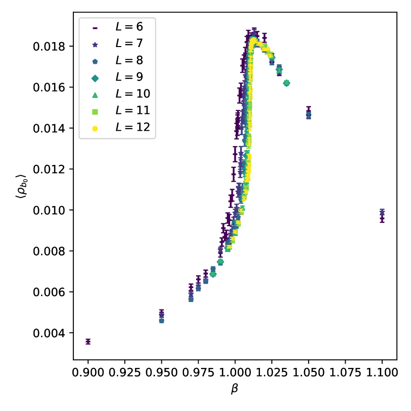
(a)

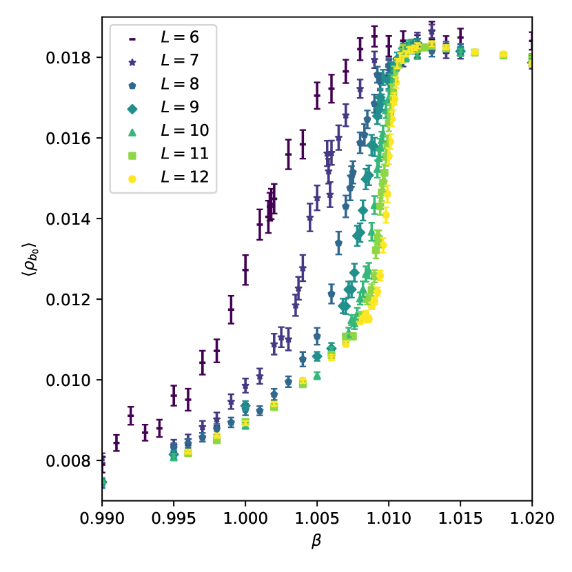
(b)

Figure 3: Scatter plots of the observable $\langle\rho_{b_{0}}\rangle$ against $\beta$ for each respective lattice size $L=\{6,...,12\}$ with error bars computed via bootstrapping with $N_{bs}=500$. In Figure 3(a), one can see that the density of networks is very low in the hot phase, increases to a maximum in the critical region and then decreases in the cold phase. In Figure 3(b), we have the same plot zoomed in around the critical region.

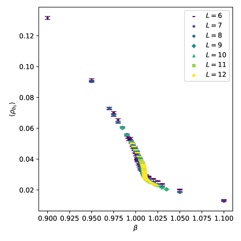
(a)

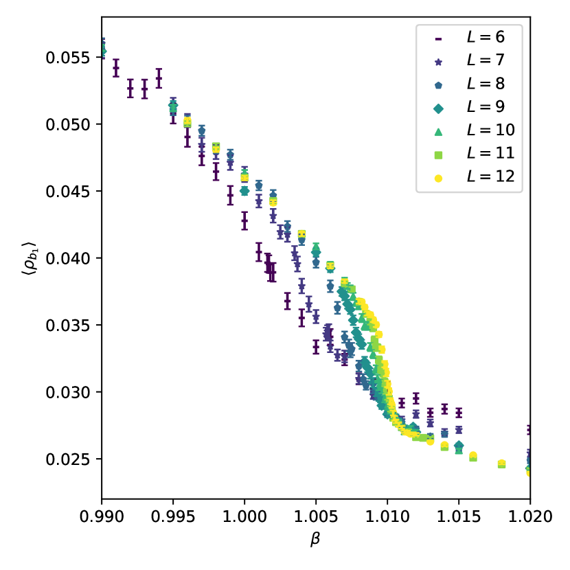
(b)

Figure 4: Scatter plots of the observable $\langle\rho_{b_{1}}\rangle$ against $\beta$ for each respective lattice size $L=\{6,...,12\}$ with error bars computed via bootstrapping with $N_{bs}=500$. As one can see, the density of loops decreases dramatically in the critical region. Again, Figure 4(b) is zoomed in around the critical region.

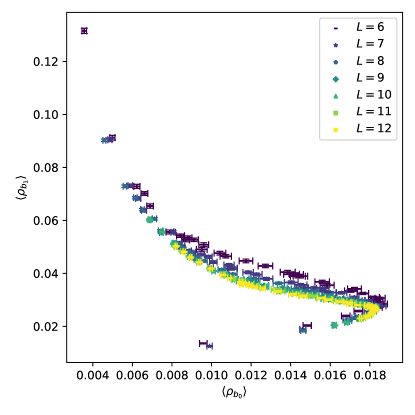
(a)

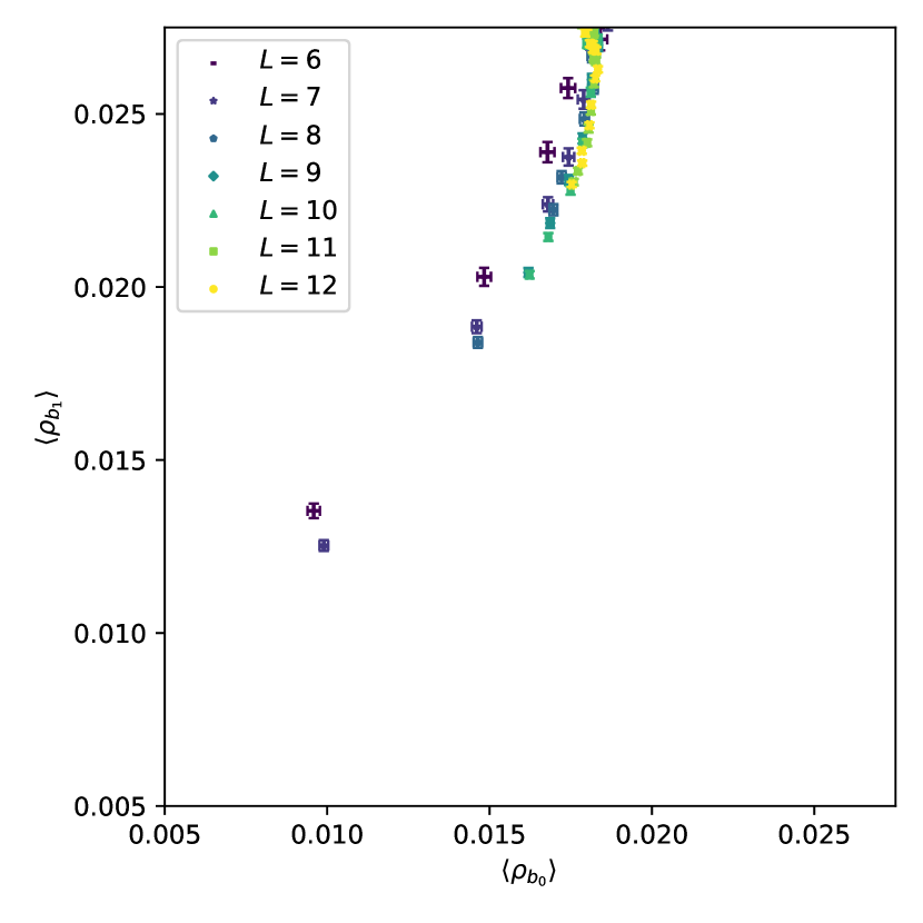
(b)

Figure 5: In Figure 5(a), we have a plot of $\langle\rho_{b_{1}}\rangle$ against $\langle\rho_{b_{0}}\rangle$ for the range $\beta\in[0.9,1.1]$ such that the top left of the plot corresponds to the hot phase, the centre of the plot corresponds to the critical region and the bottom the cold phase. In Figure 5(b), we have a zoomed in plot of the cold phase. One can see a strong positive correlation between $\rho_{b_{0}}$ and $\rho_{b_{1}}$ as one would expect for distinct, small networks.

As seen in Figure 5, we find that in the hot phase $\rho_{b_{1}}$ is negatively correlated with $\rho_{b_{0}}$ and in the cold phase $\rho_{b_{1}}$ is positively correlated with $\rho_{b_{0}}$; there exists a turning point located in the critical region. This fits with the general physical picture we expect. In the hot phase, we have a large self-intersecting, percolating network and a non-zero number of small independent networks. As the temperature increases, the size of the largest network increases; therefore, the number of self-intersections increases $\uparrow b_{1}$ and the number of distinct networks decreases $\downarrow b_{0}$. In the critical region, we have a maximum number of distinct networks as the large percolating network breaks into smaller networks. In the cold phase, we have small networks which are unlikely to self-intersect, thus $b_{1}$ evolves proportionally to $b_{0}$.

4 Conclusion and Discussion

In this paper, we have constructed two novel observables that may be used to analyse the phase structure of compact $U(1)$ lattice configurations. These are built from topological invariants of monopole current networks and we demonstrate their viability as pseudo-order parameters by showing they may be used to extract the critical inverse coupling $\beta_{c}$ such that results yield good statistical agreement with the average plaquette observable $E$. Whilst our results are an order of magnitude less precise than the literature reference $\beta_{c}$, noting our low statistics $N=200$, we do not design our methodology necessarily to achieve high precision. An advantage of our methodology is that one may probe the structure of a configuration’s monopole networks and therefore provide more evidence for a percolation-type transition of monopole currents. We claim that this provides supplementary results to [10]. In turn, we find a novel way to extract phase information from topological excitations germane to the abelian confinement mechanism in lattice gauge theories.

In order to further probe the phase structure of configurations, one might expand our analysis by using tools from TDA such as persistent homology to design more sophisticated observables, that retain a high level of interpretability, based on topological invariants of monopole current networks. This work is currently in progress and will be presented elsewhere.

Acknowledgements

The authors would like to thank Tom Pritchard for advice on optimising computational resources and Ed Bennett for feedback on the figures and the accompanying software release [57]. BL wishes to thank Claudio Bonati for discussions on the Monte Carlo update algorithm used in this work. Monte Carlo simulations were performed using software developed by Claudio Bonati with contributions from Nico Battelli, Marco Cardinali, Silvia Morlacchi and Mario Papace. Topological Data Analysis was computed using giotto-tda [58]. Histogram reweighting was computed using pymbar [59].

Author contributions

XC devised the specific methodology and performed the numerical work. BL and JG contributed equally to the formulation of the problem and devised the general methodology. All authors contributed equally to the interpretation of the results.

Funding information

XC was supported by the Additional Funding Programme for Mathematical Sciences, delivered by EPSRC (EP/V521917/1) and the Heilbronn Institute for Mathematical Research. JG was supported by EPSRC grant EP/R018472/1 through the Oxford-Liverpool-Durham Centre for Topological Data Analysis. The work of BL was partly supported by the EPSRC ExCALIBUR ExaTEPP project EP/X017168/1 and by the STFC Consolidated Grants No. ST/T000813/1 and ST/X000648/1. Numerical simulations have been performed on the Swansea SUNBIRD cluster, part of the Supercomputing Wales project. Supercomputing Wales is part funded by the European Regional Development Fund (ERDF) via Welsh Government.

Research Data Access Statement

The data shown in this manuscript can be downloaded from Ref. [60]. The code used to generate the Monte Carlo configurations and the analysis workflow used to produce the tables and the figures reported in this work can be downloaded from Ref. [57].

Open Access Statement

For the purpose of open access, the authors have applied a Creative Commons Attribution (CC BY) licence to any Author Accepted Manuscript version arising.

Appendix A Dirac Sheets

If Dirac strings pass through plaquette $\theta_{\mu\nu}(x)$, the dual plaquette $\theta_{\rho\sigma}(x)=\varepsilon_{\rho\sigma\mu\nu}\theta_{\mu\nu}(x)$ retains the same information through

$$p_{\rho\sigma}(x)=-\frac{1}{2}\varepsilon_{\rho\sigma\mu\nu}n_{\mu\nu}(x+\hat{\rho}+\hat{\sigma})\quad\in\{0,\pm 1,\pm 2\}.$$ (13)

Thus, given Equation (2.2), we have the dual relation

$$j_{\rho}(x)=\sum_{\sigma}[p_{\rho\sigma}(x)-p_{\rho\sigma}(x-\hat{\sigma})].$$ (14)

One may define a Dirac sheet $S$ as the worldsheet of a Dirac string, i.e., as a $2$-surface consisting of connected, oriented Dirac plaquettes such that $j_{\rho}(x)\neq 0$ only on the boundary $\partial S$ of the sheet, i.e., $\partial S$ is an oriented current loop. Since Dirac sheets retain information about Dirac strings, they are clearly not gauge invariant but may be classified into equivalence classes $[S]$ up to gauge transformation; $[S]$ may consequently be classified into distinct homotopy classes. If we represent $[S]$ by the sheet in the class with mininal area $S_{min}$, we may compare the minimal areas of different homotopy classes; typically, the class with the largest minimal area that spans $T^{4}$ is referred to as non-trivial.

It is worth reiterating once again that Dirac sheets are not gauge invariant. Thus, in a given configuration, it is very unlikely that the numerically determined Dirac sheets have minimal area – a necessity when classifying their gauge-equivalence classes by homotopy type for use as an order parameter. It is possible to find an equivalence class’ representative minimal area sheet $S_{min}$ via an annealing process [10]. However, this is computationally expensive and so we shall instead focus on their gauge invariant boundaries, i.e., monopole current loops.

Appendix B Methods

B.1 Histogram Reweighting

In order to achieve a more precise estimation of the critical inverse coupling $\beta_{c}$, we make use of a standard technique in lattice field theory, to produce interpolating variance curves, called histogram reweighting. Given the action of a configuration $S$, we may express the ensemble average of an observable $O$ at inverse coupling $\beta$ in terms of the ensemble average at another inverse coupling $\beta^{\prime}$ via

$$\langle O\rangle_{\beta}=\frac{\langle Oe^{-(\beta-\beta^{\prime})S}\rangle_{\beta^{\prime}}}{\langle e^{-(\beta-\beta^{\prime})S}\rangle_{\beta^{\prime}}}.$$ (15)

Regarding computational tractibility, one can only successfully reweight in regions where the distributions of the sampled actions at $\beta$ and $\beta^{\prime}$ overlap sufficiently. Multiple histogram reweighting allows us to exploit the fact that we have many sampled configurations at a range of inverse couplings. Given $N_{i}\in\mathbb{N}$ configurations each at given inverse couplings $\{\beta_{i}\}_{i=1}^{R}$ with estimated free energies $f_{\beta_{i}}$, we may reliably estimate $\langle O\rangle_{\beta}$ [61].

B.2 Bootstrap Error Estimation

In our analysis, we estimate the error via bootstrapping, i.e., resampling to estimate the standard deviation of the sampling distribution of a statistic. More precisely, given a set $S$ consisting of $N$ samples, we may compute a statistic $f(S)$. By drawing $N_{bs}$ samples from $S$ with replacement, or resampling, one may generate $N_{bs}$ new sets of samples $\{S_{i}\}_{i=1}^{N_{bs}}$ and subsequently compute the statistic $f$ on each respectively $\{f(S_{i})\}_{i=1}^{N_{bs}}$. As $N_{bs}\to\infty$, the sampling distribution of the statistic $f$ on the new bootstrapped samples $\{f(S_{i})\}$ approaches the sampling distribution of the statistic $f$ on the original set of samples $f(S)$. In our case, we would like to estimate the standard error, i.e., the standard deviation of a statistic $f$’s sampling distribution

$$\sigma_{f}\approx[\frac{1}{N_{bs}-1}\sum_{i=1}^{N_{bs}}(\,\,f(S_{i})-\langle f(S_{i})\rangle\,\,)^{2}]^{\frac{1}{2}}.$$ (16)

Appendix C Background on Homology

We give a brief review of the main ideas behind homology; then, we show how to construct the zeroth and first homology groups of a directed graph. For a more complete review, see [62].

C.1 Chain Complex

In algebraic topology, homology is a way to make precise the notion of a $k$-dimensional “hole” by way of an algebraic structure called a chain complex: given a sequence of vector spaces $\{C_{k}\}_{k=0}^{n}$ each equipped with respective boundary operator $\partial_{k}:C_{k}\to C_{k-1}$ such that $\partial_{k}\circ\partial_{k+1}\equiv 0$, then we have the chain complex

$$\cdot\cdot\cdot\xrightarrow[]{\partial_{k+1}}C_{k}\xrightarrow[]{\partial_{k}}C_{k-1}\xrightarrow[]{\partial_{k-1}}\cdot\cdot\cdot$$ (17)

The image and kernel of $\partial_{k}$ are defined as

$$\mathrm{im}\,\partial_{k} \equiv\{c^{\prime}\in C_{k-1}\,|\,\partial_{k}(c)=c^{\prime},c\in C_{k}\},$$ (18)

$$\mathrm{ker}\partial_{k} \equiv\{c\in C_{k}\,|\,\partial_{k}(c)=0\},$$ (19)

and we have that

$$\mathrm{im}\,\partial_{k+1}\subseteq\mathrm{ker}\partial_{k}.$$ (20)

We refer to elements in $\mathrm{im}\,\partial_{k+1}$ as boundaries and elements in $\mathrm{ker}\partial_{k}$ as cycles. The $k$-th homology group is the quotient group

$$H_{k}\equiv\mathrm{ker}\partial_{k}/\mathrm{im}\,\partial_{k+1}.$$ (21)

It measures the difference between these subspaces, i.e., the failure of Equation (20) to be an equality. Non-zero elements correspond to cycles that are not boundaries.

In practice, the chain complex is constructed from a geometric object such as a simplicial or cubical complex; $C_{k}$ is the vector space with basis given by the $k$-dimensional cells. In this context, the dimension of $H_{k}$ is known as the $k$-th Betti number $b_{k}$, and it counts the number of $k$-dimensional holes.

C.2 Homology of a Graph

A directed graph $X$ is defined as the tuple $(V,E)$ comprising a vertex set $V$ and an edge set $E=\{(u,v)\,|\,u,v\in V\}$ consisting of ordered pairs of vertices (c.f. a simplicial complex). From a graph, we produce a short chain complex

$$0\to C_{1}\stackrel{{\scriptstyle\partial_{1}}}{{\to}}C_{0}\to 0$$ (22)

by defining $C_{0}$ to be the vector space with basis given by the vertices, and similarly $C_{1}$ has basis given by the edges. The boundary map sends an edge $(u,v)$ to $u-v$ and is extended to all of $C_{1}$ by linearity. Note that maps into and out of the zero vector space are necessarily the zero map and thus implicit in Equation (22). We may subsequently compute the zeroth and first homology groups of the graph $X$,

$$H_{0}(X) =C_{0}/\mathrm{im}\,\partial_{1},$$

$$H_{1}(X) =\mathrm{ker}\partial_{1}.$$ (23)

For graphs, the ranks of the homology groups are independent of the choice of coefficient field. Note that in Section 3 our chosen coefficient field is $\mathbb{Z}_{2}$ for computational simplicity.

The Betti number $b_{0}(X)\equiv\dim H_{0}(X)$ is the number of connected components of the graph, and the Betti number $b_{1}(X)\equiv\dim H_{1}(X)$ is the number of loops.

Appendix D Finite-size Scaling Analysis: Further Details

In this Appendix, we provide an analysis that checks the robustness of the fit from Equation (12) by varying $k_{\text{max}}$ and the range of values. We compute the reduced chi-squared statistic $\chi^{2}_{\nu}$ as a measure of goodness of fit. We present our results for $E$, $\rho_{b_{0}}$ and $\rho_{b_{1}}$ in Table 3, Table 3 and Table 3 respectively. Our chosen fits are in bold and corresponds to the parameter choice for which $\chi^{2}_{\nu}$ takes the closest value to one.

Table 4: Finite-size scaling analysis for $E$.

Table 5: Finite-size scaling analysis for $\rho_{b_{0}}$.

Table 6: Finite-size scaling analysis for $\rho_{b_{1}}$.

References

- [1] A. M. Polyakov, Quark Confinement and Topology of Gauge Groups, Nucl. Phys. B 120, 429 (1977), 10.1016/0550-3213(77)90086-4.
- [2] S. Mandelstam, Vortices and quark confinement in non-abelian gauge theories, Physics Letters B 53(5), 476 (1975), 10.1016/0370-2693(75)90221-X.
- [3] G. Hooft, Gauge theories with unified weak, electromagnetic and strong interactions, International physics series pp. 1225–1249 (1975).
- [4] K. G. Wilson, Confinement of quarks, Phys. Rev. D 10, 2445 (1974), 10.1103/PhysRevD.10.2445.
- [5] J. Fröhlich and P. Marchetti, Soliton quantization in lattice field theories, Communications in Mathematical Physics 112, 343 (1987), 10.1007/BF01217817.
- [6] A. Di Giacomo and G. Paffuti, Disorder parameter for dual superconductivity in gauge theories, Phys. Rev. D 56, 6816 (1997), 10.1103/PhysRevD.56.6816.
- [7] T. A. DeGrand and D. Toussaint, Topological excitations and monte carlo simulation of abelian gauge theory, Phys. Rev. D 22, 2478 (1980), 10.1103/PhysRevD.22.2478.
- [8] J. S. Barber, R. E. Shrock and R. Schrader, A Study of U(1) Lattice Gauge Theory With Monopoles Removed, Phys. Lett. B 152, 221 (1985), 10.1016/0370-2693(85)91174-8.
- [9] J. S. Barber and R. E. Shrock, Dynamical Shifting of the Confinement-Deconfinement Phase Transition in 4D U(1) Lattice Gauge Theory, Nucl. Phys. B 257, 515 (1985), 10.1016/0550-3213(85)90361-X.
- [10] W. Kerler, C. Rebbi and A. Weber, Monopole currents and Dirac sheets in U(1) lattice gauge theory, Phys. Lett. B 348, 565 (1995), 10.1016/0370-2693(95)00188-Q, hep-lat/9501023.
- [11] L. Del Debbio, A. Di Giacomo and G. Paffuti, Detecting dual superconductivity in the ground state of gauge theory, Phys. Lett. B 349, 513 (1995), 10.1016/0370-2693(95)00266-N, hep-lat/9403013.
- [12] L. Di Cairano, M. Gori, M. Sarkis and A. Tkatchenko, Phase Transitions in Abelian Lattice Gauge Theory: Production and Dissolution of Monopoles and Monopole-Antimonopole Pairs (2023), 10.48550/arXiv.2303.05306.
- [13] M. Vettorazzo and P. de Forcrand, Electromagnetic fluxes, monopoles, and the order of the 4-d compact U(1) phase transition, Nucl. Phys. B 686, 85 (2004), 10.1016/j.nuclphysb.2004.02.038, hep-lat/0311006.
- [14] M. Creutz, L. Jacobs and C. Rebbi, Monte Carlo Study of Abelian Lattice Gauge Theories, Phys. Rev. D 20, 1915 (1979), 10.1103/PhysRevD.20.1915.
- [15] B. E. Lautrup and M. Nauenberg, Phase Transition in Four-Dimensional Compact QED, Phys. Lett. B 95, 63 (1980), 10.1016/0370-2693(80)90400-1.
- [16] G. Bhanot, Compact QED With an Extended Lattice Action, Nucl. Phys. B 205, 168 (1982), 10.1016/0550-3213(82)90382-0.
- [17] J. Jersak, T. Neuhaus and P. M. Zerwas, U(1) Lattice Gauge Theory Near the Phase Transition, Phys. Lett. B 133, 103 (1983), 10.1016/0370-2693(83)90115-6.
- [18] H. G. Evertz, J. Jersak, T. Neuhaus and P. M. Zerwas, Tricritical Point in Lattice QED, Nucl. Phys. B 251, 279 (1985), 10.1016/0550-3213(85)90262-7.
- [19] V. Grösch, K. Jansen, J. Jersák, C. Lang, T. Neuhaus and C. Rebbi, Monopoles and dirac sheets in compact u(1) lattice gauge theory, Physics Letters B 162(1), 171 (1985), 10.1016/0370-2693(85)91081-0.
- [20] C. B. Lang, Renormalization study of compact U(1) lattice gauge theory, Nucl. Phys. B 280, 255 (1987), 10.1016/0550-3213(87)90147-7.
- [21] C. B. Lang and T. Neuhaus, Compact U(1) gauge theory on lattices with trivial homotopy group, Nucl. Phys. B 431, 119 (1994), 10.1016/0550-3213(94)90100-7, hep-lat/9407005.
- [22] W. Kerler, C. Rebbi and A. Weber, Phase structure and monopoles in U(1) gauge theory, Phys. Rev. D 50, 6984 (1994), 10.1103/PhysRevD.50.6984, hep-lat/9403025.
- [23] W. Kerler, C. Rebbi and A. Weber, Phase transition and dynamical parameter method in U(1) gauge theory, Nucl. Phys. B 450, 452 (1995), 10.1016/0550-3213(95)00239-O, hep-lat/9503021.
- [24] J. Jersak, C. B. Lang and T. Neuhaus, NonGaussian fixed point in four-dimensional pure compact U(1) gauge theory on the lattice, Phys. Rev. Lett. 77, 1933 (1996), 10.1103/PhysRevLett.77.1933, hep-lat/9606010.
- [25] J. Jersak, C. B. Lang and T. Neuhaus, Four-dimensional pure compact U(1) gauge theory on a spherical lattice, Phys. Rev. D 54, 6909 (1996), 10.1103/PhysRevD.54.6909, hep-lat/9606013.
- [26] W. Kerler, C. Rebbi and A. Weber, Order parameters and boundary effects in U(1) lattice gauge theory, Phys. Lett. B 380, 346 (1996), 10.1016/0370-2693(96)00498-4, hep-lat/9601002.
- [27] W. Kerler, C. Rebbi and A. Weber, Critical properties and monopoles in U(1) lattice gauge theory, Phys. Lett. B 392, 438 (1997), 10.1016/S0370-2693(96)01564-X, hep-lat/9612001.
- [28] I. Campos, A. Cruz and A. Tarancon, First order signatures in 4-D pure compact U(1) gauge theory with toroidal and spherical topologies, Phys. Lett. B 424, 328 (1998), 10.1016/S0370-2693(98)00208-1, hep-lat/9711045.
- [29] I. Campos, A. Cruz and A. Tarancon, A Study of the phase transition in 4-D pure compact U(1) LGT on toroidal and spherical lattices, Nucl. Phys. B 528, 325 (1998), 10.1016/S0550-3213(98)00452-0, hep-lat/9803007.
- [30] G. Arnold, T. Lippert, K. Schilling and T. Neuhaus, Finite size scaling analysis of compact qed, Nuclear Physics B - Proceedings Supplements 94(1), 651 (2001), 10.1016/S0920-5632(01)01001-5, Proceedings of the XVIIIth International Symposium on Lattice Field Theory.
- [31] G. Arnold, B. Bunk, T. Lippert and K. Schilling, Compact qed under scrutiny: it’s first order, Nuclear Physics B - Proceedings Supplements 119, 864 (2003), 10.1016/S0920-5632(03)01704-3, Proceedings of the XXth International Symposium on Lattice Field Theory.
- [32] P. Blanchard, C. Dobrovolny, D. Gandolfo and J. Ruiz, On the mean euler characteristic and mean betti’s numbers of the ising model with arbitrary spin, Journal of Statistical Mechanics: Theory and Experiment 2006(03), P03011 (2006), 10.1088/1742-5468/2006/03/P03011.
- [33] I. Donato, M. Gori, M. Pettini, G. Petri, S. De Nigris, R. Franzosi and F. Vaccarino, Persistent homology analysis of phase transitions, Phys. Rev. E 93, 052138 (2016), 10.1103/PhysRevE.93.052138.
- [34] L. Speidel, H. A. Harrington, S. J. Chapman and M. A. Porter, Topological data analysis of continuum percolation with disks, Phys. Rev. E 98, 012318 (2018), 10.1103/PhysRevE.98.012318.
- [35] F. A. N. Santos, E. P. Raposo, M. D. Coutinho-Filho, M. Copelli, C. J. Stam and L. Douw, Topological phase transitions in functional brain networks, Phys. Rev. E 100, 032414 (2019), 10.1103/PhysRevE.100.032414.
- [36] B. Olsthoorn, J. Hellsvik and A. V. Balatsky, Finding hidden order in spin models with persistent homology, Phys. Rev. Res. 2, 043308 (2020), 10.1103/PhysRevResearch.2.043308.
- [37] Q. H. Tran, M. Chen and Y. Hasegawa, Topological persistence machine of phase transitions, Phys. Rev. E 103, 052127 (2021), 10.1103/PhysRevE.103.052127.
- [38] A. Cole, G. J. Loges and G. Shiu, Quantitative and interpretable order parameters for phase transitions from persistent homology, Phys. Rev. B 104, 104426 (2021), 10.1103/PhysRevB.104.104426.
- [39] A. Tirelli and N. C. Costa, Learning quantum phase transitions through topological data analysis, Phys. Rev. B 104, 235146 (2021), 10.1103/PhysRevB.104.235146.
- [40] N. Sale, J. Giansiracusa and B. Lucini, Quantitative analysis of phase transitions in two-dimensional models using persistent homology, Phys. Rev. E 105, 024121 (2022), 10.1103/PhysRevE.105.024121.
- [41] D. Sehayek and R. G. Melko, Persistent homology of gauge theories, Phys. Rev. B 106, 085111 (2022), 10.1103/PhysRevB.106.085111.
- [42] Y. He, S. Xia, D. G. Angelakis, D. Song, Z. Chen and D. Leykam, Persistent homology analysis of a generalized aubry-andré-harper model, Phys. Rev. B 106, 054210 (2022), 10.1103/PhysRevB.106.054210.
- [43] S. McArdle, A. Gilyén and M. Berta, A streamlined quantum algorithm for topological data analysis with exponentially fewer qubits (2022), 10.48550/arXiv.2209.12887, 2209.12887.
- [44] B. Olsthoorn, Persistent homology of quantum entanglement, Phys. Rev. B 107(11), 115174 (2023), 10.1103/PhysRevB.107.115174, 2110.10214.
- [45] H. Sun, R. K. Panda, R. Verdel, A. Rodriguez, M. Dalmonte and G. Bianconi, Network science Ising states of matter (2023), 10.48550/arXiv.2308.13604, 2308.13604.
- [46] V. Noel and D. Spitz, Detecting defect dynamics in relativistic field theories far from equilibrium using topological data analysis, Phys. Rev. D 109(5), 056011 (2024), 10.1103/PhysRevD.109.056011, 2312.04959.
- [47] D. Leykam and D. G. Angelakis, Topological data analysis and machine learning, Advances in Physics: X 8(1), 2202331 (2023), 10.1080/23746149.2023.2202331.
- [48] T. Hirakida, K. Kashiwa, J. Sugano, J. Takahashi, H. Kouno and M. Yahiro, Persistent homology analysis of deconfinement transition in effective polyakov-line model, International Journal of Modern Physics A 35(10), 2050049 (2020), 10.1142/S0217751X20500499.
- [49] K. Kashiwa, T. Hirakida and H. Kouno, Persistent homology analysis for dense qcd effective model with heavy quarks, Symmetry 14(9) (2022), 10.3390/sym14091783.
- [50] H. Antoku and K. Kashiwa, Some Aspects of Persistent Homology Analysis on Phase Transition: Examples in an Effective QCD Model with Heavy Quarks, Universe 9(2), 82 (2023), 10.3390/universe9020082.
- [51] N. Sale, B. Lucini and J. Giansiracusa, Probing center vortices and deconfinement in su(2) lattice gauge theory with persistent homology, Phys. Rev. D 107, 034501 (2023), 10.1103/PhysRevD.107.034501.
- [52] D. Spitz, J. M. Urban and J. M. Pawlowski, Confinement in non-abelian lattice gauge theory via persistent homology, Phys. Rev. D 107, 034506 (2023), 10.1103/PhysRevD.107.034506.
- [53] D. Spitz, K. Boguslavski and J. Berges, Probing universal dynamics with topological data analysis in a gluonic plasma, Phys. Rev. D 108, 056016 (2023), 10.1103/PhysRevD.108.056016.
- [54] G. Arnold, T. Lippert, K. Schilling and T. Neuhaus, Finite size scaling analysis of compact qed, Nuclear Physics B - Proceedings Supplements 94(1–3), 651–656 (2001), 10.1016/s0920-5632(01)01001-5.
- [55] K. Langfeld, B. Lucini, R. Pellegrini and A. Rago, An efficient algorithm for numerical computations of continuous densities of states, Th European Physical Journal C 76(6), 306 (2016), 10.1140/epjc/s10052-016-4142-5.
- [56] A. Bazavov and B. A. Berg, Heat bath efficiency with metropolis-type updating, Phys. Rev. D 71, 114506 (2005), 10.1103/PhysRevD.71.114506, hep-lat/0503006.
- [57] X. Crean, J. Giansiracusa and B. Lucini, Topological Data Analysis of Monopoles in Lattice Gauge Theory—Monte Carlo and analysis code release, 10.5281/zenodo.10806185 (2024).
- [58] G. Tauzin, U. Lupo, L. Tunstall, J. B. Pérez, M. Caorsi, A. M. Medina-Mardones, A. Dassatti and K. Hess, giotto-tda: : A topological data analysis toolkit for machine learning and data exploration, Journal of Machine Learning Research 22(39), 1 (2021), 10.48550/arXiv.2004.02551.
- [59] M. R. Shirts and J. D. Chodera, Statistically optimal analysis of samples from multiple equilibrium states, The Journal of chemical physics 129(12) (2008), 10.1063/1.2978177.
- [60] X. Crean, J. Giansiracusa and B. Lucini, Topological Data Analysis of Monopoles in Lattice Gauge Theory—data release, 10.5281/zenodo.10806046 (2024).
- [61] A. M. Ferrenberg and R. H. Swendsen, Optimized monte carlo data analysis, Phys. Rev. Lett. 63, 1195 (1989), 10.1103/PhysRevLett.63.1195.
- [62] H. Edelsbrunner and J. L. Harer, Computational topology: an introduction, American Mathematical Society (2022).