CAP: A General Algorithm for Online Selective Conformal Prediction with FCR Control

Abstract

We study the problem of post-selection predictive inference in an online fashion. To avoid devoting resources to unimportant units, a preliminary selection of the current individual before reporting its prediction interval is common and meaningful in online predictive tasks. Since the online selection causes a temporal multiplicity in the selected prediction intervals, it is important to control the real-time false coverage-statement rate (FCR) which measures the overall miscoverage level. We develop a general framework named CAP (Calibration after Adaptive Pick) that performs an adaptive pick rule on historical data to construct a calibration set if the current individual is selected and then outputs a conformal prediction interval for the unobserved label. We provide tractable procedures for constructing the calibration set for popular online selection rules. We proved that CAP can achieve an exact selection-conditional coverage guarantee in the finite-sample and distribution-free regimes. To account for the distribution shift in online data, we also embed CAP into some recent dynamic conformal prediction algorithms and show that the proposed method can deliver long-run FCR control. Numerical results on both synthetic and real data corroborate that CAP can effectively control FCR around the target level and yield more narrowed prediction intervals over existing baselines across various settings.

Keywords: Conformal inference, distribution-free, online prediction, selection-conditional coverage, selective inference

1 Introduction

In applications of scientific discovery or industrial production, conducting real-time selection or screening before prediction is useful because it can help allocate scarce computational or human resources to valuable individuals. Despite the high prediction accuracy of black-box models, the lack of statistical validity may hinder their participation in making further decisions. Conformal inference [Vovk et al., 1999, 2005] provides a powerful and flexible framework that can translate the prediction value from any machine learning model into a valid confidence interval. In online selective prediction problems, the validity guarantee becomes more challenging since the randomness of the real-time selection should be considered in the construction of prediction intervals (PI).

Suppose the feature-response pairs $\{Z_{t}=(X_{t},Y_{t})\}_{t\geq 0}\subseteq{\mathbb{R}}^{d}\times{\mathbb{R}}$ appear in a sequential and delayed fashion. At time $t$, we can observe the previous label $Y_{t-1}$ and the new feature $X_{t}$. Let $\Pi_{t}(\cdot):{\mathbb{R}}^{d}\to\{0,1\}$ be a generic online selection rule that may depend on the previously observed data. To be specific, we write $S_{t}=\Pi_{t}(X_{t})$ as the selection indicator, and our aim is to report the PI of the unobserved label $Y_{t}$ when $S_{t}=1$. Since training large-scale machine learning models is time-consuming, we focus on the setting that a pre-trained model $\widehat{\mu}$ is given, and we discuss the case with the online-updating learning model in Section 4. The split conformal method [Papadopoulos et al., 2002, Vovk et al., 2005] can naturally yield a marginal PI ${\mathcal{I}}_{t}^{\rm{marg}}(X_{t};\alpha)$ by computing the empirical quantile of historical residuals $\{R_{i}=|Y_{i}-\widehat{\mu}(X_{i})|\}_{i\leq t-1}$. If the data points $\{Z_{i}\}_{i\leq t}$ are i.i.d., the interval ${\mathcal{I}}_{t}^{\rm{marg}}(X_{t};\alpha)$ enjoys a distribution-free coverage guarantee ${\mathbb{P}}\left\{Y_{t}\in{\mathcal{I}}_{t}^{\rm{marg}}(X_{t};\alpha)\right\}\geq 1-\alpha$ as discussed in Lei et al. [2018].

However, due to the potential dependence between selection and prediction intervals, the multiplicity issue will arise in this setting. Benjamini and Yekutieli [2005] firstly pointed out that ignoring the multiplicity in the construction of selected parameters’ confidence intervals will lead to undesirable consequences, and they proposed the metric false coverage-statement rate (FCR) to measure the averaged miscoverage error in the constructed confidence intervals. Recently, Weinstein and Ramdas [2020] considered the temporal multiplicity and extended the definition of FCR to the online regime. For any online predictive procedure that returns intervals $\{{\mathcal{I}}_{t}(X_{t}):S_{t}=1\}_{t\geq 0}$, the corresponding FCR value and false coverage proportion (FCP) up to time $T$ are defined as

$$\operatorname{FCP}(T)=\frac{\sum_{t=0}^{T}S_{t}\cdot\mathds{1}\{Y_{t}\not\in{\mathcal{I}}_{t}(X_{t})\}}{1\vee\sum_{t=0}^{T}S_{t}},\quad\operatorname{FCR}(T)=\mathbb{E}\{\operatorname{FCP}(T)\},$$

where $a\vee b=\max\{a,b\}$ for any $a,b\in{\mathbb{R}}$. To achieve real-time FCR control when constructing post-selection confidence intervals of parameters, Weinstein and Ramdas [2020] proposed a novel approach named LORD-CI based on building marginal confidence intervals at a sequence of adjusted confidence levels $\{\alpha_{t}\}_{t\geq 0}$ such that $\sum_{t=0}^{T}\alpha_{t}/(1\vee\sum_{t=0}^{T}S_{t})\leq\alpha$ for any $T\geq 0$. The LORD-CI is a general algorithm and can readily be applicable for constructing PIs. However, as it discards the selection event when calculating the miscoverage probabilities of selected confidence intervals, the resulting PI tends to be overly wide. In fact, the paradigm of conformal prediction allows us to achieve the so-called selection-conditional coverage [Fithian et al., 2014]

$${\mathbb{P}}\left\{Y_{t}\in{\mathcal{I}}_{t}(X_{t})\mid S_{t}=1\right\}\geq 1-\alpha,\quad\forall t\geq 0,$$ (1)

under mild conditions, which characterizes the coverage property of PI conditioning on the selection event. Under some regular conditions on selection rules, the FCR can be controlled (or approximately) if the selection-conditional coverage (1) is satisfied.

1.1 Our approach: calibration after adaptive pick (CAP) on historical data

In the offline scheme, Bao et al. [2024] proposed a selective conditional conformal prediction procedure (abbreviated as SCOP) by first performing one pick rule on independent labeled data (holdout set) with the identical threshold used in the test set to construct a selected calibration set, and then constructing split conformal prediction intervals based on the empirical distribution obtained from the selected calibration set. If the threshold is invariant to the permutation of data points in the holdout set and test set, or if the threshold is an order statistic from the test set, SCOP can successfully control the FCR value around the target level. However, those assumptions about the threshold may not be realistic in the online setting where the selection rule $\Pi_{t}$ can be fully determined by previously observed data.

Motivated by the spirit of post-selection calibration in SCOP, we develop a more principled algorithm, named CAP (Calibration after Adaptive Pick) on historical data, for online selective conformal prediction. To be specific, if $S_{t}=1$ at time $t$, we firstly use a sequence of adaptive pick rules $\{\Pi_{t,s}^{\rm{Ada}}(\cdot)\}_{s\leq t-1}$ on the previously observed labeled data $\{Z_{i}\}_{i\leq t-1}$ to get a dynamic calibration set $\widehat{{\mathcal{C}}}_{t}=\{s\leq t-1:\Pi_{t,s}^{\rm{Ada}}(X_{s})=1\}$, where $\Pi_{t,s}^{\rm{Ada}}(\cdot)$ is constructed by integrating the information from the selection rules $(\Pi_{t},\Pi_{s})$ and the current feature $X_{t}$. Then for a target FCR level $\alpha$, we report the following PI:

$${\mathcal{I}}_{t}^{\rm{CAP}}(X_{t};\alpha)=\widehat{\mu}(X_{t})\pm q_{\alpha}(\{R_{i}\}_{i\in\widehat{{\mathcal{C}}}_{t}}),$$

where $q_{\alpha}(\{R_{i}\}_{i\in\widehat{{\mathcal{C}}}_{t}})$ is the $\lceil(1-\alpha)(|\widehat{{\mathcal{C}}}_{t}|+1)\rceil$-st smallest value in $\{R_{i}\}_{i\in\widehat{{\mathcal{C}}}_{t}}$.

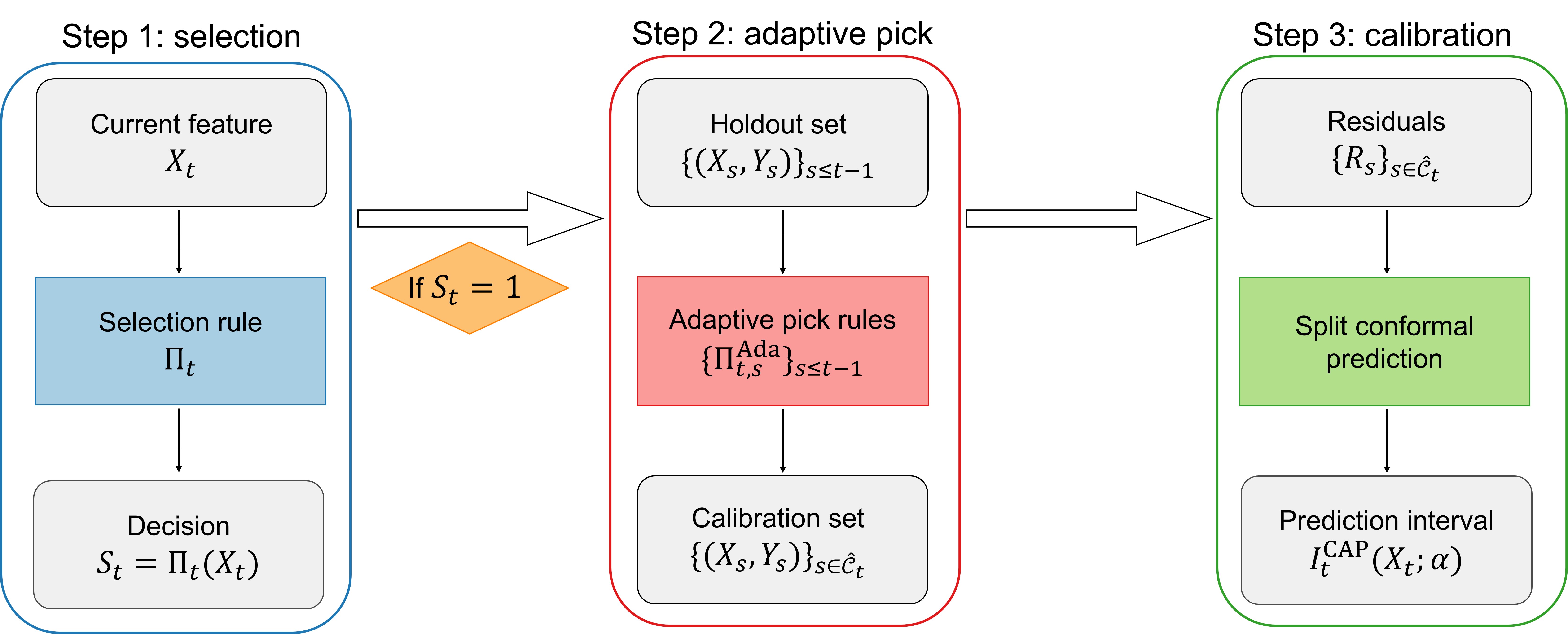
Figure 1: The workflow of CAP at time $t$. The picked calibration set is $\widehat{{\mathcal{C}}}_{t}=\left\{s\leq t-1:\Pi_{t,s}^{\rm{Ada}}(X_{s})=1\right\}$. The residuals are computed by $R_{s}=|\widehat{\mu}(X_{s})-Y_{s}|$.

To achieve the selection-conditional coverage, the adaptive pick rules $\{\Pi_{t,s}^{\rm{Ada}}(\cdot)\}_{s\leq t-1}$ are designed to guarantee the product of selection indicators $\Pi_{t,s}^{\rm{Ada}}(X_{s})\cdot S_{t}$ is symmetric with respect to the samples $(Z_{s},Z_{t})$ for $s\leq t-1$. We design adaptive pick strategies for two popular classes of selection rules to ensure exact exchangeability after selection. The first rule is the decision-driven selection considered in Weinstein and Ramdas [2020], which is broadly used in online multiple testing with false discovery rate (FDR) control [Foster and Stine, 2008, Javanmard and Montanari, 2018]. Our adaptive pick scheme takes advantage of the intrinsic property of decision-driven selection to obtain an “intersecting” subset $\widehat{{\mathcal{C}}}_{t}$. The second rule pertains to online selection with symmetric thresholds, which involves screening individuals according to the empirical distributions of historical samples. Here, we propose an adaptive pick strategy by “swapping” $X_{t}$ and $X_{i}$ for $i\leq t-1$ in the indicator $S_{t}$ to obtain a new indicator determining whether $Z_{i}$ is picked as a calibration point in $\widehat{{\mathcal{C}}}_{t}$. We show that the CAP can achieve the exact selection-conditional coverage guarantee in both pick rules.

The workflow of the proposed method CAP at time $t$ is described in Figure 1. Our contributions have four folds:

• Due to the adaptive pick in historical data, the CAP can achieve the exact selection-conditional coverage guarantee in both decision-driven selection and selection with symmetric thresholds. More importantly, our results are distribution-free and can be applied to many practical tasks without prior knowledge of data distribution.

• Compared to the offline regime, controlling the real-time FCR is more challenging due to the temporal dependence of the decisions $\{S_{t}\}_{t\geq 0}$. For decision-driven selection rules, we prove that the CAP can exactly control the real-time FCR below the target level without any distributional assumption. For the selection with symmetric thresholds, we also provide an upper bound for the real-time FCR value under certain mild stability conditions on the selection threshold. The additional error in the FCR bound will vanish to zero in the asymptotic regime in many practical settings.

• To deal with the distribution shift in online data, we adjust the level of PIs whenever the selection happens by leveraging past feedback (coverage or miscoverage) at each step. We further propose an algorithm by embedding CAP into the dynamically-tuned adaptive conformal inference (DtACI) in Gibbs and Candès [2022]. The new algorithm can achieve long-run FCR control with properly chosen parameters under arbitrary distribution shifts.

• Through extensive experiments on both synthetic and real-world data, we demonstrate the consistent superiority of our method over other benchmarks in terms of accurate FCR control and narrow PIs.

1.2 An illustrative application: drug discovery

In drug discovery, researchers examine the binding affinity of drug-target pairs on a case-by-case basis to pinpoint potential drugs with high affinity [Huang et al., 2022]. With the aid of machine learning tools, we can forecast the affinity for each drug-target pair. If the predicted affinity is high, we can select this pair for further clinical trials. To further quantify the uncertainty by predictions, our method can be employed to construct PIs with a controlled error rate.

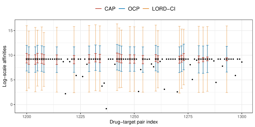
Figure 2: Plot for the real-time log-scale affinities and PIs for selected points from index 1,200 to 1,300. The selected points are marked by the cross. The PIs are constructed by three methods with a target FCR level $10\%$. Red interval: CAP (FCP at index 1,300 is $10.01\%$); Blue interval: ordinary online conformal prediction which provides marginal interval (FCP is $2.32\%$); Orange interval: LORD-CI with defaulted parameters (FCP is $0.26\%$).

Here, we apply CAP and the other two benchmarks to the DAVIS dataset [Davis et al., 2011]. The first one is the ordinary online conformal prediction (OCP), which constructs the marginal conformal intervals without consideration of the selection event. The other benchmark is LORD-CI in Weinstein and Ramdas [2020]. At each instance, we make a selection decision on a new drug-target pair. If the predicted affinity is higher than the 70% sample quantile of recent 200 predictions, the new drug-target pair is selected, and a corresponding PI is constructed. Figure 2 visualizes the real-time PIs with target FCR level $10\%$ constructed by different methods. The simulation details are provided in Section 6. Our proposed method CAP (red ones) constructs the shortest intervals with FCP at 10.01%. In contrast, both the OCP (blue ones) and the LORD-CI (orange ones) produce excessively wide intervals and yield conservative FCP levels, 2.32% and 0.26%, respectively. Therefore, the CAP emerges as a valid approach to accurately quantifying uncertainty while simultaneously achieving effective interval sizes.

1.3 Related work

Our work is closely related to the post-selection inference on parameters or labels. Benjamini and Yekutieli [2005] proposed the first method that can control FCR in finite samples by adjusting the confidence level of the marginal confidence interval. Along this path, Weinstein et al. [2013], Zhao [2022] and Xu et al. [2022] further investigated how to narrow the adjusted confidence intervals by using more useful selection information. Another line of work is the conditional approach. Fithian et al. [2014], Lee et al. [2016] and Taylor and Tibshirani [2018] proposed to construct confidence intervals for each selected variable conditional on the selection event and showed that the FCR can be further controlled if the conditional coverage property holds for an arbitrary selection subset. Those methods usually require a tractable conditional distribution given the selection condition. In particular, for the problem of online selective inference, Weinstein and Ramdas [2020] proposed a solution based on the LORD [Ramdas et al., 2017] procedure to achieve real-time FCR control for decision-driven rules. Recently, Xu and Ramdas [2023] introduced a new approach called e-LOND-CI, which utilizes e-values [Vovk and Wang, 2021] with LOND [Javanmard and Montanari, 2015] procedure for online FCR control. This method alleviates the constraints on selection rules in Weinstein and Ramdas [2020] and provides a valid FCR control under arbitrary dependence, but its setting is much different from the present one in Section 4, where we consider integrating feedback information over time.

Conformal prediction is one important brick of our proposed method. As a powerful tool for predictive inference, it provides a distribution-free coverage guarantee in both the regression [Lei et al., 2018] and the classification [Sadinle et al., 2019]. In addition to predictive intervals, conformal inference is also broadly applied to the testing problem by constructing conformal $p$-values [Bates et al., 2023, Jin and Candès, 2023a]. We refer to Angelopoulos and Bates [2021] and Shafer and Vovk [2008] for more comprehensive applications and reviews. The conventional conformal inference requires that the data points are exchangeable, which may be violated in practice. There are several works devoted to conformal inference beyond exchangeability. When the feature shift exists between the calibration set and the test set, Tibshirani et al. [2019] and Jin and Candès [2023b] introduced weighted conformal PIs and weighted conformal $p$-values, respectively, by injecting likelihood ratio weights. For general non-exchangeable data, Barber et al. [2023] used a robust weighted quantile to construct conformal PIs. For the online data under distribution shift, Gibbs and Candès [2021, 2022] developed adaptive conformal prediction algorithms based on the online learning approach. Besides, a relevant direction is to study the test-conditional coverage ${\mathbb{P}}\{Y_{t}\in{\mathcal{I}}_{t}(X_{t})\mid X_{t}=x\}$, which has been proved impossible for a finite-length PI without imposing distributional assumptions [Lei and Wasserman, 2014, Foygel Barber et al., 2021]. In contrast, our concerned selection-conditional coverage ${\mathbb{P}}\{Y_{t}\in{\mathcal{I}}_{t}(X_{t})\mid S_{t}=1\}$ could achieve reliable finite-sample guarantee without distributional assumptions.

1.4 Outline

The remainder of this paper is organized as follows. Sections 2 and 3 present the construction of the calibration set $\widehat{{\mathcal{C}}}_{t}$ and the theoretical properties of CAP for decision-driven selection and online selection with symmetric thresholds, respectively. Section 4 investigates the CAP under distribution shift. Numerical results and real-data examples are presented in Sections 5 and 6. Section 7 concludes the paper and the technical proofs are relegated to the Supplementary Material.

2 Online selective conformal prediction for decision-driven selection

Suppose a prediction model $\widehat{\mu}(\cdot):{\mathbb{R}}^{d}\to{\mathbb{R}}$ is pre-trained by an independent training set. To make sure that the PIs can be constructed when $t$ is small, we assume there exists an independent labeled set denoted by $\{Z_{i}=(X_{i},Y_{i})\}_{i=-n}^{-1}$. Let ${\mathcal{H}}_{t}=\{-n,\ldots,t-1\}$ be deterministic indices of the holdout set at time $t$. The selection rule $\Pi_{t}$ is generated from the previously observed data $\{Z_{i}\}_{i\in{\mathcal{H}}_{t}}$. We first summarize the general procedure of the online selective conformal prediction in Algorithm 1, which is abbreviated as CAP in this paper.

Algorithm 1 Calibration after Adaptive Pick (CAP) on historical data

0:  Pre-trained model $\widehat{\mu}$, initial holdout set $\{(X_{i},Y_{i})\}_{i=-n}^{-1}$, target FCR level $\alpha\in(0,1)$.

1:  Compute the residuals in the initial holdout set $\{R_{i}=|Y_{i}-\widehat{\mu}(X_{i})|\}_{i=-n}^{-1}$.

2:  for $t=0,1,\ldots$ do

3:     Observe the previous label $Y_{t-1}$ and compute its residual $R_{t-1}=|Y_{t-1}-\widehat{\mu}(X_{t-1})|$.

4:     Specify the selection rule $\Pi_{t}(\cdot)$ according to the history data $\{(X_{i},Y_{i})\}_{i\leq t-1}$.

5:     Compute the selection indicator $S_{t}=\Pi_{t}(X_{t})$.

6:     if $S_{t}=1$ then

7:        Specify the adaptive pick rules $\{\Pi_{t,s}^{\rm{Ada}}(\cdot)\}_{s\in{\mathcal{H}}_{t}}$ according to $\{(\Pi_{t},\Pi_{s},X_{t})\}_{s\in{\mathcal{H}}_{t}}$.

8:        Obtain the indices of the calibration set $\widehat{{\mathcal{C}}}_{t}=\{s\in{\mathcal{H}}_{t}:\Pi_{t,s}^{\rm{Ada}}(X_{s})=1\}$.

9:        Report the prediction interval: ${\mathcal{I}}_{t}^{\rm{CAP}}(X_{t};\alpha)=\widehat{\mu}(X_{t})\pm q_{\alpha}(\left\{R_{i}\right\}_{i\in\widehat{{\mathcal{C}}}_{t}})$.

10:     end if

11:  end for

11:  Selected PIs: $\{{\mathcal{I}}_{t}^{\rm{CAP}}(X_{t};\alpha):S_{t}=1,0\leq t\leq T\}$.

Remark 2.1.

Throughout the paper, we use the absolute residual $R(X,Y)=|Y-\widehat{\mu}(X)|$ as the nonconformity score. It is straightforward to extend Algorithm 1 to general nonconformity scores, such as quantile regression [Romano et al., 2019] or distributional regression [Chernozhukov et al., 2021]. Let $R(\cdot,\cdot):{\mathbb{R}}^{n}\times{\mathbb{R}}\to{\mathbb{R}}$ be a general nonconformity score function. We can replace the PI in Algorithm 1 with the following form

$${\mathcal{I}}_{t}^{\rm{CAP}}(X_{t};\alpha)=\left\{y\in{\mathbb{R}}:R(X_{t},y)\leq q_{\alpha}\left(\{R(X_{i},Y_{i})\}_{i\in\widehat{{\mathcal{C}}}_{t}}\right)\right\}.$$

All theoretical results in our paper will remain intact with the PIs defined above.

We will investigate the online selective conformal prediction under a class of selection rules defined below.

Definition 1.

Let $\sigma(\{S_{i}\}_{i=0}^{t-1})$ be the $\sigma$-field generated by historical decisions $\{S_{i}\}_{i=0}^{t-1}$. The online selection rule is called decision-driven selection if $\Pi_{t}(\cdot)$ is $\sigma(\{S_{i}\}_{i=0}^{t-1})$-measurable.

The decision-driven selection depends on historical data only through previous decisions. For example, one can choose $S_{t}=\mathds{1}\{\widehat{\mu}(X_{t})\leq c_{t}\}$, where $c_{t}=C_{1}+C_{2}(\sum_{i=0}^{t-1}S_{i})$ for constants $C_{1},C_{2}$. It is more flexible than choosing a constant $c_{t}\equiv C_{1}$ as the threshold since we incorporate the cumulative selection number to dynamically adjust the selection rule. Besides, many online error rate control algorithms [Foster and Stine, 2008, Aharoni and Rosset, 2014] also fall in the category of decision-driven rules, and we will discuss them in detail in Section 2.3. Before exploring the application of CAP under decision-driven selection rules, we introduce the following assumption for FCR control.

Assumption 1.

The decision-driven selection rules $\{\Pi_{t}(\cdot)\}_{t\geq 0}$ are independent of the initial holdout set $\{Z_{i}\}_{i=-n}^{-1}$.

Since the initial holdout set $\{Z_{i}\}_{i=-n}^{-1}$ is only used for calibration and the selection rule $\Pi_{t}$ depends on the previous decisions by Definition 1, Assumption 1 is reasonable for most scenarios. We notice that Weinstein and Ramdas [2020] require the confidence interval ${\mathcal{I}}_{t}(\cdot)$ to be $\sigma(\{S_{i}\}_{i=0}^{t-1})$-measurable, which means the previously observed data $\{Z_{i}\}_{i=0}^{t-1}$ cannot be used for calibration at time $t$ and the holdout set needs to be fixed as $\{Z_{i}\}_{i=-n}^{-1}$. We first regard this case as a warm-up and demonstrate that the CAP with a non-adaptive pick on the holdout set is enough to control FCR. Then in the case of the full holdout set ${\mathcal{H}}_{t}$, we show that the non-adaptive pick may fail and present a novel construction for the adaptive pick rules to select calibration data points.

2.1 Warm-up: fixed holdout set

When the holdout set is fixed as $\{Z_{i}\}_{i=-n}^{-1}$ in the entire online process, under Assumption 1, the selection indicators $\Pi_{t}(X_{t})$ and $\Pi_{t}(X_{s})$ for $-n\leq s\leq-1$ are exchangeable because $\Pi_{t}$ is independent of both $X_{t}$ and $X_{s}$. Therefore, the non-adaptive pick on the fixed holdout set is enough to guarantee the selection-conditional coverage. If $S_{t}=1$, we perform the current selection rule $\Pi_{t}$ on $\{X_{i}\}_{i=-n}^{-1}$ and obtain the following calibration candidates

$$\widehat{{\mathcal{C}}}_{t}^{\rm{fix}}=\left\{-n\leq i\leq-1:\Pi_{t}(X_{i})=1\right\}.$$

The next theorem shows that FCR can be exactly controlled below $\alpha$.

Theorem 1.

Under Assumption 1, the Algorithm 1 with $\widehat{{\mathcal{C}}}_{t}=\widehat{{\mathcal{C}}}_{t}^{\rm{fix}}$ satisfies: (1) For any $T\geq 0$, $\operatorname{FCR}(T)\leq\alpha$; (2) Let $p_{t}={\mathbb{P}}\left\{S_{t}=1\mid\sigma(\{S_{i}\}_{i=0}^{t-1})\right\}$. If the residuals $\{R_{i}\}_{i=-n}^{T}$ are distinct and $\sum_{t=0}^{T}S_{t}>0$ almost surely, we also have the following lower bound,

$$\operatorname{FCR}(T)\geq\alpha-\sum_{t=0}^{T}\mathbb{E}\left[\frac{S_{t}}{\sum_{t=0}^{T}S_{t}}\left\{\frac{1-(1-p_{t})^{n+1}}{(n+1)p_{t}}\right\}\right].$$ (2)

Theorem 1 reveals that the CAP can achieve finite-sample and distribution-free FCR control. Similar to the marginal coverage of split conformal [Lei et al., 2018], we also have the anti-conservative guarantee in (2) when the residuals are continuous. In fact, the quantity $(n+1)p_{t}$ characterizes the size of the picked calibration set $\widehat{{\mathcal{C}}}_{t}^{\rm{fix}}$. If the selection probability is bounded above zero, then the lower bound (2) becomes $\operatorname{FCR}(T)\geq\alpha-O\left\{(n+1)^{-1}\right\}$. Consequently, we have exact FCR control in the asymptotic regime, i.e., $\lim_{(n,T)\to\infty}\operatorname{FCR}(T)=\alpha$.

For completeness and comparison, we also provide the construction and validity of the online adjusted method (named LORD-CI) proposed by Weinstein and Ramdas [2020] in the conformal setting. Given any $\sigma(\{S_{i}\}_{i=0}^{t-1})$-measurable coverage level $\alpha_{t}\in(0,1)$, a marginal split conformal PI is constructed as

$${\mathcal{I}}_{t}^{\rm{marg}}(X_{t};\alpha_{t})=\widehat{\mu}(X_{t})\pm q_{\alpha_{t}}\left(\{R_{i}\}_{-n\leq i\leq-1}\right),$$ (3)

where $q_{\alpha_{t}}\left(\{R_{i}\}_{-n\leq i\leq-1}\right)$ is the $\lceil(1-\alpha_{t})(n+1)\rceil$-st smallest value in $\{R_{i}\}_{-n\leq i\leq-1}$. The PI (3) can serve as a recipe for LORD-CI by dynamically updating the marginal level $\alpha_{t}$ to maintain the following invariant

$$\frac{\sum_{t=0}^{T}\alpha_{t}}{1\vee\sum_{i=0}^{T}S_{i}}\leq\alpha,\quad\text{for any }T\geq 0.$$ (4)

We refer to Weinstein and Ramdas [2020] and literature therein for explicit procedures in constructing the sequence $\{\alpha_{t}\}_{t\geq 0}$ satisfying (4). Under the same conditions for the selection rule, we can obtain the FCR control results for LORD-CI in the conformal setting.

Proposition 1.

Let $\{S_{j}\}_{j=0}^{T}$ and $\{\widetilde{S}_{j}\}_{j=0}^{T}$ be two decision sequences, suppose $S_{t}\geq\widetilde{S}_{t}$ holds whenever $S_{j}\geq\widetilde{S}_{j}$ for any $j\leq t-1$. Under Assumption 1, if $\alpha_{t}\in\sigma(\{S_{i}\}_{i=0}^{t-1})$ for any $t\geq 0$ and the (4) holds, the LORD-CI algorithm satisfies that $\operatorname{FCR}(T)\leq\alpha$ for any $T\geq 0$.

Despite that LORD-CI can successfully control the real-time FCR, the PI ${\mathcal{I}}_{t}^{\rm{marg}}(X_{t};\alpha_{t})$ tends to be wider as $t$ grows because $\alpha_{t}$ may shrink to zero when few selections are made. The PIs of CAP will be relatively narrower due to the constant miscoverage level $\alpha$, which is also confirmed by our numerical results in Section 5.

2.2 Full holdout set

Since we can observe new labels at each time, it is more efficient to use the full holdout set $\{Z_{s}\}_{s\in{\mathcal{H}}_{t}}$ to include new labeled data points for further calibration. However, using the full holdout set results in additional dependence between the current decision $S_{t}$ and historical data $\{Z_{s}\}_{0\leq s\leq t-1}$. Typically, if we still conduct non-adaptive pick on $\{Z_{s}\}_{0\leq s\leq t-1}$ to obtain the new calibration points indexed by $\widehat{{\mathcal{C}}}_{t}^{\rm{naive}}=\{0\leq s\leq t-1:\Pi_{t}(X_{s})=1\}$, the next theorem shows that Algorithm 1 may fail in controlling FCR.

Theorem 2.

Suppose Assumption 1 holds. The Algorithm 1 with $\widehat{{\mathcal{C}}}_{t}=\widehat{{\mathcal{C}}}_{t}^{\rm{fix}}\cup\widehat{{\mathcal{C}}}_{t}^{\rm{naive}}$ satisfies that for any $T\geq 0$,

$$\operatorname{FCR}(T)\leq\alpha+\sum_{t=0}^{T}\sum_{s=0}^{t-1}\mathbb{E}\left[\frac{S_{t}}{1\vee\sum_{t=0}^{T}S_{t}}\frac{\Pi_{t}(X_{s})}{|\widehat{{\mathcal{C}}}_{t}|+1}|\Pi_{s}(X_{s})-\Pi_{s}(X_{t})|\right].$$ (5)

Notice that the product indicator $S_{t}\cdot\mathds{1}\{s\in\widehat{{\mathcal{C}}}_{t}^{\rm{naive}}\}$ for $0\leq s\leq t-1$, that is $\Pi_{t}(X_{t})\Pi_{t}(X_{s})$, has a non-symmetric dependence on the features $X_{t}$ and $X_{s}$. In fact, the selection rule $\Pi_{t}$ is independent of $X_{t}$ but relies on $\{X_{s}\}_{0\leq s\leq t-1}$ through historical decisions $\{S_{s}\}_{0\leq s\leq t-1}$. This leads to an error term in (5), which will disappear whenever $\Pi_{s}(X_{s})=\Pi_{s}(X_{t})$. An intuitive remedy is to exclude the case where the error is not zero in the construction of $\widehat{{\mathcal{C}}}_{t}$, then we consider the following intersection subset,

$$\widehat{{\mathcal{C}}}_{t}^{\text{inter}}=\widehat{{\mathcal{C}}}_{t}^{\rm{naive}}\cap\{0\leq s\leq t-1:\Pi_{s}(X_{s})=\Pi_{s}(X_{t})\}.$$

In this case, the adaptive pick rules in Algorithm 1 are chosen as $\Pi_{t,s}^{\rm{Ada}}(\cdot)=\Pi_{t}(\cdot)$ for $-n\leq s\leq-1$ and $\Pi_{t,s}^{\rm{Ada}}(\cdot)=\Pi_{t}(\cdot)\mathds{1}\{\Pi_{s}(\cdot)=\Pi_{s}(X_{t})\}$ for $0\leq s\leq t-1$.

Now let us analyze why $S_{t}\cdot\mathds{1}\{s\in\widehat{{\mathcal{C}}}_{t}^{\text{inter}}\}$ is symmetric with respective to $(X_{t},X_{s})$ for $0\leq s\leq t-1$. After expansion, we can equivalently write the product indicator as

$$S_{t}\mathds{1}\{s\in\widehat{{\mathcal{C}}}_{t}^{\text{inter}}\}=\Pi_{t}(X_{t})\Pi_{t}(X_{s})\Pi_{s}(X_{t})\Pi_{s}(X_{s})+\Pi_{t}(X_{t})\Pi_{t}(X_{s})[1-\Pi_{s}(X_{t})][1-\Pi_{s}(X_{s})].$$

Notice that if $S_{s}=1$ for $0\leq s\leq t-1$, we can replace $X_{s}$ with some $x_{s}^{*}\in\sigma(\{S_{i}\}_{i\leq s-1})$ such that $\Pi_{s}(x_{s}^{*})=1$. It will generate a sequence of virtual selection rules, denoted by $\{\widetilde{\Pi}_{j}^{(s)}\}_{j\geq s+1}$. By Definition 1, we know $\widetilde{\Pi}_{t}^{(s)}$ is identical to the real selection rule $\Pi_{t}$ under the event $\{\Pi_{s}(X_{s})=1\}$. Then the first term in $S_{t}\cdot\mathds{1}\{s\in\widehat{{\mathcal{C}}}_{t}^{\text{inter}}\}$ can be written as

$$\Pi_{t}(X_{t})\Pi_{t}(X_{s})\Pi_{s}(X_{t})\Pi_{s}(X_{s})=\widetilde{\Pi}_{t}^{(s)}(X_{t})\widetilde{\Pi}_{t}^{(s)}(X_{s})\Pi_{s}(X_{t})\Pi_{s}(X_{s}),$$

which is symmetric on $(X_{s},X_{t})$ since both $\widetilde{\Pi}_{t}^{(s)}$ and $\Pi_{s}$ are independent of $(X_{s},X_{t})$. Similarly, we can also show the second term in $S_{t}\cdot\mathds{1}\{s\in\widehat{{\mathcal{C}}}_{t}^{\text{inter}}\}$ is also symmetric on $(X_{s},X_{t})$.

Theorem 3.

Suppose Assumption 1 holds. The Algorithm 1 with $\widehat{{\mathcal{C}}}_{t}=\widehat{{\mathcal{C}}}_{t}^{\rm{fix}}\cup\widehat{{\mathcal{C}}}_{t}^{\rm{inter}}$ satisfies that (1) $\operatorname{FCR}(T)\leq\alpha$ for any $T\geq 0$; (2) ${\mathbb{P}}\left\{Y_{t}\in{\mathcal{I}}_{t}^{\rm{CAP}}(X_{t};\alpha)\mid S_{t}=1\right\}\geq 1-\alpha$ for any $t\geq 0$ when ${\mathbb{P}}(S_{t}=1)>0$.

After a modification to the picked calibration set, Algorithm 1 was guaranteed to have finite-sample and distribution-free control of FCR, as well as that of the selection-conditional coverage.

2.3 Selection with online multiple testing procedure

In this subsection, we apply the CAP to online multiple-testing problems in the framework of conformal inference. Given any user-specified thresholds $\{c_{t}\}_{t\geq 0}$, we have a sequence of hypotheses defined as

$$H_{0,t}:Y_{t}\leq c_{t},\quad\text{for }t\geq 0.$$

At time $t$, we need to make the real-time decision whether to reject $H_{0,t}$ or not. In this vein, constructing PIs for the rejected candidates is a post-selection predictive inference problem. The validity of Algorithm 1 holds with any online multiple-testing procedure that is decision-driven as Definition 1.

To control FDR in the online setting, Foster and Stine [2008] proposed firstly one method called the alpha-investing algorithm. Then Aharoni and Rosset [2014] extended it to the generalized alpha-investing (GAI) algorithm. After that, a series of works developed several variants of GAI, such as LORD, LOND  [Javanmard and Montanari, 2015], LORD++ [Ramdas et al., 2017] and SAFFRON [Ramdas et al., 2018]. Suppose we have access to a series of $p$-values $\{p_{t}\}_{t\geq 0}$, where $p_{t}$ is independent of samples in holdout set ${\mathcal{H}}_{t}$. Given the target FDR level $\beta\in(0,1)$, these procedures proceed by updating the significance level $\beta_{t}$ based on historical information and rejecting $H_{0,t}$ if $p_{t}\leq\beta_{t}$. Fortunately, all these online procedures are decision-driven selections, and CAP can naturally provide a theoretical guarantee for FCR control. Regarding the $p$-value in the framework of conformal inference, we refer to Bates et al. [2023] and Jin and Candès [2023a] for recent developments.

3 Online selection with symmetric thresholds

In the decision-driven selection rules, the influence of historical data on the current selection rule is entirely determined by past decisions. It may be inappropriate for some cases where the analyst wants to leverage the empirical distribution of historical data to select candidates. To adapt this scenario, we will rewrite the selection rule in a threshold form. Let $V(\cdot):{\mathbb{R}}^{d}\to{\mathbb{R}}$ be a user-specific or pre-trained score function used for selection, and then denote $V_{i}=V(X_{i})$ for $i\geq-n$. For ease of presentation, we rewrite the selection rule as

$$S_{t}=\Pi_{t}(X_{t})=\mathds{1}\{V_{t}\leq{\mathcal{A}}_{t}\left(\{V_{i}\}_{i\in{\mathcal{H}}_{t}}\right)\}\quad\text{for any }t\geq 0,$$ (6)

where $\{{\mathcal{A}}_{t}:{\mathbb{R}}^{t+n}\to{\mathbb{R}}\}_{t\geq 0}$ is a sequence of deterministic functions. This class of selection rules has not been studied in Weinstein and Ramdas [2020]. In particular, the selection function is assumed to have the following symmetric property.

Definition 2.

The threshold function ${\mathcal{A}}_{t}$ is symmetric if ${\mathcal{A}}_{t}(\{V_{i}\}_{i\in{\mathcal{H}}_{t}})={\mathcal{A}}_{t}(\{V_{\pi(i)}\}_{i\in{\mathcal{H}}_{t}})$ where $\pi$ is a permutation of ${\mathcal{H}}_{t}$.

For example, if $\mathcal{A}_{t}$ outputs the sample mean or sample quantile of $\{V_{i}\}_{i\in{\mathcal{H}}_{t}}$, then the corresponding selection rule $\Pi_{t}$ is symmetric. Consider the naive construction of the picked calibration set: if $S_{t}=1$, we use the same threshold to perform screening on history scores $\{V_{i}\}_{i\in{\mathcal{H}}_{t}}$, and then obtain $\widehat{{\mathcal{C}}}_{t}^{\rm{naive}}=\left\{s\in{\mathcal{H}}_{t}:V_{s}\leq{\mathcal{A}}_{t}\left(\{V_{i}\}_{i\in{\mathcal{H}}_{t}}\right)\right\}$. However, the corresponding product of selection indicators $\mathds{1}\{V_{s}\leq{\mathcal{A}}_{t}(\{V_{i}\}_{i\in{\mathcal{H}}_{t}})\}\mathds{1}\{V_{t}\leq{\mathcal{A}}_{t}(\{V_{i}\}_{i\in{\mathcal{H}}_{t}})\}$ is not symmetric with respect to $(X_{s},X_{t})$ for $s\in{\mathcal{H}}_{t}$. To construct an exchangeable selection indicator, one natural and viable solution is swapping the score from the calibration set $V_{s}$ and the score from the test set $V_{t}$ in the definition (6) of $S_{t}$, which leads to

$$\widehat{{\mathcal{C}}}_{t}^{\rm{swap}}=\left\{-n\leq s\leq t-1:V_{s}\leq{\mathcal{A}}_{t}\left(\{V_{i}\}_{i\in{\mathcal{H}}_{t},i\neq s},V_{t}\right)\right\}.$$

Hence, we may determine the adaptive pick rules in Algorithm 1 as $\Pi_{t,s}^{\rm{Ada}}(\cdot)=\mathds{1}\{V(\cdot)\leq{\mathcal{A}}_{t}\left(\{V_{i}\}_{i\in{\mathcal{H}}_{t},i\neq s},V_{t}\right)\}$. Assigning $\widehat{{\mathcal{C}}}_{t}=\widehat{{\mathcal{C}}}_{t}^{\rm{swap}}$, we can report the corresponding PI for $Y_{t}$ as stated. The next theorem guarantees that exact selection-conditional coverage can be guaranteed after swapping.

Theorem 4.

If the selection functions $\{{\mathcal{A}}_{t}\}_{t\geq 0}$ are symmetric as Definition 2, then Algorithm 1 with $\widehat{{\mathcal{C}}}_{t}=\widehat{{\mathcal{C}}}_{t}^{\rm{swap}}$ satisfies ${\mathbb{P}}\left\{Y_{t}\in{\mathcal{I}}_{t}^{\rm{CAP}}(X_{t};\alpha)\mid S_{t}=1\right\}\geq 1-\alpha$ for any $t\geq 0$ when ${\mathbb{P}}(S_{t}=1)>0$.

To control the FCR value of CAP, we impose the stability condition to bound the change of ${\mathcal{A}}_{t}$’s output after replacing $V_{s}$ with an independent copy $V$.

Assumption 2.

There exists a sequence of positive real numbers $\{\sigma_{t}\}_{t\geq 0}$ such that,

$$\max_{-n\leq s\leq t-1}\mathbb{E}\left[\big{|}{\mathcal{A}}_{t}\left(\{V_{i}\}_{i\leq t-1}\right)-{\mathcal{A}}_{t}\left(\{V_{i}\}_{i\leq t-1,i\neq s},V\right)\big{|}\mid\{V_{i}\}_{i\leq t-1,i\neq s}\right]\leq\sigma_{t},$$

where $V$ is an i.i.d. copy of $V_{s}$.

Since two sets $\{V_{i}\}_{i\leq t-1}$ and $\{V_{i}\}_{i\leq t-1,i\neq s}\cup\{V\}$ only differ one data point, the definition of $\sigma_{t}$ in Assumption 2 is similar to the global sensitivity of ${\mathcal{A}}_{t}$ in the differential privacy literature [Dwork et al., 2006].

Theorem 5.

Suppose the density function of $V_{i}$ is upper bounded by $\rho>0$. If the symmetric function ${\mathcal{A}}_{t}$ satisfies Assumption 2 for any $t\geq 0$. For Algorithm 1 with $\widehat{{\mathcal{C}}}_{t}=\widehat{{\mathcal{C}}}_{t}^{\rm{swap}}$, it holds that

$$\operatorname{FCR}(T)\leq\alpha\cdot\left\{1+\mathbb{E}\left[\frac{\mathds{1}\{\sum_{j=0}^{T}S_{j}>0\}\epsilon(T)}{\left(\sum_{j=0}^{T}S_{j}-\epsilon(T)\right)\vee 1}\right]+\frac{9}{T+n}\right\},$$ (7)

where $\epsilon(T)=2\sum_{j=0}^{T-1}\sigma_{j}+3(\sqrt{e\rho}+1)\log(T+n)+2^{-1}$.

To deal with the complicated dependence between selection and calibration, Bao et al. [2024] imposed a condition on the joint distribution for the pair of the residual and selection score $(R_{i},V_{i})$. Credited to the swapping design of $\widehat{{\mathcal{C}}}_{t}$, this assumption is no longer required in this paper. The distributional assumption on $V_{i}$ in Theorem 5 is thus quite mild.

Remark 3.1.

To analyze FCR, we need to decouple the dependence between the numerator and the denominator. The conventional leave-one-out analysis in online error rate control does not work for the selection function ${\mathcal{A}}_{t}$. In the proof of Theorem 5, we address this difficulty by using the exchangeability of data and symmetricity of ${\mathcal{A}}_{t}$. We construct a sequence of virtual decisions $\{S_{j}^{(s\leftarrow t)}\}_{j=s}^{t-1}$ by replacing $V_{s}$ with $V_{t}$ in the real decisions $\{S_{j}\}_{j=s}^{t-1}$. Since the function ${\mathcal{A}}_{j}$ is symmetric, we can guarantee that $S_{j}^{(s\leftarrow t)}$ and $S_{j}$ have the same distribution. The additional error $\epsilon(T)$ in (7) comes from the difference term $\sum_{j=s}^{t-1}S_{j}-S_{j}^{(s\leftarrow t)}$, which can be bounded via empirical Bernstein’s inequality.

Next, we will show that the error $\epsilon(T)$ can be upper bounded by a logarithmic factor with high probability when ${\mathcal{A}}_{t}$ returns the historical mean or quantile.

Proposition 2.

Suppose ${\mathcal{A}}_{t}$ returns the sample mean of history scores, i.e., $\sum_{i=-n}^{t-1}V_{i}/(t+n)$. If $\mathbb{E}[|V_{i}|]\leq\sigma$ for some $\sigma>0$, then we have $\epsilon(T)\leq 4(\sqrt{e\rho}+\sigma+1)\log(T+n)$.

Proposition 3.

Suppose ${\mathcal{A}}_{t}$ returns the $\vartheta$-th sample quantile of history scores $\{V_{i}\}_{i=-n}^{t-1}$ for $\vartheta\in(0,1]$. If $\{V_{i}\}_{i=-n}^{T}$ are continuous and $n\geq 9$, then with probability at least $1-(T+n)^{-2}$, we have $\epsilon(T)\leq 36\log^{2}(T+n)$.

Plugging the upper bounds in Propositions 2 and 3 into (7), we see that Algorithm 1 is asymptotically valid for FCR control if $\log(T+n)/(\sum_{j=0}^{T}S_{j})=o_{p}(1)$ for these two cases.

4 CAP under distribution shift

In some online settings, the exchangeable (or i.i.d.) assumption on the data generation process does not hold anymore, in which the distribution of $Z_{t}$ may vary smoothly over time. Without exchangeability, the marginal coverage cannot even be guaranteed. Gibbs and Candès [2021] developed an algorithm named adaptive conformal inference (ACI), which updates the miscoverage level according to the historical feedback on under/over coverage. For a marginal target level $\alpha$, the ACI updates the current miscoverage level by

$$\alpha_{t}=\alpha_{t-1}+\gamma\left(\alpha-\mathds{1}\{Y_{t-1}\not\in{\mathcal{I}}_{t-1}(X_{t-1};\alpha_{t-1})\}\right),$$ (8)

where $\gamma>0$ is the step size parameter. Gibbs and Candès [2022] further showed that the ACI updating rule is equivalent to a gradient descent step on the pinball loss $\ell(\theta;\beta_{t})=\alpha(\beta_{t}-\theta)-\min\{0,\beta_{t}-\theta\}$, where $\beta_{t}=\sup\{\beta\in[0,1]:Y_{t}\in{\mathcal{I}}_{t}(X_{t};\beta)\}$. That is, the miscoverage level in (8) can be written as

$$\alpha_{t}=\alpha_{t-1}-\gamma\nabla_{\theta}\ell(\alpha_{t-1};\beta_{t-1}).$$ (9)

By re-framing the ACI into an online convex optimization problem over the losses $\{\ell(\cdot;\beta_{t})\}_{t\geq 0}$, Gibbs and Candès [2022] proposed a dynamically-tuned adaptive conformal inference (DtACI) algorithm by employing an exponential reweighting scheme [Vovk, 1990, Wintenberger, 2017, Gradu et al., 2023], which can dynamically estimate the optimal step size $\gamma$.

Algorithm 2 Selective DtACI with CAP

0:  Set of candidate step-sizes $\{\gamma_{i}\}_{i=1}^{k}$, starting points $\{\alpha_{0}^{i}\}_{i=1}^{k}$, tuning parameter sequence $\{\phi_{t},\eta_{t}\}_{t=0}^{T}$.

1:  Initialize: $\tau\leftarrow\min\{t:S_{t}=1\}$, $w_{\tau}^{i}\leftarrow 1$, $p_{\tau}^{i}\leftarrow 1/k$, $\alpha_{\tau}\leftarrow\alpha_{0}^{i}$ with probability $p_{\tau}^{i}$;

2:  Call Algorithm 1 and return ${\mathcal{I}}_{\tau}^{\rm{CAP}}(X_{\tau};\alpha_{\tau})$;

3:  for $t=\tau+1,\ldots,T$ do

4:     if $S_{t}=1$ then

5:        $\beta_{\tau}\leftarrow\sup\{\beta\in[0,1]:Y_{\tau}\in{\mathcal{I}}_{\tau}^{\rm{CAP}}(X_{\tau};\beta)\}$;

6:        for $i=1,\ldots,k$ do

7:           Call Algorithm 1 and return ${\mathcal{I}}_{\tau}^{\rm{CAP}}(X_{\tau};\alpha_{\tau}^{i})$;

8:           $\operatorname{err}_{\tau}^{i}\leftarrow\mathds{1}\{Y_{\tau}\not\in{\mathcal{I}}_{\tau}^{\rm{CAP}}(X_{\tau};\alpha^{i}_{\tau})\}$;

9:           $\alpha_{t}^{i}\leftarrow\alpha_{\tau}^{i}+\gamma_{i}(\alpha-\operatorname{err}_{\tau}^{i})$;

10:           $\bar{w}_{\tau}^{i}\leftarrow w_{\tau}^{i}\exp\left\{-\eta_{\tau}\ell(\beta_{\tau},\alpha_{\tau}^{i})\right\}$;

11:        end for

12:        $w_{t}^{i}\leftarrow(1-\phi_{\tau})\bar{w}_{\tau}^{i}+\phi_{\tau}\sum_{j=1}^{k}\bar{w}_{\tau}^{j}/k$ for $1\leq i\leq k$;

13:        Define $p_{t}^{i}=w_{t}^{i}/\sum_{j=1}^{k}w_{t}^{j}$ for $1\leq i\leq k$;

14:        Assign $\alpha_{t}=\alpha_{t}^{i}$ with probability $p_{t}^{i}$;

15:        Call Algorithm 1 and return ${\mathcal{I}}_{t}^{\rm{CAP}}(X_{t};\alpha_{t})$;

16:        Set $\tau\leftarrow t$;

17:     end if

18:  end for

18:  Selected PIs: $\{{\mathcal{I}}_{t}^{\rm{CAP}}(X_{t};\alpha_{t}):S_{t}=1,0\leq t\leq T\}$.

The original motivation of ACI and DtACI is to achieve approximate marginal coverage by reactively correcting all past mistakes. For the selective inference problem, we aim to control the conditional miscoverage probability through historical feedback. In this vein, we may replace the fixed confidence level $\alpha$ in Algorithm 1 with an adapted value $\alpha_{t}$ by conditionally correcting past mistakes whenever the selection happens. If $S_{t}=1$, we firstly find the most recent selection time $\tau=\max\{0\leq s\leq t-1:S_{s}=1\}$. Define a new random variable $\beta_{\tau}^{\rm{CAP}}=\sup\{\beta\in[0,1]:Y_{\tau}\in{\mathcal{I}}_{\tau}^{\rm{CAP}}(X_{t};\alpha_{\tau})\}$. Parallel with (9), we update the current confidence level through one step of gradient descent on $\ell(\alpha_{\tau};\beta_{\tau}^{\rm{CAP}})$, i.e.,

$$\alpha_{t}=\alpha_{\tau}-\gamma\nabla_{\theta}\ell(\alpha_{\tau};\beta_{\tau}^{\rm{CAP}}).$$

Deploying the exponential reweighting scheme, we can also get a selective DtACI algorithm, and summarize it in Algorithm 2. By slightly modifying Theorem 3.2 in Gibbs and Candès [2022], we can obtain the following control result on FCR.

Theorem 6.

Let $\gamma_{\min}=\min_{i}\gamma_{i}$, $\gamma_{\max}=\max_{i}\gamma_{i}$ and $\varrho_{t}=\frac{(1+2\gamma_{\max})^{2}}{\gamma_{\min}}\eta_{t}e^{\eta_{t}(1+2\gamma_{\max})}+\frac{2(1+\gamma_{\max})}{\gamma_{\min}}\phi_{t}$. Suppose $\sum_{j=0}^{T}S_{j}>0$ almost surely. Under arbitrary distribution shift on the data $\{Z_{i}\}_{i=-n}^{T}$, Algorithm 2 satisfies that

$$\left|\operatorname{FCR}(T)-\alpha\right| \leq\frac{1+2\gamma_{\max}}{\gamma_{\min}}\mathbb{E}\left(\frac{1}{\sum_{j=0}^{T}S_{j}}\right)+\mathbb{E}\left(\frac{\sum_{t=0}^{T}S_{t}\varrho_{t}}{\sum_{j=0}^{T}S_{j}}\right),$$

where the expectation is taken over the randomness from both the data $\{Z_{i}\}_{i=-n}^{T}$ and Algorithm 2.

In Theorem 6, if $\lim_{t\to\infty}\eta_{t}=\lim_{t\to\infty}\phi_{t}=0$ and $\lim_{T\to\infty}\sum_{j=0}^{T}S_{j}=\infty$, we can guarantee $\lim_{T\to\infty}\operatorname{FCR}(T)=\alpha$. While in Gibbs and Candès [2022] advocated using constant or slowly changing values for $\eta_{t}$ to achieve approximate marginal coverage, it is more appropriate to use the decaying $\eta_{t}$ in our setting as our goal is to control the FCR value of the Algorithm 2. Despite the finite-sample guarantee no longer holds for Algorithm 2, Theorem 6 does not require any conditions on the prediction model $\widehat{\mu}$ or the online selection rule $\Pi_{t}$, which implies that Algorithm 2 is flexible in practical use. That is, we can update the learning model $\widehat{\mu}$ after observing newly labeled data to address the distribution shift.

5 Synthetic experiments

The validity and efficiency of our proposed method will be examined via extensive numerical studies. We focus on using a full holdout set, and the results for the fixed holdout set are provided in Figure S.2 of Supplementary Material. To mitigate computational costs, we adopt a windowed scheme that utilizes only the most recent 200 data points as the holdout set. Importantly, the theoretical guarantee remains intact; see the Supplementary Material for more details. Unless stated otherwise, this windowed scheme is used for all the numerical experiments.

The evaluation metrics in our experiments are empirical FCR and the average length of constructed PIs across $500$ replications. In each replication, we calculate the current FCP and the average length of all constructed intervals up to the current time $T$ and then derive the real-time FCR level and average length by averaging these values across replications.

5.1 Results for i.i.d. settings

We first generate i.i.d. 10-dimensional features $X_{i}$ from uniform distribution ${\rm Unif}([-2,2]^{10})$ and explore three distinct models for the responses $Y_{i}=\mu(X_{i})+\epsilon_{i}$ with different configurations of $\mu(\cdot)$ and distributions of $\epsilon_{i}$’s.

• Scenario A (Linear model with heterogeneous noise): Let $\mu(X)=X^{\top}\beta$ where $\beta=(\mathbf{1}_{5}^{\top},-\mathbf{1}_{5}^{\top})^{\top}$ and $\mathbf{1}_{5}$ is a $5$-dimensional vector with all elements $1$. The noise is heterogeneous and follows the conditional distribution $\epsilon\mid X\sim N(0,\{1+|\mu(X)|\}^{2})$. We employ ordinary least squares (OLS) to obtain $\hat{\mu}(\cdot)$.

• Scenario B (Nonlinear model): Let $\mu(X)=X^{(1)}+2X^{(2)}+3(X^{(3)})^{2}$, where $X^{(k)}$ denotes the $k$-th element of vector $X$ and $\epsilon\sim N(0,1)$ is independent of $X$. The support vector machine (SVM) is applied to train $\hat{\mu}(\cdot)$.

• Scenario C (Aggregation model): Let $\mu(X)=4(X^{(1)}+1)|X^{(3)}|\mathds{1}\{{X^{(2)}>-0.4}\}+4(X^{(1)}-1)\mathds{1}\{X^{(2)}\leq-0.4\}.$ The noise follows $\epsilon\sim N(0,\{1+|X^{(4)}\}))$. We use random forest (RF) to obtain $\hat{\mu}(\cdot)$.

Under each scenario, we utilize an independent labeled set with a size of 200 to train the model $\widehat{\mu}(\cdot)$. We set the initial holdout data size as $n=50$ in the simulations. The results reported in Figure F.3 of Supplementary Material show that our method CAP is not affected too much when the initial size is greater than 10.

To evaluate the performance of our proposed CAP, we conduct comprehensive comparisons with two benchmark methods. The first one is the Online Ordinary Conformal Prediction (OCP), which constructs the PI based on the whole holdout set and ignores the selection effects. The second one is the LORD-CI with default parameters as suggested in Weinstein and Ramdas [2020]. In addition, we have also considered the e-LOND-CI method proposed by Xu and Ramdas [2023]. However, our empirical studies show that it exhibits excessively conservative FCR and yields significantly wider interval lengths compared to other benchmarks. Therefore, we only included the results of this approach in Figure S.1 of Supplementary Material for reference.

Several selection rules are considered. The first is selection with a fixed threshold.

• Fixed: A selection rule with a fixed threshold is posed on the first component of the feature, i.e., $S_{t}=\mathds{1}\{X^{(1)}_{t}>1\}$. Here, we can use the naively picked calibration set $\widehat{{\mathcal{C}}}_{t}^{\rm{naive}}=\{s\in{\mathcal{H}}_{t}:\Pi_{t}(X_{s})=1\}$ for the fixed selection rule.

The next two rules are decision-driven selection in Section 2. Here, we consider the picked calibration set as $\hat{{\mathcal{C}}}^{\rm inter}_{t}$ instead of $\widehat{{\mathcal{C}}}_{t}^{\rm{naive}}$.

• Dec-driven: At each time $t$, the selection rule is $S_{t}=\mathds{1}\{\widehat{\mu}(X_{t})>\tau(\sum_{i=0}^{t-1}S_{i})\}$ where $\tau(s)=\tau_{0}-\min\{s/50,2\}$ and $\tau_{0}$ is fixed for each scenario.

• Mul-testing: Selection with the online multiple testing procedure such as SAFFRON [Ramdas et al., 2018] with defaulted parameters. We consider the hypotheses as $H_{0t}:Y_{t}\leq\tau_{0}-1$ and set the target FDR level as $\beta=20\%$. Additional independent labeled data of size $500$ is generalized to construct $p$-values. The detailed procedure is shown in the Supplementary Material.

The following two selection rules are $S_{t}=\mathds{1}\{\widehat{\mu}(X_{t})>\mathcal{A}(\{\widehat{\mu}(X_{i})\}_{i=t-200}^{t-1})\}$, which are symmetric to the holdout set. Here, we adopt $\widehat{{\mathcal{C}}}_{t}^{\rm{swap}}$ as the picked calibration set, which is defined in Section 3.

• Quantile: $\mathcal{A}(\{\widehat{\mu}(X_{i})\}_{i=t-200}^{t-1})$ is the $70\%$-quantile of the $\{\widehat{\mu}(X_{i})\}_{i=t-200}^{t-1}$.

• Mean: $\mathcal{A}(\{\widehat{\mu}(X_{i})\}_{i=t-200}^{t-1})=\sum_{i=t-200}^{t-1}\widehat{\mu}(X_{i})/200$.

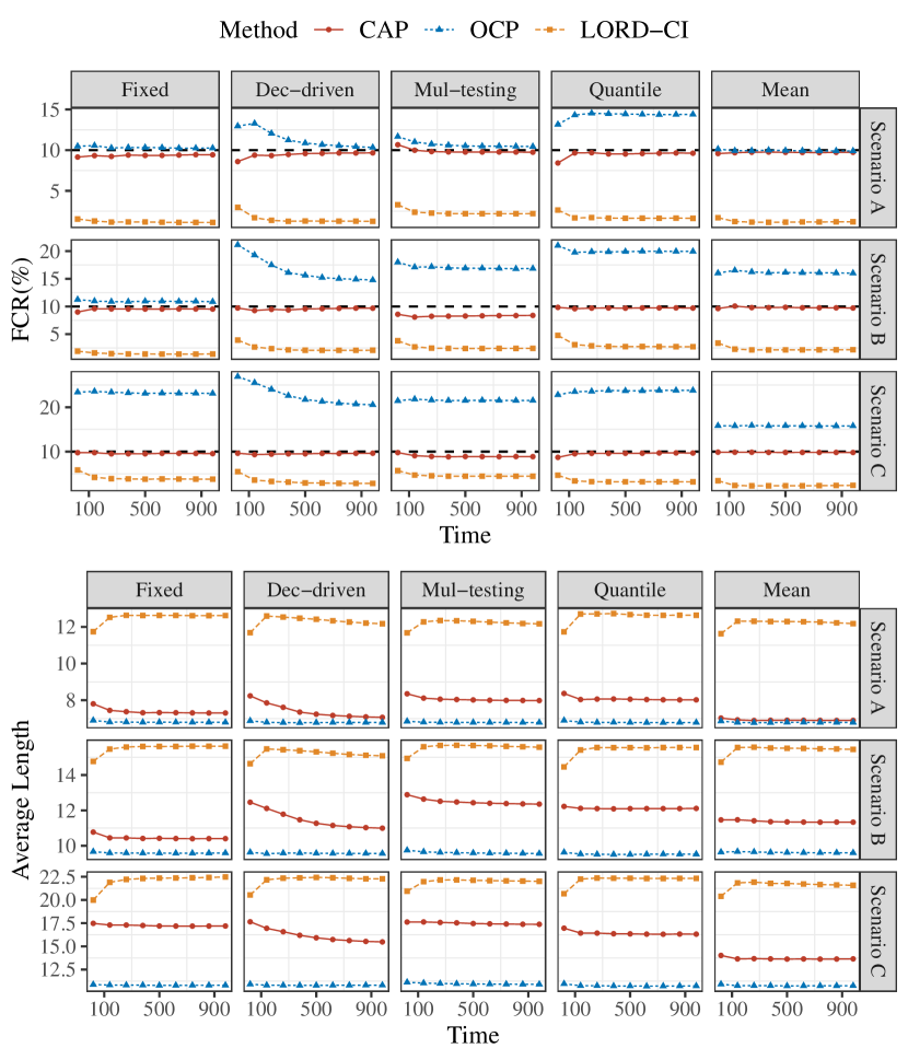
Figure 3: Real-time FCR and average length from time $20$ to $1,000$ for different scenarios and selection rules. The black dashed line denotes the target FCR level $10\%$.

Figure 3 displays the performance of all benchmarks for the full holdout set across different scenarios and selection rules. All plots indicate that the proposed CAP outperforms the other two methods uniformly in terms of real-time FCR control. This is consistent with the theoretical guarantees of CAP in FCR control. Across all settings, our method achieves stringent FCR control with narrowed PIs. As expected, the OCP yields the shortest PI lengths and much inflated FCR levels under all scenarios. This can be understood since the OCP applies all data in the holdout set to build the marginal PIs without consideration of selection effects. The LORD-CI results in considerately conservative FCR levels and accordingly it offers much wider PIs than other methods. Those unsatisfactory PIs are not surprising since the LORD-CI updates the marginal level $\alpha_{t}$ which may become small as $t$ grows, as discussed in Proposition 1.

5.2 Evaluation under distribution shift

We further consider four different settings to evaluate the performance of our proposed CAP-DtACI under distribution shifts. The first one is the i.i.d. setting which is the same as Scenario B. The second one is a slowly shifting setting where the training and initial labeled data follow the same distribution as that of Scenario B, while the online data gradually drifts over time according to $Y_{t}=(1-t/500)X_{t}^{(1)}+(2+\sin{\pi t/200})X_{t}^{(2)}+(3-t/500)(X_{t}^{(3)})^{2}+\varepsilon_{t}$, where $X_{t}\sim{\rm Unif}([-2,2])^{10}$ and $\varepsilon\sim N(0,1)$. The third is based on a change point model that generates the same data as in Scenario B when $t\leq 200$, but follows a different pattern when $t>200$, i.e., $Y_{t}=-2X_{t}^{(1)}-X_{t}^{(2)}+3(X_{t}^{(3)})^{2}+\varepsilon_{t}$ . The last shift setting is a time series model, where $Y_{t}=\{2\sin{\pi X_{t}^{(1)}X_{t}^{(2)}}+10(X_{t}^{(3)})^{2}+5X_{t}^{(4)}+2X_{t}^{(5)}+\xi_{t}\}/4$ and $\xi_{t}$ is generated from an ARMA$(0,1)$ process, specifically $\xi_{t+1}=0.99\xi_{t}+\varepsilon_{t+1}+0.99\varepsilon_{t}$.

We conducted a comparative analysis of the proposed CAP-DtACI in Algorithm 2 with the CAP in Algorithm 1, and the original DtACI. We fix the target FCR level as $\alpha=10\%$. To implement DtACI, we fix a candidate number of $k=6$, the starting points $\alpha_{0}^{i}=\alpha$ for $i=1,\cdots,6$ and determine other parameters following the suggestions in Gibbs and Candès [2022]. Typically, we consider the candidate step-sizes $\{\gamma_{i}\}_{i=1}^{6}=\{0.008,0.0160,0.032,0.064,0.128,0.256\}$ and let $\phi_{t}=\phi_{0}=1/(2I)$, $\eta_{t}=\eta_{0}=\sqrt{\{3\log(kI)+6\}/\{I(1-\alpha)^{2}\alpha^{3}+I\alpha^{2}(1-\alpha)^{2}\}}$ with $I=200$. For the proposed CAP-DtACI, we employ the same parameters except considering decaying learning parameters $\phi_{t}=\phi_{0}(\sum_{i=0}^{t}S_{t})^{-0.501}$ and $\eta_{t}=\eta_{0}(\sum_{i=0}^{t}S_{t})^{-0.501}$.

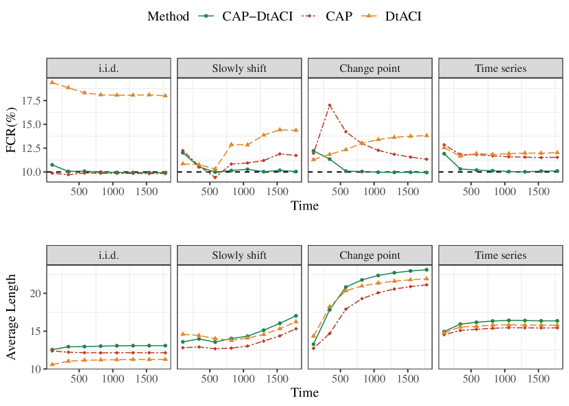
Figure 4: Comparison for CAP-DtACI, CAP and DtACI by real-time FCR and average length from time $100$ to $2,000$ for quantile selection rule under different data-generating settings. The black dashed line represents the target FCR level $10\%$.

For the sake of simplicity, we focus solely on the Quantile selection rule as previously described and leave other model settings, including the initial data size, training data size, and prediction algorithm, consistent with those in Scenario B. The results are illustrated in Figure 4. It is evident that the original DtACI consistently tends to yield an inflated FCR with respect to the target level across all four settings, as it does not account for selection effects. The CAP method can only control the FCR under the i.i.d setting, but due to the violation of exchangeability, the CAP does not work well in terms of FCR control when distribution shifts exist. In contrast, the CAP-DtACI achieves reliable FCR control across various settings by updating an adapted value $\alpha_{t}$.

6 Real data applications

6.1 Drug discovery

In Section 1.2, we consider the application of drug discovery. Here we present the details and some additional results. The DAVIS dataset [Davis et al., 2011] consists of $25,772$ drug-target pairs, each accompanied by the binding affinity, structural information of the drug compound, and the amino acid sequence of the target protein. Using the Python library DeepPurpose [Huang et al., 2020], we encode the drugs and targets into numerical features and consider the log-scale affinities as response variables. We randomly sample $15,000$ observations from the dataset as the training set to fit a small neural network model with $3$ hidden layers and 5 epochs. Additionally, we set another $2,000$ observations as the online test set, and reserve $50$ data points as the initial holdout set.

Our objective is to develop real-time prediction intervals for the affinities of selected drug-target pairs. We explore four distinct selection rules in this pursuit, including fixed selection rule $S_{t}=\mathds{1}\{\widehat{\mu}(X_{t})>9\}$; decision-driven rule with $S_{t}=\mathds{1}\{\widehat{\mu}(X_{t})>8+\min\{\sum_{j=0}^{t-1}S_{j}/400,1\}\}$; online multiple testing rule using SAFFRON, which tests $H_{0t}:Y_{t}\leq 9$ with FDR level at $20\%$ and requires another 1,000 independent labeled samples to construct conformal $p$-values; quantile selection rule, which is $S_{t}=\mathds{1}\{\widehat{\mu}(X_{t})>\mathcal{A}(\{\widehat{\mu}(X_{i})\}_{i=t-200}^{t-1})\}$, where $\mathcal{A}(\{\widehat{\mu}(X_{i})\}_{i=t-200}^{t-1})$ is the $70\%$-quantile of the $\{\widehat{\mu}(X_{i})\}_{i=t-200}^{t-1}$.

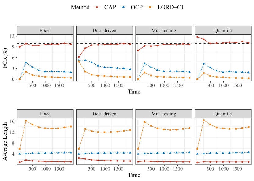
Figure 5: Real-time FCR and average length from time $20$ to $2,000$ by $50$ repetitions for drug discovery. The black dashed line denotes the target FCR level $10\%$.

Figure 5 depicts the real-time FCR and average length of PIs based on the proposed CAP, OCP and LORD-CI across $50$ runs. The results illustrate that the FCR of CAP closely aligns with the nominal level of $10\%$, and the CAP can obtain narrowed PIs over time, validating our theoretical findings. In contrast, both OCP and LORD-CI tend to yield conservative FCR values, consequently leading to unsatisfactory PI lengths. This observation is consistent with the findings presented in Figure 2, which displays the PIs of selected points when the quantile selection rule is employed. Additionally, given that the true log-scale affinities fall within the range of $(-5,10)$, excessively wide intervals would offer limited guidance for further decisions. By leveraging CAP, researchers can make informed decisions and implement reliable strategies in the pursuit of discovering promising new drugs.

6.2 Stock volatility

Stock market volatility exerts a critical role in the global financial market and trading decisions. As an indicator, forecasting future volatility in real-time can provide valuable insights for investors to make informed decisions and account for the potential risk. It is also essential to quantify the uncertainty of predicted volatility. We consider applying our proposed methods to this problem, and the time dependence would have some impact on these methods. In this task, the goal is to use the historical values of the stock price to predict the volatility the next day. Furthermore, we are concerned about the days when its predicted volatility is relatively large. Thereby, we would select those days with large predicted volatility and construct a prediction interval for them.

We consider the daily price data for NVIDIA from year 1999 to 2021. Denote the price sequence as $\{P_{t}\}_{t}$. We define the return as $X_{t}:=(P_{t}-P_{t-1})/P_{t-1}$ and the volatility as $Y_{t}=X_{t}^{2}$. At each time $t$, the predicted volatility $\hat{Y}_{t}$ is predicted by a fitted GARCH(1,1) model [Bollerslev, 1986] based on the most recent 1,250 days of returns $\{X_{i}\}_{i\leq t-1}$. And we use a normalized non-conformity score $R_{t}=|Y_{t}^{2}-\hat{Y}_{t}^{2}|/\hat{Y}^{2}_{t}$ instead of the absolute residual as Gibbs and Candès [2022] suggested. The parameters for implementing CAP-DtACI and DtACI are the same as those in Section 5.2, except that the parameter $I=1,250$. We set the FCR level $\alpha=5\%$ and use a window size of 1,250.

Four practical selection rules are considered here: fixed selection rule with $S_{t}=\mathds{1}\{\hat{Y}_{t}>8\times 10^{-4}\}$; decision-driven selection rule with $S_{t}=\mathds{1}\{\hat{Y}_{t}>8\times 10^{-4}+\min\{\sum_{j=0}^{t-1}S_{j}/50,4\}^{-4}\}$; quantile selection rule with $S_{t}=\mathds{1}\{\hat{Y}_{t}>\mathcal{A}(\{\hat{Y}_{i}\}_{i=t-1250}^{t-1})\}$ where $\mathcal{A}(\{\hat{Y}_{i}\}_{i=t-1250}^{t-1})$ is the 70%-quantile of $\{\hat{Y}_{i}\}_{i=t-1250}^{t-1}$; mean selection rule with $S_{t}=\mathds{1}\{\hat{Y}_{t}>\sum_{i=t-1250}^{t-1}\{\hat{Y}_{i}\}/1250\}$.

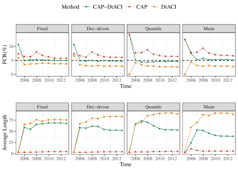
Figure 6: Real-time FCR and average length from year $2005$ to $2013$ by $20$ replications for four selection rules in stock volatility prediction task. The black dashed line denotes the target FCR level $5\%$.

Figure 6 shows the FCR and average lengths of CAP-DtACI, CAP and Dtaci over 20 replications. The replications are used to ease the randomness generated from the DtACI algorithm. As illustrated, the CAP-DtACI performs well in delivering FCR close to the target level as time grows. In contrast, the CAP has an inflated FCR due to a lack of consideration of distribution shifts and dependent structure of the time series. And the original DtACI delivers much wider PIs as it neglects the selection effects.

7 Conclusion

This paper explores the challenge of online selective inference in the context of conformal prediction. To address the non-exchangeability issue caused by the data-driven online selection process, we introduce CAP, a novel approach that could adaptively pick the calibration set from historical data to produce reliable PIs for selected observations. Our theoretical analysis and numerical experiments demonstrate the efficiency of our method in controlling FCR across diverse data environments and selection rules.

We point out several future directions. First, while our method targets two common selection rules, further exploration is needed to extend our framework to accommodate arbitrary selection rules. Second, we mainly assume a fixed predictive model for theoretical simplicity. It would be interesting to investigate the feasibility of online updating of machine learning models throughout the process for future study. Third, there may exist a more delicate variant of CAP under some special time series models to obtain tight FCR control.

Supplementary Material for “CAP: A General Algorithm for Online Selective Conformal Prediction with FCR Control”

Appendix A Preliminaries

The following two lemmas are usually used in the conformal inference literature [Vovk et al., 2005, Lei et al., 2018, Romano et al., 2019, Barber et al., 2021, 2023].

Lemma A.1.

Let $x_{(\lceil n(1-\alpha)\rceil)}$ is the $\lceil n(1-\alpha)\rceil$smallest value in $\{x_{i}\in{\mathbb{R}}:i\in[n]\}$. Then for any $\alpha\in(0,1)$, it holds that

$$\frac{1}{n}\sum_{i=1}^{n}\mathds{1}\{x_{i}>x_{(\lceil n(1-\alpha)\rceil)}\}\leq\alpha.$$

If all values in $\{x_{i}:i\in[n]\}$ are distinct, it also holds that

$$\frac{1}{n}\sum_{i=1}^{n}\mathds{1}\{x_{i}>x_{(\lceil n(1-\alpha)\rceil)}\}\geq\alpha-\frac{1}{n},$$

Lemma A.2.

Given real numbers $x_{1},...,x_{n},x_{n+1}$, let $\{x_{(r)}^{[n]}:r\in[n]\}$ be order statistics of $\{x_{i}:i\in[n]\}$, and $\{x_{(r)}^{[n+1]}:r\in[n+1]\}$ be the order statistics of $\{x_{i}:i\in[n+1]\}$, then for any $r\in[n]$ we have: $\{x_{n+1}\leq x_{(r)}^{[n]}\}=\{x_{n+1}\leq x_{(r)}^{[n+1]}\}$.

Hereafter, for any index set ${\mathcal{C}}$, we write ${\textnormal{R}}_{{\mathcal{C}}}$ as the $\lceil(1-\alpha)|{\mathcal{C}}|\rceil$st smallest value in $\{R_{i}\}_{i\in{\mathcal{C}}}$. We also omit the confidence level $\alpha$ in ${\mathcal{I}}_{t}^{\rm{CAP}}(X_{t};\alpha)$ whenever the context is clear. According to the definition of ${\mathcal{I}}_{t}^{\rm{CAP}}(X_{t})$ in Algorithm 1, together with Lemma A.2, we know

$$\mathds{1}\{Y_{t}\not\in{\mathcal{I}}_{t}^{\rm{CAP}}(X_{t})\}=\mathds{1}\{R_{t}>q_{\alpha}(\{R_{i}\}_{i\in\widehat{{\mathcal{C}}}_{t}})\}=\mathds{1}\{R_{t}>{\textnormal{R}}_{\widehat{{\mathcal{C}}}_{t}\cup\{t\}}\}.$$

In addition, Lemma A.1 guarantees

$$\alpha-\frac{1}{|\widehat{{\mathcal{C}}}_{t}|+1}\leq\frac{1}{|\widehat{{\mathcal{C}}}_{t}|+1}\sum_{j\in\widehat{{\mathcal{C}}}_{t}\cup\{t\}}\mathds{1}\{R_{j}>{\textnormal{R}}_{\widehat{{\mathcal{C}}}_{t}\cup\{t\}}\}\leq\alpha.$$

Combining the two relations above, we have the following upper bound and lower bound on the indicator of miscoverage,

$$\mathds{1}\{Y_{t}\not\in{\mathcal{I}}_{t}^{\rm{CAP}}(X_{t})\}\leq\alpha+\frac{1}{|\widehat{{\mathcal{C}}}_{t}|+1}\sum_{i\in\widehat{{\mathcal{C}}}_{t}}\left[\mathds{1}\{R_{t}>{\textnormal{R}}_{\widehat{{\mathcal{C}}}_{t}\cup\{t\}}\}-\mathds{1}\{R_{i}>{\textnormal{R}}_{\widehat{{\mathcal{C}}}_{t}\cup\{t\}}\}\right],$$ (A.1)

and

$$\mathds{1}\{Y_{t}\not\in{\mathcal{I}}_{t}^{\rm{CAP}}(X_{t})\}\geq\alpha-\frac{1}{|\widehat{{\mathcal{C}}}_{t}|+1}+\frac{1}{|\widehat{{\mathcal{C}}}_{t}|+1}\sum_{i\in\widehat{{\mathcal{C}}}_{t}}\left[\mathds{1}\{R_{t}>{\textnormal{R}}_{\widehat{{\mathcal{C}}}_{t}\cup\{t\}}\}-\mathds{1}\{R_{i}>{\textnormal{R}}_{\widehat{{\mathcal{C}}}_{t}\cup\{t\}}\}\right].$$ (A.2)

Appendix B Proofs for decision-driven selection

B.1 Proof of Theorem 1

Lemma B.1.

Denote $\delta_{t}(R_{t},R_{s})=\mathds{1}\{R_{t}>{\textnormal{R}}_{\widehat{{\mathcal{C}}}_{t}\cup\{t\}}\}-\mathds{1}\{R_{s}>{\textnormal{R}}_{\widehat{{\mathcal{C}}}_{t}\cup\{t\}}\}$. Under the conditions of Theorem 1, we have

$$\mathbb{E}\left\{\Pi_{t}(X_{t})\Pi_{t}(X_{s})\delta_{t}(R_{t},R_{s})\mid\sigma\left(\{S_{i}\}_{i=0}^{t-1},\{Z_{i}\}_{i=-n,i\neq s}^{-1}\right)\right\}=0.$$

Proof of Theorem 1.

Recall that $\widehat{{\mathcal{C}}}_{t}=\{-n\leq s\leq-1:\Pi_{t}(X_{s})=1\}$. Invoking (A.1), we can upper bound FCR by

$$\operatorname{FCR}(T) =\mathbb{E}\left[\frac{\sum_{t=0}^{T}S_{t}\mathds{1}\{Y_{t}\not\in{\mathcal{I}}_{t}^{\rm{CAP}}(X_{t})\}}{1\vee\sum_{t=0}^{T}S_{t}}\right]$$

$$\leq\sum_{t=0}^{T}\mathbb{E}\left[\frac{S_{t}}{1\vee\sum_{t=0}^{T}S_{t}}\left\{\alpha+\frac{1}{|\widehat{{\mathcal{C}}}_{t}|+1}\sum_{s\in\widehat{{\mathcal{C}}}_{t}}\delta_{t}(R_{t},R_{s})\right\}\right]$$

$$\leq\alpha+\sum_{t=0}^{T}\mathbb{E}\left[\frac{S_{t}}{1\vee\sum_{t=0}^{T}S_{t}}\frac{1}{|\widehat{{\mathcal{C}}}_{t}|+1}\sum_{s\in\widehat{{\mathcal{C}}}_{t}}\delta_{t}(R_{t},R_{s})\right].$$ (B.1)

Similarly, using (A.2), we have the following lower bound

$$\operatorname{FCR}(T) \geq\alpha-\sum_{t=0}^{T}\mathbb{E}\left[\frac{S_{t}}{1\vee\sum_{t=0}^{T}S_{t}}\frac{1}{|\widehat{{\mathcal{C}}}_{t}|+1}\right]+\sum_{t=0}^{T}\mathbb{E}\left[\frac{S_{t}}{1\vee\sum_{t=0}^{T}S_{t}}\frac{\sum_{s\in\widehat{{\mathcal{C}}}_{t}}\delta_{t}(R_{t},R_{s})}{|\widehat{{\mathcal{C}}}_{t}|+1}\right].$$ (B.2)

Let $\Pi_{j}^{(t)}(\cdot)$ be corresponding selection rule by replacing $X_{t}$ with $x_{t}^{*}\in\sigma(\{S_{i}\}_{i=0}^{t-1})$ such that $\Pi_{t}(x_{t}^{*})=1$. Correspondingly, we denote $S_{j}^{(t)}=\Pi_{j}^{(t)}(X_{j})$ for any $j\geq 0$. According to our assumption $\Pi_{t}(\cdot)\in\sigma(\{S_{i}\}_{i=0}^{t-1})$, we know: (1) $S_{j}^{(t)}=S_{j}$ for any $0\leq j\leq t-1$; (2) if $S_{t}=1$, it holds that $S_{j}^{(t)}=\Pi_{j}^{(t)}(X_{j})=\Pi_{j}(X_{j})=S_{j}$ for any $j\geq t$. Since $\Pi_{t}(\cdot)$ is independent of $\{Z_{i}\}_{i=-1}^{-n}$, we have

$$\mathbb{E}\left[\frac{S_{t}}{1\vee\sum_{t=0}^{T}S_{t}}\frac{1}{|\widehat{{\mathcal{C}}}_{t}|+1}\sum_{s\in\widehat{{\mathcal{C}}}_{t}}\delta_{t}(R_{t},R_{s})\right]$$

$$=\mathbb{E}\left[\frac{S_{t}}{1\vee\sum_{j=0}^{T}S_{j}^{(t)}}\sum_{s\in\widehat{{\mathcal{C}}}_{t}}\frac{\delta_{t}(R_{t},R_{s})}{\sum_{j=-n}^{-1}\Pi_{t}(X_{j})+1}\right]$$

$$=\mathbb{E}\left[\frac{1}{1\vee\sum_{j=0}^{T}S_{j}^{(t)}}\sum_{s=-n}^{-1}\frac{\Pi_{t}(X_{t})\Pi_{t}(X_{s})\delta_{t}(R_{t},R_{s})}{\sum_{j=-n,j\neq s}^{-1}\Pi_{t}(X_{j})+2}\right]$$

$$=\mathbb{E}\left[\frac{1}{1\vee\sum_{j=0}^{T}S_{j}^{(t)}}\sum_{s=-n}^{-1}\frac{\mathbb{E}\left\{\Pi_{t}(X_{t})\Pi_{t}(X_{s})\delta_{t}(R_{t},R_{s})\mid\sigma\left(\{S_{i}\}_{i=0}^{t-1},\{Z_{i}\}_{i=t+1}^{T},\{Z_{i}\}_{i=-n,i\neq s}^{-1}\right)\right\}}{\sum_{j=-n,j\neq s}^{-1}\Pi_{t}(X_{j})+2}\right]$$

$$=\mathbb{E}\left[\frac{1}{1\vee\sum_{j=0}^{T}S_{j}^{(t)}}\sum_{s=-n}^{-1}\frac{\mathbb{E}\left\{\Pi_{t}(X_{t})\Pi_{t}(X_{s})\delta_{t}(R_{t},R_{s})\mid\sigma\left(\{S_{i}\}_{i=0}^{t-1},\{Z_{i}\}_{i=-n,i\neq s}^{-1}\right)\right\}}{\sum_{j=-n,j\neq s}^{-1}\Pi_{t}(X_{j})+2}\right]$$

$$=0,$$ (B.3)

where the last equality follows from Lemma B.1. Plugging (B.1) into (B.1) gives the desired upper bound $\operatorname{FCR}(T)\leq\alpha$. Let $p_{t}={\mathbb{P}}\left\{\Pi_{t}(X_{t})=1\mid\sigma(\{S_{i}\}_{i=0}^{t-1})\right\}$. From the i.i.d. assumption, we know $|\widehat{{\mathcal{C}}}_{t}|\sim\operatorname{Binomial}(n,p_{t})$ given $\sigma(\{S_{i}\}_{i=0}^{t-1})$. Then we have

$$\mathbb{E}\left[\frac{S_{t}}{1\vee\sum_{t=0}^{T}S_{t}}\frac{1}{|\widehat{{\mathcal{C}}}_{t}|+1}\right] =\mathbb{E}\left[\frac{1}{1+\sum_{j\neq t}^{T}S_{j}}\mathbb{E}\left\{\frac{S_{t}}{|\widehat{{\mathcal{C}}}_{t}|+1}\mid\sigma(\{S_{i}\}_{i=0}^{t-1}),\{Z_{i}\}_{i\geq t+1}\right\}\right]$$

$$\stackrel{{\scriptstyle(i)}}{{=}}\mathbb{E}\left[\frac{1}{1+\sum_{j\neq t}^{T}S_{j}}\mathbb{E}\left\{\frac{S_{t}}{|\widehat{{\mathcal{C}}}_{t}|+1}\mid\sigma(\{S_{i}\}_{i=0}^{t-1})\right\}\right]$$

$$\stackrel{{\scriptstyle(ii)}}{{=}}\mathbb{E}\left[\frac{1}{1+\sum_{j\neq t}^{T}S_{j}}\mathbb{E}\left\{S_{t}\mid\sigma(\{S_{i}\}_{i=0}^{t-1})\right\}\cdot\mathbb{E}\left\{\frac{1}{|\widehat{{\mathcal{C}}}_{t}|+1}\mid\sigma(\{S_{i}\}_{i=0}^{t-1})\right\}\right]$$

$$=\mathbb{E}\left[\frac{1}{1+\sum_{j\neq t}^{T}S_{j}}\mathbb{E}\left\{S_{t}\mid\sigma(\{S_{i}\}_{i=0}^{t-1})\right\}\cdot\frac{1-(1-p_{t})^{n+1}}{(n+1)p_{t}}\right]$$

$$=\mathbb{E}\left[\frac{S_{t}}{1\vee\sum_{j=0}^{T}S_{j}}\frac{1-(1-p_{t})^{n+1}}{(n+1)p_{t}}\right],$$ (B.4)

where $(i)$ holds since $S_{t},|\widehat{{\mathcal{C}}}_{t}|\mathop{\perp\!\!\!\perp}\{Z_{i}\}_{i\geq t+1}$ given $\sigma(\{S_{i}\}_{i=0}^{t-1})$; and $(ii)$ holds due to i.i.d. assumption. Plugging (B.1) and (B.1) into (B.2) yields the desired lower bound

$$\operatorname{FCR}(T) \geq\alpha\cdot\mathbb{E}\left[\frac{\sum_{t=0}^{T}S_{t}}{1\vee\sum_{j=0}^{T}S_{j}}\right]-\sum_{t=0}^{T}\mathbb{E}\left[\frac{S_{t}}{1\vee\sum_{j=0}^{T}S_{j}}\frac{1-(1-p_{t})^{n+1}}{(n+1)p_{t}}\right]$$

$$=\alpha-\sum_{t=0}^{T}\mathbb{E}\left[\frac{S_{t}}{\sum_{j=0}^{T}S_{j}}\frac{1-(1-p_{t})^{n+1}}{(n+1)p_{t}}\right],$$

where the last inequality follows from the assumption $\sum_{j=0}^{T}S_{j}>0$ with probability 1. Therefore, we have finished the proof. ∎

B.2 Proof of Lemma B.1

Proof.

We first notice that $\Pi_{t}(\cdot)$ is fixed given $\sigma(\{S_{i}\}_{i=0}^{t-1})$. It also means that $\{\Pi_{t}(X_{-i})\}_{i=1,i\neq s}^{n}$ are also fixed given $\sigma(\{S_{i}\}_{i=0}^{t-1},\{Z_{i}\}_{i=-n,i\neq s}^{-1})$. Let $z_{1}=(x_{1},y_{1})$ and $z_{2}=(x_{2},y_{2})$. Now define the event ${\mathcal{E}}_{z}=\left\{[Z_{s},Z_{t}]=[z_{1},z_{2}]\right\}$, where $[Z_{s},Z_{t}]$ and $[z_{1},z_{2}]$ are two unordered sets. Clearly, we know ${\textnormal{R}}_{\widehat{{\mathcal{C}}}_{t}\cup\{t\}}$ is fixed given ${\mathcal{E}}_{z}$ and $\sigma(\{S_{i}\}_{i=0}^{t-1},\{Z_{i}\}_{i=-n,i\neq s}^{-1})$. Recalling the definition of $\delta_{t}(R_{t},R_{s})$, we can get

$$\mathbb{E}\left[\Pi_{t}(X_{t})\Pi_{t}(X_{s})\delta_{t}(R_{t},R_{s})\mid\sigma\left(\{S_{i}\}_{i=0}^{t-1},\{Z_{i}\}_{i=-n,i\neq s}^{-1}\right),{\mathcal{E}}_{z}\right]$$

$$\qquad={\mathbb{P}}\left\{R_{t}>{\textnormal{R}}_{\widehat{{\mathcal{C}}}_{t}\cup\{t\}},\Pi_{t}(X_{t})=1,\Pi_{t}(X_{s})=1\mid\sigma\left(\{S_{i}\}_{i=0}^{t-1},\{Z_{i}\}_{i=-n,i\neq s}^{-1}\right),{\mathcal{E}}_{z}\right\}$$

$$\qquad-{\mathbb{P}}\left\{R_{s}>{\textnormal{R}}_{\widehat{{\mathcal{C}}}_{t}\cup\{t\}},\Pi_{t}(X_{t})=1,\Pi_{t}(X_{s})=1\mid\sigma\left(\{S_{i}\}_{i=0}^{t-1},\{Z_{i}\}_{i=-n,i\neq s}^{-1}\right),{\mathcal{E}}_{z}\right\}$$

$$\qquad\stackrel{{\scriptstyle(*)}}{{=}}\frac{1}{2}\mathds{1}\{\Pi_{t}(x_{1})=1,\Pi_{t}(x_{2})=1\}\left[\mathds{1}\{r_{1}>{\textnormal{R}}_{\widehat{{\mathcal{C}}}_{t}\cup\{t\}}\}+\mathds{1}\{r_{2}>{\textnormal{R}}_{\widehat{{\mathcal{C}}}_{t}\cup\{t\}}\}\right]$$

$$\qquad-\frac{1}{2}\mathds{1}\{\Pi_{t}(x_{1})=1,\Pi_{t}(x_{2})=1\}\left[\mathds{1}\{r_{1}>{\textnormal{R}}_{\widehat{{\mathcal{C}}}_{t}\cup\{t\}}\}+\mathds{1}\{r_{2}>{\textnormal{R}}_{\widehat{{\mathcal{C}}}_{t}\cup\{t\}}\}\right]$$

$$\qquad=0,$$

where $r_{1}=|y_{1}-\widehat{\mu}(x_{1})|$ and $r_{2}=|y_{2}-\widehat{\mu}(x_{2})|$; the equality $(*)$ holds since $(R_{s},R_{t})$ are exchangeable and ${\mathcal{E}}_{z}\mathop{\perp\!\!\!\perp}(\{S_{i}\}_{i=0}^{t-1},\{Z_{i}\}_{i=-n,i\neq s}^{-1})$. Through marginalizing over ${\mathcal{E}}_{z}$, we can prove the desired result. ∎

B.3 Proof of Proposition 1

Proof.

Recall that ${\mathcal{I}}_{t}^{\rm{marg}}(X_{t};\alpha_{t})=\widehat{\mu}(X_{t})\pm q_{\alpha_{t}}\left(\{R_{i}\}_{i\in{\mathcal{H}}_{0}}\right)$ with ${\mathcal{H}}_{0}=\{-n,\ldots,-1\}$. It follows that

$$\mathds{1}\{Y_{t}\not\in{\mathcal{I}}_{t}^{\rm{marg}}(X_{t};\alpha_{t})\}\leq\alpha_{t}+\frac{1}{n+1}\sum_{s=-n}^{-1}\delta_{t}(R_{t},R_{s}),$$ (B.5)

where $\delta_{t}(R_{t},R_{s})=\mathds{1}\{R_{t}>{\textnormal{R}}_{{\mathcal{H}}_{0}\cup\{t\}}\}-\mathds{1}\{R_{s}>{\textnormal{R}}_{{\mathcal{H}}_{0}\cup\{t\}}\}$. We follow the notation $S_{j}^{(t)}$ in Section B.1. By the definition, we have

$$\operatorname{FCR}(T) =\sum_{t=0}^{T}\mathbb{E}\left[\frac{S_{t}\mathds{1}\{Y_{t}\not\in{\mathcal{I}}_{t}^{\rm{marg}}(X_{t};\alpha_{t})\}}{1\vee\sum_{j=0}^{T}S_{j}}\right]$$

$$=\sum_{t=0}^{T}\mathbb{E}\left[\frac{S_{t}\mathds{1}\{Y_{t}\not\in{\mathcal{I}}_{t}^{\rm{marg}}(X_{t};\alpha_{t})\}}{1\vee\sum_{j=0}^{T}S_{j}^{(t)}}\right]$$

$$\leq\sum_{t=0}^{T}\mathbb{E}\left[\frac{\mathds{1}\{Y_{t}\not\in{\mathcal{I}}_{t}^{\rm{marg}}(X_{t};\alpha_{t})\}}{1\vee\sum_{j=0}^{T}S_{j}^{(t)}}\right]$$

$$\stackrel{{\scriptstyle(i)}}{{\leq}}\sum_{t=0}^{T}\mathbb{E}\left[\frac{\alpha_{t}}{1\vee\sum_{j=0}^{T}S_{j}^{(t)}}\right]+\sum_{t=0}^{T}\mathbb{E}\left[\frac{1}{1\vee\sum_{j=0}^{T}S_{j}^{(t)}}\frac{\sum_{s=-n}^{-1}\delta_{t}(R_{t},R_{s})}{n+1}\right]$$

$$\stackrel{{\scriptstyle(ii)}}{{\leq}}\alpha+\sum_{t=0}^{T}\mathbb{E}\left[\mathbb{E}\left\{\frac{1}{1\vee\sum_{j=0}^{T}S_{j}^{(t)}}\frac{\sum_{s=-n}^{-1}\delta_{t}(R_{t},R_{s})}{n+1}\mid\sigma\left(\{S_{i}\}_{i=0}^{t-1}\right)\right\}\right]$$

$$\stackrel{{\scriptstyle(iii)}}{{\leq}}\alpha+\sum_{t=0}^{T}\mathbb{E}\left[\mathbb{E}\left\{\frac{1}{1\vee\sum_{j=0}^{T}S_{j}^{(t)}}\mid\sigma\left(\{S_{i}\}_{i=0}^{t-1}\right)\right\}\frac{\sum_{s=-n}^{-1}\mathbb{E}\left[\delta_{t}(R_{t},R_{s})\mid\sigma\left(\{S_{i}\}_{i=0}^{t-1}\right)\right]}{n+1}\right]$$

$$\stackrel{{\scriptstyle(iv)}}{{=}}\alpha,$$

where $(i)$ follows from (B.5); $(ii)$ holds due to the LORD-CI’s invariant $\sum_{t=0}^{T}\alpha_{t}/(\sum_{j=0}^{T}S_{j})\leq\alpha$ and $S_{j}^{(t)}\geq S_{j}$ for any $j\geq t$; $(iii)$ holds since $\alpha_{t}\in\sigma\left(\{S_{i}\}_{i=0}^{t-1}\right)$ and $(Z_{t},Z_{s})\mathop{\perp\!\!\!\perp}S_{j}^{(t)}$ for $j\geq t$; and $(iv)$ follows from the exchangeability between $Z_{t}$ and $Z_{s}$ such that

$$\mathbb{E}\left[\delta_{t}(R_{t},R_{s})\mid\sigma\left(\{S_{i}\}_{i=0}^{t-1}\right)\right] =\mathbb{E}\left[\delta_{t}(R_{t},R_{s})\right]$$

$$={\mathbb{P}}\left(R_{t}>{\textnormal{R}}_{{\mathcal{H}}_{0}\cup\{t\}}\right)-{\mathbb{P}}\left(R_{s}>{\textnormal{R}}_{{\mathcal{H}}_{0}\cup\{t\}}\right)=0.$$

∎

B.4 Proof of Theorem 2

Proof.

Recall that $\widehat{{\mathcal{C}}}_{t}=\{i\leq t-1:\Pi_{t}(X_{i})=1\}$. Similar to (B.1), we can show

$$\sum_{s=-n}^{-1}\mathbb{E}\left[\frac{1}{1\vee\sum_{j=0}^{T}S_{j}}\frac{1}{|\widehat{{\mathcal{C}}}_{t}|+1}\Pi_{t}(X_{t})\Pi_{t}(X_{s})\delta_{t}(R_{t},R_{s})\right]=0,$$ (B.6)

Let $x_{s,1},x_{s,0}\in\sigma(S_{0},\ldots,S_{s-1})$ be the values such that $\Pi_{s}(x_{s,1})=1$ and $\Pi_{s}(x_{s,0})=0$ for $0\leq s\leq t-1$. Denote $\{\Pi_{i}^{(s,1)}\}_{i\geq 0}$ and $\{\Pi_{i}^{(s,0)}\}_{i\geq 0}$ the virtual selection rules generated by replacing $X_{s}$ with $x_{s,1}$ and $x_{s,0}$, respectively. Let $\{S_{i}^{(s,1)}\}_{i\geq 0}$ and $\{S_{i}^{(s,0)}\}_{i\geq 0}$ be the corresponding virtual decision sequences. In addition, we define

$$\widehat{{\mathcal{C}}}_{i}^{(s,1)}=\left\{-n\leq j\leq-1:\Pi_{i}(X_{j})=1\right\}\cup\left\{0\leq j\leq t-1:\Pi_{i}^{(s,1)}(X_{j})=1\right\},$$

$$\widehat{{\mathcal{C}}}_{i}^{(s,0)}=\left\{-n\leq j\leq-1:\Pi_{i}(X_{j})=1\right\}\cup\left\{0\leq j\leq t-1:\Pi_{i}^{(s,0)}(X_{j})=1\right\}.$$

Further, we denote

$$\delta_{t}^{(s,1)}(R_{t},R_{s})=\mathds{1}\{R_{t}>{\textnormal{R}}_{\widehat{{\mathcal{C}}}_{t}^{(s,1)}\cup\{t\}}\}-\mathds{1}\{R_{s}>{\textnormal{R}}_{\widehat{{\mathcal{C}}}_{t}^{(s,1)}\cup\{t\}}\},$$

$$\delta_{t}^{(s,0)}(R_{t},R_{s})=\mathds{1}\{R_{t}>{\textnormal{R}}_{\widehat{{\mathcal{C}}}_{t}^{(s,0)}\cup\{t\}}\}-\mathds{1}\{R_{s}>{\textnormal{R}}_{\widehat{{\mathcal{C}}}_{t}^{(s,0)}\cup\{t\}}\}.$$

Then we have the following conclusions:

• $\Pi_{i}^{(s,1)}=\Pi_{i}$ and $\widehat{{\mathcal{C}}}_{i}^{(s,1)}=\widehat{{\mathcal{C}}}_{i}^{(s,0)}=\widehat{{\mathcal{C}}}_{i}$ for any $i\leq s$;

• If $S_{s}=1$, then $\Pi_{i}^{(s,1)}=\Pi_{i}$, $\widehat{{\mathcal{C}}}_{i}^{(s,1)}=\widehat{{\mathcal{C}}}_{i}$ for any $i\geq s+1$ and $\delta_{t}^{(s,1)}(R_{t},R_{s})=\delta_{t}(R_{t},R_{s})$.

• If $S_{s}=0$, then $\Pi_{i}^{(s,0)}=\Pi_{i}$, $\widehat{{\mathcal{C}}}_{i}^{(s,0)}=\widehat{{\mathcal{C}}}_{i}$ for any $i\geq s+1$ and $\delta_{t}^{(s,0)}(R_{t},R_{s})=\delta_{t}(R_{t},R_{s})$.

Let $x_{t}^{(s,1)}\in\sigma(S_{0,1}^{(s)},\ldots,S_{t-1,1}^{(s)})$ and $x_{t}^{(s,0)}\in\sigma(S_{0,0}^{(s)},\ldots,S_{t-1,0}^{(s)})$ be the values such that $\Pi_{t}^{(s,1)}(x_{t}^{(s,1)})=1$ and $\Pi_{t}^{(s,0)}(x_{t}^{(s,0)})=1$ for $t>s$, respectively. Let $\{S_{i,1}^{(s,t)}\}_{i\geq 0}$ be the virtual decision sequence generated by firstly replacing $X_{s}$ with $x_{s,1}$, and then replacing $X_{t}$ with $x_{t}^{(s,1)}$. Let $\{S_{i,0}^{(s,t)}\}_{i\geq 0}$ be the virtual decision sequence generated by firstly replacing $X_{s}$ with $x_{s,0}$, and then replacing $X_{t}$ with $x_{t}^{(s,1)}$. In this case, we can guarantee that $S_{i,1}^{(s,t)},S_{i,0}^{(s,t)}\mathop{\perp\!\!\!\perp}(Z_{s},Z_{t})$ for any $i\geq 0$ because $x_{s,1},x_{s,0}\mathop{\perp\!\!\!\perp}(Z_{s},Z_{t})$ and $x_{t}^{(s,1)},x_{t}^{(s,0)}\mathop{\perp\!\!\!\perp}(Z_{s},Z_{t})$. We have

• $S_{i,1}^{(s,t)}=S_{i,0}^{(s,t)}=S_{i}$ for $i\leq s-1$;

• $S_{i,1}^{(s,t)}=S_{i}^{(s,1)}$ and $S_{i,0}^{(s,t)}=S_{i}^{(s,0)}$ for $s\leq i\leq t-1$;

• If $S_{t}=1$, $S_{i,1}^{(s,t)}=S_{i}^{(s,1)}$ for $i\geq t$.

• If $S_{t}=0$, $S_{i,0}^{(s,t)}=S_{i}^{(s,0)}$ for $i\geq t$.

For any pair $(s,t)$ with $0\leq s\leq t-1$, we denote

$$H_{s,t}(X_{s},X_{t}) =\Pi_{t}(X_{s})\Pi_{s}(X_{t})\Pi_{s}(X_{s}),$$

$$H_{s,t}^{(s,1)}(X_{s},X_{t}) =\Pi_{t}^{(s,1)}(X_{s})\Pi_{s}(X_{t})\Pi_{s}(X_{s}),$$

$$J_{s,t}(X_{s},X_{t}) =\Pi_{t}(X_{s})[1-\Pi_{s}(X_{s})][1-\Pi_{s}(X_{t})],$$

$$J_{s,t}^{(s,0)}(X_{s},X_{t}) =\Pi_{t}^{(s,0)}(X_{s})[1-\Pi_{s}(X_{s})][1-\Pi_{s}(X_{t})].$$

According to our construction, we know $\Pi_{t}(X_{t})H_{s,t}(X_{s},X_{t})=\Pi_{t}^{(s,1)}(X_{t})H_{s,t}^{(s,1)}(X_{s},X_{t})$ and $\Pi_{t}(X_{t})J_{s,t}(X_{s},X_{t})=\Pi_{t}^{(s,0)}J_{s,t}^{(s,0)}(X_{s},X_{t})$. Invoking (A.1), we can expand $\operatorname{FCR}$ by

$$\operatorname{FCR}(T) \leq\alpha+\mathbb{E}\left[\sum_{t=0}^{T}\frac{S_{t}}{1\vee\sum_{j=0}^{T}S_{j}}\frac{1}{|\widehat{{\mathcal{C}}}_{t}|+1}\sum_{s\in\widehat{{\mathcal{C}}}_{t}}\delta_{t}(R_{t},R_{s})\right]$$

$$=\alpha+\mathbb{E}\left[\sum_{t=0}^{T}\frac{1}{1\vee\sum_{j=0}^{T}S_{j}}\frac{1}{|\widehat{{\mathcal{C}}}_{t}|+1}\sum_{s=0}^{t-1}\Pi_{t}(X_{t})\Pi_{t}(X_{s})\delta_{t}(R_{t},R_{s})\right]$$

$$=\alpha+\mathbb{E}\left[\sum_{t=0}^{T}\frac{1}{1\vee\sum_{j=0}^{T}S_{j}}\frac{1}{|\widehat{{\mathcal{C}}}_{t}|+1}\sum_{s=0}^{t-1}\Pi_{t}(X_{t})H_{s,t}(X_{s},X_{t})\delta_{t}(R_{t},R_{s})\right]$$

$$\qquad+\mathbb{E}\left[\sum_{t=0}^{T}\frac{1}{1\vee\sum_{j=0}^{T}S_{j}}\frac{1}{|\widehat{{\mathcal{C}}}_{t}|+1}\sum_{s=0}^{t-1}\Pi_{t}(X_{t})J_{s,t}(X_{s},X_{t})\delta_{t}(R_{t},R_{s})\right]$$

$$\qquad+\mathbb{E}\left[\sum_{t=0}^{T}\frac{1}{1\vee\sum_{j=0}^{T}S_{j}}\frac{1}{|\widehat{{\mathcal{C}}}_{t}|+1}\sum_{s=0}^{t-1}\Pi_{t}(X_{t})\Pi_{t}(X_{s})\Pi_{s}(X_{s})[1-\Pi_{s}(X_{t})]\delta_{t}(R_{t},R_{s})\right]$$

$$\qquad+\mathbb{E}\left[\sum_{t=0}^{T}\frac{1}{1\vee\sum_{j=0}^{T}S_{j}}\frac{1}{|\widehat{{\mathcal{C}}}_{t}|+1}\sum_{s=0}^{t-1}\Pi_{t}(X_{t})\Pi_{t}(X_{s})[1-\Pi_{s}(X_{s})]\Pi_{s}(X_{t})\delta_{t}(R_{t},R_{s})\right]$$

$$=\alpha+\mathbb{E}\left[\sum_{t=0}^{T}\sum_{s=0}^{t-1}\frac{1}{1\vee\sum_{j=0}^{T}S_{j,1}^{(s,t)}(T)}\frac{\Pi_{t}^{(s,1)}(X_{t})H_{s,t}^{(s,1)}(X_{s},X_{t})\cdot\delta_{t}^{(s,1)}(R_{t},R_{s})}{\sum_{i\leq t-1,i\neq s}\Pi_{t}^{(s,1)}(X_{i})+2}\right]$$

$$\qquad+\mathbb{E}\left[\sum_{t=0}^{T}\sum_{s=0}^{t-1}\frac{1}{1\vee\sum_{j=0}^{T}S_{j,0}^{(s,t)}(T)}\frac{\Pi_{t}^{(s,0)}(X_{t})J_{s,t}^{(s,0)}(X_{s},X_{t})\cdot\delta_{t}^{(s,0)}(R_{t},R_{s})}{\sum_{i\leq t-1,i\neq s}\Pi_{t}^{(s,0)}(X_{i})+2}\right]$$

$$\qquad+\mathbb{E}\left[\sum_{t=0}^{T}\sum_{s=0}^{t-1}\frac{1}{1\vee\sum_{j=0}^{T}S_{j}}\frac{\Pi_{t}(X_{t})\Pi_{t}(X_{s})|\Pi_{s}(X_{t})-\Pi_{s}(X_{s})|\delta_{t}(R_{t},R_{s})}{|\widehat{{\mathcal{C}}}_{t}|+1}\right],$$ (B.7)

where the first equality holds due to (B.6). We define

$$\widehat{{\mathcal{C}}}_{t,\rm{online}}^{(-s,1)}=\left\{-n\leq j\leq-1:\Pi_{t}(X_{j})=1\right\}\cup\left\{0\leq j\leq t-1,j\neq s:\Pi_{t}^{(s,1)}(X_{j})=1\right\},$$

$$\widehat{{\mathcal{C}}}_{t,\rm{online}}^{(-s,0)}=\left\{-n\leq j\leq-1:\Pi_{t}(X_{j})=1\right\}\cup\left\{0\leq j\leq t-1,j\neq s:\Pi_{t}^{(s,0)}(X_{j})=1\right\}.$$

If $\Pi_{t}^{(s,1)}(X_{s})=1$, it holds that $\widehat{{\mathcal{C}}}_{t}^{(s,1)}=\widehat{{\mathcal{C}}}_{t,\rm{online}}^{(-s,1)}\cup\{s\}$. If $\Pi_{t}^{(s,0)}(X_{s})=1$, it holds that $\widehat{{\mathcal{C}}}_{t}^{(s,0)}=\widehat{{\mathcal{C}}}_{t,\rm{online}}^{(-s,0)}\cup\{s\}$. Because $\Pi_{s},\Pi_{t}^{(s,1)},\Pi_{t}^{(s,0)},\widehat{{\mathcal{C}}}_{t,\rm{online}}^{(-s,1)},\widehat{{\mathcal{C}}}_{t,\rm{online}}^{(-s,0)}$ are fixed given $\sigma\left(\{Z_{j}\}_{j\neq s,t}\right)$, similar to the proof of Lemma B.1, we can also verify

$$\mathbb{E}\left[\Pi_{t}^{(s,1)}(X_{t})H_{s,t}^{(s,1)}(X_{s},X_{t})\cdot\delta_{t}^{(s,1)}(R_{t},R_{s})\mid\sigma\left(\{Z_{j}\}_{j\neq s,t}\right)\right]$$

$$=\mathbb{E}\left[\Pi_{t}^{(s,1)}(X_{t})\Pi_{t}^{(s,1)}(X_{s})\Pi_{s}(X_{t})\Pi_{s}(X_{s})\mathds{1}\{R_{t}>{\textnormal{R}}_{\widehat{{\mathcal{C}}}_{t,\rm{online}}^{(-s,1)}\cup\{s,t\}}\}\mid\sigma\left(\{Z_{j}\}_{j\neq s,t}\right)\right]$$

$$-\mathbb{E}\left[\Pi_{t}^{(s,1)}(X_{t})\Pi_{t}^{(s,1)}(X_{s})\Pi_{s}(X_{t})\Pi_{s}(X_{s})\mathds{1}\{R_{s}>{\textnormal{R}}_{\widehat{{\mathcal{C}}}_{t,\rm{online}}^{(-s,1)}\cup\{s,t\}}\}\mid\sigma\left(\{Z_{j}\}_{j\neq s,t}\right)\right]$$

$$=0,$$ (B.8)

and

$$\mathbb{E}\left[\Pi_{t}^{(s,0)}(X_{t})J_{s,t}^{(s,0)}(X_{s},X_{t})\cdot\delta_{t}^{(s,0)}(R_{t},R_{s})\mid\sigma\left(\{Z_{j}\}_{j\neq s,t}\right)\right]$$

$$=\mathbb{E}\left[\Pi_{t}^{(s,0)}(X_{t})\Pi_{t}^{(s,0)}(X_{s})[1-\Pi_{s}(X_{t})][1-\Pi_{s}(X_{s})]\mathds{1}\{R_{t}>{\textnormal{R}}_{\widehat{{\mathcal{C}}}_{t,\rm{online}}^{(-s,0)}\cup\{s,t\}}\}\mid\sigma\left(\{Z_{j}\}_{j\neq s,t}\right)\right]$$

$$-\mathbb{E}\left[\Pi_{t}^{(s,0)}(X_{t})\Pi_{t}^{(s,0)}(X_{s})[1-\Pi_{s}(X_{t})][1-\Pi_{s}(X_{s})]\mathds{1}\{R_{s}>{\textnormal{R}}_{\widehat{{\mathcal{C}}}_{t,\rm{online}}^{(-s,0)}\cup\{s,t\}}\}\mid\sigma\left(\{Z_{j}\}_{j\neq s,t}\right)\right]$$

$$=0.$$ (B.9)

Plugging (B.4) and (B.4) into (B.4), together with $\delta_{t}(R_{t},R_{s})\leq 1$, we have the following upper bound

$$\operatorname{FCR}(T)\leq\alpha+\sum_{t=0}^{T}\sum_{s=0}^{t-1}\mathbb{E}\left[\frac{\Pi_{t}(X_{t})}{1\vee\sum_{j=0}^{T}S_{j}}\frac{\Pi_{t}(X_{s})}{|\widehat{{\mathcal{C}}}_{t}|+1}\cdot\mathds{1}\{\Pi_{s}(X_{t})\neq\Pi_{s}(X_{s})\}\right].$$

Then the conclusion is proved. ∎

B.5 Proof of Theorem 3

Proof.

For any $(i,s,t)$ with $0\leq i,s\leq t-1$ and $(x_{1},x_{2})$, we define

$$H_{i,t}(x_{1},x_{2}) =\Pi_{t}(x_{1})\Pi_{i}(x_{1})\Pi_{i}(x_{2}),$$

$$H_{i,t}^{(s,1)}(x_{1},x_{2}) =\Pi_{t}^{(s,1)}(x_{1})\Pi_{i}^{(s,1)}(x_{1})\Pi_{i}^{(s,1)}(x_{2}),$$

$$H_{i,t}^{(s,0)}(x_{1},x_{2}) =\Pi_{t}^{(s,0)}(x_{1})\Pi_{i}^{(s,0)}(x_{1})\Pi_{i}^{(s,0)}(x_{2}),$$

$$J_{i,t}(x_{1},x_{2}) =\Pi_{t}(x_{1})[1-\Pi_{i}(x_{1})][1-\Pi_{i}(x_{2})],$$

$$J_{i,t}^{(s,1)}(x_{1},x_{2}) =\Pi_{t}^{(s,1)}(x_{1})[1-\Pi_{i}^{(s,1)}(x_{1})][1-\Pi_{i}^{(s,1)}(x_{2})],$$

$$J_{i,t}^{(s,0)}(x_{1},x_{2}) =\Pi_{t}^{(s,0)}(x_{1})[1-\Pi_{i}^{(s,0)}(x_{1})][1-\Pi_{i}^{(s,0)}(x_{2})].$$

Specially, we have $H_{s,t}^{(s,1)}(X_{s},X_{t})=H_{s,t}(X_{s},X_{t})$ and $J_{s,t}^{(s,1)}(X_{s},X_{t})=J_{s,t}(X_{s},X_{t})$. The selected calibration set can be written as

$$\widehat{{\mathcal{C}}}_{t}=\{-n\leq i\leq-1:\Pi_{t}(X_{i})=1\} \cup\{0\leq i\leq t-1:H_{i,t}(X_{i},X_{t})=1\}$$

$$\cup\{0\leq i\leq t-1:J_{i,t}(X_{i},X_{t})=1\}.$$

For $0\leq s\leq t-1$, the decoupled versions of $\widehat{{\mathcal{C}}}_{t}$ are given by

$$\widehat{{\mathcal{C}}}_{t}^{(s,1)}=\{-n\leq i\leq-1:\Pi_{t}(X_{i})=1\} \cup\{0\leq i\leq t-1:H_{i,t}^{(s,1)}(X_{i},X_{t})=1\}$$

$$\cup\{0\leq i\leq t-1:J_{i,t}^{(s,1)}(X_{i},X_{t})=1\},$$

and

$$\widehat{{\mathcal{C}}}_{t}^{(s,0)}=\{-n\leq i\leq-1:\Pi_{t}(X_{i})=1\} \cup\{0\leq i\leq t-1:H_{i,t}^{(s,0)}(X_{i},X_{t})=1\}$$

$$\cup\{0\leq i\leq t-1:J_{i,t}^{(s,0)}(X_{i},X_{t})=1\}.$$

If $-n\leq s\leq-1$, we define

$$\widehat{{\mathcal{C}}}_{t,\rm{fixed}}^{(-s)}=\{-n\leq i\leq-1,i\neq s:\Pi_{t}(X_{i})=1\} \cup\{0\leq i\leq t-1:H_{i,t}(X_{i},X_{t})=1\}$$

$$\cup\{0\leq i\leq t-1:J_{i,t}(X_{i},X_{t})=1\}.$$

If $0\leq s\leq t-1$, we define

$$\widehat{{\mathcal{C}}}_{t,\rm{online}}^{(-s,1)}=\{-n\leq i\leq-1:\Pi_{t}(X_{i})=1\} \cup\{0\leq i\leq t-1,i\neq s:H_{i,t}^{(s,1)}(X_{i},X_{t})=1\}$$

$$\cup\{0\leq i\leq t-1,i\neq s:J_{i,t}^{(s,1)}(X_{i},X_{t})=1\},$$

and

$$\widehat{{\mathcal{C}}}_{t,\rm{online}}^{(-s,0)}=\{-n\leq i\leq-1:\Pi_{t}(X_{i})=1\} \cup\{0\leq i\leq t-1,i\neq s:H_{i,t}^{(s,0)}(X_{i},X_{t})=1\}$$

$$\cup\{0\leq i\leq t-1,i\neq s:J_{i,t}^{(s,0)}(X_{i},X_{t})=1\}.$$

Since $\Pi_{t}$ and $\widehat{{\mathcal{C}}}_{t}^{(-s)},-n\leq s\leq-1$ are both fixed given $\sigma\left(\{Z_{j}\}_{j\neq s,t}\right)$, we have

$$\mathbb{E}\left[\Pi_{t}(X_{t})\Pi_{t}(X_{s})\delta_{t}(R_{t},R_{s})\mid\sigma\left(\{Z_{j}\}_{j\neq s,t}\right)\right]$$

$$=\mathbb{E}\left[\Pi_{t}(X_{t})\Pi_{t}(X_{s})\mathds{1}\{R_{t}>{\textnormal{R}}_{\widehat{{\mathcal{C}}}_{t}^{(-s)}\cup\{s,t\}}\}\mid\sigma\left(\{Z_{j}\}_{j\neq s,t}\right)\right]$$

$$-\mathbb{E}\left[\Pi_{t}(X_{t})\Pi_{t}(X_{s})\mathds{1}\{R_{s}>{\textnormal{R}}_{\widehat{{\mathcal{C}}}_{t}^{(-s)}\cup\{s,t\}}\}\mid\sigma\left(\{Z_{j}\}_{j\neq s,t}\right)\right]$$

$$=0,$$ (B.10)

which yields that

$$\sum_{s=-n}^{-1}\mathbb{E}\left[\frac{1}{1\vee\sum_{j=0}^{T}S_{j}}\frac{\Pi_{t}(X_{t})\Pi_{t}(X_{s})}{|\widehat{{\mathcal{C}}}_{t}|+1}\delta_{t}(R_{t},R_{s})\right]$$

$$=\sum_{s=-n}^{-1}\mathbb{E}\left[\frac{1}{1\vee\sum_{j=0}^{T}S_{j}^{(t)}}\frac{\Pi_{t}(X_{t})\Pi_{t}(X_{s})}{|\widehat{{\mathcal{C}}}_{t,\rm{fixed}}^{(-s)}|+2}\delta_{t}(R_{t},R_{s})\right]$$

$$=\sum_{s=-n}^{-1}\mathbb{E}\left[\frac{1}{1\vee\sum_{j=0}^{T}S_{j}^{(t)}}\frac{\mathbb{E}\left\{\Pi_{t}(X_{t})\Pi_{t}(X_{s})\delta_{t}(R_{t},R_{s})\mid\sigma\left(\{Z_{j}\}_{j\neq s,t}\right)\right\}}{|\widehat{{\mathcal{C}}}_{t,\rm{fixed}}^{(-s)}|+2}\right]$$

$$=0.$$

Together with (A.1), we can bound $\operatorname{FCR}$ by

$$\operatorname{FCR}(T) \leq\alpha+\mathbb{E}\left[\sum_{t=0}^{T}\frac{1}{1\vee\sum_{j=0}^{T}S_{j}}\frac{1}{|\widehat{{\mathcal{C}}}_{t}|+1}\sum_{s=0}^{t-1}\Pi_{t}(X_{t})H_{s,t}(X_{s},X_{t})\delta_{t}(R_{t},R_{s})\right]$$

$$\quad+\mathbb{E}\left[\sum_{t=0}^{T}\frac{1}{1\vee\sum_{j=0}^{T}S_{j}}\frac{1}{|\widehat{{\mathcal{C}}}_{t}|+1}\sum_{s=0}^{t-1}\Pi_{t}(X_{t})J_{s,t}(X_{s},X_{t})\delta_{t}(R_{t},R_{s})\right]$$

$$=\alpha+\mathbb{E}\left[\sum_{t=0}^{T}\sum_{s=0}^{t-1}\frac{1}{1\vee\sum_{j=0}^{T}S_{j,1}^{(s,t)}}\frac{\Pi_{t}^{(s,1)}(X_{t})H_{s,t}^{(s,1)}(X_{s},X_{t})\cdot\delta_{t}^{(s,1)}(R_{t},R_{s})}{|\widehat{{\mathcal{C}}}_{t,\rm{online}}^{(-s,1)}|+2}\right]$$

$$\quad+\mathbb{E}\left[\sum_{t=0}^{T}\sum_{s=0}^{t-1}\frac{1}{1\vee\sum_{j=0}^{T}S_{j,0}^{(s,t)}}\frac{\Pi_{t}^{(s,0)}(X_{t})J_{s,t}^{(s,0)}(X_{s},X_{t})\cdot\delta_{t}^{(s,0)}(R_{t},R_{s})}{|\widehat{{\mathcal{C}}}_{t,\rm{online}}^{(-s,0)}|+2}\right].$$ (B.11)

Since $\Pi_{t}^{(s,1)}$, $\Pi_{s}$ and $\widehat{{\mathcal{C}}}_{t,\rm{online}}^{(-s,1)}$ for $0\leq s\leq t-1$ are fixed given $\sigma\left(\{Z_{j}\}_{j\neq s,t}\right)$, we have

$$\mathbb{E}\left[\Pi_{t}^{(s,1)}(X_{t})H_{s,t}^{(s,1)}(X_{s},X_{t})\cdot\delta_{t}^{(s,1)}(R_{t},R_{s})\mid\sigma\left(\{Z_{j}\}_{j\neq s,t}\right)\right]$$

$$=\mathbb{E}\left[\Pi_{t}^{(s,1)}(X_{t})\Pi_{t}^{(s,1)}(X_{s})\Pi_{s}(X_{t})\Pi_{s}(X_{s})\mathds{1}\{R_{t}>{\textnormal{R}}_{\widehat{{\mathcal{C}}}_{t,\rm{online}}^{(-s,1)}\cup\{s,t\}}\}\mid\sigma\left(\{Z_{j}\}_{j\neq s,t}\right)\right]$$

$$-\mathbb{E}\left[\Pi_{t}^{(s,1)}(X_{t})\Pi_{t}^{(s,1)}(X_{s})\Pi_{s}(X_{t})\Pi_{s}(X_{s})\mathds{1}\{R_{s}>{\textnormal{R}}_{\widehat{{\mathcal{C}}}_{t,\rm{online}}^{(-s,1)}\cup\{s,t\}}\}\mid\sigma\left(\{Z_{j}\}_{j\neq s,t}\right)\right]$$

$$=0.$$ (B.12)

Similarly, we also have

$$\mathbb{E}\left[\Pi_{t}^{(s,0)}(X_{t})J_{s,t}^{(s,0)}(X_{s},X_{t})\cdot\delta_{t}^{(s,0)}(R_{t},R_{s})\mid\sigma\left(\{Z_{j}\}_{j\neq s,t}\right)\right]=0.$$ (B.13)

Substituting (B.5) and (B.13) into (B.5), together with the fact $\sum_{j=0}^{T}S_{j,0}^{(s,t)},\widehat{{\mathcal{C}}}_{t,\rm{online}}^{(-s,1)}\in\sigma\left(\{Z_{j}\}_{j\neq s,t}\right)$, we can prove $\operatorname{FCR}\leq\alpha$.

Now we proceed to prove the results of conditional coverage. Using (B.5), (B.5) and (B.13) again, we also have

$${\mathbb{P}}\left\{Y_{t}\not\in{\mathcal{I}}_{t}(X_{t})\mid S_{t}=1\right\}$$

$$\leq\alpha+\mathbb{E}\left[\frac{1}{|\widehat{{\mathcal{C}}}_{t}|+1}\sum_{s\in\widehat{{\mathcal{C}}}_{t}}\delta_{t}(R_{t},R_{s})\mid S_{t}=1\right]$$

$$=\alpha+\sum_{s=-n}^{-1}\mathbb{E}\left[\frac{1}{|\widehat{{\mathcal{C}}}_{t}|+1}\Pi_{t}(X_{s})\delta_{t}(R_{t},R_{s})\mid S_{t}=1\right]$$

$$\qquad+\sum_{s=0}^{t-1}\mathbb{E}\left[\frac{1}{|\widehat{{\mathcal{C}}}_{t}|+1}\Pi_{t}(X_{s})\Pi_{s}(X_{s})\Pi_{s}(X_{t})\delta_{t}(R_{t},R_{s})\mid S_{t}=1\right]$$

$$\qquad+\sum_{s=0}^{t-1}\mathbb{E}\left[\frac{1}{|\widehat{{\mathcal{C}}}_{t}|+1}\Pi_{t}(X_{s})[1-\Pi_{s}(X_{s})][1-\Pi_{s}(X_{t})]\delta_{t}(R_{t},R_{s})\mid S_{t}=1\right]$$

$$=\alpha+\sum_{s=-n}^{-1}\frac{1}{{\mathbb{P}}(S_{t}=1)}\mathbb{E}\left[\frac{\Pi_{t}(X_{t})\Pi_{t}(X_{s})\cdot\delta_{t}(R_{t},R_{s})}{|\widehat{{\mathcal{C}}}_{t}|+1}\right]$$

$$\qquad+\sum_{s=0}^{t-1}\frac{1}{{\mathbb{P}}(S_{t}=1)}\mathbb{E}\left[\frac{\Pi_{t}(X_{t})H_{s,t}(X_{s},X_{t})\cdot\delta_{t}(R_{t},R_{s})}{|\widehat{{\mathcal{C}}}_{t}|+1}\right]$$

$$\qquad+\sum_{s=0}^{t-1}\frac{1}{{\mathbb{P}}(S_{t}=1)}\mathbb{E}\left[\frac{\Pi_{t}(X_{t})J_{s,t}(X_{s},X_{t})\cdot\delta_{t}(R_{t},R_{s})}{|\widehat{{\mathcal{C}}}_{t}|+1}\right]$$

$$=\alpha+\sum_{s=0}^{t-1}\frac{1}{{\mathbb{P}}(S_{t}=1)}\mathbb{E}\left[\frac{\Pi_{t}^{(s,1)}(X_{t})H_{s,t}^{(s,1)}(X_{s},X_{t})\cdot\delta_{t}^{(s,1)}(R_{t},R_{s})}{|\widehat{{\mathcal{C}}}_{t,\rm{online}}^{(-s,1)}|+2}\right]$$

$$\qquad+\sum_{s=0}^{t-1}\frac{1}{{\mathbb{P}}(S_{t}=1)}\mathbb{E}\left[\frac{\Pi_{t}^{(s,0)}(X_{t})J_{s,t}^{(s,0)}(X_{s},X_{t})\cdot\delta_{t}^{(s,0)}(R_{t},R_{s})}{|\widehat{{\mathcal{C}}}_{t,\rm{online}}^{(-s,0)}|+2}\right]$$

$$=\alpha.$$

This finishes the proof. ∎

Appendix C Additional settings in Section 3

C.1 CAP with a fixed holdout set

In this section, we provide the FCR control results of CAP for the selection procedure in Section 3 when the selection and calibration depend only on the fixed holdout set.

The selection indicators are given as

$$S_{t}=\Pi_{t-1}(X_{t})=\mathds{1}\{V_{t}\leq{\mathcal{A}}\left(\{V_{i}\}_{-n\leq i\leq-1}\right)\},\quad\text{for any }t\geq 0,$$ (C.1)

where ${\mathcal{A}}:{\mathbb{R}}^{n}\to{\mathbb{R}}$ is some symmetric function. In this case, the selected calibration set is given by $\widehat{{\mathcal{C}}}_{t}=\left\{-n\leq s\leq-1:V_{s}>{\mathcal{A}}\left(V_{t},\{V_{i}\}_{-n\leq i\leq-1,i\neq s}\right)\right\}$. Then we can construct the $(1-\alpha)$-conditional PI for $Y_{t}$:

$${\mathcal{I}}_{t}^{\rm{CAP}}(X_{t})=\widehat{\mu}(X_{t})\pm q_{\alpha}\left(\{R_{i}\}_{i\in\widehat{{\mathcal{C}}}_{t}}\right).$$ (C.2)

Theorem 7.

Suppose $\{(X_{t},Y_{t})\}_{t\geq-n}$ are i.i.d. data points. If the function ${\mathcal{A}}$ is invariant to the permutation to its inputs, we can guarantee that for any $T\geq 0$,

$$\operatorname{FCR}(T)\leq\alpha+\sum_{t=0}^{T}\mathbb{E}\left[\frac{S_{t}}{1\vee\sum_{j=0}S_{j}}\sum_{s=-n}^{-1}\frac{C_{t,s}}{|\widehat{{\mathcal{C}}}_{t}|+1}\frac{2\left|\hat{q}^{(s\leftarrow t)}-\hat{q}\right|}{1-\hat{q}^{(s\leftarrow t)}}\right],$$ (C.3)

where $\hat{q}^{(s\leftarrow t)}=F_{V}\{{\mathcal{A}}\left(\{V_{i}\}_{i\neq s},V_{t}\right)\}$, $\hat{q}=F_{V}\{{\mathcal{A}}\left(\{V_{i}\}_{i=1}^{n}\right)\}$, and $F_{V}(\cdot)$ is the cumulative distribution function of $\{V_{i}\}_{i\geq-n}$.

If ${\mathcal{A}}$ in (C.1) returns the sample quantile, the next corollary shows CAP can exactly control $\operatorname{FCR}$ below the target level.

Corollary C.1.

If ${\mathcal{A}}(\{V_{i}\}_{i=1}^{n})$ is the $\ell$-th smallest value in $\{V_{i}\}_{i=1}^{n}$ for any $\ell\leq n-1$, then the FCR value can be controlled at $\operatorname{FCR}(T)\leq\alpha$ for any $T\geq 0$.

Proof.

We write ${\textnormal{V}}_{(\ell)}^{[n+1]}$, ${\textnormal{V}}_{(\ell)}^{[n+1]\setminus\{s\}}$, and ${\textnormal{V}}_{(\ell)}^{[n+1]\setminus\{t\}}$ as the $\ell$-th smallest values in $\{V_{i}\}_{i=1}^{n}\cup\{V_{t}\}$, $\{V_{i}\}_{i=1,i\neq s}^{n}\cup\{V_{t}\}$, and $\{V_{i}\}_{i=1}^{n}$, respectively. Notice that,

$$S_{t} =\mathds{1}\{V_{t}\leq{\textnormal{V}}_{(\ell)}^{[n+1]\setminus\{t\}}\}=\mathds{1}\{V_{t}\leq{\textnormal{V}}_{(\ell)}^{[n+1]}\},$$

$$C_{t,s} =\mathds{1}\{V_{s}>{\textnormal{V}}_{(\ell)}^{[n+1]\setminus\{s\}}\}=\mathds{1}\{V_{s}>{\textnormal{V}}_{(\ell)}^{[n+1]}\}.$$

Under event $S_{t}C_{t,s}=1$, removing $V_{t}$ or $V_{s}$ will not change the ranks of $V_{i}$ for $i\neq s$. Hence we have

$$S_{t}C_{t,s}\cdot{\textnormal{V}}_{(\ell)}^{[n+1]\setminus\{t\}}=S_{t}C_{t,s}\cdot{\textnormal{V}}_{(\ell)}^{[n+1]\setminus\{s\}}.$$

Together with the definitions $\hat{q}^{(s\leftarrow t)}=F_{V}({\mathcal{A}}\left(\{V_{i}\}_{i\neq s},V_{t}\right))$, and $\hat{q}=F_{V}({\mathcal{A}}\left(\{V_{i}\}_{i\neq s},V_{s}\right))$, we can conclude that

$$S_{t}C_{t,s}\cdot\hat{q}^{(s\leftarrow t)}=S_{t}C_{t,s}\cdot\hat{q}.$$

Plugging it into (C.3), we get the desired bound $\operatorname{FCR}(T)\leq\alpha$. ∎

The next corollary provides the error bound for $\operatorname{FCR}(T)$ if ${\mathcal{A}}$ returns the sample mean.

Corollary C.2.

Let $f_{V}(\cdot)$ be the density function of $\{V_{i}\}_{i\geq-n}$. Suppose $f_{V}(\cdot)\leq\rho_{v}$ and $|{\mathcal{A}}(\{V_{i}\}_{i=1}^{n})-{\mathcal{A}}(\{V_{i}\}_{i=1,i\neq s}^{n},V_{t})|\leq\gamma_{v}/n$ for some positive constants $\rho_{v}$ and $\gamma_{v}$. Then we have

$$\operatorname{FCR}(T)\leq\alpha+\frac{2\rho_{v}\gamma_{v}}{n}\mathbb{E}\left[\frac{1}{1-\hat{q}-\rho_{v}\gamma_{v}/n}\right].$$

Proof.

By the definitions of $\hat{q}^{(s\leftarrow t)}$ and $\hat{q}$, we can bound their difference by

$$\left|\hat{q}^{(s\leftarrow t)}-\hat{q}\right| \leq\left|F_{V}({\mathcal{A}}\left(\{V_{i}\}_{i\neq s},V_{t}\right))-F_{V}({\mathcal{A}}\left(\{V_{i}\}_{i\neq s},V_{s}\right))\right|$$

$$\leq\rho_{v}\left|{\mathcal{A}}\left(\{V_{i}\}_{i\neq s},V_{t}\right)-{\mathcal{A}}\left(\{V_{i}\}_{i\neq s},V_{s}\right)\right|$$

$$\leq\frac{\rho_{v}\gamma_{v}}{n},$$ (C.4)

where we used the assumptions $F_{V}^{\prime}\leq\rho_{v}$ and $|{\mathcal{A}}(\{V_{i}\}_{i=1}^{n})-{\mathcal{A}}(\{V_{i}\}_{i=1,i\neq s}^{n},V_{t})|\leq\frac{\gamma_{v}}{n}$. Plugging (C.1) into the error term in (C.3) gives

$$\mathbb{E}\left[\sum_{t=0}^{T}\mathbb{E}\left[\frac{S_{t}}{\sum_{j=0,j\neq t}S_{j}+1}\sum_{s=-n}^{-1}\frac{C_{t,s}}{|\widehat{{\mathcal{C}}}_{t}|+1}\frac{2\left|\hat{q}^{(s\leftarrow t)}-\hat{q}\right|}{1-\hat{q}^{(s\leftarrow t)}}\right]\right]$$

$$\qquad\leq\frac{2\rho_{v}\gamma_{v}}{n}\mathbb{E}\left[\sum_{t=0}^{T}\frac{S_{t}}{{\mathbf{S}}(T)\vee 1}\sum_{s=-n}^{-1}\frac{C_{t,s}}{|\widehat{{\mathcal{C}}}_{t}|+1}\frac{1}{1-\hat{q}^{(s\leftarrow t)}}\right]$$

$$\qquad\leq\frac{2\rho_{v}\gamma_{v}}{n}\mathbb{E}\left[\sum_{t=0}^{T}\frac{S_{t}}{{\mathbf{S}}(T)\vee 1}\frac{1}{1-\hat{q}-\rho_{v}\gamma_{v}/n}\right]$$

$$\qquad=\frac{2\rho_{v}\gamma_{v}}{n}\mathbb{E}\left[\sum_{t=0}^{T}\frac{S_{t}}{\sum_{j=0,j\neq t}^{T}S_{j}+1}\frac{1}{1-\hat{q}-\rho_{v}\gamma_{v}/n}\right]$$

$$\qquad=\frac{2\rho_{v}\gamma_{v}}{n}\mathbb{E}\left[\sum_{t=0}^{T}\frac{1}{\sum_{j=0,j\neq t}^{T}S_{j}+1}\frac{1-\hat{q}}{1-\hat{q}-\rho_{v}\gamma_{v}/n}\right]$$

$$\qquad=\frac{2\rho_{v}\gamma_{v}}{n}\frac{1}{T+1}\sum_{t=0}^{T}\mathbb{E}\left[\frac{1-\hat{q}^{T+1}}{1-\hat{q}}\frac{1-\hat{q}}{1-\hat{q}-\rho_{v}\gamma_{v}/n}\right]$$

$$\qquad\leq\frac{2\rho_{v}\gamma_{v}}{n}\mathbb{E}\left[\frac{1}{1-\hat{q}-\rho_{v}\gamma_{v}/n}\right],$$ (C.5)

where the last equality holds due to $\sum_{j=0,j\neq t}^{T}S_{j}\sim\operatorname{Binomial}(T,1-\hat{q})$ given the calibration set such that

$$\mathbb{E}\left[\left(\sum_{j=0,j\neq t}^{T}S_{j}+1\right)^{-1}\mid\{Z_{i}\}_{i=1}^{n}\right]=\frac{1}{T+1}\frac{1-\hat{q}^{T+1}}{1-\hat{q}}.$$

∎

C.2 CAP with a moving-window holdout set

In Sections 2 and 3, we construct the selected holdout set $\widehat{{\mathcal{C}}}_{t}$ based on the full calibration set ${\mathcal{C}}_{t}^{\rm{incre}}=\{-n,\ldots,t-1\}$, which may lead to a heavy burden on computation and memory when $t$ is large. Now we consider an efficient online scheme by setting the holdout set as a moving window with fixed length $n$, that is ${\mathcal{C}}_{t}={\mathcal{C}}_{t}^{\rm{window}}=\{t-n,\ldots,t-1\}$. As for the symmetric selection rule, we allow the selection rule $\Pi_{t}(\cdot)$ to depend on the data in ${\mathcal{C}}_{t}^{\rm{window}}$ only, which means

$$S_{t}=\Pi_{t}(X_{t})=\mathds{1}\{V_{t}\leq{\mathcal{A}}_{t}\left(\{V_{i}\}_{t-n\leq i\leq t-1}\right)\}.$$

In this case, the selected calibration set is given by

$$\widehat{{\mathcal{C}}}_{t}=\left\{t-n\leq s\leq t-1:V_{s}\leq{\mathcal{A}}_{t}\left(\{V_{i}\}_{t-n\leq i\leq t-1,i\neq s},V_{s}\right)\right\}.$$

Then the memory cost will be kept at $n$ during the online process. The following theorem reveals the property of Algorithm 1 under symmetric selection rules.

Theorem 8.

Under the conditions of Theorem 5. The Algorithm 1 with $\widehat{{\mathcal{C}}}_{t}=\widehat{{\mathcal{C}}}_{t}^{\rm{swap}}$ satisfies

$$\operatorname{FCR}(T)\leq\alpha\cdot\left\{1+\mathbb{E}\left[\max_{0\leq t\leq T}\frac{S_{t}\epsilon_{n}(t)}{\left(\sum_{j=0}^{T}S_{j}-\epsilon_{n}(t)\right)\vee 1}\right]+\frac{9}{T+n}\right\},$$ (C.6)

where $\epsilon_{n}(t)=2\sum_{j=(t-n)\vee 0}^{t-1}\sigma_{j}+(\sqrt{e\rho}+1)\log(1/\delta)+2^{-1}$.

Since the window size of the full calibration set is fixed at $n$, the perturbation to $\sum_{j=0}^{T}S_{j}$ caused by replacing $V_{s}$ with $V_{t}$ will be limited to $\sum_{j=t-n}^{t-1}\sigma_{j}$.

Appendix D Proofs for selection with symmetric thresholds

In this section, we denote $C_{t,s}=\mathds{1}\{V_{s}\leq{\mathcal{A}}_{t}(\{V_{j}\}_{j\leq t-1,j\neq s},V_{s})\}$ the selection indicator of calibration set $\widehat{{\mathcal{C}}}_{t}$.

D.1 Proof of Theorem 4

Theorem 4 can be proved through the following lemma.

Lemma D.1.

Under the conditions of Theorem 4, for any $i\leq t-1$, it holds that

$$\mathbb{E}\left[\frac{S_{t}C_{t,s}}{|\widehat{{\mathcal{C}}}_{t}|+1}\mathds{1}\{R_{t}>{\textnormal{R}}_{\widehat{{\mathcal{C}}}_{t}\cup\{t\}}\}\right]=\mathbb{E}\left[\frac{S_{t}C_{t,s}}{|\widehat{{\mathcal{C}}}_{t}|+1}\mathds{1}\{R_{s}>{\textnormal{R}}_{\widehat{{\mathcal{C}}}_{t}\cup\{t\}}\}\right].$$

Proof of Theorem 4.

Without loss of generality, we assume ${\mathbb{P}}(S_{t}=1)>0$. Notice that for any $s\leq t-1$, it holds that

$$\mathbb{E}\left[\frac{C_{t,s}\mathds{1}\{R_{t}>{\textnormal{R}}_{\widehat{{\mathcal{C}}}_{t}\cup\{t\}}\}}{|\widehat{{\mathcal{C}}}_{t}|+1}\mid S_{t}=1\right]$$

$$\qquad=\sum_{\ell=1}^{n}\frac{1}{\ell+1}{\mathbb{P}}\left(C_{t,s}=1,|\widehat{{\mathcal{C}}}_{t}|=\ell,R_{t}>{\textnormal{R}}_{\widehat{{\mathcal{C}}}_{t}\cup\{t\}}\mid S_{t}=1\right)$$

$$\qquad=\frac{1}{{\mathbb{P}}(S_{t}=1)}\sum_{\ell=1}^{n}\frac{1}{\ell+1}{\mathbb{P}}\left(C_{t,s}=1,|\widehat{{\mathcal{C}}}_{t}|=\ell,R_{t}>{\textnormal{R}}_{\widehat{{\mathcal{C}}}_{t}\cup\{t\}},S_{t}=1\right)$$

$$\qquad=\frac{1}{{\mathbb{P}}(S_{t}=1)}\mathbb{E}\left[\frac{\mathds{1}\{C_{t,s}=1,S_{t}=1,R_{t}>{\textnormal{R}}_{\widehat{{\mathcal{C}}}_{t}\cup\{t\}}\}}{|\widehat{{\mathcal{C}}}_{t}|+1}\right]$$

$$\qquad=\frac{1}{{\mathbb{P}}(S_{t}=1)}\mathbb{E}\left[\frac{S_{t}C_{t,s}\mathds{1}\{R_{t}>{\textnormal{R}}_{\widehat{{\mathcal{C}}}_{t}\cup\{t\}}\}}{|\widehat{{\mathcal{C}}}_{t}|+1}\right].$$

Similarly, it also holds that

$$\mathbb{E}\left[\frac{C_{t,s}\mathds{1}\{R_{s}>{\textnormal{R}}_{\widehat{{\mathcal{C}}}_{t}\cup\{t\}}\}}{|\widehat{{\mathcal{C}}}_{t}|+1}\mid S_{t}=1\right]=\frac{1}{{\mathbb{P}}(S_{t}=1)}\mathbb{E}\left[\frac{S_{t}C_{t,s}\mathds{1}\{R_{s}>{\textnormal{R}}_{\widehat{{\mathcal{C}}}_{t}\cup\{t\}}\}}{|\widehat{{\mathcal{C}}}_{t}|+1}\right].$$

Using the upper bound (A.1), we have

$${\mathbb{P}}\left\{Y_{t}\not\in{\mathcal{I}}_{t}^{\rm{CAP}}(X_{t})\mid S_{t}=1\right\}$$

$$\qquad\leq\alpha+\mathbb{E}\left[\frac{1}{|\widehat{{\mathcal{C}}}_{t}|+1}\sum_{i\in\widehat{{\mathcal{C}}}_{t}}\left(\mathds{1}\{R_{t}>{\textnormal{R}}_{\widehat{{\mathcal{C}}}_{t}\cup\{t\}}\}-\mathds{1}\{R_{i}>{\textnormal{R}}_{\widehat{{\mathcal{C}}}_{t}\cup\{t\}}\}\right)\mid S_{t}=1\right]$$

$$\qquad=\alpha+\sum_{s=-n}^{t-1}\mathbb{E}\left[\frac{C_{t,s}}{|\widehat{{\mathcal{C}}}_{t}|+1}\left(\mathds{1}\{R_{t}>{\textnormal{R}}_{\widehat{{\mathcal{C}}}_{t}\cup\{t\}}\}-\mathds{1}\{R_{s}>{\textnormal{R}}_{\widehat{{\mathcal{C}}}_{t}\cup\{t\}}\}\right)\mid S_{t}=1\right]$$

$$\qquad=\alpha+\sum_{s=-n}^{t-1}\frac{1}{{\mathbb{P}}(S_{t}=1)}\mathbb{E}\left[\frac{S_{t}C_{t,s}}{|\widehat{{\mathcal{C}}}_{t}|+1}\left(\mathds{1}\{R_{t}>{\textnormal{R}}_{\widehat{{\mathcal{C}}}_{t}\cup\{t\}}\}-\mathds{1}\{R_{s}>{\textnormal{R}}_{\widehat{{\mathcal{C}}}_{t}\cup\{t\}}\}\right)\right]$$

$$\qquad=\alpha,$$

where the last equality holds due to Lemma D.1. ∎

D.2 Proof of Theorem 5

To prove Theorem 5, we introduce the following virtual decision sequence. Given each pair $(s,t)$ with $s\leq t-1$: if $s\geq 0$, we define

$$S_{j}^{(s\leftarrow t)}=\begin{cases}S_{j}&0\leq j\leq s-1\\ \mathds{1}\{V_{t}\leq{\mathcal{A}}_{s}\left(\{V_{i}\}_{i\leq s-1}\right)\}&j=s\\ \mathds{1}\{V_{j}\leq{\mathcal{A}}_{j}\left(\{V_{i}\}_{i\leq j-1,i\neq s},V_{t}\right)\}&s+1\leq j\leq t-1\\ S_{j}&t\leq j\leq T\end{cases};$$

if $s\leq-1$, we define

$$S_{j}^{(s\leftarrow t)}=\begin{cases}\mathds{1}\{V_{j}\leq{\mathcal{A}}_{j}\left(\{V_{i}\}_{i\leq j-1,i\neq s},V_{t}\right)\}&0\leq j\leq t-1\\ S_{j}&t\leq j\leq T\end{cases}.$$

Lemma D.2.

Under the conditions of Theorem 4, it holds that

$$\mathbb{E}\left[\frac{S_{t}C_{t,s}}{{\mathbf{S}}_{t}(T)+1}\frac{\mathds{1}\{R_{t}>{\textnormal{R}}_{\widehat{{\mathcal{C}}}_{t}\cup\{t\}}\}}{|\widehat{{\mathcal{C}}}_{t}|+1}\right]=\mathbb{E}\left[\frac{S_{t}C_{t,s}}{{\mathbf{S}}_{t}^{(s\leftarrow t)}(T)+1}\frac{\mathds{1}\{R_{s}>{\textnormal{R}}_{\widehat{{\mathcal{C}}}_{t}\cup\{t\}}\}}{|\widehat{{\mathcal{C}}}_{t}|+1}\right],$$

where ${\mathbf{S}}_{t}(T)=\sum_{j=0,j\neq t}S_{j}$ and ${\mathbf{S}}_{t}^{(s\leftarrow t)}(T)=\sum_{j=0,j\neq t}^{T}S_{j}^{(s\leftarrow t)}$.

Proof of Theorem 5.

Under the event $S_{t}=1$, we know ${\mathbf{S}}_{t}(T)+1=\sum_{j=0}^{T}S_{j}$. Using the upper bound (A.1), we can get

$$\operatorname{FCR}(T) \leq\alpha+\sum_{t=0}^{T}\sum_{s=-n}^{t-1}\mathbb{E}\left[\frac{1}{{\mathbf{S}}_{t}(T)+1}\frac{S_{t}C_{t,s}}{|\widehat{{\mathcal{C}}}_{t}|+1}\left(\mathds{1}\{R_{t}>{\textnormal{R}}_{\widehat{{\mathcal{C}}}_{t}\cup\{t\}}\}-\mathds{1}\{R_{s}>{\textnormal{R}}_{\widehat{{\mathcal{C}}}_{t}\cup\{t\}}\}\right)\right]$$

$$\stackrel{{\scriptstyle(i)}}{{=}}\alpha+\sum_{t=0}^{T}\sum_{s=-n}^{t-1}\mathbb{E}\left[\frac{S_{t}C_{t,s}\mathds{1}\{R_{s}>{\textnormal{R}}_{\widehat{{\mathcal{C}}}_{t}\cup\{t\}}\}}{|\widehat{{\mathcal{C}}}_{t}|+1}\left\{\frac{1}{{\mathbf{S}}_{t}^{(s\leftarrow t)}(T)+1}-\frac{1}{{\mathbf{S}}_{t}(T)+1}\right\}\right]$$

$$=\alpha+\sum_{t=0}^{T}\mathbb{E}\left[\frac{S_{t}}{1\vee\sum_{j=0}^{T}S_{j}}\sum_{s=-n}^{t-1}\frac{C_{t,s}\mathds{1}\{R_{s}>{\textnormal{R}}_{\widehat{{\mathcal{C}}}_{t}\cup\{t\}}\}}{|\widehat{{\mathcal{C}}}_{t}|+1}\cdot\frac{\sum_{j=s\vee 0}^{t-1}(S_{j}-S_{j}^{(s\leftarrow t)})}{{\mathbf{S}}^{(s\leftarrow t)}(T)\vee 1}\right]$$

$$\stackrel{{\scriptstyle(ii)}}{{\leq}}\alpha+\alpha\cdot\mathbb{E}\left[\sum_{t=0}^{T}\frac{S_{t}}{1\vee\sum_{j=0}^{T}S_{j}}\max_{-n\leq s\leq t-1}\left\{\frac{S_{t}\sum_{j=s\vee 0}^{t-1}(S_{j}-S_{j}^{(s\leftarrow t)})}{{\mathbf{S}}^{(s\leftarrow t)}(T)\vee 1}\right\}\right],$$ (D.1)

where $(i)$ follows from Lemma D.2; and $(ii)$ holds due to the definition of ${\textnormal{R}}_{\widehat{{\mathcal{C}}}_{t}\cup\{t\}}$ such that $\frac{1}{|\widehat{{\mathcal{C}}}_{t}|+1}\sum_{s=-n}^{t}C_{t,s}\mathds{1}\{R_{s}>{\textnormal{R}}_{\widehat{{\mathcal{C}}}_{t}\cup\{t\}}\}\leq\alpha$.

For any $s<j\leq t-1$, let $\hat{q}_{j}=F_{V}({\mathcal{A}}_{j}(\{V_{i}\}_{i\leq j-1}))$ and $\hat{q}_{j}^{(s\leftarrow t)}=F_{V}({\mathcal{A}}_{j}(\{V_{i}\}_{i\leq j-1,i\neq s},V_{t}))$. Define a new filtration as ${\mathcal{F}}_{j}^{(s)}=\sigma(\{Z_{i}\}_{i\leq j,i\neq s})$ for $0\leq s-1\leq j\leq t-2$. Then we notice that

$$\mathbb{E}\left[S_{s}-S_{s}^{(s\leftarrow t)}\mid{\mathcal{F}}_{s}^{(s)}\right] =\mathbb{E}\left[\mathds{1}\{V_{s}\leq{\mathcal{A}}_{s}(\{V_{i}\}_{i\leq s-1})\}-\mathds{1}\{V_{t}\leq{\mathcal{A}}_{s}(\{V_{i}\}_{i\leq s-1})\}\mid{\mathcal{F}}_{s}^{(s-1)}\right]$$

$$=1-\hat{q}_{s}-(1-\hat{q}_{s})=0,$$

and for any $s+1\leq j\leq t-1$

$$\mathbb{E}\left[S_{j}-S_{j}^{(s\leftarrow t)}\mid{\mathcal{F}}_{j-1}^{(s)}\right] =\mathbb{E}\left[\mathbb{E}\left[S_{j}-S_{j}^{(s\leftarrow t)}\mid{\mathcal{F}}_{j}^{(s)},Z_{s},Z_{t}\right]\mid{\mathcal{F}}_{j-1}^{(s)}\right]$$

$$=\mathbb{E}\left[\hat{q}_{j}^{(s\leftarrow t)}-\hat{q}_{j}\mid{\mathcal{F}}_{j-1}^{(s)}\right].$$

Now denote $\mu_{j}=\mathbb{E}\left[\hat{q}_{j}^{(s\leftarrow t)}-\hat{q}_{j}\mid{\mathcal{F}}_{j-1}^{(s)}\right]$ for $s<j\leq t-1$ and $\mu_{s}=0$. We also write $M_{j}=S_{j}-S_{j}^{(s\leftarrow t)}-\mu_{j}$ for $s\leq j\leq t-1$. Hence it holds that $\mathbb{E}[M_{j}\mid{\mathcal{F}}_{j-1}^{(s)}]=0$. In addition, we also have

$$\mathbb{E}\left[M_{s}^{2}\mid{\mathcal{F}}_{s-1}^{(s)}\right] =\mathbb{E}\left[S_{s}+S_{s}^{(s\leftarrow t)}-2S_{s}S_{s}^{(s\leftarrow t)}\mid{\mathcal{F}}_{s-1}^{(s)}\right]=2\hat{q}_{s}(1-\hat{q}_{s})\leq\frac{1}{2},$$

and for any $s+1\leq j\leq t-1$,

$$\mathbb{E}\left[M_{j}^{2}\mid{\mathcal{F}}_{j-1}^{(s)}\right] \leq\mathbb{E}\left[S_{j}+S_{j}^{(s\leftarrow t)}-2S_{j}S_{j}^{(s\leftarrow t)}\mid{\mathcal{F}}_{j-1}^{(s)}\right]$$

$$=\mathbb{E}\left[1-\hat{q}_{j}+1-\hat{q}_{j}^{(s\leftarrow t)}-2\left(1-\max\left\{\hat{q}_{j},\hat{q}_{j}^{(s\leftarrow t)}\right\}\right)\mid{\mathcal{F}}_{j-1}^{(s)}\right]$$

$$=\mathbb{E}\left[\left|\hat{q}_{j}-\hat{q}_{j}^{(s\leftarrow t)}\right|\mid{\mathcal{F}}_{j-1}^{(s)}\right]$$

$$\leq\rho\sigma_{j},$$

where the last inequality holds since the density of $V_{i}$ is bounded by $\rho$ and the definition of $\sigma_{j}$ in Assumption 2. It follows that for any $\lambda>0$,

$$\mathbb{E}\left[e^{\lambda M_{j}}\mid{\mathcal{F}}_{j-1}^{(s)}\right] \leq 1+\mathbb{E}\left[\lambda M_{j}+\lambda^{2}M_{j}^{2}e^{\lambda|M_{j}|}\mid{\mathcal{F}}_{j-1}^{(s)}\right]$$

$$=1+\lambda^{2}\mathbb{E}\left[M_{j}^{2}e^{\lambda|M_{j}|}\mid{\mathcal{F}}_{j-1}^{(s)}\right]$$

$$\leq 1+\lambda^{2}e^{2\lambda}\mathbb{E}\left[M_{j}^{2}\mid{\mathcal{F}}_{j-1}^{(s)}\right]$$

$$\leq 1+\lambda^{2}e^{2\lambda}\rho\sigma_{j}$$

$$\leq\exp\left(\lambda^{2}e^{2\lambda}\rho\sigma_{j}\right),$$ (D.2)

where the first inequality holds due to the basic inequality $e^{y}\leq 1+y+y^{2}e^{|y|}$ for any $y\in{\mathbb{R}}$. Recall that ${\mathcal{F}}_{s-1}=\sigma(\{Z_{i}\}_{i\leq s-1})$. Now let

$$W_{\ell}=\exp\left\{\lambda\sum_{j=s\vee 0}^{\ell}M_{j}-\lambda^{2}e^{2\lambda}\rho\left(2^{-1}+\sum_{j=s\vee 0}^{\ell}\sigma_{j}\right)\right\},\quad\text{for }s\leq\ell\leq t-1.$$

Invoking (D.2), we have

$$\mathbb{E}\left[W_{\ell}\mid{\mathcal{F}}_{\ell-1}^{(s)}\right] =W_{\ell-1}\mathbb{E}\left[\exp\left\{\lambda M_{j}-\lambda^{2}e^{\lambda}\rho\sigma_{\ell}\right\}\mid{\mathcal{F}}_{\ell-1}^{(s)}\right]\leq W_{\ell-1},$$

which yields $\mathbb{E}\left[W_{t-1}\mid{\mathcal{F}}_{s-1}^{(s)}\right]\leq\cdots\leq\mathbb{E}\left[W_{s}\mid{\mathcal{F}}_{s-1}^{(s)}\right]\leq 1$. Applying Markov’s inequality, for any $\delta>0$, we have

$${\mathbb{P}}\left\{\sum_{j=s\vee 0}^{t-1}M_{j}\leq\left(2^{-1}+\lambda e^{\lambda}\rho\sum_{j=s\vee 0}^{t-1}\sigma_{j}\right)+\frac{\log(1/\delta)}{\lambda}\right\}$$

$$\qquad={\mathbb{P}}\left[\exp\left\{\lambda\sum_{j=s\vee 0}^{t-1}M_{j}-\lambda^{2}e^{\lambda}\rho\left(2^{-1}+\sum_{j=s\vee 0}^{t-1}\sigma_{j}\right)\right\}>\frac{1}{\delta}\right]$$

$$\qquad={\mathbb{P}}\left(W_{t-1}>\frac{1}{\delta}\right)$$

$$\qquad\leq\delta\cdot\mathbb{E}[W_{t-1}]$$

$$\qquad\leq\delta.$$

Now we take $\lambda=\min\left\{\frac{1}{\sqrt{e}\rho},1\right\}$, which means $(\lambda^{2}e^{\lambda}+1)\rho\leq\lambda^{2}e\rho+\rho\leq\rho^{-1}+\rho\leq 2$. Let $\epsilon(t)=2\sum_{j=0}^{t-1}\sigma_{j}+\left(\sqrt{e}\rho+1\right)\log(1/\delta)+2^{-1}$. Together with the fact $|\mu_{j}|\leq\rho\sigma_{j}$, we have

$${\mathbb{P}}\left\{\left|\sum_{j=s\vee 0}^{t-1}S_{j}-S_{j}^{(s\leftarrow t)}\right|\leq\epsilon(t)\right\}\geq 1-2\delta,$$ (D.3)

and

$${\mathbb{P}}\left\{{\mathbf{S}}^{(s\leftarrow t)}(T)\geq{\mathbf{S}}(T)-\epsilon(t)\right\}\geq 1-\delta.$$ (D.4)

Define the good event ${\mathcal{E}}_{t,s}=\{\text{the events in \eqref{eq:hp_bound_1} and \eqref{eq:hp_bpund_2} happen}\}$. In conjunction with (D.2), we have

$$\operatorname{FCR}(T) \leq\alpha+\alpha\cdot\mathbb{E}\left[\sum_{t=0}^{T}\frac{S_{t}}{1\vee\sum_{j=0}^{T}S_{j}}\max_{s\leq t-1}\left\{\left(\mathds{1}\{{\mathcal{E}}_{t,s}\}+\mathds{1}\{{\mathcal{E}}_{t,s}^{c}\}\right)\frac{\left|\sum_{j=s\vee 0}^{t-1}S_{j}-S_{j}^{(s\leftarrow t)}\right|}{{\mathbf{S}}^{(s\leftarrow t)}(T)\vee 1}\right\}\right]$$

$$\stackrel{{\scriptstyle(i)}}{{\leq}}\alpha+\alpha\cdot\mathbb{E}\left[\max_{s,t}\left\{\frac{S_{t}\epsilon(t)}{\left({\mathbf{S}}(T)-\epsilon(t)\right)\vee 1}+\mathds{1}\{{\mathcal{E}}_{t,s}^{c}\}\right\}\right]$$

$$\stackrel{{\scriptstyle(ii)}}{{\leq}}\alpha+\alpha\cdot\mathbb{E}\left[\frac{\mathds{1}\{{\mathbf{S}}(T)>0\}\epsilon(t)}{\left({\mathbf{S}}(T)-\epsilon(t)\right)\vee 1}\right]+\mathbb{E}\left[\max_{s,t}\mathds{1}\{{\mathcal{E}}_{t,s}^{c}\}\right],$$

$$\stackrel{{\scriptstyle(iii)}}{{\leq}}\alpha+\alpha\cdot\mathbb{E}\left[\frac{\mathds{1}\{{\mathbf{S}}(T)>0\}\epsilon(t)}{\left({\mathbf{S}}(T)-\epsilon(t)\right)\vee 1}\right]+3(T+n+1)^{2}\delta,$$

where $(i)$ holds due to the definition of ${\mathcal{E}}_{t,s}$; $(ii)$ follows from $\max_{t}S_{t}=\mathds{1}\{{\mathbf{S}}(T)>0\}$; (D.3), (D.4) and union’s bound. Taking $\delta=(T+n+1)^{-3}$ can prove the desired bound. ∎

D.3 Proof of Theorem 8

Proof.

Notice that, Lemma D.2 still holds. Following the notations in Section D.2, we can expand $\operatorname{FCR}$ by

$$\operatorname{FCR}(T) \leq\alpha+\sum_{t=0}^{T}\sum_{s=t-n}^{t-1}\mathbb{E}\left[\frac{1}{{\mathbf{S}}_{t}(T)+1}\frac{S_{t}C_{t,s}}{|\widehat{{\mathcal{C}}}_{t}|+1}\left(\mathds{1}\{R_{t}>{\textnormal{R}}_{\widehat{{\mathcal{C}}}_{t}\cup\{t\}}\}-\mathds{1}\{R_{s}>{\textnormal{R}}_{\widehat{{\mathcal{C}}}_{t}\cup\{t\}}\}\right)\right]$$

$$=\alpha+\sum_{t=0}^{T}\sum_{s=t-n}^{t-1}\mathbb{E}\left[\left\{\frac{1}{{\mathbf{S}}_{t}^{(s\leftarrow t)}(T)+1}-\frac{1}{{\mathbf{S}}_{t}(T)+1}\right\}\frac{S_{t}C_{t,s}\mathds{1}\{R_{s}>{\textnormal{R}}_{\widehat{{\mathcal{C}}}_{t}\cup\{t\}}\}}{|\widehat{{\mathcal{C}}}_{t}|+1}\right]$$

$$\leq\alpha+\sum_{t=0}^{T}\mathbb{E}\left[S_{t}\sum_{s=t-n}^{t-1}\frac{C_{t,s}\mathds{1}\{R_{s}>{\textnormal{R}}_{\widehat{{\mathcal{C}}}_{t}\cup\{t\}}\}}{|\widehat{{\mathcal{C}}}_{t}|+1}\cdot\left\{\frac{1}{{\mathbf{S}}_{t}^{(s\leftarrow t)}(T)+1}-\frac{1}{{\mathbf{S}}_{t}(T)+1}\right\}\right]$$

$$=\alpha+\sum_{t=0}^{T}\mathbb{E}\left[\frac{S_{t}}{1\vee\sum_{j=0}^{T}S_{j}}\sum_{s=t-n}^{t-1}\frac{C_{t,s}\mathds{1}\{R_{s}>{\textnormal{R}}_{\widehat{{\mathcal{C}}}_{t}\cup\{t\}}\}}{|\widehat{{\mathcal{C}}}_{t}|+1}\cdot\frac{\sum_{j=s\vee 0}^{t-1}S_{j}-S_{j}^{(s\leftarrow t)}}{{\mathbf{S}}^{(s\leftarrow t)}(T)\vee 1}\right]$$

$$\leq\alpha+\alpha\cdot\mathbb{E}\left[\sum_{t=0}^{T}\frac{S_{t}}{1\vee\sum_{j=0}^{T}S_{j}}\max_{t-n\leq s\leq t-1}\left\{\frac{\sum_{j=s\vee 0}^{t-1}S_{j}-S_{j}^{(s\leftarrow t)}}{{\mathbf{S}}^{(s\leftarrow t)}(T)\vee 1}\right\}\right],$$ (D.5)

Let $\epsilon_{n}(t)=2\sum_{j=(t-n)\vee 0}^{t-1}\sigma_{j}+(\sqrt{e\rho}+1)\log(1/\delta)+2^{-1}$. Similar to (D.3) and (D.4), we can show

$${\mathbb{P}}\left\{\left|\sum_{j=s\vee 0}^{t-1}S_{j}-S_{j}^{(s\leftarrow t)}\right|\leq\epsilon_{n}(t)\right\}\geq 1-2\delta,$$

and

$${\mathbb{P}}\left\{{\mathbf{S}}^{(s\leftarrow t)}(T)\geq{\mathbf{S}}(T)-\epsilon_{n}(t)\right\}\geq 1-\delta.$$

Then taking $\delta=(T\vee n)^{-3}$, together with (D.3), we can guarantee

$$\operatorname{FCR}(T) \leq\alpha\cdot\left(1+\frac{3}{T\vee n}+\mathbb{E}\left[\max_{0\leq t\leq T}\frac{S_{t}\epsilon_{n}(t)}{\left\{{\mathbf{S}}(T)-\epsilon_{n}(t)\right\}\vee 1}\right]\right).$$

∎

D.4 Proof of Lemmas D.1 and D.2

Proof.

The proof of Lemma D.1 is similar to that of Lemma D.2. Here we only prove Lemma D.2.

Denote ${\mathcal{C}}_{t,+}=\{s\leq t:C_{t,s}=1\}$ with $C_{t,t}\equiv S_{t}$ and let $Q_{1-\alpha}\left(\frac{1}{|{\mathcal{C}}_{t,+}|}\sum_{i\in{\mathcal{C}}_{t,+}}\delta_{R_{i}}\right)$ be the $(1-\alpha)$-quantile of the empirical distribution $\frac{1}{|{\mathcal{C}}_{t,+}|}\sum_{i\in{\mathcal{C}}_{t,+}}\delta_{R_{i}}$, where $\delta_{R_{i}}$ is the point mass function at $R_{i}$. Because ${\mathcal{C}}_{t,+}=\widehat{{\mathcal{C}}}_{t}\cup\{t\}$ holds under the event $S_{t}=1$, it suffices to show

$$\mathbb{E}\left[\frac{C_{t,t}C_{t,s}}{{\mathbf{S}}_{t}(T)+1}\frac{\mathds{1}\{R_{t}>{\textnormal{R}}_{\widehat{{\mathcal{C}}}_{t}\cup\{t\}}\}}{|{\mathcal{C}}_{t,+}|}\right]=\mathbb{E}\left[\frac{C_{t,t}C_{t,s}}{{\mathbf{S}}_{t}^{(s\leftarrow t)}(T)+1}\frac{\mathds{1}\{R_{s}>{\textnormal{R}}_{\widehat{{\mathcal{C}}}_{t}\cup\{t\}}\}}{|{\mathcal{C}}_{t,+}|}\right].$$ (D.6)

We define the event

$${\mathcal{E}}({\textnormal{z}})=\left\{[Z_{s},Z_{t}]={\textnormal{z}}\right\}=\left\{\left[Z_{s},Z_{t}\right]=\left[z_{1},z_{2}\right]\right\},$$

where $[Z_{s},Z_{t}]$ and ${\textnormal{z}}=[z_{1},z_{2}]$ are both unordered sets. Under ${\mathcal{E}}({\textnormal{z}})$, define the random indexes $I_{t},I_{s}\in\{1,2\}$ such that $Z_{t}=z_{I_{t}}$ and $Z_{s}=z_{I_{s}}$. Notice that $[V_{s},V_{t}]$ and $[R_{s},R_{t}]$ are fixed under the event ${\mathcal{E}}({\textnormal{z}})$, we denote the corresponding observations as $[v_{1},v_{2}]$ and $[r_{1},r_{2}]$. Then we know

$$C_{t,s}\mid{\mathcal{E}}({\textnormal{z}}) =\mathds{1}\{V_{t}\leq{\mathcal{A}}_{t}\left(V_{t},\{V_{i}\}_{i\leq t-1,i\neq s}\right)\}\mid{\mathcal{E}}({\textnormal{z}})$$

$$=\begin{cases}\mathds{1}\{v_{1}>{\mathcal{A}}_{t}(v_{2},\{V_{i}\}_{i\leq t-1,i\neq s})\},&I_{s}=1\\ \mathds{1}\{v_{2}>{\mathcal{A}}_{t}(v_{1},\{V_{i}\}_{i\leq t-1,i\neq s})\},&I_{s}=2\end{cases},$$

and

$$C_{t,t}\mid{\mathcal{E}}({\textnormal{z}}) =\mathds{1}\{V_{t}\leq{\mathcal{A}}_{t}\left(V_{s},\{V_{i}\}_{i\leq t-1,i\neq s}\right)\}\mid{\mathcal{E}}({\textnormal{z}})$$

$$=\begin{cases}\mathds{1}\{v_{1}>{\mathcal{A}}_{t}(v_{2},\{V_{i}\}_{i\leq t-1,i\neq s})\},&I_{t}=1\\ \mathds{1}\{v_{2}>{\mathcal{A}}_{t}(v_{1},\{V_{i}\}_{i\leq t-1,i\neq s})\},&I_{t}=2\end{cases}.$$

It follows that

$$C_{t,s}C_{t,t}\mid{\mathcal{E}}({\textnormal{z}})=\mathds{1}\{v_{1}>{\mathcal{A}}_{t}(v_{2},\{V_{i}\}_{i\leq t-1,i\neq s})\}\mathds{1}\{v_{2}>{\mathcal{A}}_{t}(v_{1},\{V_{i}\}_{i\leq t-1,i\neq s})\},$$

which is fixed given $\sigma(\{Z_{i}\}_{i\neq s,t})$. Further, $C_{t,j}=\mathds{1}\{V_{j}>{\mathcal{A}}_{t}(\{V_{i}\}_{i\leq t-1,i\neq j,s},v_{1},v_{2})\}$ is also fixed for any $j\neq s,t$ given ${\mathcal{E}}({\textnormal{z}})$ and $\sigma(\{Z_{i}\}_{i\neq s,t})$ since ${\mathcal{A}}_{t}$ is symmetric. Hence, the unordered set $[\{C_{t,i}\delta_{R_{i}}\}_{i\leq t}]$ is known, as well as $|{\mathcal{C}}_{t,+}|=\sum_{i\leq t}C_{t,i}$. As a consequence, we can write

$$\frac{C_{t,s}C_{t,t}}{|{\mathcal{C}}_{t,+}|}\mid{\mathcal{E}}({\textnormal{z}}),\{Z_{i}\}_{i\neq s,t}=:F({\textnormal{z}},\{Z_{i}\}_{i\neq s,t}),$$ (D.7)

and

$$Q_{1-\alpha}\left(\frac{1}{|{\mathcal{C}}_{t,+}|}\sum_{i\in{\mathcal{C}}_{t,+}}\delta_{R_{i}}\right)\mid{\mathcal{E}}({\textnormal{z}})=Q_{1-\alpha}\left(\frac{1}{|{\mathcal{C}}_{t,+}|}\sum_{i\leq t}C_{t,i}\delta_{R_{i}}\right)\mid{\mathcal{E}}({\textnormal{z}})=:Q({\textnormal{z}},\{Z_{i}\}_{i\neq s,t}).$$

Then we can write

$$\mathds{1}\{R_{s}>{\textnormal{R}}_{\widehat{{\mathcal{C}}}_{t}\cup\{t\}}\}\mid{\mathcal{E}}({\textnormal{z}})=\mathds{1}\{r_{I_{s}}>Q({\textnormal{z}},\{Z_{i}\}_{i\neq s,t})\},$$ (D.8)

$$\mathds{1}\{R_{t}>{\textnormal{R}}_{\widehat{{\mathcal{C}}}_{t}\cup\{t\}}\}\mid{\mathcal{E}}({\textnormal{z}})=\mathds{1}\{r_{I_{t}}>Q({\textnormal{z}},\{Z_{i}\}_{i\neq s,t})\}.$$ (D.9)

In addition, it holds that

$$\sum_{j=s+1}^{t-1}S_{j}^{(s\leftarrow t)}\mid{\mathcal{E}}(z) =\sum_{j=s+1}^{t-1}\mathds{1}\{V_{j}\leq{\mathcal{A}}_{j}\left(\{V_{i}\}_{i\leq j-1,i\neq s},V_{t}\right)\}\mid{\mathcal{E}}(z)$$

$$=\sum_{j=s+1}^{t-1}\mathds{1}\{V_{j}\leq{\mathcal{A}}_{j}\left(\{V_{i}\}_{i\leq j-1,i\neq s},v_{I_{t}}\right)\},$$ (D.10)

which is a function of $I_{t}$ given $\sigma(\{Z_{i}\}_{i\neq s,t})$. Similarly, we also have

$$\sum_{j=s+1}^{t-1}S_{j}\mid{\mathcal{E}}(z) =\sum_{j=s+1}^{t-1}\mathds{1}\{V_{j}\leq{\mathcal{A}}_{j}\left(\{V_{i}\}_{i\leq j-1,i\neq s},V_{s}\right)\}\mid{\mathcal{E}}(z)$$

$$=\sum_{j=s+1}^{t-1}\mathds{1}\{V_{j}\leq{\mathcal{A}}_{j}\left(\{V_{i}\}_{i\leq j-1,i\neq s},v_{I_{s}}\right)\},$$ (D.11)

which is a function of $I_{s}$ given $\sigma(\{Z_{i}\}_{i\neq s,t})$. In addition, notice that

$$S_{s}^{(s\leftarrow t)}\mid{\mathcal{E}}({\textnormal{z}})=\mathds{1}\{V_{t}\leq{\mathcal{A}}_{s}\left(\{V_{i}\}_{i\leq s-1}\right)\}\mid{\mathcal{E}}({\textnormal{z}})=\mathds{1}\{v_{I_{t}}>{\mathcal{A}}_{s}\left(\{V_{i}\}_{i\leq s-1}\right)\},$$ (D.12)

and

$$S_{s}\mid{\mathcal{E}}({\textnormal{z}})=\mathds{1}\{V_{t}\leq{\mathcal{A}}_{s}\left(\{V_{i}\}_{i\leq s-1}\right)\}\mid{\mathcal{E}}({\textnormal{z}})=\mathds{1}\{v_{I_{s}}>{\mathcal{A}}_{s}\left(\{V_{i}\}_{i\leq s-1}\right)\}.$$ (D.13)

Now define $\mathrm{S}_{s:(t-1)}(v_{k};\{Z_{i}\}_{i\neq s,t})=\mathds{1}\{v_{k}>{\mathcal{A}}_{s}\left(\{V_{i}\}_{i\leq s-1}\right)\}+\sum_{j=s+1}^{t-1}\mathds{1}\{V_{j}\leq{\mathcal{A}}_{j}\left(\{V_{i}\}_{i\neq j,s},v_{k}\right)\}$ for $k=1,2$. From (D.4)–(D.13), we can write

$$\sum_{j=s\vee 0}^{t-1}S_{j}\mid{\mathcal{E}}({\textnormal{z}}),\{Z_{i}\}_{i\neq s,t}=\mathrm{S}_{s:(t-1)}(v_{I_{s}};\{Z_{i}\}_{i\neq s,t}),$$ (D.14)

$$\sum_{j=s\vee 0}^{t-1}S_{j}^{(s\leftarrow t)}\mid{\mathcal{E}}({\textnormal{z}}),\{Z_{i}\}_{i\neq s,t}=\mathrm{S}_{s:(t-1)}(v_{I_{t}};\{Z_{i}\}_{i\neq s,t}).$$ (D.15)

For any $j\leq s-1$, $S_{j}$ is fixed given $\{Z_{i}\}_{i\leq s-1}$. And for any $j\geq t+1$, $S_{j}$ is fixed given $\{Z_{i}\}_{i\neq s,t}$ and ${\mathcal{E}}({\textnormal{z}})$ since ${\mathcal{A}}_{j}(\cdot)$ is symmetric. Therefore, we can write

$$\sum_{j=0}^{s-1}S_{j}+\sum_{j=t+1}^{T}S_{j}\mid{\mathcal{E}}({\textnormal{z}}),\{Z_{i}\}_{i\neq s,t}=:\mathrm{S}({\textnormal{z}},\{Z_{i}\}_{i\neq s,t}).$$ (D.16)

Now using (D.7), (D.8), (D.9), (D.14), (D.15) and (D.16), we can have

$$\mathbb{E}\left[\frac{1}{{\mathbf{S}}_{t}(T)+1}\frac{C_{t,t}C_{t,s}}{|{\mathcal{C}}_{t,+}|}\mathds{1}\{R_{t}>{\textnormal{R}}_{\widehat{{\mathcal{C}}}_{t}\cup\{t\}}\}\mid\{Z_{i}\}_{i\neq s,t},{\mathcal{E}}({\textnormal{z}})\right]$$

$$\qquad\stackrel{{\scriptstyle(i)}}{{=}}\mathbb{E}\left[\frac{C_{t,t}C_{t,s}}{|{\mathcal{C}}_{t,+}|}\frac{\mathds{1}\{R_{t}>{\textnormal{R}}_{\widehat{{\mathcal{C}}}_{t}\cup\{t\}}\}}{\sum_{j=0}^{s-1}S_{j}+\sum_{j=s\vee 0}^{t-1}S_{j}+\sum_{j=t+1}^{T}S_{j}+1}\mid\{Z_{i}\}_{i\neq s,t},{\mathcal{E}}({\textnormal{z}})\right]$$

$$\qquad\stackrel{{\scriptstyle(ii)}}{{=}}F({\textnormal{z}},\{Z_{i}\}_{i\neq s,t})\cdot\mathbb{E}\left[\frac{\mathds{1}\{r_{I_{t}}>Q({\textnormal{z}},\{Z_{i}\}_{i\neq s,t})\}}{\mathrm{S}({\textnormal{z}},\{Z_{i}\}_{i\neq s,t})+\mathrm{S}_{s:(t-1)}(v_{I_{s}})+1}\mid\{Z_{i}\}_{i\neq s,t}\right]$$

$$\qquad\stackrel{{\scriptstyle(iii)}}{{=}}F({\textnormal{z}},\{Z_{i}\}_{i\neq s,t})\cdot\Bigg{[}\frac{\mathds{1}\{r_{1}>Q({\textnormal{z}},\{Z_{i}\}_{i\neq s,t})\}}{\mathrm{S}({\textnormal{z}},\{Z_{i}\}_{i\neq s,t})+\mathrm{S}_{s:(t-1)}(v_{2})+1}\cdot{\mathbb{P}}\left(I_{t}=1\right)$$

$$\qquad\qquad\qquad\qquad\qquad+\frac{\mathds{1}\{r_{2}>Q({\textnormal{z}},\{Z_{i}\}_{i\neq s,t})\}}{\mathrm{S}({\textnormal{z}},\{Z_{i}\}_{i\neq s,t})+\mathrm{S}_{s:(t-1)}(v_{1})+1}\cdot{\mathbb{P}}\left(I_{s}=1\right)\Bigg{]}$$

$$\qquad\stackrel{{\scriptstyle(iv)}}{{=}}F({\textnormal{z}},\{Z_{i}\}_{i\neq s,t})\cdot\Bigg{[}\frac{\mathds{1}\{r_{1}>Q({\textnormal{z}},\{Z_{i}\}_{i\neq s,t})\}}{\mathrm{S}({\textnormal{z}},\{Z_{i}\}_{i\neq s,t})+\mathrm{S}_{s:(t-1)}(v_{2})+1}\cdot{\mathbb{P}}\left(I_{s}=1\right)$$

$$\qquad\qquad\qquad\qquad\qquad+\frac{\mathds{1}\{r_{2}>Q({\textnormal{z}},\{Z_{i}\}_{i\neq s,t})\}}{\mathrm{S}({\textnormal{z}},\{Z_{i}\}_{i\neq s,t})+\mathrm{S}_{s:(t-1)}(v_{1})+1}\cdot{\mathbb{P}}\left(I_{t}=1\right)\Bigg{]}$$

$$\qquad=F({\textnormal{z}},\{Z_{i}\}_{i\neq s,t})\cdot\mathbb{E}\left[\frac{\mathds{1}\{r_{I_{s}}>Q({\textnormal{z}},\{Z_{i}\}_{i\neq s,t})\}}{\mathrm{S}({\textnormal{z}},\{Z_{i}\}_{i\neq s,t})+\mathrm{S}_{s:(t-1)}(v_{I_{t}})+1}\mid\{Z_{i}\}_{i\neq s,t}\right]$$

$$\qquad=\mathbb{E}\left[\frac{1}{{\mathbf{S}}_{t}^{(s\leftarrow t)}(T)+1}\frac{C_{t,t}C_{t,s}}{|{\mathcal{C}}_{t,+}|}\mathds{1}\{R_{s}>{\textnormal{R}}_{\widehat{{\mathcal{C}}}_{t}\cup\{t\}}\}\mid\{Z_{i}\}_{i\neq s,t},{\mathcal{E}}({\textnormal{z}})\right].$$

where $(i)$ holds due to $S_{t}\equiv C_{t,t}$; and $(ii)$ follows from (D.7); $(iii)$ holds because $(I_{s},I_{t})\mathop{\perp\!\!\!\perp}\sigma(\{Z_{i}\}_{i\neq s,t})$; and $(iv)$ holds due to exchangeability between $Z_{s}$ and $Z_{t}$ such that ${\mathbb{P}}(I_{s}=1)={\mathbb{P}}(I_{t}=1)$. Then we can verify (D.6) by marginalizing over ${\mathcal{E}}({\textnormal{z}})$ and the tower’s rule. ∎

D.5 Proof of Proposition 2

Proof.

In this case, ${\mathcal{A}}_{j}(\{V_{i}\}_{i\leq j-1})=\frac{1}{n+j}\sum_{i=-n}^{j-1}V_{i}$ and ${\mathcal{A}}_{j}(\{V_{i}\}_{i\leq j-1,i\neq s},V_{t})=\frac{1}{n+j}\sum_{i=-n}^{j-1}V_{i}+\frac{V_{t}-V_{s}}{n+j}$. It follows that

$$\mathbb{E}\left[\left|{\mathcal{A}}_{j}(\{V_{i}\}_{i\leq j-1})-{\mathcal{A}}_{j}(\{V_{i}\}_{i\leq j-1,i\neq s},V_{t})\right|\mid\{V_{i}\}_{i\leq j-1,i\neq s}\right] =\mathbb{E}\left[\left|\frac{V_{t}-V_{s}}{n+j}\right|\right]\leq\frac{2\sigma}{n+j}.$$

Now let $\sigma_{j}=2\sigma/(n+j)$ for $j\geq 0$. Recall the definition of $\epsilon(t)$ in (7), we have

$$\epsilon(t) =2\sum_{j=0}^{T-1}\sigma_{j}+3(\sqrt{e\rho}+1)\log(T+n)$$

$$=\sum_{j=0}^{T-1}\frac{4\sigma}{n+j}+3(\sqrt{e\rho}+1)\log(T+n)$$

$$\leq 4\sigma\log(T+n)+3(\sqrt{e\rho}+1)\log(T+n)$$

$$\leq 4(\sqrt{e\rho}+\sigma+1)\log(T+n).$$

The proof is finished. ∎

D.6 Proof of Proposition 3

Lemma D.3.

For almost surely distinct random variables $x_{1},...,x_{n},x_{n+1}$, let $\{x_{(r)}:r\in[n]\}$ be the $r$-th smallest value in $\{x_{i}:i\in[n]\}$, and $\{x_{(r)}^{j\leftarrow(n+1)}:r\in[n]\}$ be the $r$-th smallest value in $\{x_{i}:i\in[n]\setminus\{j\}\}\cup\{x_{n+1}\}$. Then for any $r\in[n]$ and $j\in[n]$, we have

$$\left|x_{(r)}^{j\leftarrow(n+1)}-x_{(r)}\right|\leq\max\left\{x_{(r)}-x_{(r-1)},x_{(r+1)}-x_{(r)}\right\}.$$

Proof.

If $x_{j}>x_{(r)}$ and $x_{n+1}>x_{(r)}$ or $x_{j}<x_{(r)}$ and $x_{n+1}<x_{(r)}$, it is easy to see $x_{(r)}^{j\leftarrow(n+1)}=x_{(r)}$. If $x_{j}<x_{(r)}$ and $x_{n+1}>x_{(r)}$, we know $x_{(r)}^{j\leftarrow(n+1)}=\min\{x_{(r+1)},x_{n+1}\}$, which means $x_{(r)}^{j\leftarrow(n+1)}-x_{(r)}\leq x_{(r+1)}-x_{(r)}$. If $x_{j}>x_{(r)}$ and $x_{n+1}<x_{(r)}$, we know $x_{(r)}^{j\leftarrow(n+1)}=\max\{x_{(r-1)},x_{n+1}\}$, so $x_{(r)}^{j\leftarrow(n+1)}-x_{(r)}\geq x_{(r-1)}-x_{(r)}$. ∎

Lemma D.4.

For almost surely distinct random variables $x_{1},...,x_{n}$, let $\{x_{(r)}:r\in[n]\}$ be the $r$-th smallest value in $\{x_{i}:i\in[n]\}$, and $\{x_{(r)}^{[n]\setminus\{j\}}:r\in[n-1]\}$ be the $r$-th smallest value in $\{x_{i}:i\in[n]\setminus\{j\}\}$, then for any $r\in[n-1]$ we have: $x_{(r)}^{[n]\setminus\{j\}}=x_{(r)}$ if $x_{j}>x_{(r)}$ and $x_{(r)}^{[n]\setminus\{j\}}=x_{(r+1)}$ if $x_{j}\leq x_{(r)}$.

Proof.

The conclusion is trivial. ∎

Lemma D.5 (Lemma 3 in Bao et al. [2024]).

Let $U_{1},\cdots,U_{n}\stackrel{{\scriptstyle i.i.d.}}{{\sim}}\operatorname{Uniform}([0,1])$, and $U_{(1)}\leq U_{(2)}\leq\cdots\leq U_{(n)}$ be their order statistics. For any $\delta\in(0,1)$, it holds that

$${\mathbb{P}}\left(\max_{0\leq\ell\leq n-1}\left\{U_{(\ell+1)}-U_{(\ell)}\right\}\geq\frac{1}{1-2\sqrt{\frac{\log\delta}{n+1}}}\frac{2\log\delta}{n+1}\right)\leq 2\delta.$$ (D.17)

Proposition 3.

Let $F_{v}(\cdot)$ be the c.d.f. of $\{V_{i}\}_{i\geq-n}$. If ${\mathcal{A}}_{j}$ takes the quantile of $\{V_{i}\}_{i\leq j-1}$ for $j\geq 0$, then notice that

$$\mathds{1}\{V_{j}\leq{\mathcal{A}}_{j}\left(\{V_{i}\}_{i\leq j-1}\right)\}=\mathds{1}\{F_{v}(V_{j})\leq{\mathcal{A}}_{j}\left(\{F_{v}(V_{i})\}_{i\leq j-1}\right)\}.$$

Without loss of generality, we assume $V_{i}\stackrel{{\scriptstyle i.i.d.}}{{\sim}}\operatorname{Uniform}([0,1])$. Denote ${\textnormal{V}}_{(r)}^{[n+j]}$ and ${\textnormal{V}}_{(r)}^{[n+j]\setminus s}$ the $r$-th smallest values in $\{V_{i}\}_{i\leq j-1}$ and $\{V_{i}\}_{i\leq j-1,i\neq s}$ respectively. Then we have

$$\left|{\mathcal{A}}_{j}\left(\{V_{i}\}_{i\leq j-1}\right)-{\mathcal{A}}_{j}\left(\{V_{i}\}_{i\leq j-1,i\neq s},V_{t}\right)\right|$$

$$\qquad\leq\max\left\{{\textnormal{V}}_{(\lceil\beta(n+j)\rceil)}^{[n+j]}-{\textnormal{V}}_{(\lceil\beta(n+j)\rceil-1)}^{[n+j]},{\textnormal{V}}_{(\lceil\beta(n+j)\rceil+1)}^{[n+j]}-{\textnormal{V}}_{(\lceil\beta(n+j)\rceil)}^{[n+j]}\right\}$$

$$\qquad\leq\max\left\{{\textnormal{V}}_{(\lceil\beta(n+j)\rceil)}^{[n+j]\setminus s}-{\textnormal{V}}_{(\lceil\beta(n+j)\rceil-1)}^{[n+j]\setminus s},{\textnormal{V}}_{(\lceil\beta(n+j)\rceil+1)}^{[n+j]\setminus s}-{\textnormal{V}}_{(\lceil\beta(n+j)\rceil)}^{[n+j]\setminus s}\right\}$$

$$\qquad=:\sigma_{j},$$

where the first inequality follows from Lemma D.3; and the second inequality follows from Lemma D.4. Invoking Lemma D.5, we can guarantee that for any $\delta_{j}\in(0,1)$,

$${\mathbb{P}}\left(\sigma_{j}>\frac{1}{1-2\sqrt{\frac{\log(1/\delta_{j})}{n+j}}}\frac{2\log\delta_{j}}{n+j}\right)\leq 2\delta_{j}.$$

Taking $\delta_{j}=(n+j)^{-3}$ and applying union’s bound, we have

$${\mathbb{P}}\left(\bigcup_{0\leq j\leq T-1}\left\{\sigma_{j}>\frac{1}{1-2\sqrt{\frac{3\log(n+j)}{n+j}}}\frac{6\log(n+j)}{n+j}\right\}\right)\leq\sum_{j=0}^{T-1}(n+j)^{-3}\leq(T+n)^{-2}.$$

Then with probability at least $1-(T+n)^{-2}$, it holds that

$$\epsilon(t) =2\sum_{j=0}^{T-1}\sigma_{j}+3(\sqrt{e}+1)\log(T+n)$$

$$\leq\sum_{j=0}^{T-1}\frac{2}{1-2\sqrt{\frac{3\log(n+j)}{n+j}}}\frac{6\log(n+j)}{n+j}+3(\sqrt{e}+1)\log(T+n)$$

$$\stackrel{{\scriptstyle(i)}}{{\leq}}\sum_{j=0}^{T-1}\frac{24\log(n+j)}{n+j}+3(\sqrt{e}+1)\log(T+n)$$

$$\leq\sum_{j=0}^{T-1}\frac{24\log(T+n)}{n+j}+3(\sqrt{e}+1)\log(T+n)$$

$$\stackrel{{\scriptstyle(ii)}}{{\leq}}24\log^{2}(T+n)+3(\sqrt{e}+1)\log(T+n),$$

where $(i)$ holds due to the assumption $48\log n\leq n$ and $n\geq 3$ (the function $\log x/x$ is decreasing on $[3,+\infty)$); $(ii)$ follows from $\sum_{j=0}^{T-1}\frac{1}{n+j}\leq\int_{n-1}^{T+n-1}\frac{1}{x}dx\leq\log(T+n)$. ∎

D.7 Proof of Theorem 7

The following lemma is parallel to Lemma D.2, which can be proved in similar arguments in Section D.4.

Lemma D.6.

Under the conditions of Theorem 7, the following relation holds:

$$\mathbb{E}\left[\frac{S_{t}C_{t,s}}{{\mathbf{S}}_{t}(T)+1}\frac{\mathds{1}\{R_{t}>{\textnormal{R}}_{\widehat{{\mathcal{C}}}_{t}\cup\{t\}}\}}{|\widehat{{\mathcal{C}}}_{t}|+1}\right]=\mathbb{E}\left[\frac{S_{t}C_{t,s}}{{\mathbf{S}}_{t}^{(s\leftarrow t)}(T)+1}\frac{\mathds{1}\{R_{s}>{\textnormal{R}}_{\widehat{{\mathcal{C}}}_{t}\cup\{t\}}\}}{|\widehat{{\mathcal{C}}}_{t}|+1}\right].$$

Proof of Theorem 7.

For $s\leq t-1$, we denote $C_{t,s}=\mathds{1}\{V_{s}>{\mathcal{A}}\left(\{V_{i}\}_{i\neq s},V_{t}\right)\}$. Using the definition of quantile, it holds that

$$\frac{1}{|\widehat{{\mathcal{C}}}_{t}|+1}\sum_{s\in\widehat{{\mathcal{C}}}_{t}\cup\{t\}}\mathds{1}\{R_{s}>{\textnormal{R}}_{\widehat{{\mathcal{C}}}_{t}\cup\{t\}}\}\leq\alpha.$$ (D.18)

From the construction in (C.2), we also have

$$\mathds{1}\{Y_{t}\not\in{\mathcal{I}}_{t}^{\rm{CAP}}(X_{t})\} =\mathds{1}\{R_{t}>{\textnormal{R}}_{\widehat{{\mathcal{C}}}_{t}\cup\{t\}}\}.$$ (D.19)

By arranging (D.18) and (D.19), we can upper bound the miscoverage indicator as

$$\mathds{1}\{Y_{t}\not\in{\mathcal{I}}_{t}^{\rm{CAP}}(X_{t})\}\leq\alpha+\frac{1}{|\widehat{{\mathcal{C}}}_{t}|+1}\sum_{s\in\widehat{{\mathcal{C}}}_{t}}\mathds{1}\{R_{t}>{\textnormal{R}}_{\widehat{{\mathcal{C}}}_{t}\cup\{t\}}\}-\mathds{1}\{R_{s}>{\textnormal{R}}_{\widehat{{\mathcal{C}}}_{t}\cup\{t\}}\}.$$ (D.20)

For each pair $(s,t)$ with $s\in\widehat{{\mathcal{C}}}_{t}$, we introduce a sequence of virtual decision indicators:

$$S_{j}^{(s\leftarrow t)}=\mathds{1}\{V_{j}\leq{\mathcal{A}}\left(\{V_{i}\}_{i\neq s},V_{t}\right)\},\quad\text{for }0\leq j\leq T,j\neq t.$$ (D.21)

Correspondingly, we denote ${\mathbf{S}}_{t}(T)=\sum_{j=0,j\neq t}^{T}S_{j}$ and ${\mathbf{S}}_{t}^{(s\leftarrow t)}(T)=\sum_{j=0,j\neq t}^{T}S_{j}^{(s\leftarrow t)}$. Plugging (D.20) into the definition of FCR gives

$$\operatorname{FCR}(T) =\mathbb{E}\left[\sum_{t=0}^{T}\frac{S_{t}}{{\mathbf{S}}_{t}(T)+1}\mathds{1}\{Y_{t}\not\in{\mathcal{I}}_{t}^{\rm{CAP}}(X_{t})\}\right]$$

$$\leq\alpha+\mathbb{E}\left[\sum_{t=0}^{T}\frac{S_{t}}{{\mathbf{S}}_{t}(T)+1}\frac{1}{|\widehat{{\mathcal{C}}}_{t}|+1}\sum_{s\in\widehat{{\mathcal{C}}}_{t}}\left(\mathds{1}\{R_{t}>{\textnormal{R}}_{\widehat{{\mathcal{C}}}_{t}\cup\{t\}}\}-\mathds{1}\{R_{s}>{\textnormal{R}}_{\widehat{{\mathcal{C}}}_{t}\cup\{t\}}\}\right)\right]$$

$$=\alpha+\sum_{t=0}^{T}\sum_{s=-n}^{-1}\mathbb{E}\left[\frac{1}{{\mathbf{S}}_{t}(T)+1}\frac{S_{t}C_{t,s}}{|\widehat{{\mathcal{C}}}_{t}|+1}\left(\mathds{1}\{R_{t}>{\textnormal{R}}_{\widehat{{\mathcal{C}}}_{t}\cup\{t\}}\}-\mathds{1}\{R_{s}>{\textnormal{R}}_{\widehat{{\mathcal{C}}}_{t}\cup\{t\}}\}\right)\right]$$

$$=\alpha+\sum_{t=0}^{T}\sum_{s=-n}^{-1}\mathbb{E}\left[\left\{\frac{1}{{\mathbf{S}}_{t}^{(s\leftarrow t)}(T)+1}-\frac{1}{{\mathbf{S}}_{t}(T)+1}\right\}\frac{S_{t}C_{t,s}}{|\widehat{{\mathcal{C}}}_{t}|+1}\mathds{1}\{R_{s}>{\textnormal{R}}_{\widehat{{\mathcal{C}}}_{t}\cup\{t\}}\}\right]$$

$$\leq\alpha+\sum_{t=0}^{T}\sum_{s=-n}^{-1}\mathbb{E}\left[\left|\frac{1}{\sum_{j=0,j\neq t}S_{j}^{(s\leftarrow t)}+1}-\frac{1}{\sum_{j=0,j\neq t}S_{j}+1}\right|\cdot\frac{S_{t}C_{t,s}}{|\widehat{{\mathcal{C}}}_{t}|+1}\right],$$ (D.22)

where the last equality follows from Lemma D.6. Let $F_{V}(\cdot)$ be the c.d.f. of $\{V_{i}\}_{i\geq-n}$. Denote $\hat{q}^{(s\leftarrow t)}=F_{V}\{{\mathcal{A}}\left(\{V_{i}\}_{i\neq s},V_{t}\right)\}$, and $q=F_{V}\{{\mathcal{A}}\left(\{V_{i}\}_{i\neq s},V_{s}\right)\}$. Then given $Z_{t},\{Z_{i}\}_{1\leq i\leq n}$, we know $\sum_{j=0,j\neq t}S_{j}\sim\operatorname{Binomial}(T,1-\hat{q})$ and $\sum_{j=0,j\neq t}S_{j}^{(s\leftarrow t)}\sim\operatorname{Binomial}(T,1-\hat{q}^{(s\leftarrow t)})$, which further yield

$$\mathbb{E}\left[\frac{1}{\sum_{j=0,j\neq t}S_{j}^{(s\leftarrow t)}+1}-\frac{1}{\sum_{j=0,j\neq t}S_{j}+1}\mid Z_{t},\{Z_{i}\}_{1\leq i\leq n}\right]$$

$$\qquad=\frac{1-(\hat{q}^{(s\leftarrow t)})^{T+1}}{(T+1)(1-\hat{q}^{(s\leftarrow t)})}-\frac{1-\hat{q}^{T+1}}{(T+1)(1-\hat{q})}$$

$$\qquad=\frac{1-\hat{q}^{T+1}}{(T+1)(1-\hat{q})}\left\{\frac{1-\hat{q}}{1-\hat{q}^{(s\leftarrow t)}}\frac{1-(\hat{q}^{(s\leftarrow t)})^{T+1}}{1-\hat{q}^{T+1}}-1\right\}$$

$$\qquad=\mathbb{E}\left[\frac{1}{\sum_{j=0,j\neq t}S_{j}+1}\mid Z_{t},\{Z_{i}\}_{1\leq i\leq n}\right]\cdot\left\{\frac{1-\hat{q}}{1-\hat{q}^{(s\leftarrow t)}}\frac{1-(\hat{q}^{(s\leftarrow t)})^{T+1}}{1-\hat{q}^{T+1}}-1\right\}.$$ (D.23)

Notice that, if $\hat{q}^{(s\leftarrow t)}\geq\hat{q}$,

$$\frac{1-\hat{q}}{1-\hat{q}^{(s\leftarrow t)}}\frac{1-(\hat{q}^{(s\leftarrow t)})^{T+1}}{1-\hat{q}^{T+1}}-1$$ (D.24)

$$\qquad=\frac{1-(\hat{q}^{(s\leftarrow t)})^{T+1}}{1-\hat{q}^{T+1}}\frac{\hat{q}^{(s\leftarrow t)}-\hat{q}}{1-\hat{q}^{(t)}}+\frac{(\hat{q}^{(s\leftarrow t)})^{T+1}-\hat{q}^{T+1}}{1-\hat{q}^{T+1}}$$

$$\qquad=\frac{1-(\hat{q}^{(s\leftarrow t)})^{T+1}}{1-\hat{q}^{T+1}}\frac{\hat{q}^{(s\leftarrow t)}-\hat{q}}{1-\hat{q}^{(t)}}+\frac{\left(\hat{q}^{(s\leftarrow t)}-\hat{q}\right)\sum_{k=0}^{T}(\hat{q}^{(s\leftarrow t)})^{k}q^{T-k}}{1-\hat{q}^{T+1}}$$

$$\qquad\leq\frac{\hat{q}^{(s\leftarrow t)}-\hat{q}}{1-\hat{q}^{(t)}}+\frac{\hat{q}^{(s\leftarrow t)}-\hat{q}}{1-\hat{q}}$$

$$\qquad=\frac{2(\hat{q}^{(s\leftarrow t)}-\hat{q})}{1-\hat{q}^{(s\leftarrow t)}}.$$ (D.25)

Since $S_{t}$, $C_{t,s}$, $|\widehat{{\mathcal{C}}}_{t}|$ and $\mathds{1}\{R_{s}>{\textnormal{R}}_{\widehat{{\mathcal{C}}}_{t}\cup\{t\}}\}$ depend only on calibration set and $Z_{t}$, substituting (D.7) and (D.24) into (D.22) results in the following upper bound

$$\operatorname{FCR}(T) \leq\alpha+\mathbb{E}\left[\sum_{t=0}^{T}\frac{S_{t}}{\sum_{j=0,j\neq t}S_{j}+1}\sum_{s=-n}^{-1}\frac{C_{t,s}\mathds{1}\{\hat{q}^{(s\leftarrow t)}\geq\hat{q}\}}{|\widehat{{\mathcal{C}}}_{t}|+1}\frac{2(\hat{q}^{(s\leftarrow t)}-\hat{q})}{1-\hat{q}^{(s\leftarrow t)}}\right]$$

$$\leq\alpha+\mathbb{E}\left[\sum_{t=0}^{T}\frac{S_{t}}{\sum_{j=0,j\neq t}S_{j}+1}\sum_{s=-n}^{-1}\frac{C_{t,s}}{|\widehat{{\mathcal{C}}}_{t}|+1}\frac{2\left|\hat{q}^{(s\leftarrow t)}-\hat{q}\right|}{1-\hat{q}^{(s\leftarrow t)}}\right].$$

∎

Appendix E CAP under distribution shift

Denote the selection time by $\{\tau_{1},\ldots,\tau_{M}\}$, where $M=\sum_{j=0}^{T}S_{j}$ and $\tau_{m}=\min\left\{0\leq t\leq T:\sum_{j=1}^{t}S_{j}=m\right\}$ for $1\leq m\leq M$. Then we know

$$\alpha_{\tau_{m+1}}^{i}\leftarrow\alpha_{\tau_{m}}^{i}+\gamma_{i}(\alpha-\operatorname{err}_{\tau_{m}}^{i}),\quad\text{for }1\leq m\leq M-1.$$

Lemma E.1 (Lemma 4.1 of Gibbs and Candès [2021], modified.).

With probability one we have that $\alpha_{\tau_{m}}^{i}\in[-\gamma_{\tau_{m}}^{i},1+\gamma_{\tau_{m}}^{i}]$ for $0\leq m\leq M$.

Proof of Theorem 6.

The proof is adapted from the proof of Theorem 3.2 in Gibbs and Candès [2022], and here we provide it for completeness. We write $\mathbb{E}_{\rm{A}}[\cdot]$ as the expectation taken over the randomness from the algorithm. Let $\sum_{j=0}^{T}S_{j}=M$. Let $\tilde{\alpha}_{t}=\sum_{i=1}^{k}\frac{p_{t}^{i}\alpha_{t}^{i}}{\gamma_{i}}$ with $p_{t}^{i}=w_{t}^{i}/(\sum_{j=1}^{k}w_{t}^{j})$. From the update rule of Algorithm 2, we know

$$\tilde{\alpha}_{\tau_{m}} =\sum_{i=1}^{k}\frac{p_{\tau_{m}}^{i}}{\gamma_{i}}\left(\alpha_{\tau_{m}+1}^{i}+\gamma_{i}(\operatorname{err}_{\tau_{m}}^{i}-\alpha)\right)$$

$$=\sum_{i=1}^{k}\frac{p_{\tau_{m}}^{i}\alpha_{\tau_{m+1}}^{i}}{\gamma_{i}}+\sum_{i=1}^{k}p_{\tau_{m}}^{i}(\operatorname{err}_{\tau_{m}}^{i}-\alpha)$$

$$=\tilde{\alpha}_{\tau_{m+1}}+\sum_{i=1}^{k}\frac{(p_{\tau_{m}}^{i}-p_{\tau_{m+1}}^{i})\alpha_{\tau_{m+1}}^{i}}{\gamma_{i}}+\sum_{i=1}^{k}p_{\tau_{m}}^{i}(\operatorname{err}_{\tau_{m}}^{i}-\alpha).$$

Notice that $\alpha_{\tau_{m}}=\alpha_{\tau_{m}}^{i}$ with probability $p_{\tau_{m}}^{i}$, hence $\operatorname{err}_{\tau_{m}}=\operatorname{err}_{\tau_{m}}^{i}$ with probability $p_{\tau_{m}}^{i}$, which means $\mathbb{E}_{{\textnormal{A}}}[\operatorname{err}_{\tau_{m}}]=\sum_{i=1}^{k}p_{\tau_{m}}^{i}\operatorname{err}_{\tau_{m}}^{i}$. It follows that

$$\mathbb{E}_{{\textnormal{A}}}[\operatorname{err}_{\tau_{m}}]-\alpha=\tilde{\alpha}_{\tau_{m}}-\tilde{\alpha}_{\tau_{m+1}}+\sum_{i=1}^{k}\frac{(p_{\tau_{m+1}}^{i}-p_{\tau_{m}}^{i})\alpha_{\tau_{m+1}}^{i}}{\gamma_{i}}.$$ (E.1)

Now, denote $W_{\tau_{m}}=\sum_{i=1}^{k}w_{\tau_{m}}^{i}$ and $\tilde{p}_{\tau_{m+1}}^{i}=\frac{p_{\tau_{m}}^{i}\exp\left(-\eta_{\tau_{m}}\ell(\beta_{\tau_{m}},\alpha_{\tau_{m}}^{i})\right)}{\sum_{j=1}^{k}p_{\tau_{m}}^{j}\exp\left(-\eta_{\tau_{m}}\ell(\beta_{\tau_{m}},\alpha_{\tau_{m}}^{j})\right)}$. From the definition of $p_{\tau_{m+1}}^{i}$, we know

$$p_{\tau_{m+1}}^{i} =\frac{w_{\tau_{m+1}}^{i}/W_{\tau_{m}}}{\sum_{j=1}^{k}w_{\tau_{m+1}}^{j}/W_{\tau_{m}}}$$

$$=\frac{(1-\phi_{\tau_{m}})\bar{w}_{\tau_{m}}^{i}/W_{\tau_{m}}+\phi_{\tau_{m}}\sum_{j=1}^{k}(\bar{w}_{\tau_{m}}^{j}/W_{\tau_{m}})/k}{\sum_{j=1}^{k}[(1-\phi_{\tau_{m}})\bar{w}_{\tau_{m}}^{j}/W_{\tau_{m}}+\phi_{\tau_{m}}/k\sum_{l=1}^{k}\bar{w}_{\tau_{m}}^{l}/W_{\tau_{m}}]}$$

$$=\frac{(1-\phi_{\tau_{m}})\bar{w}_{\tau_{m}}^{i}/W_{\tau_{m}}+\phi_{\tau_{m}}\sum_{j=1}^{k}(\bar{w}_{\tau_{m}}^{j}/W_{\tau_{m}})/k}{(1-\phi_{\tau_{m}})\sum_{j=1}^{k}\bar{w}_{\tau_{m}}^{j}/W_{\tau_{m}}+\phi_{\tau_{m}}\sum_{l=1}^{k}\bar{w}_{\tau_{m}}^{l}/W_{\tau_{m}}}$$

$$=\frac{(1-\phi_{\tau_{m}})p_{\tau_{m}}^{i}\exp\left(-\eta_{\tau_{m}}\ell(\beta_{\tau_{m}},\alpha_{\tau_{m}}^{i})\right)+\phi_{\tau_{m}}\sum_{j=1}^{k}p_{\tau_{m}}^{j}\exp\left(-\eta_{\tau_{m}}\ell(\beta_{\tau_{m}},\alpha_{\tau_{m}}^{j})\right)/k}{\sum_{i=1}^{k}p_{\tau_{m}}^{i}\exp\left(-\eta_{\tau_{m}}\ell(\beta_{\tau_{m}},\alpha_{\tau_{m}}^{i})\right)}$$

$$=(1-\phi_{\tau_{m}})\tilde{p}_{\tau_{m+1}}^{i}+\frac{\phi_{\tau_{m}}}{k}.$$ (E.2)

Further, we also have

$$\tilde{p}_{\tau_{m+1}}^{i}-p_{\tau_{m}}^{i} =\frac{p_{\tau_{m}}^{i}\exp\left(-\eta_{\tau_{m}}\ell(\beta_{\tau_{m}},\alpha_{\tau_{m}}^{i})\right)}{\sum_{j=1}^{k}p_{\tau_{m}}^{j}\exp\left(-\eta_{\tau_{m}}\ell(\beta_{\tau_{m}},\alpha_{\tau_{m}}^{j})\right)}-p_{\tau_{m}}^{i}$$

$$=p_{\tau_{m}}^{i}\cdot\frac{\sum_{j=1}^{k}p_{\tau_{m}}^{j}\left\{\exp\left(-\eta_{\tau_{m}}\ell(\beta_{\tau_{m}},\alpha_{\tau_{m}}^{i})\right)-\exp\left(-\eta_{\tau_{m}}\ell(\beta_{\tau_{m}},\alpha_{\tau_{m}}^{j})\right)\right\}}{\sum_{j=1}^{k}p_{\tau_{m}}^{j}\exp\left(-\eta_{\tau_{m}}\ell(\beta_{\tau_{m}},\alpha_{\tau_{m}}^{j})\right)}$$

$$=p_{\tau_{m}}^{i}\cdot\frac{\sum_{j=1}^{k}p_{\tau_{m}}^{j}\exp\left(-\eta_{\tau_{m}}\ell(\beta_{\tau_{m}},\alpha_{\tau_{m}}^{j})\right)\left\{\exp\left(\eta_{\tau_{m}}\left[\ell(\beta_{\tau_{m}},\alpha_{\tau_{m}}^{j})-\ell(\beta_{\tau_{m}},\alpha_{\tau_{m}}^{i})\right]\right)-1\right\}}{\sum_{j=1}^{k}p_{\tau_{m}}^{j}\exp\left(-\eta_{\tau_{m}}\ell(\beta_{\tau_{m}},\alpha_{\tau_{m}}^{j})\right)}$$

$$=p_{\tau_{m}}^{i}\cdot\sum_{j=1}^{k}\tilde{p}_{\tau_{m}}^{j}\left\{\exp\left(\eta_{\tau_{m}}\left[\ell(\beta_{\tau_{m}},\alpha_{\tau_{m}}^{j})-\ell(\beta_{\tau_{m}},\alpha_{\tau_{m}}^{i})\right]\right)-1\right\}.$$ (E.3)

By Lemma E.1 we know $\alpha_{\tau_{m}}^{i}\in[-\gamma_{\tau_{m}}^{i},1+\gamma_{\tau_{m}}^{i}]$, which implies $\left|\ell(\beta_{\tau_{m}},\alpha_{\tau_{m}}^{j})-\ell(\beta_{\tau_{m}},\alpha_{\tau_{m}}^{i})\right|\leq\max\{\alpha,1-\alpha\}\left|\alpha_{\tau_{m}}^{j}-\alpha_{\tau_{m}}^{i}\right|\leq 1+2\gamma_{\max}$. By the intermediate value theorem, we can have

$$\left|\exp\left(\eta_{\tau_{m}}\left[\ell(\beta_{\tau_{m}},\alpha_{\tau_{m}}^{j})-\ell(\beta_{\tau_{m}},\alpha_{\tau_{m}}^{i})\right]\right)-1\right|\leq\eta_{\tau_{m}}(1+2\gamma_{\max})\exp\left\{\eta_{\tau_{m}}(1+2\gamma_{\max})\right\}.$$

Plugging it into (E) yields

$$\left|\tilde{p}_{\tau_{m+1}}^{i}-p_{\tau_{m}}^{i}\right|\leq p_{\tau_{m}}^{i}\eta_{\tau_{m}}(1+2\gamma_{\max})\exp\left\{\eta_{\tau_{m}}(1+2\gamma_{\max})\right\}.$$

Together with (E), we have

$$\left|\frac{(p_{\tau_{m+1}}^{i}-p_{\tau_{m}}^{i})\alpha_{\tau_{m+1}}^{i}}{\gamma_{i}}\right| \leq(1-\phi_{\tau_{m}})\left|\frac{(\tilde{p}_{\tau_{m+1}}^{i}-p_{\tau_{m}}^{i})\alpha_{\tau_{m+1}}^{i}}{\gamma_{i}}\right|+\phi_{\tau_{m}}\left|\frac{(k^{-1}-p_{\tau_{m}}^{i})\alpha_{\tau_{m+1}}^{i}}{\gamma_{i}}\right|$$

$$\leq\frac{\eta_{\tau_{m}}(1+2\gamma_{\max})^{2}}{\gamma_{\min}}\exp\left\{\eta_{\tau_{m}}(1+2\gamma_{\max})\right\}+2\phi_{\tau_{m}}\frac{1+\gamma_{\max}}{\gamma_{\min}},$$

where we used Lemma E.1. Telescoping the recursion (E.1) from $m=1$ to $m=M$, we can get

$$\left|\sum_{m=1}^{M}\left(\mathbb{E}_{{\textnormal{A}}}[\operatorname{err}_{\tau_{m}}]-\alpha\right)\right| \leq\left|\tilde{\alpha}_{\tau_{1}}-\tilde{\alpha}_{\tau_{M+1}}\right|+\frac{(1+2\gamma_{\max})^{2}}{\gamma_{\min}}\sum_{m=1}^{M}\eta_{\tau_{m}}\exp\left\{\eta_{\tau_{m}}(1+2\gamma_{\max})\right\}$$

$$\qquad+2\frac{1+\gamma_{\max}}{\gamma_{\min}}\sum_{m=1}^{M}\phi_{\tau_{m}}$$

$$\leq\frac{1+2\gamma_{\max}}{\gamma_{\min}}+\frac{(1+2\gamma_{\max})^{2}}{\gamma_{\min}}\sum_{m=1}^{M}\eta_{\tau_{m}}\exp\left\{\eta_{\tau_{m}}(1+2\gamma_{\max})\right\}$$

$$\qquad+2\frac{1+\gamma_{\max}}{\gamma_{\min}}\sum_{m=1}^{M}\phi_{\tau_{m}}.$$

According to the definition of $\tau_{m}$, we can rewrite the above relation as

$$\left|\sum_{t=0}^{T}S_{t}\left(\mathbb{E}_{{\textnormal{A}}}[\operatorname{err}_{t}]-\alpha\right)\right| =\left|\sum_{m=1}^{M}\left(\mathbb{E}_{{\textnormal{A}}}[\operatorname{err}_{\tau_{m}}]-\alpha\right)\right|$$

$$\leq\frac{1+2\gamma_{\max}}{\gamma_{\min}}+\frac{(1+2\gamma_{\max})^{2}}{\gamma_{\min}}\sum_{t=0}^{T}S_{t}\eta_{t}\exp\left\{\eta_{t}(1+2\gamma_{\max})\right\}$$

$$\qquad+2\frac{1+\gamma_{\max}}{\gamma_{\min}}\sum_{t=0}^{T}S_{t}\phi_{t}.$$

Since the randomness of Algorithm 2 is independent of the decisions $\{S_{i}\}_{i=0}^{T}$ and the data $\{Z_{i}\}_{i=-n}^{T}$, we have

$$\mathbb{E}\left[\frac{\sum_{t=0}^{T}S_{t}\cdot\operatorname{err}_{t}}{\sum_{j=0}^{T}S_{j}}\right]-\alpha=\mathbb{E}\left[\frac{\sum_{t=0}^{T}S_{t}\cdot\left(\mathbb{E}_{{\textnormal{A}}}[\operatorname{err}_{t}]-\alpha\right)}{\sum_{j=0}^{T}S_{j}}\right].$$

The conclusion follows from the definition of $\varrho_{t}$ immediately. ∎

Appendix F Additional simulation details

F.1 Details of e-LOND-CI

The e-LOND-CI is similar to LORD-CI, except for using e-values and LOND procedure instead. At each time $t$, the prediction interval is constructed as $\{y:e_{t}(X_{t},y)<\alpha_{t}^{-1}\}$, where $e_{t}(X_{t},y)$ is the e-value at time $t$ associated with $X_{t}$ and $y$ and $\alpha_{t}$ is the target level at time $t$ computed by $\alpha_{t}=\alpha\gamma^{\rm LOND}_{t}(\mathbf{S}_{t-1}+1)$, where $\gamma^{\rm LOND}_{t}$ is discount sequence. We choose $\gamma^{\rm LOND}_{t}=1/\{t(t-1)\}$ as Xu and Ramdas [2023] suggested.

The e-value for constructing prediction intervals is transformed by $p$-values. By the duality of confidence interval and hypothesis testing, we can invert the task of constructing prediction intervals as testing. Let $H_{0t}:Y_{t}=y$, then the $p$-values are defined as

$$p_{t}(X_{t},y)=\frac{\sum_{i\in{\mathcal{C}}_{t}}\mathds{1}\{|y-\widehat{\mu}(X_{t})|\leq R_{i}\}+1}{|{\mathcal{C}}_{t}|+1}.$$

Following Xu and Ramdas [2023], we can directly convert this $p$-value into

$$e_{t}(X_{t},y)=\frac{\mathds{1}\{p_{t}(X_{t},y)\leq\alpha_{t}\}}{\alpha_{t}}.$$

By a same discussion as Proposition 2 in Xu and Ramdas [2023] , we can verify that $\mathbb{E}[e_{t}(X_{t},Y_{t})\mathds{1}\{Y_{t}=y\}]\leq 1$, hence $e_{t}(X_{t},Y_{t})$ is a valid e-value.

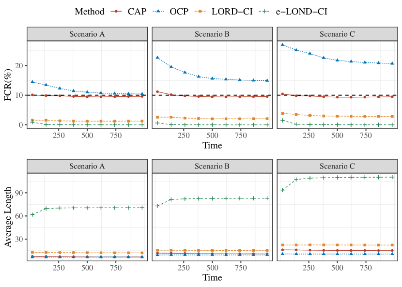
Figure F.1: Real-time FCR plot and average length plot from time $20$ to $2,000$ for e-LOND-CI. The selection rule is Dec-driven and the incremental holdout set with window size $200$ is considered. The black dashed line represents the target FCR level $10\%$.

We provide additional simulations for e-LOND-CI. Figure F.1 illustrates the FCR and average length under different scenarios using decision-driven selection for e-LOND-CI. As it is shown, the prediction intervals produced by e-LOND-CI are considerably wide, limiting the e-LOND-CI to provide non-trivial uncertainty quantification.

F.2 Details of online multiple testing procedure using conformal $p$-values

Recall that the selection problem can be viewed as the following multiple hypothesis tests: for time $t$ and some constant $b_{0}\in{\mathbb{R}}$,

$$H_{0,t}:Y_{i}\geq b_{0}\quad\text{v.s.}\quad H_{1,t}:Y_{t}<b_{0}.$$

Denote the additional labelled data set for computing conformal $p$-values as ${\mathcal{C}}_{p}$. We write the index set of null samples in ${\mathcal{C}}_{p}$ as ${\mathcal{C}}_{p,0}=\{i\in{\mathcal{C}}_{p}:Y_{i}\geq b_{0}\}$. For each test data point, the conformal $p$-value based on same-class calibration [Bates et al., 2023] can be calculated by

$$p_{t}=\frac{1+|\{i\in{\mathcal{C}}_{p,0}:g(X_{i})\leq g(X_{t})\}|}{|{\mathcal{C}}_{p,0}|+1},$$ (F.1)

where $g(x)=\hat{\mu}(x)-b_{0}$ is the nonconformity score function for constructing $p$-values.

To control the $\operatorname{FDR}$ at the level $\beta\in(0,1)$, we deploy the SAFFRON [Ramdas et al., 2018] procedure. The main idea of SAFFRON is to make a more precise estimation of current FDP by incorporating the null proportion information. Given $\beta\in(0,1)$, the user starts to pick a constant $\lambda\in(0,1)$ used for estimating the null proportion, an initial wealth $W_{0}\leq\beta$ and a positive non-increasing sequence $\{\gamma_{j}\}_{j=1}^{\infty}$ of summing to one. The SAFFRON begins by allocation the rejection threshold $\beta_{1}=\min\{(1-\lambda)\gamma_{1}W_{0},\lambda\}$ and for $t\leq 2$ it sets:

$$\beta_{t}=\min\Big{\{}\lambda,(1-\lambda)\Big{(}W_{0}\gamma_{t-C_{0+}}+(\alpha-W_{0})\gamma_{t-\tau_{1}-C_{1+}}+\sum_{j\geq 2}\beta\gamma_{t-\tau_{j}-C_{j+}}\Big{)}\Big{\}},$$

where $\tau_{j}$ is the time of the $j$-th rejection (define $\tau_{0}=0$), and $C_{j+}=\sum_{i=\tau_{j}+1}^{t-1}\mathds{1}\{p_{i}\leq\lambda\}$. Thus for each time $t$, we reject the hypothesis if $p_{t}\leq\beta_{t}$. In our experiment, we set defaulted parameters, where $W_{0}=\beta/2$, $\lambda=0.5$ and $\gamma_{j}\propto 1/j^{1.6}$.

F.3 Experiments on fixed calibration set

We verify the validity of our algorithms with respect to a fixed calibration set. The size of the fixed calibration set is set as $50$, and the procedure stops at time $1,000$. We design a decision-driven selection strategy. At each time $t$, the selection indicator is $S_{t}=\mathds{1}\{V_{t}>\tau({\mathbf{S}}(t))\}$, where $V_{t}=\widehat{\mu}(X_{t})$ and $\tau(s)=\tau_{0}-\min\{s/50,2\}$. The parameter $\tau_{0}$ is pre-fixed for each scenario. Three different initial thresholds for different scenarios due to the change of the scale of the data. The thresholds $\tau_{0}$ are set as $1$, $4$ and $3$ for Scenarios A, B and C respectively. This selection rule is more aggressive when the number of selected samples is small.

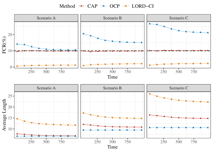
Figure F.2: Real-time FCR plot and average length plot from time $20$ to $1,000$ for fixed calibration set after $500$ replications. The black dashed line represents the target FCR level $10\%$.

We choose the target FCR level as $\alpha=10\%$. The real-time results are demonstrated in Figure F.2 based on $500$ times repetitions. Across all the settings, it is evident that the SCOP is able to deliver quite accurate FCR control and have more narrowed PIs.

F.4 Impacts of initial holdout set size

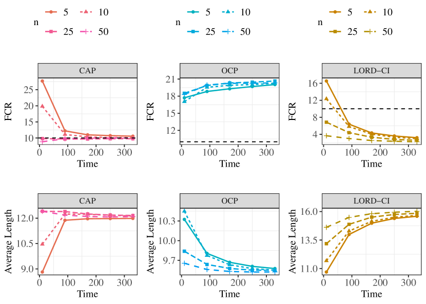
Figure F.3: Real-time FCR and average length from time $20$ to $400$ using different sizes of the initial holdout set for CAP, OCP and LORD-CI. The basic setting is Scenario B and the quantile selection rule is used. The black dashed line denotes the target FCR level $10\%$.

Next we assess the impact of the initial holdout set size $n$. For simplicity, we focus on Scenario B and employ the quantile selection rule. We vary the initial size $n$ within the set $\{5,10,25,50\}$, and summarize the results among $500$ repetitions in Figure F.3. When the initial size is small, the CAP tends to exhibit overconfidence at the start of the stage. However, as time progresses, the FCR level approaches the target of $10\%$. Conversely, with a moderate initial size such as $25$, the CAP achieves tight FCR control throughout the procedure, thereby confirming our theoretical guarantee. A similar phenomenon is also observed with OCP and LORD-CI, wherein the FCR at the initial stage significantly diverges from the FCR at the end stage when a small value of $n$ is utilized. To ensure a stabilized FCR control throughout the entire procedure, we recommend employing a moderate size of for the initial holdout set.

F.5 Comparisons of $\widehat{{\mathcal{C}}}_{t}^{\rm{inter}}$ and $\widehat{{\mathcal{C}}}_{t}^{\rm{naive}}$ for decision-driven selection rule

We make empirical comparisons of $\widehat{{\mathcal{C}}}_{t}^{\rm{inter}}$ and $\widehat{{\mathcal{C}}}_{t}^{\rm{naive}}$ using the same Dec-driven rule over incremental holdout set. All the settings are the same except for that we use an initial holdout set with size $20$. The results are demonstrated in Figure F.4. The CAP-inter ($\widehat{{\mathcal{C}}}_{t}^{\rm{inter}}$) has smaller FCR value and a slightly wider interval compared to CAP-naive ($\widehat{{\mathcal{C}}}_{t}^{\rm{naive}}$). But the difference is not significant and the power loss is acceptable.

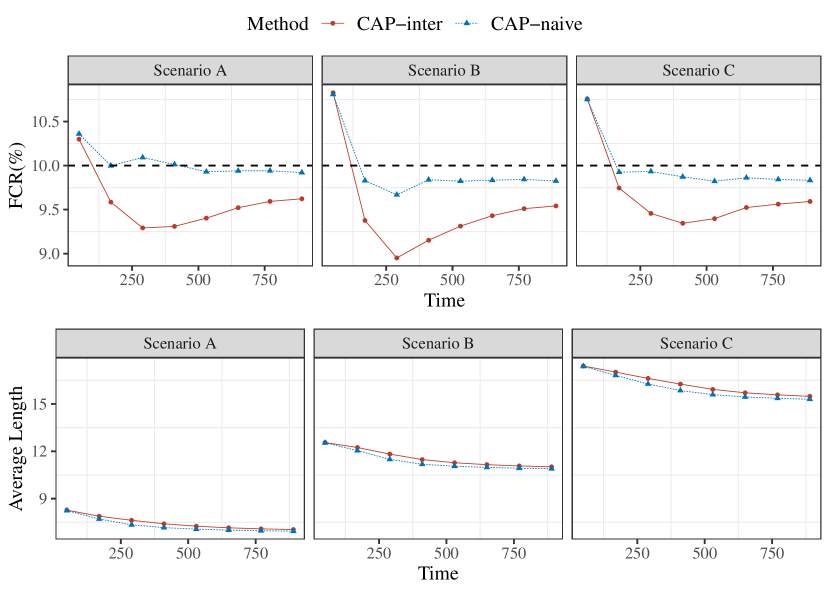
Figure F.4: Comparison for CAP-inter and CAP-naive by real-time FCR plot and average length plot from time $50$ to $1000$ after $500$ replications. The black dashed line represents the target FCR level $10\%$.

F.6 Comparisons of $\widehat{{\mathcal{C}}}_{t}^{\rm{swap}}$ and $\widehat{{\mathcal{C}}}_{t}^{\rm{naive}}$ for symmetric selection rule

We study the difference of $\widehat{{\mathcal{C}}}_{t}^{\rm{swap}}$ and $\widehat{{\mathcal{C}}}_{t}^{\rm{naive}}$ for quantile selection rule. Figure F.5 displays the results for both methods under three scenarios using $70\%$-quantile selection rule. The CAP-Swap (using $\widehat{{\mathcal{C}}}_{t}^{\rm{swap}}$) and CAP-naive (using $\widehat{{\mathcal{C}}}_{t}^{\rm{naive}}$) perform almost identical.

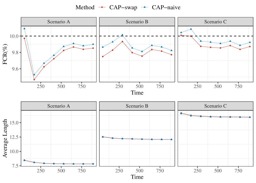
Figure F.5: Comparison for CAP-swap and CAP-naive by real-time FCR plot and average length plot from time $50$ to $1,000$ for full calibration set after $500$ replications. The black dashed line represents the target FCR level $10\%$.

F.7 Additional real-data application to airfoil self-noise

Airflow-induced noise prediction and reduction is one of the priorities for both the energy and aviation industries [Brooks et al., 1989]. We consider applying our method to the airfoil data set from the UCI Machine Learning Repository [Dua and Graff, 2017], which involves $1,503$ observations of a response $Y$ (scaled sound pressure level of NASA airfoils), and a five-dimensional feature including log frequency, angle of attack, chord length, free-stream velocity, and suction side log displacement thickness. The data is obtained via a series of aerodynamic and acoustic tests, and the distributions of the data are in different patterns at different times. This dataset can be regarded as having distribution shifting over time, and we aim to implement the CAP-DtACI with the same parameters in Section 5.2 to solve this problem.

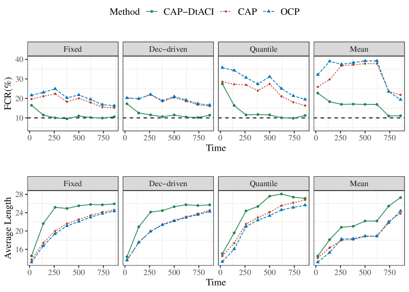
Figure F.6: Real-time FCR and average length from time $20$ to $900$ by $20$ replications for four selection rules in airfoil noise task. The black dashed line denotes the target FCR level $10\%$.

We reserve the first $480$ samples as a training set to train an SVM model with defaulted parameters, and then we use the following $23$ samples as the initial holdout set. Since the data is in time order, we take an integrated period of size 900 from the remaining samples as the online data set. We treat each choice of the periods (starting at different times) as a repetition to compute the FCR and average length. Four selection rules are considered here: fixed selection rule with $S_{t}=\mathds{1}\{\widehat{\mu}(X_{t})>115\}$; decision-driven selection rule with $S_{t}=\mathds{1}\{\widehat{\mu}(X_{t})>110+\min\{\sum_{j=0}^{t-1}S_{j}/30,10\}\}$; quantile selection rule with $S_{t}=\mathds{1}\{\widehat{\mu}(X_{t})>\mathcal{A}(\{\widehat{\mu}(X_{i})\}_{i=t-500}^{t-1})\}$ where $\mathcal{A}(\{\widehat{\mu}(X_{i})\}_{i=t-500}^{t-1})$ is the $35\%$-quantile of $\{\widehat{\mu}(X_{i})\}_{i=t-500}^{t-1}$; mean selection rule with $S_{t}=\mathds{1}\{\widehat{\mu}(X_{t})>\sum_{i=t-500}^{t-1}\widehat{\mu}(X_{i})/500\}$. We adopt a windowed scheme with window size $500$, and set the target FCR level $\alpha=10\%$.

Figure F.6 summarizes the FCR and average lengths of CAP-DtACI, CAP and OCP among 20 replications. As illustrated, the CAP-DtACI performs well in delivering FCR close to the target level as time grows across almost every setting. In contrast, CAP and OCP cannot obtain the desired FCR control due to a lack of consideration of distribution shifts.

References

- Aharoni and Rosset [2014] Ehud Aharoni and Saharon Rosset. Generalized -investing: definitions, optimality results and application to public databases. Journal of the Royal Statistical Society: Series B (Statistical Methodology), pages 771–794, 2014.
- Angelopoulos and Bates [2021] Anastasios N Angelopoulos and Stephen Bates. A gentle introduction to conformal prediction and distribution-free uncertainty quantification. arXiv preprint arXiv:2107.07511, 2021.
- Bao et al. [2024] Yajie Bao, Yuyang Huo, Haojie Ren, and Changliang Zou. Selective conformal inference with false coverage-statement rate control. Biometrika, page asae010, 02 2024. ISSN 1464-3510. doi: 10.1093/biomet/asae010. URL https://doi.org/10.1093/biomet/asae010.
- Barber et al. [2021] Rina Foygel Barber, Emmanuel J Candès, Aaditya Ramdas, and Ryan J Tibshirani. Predictive inference with the jackknife+. The Annals of Statistics, 49(1):486–507, 2021.
- Barber et al. [2023] Rina Foygel Barber, Emmanuel J Candès, Aaditya Ramdas, and Ryan J Tibshirani. Conformal prediction beyond exchangeability. The Annals of Statistics, 51(2):816–845, 2023.
- Bates et al. [2023] Stephen Bates, Emmanuel Candès, Lihua Lei, Yaniv Romano, and Matteo Sesia. Testing for outliers with conformal p-values. The Annals of Statistics, 51(1):149–178, 2023.
- Benjamini and Yekutieli [2005] Yoav Benjamini and Daniel Yekutieli. False discovery rate–adjusted multiple confidence intervals for selected parameters. Journal of the American Statistical Association, 100(469):71–81, 2005.
- Bollerslev [1986] Tim Bollerslev. Generalized autoregressive conditional heteroskedasticity. Journal of econometrics, 31(3):307–327, 1986.
- Brooks et al. [1989] Thomas F Brooks, D Stuart Pope, and Michael A Marcolini. Airfoil self-noise and prediction. Technical report, 1989.
- Chernozhukov et al. [2021] Victor Chernozhukov, Kaspar Wüthrich, and Yinchu Zhu. An exact and robust conformal inference method for counterfactual and synthetic controls. Journal of the American Statistical Association, 116(536):1849–1864, 2021.
- Davis et al. [2011] Mindy I Davis, Jeremy P Hunt, Sanna Herrgard, Pietro Ciceri, Lisa M Wodicka, Gabriel Pallares, Michael Hocker, Daniel K Treiber, and Patrick P Zarrinkar. Comprehensive analysis of kinase inhibitor selectivity. Nature Biotechnology, 29(11):1046–1051, 2011.
- Dua and Graff [2017] Dheeru Dua and Casey Graff. UCI machine learning repository, 2017. URL http://archive.ics.uci.edu/ml.
- Dwork et al. [2006] Cynthia Dwork, Frank McSherry, Kobbi Nissim, and Adam Smith. Calibrating noise to sensitivity in private data analysis. In Theory of Cryptography: Third Theory of Cryptography Conference, TCC 2006, New York, NY, USA, March 4-7, 2006. Proceedings 3, pages 265–284. Springer, 2006.
- Fithian et al. [2014] William Fithian, Dennis Sun, and Jonathan Taylor. Optimal inference after model selection. arXiv preprint arXiv:1410.2597, 2014.
- Foster and Stine [2008] Dean P Foster and Robert A Stine. -investing: a procedure for sequential control of expected false discoveries. Journal of the Royal Statistical Society: Series B (Statistical Methodology), 70(2):429–444, 2008.
- Foygel Barber et al. [2021] Rina Foygel Barber, Emmanuel J Candès, Aaditya Ramdas, and Ryan J Tibshirani. The limits of distribution-free conditional predictive inference. Information and Inference, 10(2):455–482, 2021. doi: 10.1093/imaiai/iaaa017.
- Gibbs and Candès [2021] Isaac Gibbs and Emmanuel Candès. Adaptive conformal inference under distribution shift. Advances in Neural Information Processing Systems, 34:1660–1672, 2021.
- Gibbs and Candès [2022] Isaac Gibbs and Emmanuel Candès. Conformal inference for online prediction with arbitrary distribution shifts. arXiv preprint arXiv:2208.08401, 2022.
- Gradu et al. [2023] Paula Gradu, Elad Hazan, and Edgar Minasyan. Adaptive regret for control of time-varying dynamics. In Learning for Dynamics and Control Conference, pages 560–572. PMLR, 2023.
- Huang et al. [2020] Kexin Huang, Tianfan Fu, Lucas M Glass, Marinka Zitnik, Cao Xiao, and Jimeng Sun. Deeppurpose: a deep learning library for drug–target interaction prediction. Bioinformatics, 36(22-23):5545–5547, 2020.
- Huang et al. [2022] Kexin Huang, Tianfan Fu, Wenhao Gao, Yue Zhao, Yusuf Roohani, Jure Leskovec, Connor W Coley, Cao Xiao, Jimeng Sun, and Marinka Zitnik. Artificial intelligence foundation for therapeutic science. Nature Chemical Biology, 18(10):1033–1036, 2022.
- Javanmard and Montanari [2015] Adel Javanmard and Andrea Montanari. On online control of false discovery rate. arXiv preprint arXiv:1502.06197, 2015.
- Javanmard and Montanari [2018] Adel Javanmard and Andrea Montanari. Online rules for control of false discovery rate and false discovery exceedance. The Annals of statistics, 46(2):526–554, 2018.
- Jin and Candès [2023a] Ying Jin and Emmanuel J Candès. Selection by prediction with conformal p-values. Journal of Machine Learning Research, 24(244):1–41, 2023a.
- Jin and Candès [2023b] Ying Jin and Emmanuel J Candès. Model-free selective inference under covariate shift via weighted conformal p-values. arXiv preprint arXiv:2307.09291, 2023b.
- Lee et al. [2016] Jason D Lee, Dennis L Sun, Yuekai Sun, and Jonathan E Taylor. Exact post-selection inference, with application to the lasso. The Annals of Statistics, 44(3):907–927, 2016.
- Lei and Wasserman [2014] Jing Lei and Larry Wasserman. Distribution-free prediction bands for non-parametric regression. Journal of the Royal Statistical Society: Series B (Statistical Methodology), 76(1):71–96, 2014.
- Lei et al. [2018] Jing Lei, Max G’Sell, Alessandro Rinaldo, Ryan J Tibshirani, and Larry Wasserman. Distribution-free predictive inference for regression. Journal of the American Statistical Association, 113(523):1094–1111, 2018.
- Papadopoulos et al. [2002] Harris Papadopoulos, Kostas Proedrou, Volodya Vovk, and Alex Gammerman. Inductive confidence machines for regression. In European Conference on Machine Learning, pages 345–356. New York: Springer, 2002.
- Ramdas et al. [2017] Aaditya Ramdas, Fanny Yang, Martin J Wainwright, and Michael I Jordan. Online control of the false discovery rate with decaying memory. Advances in Neural Information Processing Systems, 30:5655–5664, 2017.
- Ramdas et al. [2018] Aaditya Ramdas, Tijana Zrnic, Martin Wainwright, and Michael Jordan. Saffron: an adaptive algorithm for online control of the false discovery rate. In International Conference on Machine Learning, pages 4286–4294. PMLR, 2018.
- Romano et al. [2019] Yaniv Romano, Evan Patterson, and Emmanuel Candès. Conformalized quantile regression. Advances in Neural Information Processing Systems, 32:3543–3553, 2019.
- Sadinle et al. [2019] Mauricio Sadinle, Jing Lei, and Larry Wasserman. Least ambiguous set-valued classifiers with bounded error levels. Journal of the American Statistical Association, 114(525):223–234, 2019.
- Shafer and Vovk [2008] Glenn Shafer and Vladimir Vovk. A tutorial on conformal prediction. Journal of Machine Learning Research, 9(3):371–421, 2008.
- Taylor and Tibshirani [2018] Jonathan Taylor and Robert Tibshirani. Post-selection inference for-penalized likelihood models. Canadian Journal of Statistics, 46(1):41–61, 2018.
- Tibshirani et al. [2019] Ryan J Tibshirani, Rina Foygel Barber, Emmanuel Candès, and Aaditya Ramdas. Conformal prediction under covariate shift. Advances in Neural Information Processing Systems, 32:2530–2540, 2019.
- Vovk [1990] Vladimir Vovk. Aggregating strategies. In Proceedings of 3rd Annu. Workshop on Comput. Learning Theory, pages 371–383, 1990.
- Vovk and Wang [2021] Vladimir Vovk and Ruodu Wang. E-values: Calibration, combination and applications. The Annals of Statistics, 49(3):1736–1754, 2021.
- Vovk et al. [2005] Vladimir Vovk, Alexander Gammerman, and Glenn Shafer. Algorithmic learning in a random world. Springer Science & Business Media, 2005.
- Vovk et al. [1999] Volodya Vovk, Alexander Gammerman, and Craig Saunders. Machine-learning applications of algorithmic randomness. In International Conference on Machine Learning, pages 444–453, 1999.
- Weinstein and Ramdas [2020] Asaf Weinstein and Aaditya Ramdas. Online control of the false coverage rate and false sign rate. In International Conference on Machine Learning, pages 10193–10202, 2020.
- Weinstein et al. [2013] Asaf Weinstein, William Fithian, and Yoav Benjamini. Selection adjusted confidence intervals with more power to determine the sign. Journal of the American Statistical Association, 108(501):165–176, 2013.
- Wintenberger [2017] Olivier Wintenberger. Optimal learning with bernstein online aggregation. Machine Learning, 106:119–141, 2017.
- Xu and Ramdas [2023] Ziyu Xu and Aaditya Ramdas. Online multiple testing with e-values. arXiv preprint arXiv:2311.06412, 2023.
- Xu et al. [2022] Ziyu Xu, Ruodu Wang, and Aaditya Ramdas. Post-selection inference for e-value based confidence intervals. arXiv preprint arXiv:2203.12572, 2022.
- Zhao [2022] Haibing Zhao. General ways to improve false coverage rate-adjusted selective confidence intervals. Biometrika, 109(1):153–164, 2022.