Abstract

We studied the one-loop prediction for the single production of a Higgs-like boson in association with a photon in electron-positron collisions in the context of two Higgs doublet type-II seesaw model (2HDMcT). We explored to what extent the new scalars in the (2HDMcT) spectrum affect its production cross-section, the ratio $R_{\gamma h_{1}}$ as well as the signal strengths $R_{\gamma Z}$ and $R_{\gamma\gamma}$ when $h_{1}$ is identified with the observed $SM$ Higgs boson within the $2HDMcT$ delimited parameter space. More specifically, we focused on $e^{+}e^{-}\to h_{1}\gamma$ process at one-loop, and analyzed how it evolves under a full set of theoretical constraints and the available experimental data, including $B\to X_{s}\gamma$ constraint at 95$\%$ C.L. Our analysis showed that these observables are particularly sensitive to the parameters $\alpha_{1}$, $\lambda_{7}$, $\lambda_{9}$, the trilinear Higgs couplings and to the charged Higgs masses. We found that $\sigma(e^{+}e^{-}\to h_{1}\gamma)$ can significantly be enhanced up to $8.1\,\,10^{-2}$ fb, so exceeding the Standard Model prediction. Additionally, as a byproduct, we also found that $R_{\gamma h_{1}}$ is entirely correlated with both the $h_{1}\to\gamma\gamma$ and $h_{1}\to\gamma Z$ signal strengths.

1 Introduction

The discovery of the Higgs boson, the last missing piece in the completion of the Standard Model ($SM$), by the ATLAS [1] and CMS [2] collaborations provided an experimental evidence for the Brout-Englert-Higgs mechanism. Since then, major ongoing studies have focused on exploring in detail the properties of the Higgs boson with the aim to enhance our understanding of the fundamental laws of nature. Although most of the $SM$’s predictions have been tested successfully to a high level of accuracy[3, 4, 5], it still suffers from drawbacks since it failed to explain several established physical phenomena. As examples, the problem of dark matter[6, 7], the hierarchy problem [8], and the neutrino mass generation [9, 10] do not fit in the SM.

To address these issues, a plethora of new physics models have been proposed in literature. Among these beyond the Standard Model ($BSM$), scenarios relying on an extended Higgs sectors with new scalar fields, as the popular two Higgs Doublet Model (2HDM) [11, 12, 13, 14, 15, 16], the Higgs Triplet Models (HTM) [16, 14] and recently 2HDM augmented by a complex triplet scalar, dubbed the two Higgs Doublet Type-II Seesaw model (2HDMcT) [17, 18]. Since the spectra of these models generally predict additional Higgs bosons with novel features, searching for these new scalars has been actively conducted as a key focus and one of the major motivations for the current and future experiments, especially at LHC [19, 20, 21, 22, 23, 24, 25]. Besides, as no direct evidence for new physics has been seen yet, precision measurements of the Higgs boson properties and couplings [26, 27, 28, 29, 30] to other new scalars can offer a promising opportunity for a potential discovery of new physics. Indeed, more accurate understanding of the Higgs boson and the measurements of its couplings with high levels of precision is the main goal of future $e^{+}e^{-}$ colliders [31] such as the International Linear Collider (ILC) [32, 33], Compact Linear Collider (CLIC) [34, 31], Circular Electron-Positron Collider (CEPC) [35, 36, 37], and Future Circular Collider (FCC) [38, 39]. Compared to hadron colliders, these colliders, featuring a cleaner $e^{+}e^{-}$ background, can yield substantial improvements over LHC measurements [40].

The associated production of Standard Model (SM) Higgs boson with a photon, $e^{+}e^{-}\to h_{1}\gamma$, is well suited to study the Higgs-gauge bosons couplings such as the $h_{1}\gamma\gamma$ and $h_{1}\gamma Z$ couplings. Since the production rate can be sizably amplified in the presence of new physics contributions as compared to the Standard Model, this process may serve as a potential discovery channel. This process was investigated in the (SM) [41, 42, 43] and recently in some $BSM$ scenarios as the inert Higgs doublet model [44], (HTM) [45], the minimal supersymmetric standard model (MSSM) [46, 47] and the effective field theory [48].

In this work, we investigate the single production of the neutral Higgs boson in association with a photon in the electron positron collisions within the Two Higgs Doublet Type II seesaw Model 2HDMcT. To do that, we implement a full set of theoretical constraints originated from perturbative unitarity, electroweak vacuum stability, as well as the experimental Higgs exclusion limits from LEP, LHC and Tevatron. Since the mass generation from seesaw mechanism is similar to the Brout-Englert-Higgs mechanism, 2HDMcT model is appealing, displaying many phenomenological features especially different from those emerging in 2HDM scalar sector. Apart its broader spectrum than 2HDM’s one, the doubly charged Higgs $H^{++}$, as a smoking gun of 2HDMcT, $H^{++}$ is currently intensively searched for at ATLAS and CMS, by means of promising decay channels, such as $H^{++}H^{--}$ and $H_{i}^{+}H_{i}^{-}$ $(i=1,2)$, decaying to the same sign di-lepton [17]. Additionally, beyond Higgs phenomenology, it has been demonstrated that interactions between doublet and triplet fields may induce a strong first order electroweak phase transition, which provide conditions for the generation of the baryon asymmetry through electroweak baryongenesis [49].

This paper is organized as follows: In Sect.2, we briefly review 2HDMcT model and mention some theoretical and experimental constraints imposed on the model. In Sect.3 we study the two processes $e^{+}e^{-}\to h_{1}\gamma$ and $e^{-}\gamma\to h_{1}e^{-}$ in 2HDMcT and discuss the correlation of the signal strengths for the one loop induced processes $h_{1}\to\gamma\gamma$ and $h_{1}\to Z\gamma$ in 2HDMcT. Sect.4 is devoted to our conclusion.

2 Two Higgs doublet type-II seesaw model: Brief overview

The two Higgs doublet type II seesaw model has recently gained interest as a well-motivated extension of the 2HDM. Besides the two Higgs doublets with hypercharge $Y=+1$, 2HDM is augmented with one colorless triplet field $\Delta$ transforming under the $SU(2)_{L}$ gauge group as a complex scalar with $Y_{\Delta}=2$.

$$\Phi_{1}=\left(\begin{array}[]{c}\phi_{1}^{+}\\ \phi_{1}^{0}\\ \end{array}\right)\quad{\rm,}\quad\Phi_{2}=\left(\begin{array}[]{c}\phi_{2}^{+}\\ \phi_{2}^{0}\\ \end{array}\right)\quad{\rm and}\quad\begin{matrix}\Delta&=&\left(\begin{array}[]{cc}\delta^{+}/\sqrt{2}&\delta^{++}\\ (v_{t}+\delta^{0}+i\eta_{0})/\sqrt{2}&-\delta^{+}/\sqrt{2}\\ \end{array}\right)\end{matrix}$$ (1)

with $\phi_{1}^{0}=(v_{1}+\psi_{1}+i\eta_{1})/\sqrt{2}$, $\phi_{2}^{0}=(v_{2}+\psi_{2}+i\eta_{2})/\sqrt{2}$. $v_{1}$, $v_{2}$ and $v_{t}$ denote the vacuum expectation values of the Higgs doublets and triplet fields respectively, acquired when the electroweak symmetry is spontaneously broken, with $\sqrt{v_{1}^{2}+v_{2}^{2}+2v_{t}^{2}}=246$ GeV. Consequently, eleven physical Higgs states occur in the model spectrum: three CP-even neutral Higgs bosons $(h_{1},h_{2},h_{3})$, four simply charged Higgs bosons $(H_{1}^{\pm},H_{2}^{\pm})$, two CP odd Higgs $(A_{1},A_{2})$, and finally two doubly charged Higgs bosons $H^{\pm\pm}$. For details see Ref.[17].

The most general $SU(2)_{L}\times U(1)_{Y}$ invariant scalar potential in this model reads : [13, 17]:

$$V(\Phi_{1},\Phi_{2},\Delta) = m_{11}^{2}\Phi_{1}^{\dagger}\Phi_{1}+m_{22}^{2}\Phi_{2}^{\dagger}\Phi_{2}-[m_{12}^{2}\Phi_{1}^{\dagger}\Phi_{2}+{\rm h.c.}]+\frac{\lambda_{1}}{2}(\Phi_{1}^{\dagger}\Phi_{1})^{2}+\frac{\lambda_{2}}{2}(\Phi_{2}^{\dagger}\Phi_{2})^{2}$$ (2)

$$+ \lambda_{4}(\Phi_{1}^{\dagger}\Phi_{2})(\Phi_{2}^{\dagger}\Phi_{1})+\left\{\frac{\lambda_{5}}{2}(\Phi_{1}^{\dagger}\Phi_{2})^{2}+\big{[}\beta_{1}(\Phi_{1}^{\dagger}\Phi_{1})+\beta_{2}(\Phi_{2}^{\dagger}\Phi_{2})\big{]}\Phi_{1}^{\dagger}\Phi_{2}+{\rm h.c.}\right\}$$

$$+ \lambda_{3}(\Phi_{1}^{\dagger}\Phi_{1})(\Phi_{2}^{\dagger}\Phi_{2})+\lambda_{6}\,\Phi_{1}^{\dagger}\Phi_{1}Tr\Delta^{\dagger}{\Delta}+\lambda_{7}\,\Phi_{2}^{\dagger}\Phi_{2}Tr\Delta^{\dagger}{\Delta}$$

$$+ \left\{\mu_{1}\Phi_{1}^{T}{i}\sigma^{2}\Delta^{\dagger}\Phi_{1}+\mu_{2}\Phi_{2}^{T}{i}\sigma^{2}\Delta^{\dagger}\Phi_{2}+\mu_{3}\Phi_{1}^{T}{i}\sigma^{2}\Delta^{\dagger}\Phi_{2}+{\rm h.c.}\right\}+\lambda_{8}\,\Phi_{1}^{\dagger}{\Delta}\Delta^{\dagger}\Phi_{1}$$

$$+ \lambda_{9}\,\Phi_{2}^{\dagger}{\Delta}\Delta^{\dagger}\Phi_{2}+m^{2}_{\Delta}\,Tr(\Delta^{\dagger}{\Delta})+\bar{\lambda}_{8}(Tr\Delta^{\dagger}{\Delta})^{2}+\bar{\lambda}_{9}Tr(\Delta^{\dagger}{\Delta})^{2}$$

In this work we assume that $m_{11}^{2}$, $m_{22}^{2}$, $m_{\Delta}^{2}$, $m_{12}^{2}$, $\lambda_{1,2,3,4,5,6,7,8,9}$, $\bar{\lambda}_{8,9}$, $\mu_{1,2,3}$, $\beta_{1,2}$ are real parameters. To avoid Higgs mediated $FCNC_{s}$ at tree level, we consider $Z_{2}$ symmetry where $\beta_{1}=\beta_{2}=0$. Also the $Z_{2}$ symmetry is softly broken by the bi-linear terms proportional to $m_{12}^{2}$, $\mu_{1}$, $\mu_{2}$ and $\mu_{3}$ parameters. Thanks to the combination $v^{2}=v_{1}^{2}+v_{2}^{2}+2v_{t}^{2}=(2\sqrt{2}G_{F})^{-1}$ and the three minimization conditions, the scalar potential Eq. (2) has seventeen independent parameters, one choice is :

$\alpha_{1}$, $\alpha_{2}$, $\alpha_{3}$, $m_{h_{1}}$, $m_{h_{2}}$, $m_{h_{3}}$, $m_{H^{\pm\pm}}$, $\lambda_{1}$, $\lambda_{3}$, $\lambda_{4}$, $\lambda_{6}$, $\lambda_{8}$, $\bar{\lambda}_{8}$, $\bar{\lambda}_{9}$, $\mu_{1}$, $v_{t}$ and $\tan\beta$

where $\alpha_{i=1,2,3}$ are the CP-even mixing angles and $\tan\beta=v_{2}/v_{1}$.

In our subsequent analysis $h_{1}$ is identified to the SM-like Higgs boson with $m_{h}=125$ GeV [1, 2], so the scalar potential is described by sixteen free parameters. $\mathcal{L}_{\rm Yukawa}$ contains all the Yukawa sector of the Two Higgs Doublet Model plus one extra Yukawa term emerging from the triplet field and generating, after spontaneous symmetry breaking, a small Majorana mass terms for the neutrinos.

$$-\mathcal{L}_{\rm Yukawa}\supset-Y_{\nu}L^{T}C\otimes i\sigma^{2}\Delta L+{\rm h.c.}$$ (3)

For the type II (2HDMcT-II), up quarks interact with $\Phi_{2}$, while leptons and down quarks with $\Phi_{1}$ as :

$$-{\cal L}^{II}_{Yukawa} = -y_{u}\bar{Q}_{L}\tilde{\Phi}_{2}u_{R}-y_{d}\bar{Q}_{L}\Phi_{1}d_{R}-y_{\ell}\bar{L}_{L}\Phi_{1}\ell_{R}+h.c\,,$$ (4)

Here $Q_{L}$ and $L_{L}$ represent the left-handed quark and lepton doublets, $u_{R}$, $d_{R}$, and $\ell_{R}$ are the right-handed up-type quark, down-type quark, and lepton singlets. $\Phi_{1}$ and $\Phi_{2}$ are the two Higgs doublets , with $\tilde{\Phi}_{2}=i\sigma_{2}\Phi_{2}^{*}$. $y_{u}$, $y_{d}$, and $y_{\ell}$ are the Yukawa couplings for the up, down-type quarks and leptons, respectively.

$\phi$	$\xi^{u}_{\phi}$	$\xi^{d}_{\phi}$	$\xi^{\ell}_{\phi}$
$h_{1}$	$\frac{\mathcal{E}_{12}}{s_{\beta}}$	$-\frac{\mathcal{E}_{11}}{c_{\beta}}$	$-\frac{\mathcal{E}_{11}}{c_{\beta}}$
$h_{2}$	$\frac{\mathcal{E}_{22}}{s_{\beta}}$	$-\frac{\mathcal{E}_{21}}{c_{\beta}}$	$-\frac{\mathcal{E}_{21}}{c_{\beta}}$
$h_{3}$	$\frac{\mathcal{E}_{32}}{s_{\beta}}$	$-\frac{\mathcal{E}_{31}}{c_{\beta}}$	$-\frac{\mathcal{E}_{31}}{c_{\beta}}$

Table 1: Yukawa couplings of the $h_{1}$, $h_{2}$, and $h_{3}$ bosons to the quarks and leptons in 2HDMcT-II

2.1 Theoretical and Experimental Constraints

The phenomenological analysis in 2HDMcT is performed via implementation of a full set of theoretical constraints  [17, 18] as well as the Higgs exclusion limits from various experimental measurements at colliders, namely :

• Unitarity : The scattering processes must obey the perturbative unitarity.

• Perturbativity: The quartic couplings of the scalar potential are constrained by the following conditions:$|\lambda_{i}|<8\pi$ for each $i=1,..,5$.

• Vacuum stability : Boundedness from below $BFB$ arising from the positivity in any direction of the fields $\Phi_{i}$, $\Delta$.

• Electroweak precision observables: The oblique parameters $S,T$ and $U$ [50, 51] have been calculated in $2HDMcT$ [18]. The analysis of the precision electroweak data in light of the new PDG mass of the $W$ boson yields [52]:

  $$S=0.05\pm 0.08,\ \ T=0.09\pm 0.07,\ \ \rho_{ST}=0.92,$$

• To further delimit the allowed parameter space, the HiggsTools package [53] is employed. This ensures that the allowed parameter regions align with the observed properties of the $125$ GeV Higgs boson ( HiggsSignals [54, 55, 56, 53]) and with the limits from searches for additional Higgs bosons at the LHC and at LEP ( HiggsBounds [57, 58, 59, 60, 53]).

• Flavour constraints: Flavour constraints are also implemented in our analysis. We used $B$-physics derived results derived in [18] as well as the experimental data at 2$\sigma$ [61] displayed in Table 2.

Observable	Experimental result	95% C.L.
BR($\bar{B}\to X_{s}\gamma$)[18]	$(3.49\pm 0.19)\times 10^{-4}$[61]	$[3.11\times 10^{-4},3.87\times 10^{-4}]$

Table 2: Experimental result of flavor observable: $\bar{B}\to X_{s}\gamma$ at 95$\%$ C.L.

3 $e^{+}e^{-}\to\gamma h_{1}$ and $e^{-}\gamma\to e^{-}h_{1}$ in 2HDMcT

3.1 Process topology

The $e^{+}e^{-}\to\gamma h_{1}$ process has been studied in many of beyond the Standard Model frameworks. In the 2HDMcT, at tree level, the associated production processes $e^{+}e^{-}\to\gamma h_{1}$ and $e^{-}\gamma\to e^{-}h_{1}$ are intermediated by the t-channel and s-channel electron exchange diagrams respectively. However, the former diagrams are suppressed by the electron mass. At one-loop these diagrams are mediated by the self-energy, box, and triangle diagrams and hence they are sensitive to all virtual particles inside the loop including the charged Higgs states, $H^{\pm}_{1}$, $H^{\pm}_{2}$ and $H^{\pm\pm}$, predicted by the model.

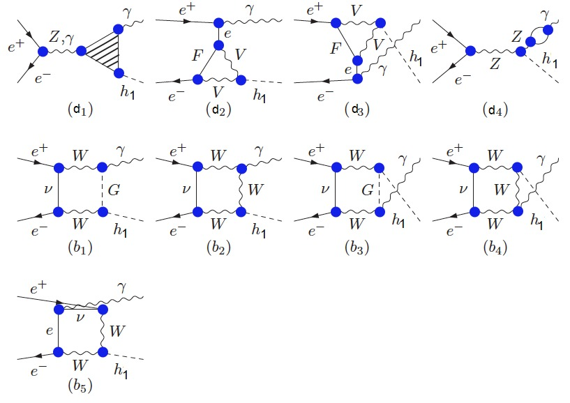
Figure 1: Feynman diagrams involving the charged contributions to $e^{-}\,e^{+}\,\,\to\,\,\gamma\,h_{1}$ process in 2HDMcT. In $d_{1}$ and $d_{4}$ diagrams, the loops receive contributions from all SM particles as well as the charged Higgs bosons $H^{\pm}_{1}$, $H^{\pm}_{2}$ and $H^{\pm\pm}$. Generic diagrams $d_{2},d_{3}$, depict $h_{1}\gamma V$, $V=\gamma,\;Z$.

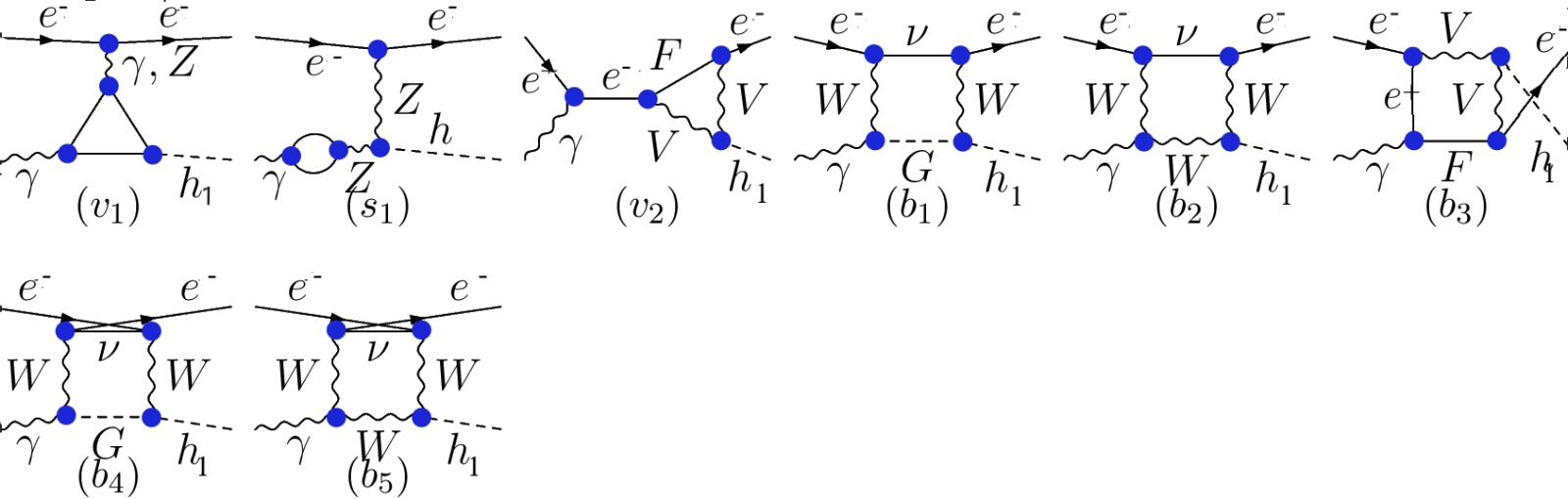
Figure 2: Feynman diagrams involving the charged contributions to $e^{-}\gamma\to e^{-}h_{1}$ process in the 2HDMcT. In diagrams $v_{1}$, we depict all possible charged particles. Diagrams $s_{1}$ receive contributions from all SM particles and from $H^{\pm}_{1}$, $H^{\pm}_{2}$ and $H^{\pm\pm}$ bosons.

Figs. 1, 2 and 3 illustrate the generic Feynman diagrams that effectively contribute to the $e^{+}e^{-}\to\gamma h_{1}$, $e^{-}\gamma\to e^{-}h_{1}$ and $h_{1}\to\gamma V$ processes, with $V=\gamma,\;Z$. Here $F$ stands for any fermionic particle, while $S$ denotes the charged states $H^{\pm}_{1}$, $H^{\pm}_{2}$ and $H^{\pm\pm}$.

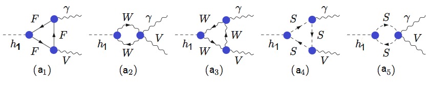
Figure 3: Feynman diagrams for the decay process $h_{1}\to\gamma V$ ($V=\gamma,\;Z$) in the 2HDMcT. $a_{4},a_{5}$ illustrate the contributions of $H^{\pm}_{1}$, $H^{\pm}_{2}$ and $H^{\pm\pm}$.

Our calculation is performed using dimensional regularization along with FeynArts and FormCalc packages [62, 63]. while the numerical evaluation of the scalar integrals is done with LoopTools [64, 65]. Note that the gauge invariance of our final results is assured once contributions from all box and triangle diagrams are summed. In the subsequent analysis, we introduce the ratio,

$$R_{\gamma h_{1}}\equiv\frac{\sigma(e^{+}e^{-}\to\gamma h_{1})}{\sigma_{\rm SM}(e^{+}e^{-}\to\gamma H)}$$ (5)

which is the total cross-sections in the $2HDMcT$ normalized to the SM one. Also we define the diphoton and $\gamma Z$ gauge bosons signal strengths, $R_{\gamma\gamma}$ and $R_{Z\gamma}$,

$$R_{\gamma\gamma(Z\gamma)}\equiv\frac{\sigma(gg\to h_{1})\times Br(h_{1}\to\gamma\gamma(Z\gamma))}{\sigma(gg\to H^{\rm SM})\times Br(H^{\rm SM}\to\gamma\gamma(Z\gamma))}$$ (6)

Compared with the Standard Model, the amplitudes for the loop processes $e^{-}\gamma\to e^{-}h_{1}$, $e^{+}e^{-}\to\gamma h_{1}$ and $h_{1}\to\gamma V$ ($V=\gamma,\;Z$) receive additional contributions from the $H^{\pm}_{1}$, $H^{\pm}_{2}$ and $H^{\pm\pm}$, the charged Higgs bosons predicted by the model spectrum. These amplitudes are essentially proportionals to the couplings with $h_{1}$ Higgs boson,

$$\bar{\lambda}_{h_{1}H^{\pm}_{1}H^{\pm}_{1}} = \frac{s_{w}}{2em_{w}}\left(2\mathcal{C}_{21}^{2}\left(\lambda_{6}\mathcal{E}_{13}v_{\Delta}+\lambda_{1}v_{1}\mathcal{E}_{11}+\lambda_{3}v_{2}\mathcal{E}_{12}\right)\right.$$ (7)

$$+2\mathcal{C}_{22}^{2}\left(\lambda_{7}\mathcal{E}_{13}v_{\Delta}+\lambda_{2}v_{2}\mathcal{E}_{12}+\lambda_{3}v_{1}\mathcal{E}_{11}\right)$$

$$+\mathcal{C}_{23}^{2}\left(2\mathcal{E}_{13}(2\overline{\lambda_{8}}+\overline{\lambda_{9}})v_{\Delta}+\left(2\lambda_{6}+\lambda_{8}\right)v_{1}\mathcal{E}_{11}+\left(2\lambda_{7}+\lambda_{9}\right)v_{2}\mathcal{E}_{12}\right)$$

$$+\mathcal{C}_{22}\mathcal{C}_{23}\left(\sqrt{2}\lambda_{9}\mathcal{E}_{12}v_{\Delta}+\sqrt{2}\lambda_{9}v_{2}\mathcal{E}_{13}-4\mu_{2}\mathcal{E}_{12}-2\mu_{3}\mathcal{E}_{11}\right)$$

$$+\mathcal{C}_{21}\left(\right.\mathcal{C}_{23}\left(\sqrt{2}\lambda_{8}\mathcal{E}_{11}v_{\Delta}+\sqrt{2}\lambda_{8}v_{1}\mathcal{E}_{13}-4\mu_{1}\mathcal{E}_{11}-2\mu_{3}\mathcal{E}_{12}\right)$$

$$\left.+2\mathcal{C}_{22}\left(\lambda_{4}+\lambda_{5}\right)\left(v_{2}\mathcal{E}_{11}+v_{1}\mathcal{E}_{12}\right)\left.\right)\right)$$

$$\bar{\lambda}_{h_{1}H^{\pm}_{2}H^{\pm}_{2}} = \frac{s_{w}}{2em_{w}}\left(2\mathcal{C}_{31}^{2}\left(\lambda_{6}\mathcal{E}_{13}v_{\Delta}+\lambda_{1}v_{1}\mathcal{E}_{11}+\lambda_{3}v_{2}\mathcal{E}_{12}\right)\right.$$ (8)

$$+2\mathcal{C}_{32}^{2}\left(\lambda_{7}\mathcal{E}_{13}v_{\Delta}+\lambda_{2}v_{2}\mathcal{E}_{12}+\lambda_{3}v_{1}\mathcal{E}_{11}\right)$$

$$+\mathcal{C}_{33}^{2}\left(2\mathcal{E}_{13}(2\overline{\lambda_{8}}+\overline{\lambda_{9}})v_{\Delta}+\left(2\lambda_{6}+\lambda_{8}\right)v_{1}\mathcal{E}_{11}+\left(2\lambda_{7}+\lambda_{9}\right)v_{2}\mathcal{E}_{12}\right)$$

$$+\mathcal{C}_{32}\mathcal{C}_{33}\left(\sqrt{2}\lambda_{9}\mathcal{E}_{12}v_{\Delta}+\sqrt{2}\lambda_{9}v_{2}\mathcal{E}_{13}-4\mu_{2}\mathcal{E}_{12}-2\mu_{3}\mathcal{E}_{11}\right)$$

$$+\mathcal{C}_{31}\left(\right.\mathcal{C}_{33}\left(\sqrt{2}\lambda_{8}\mathcal{E}_{11}v_{\Delta}+\sqrt{2}\lambda_{8}v_{1}\mathcal{E}_{13}-4\mu_{1}\mathcal{E}_{11}-2\mu_{3}\mathcal{E}_{12}\right)$$

$$\left.+2\mathcal{C}_{32}\left(\lambda_{4}+\lambda_{5}\right)\left(v_{2}\mathcal{E}_{11}+v_{1}\mathcal{E}_{12}\right)\left.\right)\right)$$

$$\bar{\lambda}_{h_{1}H^{\pm\pm}H^{\pm\pm}} = \frac{s_{w}}{em_{w}}\left(2\overline{\lambda_{8}}\mathcal{E}_{13}v_{\Delta}+\lambda_{6}v_{1}\mathcal{E}_{11}+\lambda_{7}v_{2}\mathcal{E}_{12}\right)$$ (9)

At this stage it is worth noticing that:

• These couplings are mostly fixed by $\alpha_{1}$, $\lambda_{3}$, $\lambda_{4}$, $\lambda_{7}$ and $\lambda_{9}$ parameters when $\tan\beta$ get relatively large values.

• Depending on their signs the charged Higgs contributions can either enhance or suppress the $e^{+}e^{-}\to\gamma h_{1}$ and $h_{1}\to\gamma V$ ($V=\gamma,\;Z$) rates.

3.2 Results and analysis

Given that $h_{1}$ is identified as the Higgs-like boson, observed at the LHC with $m_{h_{1}}=125$ GeV, we perform scans within the allowed parameter space by implementation of the theoretical and experimental constraints mentioned above.
The following set of input parameters is used in the subsequent numerical analysis :

$$\mathcal{P}_{I}=\left\{\alpha_{1},\alpha_{2},\alpha_{3},m_{h_{1}},m_{h_{2}},\lambda_{1},\lambda_{3},\lambda_{4},\lambda_{6},\lambda_{7},\lambda_{8},\lambda_{9},\bar{\lambda}_{8},\bar{\lambda}_{9},\mu_{1},v_{t},\tan\beta\right\}$$ (10)

$$\begin{matrix}m_{h_{1}}=125\,\,\text{GeV},\,\,\,m_{h_{1}}\leq m_{h_{2}}\leq m_{h_{3}}\leq 1\,\text{TeV},\,\,\,\par 80\,\,\text{GeV}\leq m_{H^{\pm}_{1}},m_{H^{\pm}_{2}},m_{H^{\pm\pm}}\leq 1\,\text{TeV},\,\,\\ -2\pi\leq\lambda_{1}\leq 2\pi,\,\,-2\pi\leq\lambda_{3,4}\leq 2\pi,\,\,\,\,\,-2\pi\leq\lambda_{6,7}\leq 2\pi,\,\,\,-2\pi\leq\lambda_{8,9}\leq 2\pi,\,\,-2\pi\leq\bar{\lambda}_{8,9}\leq 2\pi\\ -\pi/2\leq\alpha_{1}\leq\pi/2,\,\,\alpha_{2}\approx 0,\,\,\,\alpha_{3}\approx 0,\,\,\mu_{1}=v_{t}=1\,\,\text{GeV},\,\,\tan\beta=8\end{matrix}$$ (11)

From Eqs. (7), (8), and (9) one can readily see that the effect of $H_{1}^{\pm}$, $H_{2}^{\pm}$ virtual states on $h_{1}\gamma\gamma$ and $h_{1}\gamma Z$ couplings introduces a strong sensitivity to $\alpha_{1}$, $\lambda_{3}$, $\lambda_{4}$, $\lambda_{7}$ and $\lambda_{9}$ , while $H^{\pm\pm}$ leads to a noticeable dependence on $\alpha_{1}$, $\lambda_{7}$. Comparatively, dependence on the other model parameters is either mild or negligible.

In Fig. 4, we show the allowed ranges for $(\lambda_{7},\,\,\lambda_{9})$ as well as with the size of the trilinear couplings $\bar{\lambda}_{h_{1}H_{1}^{\pm}H_{1}^{\pm}}$, $\bar{\lambda}_{h_{1}H_{2}^{\pm}H_{2}^{\pm}}$ and $\bar{\lambda}_{h_{1}H^{\pm\pm}H^{\pm\pm}}$. All generated points passed the full set of constraints at $2\sigma$. The upper panel displays a significant dependence between the $(\lambda_{7},\,\,\lambda_{9})$ parameters and the charged Higgs boson masses; $m_{H^{\pm}_{1}}$ (left), $m_{H^{\pm}_{2}}$ (middle) and $m_{H^{\pm\pm}}$ (right). We can clearly see that the input ranges for $-2\pi<\lambda_{7}<2\pi$ and $-2\pi<\lambda_{9}<2\pi$ are strongly reduced to $0<\lambda_{7}<2\pi$ and $-5.25<\lambda_{9}<1.01$ essentially due to the combination the BFB conditions with the Higgs boson exclusion limits implemented in HiggsTools. Also, one can easily notice that the parameters $\lambda_{7}$ and $\lambda_{9}$ have opposite effects on the trilinear couplings, as illustrated by the middle and lower panels in Fig. 4: $\lambda_{7}$ increases $\bar{\lambda}_{h_{1}H^{\pm\pm}H^{\mp\mp}}$,$\bar{\lambda}_{h_{1}H_{1}^{\pm}H_{1}^{\pm}}$,$\bar{\lambda}_{h_{1}H_{2}^{\pm}H_{2}^{\pm}}$, while $\lambda_{9}$ weaken these trilinear couplings. Similarly compatibility with all the constraints oblige the parameters $\mu_{2,3}$ to undergo drastic reductions being confined within the mitigated intervals $0<\mu_{2}<8$ and $70<\mu_{3}<108$ respectively.

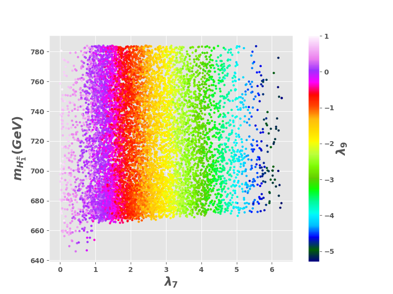
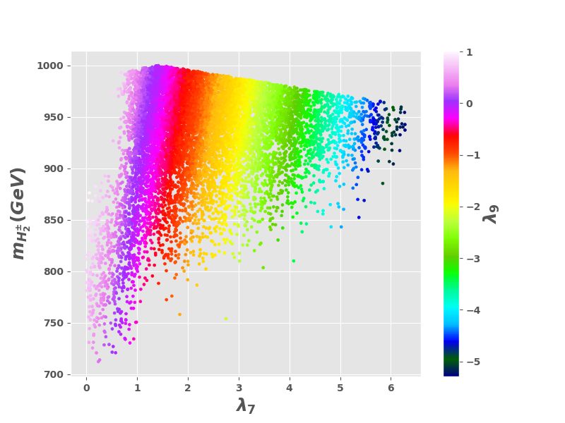
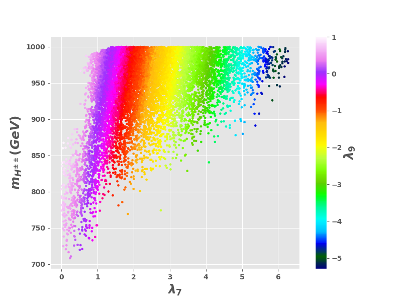
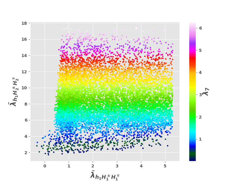
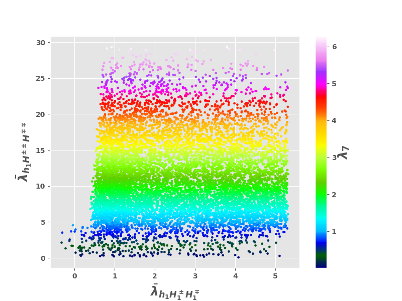
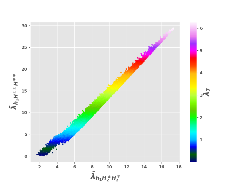
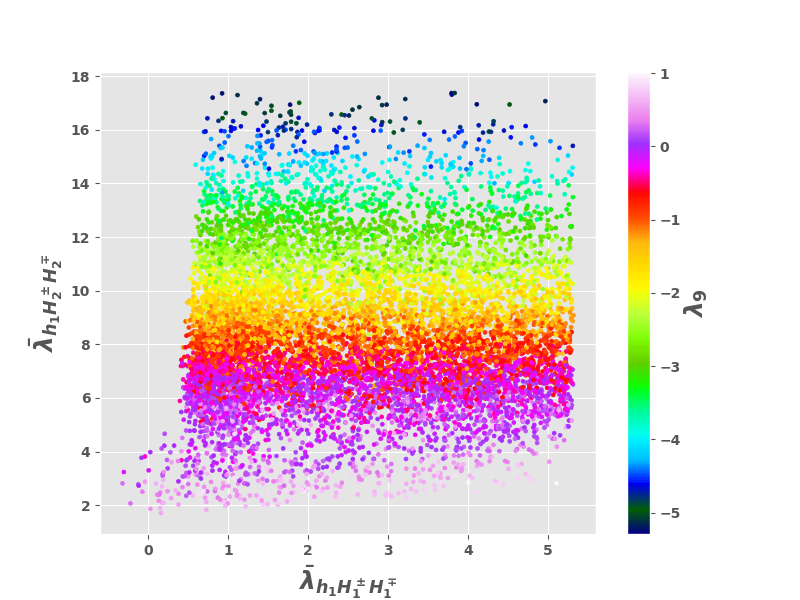
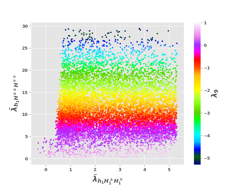
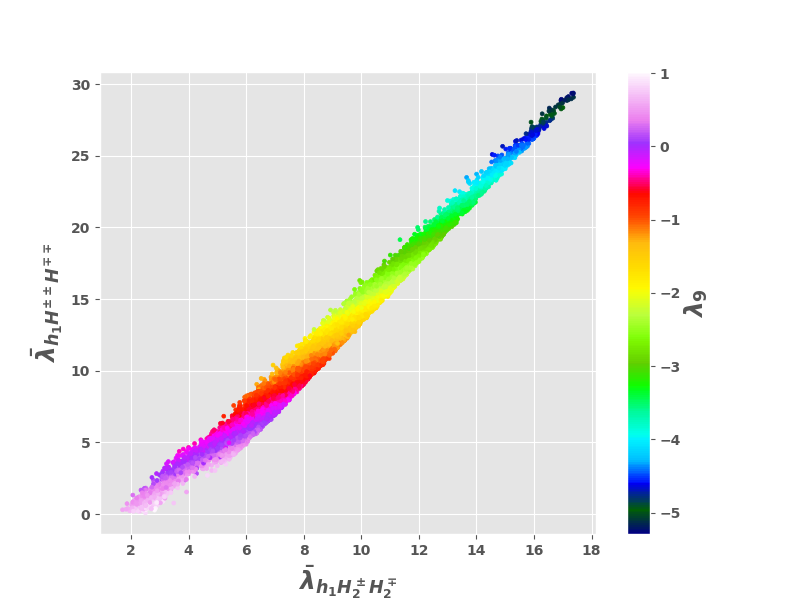
Figure 4: Upper panels: The charged Higgs masses as a function of $\lambda_{7}$ and $\lambda_{9}$ with $m_{H^{\pm}_{1}}$ (left), $m_{H^{\pm}_{2}}$ (middle) and $m_{H^{\pm\pm}}$ (right). Middle panels: correlation between $\bar{\lambda}_{h_{1}H^{\pm}_{1}H^{\mp}_{1}}$ and $\bar{\lambda}_{h_{1}H^{\pm}_{2}H^{\mp}_{2}}$ (left), $\bar{\lambda}_{h_{1}H^{\pm}_{1}H^{\mp}_{1}}$ and $\bar{\lambda}_{h_{1}H^{\pm\pm}H^{\mp\mp}}$ (middle), $\bar{\lambda}_{h_{1}H^{\pm}_{2}H^{\mp}_{2}}$ and $\bar{\lambda}_{h_{1}H^{\pm\pm}H^{\mp\mp}}$ (right) as a function of $\lambda_{7}$. Lower panels: correlation between $\bar{\lambda}_{h_{1}H^{\pm}_{1}H^{\mp}_{1}}$ and $\bar{\lambda}_{h_{1}H^{\pm}_{2}H^{\mp}_{2}}$ (left), $\bar{\lambda}_{h_{1}H^{\pm}_{1}H^{\mp}_{1}}$ and $\bar{\lambda}_{h_{1}H^{\pm\pm}H^{\mp\mp}}$ (middle), $\bar{\lambda}_{h_{1}H^{\pm}_{2}H^{\mp}_{2}}$ and $\bar{\lambda}_{h_{1}H^{\pm\pm}H^{\mp\mp}}$ (right) as a function of $\lambda_{9}$. Here we assume that $\alpha_{1}=1.42$ and $m_{h_{2}}=673.30$  GeV. The other inputs are the same as in (11). The analysis is performed with $\chi^{2}_{ST}$ test where only points that are within $95\%$ confidence level are considered.

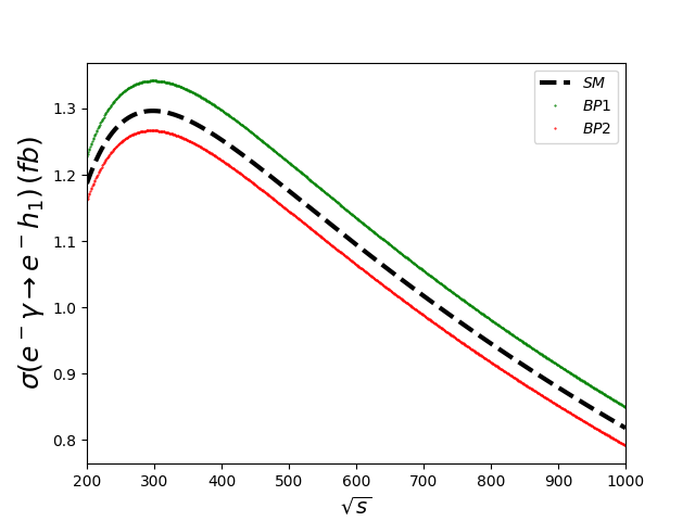
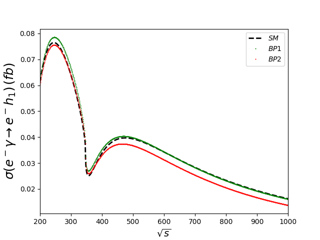
Figure 5: Total unpolarized cross-section in fb for $e^{+}e^{-}\to\gamma h_{1}$ (left) and $e^{-}\gamma\to e^{-}h_{1}$ (right) as a function of center-of-mass energy, in two benchmark scenarios. Here we assume that $\alpha_{1}=1.42$ and $m_{h_{2}}=673.30$  GeV, for the other inputs (see Table 3).

In Fig. 5, we display the unpolarized cross sections of $e^{-}e^{+}\to h_{1}\gamma$ and $e^{-}\gamma\to e^{-}h_{1}$, with respect to the Standard Model one, as a function of $\sqrt{s}$ in the range $200$ to $1000$ GeV. These production cross sections at the linear collider are analyzed for two benchmark scenarios, as illustrated in Table 3. All generated points passed upon the full set of constraints including $B\to X_{s}\gamma$ constraint at 95$\%$ C.L. The corresponding cross sections in the Standard Model are also plotted (dots in black). Our analysis shows that the cross sections of these two processes are very sensitive to the parameters of the model, especially $\alpha_{1}$, $\lambda_{3}$, $\lambda_{7}$ and $\lambda_{9}$, so as expected they are enhanced in the vicinity of $250$ GeV where they get their largest values. Besides we also see that they begin to decline when the detrimental effects of the destructive interference between the Standard Model and 2HDMcT contributions become more pronounced. At this point, we must stress that the constructive or destructive interference with the Standard Model contribution is highly sensitive to the values and signs of the various couplings, $\bar{\lambda}_{h_{1}H^{\pm\pm}H^{\mp\mp}}$,$\bar{\lambda}_{h_{1}H_{1}^{\pm}H_{1}^{\pm}}$,$\bar{\lambda}_{h_{1}H_{2}^{\pm}H_{2}^{\pm}}$ and on $\alpha_{1}$,$\lambda_{3}$,$\lambda_{7}$ and $\lambda_{9}$ parameters. Any change in these couplings (values or signs) could significantly affects the resulting cross sections.

Table 3: Benchmark scenarios used in Fig. 5 where the generated points pass upon the full set of constraints.

Bench.	$\lambda_{1}$	$\lambda_{3}$	$\lambda_{4}$	$\lambda_{6}$	$\lambda_{7}$	$\lambda_{8}$	$\lambda_{9}$	$\bar{\lambda}_{8}$	$\bar{\lambda}_{9}$
BP1	$1.31$	$-0.12$	$1.70$	$0.64$	$0.01$	$0.28$	$0.38$	$2.33$	$0.54$
BP2	$1.31$	$0.80$	$3.06$	$6.04$	$2.15$	$-2.72$	$0.47$	$-1.10$	$3.13$

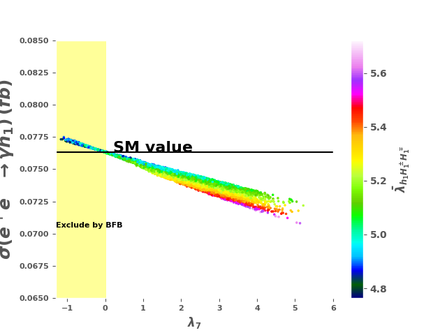
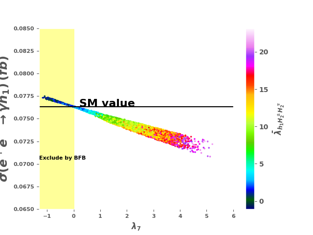
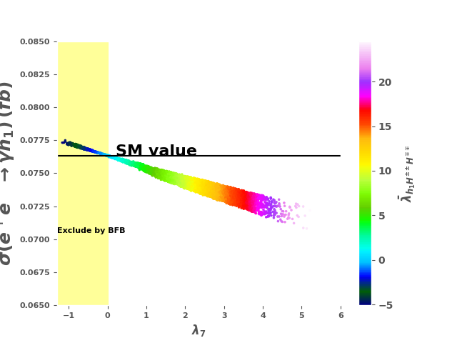
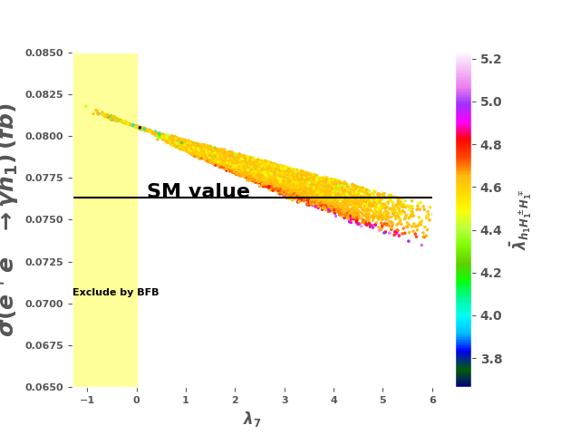
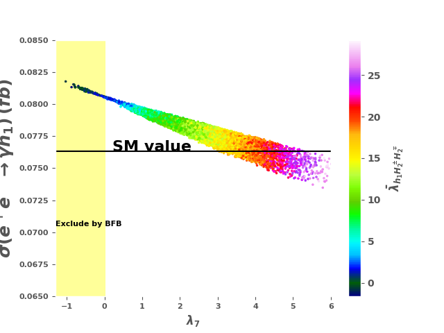
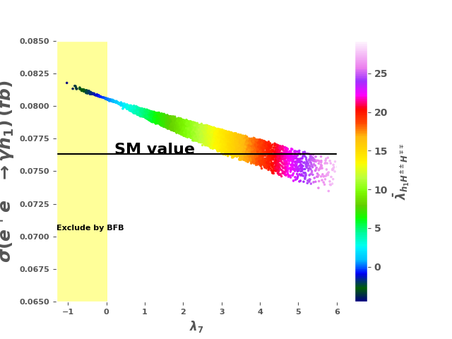
Figure 6: The cross-section $\sigma(e^{+}e^{-}\to\gamma h_{1})$ is depicted as a function of the parameter $\lambda_{7}$ for two values of the parameter $\alpha_{1}$: $\alpha_{1}=1.42$ (upper panels), and $\alpha_{1}=1.44$ (lower panels). The plotted points pass upon all constraints. We used : $\lambda_{1}=1.31$, $\lambda_{3}=6.15$, $\lambda_{4}=-3.85$ and $m_{h_{2}}=673.30$ GeV. The other inputs are the same as in (11). The color coding illustrate the variation of the trilinear couplings $\bar{\lambda}_{h_{1}H^{\pm}_{1}H^{\mp}_{1}}$(left), $\bar{\lambda}_{h_{1}H^{\pm}_{2}H^{\mp}_{2}}$(middle) and $\bar{\lambda}_{h_{1}H^{\pm\pm}H^{\mp\mp}}$ (right panel)

.

Next, we first aim to see whether the diphoton signal strength $R_{\gamma\gamma}(h_{1})$ agrees with the experimental data within the model’s parameter space, knowing that, unlike $h_{1}\to\gamma Z$ process, the decay channel $h_{1}\to\gamma\gamma$, has been measured with high precision [66, 67, 68, 69, 70, 4, 3]. Also, we want to analyze to what extent the cross-section $\sigma(e^{+}e^{-}\to\gamma h_{1})$ behavior is affected either by the $2HDMcT$ charged Higgs bosons or by the potential parameters. Fig. 6 and Fig.7 illustrate the variation of these observables as a function of parameter $\lambda_{7}$, and the trilinear couplings $\bar{\lambda}_{h_{1}H^{+}_{1}H^{-}_{1}}$, $\bar{\lambda}_{h_{1}H^{+}_{2}H^{-}_{2}}$ and $\bar{\lambda}_{h_{1}H^{++}H^{--}}$. It is generally observed that an increase in $\lambda_{7}$ results in detrimental effect on both $R_{\gamma\gamma}$ and $\sigma(e^{+}e^{-}\to\gamma h_{1})$. Similar trend is seen if these observables are plotted versus $\lambda_{3}$.

In Fig.6 we plot the cross-section of $e^{+}e^{-}\to\gamma h_{1}$ process as a function of the parameter $\lambda_{7}$, and the trilinear Higgs couplings for two nearly degenerate values of the parameter $\alpha_{1}$. From the upper panels, with $\alpha_{1}=1.42$, we clearly see that $\sigma(e^{+}e^{-}\to\gamma h_{1})$ undergoes a notable increase and even exceeds the Standard Model prediction if $\lambda_{7}<0$, a region excluded by constraints originating from $BFB$. In this scenario, because of $BFB$ conditions, the contributions of the parameters $\lambda_{6,7,8,9,\bar{8},\bar{9}}$ are rather predominantly detrimental, which induce a decrease in $\sigma(e^{+}e^{-}\to\gamma h_{1})$. More specifically this depreciation stems particularly from the relations, $\lambda_{7}>0$ and $\lambda_{7}+\lambda_{9}>0$, with $\lambda_{7}$ and $\lambda_{9}$ exhibiting contrasting effects. However, if we consider a slightly larger value of the parameter $\alpha_{1}=1.44$, as illustrated by the lower panels, the cross sections experience a significant enhancement and can well surpass that of the Standard Model up to $8.06\,\,10^{-2}$ fb, while still satisfying BFB conditions. On top of that, our results also show that the charged Higgs masses $m_{H^{\pm}_{1}}$, $m_{H^{\pm}_{2}}$ and $m_{H^{\pm\pm}}$ are compelled to lie within the very stringent intervals $[785,790]$ GeV, $[807,990]$ GeV and $[810,995]$ GeV respectively, conforming the predictions reported in  [18].
Next we analyze the signal strengths $R_{\gamma\gamma}$, $R_{\gamma Z}$ and the ratio $R_{\gamma h_{1}}$ within the model parameter space. First, we plot in Fig. 7 the signal strength of the Higgs to diphoton decay as a function of $\lambda_{7}$ parameter, so we observe that $R_{\gamma\gamma}$ is clearly consistent with the measured signal strength[66, 67, 68, 69, 70, 4, 3] at $1\sigma$.

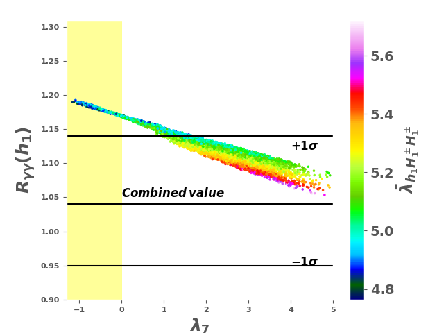
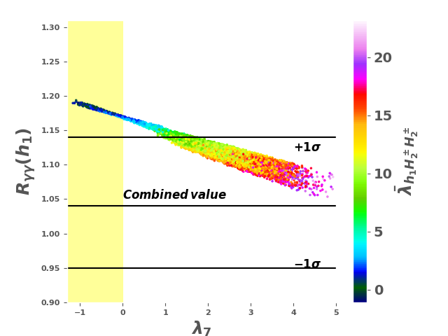
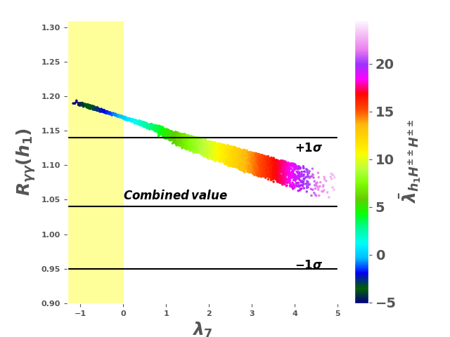
Figure 7: The signal strength $R_{\gamma\gamma}(h_{1})$ as a function of $\lambda_{7}$. The plotted points passed upon all constraints. The color coding shows the variation of the trilinear coupling $\bar{\lambda}_{h_{1}H^{\pm}_{1}H^{\mp}_{1}}$(left), $\bar{\lambda}_{h_{1}H^{\pm}_{2}H^{\mp}_{2}}$(middle) and $\bar{\lambda}_{h_{1}H^{\pm\pm}H^{\mp\mp}}$ (right panel). The displayed horizontal lines denote the central and $\pm 1\sigma$ diphoton strength signal values reported by ATLAS [66, 4] at $13$ TeV. We used the following inputs: $\alpha_{1}=1.42$, $\lambda_{1}=1.31$, $\lambda_{3}=6.15$, $\lambda_{4}=-3.85$ and $m_{h_{2}}=673.30$ GeV. The other inputs are the same as in (11)

, while the error for $\chi^{2}$ fit is 95.5% C.L.

Then, we investigate how $R_{\gamma h_{1}}$ behaves with respect to $R_{\gamma\gamma}$ and $R_{\gamma Z}$ and wether these observables are correlated. One can readily see from Fig. 8 a clear correlation with these two signal strengths. Additionally, we also analyzed the incidence of the doubly charged Higgs on these loop induced processes, via its trilinear Higgs couplings $\bar{\lambda}_{h_{1}H^{\pm\pm}H^{\mp\mp}}$. The results interestingly indicate that the lighter it is, the more significant the enhancement in the total cross-section $\sigma(e^{+}e^{-}\to\gamma h_{1})$, as in $R_{\gamma h_{1}}$ and $R_{\gamma Z}$.

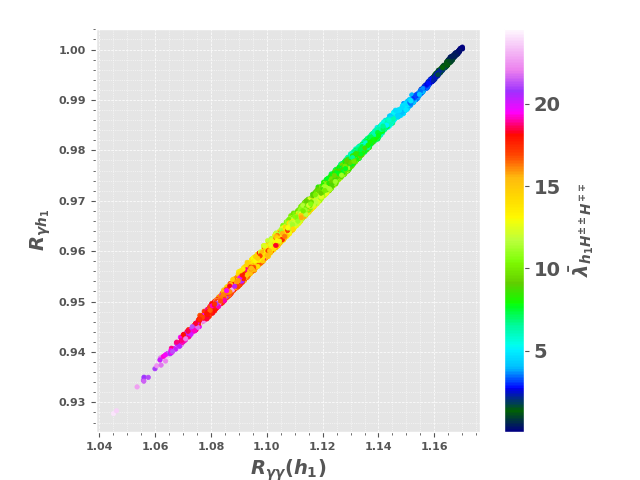
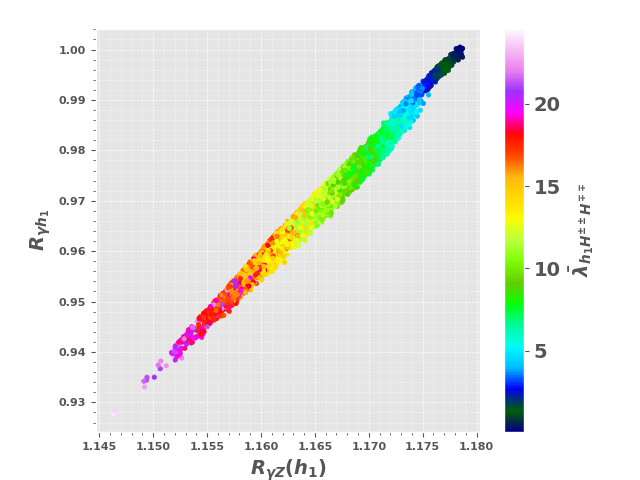
Figure 8: $R_{\gamma h_{1}}$ correlation with $R_{\gamma\gamma}(h_{1})$ (left panels) and $R_{\gamma Z}(h_{1})$ (right panels) in 2HDMcT. Color coding shows the variation of $\bar{\lambda}_{h_{1}H^{\pm\pm}H^{\mp\mp}}$. The inputs are the same as in Fig. 7.

4 CONCLUSION

The future $e^{-}e^{+}$ colliders are anticipated to play a vital role in understanding the nature of the Higgs boson and its coupling to the Standard Model particles with unprecedented precision. In the present paper, we have studied the one-loop processes $e^{+}e^{-}\to\gamma h_{1}$ and $e^{-}\gamma\to e^{-}h_{1}$ in the framework of the two Higgs doublet type-II seesaw model (2HDMcT) at the $e^{-}e^{+}$ colliders, where the $h_{1}$ Higgs boson is chosen to replicate the observed Higgs. Within the $2HDMcT$ parameter space delimited by a full set of constraints, we have shown that the $2HDMcT$ charged scalars can substantially alter the cross sections $\sigma(e^{+}e^{-}\to\gamma h_{1})$ and $\sigma(e^{-}\gamma\to e^{-}h_{1})$. Our analysis also observed that these observables are especially sensitive to the parameters $\alpha_{1}$, $\lambda_{7}$, $\lambda_{9}$, the trilinear Higgs couplings as to the charged scalars masses. These parameters conspire to induce significant contributions to $\sigma(e^{+}e^{-}\to h_{1}\gamma)$, up to $8.1\times 10^{-2}$ fb so exceeding the Standard Model prediction.

Additionally, the charged scalars $H_{1}^{\pm}$, $H_{2}^{\pm}$ and $H^{\pm\pm}$ also affected the ratio $R_{h_{1}\gamma}$ and the signal strength $R_{Z\gamma}$, while $R_{\gamma\gamma}$ being consistent with the measured signal strength at $1\sigma$. Besides, another outcome of our study imply that these three observables are entirely correlated with each other.

References

- [1] ATLAS Collaboration, G. Aad et al., Observation of a new particle in the search for the Standard Model Higgs boson with the ATLAS detector at the LHC, Phys. Lett. B 716 (2012) 1–29, [arXiv:1207.7214].
- [2] CMS Collaboration, S. Chatrchyan et al., Observation of a New Boson at a Mass of 125 GeV with the CMS Experiment at the LHC, Phys. Lett. B 716 (2012) 30–61, [arXiv:1207.7235].
- [3] CMS Collaboration, A. Tumasyan et al., A portrait of the Higgs boson by the CMS experiment ten years after the discovery., Nature 607 (2022), no. 7917 60–68, [arXiv:2207.00043].
- [4] ATLAS Collaboration, G. Aad et al., A detailed map of Higgs boson interactions by the ATLAS experiment ten years after the discovery, Nature 607 (2022), no. 7917 52–59, [arXiv:2207.00092]. [Erratum: Nature 612, E24 (2022)].
- [5] W. Elmetenawee, Summary of CMS Higgs Physics, arXiv:2401.07650.
- [6] F. Zwicky, Die Rotverschiebung von extragalaktischen Nebeln, Helv. Phys. Acta 6 (1933) 110–127.
- [7] V. C. Rubin and W. K. Ford, Jr., Rotation of the Andromeda Nebula from a Spectroscopic Survey of Emission Regions, Astrophys. J. 159 (1970) 379–403.
- [8] M. J. G. Veltman, The Infrared - Ultraviolet Connection, Acta Phys. Polon. B 12 (1981) 437.
- [9] T. Kajita, Nobel lecture: Discovery of atmospheric neutrino oscillations, Rev. Mod. Phys. 88 (Jul, 2016) 030501.
- [10] A. B. McDonald, Nobel lecture: The sudbury neutrino observatory: Observation of flavor change for solar neutrinos, Rev. Mod. Phys. 88 (Jul, 2016) 030502.
- [11] N. G. Deshpande and E. Ma, Pattern of Symmetry Breaking with Two Higgs Doublets, Phys. Rev. D 18 (1978) 2574.
- [12] S. L. Glashow and S. Weinberg, Natural conservation laws for neutral currents, Phys. Rev. D 15 (Apr, 1977) 1958–1965.
- [13] G. C. Branco, P. M. Ferreira, L. Lavoura, M. N. Rebelo, M. Sher, and J. P. Silva, Theory and phenomenology of two-Higgs-doublet models, Phys. Rept. 516 (2012) 1–102, [arXiv:1106.0034].
- [14] S. Dawson, C. Englert, and T. Plehn, Higgs Physics: It ain’t over till it’s over, Phys. Rept. 816 (2019) 1–85, [arXiv:1808.01324].
- [15] I. P. Ivanov, Building and testing models with extended Higgs sectors, Prog. Part. Nucl. Phys. 95 (2017) 160–208, [arXiv:1702.03776].
- [16] S. Weinberg, Baryon- and lepton-nonconserving processes, Phys. Rev. Lett. 43 (Nov, 1979) 1566–1570.
- [17] B. Ait Ouazghour, A. Arhrib, R. Benbrik, M. Chabab, and L. Rahili, Theory and phenomenology of a two-Higgs-doublet type-II seesaw model at the LHC run 2, Phys. Rev. D 100 (2019), no. 3 035031, [arXiv:1812.07719].
- [18] B. Ait Ouazghour and M. Chabab, The two Higgs doublet type-II seesaw model: Naturalness and B¯→Xs versus heavy Higgs masses, Phys. Lett. B 846 (2023) 138241, [arXiv:2305.08030].
- [19] ATLAS Collaboration, M. Aaboud et al., Search for additional heavy neutral Higgs and gauge bosons in the ditau final state produced in 36 fb-1 of pp collisions at TeV with the ATLAS detector, JHEP 01 (2018) 055, [arXiv:1709.07242].
- [20] ATLAS Collaboration, M. Aaboud et al., Search for new phenomena in high-mass diphoton final states using 37 fb-1 of proton–proton collisions collected at TeV with the ATLAS detector, Phys. Lett. B 775 (2017) 105–125, [arXiv:1707.04147].
- [21] CMS Collaboration, A. M. Sirunyan et al., Search for a new scalar resonance decaying to a pair of Z bosons in proton-proton collisions at TeV, JHEP 06 (2018) 127, [arXiv:1804.01939]. [Erratum: JHEP 03, 128 (2019)].
- [22] ATLAS Collaboration, M. Aaboud et al., Search for a heavy Higgs boson decaying into a boson and another heavy Higgs boson in the final state in collisions at TeV with the ATLAS detector, Phys. Lett. B 783 (2018) 392–414, [arXiv:1804.01126].
- [23] CMS Collaboration, A. M. Sirunyan et al., Search for heavy Higgs bosons decaying to a top quark pair in proton-proton collisions at 13 TeV, JHEP 04 (2020) 171, [arXiv:1908.01115]. [Erratum: JHEP 03, 187 (2022)].
- [24] CMS Collaboration, A. M. Sirunyan et al., Search for MSSM Higgs bosons decaying to + in proton-proton collisions at s=13TeV, Phys. Lett. B 798 (2019) 134992, [arXiv:1907.03152].
- [25] CMS Collaboration, Search for a charged Higgs boson decaying into a heavy neutral Higgs boson and a W boson in proton-proton collisions at = 13 TeV, arXiv e-prints (July, 2022) arXiv:2207.01046, [arXiv:2207.01046].
- [26] R. S. Gupta, H. Rzehak, and J. D. Wells, How well do we need to measure the Higgs boson mass and self-coupling?, Phys. Rev. D 88 (2013) 055024, [arXiv:1305.6397].
- [27] J. Baglio and C. Weiland, The triple Higgs coupling: A new probe of low-scale seesaw models, JHEP 04 (2017) 038, [arXiv:1612.06403].
- [28] ILC physics, detector study Collaboration, J. Tian and K. Fujii, Measurement of Higgs boson couplings at the International Linear Collider, Nucl. Part. Phys. Proc. 273-275 (2016) 826–833.
- [29] C. F. Dürig, Measuring the Higgs Self-coupling at the International Linear Collider. PhD thesis, Hamburg U., Hamburg, 2016.
- [30] T. Liu, K.-F. Lyu, J. Ren, and H. X. Zhu, Probing the quartic Higgs boson self-interaction, Phys. Rev. D 98 (2018), no. 9 093004, [arXiv:1803.04359].
- [31] A. Arbey et al., Physics at the e+ e- Linear Collider, Eur. Phys. J. C 75 (2015), no. 8 371, [arXiv:1504.01726].
- [32] ILC International Development Team Collaboration, A. Aryshev et al., The International Linear Collider: Report to Snowmass 2021, arXiv:2203.07622.
- [33] P. Bambade et al., The International Linear Collider: A Global Project, arXiv:1903.01629.
- [34] CLIC Physics Working Group Collaboration, E. Accomando et al., Physics at the CLIC multi-TeV linear collider, in 11th International Conference on Hadron Spectroscopy, CERN Yellow Reports: Monographs, 6, 2004. hep-ph/0412251.
- [35] CEPC Study Group Collaboration, CEPC Conceptual Design Report: Volume 1 - Accelerator, arXiv:1809.00285.
- [36] CEPC Study Group Collaboration, M. Dong et al., CEPC Conceptual Design Report: Volume 2 - Physics & Detector, arXiv:1811.10545.
- [37] CEPC Study Group Collaboration, W. Abdallah et al., CEPC Technical Design Report – Accelerator, arXiv:2312.14363.
- [38] TLEP Design Study Working Group Collaboration, M. Bicer et al., First Look at the Physics Case of TLEP, JHEP 01 (2014) 164, [arXiv:1308.6176].
- [39] FCC Collaboration, A. Abada et al., FCC Physics Opportunities: Future Circular Collider Conceptual Design Report Volume 1, Eur. Phys. J. C 79 (2019), no. 6 474.
- [40] LCC Physics Working Group Collaboration, K. Fujii et al., Tests of the Standard Model at the International Linear Collider, arXiv:1908.11299.
- [41] A. Abbasabadi, D. Bowser-Chao, D. A. Dicus, and W. W. Repko, Higgs-boson–photon associated production at eē colliders, Phys. Rev. D 52 (Oct, 1995) 3919–3928.
- [42] A. Djouadi, V. Driesen, W. Hollik, and J. Rosiek, Associated production of Higgs bosons and a photon in high-energy e+e- collisions, Nuclear Physics B 491 (Feb., 1997) 68–102, [hep-ph/9609420].
- [43] A. Barroso, J. Pulido, and J. C. Romao, HIGGS PRODUCTION AT e+ e- COLLIDERS, Nucl. Phys. B 267 (1986) 509–530.
- [44] A. Arhrib, R. Benbrik, and T.-C. Yuan, Associated Production of Higgs at Linear Collider in the Inert Higgs Doublet Model, Eur. Phys. J. C 74 (2014) 2892, [arXiv:1401.6698].
- [45] L. Rahili, A. Arhrib, and R. Benbrik, Associated production of SM Higgs with a photon in type-II seesaw models at the ILC, Eur. Phys. J. C 79 (2019), no. 11 940, [arXiv:1909.07793].
- [46] S. Heinemeyer and C. Schappacher, Neutral Higgs boson production at e+̂e-̂ colliders in the complex MSSM: a full one-loop analysis, European Physical Journal C 76 (Apr., 2016) 220, [arXiv:1511.06002].
- [47] M. Demirci, Associated production of Higgs boson with a photon at electron-positron colliders, Phys. Rev. D 100 (2019), no. 7 075006, [arXiv:1905.09363].
- [48] ILD concept group Collaboration, Y. Aoki, K. Fujii, and J. Tian, Study of at the ILC, arXiv:2203.07202.
- [49] M. J. Ramsey-Musolf, The electroweak phase transition: a collider target, JHEP 09 (2020) 179, [arXiv:1912.07189].
- [50] M. E. Peskin and T. Takeuchi, Estimation of oblique electroweak corrections, Phys. Rev. D46 (1992) 381–409.
- [51] W. Grimus, L. Lavoura, O. M. Ogreid, and P. Osland, The Oblique parameters in multi-Higgs-doublet models, Nucl. Phys. B 801 (2008) 81–96, [arXiv:0802.4353].
- [52] Particle Data Group Collaboration, P. A. Zyla et al., Review of Particle Physics, PTEP 2020 (2020), no. 8 083C01.
- [53] H. Bahl, T. Biekötter, S. Heinemeyer, C. Li, S. Paasch, G. Weiglein, and J. Wittbrodt, HiggsTools: BSM scalar phenomenology with new versions of HiggsBounds and HiggsSignals, Comput. Phys. Commun. 291 (2023) 108803, [arXiv:2210.09332].
- [54] P. Bechtle, S. Heinemeyer, O. Stål, T. Stefaniak, and G. Weiglein, : Confronting arbitrary Higgs sectors with measurements at the Tevatron and the LHC, Eur. Phys. J. C 74 (2014), no. 2 2711, [arXiv:1305.1933].
- [55] P. Bechtle, S. Heinemeyer, O. Stål, T. Stefaniak, and G. Weiglein, Probing the Standard Model with Higgs signal rates from the Tevatron, the LHC and a future ILC, JHEP 11 (2014) 039, [arXiv:1403.1582].
- [56] P. Bechtle, S. Heinemeyer, T. Klingl, T. Stefaniak, G. Weiglein, and J. Wittbrodt, HiggsSignals-2: Probing new physics with precision Higgs measurements in the LHC 13 TeV era, Eur. Phys. J. C 81 (2021), no. 2 145, [arXiv:2012.09197].
- [57] P. Bechtle, O. Brein, S. Heinemeyer, G. Weiglein, and K. E. Williams, HiggsBounds: Confronting Arbitrary Higgs Sectors with Exclusion Bounds from LEP and the Tevatron, Comput. Phys. Commun. 181 (2010) 138–167, [arXiv:0811.4169].
- [58] P. Bechtle, O. Brein, S. Heinemeyer, G. Weiglein, and K. E. Williams, HiggsBounds 2.0.0: Confronting Neutral and Charged Higgs Sector Predictions with Exclusion Bounds from LEP and the Tevatron, Comput. Phys. Commun. 182 (2011) 2605–2631, [arXiv:1102.1898].
- [59] P. Bechtle, O. Brein, S. Heinemeyer, O. Stål, T. Stefaniak, G. Weiglein, and K. E. Williams, : Improved Tests of Extended Higgs Sectors against Exclusion Bounds from LEP, the Tevatron and the LHC, Eur. Phys. J. C 74 (2014), no. 3 2693, [arXiv:1311.0055].
- [60] P. Bechtle, D. Dercks, S. Heinemeyer, T. Klingl, T. Stefaniak, G. Weiglein, and J. Wittbrodt, HiggsBounds-5: Testing Higgs Sectors in the LHC 13 TeV Era, Eur. Phys. J. C 80 (2020), no. 12 1211, [arXiv:2006.06007].
- [61] HFLAV Collaboration, Y. S. Amhis et al., Averages of -hadron, -hadron, and -lepton properties as of 2021, Phys. Rev. D 107 (2023) 052008, [arXiv:2206.07501].
- [62] T. Hahn, Generating Feynman diagrams and amplitudes with FeynArts 3, Comput. Phys. Commun. 140 (2001) 418–431, [hep-ph/0012260].
- [63] T. Hahn and M. Pérez-Victoria, Automated one-loop calculations in four and d dimensions, Computer Physics Communications 118 (1999), no. 2 153–165.
- [64] G. J. van Oldenborgh, FF: A Package to evaluate one loop Feynman diagrams, Comput. Phys. Commun. 66 (1991) 1–15.
- [65] T. Hahn, Feynman Diagram Calculations with FeynArts, FormCalc, and LoopTools, PoS ACAT2010 (2010) 078, [arXiv:1006.2231].
- [66] ATLAS Collaboration, G. Aad et al., Measurement of the properties of Higgs boson production at TeV in the channel using fb-1 of collision data with the ATLAS experiment, JHEP 07 (2023) 088, [arXiv:2207.00348].
- [67] ATLAS Collaboration, G. Aad et al., A search for the decay mode of the Higgs boson in collisions at = 13 TeV with the ATLAS detector, Phys. Lett. B 809 (2020) 135754, [arXiv:2005.05382].
- [68] CMS Collaboration, A. Tumasyan et al., Search for Higgs boson decays to a Z boson and a photon in proton-proton collisions at = 13 TeV, JHEP 05 (2023) 233, [arXiv:2204.12945].
- [69] CMS, ATLAS Collaboration, G. Aad et al., Evidence for the Higgs boson decay to a boson and a photon at the LHC, arXiv:2309.03501.
- [70] ATLAS Collaboration, G. Aad et al., Search for the decay mode of new high-mass resonances in collisions at TeV with the ATLAS detector, arXiv:2309.04364.