Tightly Bounded Polynomials via Flexible Discretizations for Dynamic Optimization Problems*

Abstract

Polynomials are widely used to represent the trajectories of states and/or inputs. It has been shown that a polynomial can be bounded by its coefficients, when expressed in the Bernstein basis. However, in general, the bounds provided by the Bernstein coefficients are not tight. We propose a method for obtaining numerical solutions to dynamic optimization problems, where a flexible discretization is used to achieve tight polynomial bounds. The proposed method is used to solve a constrained cart-pole swing-up optimal control problem. The flexible discretization eliminates the conservatism of the Bernstein bounds and enables a lower cost, in comparison with non-flexible discretizations. A theoretical result on obtaining tight polynomial bounds with a finite discretization is presented. In some applications with linear dynamics, the non-convexity introduced by the flexible discretization may be a drawback.

I Introduction

Polynomials can approximate most continuous functions to arbitrarily high precision, with sharp rates of convergence. Hence, polynomials are widely used to represent the trajectories of states and/or inputs. However, it can be challenging to ensure that a polynomial $p$ satisfies lower and upper constraints, $p_{\ell}$ and $p_{u}$ respectively, throughout a finite interval $[t_{a},t_{b}]$, i.e.

$$p_{\ell}\leq p(t)\leq p_{u}\quad\forall t\in[t_{a},t_{b}].$$ (1)

Often, only a finite number of samples of $p$ are constrained, with no guarantee of constraint satisfaction in-between samples.

To rigorously enforce (1), one may naively consider constraining the extrema of $p$. While the roots of 1^st or 2^nd degree polynomials can be easily obtained, for 3^rd and 4^th degrees the expressions grow significantly, and for 5^th or higher degrees there are no closed-form expressions. A less futile strategy is to use sum-of-squares (SOS) conditions to enforce non-negativity of a polynomial over a finite interval [1, Sect. 1.21]. However, SOS conditions are formulated as semi-definite programming constraints, which require specialized solution techniques.

A simpler approach is to express $p$ in the Bernstein polynomial basis, where a set of linear constraints on the coefficients is sufficient to ensure that (1) is satisfied [2]. In general, the bounds provided by the Bernstein coefficients are not tight, i.e. they are potentially conservative approximations of the true minimum and maximum values of $p$ in $[t_{a},t_{b}]$.

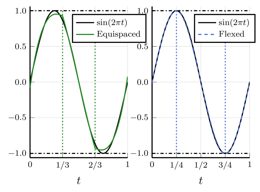
Figure 1: Bernstein-constrained piecewise polynomial approximations with equispaced and flexed sub-intervals.

The conservatism of the Bernstein bounds is illustrated by a simple approximation problem. The function

$$t\mapsto\sin(2\pi t),\quad t\in[0,1]$$ (2)

is approximated by continuous piecewise polynomials with their Bernstein coefficients constrained between -1 and 1 (the remaining details can be found in the Appendix). Figure 1 shows how the bounds may or may not be tight, depending on how the interval $[0,1]$ is partitioned. With equispaced sub-intervals, the Bernstein bounds on the polynomials are not tight, resulting in a significant approximation error near the constraints. With an appropriate flexing of the sub-intervals, the bounds become tight, and the approximation error is greatly reduced.

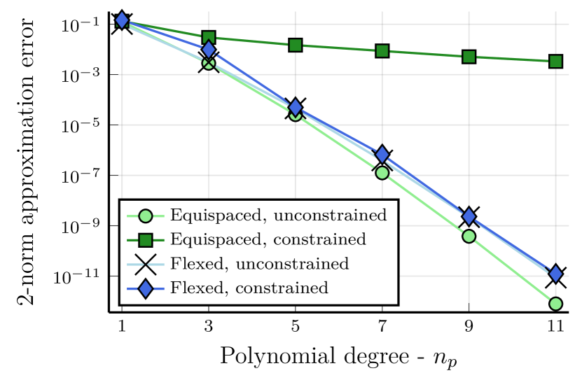
Figure 2: Approximation errors for equispaced and flexed sub-intervals, with and without Bernstein constraints.

Figure 2 shows how conservative Bernstein bounds can impact the rate of convergence of the approximation error. With equispaced sub-intervals, the constraints hinder the otherwise sharp rate of convergence, whereas with flexed sub-intervals, the unconstrained rate of convergence is mostly preserved.

In this article, the idea of obtaining tight polynomial bounds using flexible sub-intervals is presented for a larger class of problems. The class of dynamic optimization problems (DOPs) is concerned with finding states and inputs that minimize a given cost function, while subject to various constraints. Optimal control problems, as well as state estimation and system identification problems can all be formulated as DOPs. Moreover, initial value problems and boundary value problems of differential (algebrai(c) equations are also sub-classes of DOPs.

Pseudo-spectral collocation methods are the state of the art for numerically solving DOPs. By using certain families of polynomials, these methods can obtain an exponential rate of convergence, known as the spectral rate. Recently, pseudo-spectral methods based on Birkhoff interpolation have been shown to greatly improve the numerical conditioning, in contrast with traditional Lagrange interpolation [3]. Generally, pseudo-spectral methods do not rigorously enforce polynomial constraints as in (1), instead only constraining samples of the polynomial values.

A non-pseudo-spectral collocation method purely based on Bernstein polynomials has been proposed for DOPs [4]. Despite the advantageous constraint satisfaction properties, the method results in a slower rate of convergence. A pseudo-spectral method that uses Bernstein constraints has been proposed [5], capable of attaining a spectral rate of convergence. Later, the method was extended to use fixed sub-intervals [6], so as to reduce (but not eliminate) the conservatism of the Bernstein constraints.

In this article, the proposed pseudo-spectral DOP method uses flexible sub-intervals to achieve tight polynomial bounds, thus eliminating the conservatism of Bernstein constraints. Previously, the use of flexible sub-intervals has been associated with capturing discontinuities in the solutions, both in collocation methods [7] and in integrated-residual methods [8].

The contributions of this article are the following:

• We propose a method for obtaining numerical solutions to DOPs, where a flexible discretization is used to allow for tight polynomial bounds to be achieved;

• We show that monotonic polynomials can be partitioned into a finite number of sub-intervals, where the polynomial of each sub-interval can be tightly bounded.

Section II describes the discretizations of each element of a DOP. Section III presents the Bernstein basis, along with the theoretical result on tight polynomial bounds. In Section IV the proposed method is applied to a cart-pole swing-up problem. Section V provides concluding remarks and directions for further research.

II Problem Discretization

II-A Dynamic Optimization Problem

We define a DOP as finding the $n_{x}$ continuous states $\boldsymbol{x}:[t_{0},t_{f}]\rightarrow\mathbb{R}^{n_{x}}$ and $n_{u}$ inputs $\boldsymbol{u}:[t_{0},t_{f}]\rightarrow\mathbb{R}^{n_{u}}$ that

$$\begin{array}[]{rlr}\text{minimize}&\lx@intercol m(\boldsymbol{x}(t_{0}),\boldsymbol{x}(t_{f}))+\displaystyle{\int_{t_{0}}^{t_{f}}\ell(\boldsymbol{x}(t),\boldsymbol{u}(t),t)\textrm{d}t,}\hfil\lx@intercol\\ \text{subject to}&b(\boldsymbol{x}(t_{0}),\boldsymbol{x}(t_{f}))=0,\\ &r(\dot{\boldsymbol{x}}(t),\boldsymbol{x}(t),\boldsymbol{u}(t),t)=0&\widetilde{\forall}t\in[t_{0},t_{f}],\\ &\boldsymbol{x}(t)\in\mathbb{X},\,\boldsymbol{u}(t)\in\mathbb{U}&\forall t\in[t_{0},t_{f}].\end{array}$$ (P)

The cost function includes a boundary cost $m:\mathbb{R}^{n_{x}}\times\mathbb{R}^{n_{x}}\rightarrow\mathbb{R}$ and a time-integrated cost $\ell:\mathbb{R}^{n_{x}}\times\mathbb{R}^{n_{u}}\times[t_{0},t_{f}]\rightarrow\mathbb{R}$. As equality constraints, $b:\mathbb{R}^{n_{x}}\times\mathbb{R}^{n_{x}}\rightarrow\mathbb{R}^{n_{b}}$ includes the $n_{b}$ boundary conditions and $r:\mathbb{R}^{n_{x}}\times\mathbb{R}^{n_{x}}\times\mathbb{R}^{n_{u}}\times[t_{0},t_{f}]\rightarrow\mathbb{R}^{n_{r}}$ includes the $n_{r}$ dynamic equations. The latter are only enforced almost-everywhere ($\widetilde{\forall}$) due the partitioning of $[t_{0},t_{f}]$ into sub-intervals, as described in the next sub-section. The sets $\mathbb{X}$ and $\mathbb{U}$ include simple inequality constraints for the states and inputs

$$\mathbb{X} :=\{z\in\mathbb{R}^{n_{x}}\,|\,x_{\ell}\leq z\leq x_{u}\},$$ (3)

$$\mathbb{U} :=\{z\in\mathbb{R}^{n_{u}}\,|\,u_{\ell}\leq z\leq u_{u}\},$$ (4)

where $x_{\ell},x_{u}\in\mathbb{R}^{n_{x}}$ and $u_{\ell},u_{u}\in\mathbb{R}^{n_{u}}$ are the respective lower and upper constraint values. General inequality constraints of the form

$$g_{\ell}\leq g(\dot{\boldsymbol{x}}(t),\boldsymbol{x}(t),\boldsymbol{u}(t),t)\leq g_{u}\quad\widetilde{\forall}t\in[t_{0},t_{f}]$$ (5)

can be included into (P) by incorporating

$$g(\dot{\boldsymbol{x}}(t),\boldsymbol{x}(t),\boldsymbol{u}(t),t)-\boldsymbol{s}(t)=0\quad\widetilde{\forall}t\in[t_{0},t_{f}]$$ (6)

in the dynamic equations, with the slack input variables $\boldsymbol{s}$ constrained by $g_{\ell}$ and $g_{u}$.

The method presented in this article can be easily extended to broader classes of DOPs, such as those with variable $t_{0}$ and $t_{f}$, system parameters, and multiple phases.

II-B Flexible Sub-Intervals

Typically, the interval $[t_{0},t_{f}]$ is partitioned into $n_{h}$ fixed sub-intervals, defined by the values

$$t_{0}<t_{1}<t_{2}<...<t_{n_{h}-1}<t_{f}.$$ (7)

Alternatively, $[t_{0},t_{f}]$ can be partitioned into $n_{h}$ flexible sub-intervals, defined by

$$t_{0}<\stackrel{{\scriptstyle\leftrightarrow}}{{t}}_{1}<\stackrel{{\scriptstyle\leftrightarrow}}{{t}}_{2}<...<\stackrel{{\scriptstyle\leftrightarrow}}{{t}}_{n_{h}-1}<t_{f},$$ (8)

where $\{\stackrel{{\scriptstyle\leftrightarrow}}{{t}}_{i}\}_{i=1}^{n_{h}-1}$ are optimization variables. It is often useful to restrict the sizes of the flexible sub-intervals. We define the flexibility parameters $\{\phi_{i}\}_{i=1}^{n_{h}}$, each within $[0,1)$, to include the inequality constraints

$$(1-\phi_{i})(t_{i}-t_{i-1})\leq\stackrel{{\scriptstyle\leftrightarrow}}{{t}}_{i}-\stackrel{{\scriptstyle\leftrightarrow}}{{t}}_{i-1}\leq\phi_{i}(t_{f}-t_{0})+\\ (1-\phi_{i})(t_{i}-t_{i-1})$$ (9)

for each sub-interval $i\in\{1,2,...,n_{h}\}$, where $\stackrel{{\scriptstyle\leftrightarrow}}{{t}}_{0}\,\equiv t_{0}$ and $\stackrel{{\scriptstyle\leftrightarrow}}{{t}}_{n_{h}}\,\equiv t_{f}$. In the special case where all flexibility parameters $\{\phi_{i}\}_{i=1}^{n_{h}}$ equal 0%, the fixed partitioning (7) is recovered.

II-C Dynamic Variables

For the $i^{\text{th}}$ (flexible) interval, the states and inputs are discretized by interpolating polynomials. To simplify notation, the interpolations are defined in the normalized time domain $\tau\in[-1,1]$, mapped to $t\in[\stackrel{{\scriptstyle\leftrightarrow}}{{t}}_{i-1},\stackrel{{\scriptstyle\leftrightarrow}}{{t}}_{i}]$ via

$$\gamma(\tau;\stackrel{{\scriptstyle\leftrightarrow}}{{t}}_{i-1},\stackrel{{\scriptstyle\leftrightarrow}}{{t}}_{i}):=\frac{\stackrel{{\scriptstyle\leftrightarrow}}{{t}}_{i}-\stackrel{{\scriptstyle\leftrightarrow}}{{t}}_{i-1}}{2}\tau+\frac{\stackrel{{\scriptstyle\leftrightarrow}}{{t}}_{i-1}+\stackrel{{\scriptstyle\leftrightarrow}}{{t}}_{i}}{2}.$$ (10)

Using a Legendre-Gauss-Radau (LGR) collocation method of degree $n$, the interpolation points $\{\tau_{j}\}_{j=0}^{n}$ are the $n$ LGR collocation points, with the extra point $\tau_{n}=1$.

The function $\widetilde{x}_{n}:\mathbb{[}{-}1,1]\times\mathbb{R}^{(n+1)\times n_{x}}\rightarrow\mathbb{R}^{n_{x}}$ approximates the states with $n_{x}$ Lagrange interpolating polynomials of degree $n$,

$$\widetilde{x}_{n}(\tau;x_{i}):=\sum_{j=0}^{n}\Bigg{(}x_{i,j}\prod_{\begin{subarray}{c}k=0\\ k\neq j\end{subarray}}^{n}\frac{\tau-\tau_{k}}{\tau_{j}-\tau_{k}}\Bigg{)},$$ (11)

where $x_{i,j}$ are the states at the $j^{\text{th}}$ interpolation point of the $i^{\text{th}}$ sub-interval and $x_{i}$ is $\{x_{i,j}\}_{j=0}^{n}$. The continuity between sub-intervals is preserved by enforcing

$$\widetilde{x}_{n}(1,x_{i})=\widetilde{x}_{n}(-1;x_{i-1}),$$ (12)

for $i\in\{2,...,n_{h}\}$. The function $\widetilde{u}_{n}:\mathbb{[}{-}1,1]\times\mathbb{R}^{n\times n_{u}}\rightarrow\mathbb{R}^{n_{u}}$ approximates the inputs with $n_{u}$ Lagrange interpolating polynomials of degree $n-1$,

$$\widetilde{u}_{n}(\tau;x_{i}):=\sum_{j=0}^{n-1}\Bigg{(}u_{i,j}\prod_{\begin{subarray}{c}k=0\\ k\neq j\end{subarray}}^{n-1}\frac{\tau-\tau_{k}}{\tau_{j}-\tau_{k}}\Bigg{)},$$ (13)

where $u_{i,j}$ are the inputs at the $j^{\text{th}}$ collocation point of the $i^{\text{th}}$ sub-interval and $u_{i}$ is $\{u_{i,j}\}_{j=0}^{n-1}$. Figure 3 exemplifies the discretization of the dynamic variables in flexible sub-intervals.

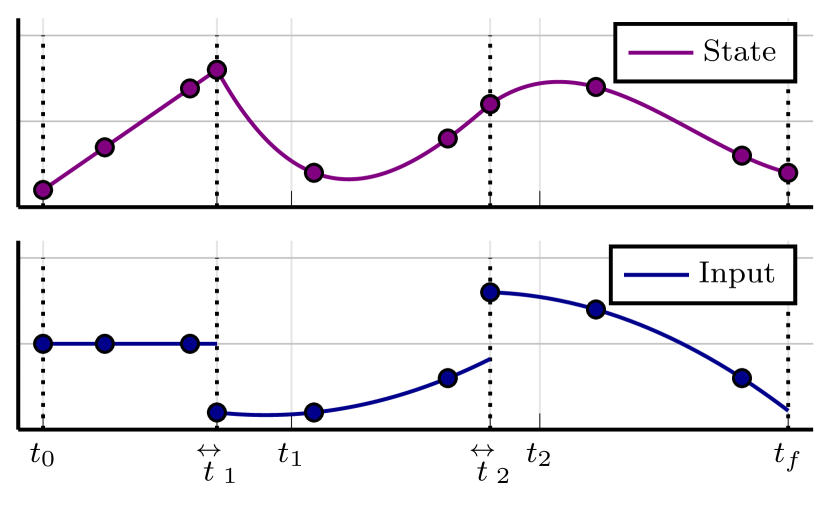
Figure 3: Representations of flexible state and input discretizations for an LGR collocation method of degree $n=3$.

Other variants of pseudo-spectral methods can also be used, such as those based on Chebyshev polynomials. Additionally, pseudo-spectral methods based on Birkhoff interpolation [3] are also compatible with the proposed framework.

II-D Cost Function

The boundary cost of the discretized states is simply

$$m(\widetilde{x}_{n}(-1;x_{0}),\widetilde{x}_{n}(1;x_{n_{h}})).$$ (14)

The time-integrated cost is numerically approximated by Gaussian quadrature as

$$\sum_{i=1}^{n_{h}}\frac{\stackrel{{\scriptstyle\leftrightarrow}}{{t}}_{i}-\stackrel{{\scriptstyle\leftrightarrow}}{{t}}_{i-1}}{2}\sum_{j=0}^{n-1}w_{j}\ell\Big{(}\widetilde{x}_{n}(\tau_{j};x_{i}),\\ \widetilde{u}_{n}(\tau_{j};u_{i}),\gamma\Big{(}\tau_{j},\stackrel{{\scriptstyle\leftrightarrow}}{{t}}_{i-1},\stackrel{{\scriptstyle\leftrightarrow}}{{t}}_{i}\Big{)}\Big{)},$$ (15)

where $\{\tau_{j}\}_{j=0}^{n-1}$ and $\{w_{j}\}_{j=0}^{n-1}$ are the $n$ LGR quadrature points and weights, respectively.

II-E Equality Constraints

The boundary conditions of the discretized states are simply enforced by

$$b(\widetilde{x}_{n}(-1;x_{0}),\widetilde{x}_{n}(1;x_{n_{h}}))=0.$$ (16)

The dynamic equations are enforced at every collocation point $\{\tau_{j}\}_{j=0}^{n-1}$ by setting

$$r\Bigg{(}\frac{2\dot{\widetilde{x}}_{n}(\tau_{j};x_{i})}{\stackrel{{\scriptstyle\leftrightarrow}}{{t}}_{i}-\stackrel{{\scriptstyle\leftrightarrow}}{{t}}_{i-1}},\widetilde{x}_{n}(\tau_{j},x_{i}),\widetilde{u}_{n}(\tau_{j};u_{i}),\\ \gamma(\tau_{j},\stackrel{{\scriptstyle\leftrightarrow}}{{t}}_{i-1},\stackrel{{\scriptstyle\leftrightarrow}}{{t}}_{i})\Bigg{)}=0,$$ (17)

for every sub-interval $i\in\{1,2,...,n_{h}\}$.

II-F Inequality Constraints

In pseudo-spectral methods, the inequality constraints in (P) are often only enforced at the interpolation points, i.e.

$$x_{i,j}\in\mathbb{X},\quad u_{i,j}\in\mathbb{U}.$$ (18)

This does not necessarily imply that

$$\widetilde{x}_{n}(\tau,x_{i})\in\mathbb{X},\quad\widetilde{u}_{n}(\tau,u_{i})\in\mathbb{U},\quad\forall\tau\in[-1,1]$$ (19)

is satisfied for all sub-intervals $i\in\{1,2,...,n_{h}\}$. On the other hand, constraining the Bernstein coefficients of $\widetilde{x}$ and $\widetilde{u}$ ensures that (19) is satisfied.

III Bernstein Constraints

III-A Bernstein Polynomial Basis

It has been shown that a polynomial can easily be bounded when expressed in the Bernstein basis [2]. Let $p:[0,1]\rightarrow\mathbb{R}$ be a polynomial of degree at most $n_{p}$, then $p$ can be expressed in either the monomial or Bernstein basis, respectively, as

$$p(t)=\sum_{k=0}^{n_{p}}\alpha_{k}t^{k}=\sum_{j=0}^{n_{p}}\beta_{j}b_{n_{p},j}(t),$$ (20)

where $\{\alpha_{k}\}_{k=0}^{n_{p}}$ are the monomial coefficients and $\{\beta_{j}\}_{j=0}^{n_{p}}$ are the Bernstein coefficients. The Bernstein basis polynomials are

$$b_{n_{p},j}(t):=\binom{n_{p}}{j}t^{j}(1-t)^{(n_{p}-j)}.$$ (21)

Figure 4 shows $\{b_{n_{p}j}\}_{j=0}^{n_{p}}$ for the case of $n_{p}=4$.

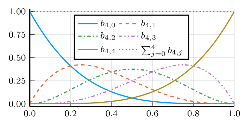
Figure 4: Bernstein basis polynomials of degree 4, along with their sum.

The following result shows how $p$ can be bounded by its Bernstein coefficients [2].

Theorem 1

Let $p_{\min}$ and $p_{\max}$ be the minimum and maximum values of $p(t)$, for $t\in[0,1]$. Then $p$ is bounded in $[0,1]$ by

$$\min\{\beta_{j}\}_{j=0}^{n_{p}}\leq p_{\min}\quad\text{and}\quad\max\{\beta_{j}\}_{j=0}^{n_{p}}\geq p_{\max}.$$ (22)

Moreover, the bounds are tight in the following cases:

$$\min\{\beta_{j}\}_{j=0}^{n_{p}} =\beta_{0} \iff \min\{\beta_{j}\}_{j=0}^{n_{p}}=p_{\min},$$ (23)

$$\max\{\beta_{j}\}_{j=0}^{n_{p}} =\beta_{n} \iff \max\{\beta_{j}\}_{j=0}^{n_{p}}=p_{\max},$$ (24)

$$\max\{\beta_{j}\}_{j=0}^{n_{p}} =\beta_{0} \iff \max\{\beta_{j}\}_{j=0}^{n_{p}}=p_{\max},$$ (25)

$$\min\{\beta_{j}\}_{j=0}^{n_{p}} =\beta_{n} \iff \min\{\beta_{j}\}_{j=0}^{n_{p}}=p_{\min}.$$ (26)

It has also been shown that the Bernstein coefficients can be computed from the monomial coefficients [2] by

$$\beta_{j}=\sum_{k=0}^{j}\alpha_{k}\left.\binom{j}{k}\middle/\binom{n_{p}}{k}\right..$$ (27)

This change of basis can be written in matrix form

$$\beta=B\alpha,$$ (28)

where $\beta$ and $\alpha$ are ordered column vectors of $\{\beta_{j}\}_{j=0}^{n_{p}}$ and $\{\alpha_{k}\}_{k=0}^{n_{p}}$ respectively, and $B$ is a lower triangular matrix.

III-B Bounds on Interpolating Polynomials

Let $\widetilde{y}:[{-}1,1]\times\mathbb{R}^{n_{p}+1}\rightarrow\mathbb{R}$, $(\tau,y)\mapsto\widetilde{y}(\tau;y)$ be the Lagrange interpolating polynomial at points $\{\tau^{y}_{j}\}_{j=0}^{n_{p}}$ with coefficients $y$. The Bernstein coefficients of $\widetilde{y}(\cdot;y)$ can be obtained by

$$\beta=Cy,\quad C=BV^{-1},$$ (29)

where $V$ is the Vandermonde matrix for the linearly scaled points $\{0.5\tau^{y}_{j}+0.5\}_{j=0}^{n_{p}}$. Hence, for the scalars $y_{\ell}<y_{u}$,

$$y_{\ell}\leq Cy\leq y_{u}\implies y_{\ell}\leq\widetilde{y}(\tau;y)\leq y_{u},\,\forall\tau\in[-1,1].$$ (30)

This approach is used to enforce the inequality constraints of (P) on the discretized dynamic variables, thus satisfying

$$\widetilde{x}(\tau;x_{i})\in\mathbb{X},\quad\widetilde{u}(\tau;u_{u})\in\mathbb{U},\quad\forall\tau\in[-1,1],$$ (31)

for every sub-interval $i\in\{1,2,...,n_{h}\}$.

III-C Tight Bounds on Finite Sub-Intervals

One may wonder if $\widetilde{x}$ and $\widetilde{u}$ can always be tightly bounded, given a sufficiently flexible sub-interval. For the case of monotonic polynomials, the following result shows they can be partitioned into a finite number of tightly bounded polynomials.

Theorem 2

Let $p$ be a univariate polynomial of degree at most $n_{p}$ that is monotonic on a finite interval $[t_{a},t_{b}]$. There exists a finite set of partitions of $[t_{a},t_{b}]$, such that $p$ is tightly bounded in every partition.

Proof:

Without loss of generality, we consider the interval $t_{a}=0$ and $t_{b}=1$, and attempt to find a sub-interval $[0,s]$, with $0<s\leq 1$, on which there are tight bounds for $p$. Let the monomial coefficients of $p$ be $\{\alpha_{k}\}_{k=0}^{n_{p}}$. Let $p_{s}$ be a linearly scaled version of $p$, such that $p_{s}(0)=p(0)$ and $p_{s}(1)=p(s)$. The monomial coefficients of $p_{s}$ are $\{\alpha_{k}s^{k}\}_{k=0}^{n_{p}}$, and let $\{\beta_{j}\}_{j=0}^{n_{p}}$ be the Bernstein coefficients of $p_{s}$.

For the case where $p$ is non-decreasing in $[0,1]$, $p_{s}(0)=\beta_{0}$ and $p_{s}(1)=\beta_{n_{p}}$, and the conditions for tight bounds (23) and (24) require that

$$\beta_{0}\leq\beta_{j}\leq\beta_{n_{p}},$$ (32)

for $j\in\{1,2,...,n_{p}-1\}$. Equivalently, in the monomial basis,

$$\alpha_{0}\leq\sum_{k=0}^{n_{p}}B_{j,k}\alpha_{k}s^{k}\leq\sum_{k=0}^{n_{p}}\alpha_{k}s^{k}.$$ (33)

Since $B_{j,0}=1$, $\alpha_{0}$ can be subtracted, leaving

$$0\leq\sum_{k=1}^{n_{p}}B_{j,k}\alpha_{k}s^{k}\leq\sum_{k=1}^{n_{p}}\alpha_{k}s^{k}.$$ (34)

In the case that all $\{\alpha_{k}\}_{k=1}^{n_{p}}=0$, (34) is trivially satisfied. Otherwise, given that $\{s^{k}\}_{k=1}^{n_{p}}$ is a geometric sequence, for a sufficiently small $s$, the first term of the sums for which $\{\alpha_{k}\}_{k=1}^{n_{p}}$ is non-zero, becomes sufficiently large, so that:

• The left sum becomes non-negative, since the first non-zero element of $\{\alpha_{k}\}_{k=1}^{n_{p}}$ is positive for a non-decreasing, non-constant polynomial;

• The left sum becomes less or equal to the right sum, since all the elements of $B_{j,k}$, for $j\in\{1,2,...,n_{p}-1\},k\in\{1,2,...,n_{p}\}$, are strictly less than 1.

A similar argument can be made for the case where $p$ is non-increasing on $[t_{a},t_{b}]$, using the tight bound conditions (25) and (26). ∎

In practice, Theorem 2 suggests that a sufficient number of flexible sub-intervals must be chosen so as to tightly bound $\widetilde{x}$ and $\widetilde{u}$. The monotonicity assumption is rather mild, since most functions can be approximated by piecewise-monotonic piecewise polynomials. Moreover, it has been shown that monotonic polynomials can approximate monotonic functions with a similar rate of convergence as in the unconstrained case [9].

IV Example Problem

IV-A Constrained Cart-Pole Swing-Up

The problem of optimally swinging up a cart-pole system has been described in [10, Sect. 6], with parameters given in [10, App. E.1]. This optimal control problem has a single input $\boldsymbol{u}$, for the force acting on the cart, and four states $\boldsymbol{x}:=[\boldsymbol{q}_{1},\boldsymbol{q}_{2},\dot{\boldsymbol{q}}_{1},\dot{\boldsymbol{q}}_{2}]^{\top}$, where $\boldsymbol{q}_{1}$ is the position of the cart and $\boldsymbol{q}_{2}$ is angle of the pole. Because none of the inequality constraints are active at the solution to the original problem, we consider the case where the cart’s position is further constrained to satisfy

$$0\leq\boldsymbol{q}_{1}(t)\leq 1,\quad\forall t\in[t_{0},t_{f}].$$ (35)

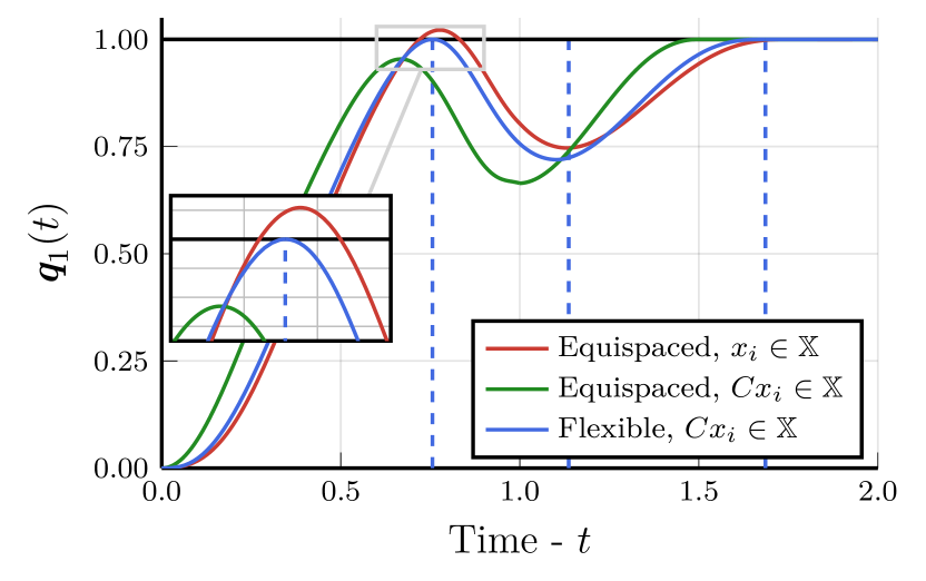
Figure 5: Trajectories of the cart’s position for the three discretizations, with dashed lines indicating the flexible sub-intervals.

Approximate solutions to the constrained cart-pole swing-up problem were obtained for the following discretization approaches:

1. Equispaced sub-intervals, with inequality constraints enforced at the interpolation points, as per (18);

2. Equispaced sub-intervals, with inequality constraints enforced on the Bernstein coefficients, as per (30);

3. Flexible sub-intervals, with inequality constraints enforced on the Bernstein coefficients, as per (30).

Figure 5 shows approximate solutions for $\boldsymbol{q}_{1}$ using the three approaches, with LGR collocation degree $n=7$ and $n_{h}=4$ sub-intervals, all with flexibility $\phi=50\%$. As the figure shows, approach (a) violates the inequality constraint, whereas there are no violations with approaches (b) and (c), as expected. It can also be seen how approach (b) is rather conservative, in contrast to approach (c). In this example, as with many others, there is a cost incentive to operate near the constraints.

IV-B Criteria for Approximate Solutions

To assess an approximate solution $(x^{*},u^{*})$ to the constrained cart-pole problem, the following criteria are considered.

IV-B1 Cost

As in [10], the cost is simply

$$\int_{t_{0}}^{t_{f}}u^{*}(t)^{2}\textrm{d}t.$$ (36)

IV-B2 Inequality Constraint Violation

We define the violation function for a scalar-valued trajectory $y:[t_{0},t_{f}]\rightarrow\mathbb{R}$ with lower and upper constraints $y_{\ell}$ and $y_{u}$ respectively, as

$$v(t;y,y_{\ell},y_{u}):=\begin{cases}y_{\ell}-y(t),&\text{if $y(t)<y_{\ell}$}\\ y(t)-y_{u},&\text{if $y(t)>y_{u}$}\\ 0,&\text{otherwise.}\end{cases}$$ (37)

The total inequality constraint violation is defined as the sum of violation norms for the input and the four states, i.e.

$$\|v(\cdot;u^{*},u_{\ell},u_{u})\|_{2}+\sum_{k=1}^{4}\|v(\cdot;x^{*}_{k},x_{\ell,k},x_{u,k})\|_{2},$$ (38)

where the 2-norm $\|f\|_{2}:=\sqrt{\int_{t_{0}}^{t_{f}}|f(t)|^{2}\textrm{d}t}$, for $f:[t_{0},t_{f}]\rightarrow\mathbb{R}$. The input constraints are given by $u_{\ell}$ and $u_{u}$, and the $k^{\text{th}}$ state constraints are given by $x_{\ell,k}$ and $x_{u,k}$.

IV-B3 Dynamics Error

This is defined as the average 2-norm of the violation of the four dynamic equations, i.e.

$$\frac{1}{4}\sum_{k=1}^{4}\|r_{k}(\dot{x}^{*}(\cdot),x^{*}(\cdot),u^{*}(\cdot),\cdot)\|_{2}.$$ (39)

IV-C Convergence

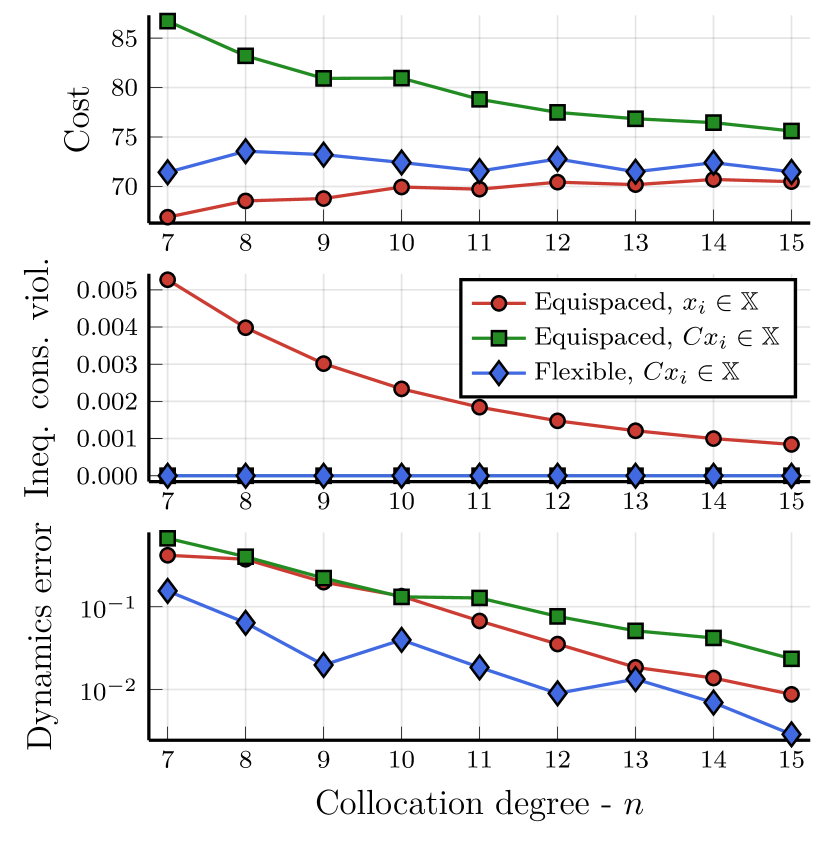
Figure 6: Assessment of numerical solutions of the three approaches, for a range of collocation degrees.

Figure 6 shows a comparison of approaches (a), (b) and (c), for each of the three criteria. Even with higher polynomial degrees, approach (a) continues to violate the inequality constraints. With this violation, approach (a) is able to obtain a smaller cost, in comparison with (b) and (c). Approach (b) reports a significantly greater cost, due to the conservative Bernstein bounds. The sub-interval flexibility allows approach (c) to eliminate the conservatism of the Bernstein bounds and obtain a smaller cost, in comparison with approach (b).

It should be noted, however, that for lower $n$, the solutions exhibit a higher dynamics error, which, in practice, may demerit the large differences in cost.

IV-D Sub-Interval Flexibility

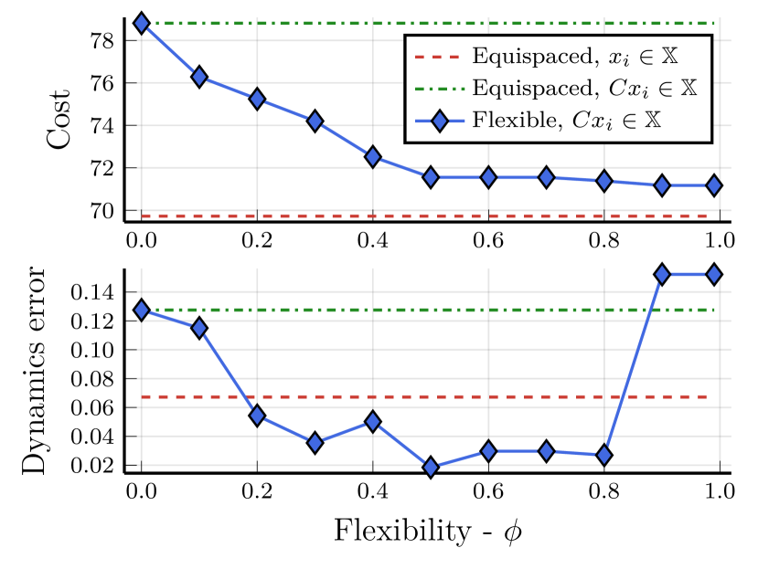
Figure 7: Cost and dynamics error for a range of flexibility parameters. Dashed lines compare the solutions of approaches (a) and (b).

Figure 7 shows the impact of the flexibility parameter on the cost and dynamic error. As expected, in the special case of $\phi=0\%$, approach (c) is indistinguishable from approach (b). For $n=7$, a flexibility of $\phi=50\%$ allows for a significant decrease in cost, without compromising on the dynamics error. Ample flexibility may create large sub-intervals, resulting in locally less dense discretizations, thus increasing the overall dynamics error of the solution.

V Conclusion

A pseudo-spectral method for DOPs was presented which not only rigorously enforces inequality constraints, but also allows for tight polynomial bounds to be achieved via flexible sub-intervals. A theoretical result on obtaining tight polynomial bounds with a finite number of sub-intervals was also presented. Enforcing the DOP dynamics on flexible sub-intervals results in a non-convex optimization problem. In some applications with linear dynamics, the non-convexity of the proposed approach may be a drawback, in comparison with SOS or fixed sub-interval approaches. An in-depth study of this non-convexity, as well as potential convexification techniques are worthy of further research.

Appendix

V-A Sine Approximation Problem

The function approximation problem in Section I is defined as finding $\boldsymbol{y}:[0,1]\rightarrow\mathbb{R}$ that minimizes

$$\int_{0}^{1}(\sin(2\pi t)-\boldsymbol{y}(t))^{2}\textrm{d}t,$$ (40)

subject to the inequality constraints $-1\leq\boldsymbol{y}(t)\leq 1,\forall t\in[0,1]$. In the case of flexible sub-intervals, (40) is approximated by

$$\sum_{i=1}^{3}\frac{\stackrel{{\scriptstyle\leftrightarrow}}{{t}}_{i}-\stackrel{{\scriptstyle\leftrightarrow}}{{t}}_{i-1}}{2}\sum_{q=0}^{n_{q}}w_{q}\big{(}\sin(2\pi\gamma(\tau_{q},\stackrel{{\scriptstyle\leftrightarrow}}{{t}}_{i-1},\stackrel{{\scriptstyle\leftrightarrow}}{{t}}_{i}))-\widetilde{y}(\tau_{q};y_{i})\big{)}^{2},$$ (41)

where $\{\tau_{q}\}_{q=0}^{n_{q}}$ and $\{w_{q}\}_{q=0}^{n_{q}}$ are the Legendre-Gauss-Lobatto (LGL) quadrature points and weights, respectively. And $\widetilde{y}$ is an interpolating polynomial using $n_{p}+1$ LGL points. It is chosen that $n_{q}=n_{p}+2$.

V-B Numerical Integrations

The numerical integration in (36), (38), and (39) was performed using the software package QuadGK.jl (version 2.9.4, available from https://github.com/JuliaMath/QuadGK.jl) with the default options.

References

- [1] G. Szegő, Orthogonal Polynomials, vol. 23 of Colloquium Publications. American Mathematical Society, Dec. 1939.
- [2] G. Cargo and O. Shisha, “The Bernstein form of a polynomial,” Journal of Research of the National Bureau of Standards Section B Mathematics and Mathematical Physics, vol. 70B, pp. 79–81, Jan. 1966.
- [3] N. Koeppen, I. M. Ross, L. C. Wilcox, and R. J. Proulx, “Fast Mesh Refinement in Pseudospectral Optimal Control,” Journal of Guidance, Control, and Dynamics, vol. 42, no. 4, pp. 711–722, 2019.
- [4] V. Cichella, I. Kaminer, C. Walton, N. Hovakimyan, and A. M. Pascoal, “Optimal Multivehicle Motion Planning Using Bernstein Approximants,” IEEE Transactions on Automatic Control, vol. 66, pp. 1453–1467, Apr. 2021.
- [5] J. P. Allamaa, P. Patrinos, H. Van Der Auweraer, and T. D. Son, “Safety Envelope for Orthogonal Collocation Methods in Embedded Optimal Control,” in 2023 European Control Conference (ECC), pp. 1–7, June 2023.
- [6] J. P. Allamaa, P. Patrinos, T. Ohtsuka, and T. D. Son, “Real-time MPC with Control Barrier Functions for Autonomous Driving using Safety Enhanced Collocation,” Jan. 2024. arXiv:2401.06648 [cs, eess, math].
- [7] I. M. Ross and F. Fahroo, “Pseudospectral Knotting Methods for Solving Nonsmooth Optimal Control Problems,” Journal of Guidance, Control, and Dynamics, vol. 27, no. 3, pp. 397–405, 2004.
- [8] L. Nita, E. M. G. Vila, M. A. Zagorowska, E. C. Kerrigan, Y. Nie, I. McInerney, and P. Falugi, “Fast and accurate method for computing non-smooth solutions to constrained control problems,” in 2022 European Control Conference (ECC), pp. 1049–1054, July 2022.
- [9] R. A. De Vore, “Monotone Approximation by Polynomials,” SIAM Journal on Mathematical Analysis, vol. 8, pp. 906–921, Oct. 1977.
- [10] M. Kelly, “An Introduction to Trajectory Optimization: How to Do Your Own Direct Collocation,” SIAM Review, vol. 59, pp. 849–904, Jan. 2017.