Precision timing of eclipsing binaries from TESS full frame images. Method and performance

Abstract

Several hundreds of thousands of eclipsing binaries (EBs) are expected to be detected in the Transiting Exoplanet Survey Satellite (TESS) full frame images (FFIs). This represents a significant increase in the number of EBs available for eclipse timing variation studies. In this paper, we investigate the feasibility of performing precise eclipse timing of TESS EBs using the FFIs. To this end, we developed a fast, automated method and applied it to a sample of $\sim$100 EBs selected from the Villanova TESS EB catalog. Our timing analysis resulted in the detection of ten new triple candidates with outer periods shorter than $\sim$1300 d. For five of them, we were able to constrain the outer orbit by analyzing independently the short-cadence (SC) and FFI data and to derive the minimum mass of the third body with a precision better than 4 per cent for SC and 12 per cent for FFI data. We then compared the results obtained from the two datasets and found that using the FFI data leads to (1) a degradation of both the accuracy and precision of the tertiary mass determination for the tightest EBs and (2) an overall underestimation of the third component’s mass. However, we stress that our main conclusions on the nature of the detected signals do not depend on which dataset is used. This confirms the great potential of TESS FFIs, which will allow us to search for rare objects such as substellar circumbinary companions and compact triple stellar systems.

1 Introduction

Since its launch in 2018, the Transiting Exoplanet Survey Satellite (TESS; Ricker et al. 2015) has been surveying the majority of the sky, resulting in the detection of thousands of exoplanet candidates (Guerrero et al., 2021), solar-like oscillators (Hatt et al., 2023), and eclipsing binaries (EBs; Prša et al. 2022) among $\sim$200,000 pre-selected stars observed in 2-min short-cadence (SC) mode during the 2-yr prime mission (Sectors 1–26). In addition, TESS acquired images of each observing sector, referred to as full frame images, or FFIs, every 30 minutes. Over a billion stars were observed in this mode, therefore providing a huge data-mining archive for large ensemble studies, such as galactic archeology (Silva Aguirre et al., 2020). During the first extended mission (Sectors 27–55), the FFI cadence was reduced to 10 minutes, and a new 20-s ultra-short-cadence (USC) mode was implemented. TESS is currently in its second extended mission (Sectors 56–69), and observes 2000 stars at 20-s cadence and 12,000 stars at 2-min cadence per sector, while FFIs are now retrieved at a shorter 200-s cadence.

Based on the SC data collected during the prime mission, Prša et al. (2022) produced a catalog of 4584 EBs detected among the $\sim$200,000 pre-selected TESS targets. EBs are among the most fundamental calibrators of stellar physics. In particular, it is possible to measure the masses and radii of each component of a double-lined (SB2) eclipsing binary with an exquisite precision, better than $\sim$1–3 per cent, and to derive its age without resorting to more advanced stellar modeling (Hełminiak et al., 2021). For example, EBs hosting oscillating red giants are valuable benchmarks to test the ability of ensemble asteroseismology to reproduce the stellar properties (Benbakoura et al., 2021) and to calibrate model parameters, such as the mixing-length parameter (Li et al., 2018). EBs have also proven to be powerful tools for distance determinations of Local Group galaxies (Pietrzyński et al., 2019). Finally, EBs that belong to multiple stellar systems are ideal to study the orbital architecture and dynamics (Marcadon et al., 2020; Moharana et al., 2023).

Stellar multiplicity is an ubiquitous outcome of star formation. Indeed, almost half of solar-type stars are in binaries or multiple systems ($\sim$35 and 10 per cent of the total population, respectively), as reported by Raghavan et al. (2010) from a survey of stellar multiplicity in the solar neighborhood. The occurrence rate of close binaries with tertiary companions ($\sim$20 per cent of the EB population) was confirmed by Conroy et al. (2014), who analyzed a sample of 1279 Kepler eclipsing binaries using the so-called eclipse timing variation method. Eclipse timing variations (ETVs) are generally attributed to the light-travel time effect (LTTE; Mayer 1990), also known as the Rømer delay, caused by the presence of a circumbinary third body. The ETV method is therefore particularly suitable for identifying compact hierarchical triples (CHTs; Borkovits 2022) and substellar circumbinary companions (Wolf et al., 2016, 2018, 2021) from both space-based and ground-based surveys. Increasing the detection of these objects will considerably improve our knowledge of the formation of stars and planets in binaries or multiple stellar systems (Marzari & Thebault, 2019; Tokovinin, 2021). On the one hand, there is a clear deficit of CHTs with binary periods $\lesssim\,$1 d and outer periods $\lesssim\,$200 d (Borkovits et al., 2016). On the other hand, only a dozen or so circumbinary planets are presently known (Marzari & Thebault, 2019).

The TESS FFIs contain hundreds of thousands of EBs (Kruse et al., 2021), among which several thousand are expected to be located in the continuous viewing zones (CVZs). As they benefit from long-duration observations, CVZ EBs are promising targets for finding CHTs and circumbinary planets using the ETV method. Given the expected large number of CVZ EBs to be detected in the FFIs, it is necessary to use a fast, automated method for performing precise eclipse timing. In this paper, the first in a series, we aim to validate the light-curve extraction from the TESS FFIs using the calibrated 2-min cadence light curves, and to demonstrate the potential of our method for recovering the ETV signal of a third body using the FFIs. The paper is organized as follows. We describe our target selection in Section 2, as well as the TESS observations and data reduction. In Section 3, we present our method to measure precise eclipse times and to determine third-body solutions from ETVs. In Section 4, we discuss the results obtained for five EBs with a firm third-body detection, focusing on the comparison between SC and FFI results. Finally, in Section 5, we summarize the conclusions of this work and outline future prospects.

2 Targets and data

2.1 Target selection

To select TESS EB targets suitable for long-duration ETV surveys from both the SC and FFI datasets, we made use of the Villanova TESS EB catalog (Prša et al., 2022), which lists 4584 EB targets observed in SC mode during the prime mission. Among them, we identified $\sim$400 targets in the CVZs, that is, with an ecliptic latitude $|\beta|>78^{\circ}$. As illustrated in Figure 2 of Prša et al. (2022), the catalog contains a variety of systems, from contact and ellipsoidal binaries with periods as short as 0.1 d to wide detached binaries with periods of tens of days. For this reason, Prša et al. (2022) adopted the morphology coefficient defined by Matijevič et al. (2012) to describe the “detachedness” of a binary. This parameter continuously varies between 0 and 1, where 0 corresponds to the widest detached binaries and 1 to contact binaries and ellipsoidal variables. The timing method described in this paper was initially developed for the ETV analysis of detached and semi-detached EBs, that is, EBs with a morphology coefficient less than $\sim$0.7 (Marcadon et al., 2020; Moharana et al., 2024).

As a part of the selection process, we applied our timing procedure to the full set of $\sim$400 CVZ targets previously identified in the Villanova TESS EB catalog. We also performed a visual inspection of the light curves to identify detached and semi-detached EBs in the sample. Thus, from our original sample, we were able to measure the eclipse times of $\sim$100 detached and semi-detached EBs with a period shorter than 27 d, i.e. the observing duration of one TESS sector. Finally, we inspected the resulting $O-C$ (observed minus calculated times) curves of these $\sim$100 EBs, and we found that 10 of them show ETV signals with periods less than $\sim$1300 d (corresponding to the maximum time span of the observations used in this work). It is worth noting that the third-body occurrence rate in our sample, $\sim$10 per cent, is consistent with that found by Conroy et al. (2014) for a range of outer periods up to $\sim$1400 d. For five of our ten newly identified triple systems, the good coverage of the outer orbit with observations in SC mode allowed us to make a direct comparison with the results obtained using the FFI data. These five systems were observed in Sectors 14–26, 40–41, and 47–60, implying a coverage of their outer orbits of at least 60 per cent. They are listed in Table 1.

Table 1: Properties of the detected systems taken from the Villanova TESS EB catalog. The five systems investigated in this work are marked by an asterisk.

TIC	$T_{0}$	$P_{1}$	Morph.	$T_{\rm mag}$
	BJD$-245\,7000$	(d)
38699825	$1410.972\,4(40)$	$2.084\,644(11)$	0.592	8.296
141685465	$1416.199\,5(14)$	$7.807\,423(97)$	0.220	11.3742
150361911	$1545.543\,040(99)$	$2.493\,8523(28)$	0.461	12.1631
219900027*	$1683.750\,363(15)$	$0.515\,26471(79)$	0.684	11.2024
229771234*	$1931.061\,6(66)$	$0.820\,95849(30)$	0.722	10.7665
259006185*	$1901.860\,148(45)$	$1.939\,6542(16)$	0.346	9.11642
278956474a	$1327.960\,81(26)$	$5.488\,050(12)$	0.314	12.9637
356896561*	$1685.409\,425(11)$	$2.253\,35087(11)$	0.455	9.1494
373915220	$1329.027\,38(34)$	$6.470\,6807(19)$	0.149	11.4541
424461577*	$1712.102\,37(17)$	$0.744\,82334(12)$	0.654	10.1535

2.2 Short-cadence data

We first analyzed the SC data collected by TESS for our initial sample of $\sim$400 CVZ targets. These data were generated by the TESS Science Processing Operations Center (SPOC; Jenkins et al. 2016) and made available on the Mikulski Archive for Space Telescopes (MAST). We employed the astroquery package (Ginsburg et al., 2019) to download the SC light curves of our targets from Sectors 1 to 60. In our analysis, we chose to use the Pre-search Data Conditioning Simple Aperture Photometry (PDCSAP) light curves (Smith et al., 2012; Stumpe et al., 2012, 2014), which have been corrected for instrumental effects and contamination by nearby stars. Then, we normalized the light curves by dividing by the median flux value of each sector.

2.3 Full-frame image data

For all of our CVZ targets, we also extracted FFI light curves from all available sectors using the eleanor package (Feinstein et al., 2019) with the default settings. We briefly describe the main steps of the light-curve extraction with eleanor. First, we download a $31\times 31$ pixel postcard of the FFIs centered on each target using the TESScut tool (Brasseur et al., 2019) called by eleanor. A $13\times 13$ target pixel file (TPF) is then extracted from each postcard, and aperture photometry is performed on the TPF. We used a fixed aperture of $3\times 3$ pixels from the eleanor default library, which yields the lowest point-to-point scatter for the range of magnitudes of our targets (Nardiello, 2020). Eleanor provides three different types of light curves from aperture photometry: raw light curves, corrected light curves, and principal component analysis (PCA) light curves. For our analysis, we used the corrected light curves, where signals correlated to pixel position, measured background and time have been removed, and we excluded all flux measurements with nonzero quality flags. Finally, the FFI light curves were normalized in the same way as the SC light curves. The SC and FFI light curves of the five investigated targets are shown in Figure 1 and Appendix A.

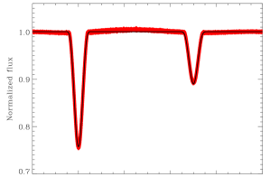
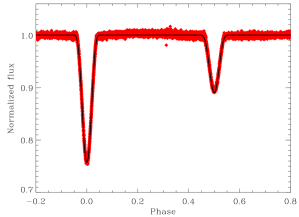
Figure 1: The TESS SC (top) and FFI (bottom) light curves of TIC 356896561 (presented here is Sector 57). Red symbols denote the observations while the solid line corresponds to the best-fit model of the SC light curve determined using the procedure described in Section 3.2.

3 Method and analysis

3.1 Bayesian inference method

Recently, Moharana et al. (2024) published the first results of the Solaris ground-based photometric survey, which led to the detection of a new CHT candidate, GSC 08814-01026, using the ETV method. The present section aims to describe the Bayesian formalism adopted in this work, as well as in Moharana et al. (2024), for the derivation of the times of minima.

According to Bayes’ theorem, the posterior probability density of the parameters $\Theta$ given data $D$ is stated as

$$P(\Theta|D)=\frac{P(\Theta)\,P(D|\Theta)}{P(D)},$$ (1)

where $P(\Theta)$ is the prior probability density of the parameters, $P(D)$ is the global normalization likelihood and $P(D|\Theta)$ is the likelihood ${\cal L}$ of the data given the parameters. Here, we define the likelihood ${\cal L}=\exp(-\chi^{2}/2)$ with

$$\chi^{2}=\sum^{N}_{i=1}\,\left(\frac{D_{i}-M_{i}(\Theta)}{\sigma_{i}}\right)^{2},$$ (2)

where $N$ denotes the number of observed data points, $\sigma_{i}$ refers to the associated uncertainties, and $M(\Theta)$ is the model function used to fit the data (see Sections 3.2 and 3.3). The sampling of the posterior probabilities can be done by exploring the parameter space using Markov Chain Monte Carlo (MCMC) methods, such as the Metropolis–Hastings algorithm (MH; Metropolis et al. 1953; Hastings 1970). Our implementation of the MH algorithm works as follows. We set a chain of N points with starting points $\Theta^{t}$ taken randomly from appropriate distributions. The new set of parameters $\Theta^{t^{\prime}}$ is computed using a random walk as

$$\Theta^{t^{\prime}}=\Theta^{t}+\alpha_{\rm rate}\,\Delta\Theta,$$ (3)

where $\Delta\Theta$ is given by a multivariate normal distribution with independent parameters and $\alpha_{\rm rate}$ is an adjustable parameter that is reduced by a factor of two until the rate of acceptance of the new set exceeds 25 per cent, marking the end of the burn-in phase (first 10 per cent of the chain). We assume here that either set has the same probability, i.e. $P(\Theta^{t})=P(\Theta^{t^{\prime}})$. From Equation (1), we can then define the ratio

$$r=\frac{P(\Theta^{t^{\prime}}|D)}{P(\Theta^{t}|D)}=\frac{P(D|\Theta^{t^{\prime}})}{P(D|\Theta^{t})},$$ (4)

which is equivalent to the ratio of the likelihoods, known as the Bayes factor. The acceptance probability of the new set, $\Theta^{t^{\prime}}$, is computed as

$$\alpha(\Theta^{t},\Theta^{t^{\prime}})={\rm min}\,(1,r)={\rm min}\left(1,\frac{P(D|\Theta^{t^{\prime}})}{P(D|\Theta^{t})}\right).$$ (5)

The new values of the parameters are accepted if $\beta\leq\alpha$, where $\beta$ is a random number drawn from a uniform distribution over the interval $[0,1]$, and rejected otherwise. We derive the posterior probability distribution of each parameter from the Markov chain after rejecting the initial burn-in phase. For all parameters, we compute the median and the credible intervals at 16 per cent and 84 per cent, corresponding to a 1$\sigma$ interval for a normal distribution. The advantage of this percentile definition over the mode (maximum of the posterior distribution) or the mean (average of the distribution) is that it is conservative with respect to any change of variable over these parameters (see Section 4.1).

3.2 Determination of times of minima

In order to measure the times of eclipse minima, we approximated the phased light curves of our targets using the phenomenological model of Mikulášek (2015), which analytically describes the eclipse profile as

$$f(t_{i},\Theta)=\alpha_{0}+\sum^{n_{e}}_{k=1}\alpha_{k}\,\psi(t_{i},T_{k},d_{k},\Gamma_{k},C_{k}),$$ (6)

where $\alpha_{0}$ is the flux zero-point shift, $\alpha_{k}$ is a scaling coefficient of the eclipse profile function $\psi$, and $n_{e}$ is the number of eclipses during one cycle. Among the seven different model functions proposed by Mikulášek (2015), we chose the form:

$$\psi(t_{i},T,d,\Gamma,C)=\Bigg{\{}1+C\bigg{(}\frac{t_{i}-T}{d}\bigg{)}^{2}\Bigg{\}}\Bigg{\{}1-\bigg{\{}1-\exp\bigg{[}1-\cosh\bigg{(}\frac{t_{i}-T}{d}\bigg{)}\bigg{]}\bigg{\}}^{\Gamma}\Bigg{\}},$$ (7)

which is suitable for detached and semi-detached EBs (see Marcadon et al. 2020 and Moharana et al. 2024 who used a simpler form of $\psi$). Here, $T$, $d$, $\Gamma$, and $C$ are the time of minimum, the eclipse width, the kurtosis, and the scaling parameter, respectively. For each individual eclipse, the time of minimum is estimated as

$$\begin{split}T_{k}&=T_{0,k}+PE+\Delta_{k}\\ &=T_{0,k}+P\times{\rm round}\bigg{(}\frac{t_{i}-T_{0,k}}{P}\bigg{)}+\Delta_{k},\end{split}$$ (8)

where $T_{0,k}$, $P$, $E$, and $\Delta_{k}$ are the reference time of eclipse, the orbital period, the epoch, and the $O-C$ time difference, respectively. Each light curve is thus described by $\Theta=(\alpha_{0},\alpha_{k},T_{0,k},d_{k},\Gamma_{k},C_{k},\Delta_{k},P)$, where $\Delta_{k}$ is a vector with size equal to the number of cycles.

In the first step of the modeling process, we applied our MCMC procedure to the PDCSAP light curve of each target assuming that the eclipses are strictly periodic (i.e., $\Delta_{k}=0$ for each eclipse). For each target, we generated ten chains of $10^{5}$ points each as described in Section 3.1. From each chain, we obtained a set of parameters that best fits the light curve of a single sector (randomly selected among the available sectors). We then computed the chi-squared ($\chi^{2}$) for all sets of parameters as defined in Equation (2) and adopted as reference the set with the smaller value of $\chi^{2}/N$ among the ten MCMC chains. In Figure 1 and Appendix A, we compare our best-fit models, derived from a single sector, to the SC and FFI light curves of the five investigated systems. In the second step, we used our MCMC algorithm to determine the times of minima from both the PDCSAP and FFI light curves. Here, we generated a chain of $10^{4}$ points for each available SC sector. During the fitting, we left $\Delta_{k}$ as a free parameter and we fixed the other parameters to their best-fit values obtained in the initial fit. We then calculated the times of minima from the best-fit values of the parameter $\Delta_{k}$ using Equation (8). We repeated this step for all FFI sectors. Finally, the measured times of all eclipses occurring during data gaps were removed, an iterative sigma-clipping technique was applied to the remaining eclipse times, and the error bars were properly rescaled (see Section 3.3). For the five systems studied here, we provide the times of minima derived from both the PDCSAP and FFI light curves in Table 2.

Table 2: Measured times of minima for the systems investigated in this work.

TIC	Time	Cycle	1$\sigma$ error	$\Delta_{\rm obs}$	${\rm O}-{\rm C}$	Obs. mode
	BJD$-245\,7000$	no.	(d)	(s)	(s)
356896561	$1684.282\,68$	$-$532.5	$0.000\,27$	61.7	29.0	SC
356896561	$1685.408\,82$	$-$532.0	$0.000\,13$	14.9	$-$18.3	SC
356896561	$1686.535\,95$	$-$531.5	$0.000\,30$	53.7	19.9	SC
356896561	$1687.662\,17$	$-$531.0	$0.000\,13$	14.2	$-$20.2	SC
356896561	$1688.789\,19$	$-$530.5	$0.000\,26$	43.3	8.4	SC
356896561	$1689.915\,52$	$-$530.0	$0.000\,13$	13.4	$-$22.1	SC
356896561	$1691.042\,49$	$-$529.5	$0.000\,27$	38.1	2.1	SC
356896561	$1697.802\,65$	$-$526.5	$0.000\,27$	45.5	6.4	SC
356896561	$1698.929\,08$	$-$526.0	$0.000\,13$	23.9	$-$15.7	SC
356896561	$1700.056\,12$	$-$525.5	$0.000\,29$	54.5	14.4	SC
356896561	$1701.182\,45$	$-$525.0	$0.000\,13$	24.7	$-$15.9	SC

3.3 Eclipse timing variation analysis

A common method to search for ETVs is to construct an $O-C$ diagram showing the difference between the observed and calculated times of minima, i.e.

$$\Delta_{\rm obs}=T_{\rm o}(E)-T_{\rm c}(E)=T_{\rm o}(E)-T_{0}-PE,$$ (9)

where $T_{\rm o}(E)$ and $T_{\rm c}(E)$ refer to the observed and calculated times of minima at epoch $E$, respectively. Here, the values of $T_{0}$ and $P$ are taken from the best-fit light-curve models obtained in Section 3.2. The resulting $O-C$ diagrams of the five systems investigated in this work are shown in Figure 2 and Appendix B.

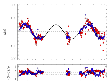
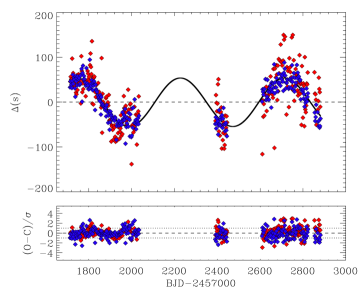
Figure 2: ETVs for TIC 356896561 determined from the SC (top) and FFI (bottom) light curves. Blue and red diamonds refer to the primary and secondary eclipse times, respectively, derived as explained in Section 3.2. The best-fit ETV solution is overplotted as a solid line. Fitting residuals are shown in lower panels.

As mentioned previously, ETVs can be attributed to the LTTE caused by the gravitational influence of a third body orbiting an EB. There are, however, various other mechanisms capable of inducing ETVs in an EB, such as the apsidal motion and dynamical perturbation effects (see e.g. Borkovits et al. 2015, for a review). Apsidal motion consists in the rotation of the line of apsides in an eccentric binary and has an anticorrelated effect for primary and secondary minima variations. In the following, apsidal motion is precluded as the five EBs presented here are nearly circular. Furthermore, in the presence of a third body, the EB undergoes a number of dynamical perturbations, implying that its orbit is no longer Keplerian. The dynamical perturbations affect all the orbital elements of the EB and, thus, the occurrence times of the eclipses. Borkovits et al. (2016) showed that the amplitude of the dynamical contribution for a circular EB orbit can be written as

$${\mathcal{A}}_{\rm dyn}=\frac{1}{2\pi}\frac{M_{\rm B}}{M_{\rm A}+M_{\rm B}}\,\frac{P_{1}^{2}}{P_{2}}\big{(}1-e_{2}^{2}\big{)}^{-3/2},$$ (10)

where $M_{A}$ and $M_{B}$ are the masses of the eclipsing pair and the third body, respectively, and $e_{2}$ is the eccentricity. The subscript ‘1’ refers to the inner orbit, i.e. the eclipsing pair A, while the subscript ‘2’ refers to the relative orbit between the eclipsing pair A and the third body B, hereafter referred to as the AB system. Equation (10) attests that the dynamical ETV contribution is expected to be more important for the systems in our sample that have the smallest $P_{2}/P_{1}$ ratio (TIC 259006185 and TIC 356896561). However, in the present study, we neglect the possible contribution of the dynamical perturbations. We thus modeled the ETVs in the mathematical form of LTTE (Borkovits et al., 2015, 2016):

$$\Delta_{\rm mod}=c_{0}+c_{1}E-\frac{a_{\rm A}\sin i_{2}}{c}\,\frac{\big{(}1-e_{2}^{2}\big{)}\sin(\upsilon_{2}+\omega_{2})}{1+e_{2}\cos\upsilon_{2}},$$ (11)

where $c_{0}$ and $c_{1}$ are factors that correct the respective values of $T_{0}$ and $P_{1}$ for the ETV effect, $a_{\rm A}$ is the semi-major axis of the EB’s barycentric orbit, $c$ is the speed of light, and $i_{2}$, $e_{2}$, $\upsilon_{2}$, and $\omega_{2}$ are the inclination, eccentricity, true anomaly, and argument of periastron of the third component’s relative orbit, respectively. For simplicity, we use the semi-amplitude of the LTTE ETVs defined as (Irwin, 1952)

$$A_{\rm LTTE}=\frac{a_{\rm A}\sin i_{\rm AB}}{c}=\frac{{\mathcal{A}}_{\rm LTTE}}{(1-e_{2}^{2}\cos^{2}\omega_{2})^{1/2}}.$$ (12)

The true anomaly $\upsilon_{2}$ is given by

$$\tan\frac{\upsilon_{2}}{2}=\sqrt{\frac{1+e_{2}}{1-e_{2}}}\,\tan\frac{E_{2}}{2},$$ (13)

where $E_{2}$ is the eccentric anomaly. This latter can be found using a fixed-point method to solve the Kepler’s equation for any time $t$:

$$\frac{2\pi}{P_{2}}\,(t-T_{2})=E_{2}-e_{2}\,\sin E_{2},$$ (14)

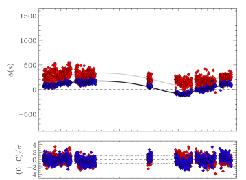
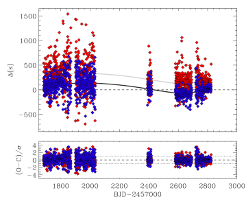
Figure 8: Same as Figure 2 but for TIC 219900027.

where $P_{2}$ and $T_{2}$ are the orbital period and the time of periastron passage of the third component’s relative orbit, respectively. In our ETV analysis, we also accounted for non-circular inner orbits, which result in a measurable displacement of the secondary ETV curve with respect to the primary one (see Figure 8 in Appendix B). Thus, for secondary eclipses, the term $-\,(T_{\rm s}-T_{\rm p})$ has to be added to the right side of Equation (11). It corresponds to the time interval between the primary and secondary eclipses (Kopal 1959; Hilditch 2001):

$$\frac{2\pi\,(T_{\rm s}-T_{\rm p})}{P_{1}+c_{1}}=\pi+2\tan^{-1}\frac{e_{1}\cos\omega_{1}}{(1-e_{1}^{2})^{1/2}}+\frac{2e_{1}\cos\omega_{1}\,(1-e_{1}^{2})^{1/2}}{(1-e_{1}^{2}\sin^{2}\omega_{1})},$$ (15)

where $e_{1}$ and $\omega_{1}$ are the eccentricity and the argument of periastron of the eclipsing pair, respectively. In summary, our ETV model consists of the parameters $\Theta=(c_{0},c_{1},e_{1},\omega_{1},e_{2},\omega_{2},P_{2},T_{2},A_{\rm LTTE})$.

In this work, we aim to demonstrate the feasibility of accurately measuring the third-body parameters from the ETV analysis of FFI targets. Therefore, we processed the two sets of ETV curves, derived from the corresponding FFI and SC light curves, independently. Another important aspect of our analysis is the determination of reliable uncertainties on the derived parameters. For this, we performed an initial fit of each ETV curve using a chain of $10^{6}$ points. Based on the best-fit preliminary solution, we applied an iterative 4$\sigma$-clipping technique to exclude possible outliers. In each iteration, we first computed the normalized chi-squared ($\chi^{2}/N$) of the best fit for both the primary and secondary ETV curves. Then, we rescaled the error bars of the primary and secondary eclipse times by multiplying them by $\sqrt{\chi^{2}_{\rm p}/N_{\rm p}}$ and $\sqrt{\chi^{2}_{\rm s}/N_{\rm s}}$, respectively. We removed the 4$\sigma$ outliers, and repeated the above steps until no more outliers were found. In order to obtain reliable uncertainties on the fitted parameters, we performed a new fit of the ETV curves using the rescaled error bars. Finally, we checked that the best-fit solution has $\chi^{2}_{\rm p}/N_{\rm p}\sim 1$ and $\chi^{2}_{\rm s}/N_{\rm s}\sim 1$ and that the mean error on primary and secondary eclipse times is of the same order of magnitude as the root mean square (rms) of the primary and secondary ETV residuals. The best-fit ETV solutions of our five targets are shown in Figure 2 and Appendix B. The values derived from the ETV fits of the SC data are given in Table 3 and Appendix C, together with their uncertainties.

Table 3: Best-fit orbital parameters for TIC 356896561 obtained from the SC data.

		84 per cent	16 per cent
Parameter	Median	interval	interval
$P_{\rm A}$ (d)	$2.253\,360405$	$+0.000\,000047$	$-0.000\,000046$
$T_{0}$ (BJD$-245\,7000$)	$1685.408\,645$	$+0.000\,013$	$-0.000\,010$
$e_{\rm A}$	0 (fixed)
$\omega_{\rm A}$ (∘)	0 (fixed)
$A_{\rm LTTE}$ (s)	51.2	+1.1	$-$1.1
$K_{\rm A}$ (km s-1)	2.34	+0.05	$-$0.05
$P_{\rm AB}$ (d)	477.5	+2.1	$-$2.0
$T_{\rm AB}$ (BJD$-245\,7000$)	2600.5	+8.2	$-$8.6
$e_{\rm AB}$	0.0054	+0.0074	$-$0.0040
$\omega_{\rm AB}$ (∘)	10.3	+6.2	$-$6.5
$a_{\rm A}\sin i_{\rm AB}$ (au)	0.1026	+0.0022	$-$0.0022
$f\!$($M_{\rm B}$) (M⊙)	0.000631	+0.000042	$-$0.000040
$M_{\rm B}\,(i_{\rm AB}\!=90^{\circ}$) (M⊙)	0.1425	+0.0033	$-$0.0033
$M_{\rm B}\,(i_{\rm AB}\!=90^{\circ}$) (MJup)	149.3	+3.4	$-$3.5
${\mathcal{A}}_{\rm dyn}/{\mathcal{A}}_{\rm LTTE}$	0.1901	+0.0014	$-$0.0014

4 Discussion

4.1 Comparison between SC and FFI results

In Section 3.3, we summarized the ETV analysis of five newly detected triple systems using the SC and FFI datasets independently. This allowed us to derive the orbital parameters of each system as listed in Table 3 and Appendix C. In principle, the mass of the third body can be obtained from Kepler’s third law applied to the EB’s barycentric orbit, namely:

$$\frac{M_{\rm B}^{3}}{(M_{\rm A}+M_{\rm B})^{2}}=\frac{a_{\rm A}^{3}}{P_{\rm AB}^{2}},$$ (16)

where $M_{\rm A}=M_{\rm Aa}+M_{\rm Ab}$ is the sum of the masses of the eclipsing components Aa and Ab. Here, the projected semi-major axis $a_{\rm A}\sin i_{\rm AB}$ is related to $A_{\rm LTTE}$ by Equation (12). We can then write the mass function of the third body as

$$f(M_{\rm B})=\frac{M_{\rm B}^{3}\,\sin^{3}i_{\rm AB}}{(M_{\rm Aa}+M_{\rm Ab}+M_{\rm B})^{2}}=1.074\times 10^{-3}\,\frac{A_{\rm LTTE}^{3}}{P_{\rm AB}^{2}},$$ (17)

where the masses are expressed in the units of solar mass, $A_{\rm LTTE}$ is in seconds, and $P_{\rm AB}$ is in days. Assuming an inclination of $i_{\rm AB}\!=90^{\circ}$, Equation (17) provides a lower limit on the mass $M_{\rm B}$ of the third component. Unfortunately, the masses of the eclipsing components, $M_{\rm Aa}$ and $M_{\rm Ab}$, are not presently known for the systems studied in this paper. Thus, for our calculations, we randomly drew $900\,000$ values of $M_{\rm Aa}$ and $M_{\rm Ab}$, corresponding to 90 per cent of the chain length after rejection of the burn-in phase, from a normal distribution centered on 1.00$\,{\rm M}_{\odot}$ with a standard deviation of $0.01\,{\rm M}_{\odot}$. We solved the mass function for the minimum tertiary mass by means of Laguerre’s method (Press et al., 1992), using the posterior distribution samples of $A_{\rm LTTE}$ and $P_{\rm AB}$ obtained from our MCMC fitting in Section 3.3. We then computed the median and the 16 per cent and 84 per cent credible intervals on the minimum tertiary mass from the corresponding posterior probability distribution. For each system, we listed in Table 4 the values of $a_{\rm A}\sin i_{\rm AB}$, $P_{\rm AB}$, and $M_{\rm B}$ derived from both the SC and FFI datasets, and we compared them in Figure 3.

Table 4: Derived values of $a_{\rm A}\sin i_{\rm AB}$, $P_{\rm AB}$, and $M_{\rm B}$ for the five systems.

TIC	$a_{\rm A}\sin i_{\rm AB}$	$P_{\rm AB}$	$M_{\rm B}\,(i_{\rm AB}\!=90^{\circ}$)	Obs. mode
	(au)	(d)	(M⊙)
219900027	$0.2466^{+0.0062}_{-0.0059}$	$1179.0^{+3.1}_{-8.1}$	$0.1904^{+0.0049}_{-0.0041}$	SC
	$0.206^{+0.019}_{-0.019}$	$1236.1^{+84.5}_{-39.1}$	$0.151^{+0.018}_{-0.017}$	FFI
229771234	$0.360^{+0.011}_{-0.010}$	$359.8^{+0.8}_{-0.8}$	$0.706^{+0.026}_{-0.025}$	SC
	$0.316^{+0.027}_{-0.026}$	$361.7^{+4.0}_{-3.9}$	$0.600^{+0.063}_{-0.056}$	FFI
259006185	$0.0773^{+0.0027}_{-0.0027}$	$199.6^{+0.5}_{-0.5}$	$0.1953^{+0.0072}_{-0.0072}$	SC
	$0.0716^{+0.0051}_{-0.0048}$	$199.8^{+0.9}_{-0.9}$	$0.180^{+0.014}_{-0.013}$	FFI
356896561	$0.1026^{+0.0022}_{-0.0022}$	$477.5^{+2.1}_{-2.0}$	$0.1425^{+0.0033}_{-0.0033}$	SC
	$0.1084^{+0.0037}_{-0.0037}$	$485.2^{+4.5}_{-3.9}$	$0.1493^{+0.0055}_{-0.0053}$	FFI
424461577	$0.6322^{+0.0038}_{-0.0037}$	$991.9^{+4.8}_{-4.0}$	$0.6167^{+0.0056}_{-0.0056}$	SC
	$0.605^{+0.021}_{-0.025}$	$990.7^{+42.6}_{-20.8}$	$0.583^{+0.031}_{-0.034}$	FFI

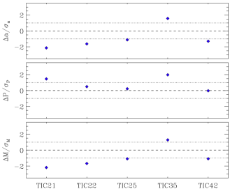
Figure 3: Difference in standard deviations between the system parameter estimates obtained from the two datasets. The top, middle, and bottom panels show the difference in $a_{\rm A}\sin i_{\rm AB}$, $P_{\rm AB}$, and $M_{\rm B}$, respectively.

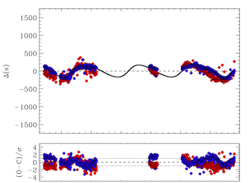
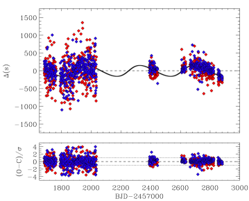
Figure 9: Same as Figure 2 but for TIC 229771234.

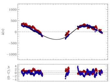
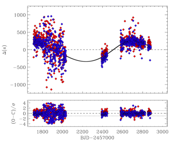
Figure 11: Same as Figure 2 but for TIC 424461577.

Based on our analysis of the SC and FFI data, we derived the minimum tertiary mass for each system with a precision better than 4 per cent and 12 per cent, respectively. Furthermore, as can be seen in Figure 3, the minimum mass value determined from the FFI data is underestimated (by more than 1$\sigma$) for four of the five systems considered. The minimum mass is related to the semi-major axis and thus to $A_{\rm LTTE}$ via Kepler’s third law, implying that the latter was underestimated during the fitting procedure (see top panel of Figure 3). Interestingly, we notice that the tighter the binary, the higher the mass discrepancy. According to the morphological classification described in Matijevič et al. (2012), our target sample can be divided into three categories: detached (TIC 259006185 and TIC 356896561), semi-detached (TIC 219900027 and TIC 424461577), and contact (TIC 229771234). For the two detached binaries, TIC 259006185 and TIC 356896561, we were able to reach a precision on the minimum tertiary mass better than 8 per cent using the FFI data, with a mass discrepancy lower than 1.3$\sigma$. The rms of the primary and secondary ETV residuals are of the order of 20 and 40 s, respectively. We obtained comparable results for the semi-detached binary TIC 424461577, despite the large scatter of the ETVs (rms of $\sim$200 s). The ETV amplitude observed for this system ($A_{\rm LTTE}\simeq$ 315 s) is indeed high enough to allow us to properly constrain the minimum tertiary mass. The two remaining binaries, TIC 219900027 and TIC 229771234, have the highest morphology values in our sample, i.e. 0.684 and 0.722, respectively. Their ETV curves are affected by a large scatter of 160–210 s for the primary and 270–300 s for the secondary. As a consequence, both the precision ($>$10 per cent) and accuracy ($>$1.5$\sigma$) of the minimum tertiary mass are degraded. For the three latter binaries, we found that the change of the FFI cadence from 30 to 10 minutes improves the quality of the timing significantly. This can be seen in Figures 8, 9, and 11 in Appendix B by comparing the scatter of the ETVs before and after BJD 245 9060, which corresponds to the last day of the 30-min cadence observations (Sector 27). It is thus expected that the new 200-s FFI cadence will significantly improve our ability to detect and characterize stellar and substellar companions around the shortest-period EBs. Although based on a small number of objects, these results highlight the importance of using the calibrated SC data to validate the ETV analysis of FFI targets.

4.2 Global properties of the systems

In this section, we discuss the global properties of each of the five investigated systems based on our results and the literature.

4.2.1 TIC 259006185

TIC 259006185 is a detached EB consisting of two unequal mass components in a $\sim$1.9-d circular orbit. Its light curve exhibits shallow secondary eclipses that were discarded from the final analysis due to their low signal-to-noise ratio. The LTTE solution suggests the presence of a minimum 0.20$\,{\rm M}_{\odot}$ companion orbiting the eclipsing pair with a short period of about 200 d. In such a compact orbital configuration, the EB system is expected to experience significant dynamical perturbations from the third body. Using Equations (10) and (12), we computed the ratio of the amplitudes of the dynamical and LTTE effects, ${\mathcal{A}}_{\rm dyn}/{\mathcal{A}}_{\rm LTTE}$, which is found to be 0.6. Such a result implies that the dynamical contribution is no longer negligible with respect to the LTTE contribution. While our LTTE model is sufficient to compare the ETV curves from the two datasets, a more detailed analysis is required to properly constrain the minimum mass of the third body. We also point out that the observed ETV curve of TIC 259006185 can be explained by the presence of migrating spots on the surface of either or both stars. Indeed, it was shown by Tran et al. (2013) that migrating spots can produce ETVs with typical periods of the order of 50–200 d and induce an anticorrelated behavior of the primary and secondary minima variations. Most of our systems exhibit such spot-induced ETVs, as can be seen in the residuals of Figures 2, 9, and 11. Unfortunately, in the absence of precise ETV measurements of the secondary eclipses, it is impossible to determine the origin of the primary ETV signal observed for TIC 259006185.

4.2.2 TIC 229771234 and TIC 424461577

As a result of our analysis, we identified two new compact hierarchical triples with outer periods less than 1000 d, namely TIC 229771234 ($P_{\rm AB}=359.8\,$d) and TIC 424461577 ($P_{\rm AB}=991.9\,$d). For both systems, the minimum mass of the third component (0.6–0.7$\,{\rm M}_{\odot}$) is consistent with that of a main-sequence K-type star. As noted by Tokovinin (2014), CHTs are rare among the entire population of hierarchical triples. They are thought to form differently than wider triple systems, most likely through a sequential disk fragmentation mechanism (Tokovinin & Moe, 2020; Tokovinin, 2021). From their ETV analysis of Kepler targets, Borkovits et al. (2016) provided the largest sample of short-outer-period triples to date, which contains 104 CHTs. In particular, they noted a deficit of short-period EBs ($P_{\rm A}\lesssim 1\,$d) with a close tertiary companion ($P_{\rm AB}\lesssim 200\,$d), suggesting additional differences between the formation of the tightest binaries and that of their longer-period counterparts. In order to better constrain the formation mechanisms of close binaries, it is thus important to increase the sample of well-characterized CHTs, especially those with binary periods $\lesssim\,$1 d such as TIC 229771234 ($P_{\rm A}=0.821\,$d) and TIC 424461577 ($P_{\rm A}=0.745\,$d). The example of TIC 229771234 demonstrates the potential of our method for recovering ETV signals with semi-amplitudes as low as 180 s (typical rms of 210 s) using the FFIs. For the shortest-period EBs, the ETV amplitude induced by a stellar companion in a 50-d orbit is expected to be $\sim$50 s (Borkovits et al., 2016), i.e., of the same order as the scatter of the primary ETV measurements obtained for TIC 229771234 and TIC 424461577 from the SC data (rms of 20–90 s). Thus, detecting the tightest CHTs (those with $P_{\rm A}\lesssim 1\,$d and $P_{\rm AB}\lesssim 200\,$d) represents a real challenge that requires a systematic follow-up, based on TESS SC photometry, of the most promising candidates.

For completeness, we also computed the expected radial velocity (RV) semi-amplitude induced by the companion on the EB, which is defined as

$$K_{\rm A}=\frac{21.80\,A_{\rm LTTE}}{P_{\rm AB}\,(1-e_{\rm AB}^{2})^{1/2}},$$ (18)

where $K_{\rm A}$ is in units of km s^-1, $A_{\rm LTTE}$ is in units of seconds, and $P_{\rm AB}$ is in units of days. We found the RV semi-amplitudes for TIC 229771234 and TIC 424461577 to be easily measurable with modern spectrographs, namely $K_{\rm A}=11.6$ and 7.1 km s^-1, respectively. By fitting a double-Keplerian orbit, it will then be possible to constrain the semi-amplitude of the ETV signal, the individual masses of the eclipsing components and, thus, the minimum mass of the circumbinary companion (see e.g. Marcadon et al. 2020).

4.2.3 TIC 219900027

TIC 219900027 (AU Dra) is known as a semi-detached EB with an orbital period of 0.515 d (Blattler, 1998; Sarounova et al., 1998). In contrast to the other systems studied here, the inner orbit of TIC 219900027 is found to be slightly eccentric ($e_{\rm A}=0.051^{+0.005}_{-0.013}$), as evidenced by the displacement of the secondary ETV curve with respect to the primary one (see Figure 8 in Appendix B). We identified the companion as being a low-mass red dwarf, with a minimum mass of about 0.19 M_⊙, orbiting the eclipsing pair in a $\sim$3.2-yr eccentric orbit ($e_{\rm AB}=0.424^{+0.012}_{-0.008}$). Additionally, a total of 69 times of minima were recorded in the $O-C$ gateway (Paschke & Brat, 2006) for the period 1956–2017, thereby allowing us to examine the long-term behavior of the measured ETVs. From the archival times of minima, we found that the orbital period of the eclipsing pair is continuously decreasing, which is suggested by a negative parabolic trend in the corresponding $O-C$ diagram. To account for the observed parabolic trend, a quadratic term, $c_{2}E^{2}$, has to be included in Equation (11). The rate of period change can then be estimated from the relation $\dot{P}=2c_{2}/P$, where $c_{2}$ is a fitted parameter. Orbital period changes are commonly observed in close EBs (Hong et al., 2022), and may result either from the effects of a magnetic activity cycle, known as the Applegate mechanism (Applegate, 1992), or from the mass transfer between the binary components. The long-term period decrease observed for TIC 219900027 may indicate that the EB is undergoing mass transfer accompanied by angular momentum loss, leading to a shrinkage of its orbit. A detailed period-change analysis of the system, which is beyond the scope of this paper, could shed some light on its past and future evolution.

4.2.4 TIC 356896561

Among the five studied systems, TIC 356896561 has the tertiary companion with the lowest minimum mass, namely $M_{\rm B}=0.143\,{\rm M}_{\odot}(=149\,{\rm M}_{\rm Jup})$. For our calculations, we assumed the individual masses of the eclipsing components to be $M_{\rm Aa}=M_{\rm Ab}=1.00\pm 0.01\,{\rm M}_{\odot}$. If we consider now a low-mass EB with component masses of $M_{\rm Aa}=M_{\rm Ab}=0.300\pm 0.003\,{\rm M}_{\odot}$, we find that the minimum tertiary mass is $M_{\rm B}=68.5\pm 1.6\,{\rm M}_{\rm Jup}$, which is below the hydrogen-burning mass limit of $\sim$80$\,{\rm M}_{\rm Jup}$ that separates brown dwarfs (BDs) from very low-mass stars (Baraffe et al., 2002). TIC 356896561 may therefore consist of a low-mass EB orbited by a possible BD-mass companion in a $\sim$1.3-yr orbit. This demonstrates the feasibility of detecting circumbinary companions with masses as low as those of BDs around low-mass EBs using the FFIs. Furthermore, the EB orbit is expected to undergo dynamical perturbations caused by the close-orbiting low-mass companion, as previously mentioned in Section 3.3. Borkovits et al. (2016) suggested a threshold value of ${\mathcal{A}}_{\rm dyn}/{\mathcal{A}}_{\rm LTTE}\sim 0.25$ above which a combined dynamical and LTTE model may be required. We derived the expected amplitude of the dynamical ETV contribution from Equation (10) by adopting $M_{\rm A}=0.6\,{\rm M}_{\odot}$ and $M_{\rm B}=0.065\,{\rm M}_{\odot}(=68.5\,{\rm M}_{\rm Jup})$. We obtained ${\mathcal{A}}_{\rm dyn}\simeq 14\,$s, leading to a ratio ${\mathcal{A}}_{\rm dyn}/{\mathcal{A}}_{\rm LTTE}\sim 0.27$, which is very close to the threshold value. In addition, the dynamical amplitude is found to be of the same order as the rms scatter in the ETV residuals ($\sim$10–20 s for the SC dataset), implying that the dynamical contribution to the ETVs cannot be properly assessed. Therefore, we limited our analysis to a simple LTTE model.

TIC 356896561 (GZ Dra, WDS 18127+5446) is classified as a visual binary in the Washington Double Star Catalog (WDS; Mason et al. 2001). This suggests that the EB+BD system may be gravitationally bound to a fourth body that corresponds to the secondary component of the visual pair. We attempted to determine the orbital period of the fourth body by using the position measurements found in the literature. We approximated the angular semi-major axis of the visual pair as the mean of the measured angular separations listed in Table 5. We then computed the absolute semi-major axis by adopting the trigonometric parallax of $4.84\pm 1.66\,$mas from Perryman et al. (1997), and found it to be $\sim$78 au. Finally, adopting this value and assuming a total mass of 3$\,{\rm M}_{\odot}$, we derived an orbital period of about 400 years for the visual pair from Kepler’s third law, making confirmation of its gravitationally-bound nature impossible. We also found eight additional eclipse times in the $O-C$ gateway and saw no evidence of a long-term trend caused by a fourth body.

Table 5: Relative positions of the two visual components of TIC 356896561.

Time	Angle	Separation	Reference
Bess. yr.	(∘)	(″)
1983.42	355.1	0.370	Muller (1984)
1983.52	348.6	0.380	Muller (1984)
1983.54	343.7	0.380	Muller (1984)
1985.50	348.7	0.330	Heintz (1987)
1991.25	343.0	0.428	Perryman et al. (1997)
1991.73	346.8	0.450	Fabricius et al. (2002)
1992.10	341.6	0.340	Muller (1997)
1995.64	347.9	0.350	Heintz (1996)

5 Summary and future prospects

In this study, we aimed to explore the feasibility of performing precise eclipse timing of TESS EBs using the FFIs. To this end, we developed a fast, automated method, based on a Bayesian approach, and applied it successfully to a sample of $\sim$100 EBs selected from the Villanova TESS EB catalog. After visual inspection of the $O-C$ diagrams, we identified a total of ten triple system candidates with outer periods less than $\sim$1300 d. For five of them, we were able to properly constrain the outer orbit from the SC and FFI data independently, thanks to the good coverage of the photometric observations in each mode, and to derive the minimum mass of the third component with a precision better than 4 per cent and 12 per cent, respectively. This approach allowed us to compare the results obtained from the two datasets. Thus, we found that using the FFI data results in the degradation of both the accuracy and precision of the tertiary mass determination for the tightest EBs and in the underestimation of the third component’s mass. However, we stress that the main results obtained from the FFI data regarding the nature of the detected signals are consistent with those obtained from the SC data. Our main findings and prospects are as follows.

1. CHTs are rare, and their detection is challenging as the amplitude of the ETV signal decreases with decreasing outer period. This was pointed out by Borkovits et al. (2016), who noticed the almost complete absence of short-period EBs with a close tertiary companion (i.e. with $P_{\rm AB}\lesssim 200\,$d) among their sample of 222 Kepler triple candidates. Furthermore, due to their compactness, CHTs are of particular interest for our understanding of the formation (Tokovinin, 2021) and evolution (Toonen et al., 2020, 2022) of hierarchical triple stellar systems. In this study, we report the detection of two new CHTs, TIC 229771234 and TIC 424461577, with respective outer periods of 359.8 and 991.9 d. For TIC 229771234, we were able to recover the low-amplitude signal of the close companion from the FFIs, despite the large scatter of the ETV measurements. Based on these results, we may expect to find more of these systems by conducting a systematic search for ETVs among TESS FFI EBs. Additionally, we argue that detecting the tightest CHTs will require a dedicated photometric survey based on TESS SC data. In this context, the Gaia Data Release 3 (DR3) non-single-stars (NSS) catalog (Gaia Collaboration, 2022) represents a powerful tool for identifying the most promising CHT candidates, as recently shown by Czavalinga et al. (2023).

2. The BD desert refers to the low occurence of BD companions around main-sequence stars with periods shorter than $\sim$5 yr (Grether & Lineweaver, 2006). This desert is particularly pronounced in the mass range 35$-$55$\,{\rm M}_{\rm Jup}$ and might indicate different formation mechanisms for close-orbiting BDs and isolated ones (Ma & Ge, 2014). BDs are generally believed to form like stars, through the fragmentation of molecular clouds (Padoan & Nordlund, 2004). However, Ma & Ge (2014) suggested the existence of two populations of BD companions, distinguishable by their physical and orbital properties, as recently confirmed by Stevenson et al. (2023) from a larger sample of BDs. One of them consists of high-mass BDs formed via molecular cloud fragmentation, while the other consists of low-mass BDs that are thought to be formed by disk instability in the same manner as planets (Boss, 1997). In this work, we identified a possible BD companion orbiting the eclipsing binary TIC 356896561 with a relatively short period of $\sim$1.3 yr, placing it in the BD desert. Based on their spectroscopic survey of 47 single-lined EBs, Martin et al. (2019) reported the absence of circumbinary BDs with orbital periods less than 6000 d, suggesting the existence of a BD desert around binary stars that needs to be confirmed. Using numerical simulations, Getley et al. (2021) investigated the potential of the ETV method in detecting BD-mass companions in close orbits and concluded that the BD desert is not due to detection limits. Therefore, to improve our understanding of the BD desert, we aim to increase the number of confirmed circumbinary BDs by taking advantage of the large sample of EBs expected to be detected in the TESS FFIs.

3. In addition to the LTTE, there are several other effects that can produce ETVs, such as starspot migration, apsidal motion, and mass transfer. Spot-induced ETVs have typical periods of $\sim$50–200 d and show a distinctive anticorrelated pattern between the primary and secondary minima variations, as indicated by Tran et al. (2013). Three of our five EBs exhibit such spot-induced variations, and we suspect that the $\sim$200-d signal found in the $O-C$ diagram of TIC 259006185 may be caused by the presence of migrating starspots rather than by a third body. Balaji et al. (2015) presented a detailed analysis of 414 Kepler binaries with anticorrelated primary and secondary ETVs. They investigated the effect of differential stellar rotation on the relative motions of spots and found that the differential rotation of stars in tight binaries is less pronounced than that of single stars. The reason for this difference remains to be understood. In contrast to the spot-induced variations, ETVs caused by apsidal motion or mass transfer occur on long time-scales and require decades of observations from ground- and space-based telescopes to be detected. The analysis of these long-term variations has important implications for a variety of studies. For example, by measuring the apsidal motion in eccentric EBs, it is possible to test general relativity (Baroch et al., 2021) and stellar structure models (Claret et al., 2021). In the framework of the Contact Binaries Towards Merging (CoBiToM) Project, Gazeas et al. (2021) and Loukaidou et al. (2022) investigated the evolution of ultra-short-period contact binaries through the analysis of their $O-C$ curves, which were obtained during a decades-long monitoring program. These examples highlight the importance of extending the time span of the observations using the high-precision photometric data provided by the TESS mission.
   

This paper includes data collected by the TESS mission, which are publicly available from the MAST. Funding for the TESS mission is provided by NASA’s Science Mission directorate. This research has made use of NASA’s Astrophysics Data System Bibliographic Services, the SIMBAD data base, operated at CDS, Strasbourg, France and the VizieR catalogue access tool, CDS, Strasbourg, France. The original description of the VizieR service was published in Ochsenbein et al. (2000).

We gratefully acknowledge support from the NASA TESS Guest Investigator grant 80NSSC22K0180 (PI: A. Prša).

Appendix A Light curves

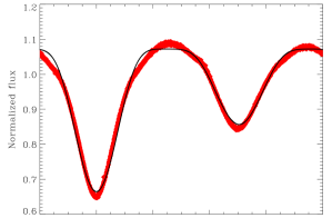
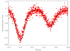
Figure 4: Same as Figure 1 but for TIC 219900027 (presented here is Sector 19).

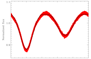
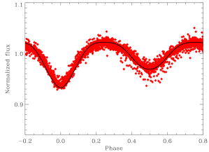
Figure 5: Same as Figure 1 but for TIC 229771234 (presented here is Sector 52). To account for the eclipse depth difference between the SC and FFI light curves, we derived an independent light-curve solution for each of the two datasets.

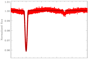
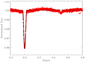
Figure 6: Same as Figure 1 but for TIC 259006185 (presented here is Sector 55).

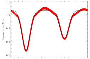
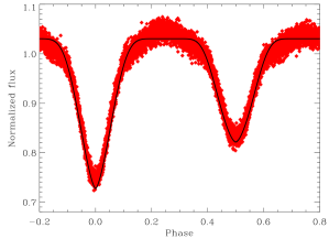
Figure 7: Same as Figure 1 but for TIC 424461577 (presented here is Sector 57).

Appendix B Eclipse timing variation diagrams

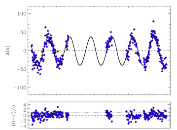
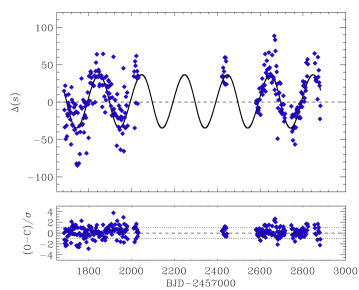
Figure 10: Same as Figure 2 but for TIC 259006185.

Appendix C Tables of orbital parameters

Table 6: Best-fit orbital parameters for TIC 219900027 obtained from the SC data.

		84 per cent	16 per cent
Parameter	Median	interval	interval
$P_{\rm A}$ (d)	$0.515\,262789$	$+0.000\,000014$	$-0.000\,000021$
$T_{0}$ (BJD$-245\,7000$)	$1683.749\,2859$	$+0.000\,0029$	$-0.000\,0041$
$e_{\rm A}$	0.051	$+0.005$	$-$0.013
$\omega_{\rm A}$ (∘)	263.4	$+0.6$	$-$2.1
$A_{\rm LTTE}$ (s)	123.1	+3.1	$-$2.9
$K_{\rm A}$ (km s-1)	2.51	+0.07	$-$0.05
$P_{\rm AB}$ (d)	1179.0	+3.1	$-$8.1
$T_{\rm AB}$ (BJD$-245\,7000$)	2573.7	+33.8	$-$7.8
$e_{\rm AB}$	0.424	+0.012	$-$0.008
$\omega_{\rm AB}$ (∘)	253.3	+10.3	$-$4.8
$a_{\rm A}\sin i_{\rm AB}$ (au)	0.2466	+0.0062	$-$0.0059
$f\!$($M_{\rm B}$) (M⊙)	0.00144	+0.00011	$-$0.00008
$M_{\rm B}\,(i_{\rm AB}\!=90^{\circ}$) (M⊙)	0.1904	+0.0049	$-$0.0041
${\mathcal{A}}_{\rm dyn}/{\mathcal{A}}_{\rm LTTE}$	0.002 973	+0.000 058	$-$0.000 047

Table 7: Best-fit orbital parameters for TIC 229771234 obtained from the SC data.

		84 per cent	16 per cent
Parameter	Median	interval	interval
$P_{\rm A}$ (d)	$0.820\,953946$	$+0.000\,000043$	$-0.000\,000049$
$T_{0}$ (BJD$-245\,7000$)	$1931.067\,665$	$+0.000\,016$	$-0.000\,041$
$e_{\rm A}$	0 (fixed)
$\omega_{\rm A}$ (∘)	0 (fixed)
$A_{\rm LTTE}$ (s)	179.7	+5.3	$-$5.2
$K_{\rm A}$ (km s-1)	11.6	+0.6	$-$0.5
$P_{\rm AB}$ (d)	359.8	+0.8	$-$0.8
$T_{\rm AB}$ (BJD$-245\,7000$)	2609.9	+1.4	$-$1.3
$e_{\rm AB}$	0.341	+0.067	$-$0.050
$\omega_{\rm AB}$ (∘)	0.25	+0.39	$-$0.18
$a_{\rm A}\sin i_{\rm AB}$ (au)	0.360	+0.011	$-$0.010
$f\!$($M_{\rm B}$) (M⊙)	0.0481	+0.0044	$-$0.0041
$M_{\rm B}\,(i_{\rm AB}\!=90^{\circ}$) (M⊙)	0.706	+0.026	$-$0.025
${\mathcal{A}}_{\rm dyn}/{\mathcal{A}}_{\rm LTTE}$	0.0480	+0.0056	$-$0.0033

Table 8: Best-fit orbital parameters for TIC 259006185 obtained from the SC data.

		84 per cent	16 per cent
Parameter	Median	interval	interval
$P_{\rm A}$ (d)	$1.939\,651524$	$+0.000\,000046$	$-0.000\,000044$
$T_{0}$ (BJD$-245\,7000$)	$1901.860\,271$	$+0.000\,031$	$-0.000\,052$
$e_{\rm A}$	0 (fixed)
$\omega_{\rm A}$ (∘)	0 (fixed)
$A_{\rm LTTE}$ (s)	38.6	+1.3	$-$1.3
$K_{\rm A}$ (km s-1)	4.2	+0.1	$-$0.1
$P_{\rm AB}$ (d)	199.6	+0.5	$-$0.5
$T_{\rm AB}$ (BJD$-245\,7000$)	2675.7	+20.0	$-$8.4
$e_{\rm AB}$	0.079	+0.062	$-$0.049
$\omega_{\rm AB}$ (∘)	147.9	+35.4	$-$14.9
$a_{\rm A}\sin i_{\rm AB}$ (au)	0.0773	+0.0027	$-$0.0027
$f\!$($M_{\rm B}$) (M⊙)	0.00154	+0.00016	$-$0.00015
$M_{\rm B}\,(i_{\rm AB}\!=90^{\circ}$) (M⊙)	0.1953	+0.0072	$-$0.0072
${\mathcal{A}}_{\rm dyn}/{\mathcal{A}}_{\rm LTTE}$	0.605	+0.014	$-$0.006

Table 9: Best-fit orbital parameters for TIC 424461577 obtained from the SC data.

		84 per cent	16 per cent
Parameter	Median	interval	interval
$P_{\rm A}$ (d)	$0.744\,836447$	$+0.000\,000046$	$-0.000\,000052$
$T_{0}$ (BJD$-245\,7000$)	$1712.098\,380$	$+0.000\,008$	$-0.000\,013$
$e_{\rm A}$	0 (fixed)
$\omega_{\rm A}$ (∘)	0 (fixed)
$A_{\rm LTTE}$ (s)	315.5	+1.9	$-$1.8
$K_{\rm A}$ (km s-1)	7.08	+0.05	$-$0.05
$P_{\rm AB}$ (d)	991.9	+4.8	$-$4.0
$T_{\rm AB}$ (BJD$-245\,7000$)	2560.1	+4.7	$-$4.8
$e_{\rm AB}$	0.204	+0.012	$-$0.008
$\omega_{\rm AB}$ (∘)	30.7	+1.7	$-$1.6
$a_{\rm A}\sin i_{\rm AB}$ (au)	0.6322	+0.0038	$-$0.0037
$f\!$($M_{\rm B}$) (M⊙)	0.03425	+0.00070	$-$0.00067
$M_{\rm B}\,(i_{\rm AB}\!=90^{\circ}$) (M⊙)	0.6167	+0.0056	$-$0.0056
${\mathcal{A}}_{\rm dyn}/{\mathcal{A}}_{\rm LTTE}$	0.006 222	+0.000 033	$-$0.000 033

References

- Applegate (1992) Applegate, J. H. 1992, ApJ, 385, 621, doi: 10.1086/170967
- Balaji et al. (2015) Balaji, B., Croll, B., Levine, A. M., & Rappaport, S. 2015, MNRAS, 448, 429, doi: 10.1093/mnras/stv031
- Baraffe et al. (2002) Baraffe, I., Chabrier, G., Allard, F., & Hauschildt, P. H. 2002, A&A, 382, 563, doi: 10.1051/0004-6361:20011638
- Baroch et al. (2021) Baroch, D., Giménez, A., Ribas, I., et al. 2021, A&A, 649, A64, doi: 10.1051/0004-6361/202040004
- Benbakoura et al. (2021) Benbakoura, M., Gaulme, P., McKeever, J., et al. 2021, A&A, 648, A113, doi: 10.1051/0004-6361/202037783
- Blattler (1998) Blattler, E. 1998, Information Bulletin on Variable Stars, 4587, 1
- Borkovits (2022) Borkovits, T. 2022, Galaxies, 10, 9, doi: 10.3390/galaxies10010009
- Borkovits et al. (2016) Borkovits, T., Hajdu, T., Sztakovics, J., et al. 2016, MNRAS, 455, 4136, doi: 10.1093/mnras/stv2530
- Borkovits et al. (2015) Borkovits, T., Rappaport, S., Hajdu, T., & Sztakovics, J. 2015, MNRAS, 448, 946, doi: 10.1093/mnras/stv015
- Boss (1997) Boss, A. P. 1997, Science, 276, 1836, doi: 10.1126/science.276.5320.1836
- Brasseur et al. (2019) Brasseur, C. E., Phillip, C., Fleming, S. W., Mullally, S. E., & White, R. L. 2019, Astrocut: Tools for creating cutouts of TESS images, Astrophysics Source Code Library, record ascl:1905.007. http://ascl.net/1905.007
- Claret et al. (2021) Claret, A., Giménez, A., Baroch, D., et al. 2021, A&A, 654, A17, doi: 10.1051/0004-6361/202141484
- Conroy et al. (2014) Conroy, K. E., Prša, A., Stassun, K. G., et al. 2014, AJ, 147, 45, doi: 10.1088/0004-6256/147/2/45
- Czavalinga et al. (2023) Czavalinga, D. R., Mitnyan, T., Rappaport, S. A., et al. 2023, A&A, 670, A75, doi: 10.1051/0004-6361/202245300
- Fabricius et al. (2002) Fabricius, C., Høg, E., Makarov, V. V., et al. 2002, A&A, 384, 180, doi: 10.1051/0004-6361:20011822
- Feinstein et al. (2019) Feinstein, A. D., Montet, B. T., Foreman-Mackey, D., et al. 2019, PASP, 131, 094502, doi: 10.1088/1538-3873/ab291c
- Gaia Collaboration (2022) Gaia Collaboration. 2022, VizieR Online Data Catalog, I/357
- Gazeas et al. (2021) Gazeas, K. D., Loukaidou, G. A., Niarchos, P. G., et al. 2021, MNRAS, 502, 2879, doi: 10.1093/mnras/stab234
- Getley et al. (2021) Getley, A. K., Carter, B., King, R., & O’Toole, S. 2021, MNRAS, 504, 4291, doi: 10.1093/mnras/stab1207
- Ginsburg et al. (2019) Ginsburg, A., Sipőcz, B. M., Brasseur, C. E., et al. 2019, AJ, 157, 98, doi: 10.3847/1538-3881/aafc33
- Grether & Lineweaver (2006) Grether, D., & Lineweaver, C. H. 2006, ApJ, 640, 1051, doi: 10.1086/500161
- Guerrero et al. (2021) Guerrero, N. M., Seager, S., Huang, C. X., et al. 2021, ApJS, 254, 39, doi: 10.3847/1538-4365/abefe1
- Hastings (1970) Hastings, W. K. 1970, Biometrika, 57, 97, doi: 10.1093/biomet/57.1.97
- Hatt et al. (2023) Hatt, E., Nielsen, M. B., Chaplin, W. J., et al. 2023, A&A, 669, A67, doi: 10.1051/0004-6361/202244579
- Heintz (1987) Heintz, W. D. 1987, ApJS, 65, 161, doi: 10.1086/191221
- Heintz (1996) —. 1996, ApJS, 105, 475, doi: 10.1086/192324
- Hełminiak et al. (2021) Hełminiak, K. G., Moharana, A., Pawar, T., et al. 2021, MNRAS, 508, 5687, doi: 10.1093/mnras/stab2963
- Hilditch (2001) Hilditch, R. W. 2001, An Introduction to Close Binary Stars
- Hong et al. (2022) Hong, K., Woo Lee, J., Park, J.-H., et al. 2022, AJ, 163, 157, doi: 10.3847/1538-3881/ac4e98
- Irwin (1952) Irwin, J. B. 1952, ApJ, 116, 211, doi: 10.1086/145604
- Jenkins et al. (2016) Jenkins, J. M., Twicken, J. D., McCauliff, S., et al. 2016, in Society of Photo-Optical Instrumentation Engineers (SPIE) Conference Series, Vol. 9913, Software and Cyberinfrastructure for Astronomy IV, ed. G. Chiozzi & J. C. Guzman, 99133E, doi: 10.1117/12.2233418
- Kopal (1959) Kopal, Z. 1959, Close binary systems
- Kruse et al. (2021) Kruse, E., Powell, B., Kostov, V., Schnittman, J., & Quintana, E. 2021, in Posters from the TESS Science Conference II (TSC2), 163, doi: 10.5281/zenodo.5131355
- Li et al. (2018) Li, T., Bedding, T. R., Huber, D., et al. 2018, MNRAS, 475, 981, doi: 10.1093/mnras/stx3079
- Loukaidou et al. (2022) Loukaidou, G. A., Gazeas, K. D., Palafouta, S., et al. 2022, MNRAS, 514, 5528, doi: 10.1093/mnras/stab3424
- Ma & Ge (2014) Ma, B., & Ge, J. 2014, MNRAS, 439, 2781, doi: 10.1093/mnras/stu134
- Marcadon et al. (2020) Marcadon, F., Hełminiak, K. G., Marques, J. P., et al. 2020, MNRAS, 499, 3019, doi: 10.1093/mnras/staa3040
- Martin et al. (2019) Martin, D. V., Triaud, A. H. M. J., Udry, S., et al. 2019, A&A, 624, A68, doi: 10.1051/0004-6361/201833669
- Marzari & Thebault (2019) Marzari, F., & Thebault, P. 2019, Galaxies, 7, 84, doi: 10.3390/galaxies7040084
- Mason et al. (2001) Mason, B. D., Wycoff, G. L., Hartkopf, W. I., Douglass, G. G., & Worley, C. E. 2001, AJ, 122, 3466, doi: 10.1086/323920
- Matijevič et al. (2012) Matijevič, G., Prša, A., Orosz, J. A., et al. 2012, AJ, 143, 123, doi: 10.1088/0004-6256/143/5/123
- Mayer (1990) Mayer, P. 1990, Bulletin of the Astronomical Institutes of Czechoslovakia, 41, 231
- Metropolis et al. (1953) Metropolis, N., Rosenbluth, A. W., Rosenbluth, M. N., Teller, A. H., & Teller, E. 1953, J. Chem. Phys., 21, 1087, doi: 10.1063/1.1699114
- Mikulášek (2015) Mikulášek, Z. 2015, A&A, 584, A8, doi: 10.1051/0004-6361/201425244
- Moharana et al. (2023) Moharana, A., Hełminiak, K. G., Marcadon, F., et al. 2023, MNRAS, 521, 1908, doi: 10.1093/mnras/stad622
- Moharana et al. (2024) —. 2024, MNRAS, 527, 53, doi: 10.1093/mnras/stad3117
- Muller (1984) Muller, P. 1984, A&AS, 57, 467
- Muller (1997) —. 1997, A&AS, 126, 273, doi: 10.1051/aas:1997387
- Nardiello (2020) Nardiello, D. 2020, MNRAS, 498, 5972, doi: 10.1093/mnras/staa2745
- Ochsenbein et al. (2000) Ochsenbein, F., Bauer, P., & Marcout, J. 2000, A&AS, 143, 23, doi: 10.1051/aas:2000169
- Padoan & Nordlund (2004) Padoan, P., & Nordlund, Å. 2004, ApJ, 617, 559, doi: 10.1086/345413
- Paschke & Brat (2006) Paschke, A., & Brat, L. 2006, Open European Journal on Variable Stars, 23, 13
- Perryman et al. (1997) Perryman, M. A. C., Lindegren, L., Kovalevsky, J., et al. 1997, A&A, 323, L49
- Pietrzyński et al. (2019) Pietrzyński, G., Graczyk, D., Gallenne, A., et al. 2019, Nature, 567, 200, doi: 10.1038/s41586-019-0999-4
- Press et al. (1992) Press, W. H., Teukolsky, S. A., Vetterling, W. T., & Flannery, B. P. 1992, Numerical recipes in C. The art of scientific computing
- Prša et al. (2022) Prša, A., Kochoska, A., Conroy, K. E., et al. 2022, ApJS, 258, 16, doi: 10.3847/1538-4365/ac324a
- Raghavan et al. (2010) Raghavan, D., McAlister, H. A., Henry, T. J., et al. 2010, ApJS, 190, 1, doi: 10.1088/0067-0049/190/1/1
- Ricker et al. (2015) Ricker, G. R., Winn, J. N., Vanderspek, R., et al. 2015, Journal of Astronomical Telescopes, Instruments, and Systems, 1, 014003, doi: 10.1117/1.JATIS.1.1.014003
- Rowden et al. (2020) Rowden, P., Borkovits, T., Jenkins, J. M., et al. 2020, AJ, 160, 76, doi: 10.3847/1538-3881/ab9d20
- Sarounova et al. (1998) Sarounova, L., Wolf, M., & Borovicka, J. 1998, Information Bulletin on Variable Stars, 4605, 1
- Silva Aguirre et al. (2020) Silva Aguirre, V., Stello, D., Stokholm, A., et al. 2020, ApJ, 889, L34, doi: 10.3847/2041-8213/ab6443
- Smith et al. (2012) Smith, J. C., Stumpe, M. C., Van Cleve, J. E., et al. 2012, PASP, 124, 1000, doi: 10.1086/667697
- Stevenson et al. (2023) Stevenson, A. T., Haswell, C. A., Barnes, J. R., & Barstow, J. K. 2023, MNRAS, 526, 5155, doi: 10.1093/mnras/stad3041
- Stumpe et al. (2014) Stumpe, M. C., Smith, J. C., Catanzarite, J. H., et al. 2014, PASP, 126, 100, doi: 10.1086/674989
- Stumpe et al. (2012) Stumpe, M. C., Smith, J. C., Van Cleve, J. E., et al. 2012, PASP, 124, 985, doi: 10.1086/667698
- Tokovinin (2014) Tokovinin, A. 2014, AJ, 147, 87, doi: 10.1088/0004-6256/147/4/87
- Tokovinin (2021) —. 2021, Universe, 7, 352, doi: 10.3390/universe7090352
- Tokovinin & Moe (2020) Tokovinin, A., & Moe, M. 2020, MNRAS, 491, 5158, doi: 10.1093/mnras/stz3299
- Toonen et al. (2022) Toonen, S., Boekholt, T. C. N., & Portegies Zwart, S. 2022, A&A, 661, A61, doi: 10.1051/0004-6361/202141991
- Toonen et al. (2020) Toonen, S., Portegies Zwart, S., Hamers, A. S., & Bandopadhyay, D. 2020, A&A, 640, A16, doi: 10.1051/0004-6361/201936835
- Tran et al. (2013) Tran, K., Levine, A., Rappaport, S., et al. 2013, ApJ, 774, 81, doi: 10.1088/0004-637X/774/1/81
- Wolf et al. (2021) Wolf, M., Kučáková, H., Zasche, P., et al. 2021, A&A, 647, A65, doi: 10.1051/0004-6361/202039851
- Wolf et al. (2016) Wolf, M., Zasche, P., Kučáková, H., et al. 2016, A&A, 587, A82, doi: 10.1051/0004-6361/201527941
- Wolf et al. (2018) Wolf, M., Kučáková, H., Zasche, P., et al. 2018, A&A, 620, A72, doi: 10.1051/0004-6361/201833708