Genuine Knowledge from Practice:
Diffusion Test-Time Adaptation for Video Adverse Weather Removal

Abstract

Real-world vision tasks frequently suffer from the appearance of unexpected adverse weather conditions, including rain, haze, snow, and raindrops. In the last decade, convolutional neural networks and vision transformers have yielded outstanding results in single-weather video removal. However, due to the absence of appropriate adaptation, most of them fail to generalize to other weather conditions. Although ViWS-Net is proposed to remove adverse weather conditions in videos with a single set of pre-trained weights, it is seriously blinded by seen weather at train-time and degenerates when coming to unseen weather during test-time. In this work, we introduce test-time adaptation into adverse weather removal in videos, and propose the first framework that integrates test-time adaptation into the iterative diffusion reverse process. Specifically, we devise a diffusion-based network with a novel temporal noise model to efficiently explore frame-correlated information in degraded video clips at training stage. During inference stage, we introduce a proxy task named Diffusion Tubelet Self-Calibration to learn the primer distribution of test video stream and optimize the model by approximating the temporal noise model for online adaptation. Experimental results, on benchmark datasets, demonstrate that our Test-Time Adaptation method with Diffusion-based network(Diff-TTA) outperforms state-of-the-art methods in terms of restoring videos degraded by seen weather conditions. Its generalizable capability is also validated with unseen weather conditions in both synthesized and real-world videos.

1 Introduction

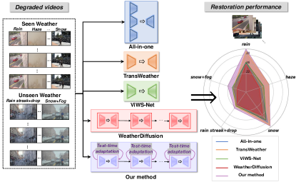
Figure 1: Overview of the existing all-in-one adverse weather removal methods. Our approach can achieve superior performance not only in seen weather conditions but also in unseen weather conditions with a single set of pre-trained weights by diffusion test-time adaptation. In particular, our Diff-TTA is 90$\times$ more efficient than WeatherDiffusion.

Adverse weather like rain, snow, and haze is very common in many existing outdoor videos. The presence of adverse weather usually decreases the visibility of the captured videos and significantly impairs the performance of subsequent high-level vision applications such as object detection, semantic segmentation and autonomous driving. To mitigate these negative effects, Convolutional Neural Networks (CNNs) and Transformers are frequently utilized in the literature. Also, Diffusion models have emerged as the de-facto generative model for image synthesis [16, 14, 37] and have been developed for single-image adverse weather removal [34]. While deep neural networks can achieve decent results on test points within the distribution, real-world applications often demand robustness. This is especially crucial when facing unknown input perturbations, changes in weather conditions, or other sources of distribution shift. Existing single-weather removal approaches [20, 61, 4] require follow-up training to adapt to specific domains. This leads to the switching between different parameter sets, which can make the pipeline cumbersome.

Figure 2: Our Diff-TTA enables weather removal models to overcome unseen weather corruptions. We use t-SNE [40] to visualize features from the last feature extractor layer of each dataset. Obviously, unseen data points tend to approximate the seen ones after adaptation, which means Diff-TTA can categorize unknown degradation into known distribution. (‘Real-world’ contains video clips simultaneously degraded by fog and snow.)

Recently, all-in-one adverse weather removal has attracted the attention of the community, which aims to handle diverse weather conditions with a generic model [21, 39, 11, 52]. However, the potential issue of frequently failing to recover from out-of-distribution conditions remains largely unaddressed due to the finiteness of training data and the absence of a test data adaptation mechanism. As shown in Figure 1, generic models suffer significant degradation when handling all the possible weather conditions beyond the scope of their training data. Furthermore, a common aspect among many real-world applications is the necessity for online adaptation with limited data. This is particularly relevant in scenarios such as autonomous vehicles or drones, where a vision model must continually process a video stream and adjust its predictions. To achieve effective adaptation, it is crucial to leverage the incoming data in a way that is beneficial and does not introduce harmful biases, even when there are distribution shifts between the training and test data. Thus, akin to how humans update knowledge through practice, the task of removing any weather condition through online adaptation using a single set of pre-trained weights is both pragmatic and promising, albeit challenging.

In this paper, we construct the diffusion-based framework for video adverse weather removal. Yet, diffusion models usually entail significant training overhead, hindering the technique’s broader adoption in the research community of video tasks. Instead of introducing massive parameters for temporal encoding, we design an efficient strategy based on DDIM [38] to preserve temporal correlation, specifically temporal noise model, in order to alleviate its training load. In contrast to the vanilla noise model, which independently samples noise for each frame from a standard Gaussian distribution, our temporal noise model takes into account the inter-frame relationship via time series models. More importantly, to promptly address unexpected weather conditions, we introduce test-time adaptation techniques by recalibrating the model’s parameters using only the degraded test data. The mainstream of test-time adaptation methods [41, 18, 60] manipulate and iteratively update the normalization statistics of CNNs and Vision Transformer using specific proxy tasks at the test phase. However, these methods often fail when transferring to low-level tasks. Additionally, incorporating such iterative adaptation into these models significantly increases the cost of inference, multiplying it by the number of iterations, compared to the original counterpart.

In contrast, we highlight the advantage of integrating the diffusion reverse process and test-time adaptation based on their common characteristics of iteration. As far as we know, there has been no work to emerge the possibility of Diffusion models and test-time adaptation. Based on our diffusion-based framework, we design a proxy task and efficiently incorporate it into each denoising iteration when reversing our temporal diffusion process. Specifically, we develop a surrogate task called Diffusion Tubelet Self-Calibration (Diff-TSC), which is supervised by temporal noise model. This is designed to be task-agnostic and does not require any alterations to the training procedure. Rather than directly traversing all fine-grained details, we extract a few tubelets to taste the primer distribution of the frames degraded by unknown weather. This approach facilitates rapid optimization of the diffusion model while also reducing computational costs. As displayed in Figure 2, test-time adaptation helps to improve the model’s robustness in real-world scenarios by mitigating the gap between seen and unseen weather corruptions.

Our contributions can be summarized as:

• We introduce the first diffusion-based framework for all-in-one adverse weather removal in videos. This framework efficiently leverages temporal redundancy information through the novel temporal noise model.

• To improve the model’s robustness against unknown weather, we are the first to introduce test-time adaptation by incorporating a proxy task into the diffusion reverse process to learn the primer distribution of the test data.

• We extensively evaluate our approach on seen weather (e.g., rain, haze, snow) and unseen weather (e.g., rain streak+raindrop, snow+fog). The superior performance over synthesized and real-world videos consistently validates its effectiveness and generalizable ability.

2 Related Work

All-in-one Adverse Weather Removal. Over the past decade, The community of low-level vision has paid much attention to single weather removal, e.g., deraining [5, 20, 24, 43, 48, 50, 51, 55], dehazing [36, 61, 28, 47], desnowing [9, 58, 4, 8, 7], both on the image level and the video level. Due to the limitations of existing models in adapting to different weather conditions, researchers have recently been investigating the use of a single model instance for multiple adverse weather removal tasks. At the image level, following the pioneering work All-in-one [21], TransWeather [39] and TKL [11] were introduced to tackle many weather conditions with the single encoder and decoder. Zhu et al. [64] elaborated a two-stage training strategy to explore the weather-general and weather-specific information for the sophisticated removal of diverse weather conditions. Ye et al. [54] introduced high-quality codebook priors learned by a pre-trained VQGAN to restore texture details from adverse weather degradation. The aforementioned methods failed to capture redundant information from temporal space. While they can be adapted for frame-by-frame adverse weather removal, incorporating temporal data in video-level methods provides a more robust solution for dealing with multiple adverse weather conditions in videos. Very recently, Yang [52] introduced ‘ViWS-Net’, the first video-level approach. This method uses weather messenger tokens to transfer weather knowledge across frames. It also employs adversarial learning to distinguish the weather type, thereby emphasizing weather-invariant information. However, they did not consider online adaptation of the deep model, making the potential collapse for unseen scenarios degraded by unknown weather.

Diffusion Models. Diffusion model is well-known as a generative modeling approach for its superior achievements in image synthesis and generation tasks [16, 14, 37, 53, 59, 27]. In essence, Denoising Diffusion Probabilistic Models (DDPM) [16] adopted parameterized Markov chain to optimize the lower variational bound on the likelihood function, which can simulate a diffusion process to iteratively improve the quality of target distribution than other generative models. For restoration tasks, Luo et al. [30] applied stochastic differential equations featuring mean reversion in diffusion models to improve low-quality images. DiffIR [46] provided a strong diffusion baseline for image restoration by estimating a compact IR prior representation. Zhang et al. [62] proposed a unified conditional framework based on diffusion models for image restoration by multi-source guidance of a lightweight U-Net. Özdenizci et al. [34] designed a patch-based diffusion modeling approach called WeatherDiffusion to make the network size-agnostic. While this technique utilizes diffusion models for image weather removal, its very slow inference speed restricts practical use. Nevertheless, there is no work adapting diffusion models to video adverse weather removal.

Test-time Adaptation. Recently, there has been a growing interest in adapting deep models using exclusively sequential, unlabeled test data. This contrasts with the traditional unsupervised domain adaptation, which asks the access to both training data and a sufficient amount of unlabeled test data. Test-time adaptation techniques allow for model updates using distributional statistics from either a single instance or batch of unlabeled test data. Typically, TENT [41] focuses on minimizing the model’s prediction entropy on the target data. T3A [18] adjusts the classifier of a trained source model by computing a pseudo-prototype representation of different classes using unlabeled test data. MEMO [60] aims to minimize marginal entropy, compelling the deep model to consistently predict across various augmentations. This approach enforces the invariances of these augmentations and ensures prediction confidence. Chen et al. [3] proposed to apply self-supervised contrastive learning for target feature learning, which was trained jointly with pseudo labeling. Although test-time adaptation methods are increasingly used in image classification [33, 42, 1, 32, 57] and segmentation [17, 25, 49] tasks, their potential in adverse weather removal tasks remains unexplored. In our work, the nature of the iterative sampling process in Diffusion model significantly promotes the adaptation to the target distribution. Video scenarios further allow for the accumulation of the adaptation knowledge for the subsequent frames.

3 Preliminaries: Diffusion Models

The diffusion model is composed of a forward and a reverse process. The forward process is defined as a discrete Markov chain of length $T$: $q(x_{1:T}|x_{0})=\prod_{t=1}^{T}q(x_{t}|x_{t-1})$. For each step $t\in[1,T]$ in the forward process, a diffusion model adds noise $\epsilon_{t}$ sampled from the Gaussian distribution $\mathcal{N}(0,\mathbf{I})$ to data $x_{t-1}$ and obtains disturbed data $x_{t}$ from $q(x_{t}|x_{t-1})=\mathcal{N}(x_{t};\sqrt{1-\beta_{t}}x_{t-1},\beta_{t}\mathbf{I})$. $\beta_{t}$ decides the ratio of noise at timestep $t$. Noticeably, instead of sampling sequentially along the Markov chain, we can sample $x_{t}$ at any time step $t$ in the closed form via $q(x_{t}|x_{0})=\mathcal{N}(x_{t};\sqrt{\bar{\alpha}_{t}}x_{t-1},(1-\bar{\alpha}_{t})\mathbf{I})$, where $\bar{\alpha}_{t}=\prod^{t}_{s=1}(1-\beta_{s})$. To parameterize the Gaussian distribution, the neural network $\epsilon_{\theta}$ is introduced, which is optimized by the objective of DDPM [16]:

$$\mathcal{L}_{S}=||\epsilon-\epsilon_{\theta}(\sqrt{\bar{\alpha}_{t}}x_{0}+\sqrt{1-\bar{\alpha_{t}}}\epsilon,t)||^{2}_{2}.$$ (1)

In the reverse process, the diffusion model gradually denoises the randomly sampled Gaussian noise to the high-quality output $x_{0}$ through the predicted noise by the well-trained $\epsilon_{\theta}$. This process is also defined as a Markov chain: $p_{\theta}(x_{0:T})=p(x_{T})\prod_{t=1}^{T}p_{\theta}(x_{t-1}|x_{t})$, and $p_{\theta}(x_{t-1}|x_{t})=\mathcal{N}(x_{t-1};\mu_{\theta}(x_{t},t),\sigma^{2}_{t}\mathbf{I})$. The mean and variance are $\mu_{\theta}(x_{t},t)=\frac{1}{\sqrt{\alpha_{t}}}(x_{t}-\frac{\beta_{t}}{\sqrt{1-\bar{\alpha}_{t}}}\epsilon_{\theta}(x_{t},t))$, $\sigma^{2}_{t}=\frac{1-\bar{\alpha}_{t-1}}{1-\bar{\alpha}_{t}}\beta_{t}$, respectively.

4 Method

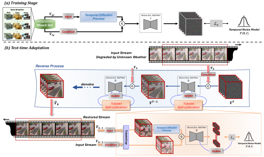
Figure 3: Overview of our Diff-TTA framework for video adverse weather removal. In the training stage, through the temporal diffusion process, we randomly add temporal noise on the clean video clip $\mathbf{V}_{gt}$ from the mixed training set. Then, the denoising NAFNet $\epsilon_{\theta}$ is trained by estimating the applied noise, which is conditioned by the degraded counterpart $\mathbf{V}_{lq}$ by seen weather types. In the test stage, the proxy task, Diff-TSC, where the cropped tubelets of the last restored pair $\{\mathbf{V}_{k-1},\hat{\mathbf{V}}_{k-1}\}$ are utilized to learn the primer distribution, is incorporated into each timestep of denoising the randomly sampled temporal noise $\mathbf{V}^{T}_{k}$ for the iterative online adaptation.

In this work, we devise the first diffusion-based model to remove arbitrary adverse weather in videos with one set of model parameters. We follow an end-to-end formulation of video adverse weather removal, which reads:

$$\hat{\mathbf{V}}_{k}=\phi(\textbf{V}_{k}),\mathbf{V}_{k}=\{I_{i}\}_{i=1}^{N_{f}},$$ (2)

where $\textbf{V}_{k}$ is the $k$-th video clip with $N_{f}$ frames degraded by arbitrary weather type, $\hat{\mathbf{V}}_{k}$ is the restored clip. $\phi$ is the denoising function derived from DDIM [38]. The denoising network $\epsilon_{\theta}$ in the denoising function consists of a single encoder and decoder.

In the training stage, we follow the formulation of DDIM and extend the diffusion forward process to a temporal counterpart for frame-correlation modeling. The denoising network $\epsilon_{\theta}$ with NAFNet [6] as the backbone is trained for noise estimation, which enforces the output of the model to approximate the proposed temporal noise model. During the inference stage, we present a proxy task, Diff-TSC, to adapt the diffusion model to the target test data degraded by unknown weather based on the diffusion reverse process. We iteratively optimize the noise estimation of the cropped tubelets and calibrate the weight set of the model parameters for more robust weather removal. Next, we elaborate on our diffusion-based solution for adverse weather removal in videos and our diffusion test-time adaptation, which are also displayed in Figure 3.

4.1 Temporal Diffusion Process

The traditional diffusion model is trained to denoise independent noise from a perturbed image. The noise $\epsilon$ in Eq. (1) is sampled from an i.i.d. Gaussian distribution $\epsilon\sim\mathcal{N}(0,\mathbf{I})$. Upon training the image diffusion model and utilizing it to reverse frames from a video into the noise space individually, the significant correlation among the noise maps of these frames can be easily observed. Rather than introducing massive parameters into the denoising network, we extend the original diffusion process to the temporal counterpart by an ARMA-based temporal noise model to efficiently preserve the correlation between frames.

Temporal noise model. ARMA (Auto-regressive Moving Average) [2] is a widely used statistical model for time series data, which combines the auto-regressive (AR) part and the moving average (MA) part. Typically, ARMA can be formulated as:

$$X_{t}=c+\varepsilon_{t}+\sum_{i=1}^{p}\varphi_{i}X_{t-i}+\sum_{j=1}^{q}\tau_{j}\varepsilon_{t-j},$$ (3)

where $X$ is the value term, $\varepsilon$ is the error term, $c$ is a constant term, $p,q$ are the auto-regressive order and moving average order while $\varphi,\tau$ are their coefficients, respectively. Motivated by ARMA, we develop the original Gaussian noise model $\mathcal{N}(0,\mathbf{I})$ to the temporal noise model $\mathcal{T}(0,\mathbf{I})$. Specifically, let $\{\bar{\epsilon}_{i}\}_{i=1}^{N_{f}}$ denote the noise sequence corresponding to consecutive frames of a video clip. We first sample the noise sequence $\{\bar{\epsilon}_{i}\}_{i=1}^{N_{f}}$ and the corresponding error sequence $\{\varepsilon_{i}\}_{i=1}^{N_{f}}$ from $\mathcal{N}(0,\mathbf{I})$, respectively. The constant term $c$ should be consistent with the mean of Gaussian distribution, that is, zero. To take both the past and future information into consideration, we enforce the noise of the current frame affected not only by the noise and error term of the previous frame but also those of the next frame, and correspondingly the auto-regressive order and moving average order $p,q=1$. Consequently, the expression in Eq. (3) evolves into the convex combination of the noise term and error term:

$$\bar{\epsilon}_{i}=(1-\varphi-\tau)\varepsilon_{i}+\varphi\frac{\bar{\epsilon}_{i-1}+\bar{\epsilon}_{i+1}}{2}+\tau\frac{\varepsilon_{i-1}+\varepsilon_{i+1}}{2},$$ (4)

where $\varphi,\tau$ are empirically set as $0.6,0.3$, respectively. Algorithm 1 further illustrates our temporal noise model, where the noise sequence of each video clip is constructed with separate preorder and postorder steps.

Input: $K$ clips: $\{\mathbf{V}_{1},\mathbf{V}_{2},\ldots,\mathbf{V}_{K}\}$ in a batch; The coefficients $\varphi,\tau$

1

2for Clip $k=1,2,...,K$ parallelly do

3       for Frame $i=1,2,...,N_{f}$ parallelly do

4             sample $\bar{\epsilon}_{i},\varepsilon_{i}\in\mathbb{R}^{1\times c\times h\times w}$ from $\mathcal{N}(0,\mathbf{I})$

5            

6       end for

7      for Frame $i=2,3,...,N_{f}$ sequentially do

8             $\bar{\epsilon}_{i}=(1-\varphi-\tau)\varepsilon_{i}+\varphi\bar{\epsilon}_{i-1}+\tau\varepsilon_{i-1}$

9            

10       end for

11      for Frame $i=N_{f}-1,...,2,1$ sequentially do

12             $\bar{\epsilon}_{i}=(1-\varphi-\tau)\varepsilon_{i}+\varphi\bar{\epsilon}_{i+1}+\tau\varepsilon_{i+1}$

13            

14       end for

15      $\bar{\epsilon}=normalize(\bar{\epsilon})\Longrightarrow\bar{\epsilon}\sim\mathcal{T}(0,\mathbf{I})$

16 end for

17Return $\{\{\bar{\epsilon_{i}}|\bar{\epsilon_{i}}\in\mathbb{R}^{1\times c\times h\times w}\}_{i=1}^{N_{f}}\}_{k=1}^{K}$

Algorithm 1 Temporal Noise Model $\mathcal{T}(0,\mathbf{I})$

To enhance the capacity of our denoising network for capturing temporal dependencies, we have specifically modified the architecture by substituting only the first and last layers of the denoising NAFNet with the 3D convolutional layer. This tailored network, denoted as $\epsilon_{\theta}$ is then optimized as:

$$\mathcal{L}_{S}=\|\bar{\epsilon}-\epsilon_{\theta}(\sqrt{\bar{\alpha}_{t}}\hat{\mathbf{V}}+\sqrt{1-\bar{\alpha_{t}}}\bar{\epsilon},\mathbf{V},t)\|_{1},\\$$ (5)

where we utilize the temporal noise model as the supervision, and $\|\cdot\|$ denotes $L_{1}$ norm.

4.2 Diffusion Test-time Adaptation

Once trained by the proposed temporal noise model, the network $\epsilon_{\theta}$ can generate high-quality images. This is achieved by sampling a noisy state $\mathbf{V}_{T}$ and then iteratively denoising it in the reverse process. Yang et al. [52] introduced adversarial learning for weather conditions, which require weather type annotations during the training stage. Additionally, their method may fail to address out-of-distribution data, because including all real-world conditions in training, considering both weather types and image statistics, is impractical. Contrastively, we introduce test-time adaptation and update knowledge by practice to remove arbitrary weather conditions robustly. We design and incorporate Diffusion Tubelet Self-Calibration (Diff-TSC), a proxy task, into the iterative denoising of the diffusion reverse process to learn the primer distribution of the frames degraded by unknown weather.

Table 1: Quantitative evaluation on seen weather conditions for video adverse weather removal. For Original Weather, these methods are trained on the weather-specific training set and tested on the weather-specific testing set. For Rain, Haze, and Snow, these methods are trained on a mixed training set and tested on the weather-specific testing set. The average performance is calculated on Rain, Haze, and Snow. PSNR and SSIM are adopted as our evaluation metrics. The best and second-best values are bold and underlined.

Methods		Type	Source	Datasets
				Original Weather		Rain		Haze		Snow		Average
Derain	PReNet [35]	Image	CVPR’19	27.06	0.9077	26.80	0.8814	17.64	0.8030	28.57	0.9401	24.34	0.8748
	SLDNet [51]	Video	CVPR’20	20.31	0.6272	21.24	0.7129	16.21	0.7561	22.01	0.8550	19.82	0.7747
	S2VD [55]	Video	CVPR’21	24.09	0.7944	28.39	0.9006	19.65	0.8607	26.23	0.9190	24.76	0.8934
	RDD-Net [43]	Video	ECCV’22	31.82	0.9423	30.34	0.9300	18.36	0.8432	30.40	0.9560	26.37	0.9097
Dehaze	GDN [26]	Image	ICCV’19	19.69	0.8545	29.96	0.9370	19.01	0.8805	31.02	0.9518	26.66	0.9231
	MSBDN [15]	Image	CVPR’20	22.01	0.8759	26.70	0.9146	22.24	0.9047	27.07	0.9340	25.34	0.9178
	VDHNet [36]	Video	TIP’19	16.64	0.8133	29.87	0.9272	16.85	0.8214	29.53	0.9395	25.42	0.8960
	PM-Net [28]	Video	MM’22	23.83	0.8950	25.79	0.8880	23.57	0.9143	18.71	0.7881	22.69	0.8635
Desnow	DesnowNet [29]	Image	TIP’18	28.30	0.9530	25.19	0.8786	16.43	0.7902	27.56	0.9181	23.06	0.8623
	DDMSNET [58]	Image	TIP’21	32.55	0.9613	29.01	0.9188	19.50	0.8615	32.43	0.9694	26.98	0.9166
	HDCW-Net [10]	Image	ICCV’21	31.77	0.9542	28.10	0.9055	17.36	0.7921	31.05	0.9482	25.50	0.8819
	SMGARN [13]	Image	TCSVT‘22	33.24	0.9721	27.78	0.9100	17.85	0.8075	32.34	0.9668	25.99	0.8948
Restoration	MPRNet [56]	Image	CVPR’21	— —	— —	28.22	0.9165	20.25	0.8934	30.95	0.9482	26.47	0.9194
	EDVR [44]	Video	CVPR’19	— —	— —	31.10	0.9371	19.67	0.8724	30.27	0.9440	27.01	0.9178
	RVRT [23]	Video	NIPS’22	— —	— —	30.11	0.9132	21.16	0.8949	26.78	0.8834	26.02	0.8972
	RTA [63]	Video	CVPR’22	— —	— —	30.12	0.9186	20.75	0.8915	29.79	0.9367	26.89	0.9156
Multi-Weather	All-in-one [21]	Image	CVPR‘20	— —	— —	26.62	0.8948	20.88	0.9010	30.09	0.9431	25.86	0.9130
	UVRNet [19]	Image	TMM’22	— —	— —	22.31	0.7678	20.82	0.8575	24.71	0.8873	22.61	0.8375
	TransWeather [39]	Image	CVPR’22	— —	— —	26.82	0.9118	22.17	0.9025	28.87	0.9313	25.95	0.9152
	TKL [11]	Image	CVPR’22	— —	— —	26.73	0.8935	22.08	0.9044	31.35	0.9515	26.72	0.9165
	WeatherDiffusion [34]	Image	TPAMI’23	— —	— —	25.86	0.9125	20.10	0.8442	26.40	0.9113	24.12	0.8893
	WGWS-Net [64]	Image	CVPR’23	— —	— —	29,64	0.9310	17.71	0.8113	31.58	0.9528	26.31	0.9265
	ViWS-Net [52]	Video	ICCV’23	— —	— —	31.52	0.9433	24.51	0.9187	31.49	0.9562	29.17	0.9394
	Ours	Video	— —	— —	— —	32.43	0.9573	24.56	0.9148	31.86	0.9640	29.63	0.9453

Input: $K$ overlapped clips: $\{\mathbf{V}_{1},\mathbf{V}_{2},\ldots,\mathbf{V}_{K}\}$ in one video stream

1 for Clip $k=1,2,...,K$ sequentially do

2       Initialize the network $\epsilon_{\bar{\theta}}$ with $\theta$

3       Initialize $\hat{\mathbf{V}}_{k}$ by Algorithm 1

4       if $k=1$ then

5             for step $t=T,\ldots,2,1$ sequentially do

6                  $\hat{\mathbf{V}}_{k}=ddim(\mathbf{V}_{k},\hat{\mathbf{V}}_{k},\epsilon_{\bar{\theta}},t)$

7             end for

8            

9      else

10             $\mathbf{A},\hat{\mathbf{A}}=TubeletCrop(\mathbf{V}_{k-1},\hat{\mathbf{V}}_{k-1},N_{a})$

11            

12            for step $t=T,\ldots,2,1$ sequentially do

13                   Compute $\mathcal{L}_{S}(\mathbf{A},\hat{\mathbf{A}},\bar{\epsilon},t)$ by Eq. (5)

14                   $\bar{\theta}=\bar{\theta}-\delta\bigtriangledown_{\bar{\theta}}\mathcal{L}_{S}$

15                   $\hat{\mathbf{V}}_{k}=ddim(\mathbf{V}_{k},\hat{\mathbf{V}}_{k},\epsilon_{\bar{\theta}},t)$

16             end for

17            $\hat{\mathbf{V}}_{k}=integrate(\hat{\mathbf{V}}_{k},\hat{\mathbf{V}}_{k-1})$

18            

19       end if

20      

21 end for

22Return the restored clips$\{\hat{\mathbf{V}}_{1},\hat{\mathbf{V}}_{2},...,\hat{\mathbf{V}}_{K}\}$

23

Algorithm 2 Diffusion Test-Time Adaptation to unknown weather. $\theta$ is the weight set of the trained network before adaptation, $\delta$ is the learning rate for online adaptation.

Diffusion Tubelet Self-Calibration. We design a proxy task for self-supervised learning to transfer the diffusion model to the specific weather condition. Specifically, for each clip from the video stream, we first initialize the weight set of $\epsilon_{\bar{\theta}}$ with $\theta$ trained by source data. We leverage the previous clip $\mathbf{V}_{k-1}$ and its restored result $\hat{\mathbf{V}}_{k-1}$ as the pair of condition and input for the online optimization when inferring the current clip $\mathbf{V}_{k}$. Rather than directly traversing all fine-grained details, we randomly crop $N_{a}$ tubelets from $\mathbf{V}_{k-1}$ as the primer distribution to avoid memory overhead and massive computational costs caused by high resolution. Following the process in Section 4.1, we conduct our temporal diffusion process on the restored tubelets $\hat{\mathbf{A}}$ and feed them together with the degraded tubelets $\mathbf{A}$ into the denoising NAFNet for noise estimation. As suggested in [41], it is necessary to iteratively find a relatively optimal point for the target distribution during test-time adaptation. Inherited from the characteristics of DDIM, such requirement can be easily achieved in the iterative diffusion reverse process, which needs more increments of inference time in the traditional CNNs and Transformers. For each timestep $t$, we first obtain the noisy tubelet $\hat{\mathbf{A}}_{t}$ and then optimize the objective function given in Eq. (5) to update the weight set $\bar{\theta}$. After the iterative adaptation to $\hat{\mathbf{V}}_{k}$, we ensemble the overlapped part of it with that of the previous clip $\hat{\mathbf{V}}_{k-1}$ to capture complementary information of pre-adaptation and post-adaptation. We optimize over the entire network except for the last layer suggested by SHOT [22]. The detailed procedure is described in Algorithm 2. We emphasize the synergy between diffusion models and test-time adaptation in accumulating frame-correlated knowledge for adverse weather removal. By attaching the proxy task to iterative denoising, our approach also avoids excessive computational overhead caused by iterative adaptation.

5 Experiments

Table 2: Quantitative evaluation on unseen weather conditions for video adverse weather removal. The best and second-best performances are marked in bold and underlined, respectively.

Method	VRDS [45]		RVSD [4]
	PSNR $\uparrow$	SSIM $\uparrow$	PSNR $\uparrow$	SSIM $\uparrow$
All-in-one [21]	20.44	0.5944	19.79	0.7509
TransWeather [39]	21.36	0.7136	20.25	0.7514
TKL [11]	20.49	0.7003	19.71	0.7370
WeatherDiffusion [34]	20.73	0.6943	18.08	0.6588
ViWS-Net [52]	21.57	0.7094	19.83	0.7590
Diff-TTA (ours)	22.57	0.7281	22.35	0.7719

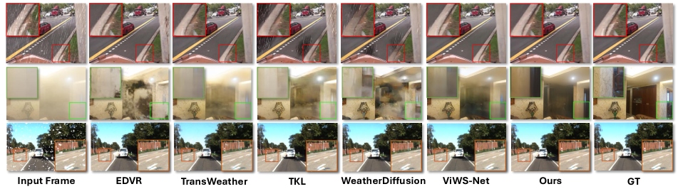
Figure 4: Qualitative Comparison of seen weather conditions between our approach and state-of-the-art algorithms. The competitive algorithms are selected to present the results on the example frames degraded by rain, haze, snow, respectively. The color box indicates the comparison of details. Please zoom in on the images for improved visualization.

5.1 Datasets

Various video adverse weather datasets are used in our experiments. Following the setting of [52], we adopt RainMotion [43], REVIDE [61] and KITTI-snow [52] as seen weather. For the training stage, we merge the training set of the three datasets as the mixed set to learn a generic model. For the testing stage, we evaluate our model on three testing sets, respectively. Additionally, we evaluate our approach on two datasets VRDS [45] and RVSD [4] to validate the generalization of our Diff-TTA on unseen weather conditions. VRDS is a synthesized video dataset of joint rain streaks and raindrops with a total of 102 videos, while RVSD is a realistic video desnowing dataset with a total of 110 videos containing both snow and fog achieved by the rendering engine. Due to the large quantity of the two datasets, we randomly sample 8 videos as the test set, each of which has 20 frames, respectively. We also collect several real-world videos degraded by diverse weather conditions to prove its effectiveness on real-world applications.

5.2 Implementation

Training Details. The proposed framework was trained on NVIDIA RTX 4090 GPUs and implemented on the Pytorch platform. We adopted the Lion optimizer [12] ($\beta_{1}=0.9,\beta_{2}=0.99$) with the initial learning rate of $2\times 10^{-5}$ decayed to $2\times 10^{-7}$ by the Cosine scheduler. We randomly crop the video frames to 256$\times$256 for training. Our framework is empirically trained for 600k iterations in an end-to-end way with batch size of 4. Each batch consists of 4 video clips with 5 frames per clip.

Method-specific Details. During the training, we used the diffusion process linearly increasing from $\beta_{1}=0.0001$ to $\beta_{T}=0.02$ with $T=1000$ timesteps. During the testing, the inference step is reduced to 25 by deterministic implicit sampling. We utilize the same optimizer with a smaller learning rate of $1\times 10^{-6}$ for the test-time adaptation. The number of cropped tubelets $N_{a}$ is empirically set to 5 while the crop size is 128$\times$128. Despite the incorporated adaptation, our Diff-TTA is particularly 90$\times$ more efficient than WeatherDiffusion. To process a video clip of 5 frames with the patch size of 256$\times$256, the average run time of Diff-TTA is 6.01s while that of WeatherDiffusion is 542.76s.

5.3 Performance Evaluation

Comparison methods. As shown in Table 1, we compared our proposed method against five kinds of state-of-the-art methods on the three seen weather conditions as [52] does, i.e., derain, dehaze, desnow, restoration, all-in-one adverse weather removal. For all-in-one adverse weather removal, we compared ours with the six representative single-image methods All-in-one [21], UVRNet [19], TransWeather [39], TKL [11], WeatherDiffusion [34], WGWS-Net [64], and the video-level method ViWS-Net [52].

Table 3: Ablation study of each critical component in the proposed framework on seen weather conditions. The top values are marked in bold font. “Diff-TTA” denote Diffusion Test-time Adaptation.

Combination	Component			Datasets
	Diffusion Process	Temporal Noise	Diff-TTA	Rain		Haze		Snow		Average
M1	-	-	-	29.07	0.9514	22.64	0.8930	28.79	0.9350	26.83	0.9264
M2	✓	-	-	31.55	0.9466	23.58	0.9041	30.48	0.9520	28.52	0.9342
M3	✓	✓	-	32.10	0.9530	24.31	0.9124	31.04	0.9621	29.15	0.9425
Ours	✓	✓	✓	32.43	0.9573	24.56	0.9148	31.86	0.9640	29.63	0.9453

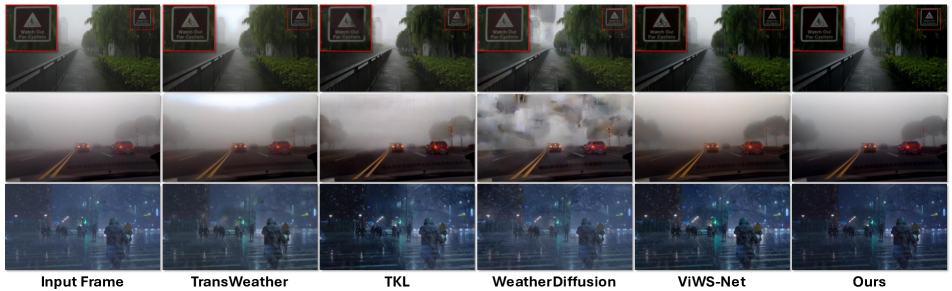
Figure 5: Visual comparison of all-in-one adverse weather removal methods on the selected real-world video sequences degraded by rain, haze, snow. Apparently, our network can more effectively remove rain streaks, haze, and snowflakes of input video frames than state-of-the-art methods. Please zoom in on the images for improved visualization.

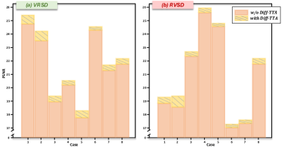
Figure 6: Detailed results on each case of VRDS and RVSD by our proposed Diff-TTA. The proposed Diff-TTA brings consistent improvement across various cases.

Quantitative Comparison. For quantitative evaluation of the restored results, we apply the peak signal-to-noise ratio (PSNR) and the structural similarity (SSIM) as the metrics. Following the previous experimental setting, only the results of the model trained on the mixed training set are reported for all-in-one adverse weather removal models. To ensure the fairness of comparisons, we retrain each compared model implemented by the official codes based on our training dataset and report the best result. Observed from Table 1, our method achieves the best average performance across rain, haze and snow conditions among all kinds of methods by a considerable margin of 0.46, 0.0059 in PSNR, SSIM, respectively, than the second-best method ViWS-Net [52]. Though some single-weather methods like DDMSNET [58] and SMGARN [13] achieve impressive results in their own weather condition, they frequently fail to remove other weather conditions, such as haze. Our method significantly surpasses other all-in-one adverse weather methods in rain and snow conditions, and obtains competitive results in haze conditions. It is worth noting that the generalizable ability is critical for such methods, which can be observed from the average performance. To further validate their generalization, we evaluate all-in-on adverse weather removal methods on unseen weather conditions, i.e., rain streak+raindrop and snow+fog, in Table 2. Our Diff-TTA exhibits remarkable superiority over state-of-the-art methods when confronted with these unseen weather conditions.

Visual comparisons on synthetic videos. To vividly demonstrate the effectiveness of our approach, Figure 4 shows the qualitative comparison under the rain, haze, and snow conditions between our method and five state-of-the-art methods Our method demonstrates promising results in terms of visual quality across various weather types. Specifically, when it comes to rain and snow scenarios, our approach significantly reduces the presence of rain streaks and snow particles, outperforming other methods. In hazy scenarios, our method effectively removes residual haze and preserves the clean background with impressive results. More visual results of seen and unseen weather are displayed in the supplementary files.

Visual comparisons on real-world videos. To evaluate the universality of our Diff-TTA on real-world applications, we collect several real-world degraded videos by rain, haze, snow from Youtube website, and further compare our approach against other all-in-one adverse weather removal methods. Figure 5 displays the visual results produced by our network and the compared methods on real-world video frames, clearly showcasing our exceptional performance.

Ablation Study. We evaluate the effectiveness of each component including diffusion process, temporal noise model, and Diffusion test-time adaptation (Diff-TTA) as described in Table 3. We present the results trained on the mixed training set and tested on three weather-specific testing sets (rain, haze, snow) in view of PSNR and SSIM. The baseline model M1, i.e., the vanilla NAFNet, achieves the average performance on the three adverse weather datasets of 26.83, 0.9264 in PSNR, SSIM, respectively. M2 is equipped with diffusion process and trained by noise estimation, which advances M1 on the average performance by 1.69, 0.0078 of PSNR, SSIM, respectively. M3 introduces the proposed temporal noise model by replacing the vanilla noise model, and brings about an improvement of 0.63, 0.0083 in average PSNR, SSIM, respectively. Finally, our full model employs diffusion test-time adaptation (Diff-TTA) and gains a critical increase of 0.48, 0.0028 in PSNR, SSIM, respectively, compared to M3. Figure 6 further ablates our iterative adaptation on each case of the two unseen datasets, demonstrating consistent improvements.

6 Conclusion

This paper presents Diff-TTA, a diffusion-based test-time adaptation method capable of restoring videos degraded by various, even unknown, weather conditions. The proposed approach involves constructing a diffusion-based network and utilizing a novel temporal noise model to establish correlations among video frames. More importantly, a proxy task Diff-TSC is incorporated into the diffusion reverse process to iteratively update the deep model. This allows for the efficient adaptation of vision systems in real-world scenarios without modifying the source training process, making it easily applicable to a wide range of off-the-shelf diffusion-based models for enhancing weather removal. Experimental results on both synthetic and real-world data, which encompass diverse weather conditions, confirm the effectiveness and generalization capability of the proposed approach. We believe Diff-TTA can be a compelling baseline that shifts the focus of the community from the complicated training process to online test-time adaptation.

Supplementary Material

This is a supplementary material for Genuine Knowledge from Practice: Diffusion Test-Time Adaptation for Video Adverse Weather Removal.

We provide the following materials in this manuscript:

• Sec. 7 more details of our designed method.

• Sec. 8 computational costs comparison.

• Sec. 9 visualization results

• Sec. 10 future work

7 More Details

In our proposed method, we adopt NAFNet [6] as the backbone of the denoising network. NAFNet is a very simple but efficient baseline for image restoration task. We adapt it to video restoration tasks based on its original setting. Specifically, it is enlarged by increasing the width to 64, the number of blocks of NAFNet to 44. The additional MLP layer comprised of SimpleGate and a linear layer is incorporated into each block for time embedding as shown in Figure 7.

8 Computational Costs Comparison

In this section, we showcase our speed advantages against diffusion-based restoration methods. We conduct all inference stages on an RTX4090 GPU to ensure a fair comparison. The results of FLOPs and run-time on a video clip of 5 frames with 256$\times$256 patch size are displayed in Table 4. This demonstrates that our approach achieves superior model complexity and run-time performance after incorporating the adaptation mechanism while obtaining promising restoration performance.

9 More Visualization Results

We present more visual comparisons against state-of-the-art methods on synthetic and real datasets to demonstrate the excellent visual performance and generalization ability of Diff-TTA in removing arbitrary adverse weather conditions. The restored results of consecutive frames with diverse weather conditions are also displayed in the supplementary videos.

Visualization comparison on seen datasets. We provide more qualitative comparisons between our Diff-TTA and SOTA methods. The results are shown in Figure 8. Our Diff-TTA achieves the best visual quality by removing adverse components and recovering more background details.

Visualization comparison on unseen datasets. We provide qualitative comparisons between our Diff-TTA and SOTA methods. The results are shown in Figure 9, 10. Our Diff-TTA achieves the best visual quality by removing unknown adverse components and recovering more background details.

Visualization comparison on real-world data. We provide more qualitative comparisons between our Diff-TTA and SOTA methods. The results are shown in Figure 11. Our Diff-TTA achieves the best visual quality by removing unknown adverse components and recovering more background details, further validating its generalization.

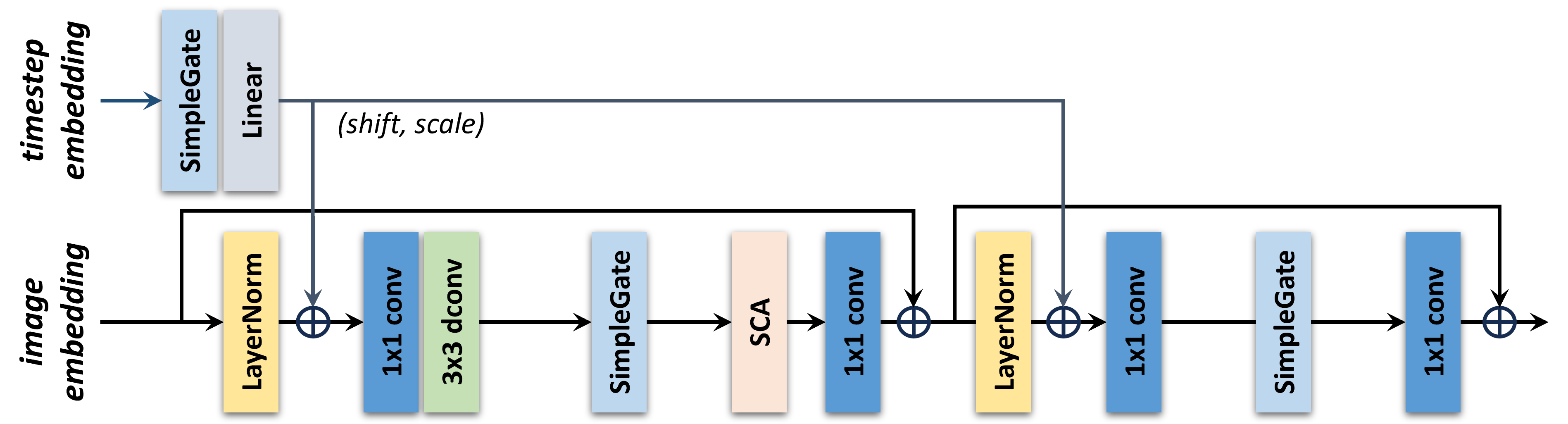
Figure 7: Detailed structure of the Denoising NAFNet’s block.

Table 4: Comparison of FLOPs and Run-time on a video clip of 5 frames with 256$\times$256 patch size.

Method	IR-SDE [30]	Refusion [31]	WeatherDiffusion [34]	Diff-TTA(ours)
FLOPs/G	1896.67$\times$100 steps	372.38$\times$100 steps	1242.01$\times$1000 steps	385.14$\times$25 steps
Run-time/s	23.42	12.55	542.76	6.01

10 Future Work

In the future, we plan further to accelerate the inference speed of Diff-TTA for real-time applications. Additionally, we will apply test-time adaptation to other restoration tasks.

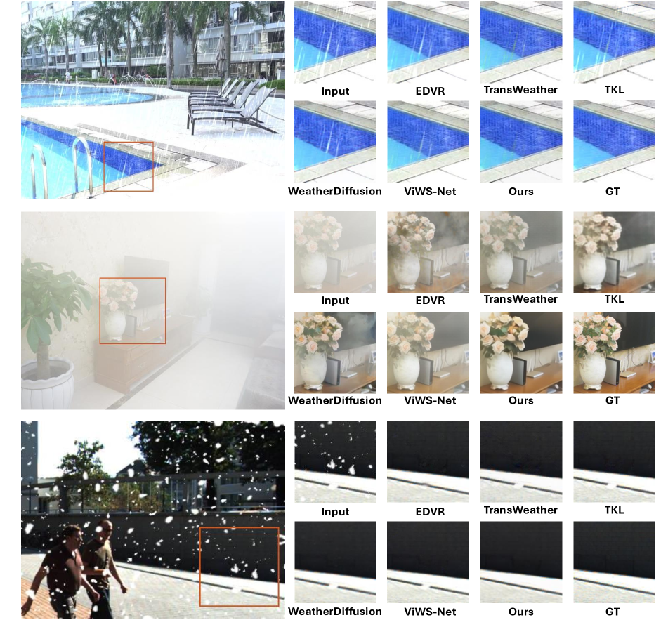
Figure 8: More visual comparisons on seen weather conditions.

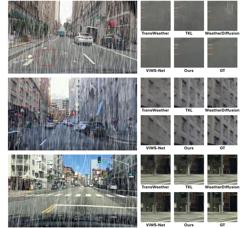
Figure 9: More visual comparisons on unseen weather conditions.

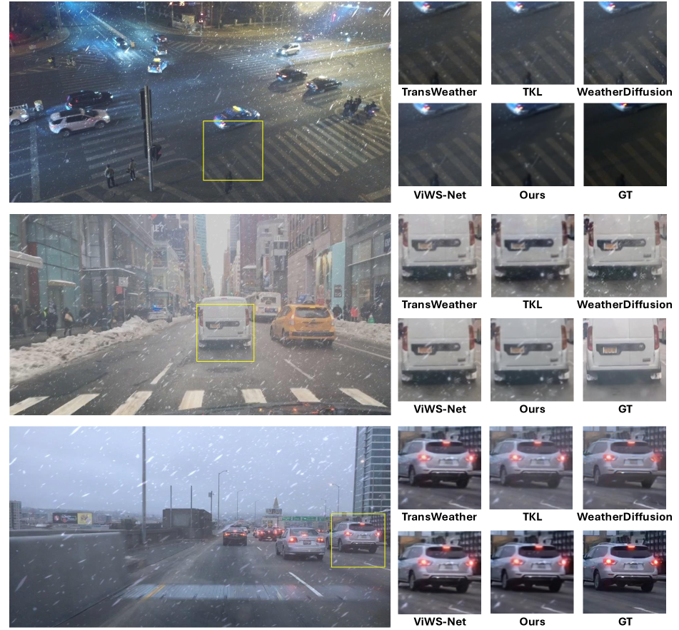
Figure 10: More visual comparisons on unseen weather conditions.

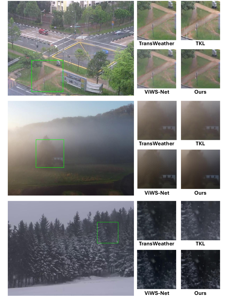
Figure 11: More visual comparisons on real-world scenarios.

References

- Boudiaf et al. [2022] Malik Boudiaf, Romain Mueller, Ismail Ben Ayed, and Luca Bertinetto. Parameter-free online test-time adaptation. In Proceedings of the IEEE/CVF Conference on Computer Vision and Pattern Recognition, pages 8344–8353, 2022.
- Box [2013] George Box. Box and jenkins: time series analysis, forecasting and control. In A Very British Affair: Six Britons and the Development of Time Series Analysis During the 20th Century, pages 161–215. Springer, 2013.
- Chen et al. [2022a] Dian Chen, Dequan Wang, Trevor Darrell, and Sayna Ebrahimi. Contrastive test-time adaptation. In Proceedings of the IEEE/CVF Conference on Computer Vision and Pattern Recognition, pages 295–305, 2022a.
- Chen et al. [2023a] Haoyu Chen, Jingjing Ren, Jinjin Gu, Hongtao Wu, Xuequan Lu, Haoming Cai, and Lei Zhu. Snow removal in video: A new dataset and a novel method. In Proceedings of the IEEE/CVF International Conference on Computer Vision, pages 13211–13222, 2023a.
- Chen et al. [2018] Jie Chen, Cheen-Hau Tan, Junhui Hou, Lap-Pui Chau, and He Li. Robust video content alignment and compensation for rain removal in a cnn framework. In Proceedings of the IEEE conference on computer vision and pattern recognition, pages 6286–6295, 2018.
- Chen et al. [2022b] Liangyu Chen, Xiaojie Chu, Xiangyu Zhang, and Jian Sun. Simple baselines for image restoration. In European Conference on Computer Vision, pages 17–33. Springer, 2022b.
- Chen et al. [2023b] Sixiang Chen, Tian Ye, Yun Liu, Jinbin Bai, Haoyu Chen, Yunlong Lin, Jun Shi, and Erkang Chen. Cplformer: Cross-scale prototype learning transformer for image snow removal. In Proceedings of the 31st ACM International Conference on Multimedia, pages 4228–4239, 2023b.
- Chen et al. [2023c] Sixiang Chen, Tian Ye, Chenghao Xue, Haoyu Chen, Yun Liu, Erkang Chen, and Lei Zhu. Uncertainty-driven dynamic degradation perceiving and background modeling for efficient single image desnowing. In Proceedings of the 31st ACM International Conference on Multimedia, pages 4269–4280, 2023c.
- Chen et al. [2020] Wei-Ting Chen, Hao-Yu Fang, Jian-Jiun Ding, Cheng-Che Tsai, and Sy-Yen Kuo. Jstasr: Joint size and transparency-aware snow removal algorithm based on modified partial convolution and veiling effect removal. In European Conference on Computer Vision, pages 754–770. Springer, 2020.
- Chen et al. [2021] Wei-Ting Chen, Hao-Yu Fang, Cheng-Lin Hsieh, Cheng-Che Tsai, I Chen, Jian-Jiun Ding, Sy-Yen Kuo, et al. All snow removed: Single image desnowing algorithm using hierarchical dual-tree complex wavelet representation and contradict channel loss. In Proceedings of the IEEE/CVF International Conference on Computer Vision, pages 4196–4205, 2021.
- Chen et al. [2022c] Wei-Ting Chen, Zhi-Kai Huang, Cheng-Che Tsai, Hao-Hsiang Yang, Jian-Jiun Ding, and Sy-Yen Kuo. Learning multiple adverse weather removal via two-stage knowledge learning and multi-contrastive regularization: Toward a unified model. In Proceedings of the IEEE/CVF Conference on Computer Vision and Pattern Recognition, pages 17653–17662, 2022c.
- Chen et al. [2023d] Xiangning Chen, Chen Liang, Da Huang, Esteban Real, Kaiyuan Wang, Yao Liu, Hieu Pham, Xuanyi Dong, Thang Luong, Cho-Jui Hsieh, et al. Symbolic discovery of optimization algorithms. arXiv preprint arXiv:2302.06675, 2023d.
- Cheng et al. [2022] Bodong Cheng, Juncheng Li, Ying Chen, Shuyi Zhang, and Tieyong Zeng. Snow mask guided adaptive residual network for image snow removal. arXiv preprint arXiv:2207.04754, 2022.
- Dhariwal and Nichol [2021] Prafulla Dhariwal and Alexander Nichol. Diffusion models beat gans on image synthesis. Advances in Neural Information Processing Systems, 34:8780–8794, 2021.
- Dong et al. [2020] Hang Dong, Jinshan Pan, Lei Xiang, Zhe Hu, Xinyi Zhang, Fei Wang, and Ming-Hsuan Yang. Multi-scale boosted dehazing network with dense feature fusion. In Proceedings of the IEEE/CVF conference on computer vision and pattern recognition, pages 2157–2167, 2020.
- Ho et al. [2020] Jonathan Ho, Ajay Jain, and Pieter Abbeel. Denoising diffusion probabilistic models. Advances in neural information processing systems, 33:6840–6851, 2020.
- Hu et al. [2021] Minhao Hu, Tao Song, Yujun Gu, Xiangde Luo, Jieneng Chen, Yinan Chen, Ya Zhang, and Shaoting Zhang. Fully test-time adaptation for image segmentation. In Medical Image Computing and Computer Assisted Intervention–MICCAI 2021: 24th International Conference, Strasbourg, France, September 27–October 1, 2021, Proceedings, Part III 24, pages 251–260. Springer, 2021.
- Iwasawa and Matsuo [2021] Yusuke Iwasawa and Yutaka Matsuo. Test-time classifier adjustment module for model-agnostic domain generalization. Advances in Neural Information Processing Systems, 34:2427–2440, 2021.
- Kulkarni et al. [2022] Ashutosh Kulkarni, Prashant W Patil, Subrahmanyam Murala, and Sunil Gupta. Unified multi-weather visibility restoration. IEEE Transactions on Multimedia, 2022.
- Li et al. [2018] Minghan Li, Qi Xie, Qian Zhao, Wei Wei, Shuhang Gu, Jing Tao, and Deyu Meng. Video rain streak removal by multiscale convolutional sparse coding. In Proceedings of the IEEE conference on computer vision and pattern recognition, pages 6644–6653, 2018.
- Li et al. [2020] Ruoteng Li, Robby T Tan, and Loong-Fah Cheong. All in one bad weather removal using architectural search. In Proceedings of the IEEE/CVF conference on computer vision and pattern recognition, pages 3175–3185, 2020.
- Liang et al. [2020] Jian Liang, Dapeng Hu, and Jiashi Feng. Do we really need to access the source data? source hypothesis transfer for unsupervised domain adaptation. In International conference on machine learning, pages 6028–6039. PMLR, 2020.
- Liang et al. [2022] Jingyun Liang, Yuchen Fan, Xiaoyu Xiang, Rakesh Ranjan, Eddy Ilg, Simon Green, Jiezhang Cao, Kai Zhang, Radu Timofte, and Luc Van Gool. Recurrent video restoration transformer with guided deformable attention. arXiv preprint arXiv:2206.02146, 2022.
- Liu et al. [2018a] Jiaying Liu, Wenhan Yang, Shuai Yang, and Zongming Guo. Erase or fill? deep joint recurrent rain removal and reconstruction in videos. In Proceedings of the IEEE conference on computer vision and pattern recognition, pages 3233–3242, 2018a.
- Liu et al. [2022a] Quande Liu, Cheng Chen, Qi Dou, and Pheng-Ann Heng. Single-domain generalization in medical image segmentation via test-time adaptation from shape dictionary. In Proceedings of the AAAI Conference on Artificial Intelligence, pages 1756–1764, 2022a.
- Liu et al. [2019] Xiaohong Liu, Yongrui Ma, Zhihao Shi, and Jun Chen. Griddehazenet: Attention-based multi-scale network for image dehazing. In Proceedings of the IEEE/CVF international conference on computer vision, pages 7314–7323, 2019.
- Liu et al. [2023] Xihui Liu, Dong Huk Park, Samaneh Azadi, Gong Zhang, Arman Chopikyan, Yuxiao Hu, Humphrey Shi, Anna Rohrbach, and Trevor Darrell. More control for free! image synthesis with semantic diffusion guidance. In Proceedings of the IEEE/CVF Winter Conference on Applications of Computer Vision, pages 289–299, 2023.
- Liu et al. [2022b] Ye Liu, Liang Wan, Huazhu Fu, Jing Qin, and Lei Zhu. Phase-based memory network for video dehazing. In Proceedings of the 30th ACM International Conference on Multimedia, pages 5427–5435, 2022b.
- Liu et al. [2018b] Yun-Fu Liu, Da-Wei Jaw, Shih-Chia Huang, and Jenq-Neng Hwang. Desnownet: Context-aware deep network for snow removal. IEEE Transactions on Image Processing, 27(6):3064–3073, 2018b.
- Luo et al. [2023a] Ziwei Luo, Fredrik K Gustafsson, Zheng Zhao, Jens Sjölund, and Thomas B Schön. Image restoration with mean-reverting stochastic differential equations. arXiv preprint arXiv:2301.11699, 2023a.
- Luo et al. [2023b] Ziwei Luo, Fredrik K Gustafsson, Zheng Zhao, Jens Sjölund, and Thomas B Schön. Refusion: Enabling large-size realistic image restoration with latent-space diffusion models. In Proceedings of the IEEE/CVF Conference on Computer Vision and Pattern Recognition, pages 1680–1691, 2023b.
- Nguyen et al. [2023] A Tuan Nguyen, Thanh Nguyen-Tang, Ser-Nam Lim, and Philip HS Torr. Tipi: Test time adaptation with transformation invariance. In Proceedings of the IEEE/CVF Conference on Computer Vision and Pattern Recognition, pages 24162–24171, 2023.
- Niu et al. [2022] Shuaicheng Niu, Jiaxiang Wu, Yifan Zhang, Yaofo Chen, Shijian Zheng, Peilin Zhao, and Mingkui Tan. Efficient test-time model adaptation without forgetting. In International conference on machine learning, pages 16888–16905. PMLR, 2022.
- Özdenizci and Legenstein [2023] Ozan Özdenizci and Robert Legenstein. Restoring vision in adverse weather conditions with patch-based denoising diffusion models. IEEE Transactions on Pattern Analysis and Machine Intelligence, 2023.
- Ren et al. [2019] Dongwei Ren, Wangmeng Zuo, Qinghua Hu, Pengfei Zhu, and Deyu Meng. Progressive image deraining networks: A better and simpler baseline. In Proceedings of the IEEE/CVF conference on computer vision and pattern recognition, pages 3937–3946, 2019.
- Ren et al. [2018] Wenqi Ren, Jingang Zhang, Xiangyu Xu, Lin Ma, Xiaochun Cao, Gaofeng Meng, and Wei Liu. Deep video dehazing with semantic segmentation. IEEE transactions on image processing, 28(4):1895–1908, 2018.
- Singh et al. [2022] Jaskirat Singh, Stephen Gould, and Liang Zheng. High-fidelity guided image synthesis with latent diffusion models. arXiv preprint arXiv:2211.17084, 2022.
- Song et al. [2020] Jiaming Song, Chenlin Meng, and Stefano Ermon. Denoising diffusion implicit models. arXiv preprint arXiv:2010.02502, 2020.
- Valanarasu et al. [2022] Jeya Maria Jose Valanarasu, Rajeev Yasarla, and Vishal M Patel. Transweather: Transformer-based restoration of images degraded by adverse weather conditions. In Proceedings of the IEEE/CVF Conference on Computer Vision and Pattern Recognition, pages 2353–2363, 2022.
- Van der Maaten and Hinton [2008] Laurens Van der Maaten and Geoffrey Hinton. Visualizing data using t-sne. Journal of machine learning research, 9(11), 2008.
- Wang et al. [2020] Dequan Wang, Evan Shelhamer, Shaoteng Liu, Bruno Olshausen, and Trevor Darrell. Tent: Fully test-time adaptation by entropy minimization. arXiv preprint arXiv:2006.10726, 2020.
- Wang et al. [2022a] Qin Wang, Olga Fink, Luc Van Gool, and Dengxin Dai. Continual test-time domain adaptation. In Proceedings of the IEEE/CVF Conference on Computer Vision and Pattern Recognition, pages 7201–7211, 2022a.
- Wang et al. [2022b] Shuai Wang, Lei Zhu, Huazhu Fu, Jing Qin, Carola-Bibiane Schönlieb, Wei Feng, and Song Wang. Rethinking video rain streak removal: A new synthesis model and a deraining network with video rain prior. In European Conference on Computer Vision, pages 565–582. Springer, 2022b.
- Wang et al. [2019] Xintao Wang, Kelvin CK Chan, Ke Yu, Chao Dong, and Chen Change Loy. Edvr: Video restoration with enhanced deformable convolutional networks. In Proceedings of the IEEE/CVF Conference on Computer Vision and Pattern Recognition Workshops, pages 0–0, 2019.
- Wu et al. [2023] Hongtao Wu, Yijun Yang, Haoyu Chen, Jingjing Ren, and Lei Zhu. Mask-guided progressive network for joint raindrop and rain streak removal in videos. In Proceedings of the 31st ACM International Conference on Multimedia, pages 7216–7225, 2023.
- Xia et al. [2023] Bin Xia, Yulun Zhang, Shiyin Wang, Yitong Wang, Xinglong Wu, Yapeng Tian, Wenming Yang, and Luc Van Gool. Diffir: Efficient diffusion model for image restoration. arXiv preprint arXiv:2303.09472, 2023.
- Xu et al. [2023] Jiaqi Xu, Xiaowei Hu, Lei Zhu, Qi Dou, Jifeng Dai, Yu Qiao, and Pheng-Ann Heng. Video dehazing via a multi-range temporal alignment network with physical prior. In Proceedings of the IEEE/CVF Conference on Computer Vision and Pattern Recognition, pages 18053–18062, 2023.
- Yan et al. [2021] Wending Yan, Robby T Tan, Wenhan Yang, and Dengxin Dai. Self-aligned video deraining with transmission-depth consistency. In Proceedings of the IEEE/CVF Conference on Computer Vision and Pattern Recognition, pages 11966–11976, 2021.
- Yang et al. [2022] Hongzheng Yang, Cheng Chen, Meirui Jiang, Quande Liu, Jianfeng Cao, Pheng Ann Heng, and Qi Dou. Dltta: Dynamic learning rate for test-time adaptation on cross-domain medical images. IEEE Transactions on Medical Imaging, 41(12):3575–3586, 2022.
- Yang et al. [2019] Wenhan Yang, Jiaying Liu, and Jiashi Feng. Frame-consistent recurrent video deraining with dual-level flow. In Proceedings of the IEEE/CVF Conference on Computer Vision and Pattern Recognition, pages 1661–1670, 2019.
- Yang et al. [2020] Wenhan Yang, Robby T Tan, Shiqi Wang, and Jiaying Liu. Self-learning video rain streak removal: When cyclic consistency meets temporal correspondence. In Proceedings of the IEEE/CVF Conference on Computer Vision and Pattern Recognition, pages 1720–1729, 2020.
- Yang et al. [2023a] Yijun Yang, Angelica I Aviles-Rivero, Huazhu Fu, Ye Liu, Weiming Wang, and Lei Zhu. Video adverse-weather-component suppression network via weather messenger and adversarial backpropagation. In Proceedings of the IEEE/CVF International Conference on Computer Vision, pages 13200–13210, 2023a.
- Yang et al. [2023b] Yijun Yang, Huazhu Fu, Angelica I Aviles-Rivero, Carola-Bibiane Schönlieb, and Lei Zhu. Diffmic: Dual-guidance diffusion network for medical image classification. In International Conference on Medical Image Computing and Computer-Assisted Intervention, pages 95–105. Springer, 2023b.
- Ye et al. [2023] Tian Ye, Sixiang Chen, Jinbin Bai, Jun Shi, Chenghao Xue, Jingxia Jiang, Junjie Yin, Erkang Chen, and Yun Liu. Adverse weather removal with codebook priors. In Proceedings of the IEEE/CVF International Conference on Computer Vision, pages 12653–12664, 2023.
- Yue et al. [2021] Zongsheng Yue, Jianwen Xie, Qian Zhao, and Deyu Meng. Semi-supervised video deraining with dynamical rain generator. In Proceedings of the IEEE/CVF Conference on Computer Vision and Pattern Recognition, pages 642–652, 2021.
- Zamir et al. [2021] Syed Waqas Zamir, Aditya Arora, Salman Khan, Munawar Hayat, Fahad Shahbaz Khan, Ming-Hsuan Yang, and Ling Shao. Multi-stage progressive image restoration. In Proceedings of the IEEE/CVF conference on computer vision and pattern recognition, pages 14821–14831, 2021.
- Zhang et al. [2023a] Jian Zhang, Lei Qi, Yinghuan Shi, and Yang Gao. Domainadaptor: A novel approach to test-time adaptation. In Proceedings of the IEEE/CVF International Conference on Computer Vision, pages 18971–18981, 2023a.
- Zhang et al. [2021a] Kaihao Zhang, Rongqing Li, Yanjiang Yu, Wenhan Luo, and Changsheng Li. Deep dense multi-scale network for snow removal using semantic and depth priors. IEEE Transactions on Image Processing, 30:7419–7431, 2021a.
- Zhang et al. [2023b] Lvmin Zhang, Anyi Rao, and Maneesh Agrawala. Adding conditional control to text-to-image diffusion models. In Proceedings of the IEEE/CVF International Conference on Computer Vision, pages 3836–3847, 2023b.
- Zhang et al. [2022] Marvin Zhang, Sergey Levine, and Chelsea Finn. Memo: Test time robustness via adaptation and augmentation. Advances in Neural Information Processing Systems, 35:38629–38642, 2022.
- Zhang et al. [2021b] Xinyi Zhang, Hang Dong, Jinshan Pan, Chao Zhu, Ying Tai, Chengjie Wang, Jilin Li, Feiyue Huang, and Fei Wang. Learning to restore hazy video: A new real-world dataset and a new method. In Proceedings of the IEEE/CVF Conference on Computer Vision and Pattern Recognition, pages 9239–9248, 2021b.
- Zhang et al. [2023c] Yi Zhang, Xiaoyu Shi, Dasong Li, Xiaogang Wang, Jian Wang, and Hongsheng Li. A unified conditional framework for diffusion-based image restoration. arXiv preprint arXiv:2305.20049, 2023c.
- Zhou et al. [2022] Kun Zhou, Wenbo Li, Liying Lu, Xiaoguang Han, and Jiangbo Lu. Revisiting temporal alignment for video restoration. In Proceedings of the IEEE/CVF conference on computer vision and pattern recognition, pages 6053–6062, 2022.
- Zhu et al. [2023] Yurui Zhu, Tianyu Wang, Xueyang Fu, Xuanyu Yang, Xin Guo, Jifeng Dai, Yu Qiao, and Xiaowei Hu. Learning weather-general and weather-specific features for image restoration under multiple adverse weather conditions. In Proceedings of the IEEE/CVF Conference on Computer Vision and Pattern Recognition, pages 21747–21758, 2023.