Directional testing for one-way MANOVA in divergent dimensions

Abstract

Testing the equality of mean vectors across $g$ different groups plays an important role in many scientific fields. In regular frameworks, likelihood-based statistics under the normality assumption offer a general solution to this task. However, the accuracy of standard asymptotic results is not reliable when the dimension $p$ of the data is large relative to the sample size $n_{i}$ of each group. We propose here an exact directional test for the equality of $g$ normal mean vectors with identical unknown covariance matrix, provided that $\sum_{i=1}^{g}n_{i}\geq p+g+1$. In the case of two groups ($g=2$), the directional test is equivalent to the Hotelling’s $T^{2}$ test. In the more general situation where the $g$ independent groups may have different unknown covariance matrices, although exactness does not hold, simulation studies show that the directional test is more accurate than most commonly used likelihood based solutions. Robustness of the directional approach and its competitors under deviation from multivariate normality is also numerically investigated.

Abstract

In this supplementary material, Section S1 reports the additional simulation studies for the homoscedastic one-way MANOVA. Sections S1.1–S1.3 investigate the different values of the number $p$ of variables and the number $g$ of groups. The directional test performs well. The log-likelihood ratio test breaks down even when $p$ is small. The other chi-square approximations, i.e. Bartlett correction and two Skovgaard,’s modifications, become worse as $p$ increasing, especially in some extreme settings in Section S1.3. The corresponding simulation results for robustness of misspecification are reported in Section S1.4. On the other hand, additional simulation studies for the heteroscedastic one-way MANOVA are showed in Section S2.

Keywords: Behrens-Fisher problem, High dimension, Likelihood ratio test, Model misspecification, Multivariate normal distribution.

1 Introduction

Hypothesis testing for multivariate mean vectors is one a very important inferential problem in many applied research fields. Likelihood based statistics and usual asymptotic results offer a general solution to this task in parametric models. Typically, such solutions are accurate when the model dimension $p$ and the sample size $n$ match the standard asymptotic setting, where the dimension of the parameter is considered fixed as the sample size increases. However, usual asymptotic results are no longer guaranteed when $p$ is not negligible with respect to $n$ (see for instance Jiang and Yang,, 2013; Sur et al.,, 2019; Tang and Reid,, 2020; He et al.,, 2021). As a simple illustration, Figure 1 shows the empirical null distribution based on 10,000 Monte Carlo samples of $p$-values obtained using the asymptotic chi-square approximation for the likelihood ratio statistic and the proposed directional approach when testing the equality of $g=4$ normal mean vectors under the assumption of common unknown covariance matrix. This problem is known as homoscedastic one-way multivariate analysis of variance (MANOVA), and the simulation setup is taken from the Pottery data in the R (R Core Team,, 2023) package car (Fox et al.,, 2022): the group sizes are $5,2,5$ and $14$, respectively, with $n=\sum_{i=1}^{4}n_{i}=26$, and the dimension of the vectors is $p=5$. It is clear from the left panel of Figure 1 that the standard approximate $p$-values obtained from the likelihood ratio statistic are far from being uniform, as opposed for the direction $p$-values shown on the right panel.

Figure 1: Empirical null distribution of $p$-values from the likelihood ratio test (left) and directional test (right) for the hypothesis of equality of normal mean vectors in $g=4$ groups with identical covariance matrix, based on $10,000$ Monte Carlo simulations. Data are generated from a $N_{5}(\mu,\Lambda^{-1})$ distribution with mean vector $\mu$ and covariance matrix $\Lambda^{-1}$ equal to the sample mean and sample covariance matrix, respectively, of the Pottery dataset. The total sample size is $n=\sum_{i=1}^{4}n_{i}=26$.

Settings like the former, in which the values of $p$ and $n$ are comparable, may be framed in a $(p,n)$-divergent dimensional asymptotic setting where both $p$ and $n$ are allowed to increase. Indeed, the data dimension $p$ is related to the number of parameters, e.g. for the homoscedastic one-way MANOVA case in Section 3.1, the numbers of parameters is $gp+p(p+1)/2$. Inspired by Battey and Cox, (2022), we distinguish between three asymptotic regimes: moderate dimensional, high dimensional and ultra-high dimensional. Here we do not deal with the ultra-high dimensional asymptotic regime, in which $p/n$ diverges or tends to a limit greater than one. Instead, we focus on the moderate dimensional asymptotic regime, in which $p/n\to 0$, for instance with $p=O(n^{\tau})$, $\tau\in(0,1)$, and on the high dimensional asymptotic regime, in which $p/n\to\kappa\in(0,1)$. In the moderate dimensional asymptotic regime, He et al., (2021) proved that in testing the equality of normal mean vectors with identical covariance matrix the likelihood ratio test is valid if $p/n^{2/3}\to 0$, while the analogous condition for its Bartlett correction is $p/n^{4/5}\to 0$. To our knowledge, no similar results are available for the heteroscedastic case.

Higher-order likelihood solutions based on saddlepoint approximations might generally give substantial improvements over first order solution, especially in high dimensions (see, e.g., Tang and Reid,, 2020). Among these, directional inference on a vector parameter of interest, as developed by Davison et al., (2014) and Fraser et al., (2016), has proven to be particularly accurate when testing canonical parameters in exponential families. Its accuracy descends from that of the underlying saddlepoint approximation to the conditional density of the canonical statistic of interest. Empirical results in Davison et al., (2014) and Fraser et al., (2016) showed that directional tests are extremely accurate even in settings where the dimension of the parameter of interest, although lower than the sample size, has a comparable order. The use of a saddlepoint approximation, indeed, guarantees a fairly constant relative error.

The use of a directional test may be motivated by the fact that, in standard asymptotics, the directional test is first-order equivalent to the likelihood ratio test. Yet, if first-order approximations are needed for the distribution of the latter, the directional test may be more convenient, given its better accuracy (Skovgaard,, 1988; Sartori,, 2017). Moreover, McCormack et al., (2019) showed that the directional test coincides with may well-known exact tests. For instance, when testing a specific value for the mean of a multivariate normal distribution, the directional test coincides with the exact Hotelling’s $T^{2}$ test. Huang et al., (2022) found other instance in which the directional $p$-value is exactly uniformly distributed. Such examples are related to several prominent inferential problems in which the independence of components or the equality of covariance matrices is tested in high dimensional multivariate normal models. Finally, Di Caterina et al., (2023) extended the accurate properties of directional tests to covariance selection in high dimensional Gaussian graphical models.

Concentrating on tests for the hypothesis of equality of mean vectors in $g$ independent groups, this work makes a number of contributions to the current literature. First, under the assumptions of normality and identical unknown covariance matrix, we show that the directional $p$-value is exactly uniformly distributed provided that $n=\sum_{i=1}^{g}n_{i}\geq p+g+1$, and coincides with the Hotelling’s $T^{2}$ test in the special case when $g=2$.

For the more general case with $g$ unknown group covariance matrices, known as the Behrens-Fisher problem if $g=2$, the directional test is not exact. Still, we show by means of extensive simulation studies that the directional approach overperforms standard first-order solutions as well as other higher-order modifications (Skovgaard,, 2001) in moderate dimensional settings.

Finally, we also investigate by simulations the robustness of the available solutions to the normality assumption, considering multivariate $t$, skew-normal or Laplace true generating processes. In general, all the considered approaches rely on the assumed multivariate normal model and are not expected to be reliable if that is misspecified. Yet, our numerical results show that these deriations from normality do not affect much the behaviour of the various tests and identify the directional test as the preferable solution even under model misspecification.

The rest of the paper is organized as follows. Section 2 presents some background information. In particular, Section 2.1 reviews some important likelihood-based statistics in exponential families, Section 2.2 reviews the steps to compute the directional $p$-value, and Section 2.3 details the necessary quantities for the multivariate normal model. The main results in Section 3 are for hypotheses concerning: (1) the equality of $g$ normal mean vectors with identical covariance matrix (Section 3.1); (2) the equality of $g$ normal mean vectors with different covariance matrices (Section 3.2). For hypothesis (1), we prove the exact uniform distribution of the directional $p$-value under the null. In Section 4 we report empirical results, both under the assumed model and under model misspecification. Section 5 gives some final discussion. Some auxiliary computational results are available in Appendix A, while proofs are deferred to Appendix B. Additional simulation results can be found in the Supplemental Material.

2 Background

2.1 Notation and setup

Suppose that data $y=(y_{1},\dots,y_{n})^{\top}$ are generated from the model $f(y;\theta)$ with parameter $\theta=(\theta_{1},\dots,\theta_{q})^{\top}$. The log-likelihood function is $\ell(\theta)=\ell(\theta;y)=\log f(y;\theta)$, and we are interested in testing the null hypothesis $H_{\psi}:\psi(\theta)=\psi$ on the $d$-dimensional parameter of interest $\psi$. It will often be the case that $\psi$ is a component or a reparameterization of $\theta$. Assume the partition $\theta=(\psi^{\top},\lambda^{\top})^{\top}$ holds, with $\lambda$ a $(q-d)$-dimensional nuisance parameter. Let $\hat{\theta}$ denote the maximum likelihood estimate of $\theta$ and $\hat{\theta}_{\psi}$ its constrained maximum likelihood estimate under $H_{\psi}$, i.e. $\hat{\theta}_{\psi}=(\psi^{\top},\hat{\lambda}_{\psi}^{\top})^{\top}$.

Several likelihood-based statistics can be used to test the hypothesis $H_{\psi}$. The likelihood ratio statistic, a parameterization-invariant measure, is

$$W=2\{\ell(\hat{\theta})-\ell(\hat{\theta}_{\psi})\}.$$ (1)

when $q$ is fixed and $n\to\infty$, the statistic $W$ has a $\chi^{2}_{d}$ asymptotic null distribution with relative error of order $O(n^{-1})$. A correction of $W$ proposed by Bartlett, (1937) rescales the likelihood ratio statistic by its expectation under $H_{\psi}$, that is

$$W_{BC}=\frac{d}{E(W)}W,$$ (2)

and follows asymptotically a $\chi^{2}_{d}$ null distribution with relative error of order $O(n^{-2})$ (McCullagh,, 2018, Section 7.4). More details on the expectation $E(W)$ can be found in Huang et al., (2022, Section 2.1).

Skovgaard, (2001) introduced two improvements on $W$, namely

$$W^{*}=W\left(1-\frac{\log\gamma}{W}\right)^{2}\quad\text{and}\quad W^{**}=W-2\log\gamma,$$ (3)

which also have approximate $\chi^{2}_{d}$ distributions when the null hypothesis holds. The correction factor $\gamma$ can be found in Skovgaard, (2001, eq.(13)), and is also reported in A.1 with the notation used here.

The test statistics, presented so far are omnibus measures of departure of the data from $H_{\psi}$: their $p$-value results from averaging the deviations from $H_{\psi}$ in all the potential directions. We now introduce the directional test developed by Davison et al., (2014) and Fraser et al., (2016), which measures the departure from $H_{\psi}$ along the direction indicated by the observed data.

2.2 Directional testing

Let $\varphi=\varphi(\theta)$ be a reparameterization of the original model. Suppose we have an exponential family model with sufficient statistic $u=u(y)$ and canonical parameter $\varphi$, with density

$$f(y;\theta)=\exp\left[\varphi(\theta)^{\top}u-K\{\varphi(\theta)\}\right]h(y),$$ (4)

maximum likelihood estimate $\hat{\varphi}=\varphi(\hat{\theta})$ and constrained maximum likelihood estimate $\hat{\varphi}_{\psi}=\varphi(\hat{\theta}_{\psi})$. Henceforth, we shall use the 0 supperscript to indicate quantities evaluated at the observed data point $y^{0}$. For computing the directional $p$-value, it is convenient to define a centered sufficient statistic at $y^{0}$, $s=u-u^{0}$, with $u^{0}=u(y^{0})$. Then, the tilted log-likelihood function of model (4) takes the form

$$\ell(\varphi;s)=\varphi(\theta)^{\top}s+\ell^{0}(\theta),$$

where $\ell^{0}(\theta)=\ell(\theta;y^{0})$ is the observed log-likelihood function. The saddlepoint approximation (see e.g., Pace and Salvan,, 1997, Section 10) to the exponential model on $\mathbb{R}^{q}$ is

$$f(s;\varphi)=c\exp\{\ell(\varphi;s)-\ell(\hat{\varphi};s)\}|J_{\varphi\varphi}(\hat{\varphi})|^{-1/2},$$

where$J_{\varphi\varphi}(\hat{\varphi})$ is the observed Fisher information $J_{\varphi\varphi}(\varphi)=-\partial^{2}\ell(\varphi;s)/(\partial\varphi\varphi^{\top})$ evaluated at $\hat{\varphi}$ and $c$ is a normalizing constant.

The hypothesis $H_{\psi}$ specifies a value for the parameter $\psi=\psi(\varphi)$. Following Fraser et al., (2016), the reduced model in $\mathbb{R}^{d}$ is given by

$$h(s;\psi)=c\exp\{\ell(\hat{\varphi}_{\psi};s)-\ell(\hat{\varphi};s)\}|J_{\varphi\varphi}(\hat{\varphi})|^{-1/2}|\tilde{J}_{(\lambda\lambda)}|^{1/2},\quad s\in L_{\psi}^{0},$$ (5)

where $L_{\psi}^{0}$ is the $d$-dimensional plane obtained by setting $\hat{\lambda}_{\psi}=\hat{\lambda}_{\psi}^{0}$, and the observed information for the nuisance parameter has been recalibrated to $\varphi$ as follows:

$$|\tilde{J}_{(\lambda\lambda)}|=|J_{\lambda\lambda}(\hat{\varphi}_{\psi};s)||\partial\varphi(\theta)/\partial\lambda|^{-2}_{\hat{\theta}_{\psi}}.$$ (6)

The directional test is constructed by defining a line $L_{\psi}^{*}$ through the observed value $s^{0}=0_{q}$ and the expected value of $s$ under $H_{\psi}$ which depends on the observed data point $y^{0}$, i.e. $s_{\psi}=-\ell_{\varphi}^{0}\left(\hat{\varphi}^{0}_{\psi}\right)=-\partial\ell^{0}\left\{\theta(\varphi)\right\}/\partial\varphi\left|{}_{\varphi=\hat{\varphi}^{0}_{\psi}}\right.$. We parameterize this line by $t\in\mathbb{R}$, namely $s(t)=s_{\psi}+t(s^{0}-s_{\psi})$. In particular, $s(0)=s_{\psi}$, corresponding to $H_{\psi}$, and $s(1)=s^{0}$, corresponding to the observed data. Then, the directional $p$-value measuring the departure from $H_{\psi}$ along the line $L_{\psi}^{*}$ is defined as the probability that $s(t)$ is as far or farther from $s_{\psi}$ than is the observed value $s^{0}$:

$$p(\psi)=\frac{\int_{1}^{t_{\text{sup}}}{t^{d-1}h\{s(t);\psi\}}\text{d}t}{\int_{0}^{t_{\text{sup}}}{t^{d-1}h\{s(t);\psi\}}\text{d}t},$$ (7)

where the denominator is a normalizing constant. The upper limit $t_{\text{sup}}$ of the integrals in (7) is the largest value of $t$ for which the maximum likelihood estimate $\hat{\varphi}(t)$, corresponding to $s(t)$, exists. See Fraser et al., (2016, Section 3) for more details.

In the particular case where $\psi$ and $\lambda$ are linear functions of the canonical parameter of an exponential family the quantity (6) does not depend on $s$ and can therefore be ignored in computing the directional $p$-value (7). Moreover, the expected value $s_{\psi}$ simplifies to $s_{\psi}=\left\{-\ell_{\psi}^{0}\left(\hat{\varphi}^{0}_{\psi}\right)^{\top},{{0}_{q-d}^{\top}}\right\}^{\top}$.

If the original model $f(y;\theta)$ is not in the exponential family, then a tangent exponential model is used instead of (4). The construction of the tangent exponential model and its saddlepoint approximation are described in Fraser et al., (2016, Appendix) (see also Davison and Reid,, 2022). Since the working model in our paper is the normal model which belongs to the exponential family of distributions, this step is not needed, although saddlepoint approximation (5) will be needed when $\psi$ is not a linear function of the canonical parameter, as in the heteroscedastic on-way MANOVA of Section 3.2.

2.3 Independent groups from multivariate normal distributions

Consider $g$ independent groups, and denote by $y_{ij}$ the independent observations from the $i$th group with multivariate normal distribution $N_{p}(\mu_{i},\Lambda_{i}^{-1})$ $(i=1,\dots,g;j=1,\dots,n_{i})$. The mean vectors $\mu_{i}$ and the concentration matrices $\Lambda_{i}$, symmetric and positive definite, are assumed unknown. Let $\text{tr}(A)$ indicate the trace of a square matrix $A$, and $\text{vec}(A)$ be the vector stacking the columns of $A$ one by one. We also define the vector $\text{vech}(A)$, obtained from $\text{vec}(A)$ by eliminating all upper triangular elements of $A$ when this is symmetric. These two vectors satisfy the relationship $D_{p}\text{vech}(A)=\text{vec}(A)$, where $D_{p}$ is the so-called duplication matrix (Magnus and Neudecker,, 1999, Section 3.8).

We rewrite the data from the $i$th group as $y_{i}=[y_{i1}\cdots y_{in_{i}}]^{\top}$, which is a $n_{i}\times p$ matrix. Then, the log-likelihood for the parameter $\theta=\{\mu_{1}^{\top},\dots,\mu_{g}^{\top},\text{vech}(\Lambda_{1}^{-1})^{\top},\dots,\text{vech}({\Lambda}_{g}^{-1})^{\top}\}^{\top}$ is

$$\ell(\theta) =\sum_{i=1}^{g}n_{i}\mu_{i}^{\top}\Lambda_{i}\bar{y}_{i}-\frac{1}{2}{\text{tr}}(\Lambda_{i}y_{i}^{\top}y_{i})+\frac{n_{i}}{2}\log|\Lambda_{i}|-\frac{n_{i}}{2}\mu_{i}^{\top}\Lambda_{i}\mu_{i},$$

where $\bar{y}_{i}=y_{i}^{\top}1_{n_{i}}/n_{i}$ with $1_{n_{i}}$ a $n_{i}$-dimensional vector of ones, $i=1,\dots,g$. In this exponential family model, the canonical parameter is $\varphi=\{\xi_{1}^{\top},\dots,\xi_{g}^{\top},$ ${\text{vech}}(\Lambda_{1})^{\top},\dots,{\text{vech}}(\Lambda_{g})^{\top}\}^{\top}=\{\mu_{1}^{\top}\Lambda_{1},\dots,\mu_{g}^{\top}\Lambda_{g},$ ${\text{vech}}(\Lambda_{1})^{\top},\dots,{\text{vech}}(\Lambda_{g})^{\top}\}^{\top}$. The log-likelihood as a function of $\varphi$ is

$$\ell(\varphi) =\sum_{i=1}^{g}n_{i}\xi_{i}^{\top}\bar{y}_{i}-\frac{1}{2}{\text{tr}}(\Lambda_{i}y_{i}^{\top}y_{i})+\frac{n_{i}}{2}\log|\Lambda_{i}|-\frac{n_{i}}{2}\xi_{i}^{\top}\Lambda_{i}^{-1}\xi_{i}$$

$$=\sum_{i=1}^{g}\xi_{i}^{\top}n_{i}\bar{y}_{i}-\text{vech}(\Lambda_{i})^{\top}\left\{\frac{1}{2}D_{p}^{\top}D_{p}\text{vech}(y_{i}^{\top}y_{i})\right\}+\frac{n_{i}}{2}\log|\Lambda_{i}|-\frac{n_{i}}{2}\xi_{i}^{\top}\Lambda_{i}^{-1}\xi_{i}.$$

The score function is $\ell_{\varphi}(\varphi)=\frac{\partial}{\partial\varphi}\ell(\varphi)=\{\ell_{\varphi_{1}}(\varphi_{1}),\dots,\ell_{\varphi_{g}}(\varphi_{g})\}^{\top}$, with

$$\ell_{\varphi_{i}}(\varphi_{i}) =\left\{\ell_{\xi_{i}}(\varphi_{i})^{\top},\ell_{\text{vech}(\Lambda_{i})}(\varphi_{i})^{\top}\right\}^{\top}$$

$$=\left\{n_{i}\bar{y}_{i}^{\top}-n_{i}\xi_{i}^{\top}\Lambda_{i},\;\frac{n_{i}}{2}\text{vech}(\Lambda_{i}^{-1}-y_{i}^{\top}y_{i}/n_{i}+\Lambda_{i}^{-1}\xi_{i}\xi_{i}^{\top}\Lambda_{i}^{-1})^{\top}\right\}^{\top}.$$

The maximum likelihood estimates for $\mu_{i}$ and $\Lambda_{i}^{-1}$ are $\hat{\mu}_{i}=\bar{y}_{i}$ and $\hat{\Lambda}_{i}^{-1}=y_{i}^{\top}y_{i}/n_{i}-\bar{y}_{i}\bar{y}_{i}^{\top}$, respectively; hence, $\hat{\xi}_{i}=\hat{\Lambda}_{i}\hat{\mu}_{i}$, $i=1,\dots,g$. Moreover, the observed information matrix $J_{\varphi\varphi}$ can be written in a block-diagonal form, using the diagonal matrix $J_{\varphi_{i}\varphi_{i}}$ $(i=1,\dots,g)$ which can be found in Huang et al., (2022, Section 2.3). Then, the determinant of $J_{\varphi\varphi}$ is such that $|J_{\varphi\varphi}(\varphi)|\propto\prod_{i=1}^{g}|{\Lambda}_{i}^{-1}|^{p+2}$.

If the covariance matrices of the $g$ groups are the same, $\Lambda^{-1}_{i}=\Lambda^{-1}$ for $i=1,\dots,g$, the canonical parameter is $\varphi=\{\xi_{1},\dots,\xi_{g},$ $\text{vech}(\Lambda)^{\top}\}^{\top}=\left\{\mu_{1}^{\top}\Lambda,\dots,\mu_{g}^{\top}\Lambda,\text{vech}(\Lambda)^{\top}\right\}^{\top}$, and the maximum likelihood estimate for $\mu_{i}$ and $\Lambda^{-1}$ are, respectively, $\hat{\mu}_{i}=\bar{y}_{i}$ and $\hat{\Lambda}^{-1}=B/n$ with $B=\sum_{i=1}^{g}y_{i}^{\top}y_{i}-n_{i}\bar{y}_{i}\bar{y}_{i}^{\top}$ and $n=\sum_{i=1}^{g}n_{i}$. In this setting, the observed information matrix $J_{\varphi\varphi}(\varphi)$ can be computed in block form (see A.2).

3 One-way MANOVA problems

3.1 Homoscedastic one-way MANOVA

Suppose that $y_{ij}$ are independent observations from distributions $N_{p}(\mu_{i},\Lambda^{-1})$, for $i=1,\dots,g\;(g\geq 2)$ and $j=1,\dots,n_{i}$. We are interested in testing the equality of the $g$ mean vectors:

$$H_{\psi}:\mu_{1}=\dots=\mu_{g}.$$ (8)

The hypothesis problem (8) is equivalent to testing

$$H_{\psi}:\Lambda\mu_{1}=\dots=\Lambda\mu_{g}.$$

In this framework, the $q$-dimensional canonical parameter is $\varphi=\{\xi_{1}^{\top},\dots,\xi_{g}^{\top},{\text{vech}}(\Lambda^{\top})\}^{\top}$  $=\{\mu_{1}^{\top}\Lambda,\dots,\mu_{g}^{\top}\Lambda,{\text{vech}}(\Lambda^{\top})\}^{\top}$, with $d$-dimensional parameter of interest $\psi=(\xi_{2}^{\top}-\xi_{1}^{\top},\dots,\xi_{g}^{\top}-\xi_{1}^{\top})^{\top}$ and $(q-d)$-dimensional nuisance parameter $\lambda=\{\xi_{1}^{\top},$ ${\text{vech}}(\Lambda^{\top})\}^{\top}$. The parameter of interest $\psi$ is therefore a linear function of the canonical parameter $\varphi$. The maximum likelihood estimates of parameters $\mu_{i}$ and $\Lambda^{-1}$ are given in Section 2.3. The constrained maximum likelihood estimate are $\hat{\mu}_{0}=\bar{y}$ and $\hat{\Lambda}^{-1}_{0}=\left(\sum_{i=1}^{g}y_{i}^{\top}y_{i}-n\bar{y}\bar{y}^{\top}\right)/n=(A+B)/n$ with $\bar{y}=\sum_{i=1}^{g}n_{i}\bar{y}_{i}/n$ and $A=\sum_{i=1}^{g}n_{i}\bar{y}_{i}^{\top}\bar{y}_{i}-n_{i}\bar{y}\bar{y}^{\top}$, and $B$ given in Section 2.3.

There are several likelihood-based tests for the hypothesis problem (8) when the dimension $p$ is fixed and $n_{i}$ goes to infinity. Below we provide the necessary and sufficient conditions for the validity of the directional test in the high dimensional regime where $p/n_{i}\to\kappa\in(0,1),i=1,\dots,g$. First, we summarize here the key methodological steps to compute the directional $p$-value (7) for testing hypothesis (8) (see also Davison et al.,, 2014, for more details). Under $H_{\psi}$, we define the expected value of $s$ as $s_{\psi}=(n_{1}\bar{y}^{\top}-n_{1}\bar{y}_{1}^{\top},\dots,$ $n_{g}\bar{y}^{\top}-n_{g}\bar{y}_{g}^{\top},0_{q-d})^{\top}$, and the line $s(t)=(1-t)s_{\psi}$. The tilted log-likelihood along the line $s(t)$ is then

$$\ell(\varphi;t)=\sum_{i=1}^{g}\ell_{i}(\varphi_{i};t)=\sum_{i=1}^{g}\ell_{i}(\varphi_{i})+\varphi^{\top}_{i}s_{i}(t),$$

where

$$\ell_{i}(\varphi_{i};t)= {n_{i}}\xi_{i}^{\top}\left\{(1-t)\bar{y}+t\bar{y}_{i}\right\}-\frac{1}{2}{\text{tr}}\left(\Lambda y_{i}^{\top}y_{i}\right)+\frac{n_{i}}{2}\log|\Lambda|-\frac{n_{i}}{2}\xi_{i}^{\top}\Lambda^{-1}\xi_{i}.$$

The corresponding saddlepoint approximation is

$$h\{s(t);\psi\}= c\exp\left\{\frac{(n-p-g-1)}{2}\log|\hat{\Lambda}(t)|\right\},$$

where $c$ is a normalizing constant. The following lemma states that $t_{\text{sup}}$ in (7), i.e. the largest $t$ such that $\hat{\Lambda}(t)^{-1}$ is positive definite, is equal to $1/\sqrt{{\nu_{(p)}}}$, where $\nu_{(p)}$ is the largest eigenvalue of the matrix $(B_{0}^{\top})^{-1}(A/n)B_{0}^{-1}$ with the square root $B_{0}$ of $\hat{\Lambda}_{0}^{-1}$, i.e. $\hat{\Lambda}^{-1}_{0}=B_{0}^{\top}B_{0}$. The function chol() in the R package Matrix (Bate et al.,, 2023) can be used to compute $B_{0}$.

Lemma 1.

The estimator $\hat{\Lambda}^{-1}(t)$ is positive definite if and only if $t\in\left[0,1/\sqrt{\nu_{(p)}}\right]$, where $\nu_{(p)}$ is the largest eigenvalue of $(B_{0}^{\top})^{-1}(A/n)B_{0}^{-1}$, with $\hat{\Lambda}^{-1}_{0}=B_{0}^{\top}B_{0}$.

Thanks to the favorable properties of the multivariate normal distribution, we can show that the saddlepoint approximation to the conditional density of $s$ is exact, and so the directional $p$-value is exactly uniformly distributed even in the high dimensional asymptotic regime. The condition for the validity of this result is given in the following theorem.

 Theorem 1.

Assume that $p=p_{n}$ is such that $n\geq p+g+1$, with $n=\sum_{i=1}^{g}n_{i}$ and fixed $g$. Then, under the null hypothesis (8), the directional $p$-value is exactly uniformly distributed.

When the number of independent groups is $g=2$, the Hotelling’s $T^{2}$ test statistic with exact $F$ distribution can be used for hypothesis (8). We also prove that in this case the directional $p$-value coincides with the one of Hotelling’s $T^{2}$ test.

 Proposition 1.

When $g=2$, the directional test is equivalent to the Hotelling’s $T^{2}$ test.

The proofs of Lemma 1, Theorem 1 and Proposition 1 are given in Section Appendix B.

For comparison, we derive the expressions of the likelihood ratio test $W$, its Bartlett correction $W_{BC}$, and the two modifications $W^{*}$ and $W^{**}$ proposed by Skovgaard, (2001). The likelihood ratio test statistic (1) is

$$W=n(\log|\hat{\Lambda}^{-1}_{0}|-\log|\hat{\Lambda}^{-1}|).$$

Under $H_{\psi}$, its distribution is approximated by a $\chi^{2}_{d}$ with degrees of freedom $d=p(g-1)$ if and only if $p=o(n^{2/3})$ (He et al.,, 2021). In this framework, the expectation $E(W)$ in the Bartlett correction (2) can be calculated exactly as done by He et al., (2021, Section A.1). The $\chi^{2}_{d}$ approximation for the distribution of $W_{BC}$ holds if and only if $p=o(n^{4/5})$ (He et al.,, 2021). The statistics $W^{*}$ and $W^{**}$ in (3) for hypothesis (8) can be computed explicitly, based on the formula (A1) for the correction factor $\gamma$. The quantities required are $(\hat{\varphi}-\hat{\varphi}_{\psi})^{\top}(s-s_{\psi})={\text{tr}}(\hat{\Lambda}A)$, $\log(|{J}_{\varphi\varphi}(\hat{\varphi}_{\psi})|/|{J}_{\varphi\varphi}(\hat{\varphi})|)=(p+g+1)(\log|\hat{\Lambda}|-\log|\hat{\Lambda}_{0}|)$ and

$$(s-s_{\psi})^{\top}J_{\varphi\varphi}(\hat{\varphi}_{\psi})^{-1}(s-s_{\psi})= \left\{\sum_{i=1}^{g}n_{i}(\bar{y}_{i}-\bar{y})^{\top}\hat{\Lambda}_{0}(\bar{y}_{i}-\bar{y})\right\}$$

$$+\left\{\sum_{i=1}^{g}n_{i}(\bar{y}_{i}-\bar{y})^{\top}\right\}\frac{(\bar{y}^{\top}\hat{\Lambda}_{0}\bar{y})\hat{\Lambda}_{0}+\hat{\Lambda}_{0}\bar{y}\bar{y}^{\top}\hat{\Lambda}_{0}}{n}\left\{\sum_{i=1}^{g}n_{i}(\bar{y}_{i}-\bar{y})\right\}.$$

3.2 Heteroscedastic one-way MANOVA

Suppose that $y_{ij}$ are independent observations from distributions $N_{p}(\mu_{i},\Lambda_{i}^{-1})$ for $i=1,\dots,g$ and $j=1,\dots,n_{i}$. We are again interested in testing the equality of the $g$ mean mean vectors $\mu_{i}$

$$H_{\psi}:\mu_{1}=\dots=\mu_{g}.$$ (9)

In this framework, the constrained maximum likelihood estimate under $H_{\psi}$ are denoted by $\hat{\mu}_{0i}=\hat{\mu}_{0}$ and $\hat{\Lambda}_{0i}^{-1}$, where $\hat{\Lambda}_{0i}^{-1}=\hat{\Lambda}_{i}^{-1}+(\bar{y}_{i}-\hat{\mu}_{0})(\bar{y}_{i}-\hat{\mu}_{0})^{\top}$. We compute the constrained maximum likelihood estimate $\hat{\mu}_{0}$ numerically by maximization of the profile log-likelihood $\ell_{P}(\mu)=-\sum_{i=1}^{g}(n_{i}/2)\log|\hat{\Lambda}_{i}^{-1}+$ $(\bar{y}_{i}-\mu)(\bar{y}_{i}-\mu)^{\top}|.$

To develop the directional test under the null hypothesis (9), following Fraser et al. (2016) we consider the parameterization $(\psi,\lambda)$ with parameter of interest $\psi=(\mu_{2}^{\top}-\mu_{1}^{\top},\dots,\mu_{g}^{\top}-\mu_{1}^{\top})^{\top}$ and nuisance parameter $\lambda=\{\mu_{1}^{\top},{\text{vech}}(\Lambda_{1})^{\top},\dots,{\text{vech}}(\Lambda_{g})^{\top}\}^{\top}$. This parameterization places nonlinear constraints on the canonical parameter $\varphi$. The tilted log-likelihood is $\ell(\varphi;t)=\sum_{i=1}^{g}\ell_{i}(\varphi_{i};t)$ with $\varphi_{i}=\{\mu_{i}^{\top}\Lambda_{i},\text{vech}(\Lambda_{i})^{\top}\}^{\top}$ and the $i$-th group’s contribution is

$$\ell_{i}(\varphi_{i};t)= \;{n_{i}}\mu_{i}^{\top}\Lambda_{i}\left\{t\bar{y}_{i}+(1-t)\hat{\mu}_{0}\right\}-\frac{1}{2}{\text{tr}\;}\left(\Lambda_{i}\left[y_{i}^{\top}y_{i}+(1-t)\left\{n_{i}\hat{\mu}_{0}(\bar{y}_{i}-\hat{\mu}_{0})^{\top}+n_{i}(\bar{y}_{i}-\hat{\mu}_{0})\hat{\mu}_{0}^{\top}\right\}\right]\right)$$

$$\;+\frac{n_{i}}{2}\log|\Lambda_{i}|-\frac{n_{i}}{2}\mu_{i}^{\top}\Lambda_{i}\mu_{i}.$$

The expected value $s_{\psi}$ of the corresponding sufficient statistic $s$ under $H_{\psi}$ has components $[n_{i}\hat{\mu}_{0}^{\top}-n_{i}\bar{y}_{i}^{\top},\frac{n_{i}}{2}{\text{vech}}\{\hat{\mu}_{0}(\bar{y}_{i}-\hat{\mu}_{0})^{\top}+(\bar{y}_{i}-\hat{\mu}_{0})\hat{\mu}_{0}^{\top}\}^{\top}]$, $i=1,\dots,g$. The maximum likelihood estimates along the line $s(t)=(1-t)s_{\psi}$ are $\hat{\mu}_{i}(t)=t\bar{y}_{i}+(1-t)\hat{\mu}_{0}$ and $\hat{\Lambda}_{i}^{-1}(t)=\hat{\Lambda}_{0i}^{-1}-t^{2}(\bar{y}_{i}-\hat{\mu}_{0})(\bar{y}_{i}-\hat{\mu}_{0})^{\top}$. The maximum likelihood estimate $\hat{\Lambda}_{i}^{-1}(t)$ exists for $t\leq t_{\text{sup}}=\mathop{\min}\limits_{1\leq i\leq g}\left[\{(\bar{y}_{i}-\hat{\mu}_{0})^{\top}\hat{\Lambda}_{0i}(\bar{y}_{i}-\hat{\mu}_{0})\}^{-1/2}\right]$, with $(\bar{y}_{i}-\hat{\mu}_{0})^{\top}\hat{\Lambda}_{0i}(\bar{y}_{i}-\hat{\mu}_{0})\neq 0$. Therefore, the saddlepoint approximation along the line $s(t)$ is

$$h\{s(t);\psi\}= \prod_{i=1}^{g}|\hat{\Lambda}_{i}^{-1}(t)|^{\frac{n_{i}-p-2}{2}}\left|\sum_{i=1}^{g}n_{i}\hat{\Lambda}_{0i}\left[I_{p}-t^{2}\left\{(p+1)I_{p}-{\text{tr}}(\hat{\Lambda}_{i}^{-1}\hat{\Lambda}_{0i})I_{p}-\hat{\Lambda}^{-1}_{i}\hat{\Lambda}_{0i}\right\}\right]\right|^{1/2}.$$ (10)

In this case, the directional $p$-value is not expected to be exactly uniformly distributed under $H_{\psi}$, since there is no exact conditional density of the sufficient statistic that can be approximated by (10).

We also consider the likelihood ratio test and its modifications proposed by Skovgaard, (2001). The likelihood ratio statistic (1) takes the form

$$W=\sum_{i=1}^{g}n_{i}\left(\log|\hat{\Lambda}_{0i}^{-1}|-\log|\hat{\Lambda}_{i}^{-1}|\right).$$

The statistic $W$ has approximate $\chi^{2}_{d}$ null distribution with degrees of freedom $d=p(g-1)$, when $p$ is fixed. The expression of the correction factor $\gamma$, given in (A1), for hypothesis (9) in Skovgaard,’s modifications (3) becomes

$$\gamma=\frac{\left\{\sum_{i=1}^{g}n_{i}(\hat{\mu}_{0}-\bar{y}_{i})^{\top}\hat{\Lambda}_{0i}(\hat{\mu}_{0}-\bar{y}_{i})\right\}^{d/2}}{W^{d/2-1}\sum_{i=1}^{g}n_{i}(\hat{\mu}_{0}-\bar{y}_{i})^{\top}\hat{\Lambda}_{i}(\hat{\mu}_{0}-\bar{y}_{i})}\left\{\prod_{i=1}^{g}\frac{|\hat{\Lambda}_{i}|}{|\hat{\Lambda}_{0i}|}\right\}^{\frac{p+2}{2}}\left\{\frac{|\tilde{C}_{1}|}{|\sum_{i=1}^{g}n_{i}\hat{\Lambda}_{0i}|}\right\}^{1/2},$$

where $\tilde{C}_{1}=\sum_{i=1}^{g}n_{i}\hat{\Lambda}_{0i}\left\{{\text{tr}\;}\left(\hat{\Lambda}_{i}^{-1}\hat{\Lambda}_{0i}-I_{p}\right)I_{p}+\hat{\Lambda}^{-1}_{i}\hat{\Lambda}_{0i}\right\}$.

If $g=2$, hypothesis (9) reduces to the multivariate Behrens-Fisher problem. Then, we can compare the directional test also with the procedure proposed by Nel and Merwe, (1986), which was shown to maintain a reasonable empirical type I error. The test by Nel and Merwe, (1986) is based on the quantity

$$T^{*2}=(\bar{y}_{1}-\bar{y}_{2})^{\top}\left(\frac{S_{1}}{n_{1}}+\frac{S_{2}}{n_{2}}\right)^{-1}(\bar{y}_{1}-\bar{y}_{2}),$$

where $S_{i}=\frac{n_{i}}{n_{i}-1}\hat{\Lambda}_{i}^{-1}$, $i=1,2$. The statistic $\frac{\upsilon-p+1}{p\upsilon}T^{*2}$ under $H_{\psi}$ has approximate $F$-distribution with degrees of freedom $(p,\upsilon-p+1)$, where

$$\upsilon=\frac{{\text{tr}\;}\left\{\left(\frac{S_{1}}{n_{1}}+\frac{S_{2}}{n_{2}}\right)\left(\frac{S_{1}}{n_{1}}+\frac{S_{2}}{n_{2}}\right)\right\}+\left\{{\text{tr}\;}\left(\frac{S_{1}}{n_{1}}+\frac{S_{2}}{n_{2}}\right)\right\}^{2}}{\left.\left[{\text{tr}\;}\left\{\left(\frac{S_{1}}{n_{1}}\right)\left(\frac{S_{1}}{n_{1}}\right)\right\}+\left\{{\text{tr}\;}\left(\frac{S_{1}}{n_{1}}\right)\right\}^{2}\right]\right/{(n_{1}-1)}+\left[{\text{tr}\;}\left\{\left(\frac{S_{2}}{n_{2}}\right)\left.\left(\frac{S_{2}}{n_{2}}\right)\right\}+\left\{{\text{tr}\;}\left(\frac{S_{2}}{n_{2}}\right)\right\}^{2}\right]\right/{(n_{2}-1)}}.$$

See Rencher, (1998, Section 3.9) for more details.

All the different solution will be evaluated by means of simulation studies in Section 4.2.

4 Simulation studies

4.1 Homoscedastic one-way MANOVA

The performance of the directional test for hypothesis (8) in the high dimensional multivariate normal framework is here assessed via Monte Carlo simulations based on $10,000$ replications. The exact directional test is compared with the chi-square approximations for $W$, $W_{BC}$, $W^{*}$, $W^{**}$, and with the normal approximation for the central limit theorem test proposed by He et al., (2021). Specifically for the high dimension setting. The six tests are evaluated in terms of empirical size.

Groups of size $n_{i},i\in\{1,\dots,g\}$, are generated from a $p$-variate standard normal distribution $N_{p}(0_{p},I_{p})$ under the null hypothesis. For each simulation experiment, we show results for $p=\kappa n_{i}$ with $\kappa\in\{0.05,0.1,0.3,0.5,0.7,0.9\}$ and $n_{i}\in\{100,500,1000\}$. Throughout, we set $g=3$ and $n_{1}=n_{2}=n_{3}$. In addition, we also consider some extreme settings with $\kappa\in\{1.0,1.5,2.0,2.5,2.9\}$ in which the chi-square approximations for $W$, $W_{BC}$, $W^{*}$, $W^{**}$ break down very fast (see Table 1).

Additional empirical results for different values of $p$ and $g=30$ are reported in Supplementary Material, which show that the directional $p$-value maintains high accuracy.

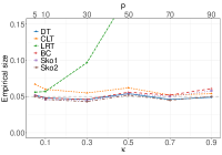
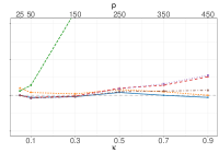
Figure 2: Empirical size of the directional test (DT), central limit theorem test (CLT), likelihood ratio test (LRT), Bartlett correction (BC) and two Skovgaard,’s modifications (Sko1 and Sko2) for hypothesis (8), at nominal level $\alpha=0.05$ given by the gray horizontal line. The left, middle and right panels correspond to $n_{i}=100,500,1000$, respectively ($g=3$).

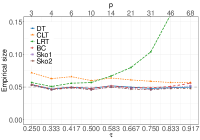
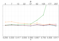
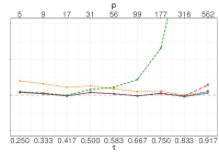
Figure S1: Empirical size of the directional test (DT), central limit theorem test (CLT), likelihood ratio test (LRT), Bartlett correction (BC) and two Skovgaard,’s modifications (Sko1 and Sko2) for hypothesis (8) in the paper, at nominal level $\alpha=0.05$ given by the gray horizontal line. The left, middle and right panels correspond to $n_{i}=100,500,1000$, respectively ($g=3$).

The empirical size, i.e. the actual probability of type I error, at nominal level $\alpha=0.05$ based on the null distribution of the various statistics is reported in Figure S1. The directional $p$-value performs very well across all different values of $p$, confirming the exactness result in Theorem 1, while the central limit theorem test is less accurate when $p$ is small. The test based on $W$ breaks down in all settings. Instead, the Bartlett correction $W_{BC}$ proves accurate for moderate values of $p$, as seen in He et al., (2021). However, the chi-square approximations for $W_{BC}$, $W^{*}$ and $W^{**}$ get unreliable as $p$ grows. Table 1 reports the empirical size in some extreme settings with $n_{i}\leq p\leq\sum_{i=1}^{g}n_{i}-g-1$. The results show that the chi-square approximations, $W$ $W_{BC}$, $W^{*}$ and $W^{**}$, can not work in such extreme setting, while the directional test is still feasible. The central limit theorem may break down with large $p$.

Table 1: Empirical size of the directional test (DT), central limit theorem test (CLT), likelihood ratio test (LRT), Bartlett correction (BC) and two Skovgaard,’s modifications (Sko1 and Sko2) for hypothesis (8) with $p=\kappa n_{i}$ and $n_{i}=100$, at nominal level $\alpha=0.05$.

$\kappa$ ($p$)	DT	CLT	LRT	BC	Sko1	Sko2
1.0 (100)	0.048	0.053	0.677	0.066	0.064	0.050
1.5 (150)	0.048	0.055	0.991	0.133	0.131	0.073
2.0 (200)	0.046	0.052	1.000	0.401	0.402	0.145
2.5 (250)	0.052	0.057	1.000	0.967	0.966	0.567
2.9 (290)	0.048	0.060	1.000	1.000	1.000	0.999

4.2 Heteroscedastic one-way MANOVA

The performance of the directional test for hypothesis (9) in the moderate dimensional multivariate normal framework is here evaluated via Monte Carlo simulations based on 10,000 replications. The directional test is again compared with the chi-square approximations for the likelihood ratio test and its modifications proposed by Skovgaard, (2001). When $g=2$, we also consider the $F$-approximation for the Behrens-Fisher test $T^{*2}$ by Nel and Merwe, (1986). The different testing approaches are evaluated in terms of empirical size. The result for $g=5,30$ are reported in Section S2.3 of the Supplemental material , and are in line with the ones available discussed below.

We generate the data matrix $y_{i}$ as $n_{i}$ independent replications from a multivariate normal distribution $N_{p}(\mu_{i},\Lambda_{i}^{-1}),i=1,\dots,g$. Under the null hypothesis $H_{\psi}$, we set $\mu_{i}=0_{p}$ and use an autoregressive structure for the covariance matrices, i.e. $\Lambda_{i}^{-1}=(\sigma_{jl})_{p\times p}=(\rho_{i}^{|j-l|})_{p\times p}$, with the $\rho_{i}$ chosen to an equally-spaced sequence from 0.1 to 0.9 of length $g$. In particular, when $g=2$, $\Lambda_{1}^{-1}=(0.1^{|j-l|})_{p\times p}$ and $\Lambda^{-1}_{2}=(0.9^{|j-l|})_{p\times p}$. We show results for $p=\lceil n_{i}\rceil^{\tau}$ with $\tau=j/24$, $j\in\{6,7,\dots,22\}$, $n_{i}\in\{100,500,1000\}$ and $g=2$. Note that for $n_{i}=1000$ the simulations results are based on $5000$ replications when $j\in\{21,22\}$ due to the expensive computational cost.

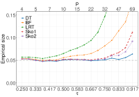
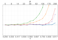
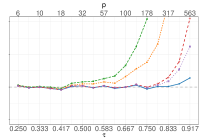
Figure 3: Empirical size of the directional test (DT), Behrens-Fisher test (BF) (Nel and Merwe,, 1986), likelihood ratio test (LRT), and two Skovgaard,’s modifications (Sko1 and Sko2) for hypothesis (9), at nominal level $\alpha=0.05$ given by the gray horizontal line. The left, middle and right panels correspond to $n_{i}=100,500,1000$, respectively ($g=3$).

Figure 3 reports the empirical size at the nominal level $\alpha=0.05$ under the null hypothesis for various statistics. The directional test is always more reliable than its competitors in terms of the empirical size, even if in this case it is not exact. Skovgaard,’s modifications are not as accurate when $p$ is large. Moreover, with $n_{i}$ increasing, the likelihood ratio test and the Behrens-Fisher test will not be valid and break down fast when $p=\lceil n_{i}\rceil^{\tau}$, even for moderate large values of $\tau$. Additional simulation results are showed in Table 2 for different structures of the covariance matrices: (I) identity matrix, $\Lambda_{i}^{-1}=I_{p}$; (II) compound symmetric matrix, $\Lambda^{-1}_{i}=(1-\rho_{i})I_{p}+\rho_{i}1_{p}1_{p}^{\top}$, with the same values of $\rho_{i}$ as in the autoregressive structure. Table 2 reports the empirical size at the nominal level $\alpha=0.05$ for $n_{i}=100$ and $p=\lceil n_{i}\rceil^{\tau}$, with covariance structures (I) and (II) and $g=2,30$. As expected, the likelihood ratio test performs in general very poorly, especially for larger values of $g$. Skovgaard,’s modifications are much more accurate but not as much as the directional test, whose excellent performance is confirmed. When $g=2$, the approximate solution for the Behrens-Fisher test seems reliable in the identity covariance matrix case, but not under compound symmetry.

Table 2: Empirical size of the directional test (DT), likelihood ratio test (LRT), two Skovgaard,’s modifications (Sko1 and Sko2), and Behrens-Fisher test (BF) (only for $g=2$) for hypothesis (9) at nominal level $\alpha=0.05$, with $n_{i}=100$ and $p=n_{i}^{\tau}$.

$\Lambda_{i}^{-1}$	$\tau$ ($p$)	$g=2$						$g=30$
		DT	BF	LRT	Sko1	Sko2		DT	LRT	Sko1	Sko2
(I)	10/24 (7)	0.051	0.051	0.058	0.051	0.051		0.048	0.118	0.049	0.048
	12/24 (10)	0.050	0.050	0.059	0.050	0.050		0.048	0.188	0.050	0.048
	14/24 (15)	0.050	0.050	0.069	0.050	0.050		0.048	0.382	0.051	0.048
	16/24 (22)	0.048	0.048	0.079	0.049	0.048		0.049	0.754	0.060	0.052
	18/24 (32)	0.053	0.052	0.110	0.054	0.053		0.050	0.993	0.087	0.061
	20/24 (47)	0.046	0.045	0.180	0.050	0.047		0.054	1.000	0.223	0.099
	22/24 (69)	0.054	0.052	0.377	0.066	0.059		0.048	1.000	0.928	0.404
(II)	10/24 (7)	0.050	0.054	0.059	0.050	0.050		0.049	0.118	0.049	0.048
	12/24 (10)	0.053	0.058	0.065	0.053	0.053		0.048	0.187	0.049	0.048
	14/24 (15)	0.048	0.062	0.076	0.050	0.049		0.049	0.383	0.052	0.050
	16/24 (22)	0.049	0.075	0.104	0.051	0.049		0.049	0.755	0.060	0.051
	18/24 (32)	0.050	0.104	0.171	0.057	0.054		0.050	0.993	0.085	0.059
	20/24 (47)	0.049	0.154	0.345	0.071	0.062		0.053	1.000	0.225	0.099
	22/24 (69)	0.081	0.296	0.766	0.174	0.136		0.048	1.000	0.932	0.408

4.3 Robustness to misspecification

In general, all the approaches examined so far rely on the assumed normal model and are not guaranteed to be robust under model misspecification. We can assess numerically the robustness of the various competitors using simulations. In this section, we consider three different distributions for the true generating process: multivariate $t$, multivariate skew-normal (Azzalini and Capitanio,, 1999) or multivariate Laplace. More in detail, a multivariate $t$ distribution with location $0_{p}$, scale matrix $I_{p}$ and degrees of freedom $5$, a multivariate skew-normal distribution with location $1_{p}$, scale matrix $\Omega=(\omega_{jl})=(0.2)^{|j-l|}$ and shape parameter $1_{p}$, and a multivariate Laplace distribution with mean vector $1_{p}$ and identity covariance matrix. Simulation results are based on $10,000$ replications.

For hypothesis (8), Figures S5–S6 show the empirical size at the nominal level $\alpha=0.05$ if the underling distribution is misspecified. We see that the directional test still maintains the hightest accuracy. For hypothesis (9), Figures 6–7 show the same relative pattern as that observed under the correct model specification in Figure 3. Hence, all solutions exhibit a similar behavior and seem robust to misspecification of the normal model, at least with respect to the three true data generating process we considered.

Figure 4: Empirical size for the directional test (DT), central limit theorem test (CLT), likelihood ratio test (LRT), Bartlett correction (BC) and two Skovgaard,’s modifications (Sko1 and Sko2) for hypothesis (8), at nominal level $\alpha=0.05$ given by the gray horizontal line. The left, middle and right panels correspond to multivariate $t$, multivariate skew-normal, and multivariate Laplace distributions of the true generating process, respectively, with $n_{i}=100$ and $g=3$.

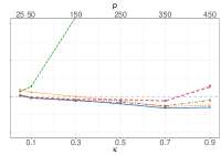
Figure 5: Empirical size for the directional test (DT), central limit theorem test (CLT), likelihood ratio test (LRT), Bartlett correction (BC) and two Skovgaard,’s modifications (Sko1 and Sko2, respectively) for hypothesis (8), at nominal level $\alpha=0.05$ given by the gray horizontal line. The left, middle and right panels correspond to multivariate $t$, multivariate skew-normal, and multivariate Laplace distributions of the true generating process, respectively, with $n_{i}=500$ and $g=3$.

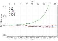
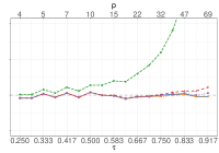
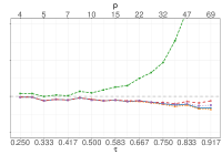
Figure 6: Empirical size for the directional test (DT), Behrens-Fisher test (BF), likelihood ratio test (LRT), and two Skovgaard,’s modifications (Sko1 and Sko2) for hypothesis (9), at nominal level $\alpha=0.05$ given by the gray horizontal line. The left, middle and right panels correspond to multivariate $t$, multivariate skew-normal, and multivariate Laplace distributions if the true generating process, respectively, with $n_{i}=100$ and $g=2$.

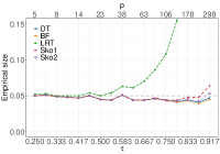
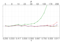
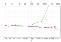
Figure 7: Empirical size for the directional test (DT), Behrens-Fisher test (BF), likelihood ratio test (LRT), and two Skovgaard,’s modifications (Sko1 and Sko2) for hypothesis (9), at nominal level $\alpha=0.05$ given by the gray horizontal line. The left, middle and right panels correspond to multivariate $t$, multivariate skew-normal, and multivariate Laplace distributions of the true generating process, respectively, with $n_{i}=500$ and $g=2$.

5 Conclusions and discussion

In this paper, we have developed the directional test for one-way MANOVA problems when the data dimension is comparable with the sample size. The directional $p$-value has been proved exactly uniformly distributed, provided that $\sum_{i=1}^{k}n_{i}\geq p+g+1$, when testing the equality of normal mean vectors with identical covariance matrix. Such a finding is supported by the numerical studies. Moreover, simulations in moderate dimensional scenarios in the heteroscedastic one-way MANOVA framework indicate that the directional test outperforms its competitors in terms of empirical null distribution even in the more general setting with different covariance matrices. Formal conditions for the validity of the various methods in this scenario could be developed using recent results on the accuracy of the saddlepoint approximation in moderate dimensional regimes (Tang and Reid,, 2021). Further investigations have showed that all the likelihood-based solutions examined are robust to the misspecification of the assumed multivariate normal model.

Supplementary Material

Supplementary material includes some additional simulation studies.

Appendix A

A.1 Correction factor $\gamma$ in Skovgaard,’s modifications

The general expression for $\gamma$ appearing in Skovgaard,’s modified versions of W (3) can be written as

$$\gamma=\frac{\left\{(s-s_{\psi})^{\top}J_{\varphi\varphi}(\hat{\varphi}_{\psi})^{-1}(s-s_{\psi})\right\}^{d/2}}{W^{d/2-1}(\hat{\varphi}-\hat{\varphi}_{\psi})^{\top}(s-s_{\psi})}\left\{\frac{|{J}_{\varphi\varphi}(\hat{\varphi}_{\psi})|}{|{J}_{\varphi\varphi}(\hat{\varphi})|}\right\}^{1/2}\left\{\frac{|{J}_{\lambda\lambda}(\hat{\varphi}_{\psi})|}{|{I}_{\lambda\lambda}(\hat{\varphi}_{\psi})|}\right\}^{1/2},$$ (A1)

where $J_{\lambda\lambda}$ and $I_{\lambda\lambda}$ are the observed and expected information matrices, respectively, refered to the nuisance parameter $\lambda$. For calculating the $p$-value, the quantity (A1) is evaluated at $s=s^{0}=0_{q}$, corresponding to the observed data point $y^{0}$. In particular, if $\lambda$ is a component or a linear function of the canonical parameter, as in Section 3.1, the last factor in (A1) equals 1.

A.2 Observed information matrix

When testing hypothesis (8), the saddlepoint approximation (Pace and Salvan,, 1997, Section 10) and the correction factor $\gamma$ in (3) require the computation of the observed information matrix $J_{\varphi\varphi}(\varphi)$. This has the block form

$$J_{\varphi\varphi}(\varphi) =\left(\begin{array}[]{cc}J_{\xi\xi}&J_{\xi\text{vech}(\Lambda)}\\ J_{\text{vech}(\Lambda)\xi}&J_{\text{vech}(\Lambda)\text{vech}(\Lambda)}\end{array}\right),$$ (A4)

$$\text{with}\;J_{\xi\xi}=\left(\begin{array}[]{cccc}n_{1}\Lambda^{-1}&0_{p\times p}&\cdot&0_{p\times p}\\ 0_{p\times p}&n_{2}\Lambda^{-1}&\cdot&0_{p\times p}\\ \vdots&\vdots&\vdots&\vdots\\ 0_{p\times p}&0_{p\times p}&\cdot&n_{g}\Lambda^{-1}\end{array}\right),\;J_{\text{vech}(\Lambda)\xi}^{\top}=J_{\xi\text{vech}(\Lambda)}=\left(\begin{array}[]{c}-n_{1}(\xi_{1}^{\top}\Lambda^{-1}\otimes\Lambda^{-1})D_{p}\\ -n_{2}(\xi_{2}^{\top}\Lambda^{-1}\otimes\Lambda^{-1})D_{p}\\ \vdots\\ -n_{k}(\xi_{g}^{\top}\Lambda^{-1}\otimes\Lambda^{-1})D_{p}\end{array}\right)$$ (A13)

and $J_{\text{vech}(\Lambda)\text{vech}(\Lambda)}=\sum_{i=1}^{g}\frac{n_{i}}{2}D_{p}^{\top}\Lambda^{-1}(I_{p}+2\xi_{i}\xi_{i}^{\top}\Lambda^{-1})\otimes\Lambda^{-1}D_{p},$ where $\otimes$ denotes the Kronecker product (see, for instance, Lauritzen,, 1996). Then, the determinant of $J_{\varphi\varphi}(\varphi)$ can be computed as

$$|J_{\varphi\varphi}(\varphi)|=|J_{\xi\xi}||C_{2}|,$$

where $C_{2}=J_{\text{vech}(\Lambda)\text{vech}(\Lambda)}-J_{\text{vech}(\Lambda)\xi}J_{\xi\xi}^{-1}J_{\xi\text{vech}(\Lambda)}=\sum_{i=1}^{g}\frac{n_{i}}{2}D_{p}^{\top}\Lambda^{-1}(I_{p}+2\xi_{i}\xi_{i}^{\top}\Lambda^{-1})\otimes\Lambda^{-1}D_{p}-\sum_{i=1}^{g}n_{i}D_{p}^{\top}\Lambda^{-1}$ $\xi_{i}\xi_{i}^{\top}$ $\Lambda^{-1}\otimes\Lambda^{-1}D_{p}$ $=\frac{n}{2}D_{p}^{\top}\left(\Lambda^{-1}\otimes\Lambda^{-1}\right)D_{p}$.

After some algebra, we get

$$|J_{\varphi\varphi}(\varphi)|=\left(\prod_{i=1}^{g}n_{i}^{p}\right)|\Lambda^{-1}|^{g}n^{\frac{p(p+1)}{2}}2^{-p}|\Lambda^{-1}|^{p+1}\propto|\Lambda^{-1}|^{p+g+1}.$$

Appendix Appendix B

B.1 Proof of Lemma 1

Recall that $\hat{\Lambda}^{-1}(t)=\hat{\Lambda}_{0}^{-1}-t^{2}A/n=\hat{\Lambda}^{-1}+(1-t^{2})A/n$ with $\hat{\Lambda}_{0}^{-1}=\hat{\Lambda}^{-1}+A/n$, where $A=\sum_{i=1}^{g}n_{i}(\bar{y}_{i}-\bar{y})(\bar{y}_{i}-\bar{y})^{\top}$. If $t\in[0,1]$ the result is straightforward, since, for all $x\in\mathbb{R}^{p}$, $x^{\top}\hat{\Lambda}^{-1}(t)x=x^{\top}\hat{\Lambda}^{-1}x/n+(1-t^{2})x^{\top}Ax/n>0$. Let us focus on the case $t>1$. We rewrite the estimator $\hat{\Lambda}^{-1}(t)$ as

$$\hat{\Lambda}^{-1}(t)=B_{0}^{\top}\left\{I_{p}-t^{2}(B_{0}^{\top})^{-1}(A/n)B_{0}^{-1}\right\}B_{0},$$

with the square root $B_{0}$ of $\hat{\Lambda}_{0}^{-1}$ such that $\hat{\Lambda}_{0}^{-1}=B_{0}^{\top}B_{0}$. According to the eigen decomposition, the matrix $(B_{0}^{\top})^{-1}(A/n)B_{0}^{-1}=PQP^{\top}$ with an orthogonal matrix $P$ whose columns are eigenvectors of $(B_{0}^{\top})^{-1}(A/n)B_{0}^{-1}$ and a diagonal matrix $Q$ whose diagonal elements are the eigenvalues of $(B_{0}^{\top})^{-1}(A/n)B_{0}^{-1}$. Then, we have $\hat{\Lambda}^{-1}(t)=B_{0}^{\top}P\{I_{p}-t^{2}Q\}P^{\top}B_{0}$. Therefore, checking that $\hat{\Lambda}^{-1}(t)$ is positive definite is equivalent to checking that $I_{p}-t^{2}Q$ is positive definite. Indeed, for all $x\in\mathbb{R}^{p},x\neq 0$, then

$$x^{\top}\hat{\Lambda}^{-1}x = x^{\top}B^{\top}_{0}P\{I_{p}-t^{2}Q\}P^{\top}B_{0}x$$

$$= \tilde{x}^{\top}\{I_{p}-t^{2}Q\}\tilde{x}>0,$$

where $\tilde{x}=P^{\top}B_{0}x$, with $\tilde{x}\neq 0$ if $x\neq 0$.

Next, the positive definition of $I_{p}-t^{2}Q$ should be proved. It is equivalent to checking that all elements of the diagonal matrix $I_{p}-t^{2}Q=\text{diag}(1-t^{2}\nu_{l})$ are positive, where $\nu_{l},l\in\{1,\dots,p\}$, are the eigenvalues of the matrix $(B_{0}^{\top})^{-1}(A/n)B_{0}^{-1}$. We now need to find out the largest $t$ such that $1-t^{2}\nu_{l}>0$, $l\in\{1,\dots,p\}$. It is easy to get the largest value of $t$ for which $\hat{\Lambda}^{-1}(t)$ is positive definite equals $t_{\text{sup}}=\sqrt{1/\nu_{(p)}}$, where $\nu_{p}$ is the maximum eigenvalue of the matrix $(B_{0}^{-1})^{\top}AB_{0}^{-1}/n$.

Therefore, $\hat{\Lambda}^{-1}(t)$ is positive definite in $t\in[0,\sqrt{1/\nu_{(p)}}]$.

B.2 Proof of Theorem 1

Suppose $y_{i}=[y_{i1}\cdots y_{in_{i}}]^{\top}$, with $y_{ij}\sim N_{p}(\mu_{i},\Lambda^{-1})$, $i=1,\dots,g$ and $j=1,\dots,n_{i}$. The log-likelihood for the canonical parameter $\varphi$ is

$$\ell(\varphi;s)=\sum_{i=1}^{g}-\frac{n_{i}}{2}\log|\Lambda^{-1}|-\frac{1}{2}{\text{tr}}(\Lambda B_{i})-\frac{n_{i}}{2}(\bar{y}_{i}-\mu_{i})^{\top}\Lambda(\bar{y}_{i}-\mu_{i}),$$ (B1)

where $B_{i}=y_{i}^{\top}y_{i}-n_{i}\bar{y}_{i}\bar{y}_{i}^{\top}$. The maximum likelihood estimate and the constrained maximum likelihood estimate are respectively $\hat{\varphi}=\{\hat{\xi}^{\top}_{1},\ldots,\hat{\xi}^{\top}_{k},\text{vech}(\hat{\Lambda})^{\top}\}^{\top}$ $=\{\bar{y}_{1}^{\top}\hat{\Lambda},\ldots,\bar{y}_{g}^{\top}\hat{\Lambda},\text{vech}(\hat{\Lambda})^{\top}\}^{\top}$ and $\hat{\varphi}_{\psi}=\{\bar{y}^{\top}{\hat{\Lambda}_{0}},\ldots,\bar{y}^{\top}{\hat{\Lambda}_{0}},$ $\text{vech}({\hat{\Lambda}_{0}})^{\top}\}^{\top}$. Evaluating (B1) at the unconstrained and constrained maximum likelihood estimates for $\varphi$, we have $\ell(\hat{\varphi};s)=-n/2\log|\hat{\Lambda}^{-1}|-{np}/2$ and $\ell(\hat{\varphi}_{\psi};s)=2^{-1}\sum_{i=1}^{g}-{n_{i}}$ $\log|{\hat{\Lambda}_{0}}^{-1}|-{n_{i}}p$, respectively. Then, under the null hypothesis $H_{\psi}$, using the fact that $|J_{\varphi\varphi}(\hat{\varphi})|\propto|\hat{\Lambda}^{-1}|^{p+g+1}$, the saddlepoint approximation (5) is

$$h(s;\psi) = \left[\prod_{i=1}^{g}c_{i1}|\hat{\Lambda}_{0}^{-1}|^{-\frac{1}{2}}\exp\left\{-\frac{n_{i}}{2}(\bar{y}_{i}-\hat{\mu}_{\psi})^{\top}\hat{\Lambda}_{0}(\bar{y}_{i}-\hat{\mu}_{\psi})\right\}\right]$$ (B2)

$$\;\;\times c_{2}|\hat{\Lambda}_{0}^{-1}|^{\frac{n-1}{2}}\exp\left\{-\frac{n}{2}{\text{tr}}(\hat{\Lambda}_{0}\hat{\Lambda}^{-1})\right\}|\hat{\Lambda}^{-1}|^{\frac{n-p-g-1}{2}}.$$

Expression (B2) equals the exact joint distribution of $\bar{y}_{1},\dots,\bar{y}_{g}$ and $\hat{\Lambda}^{-1}$ if $c_{i1}=(2\pi)^{-p/2}$ and $c_{2}=\left(\frac{n}{2}\right)^{p(n-1)/2}\Gamma_{p}\left(\frac{n-g}{2}\right)^{-1}$ and with fixed values of $\hat{\mu}_{\psi}$ and $\hat{\Lambda}_{0}^{-1}$. Indeed, the constrained maximum likelihood estimates are fixed and equal to their observed values when we consider the saddlepoint approximation along the line $s(t)$ under $H_{\psi}$. Moreover, we have the unconstrained maximum likelihood estimates $\hat{\mu}(t)=t\bar{y}_{i}+(1-t)\bar{y}$ and $\hat{\Lambda}^{-1}(t)=\hat{\Lambda}_{0}^{-1}-t^{2}A/n$. Then, the saddlepoint approximation to the conditional distribution of $s(t)$ under $H_{\psi}$ follows from (B2) and is equal to

$$h\{s(t);\psi\} = \prod_{i=1}^{g}c_{i1}|\hat{\Lambda}_{0}^{-1}|^{-\frac{1}{2}}\exp\left[-\frac{n_{i}}{2}\{\hat{\mu}_{i}(t)-\hat{\mu}_{\psi}\}^{\top}\hat{\Lambda}_{0}\{\hat{\mu}_{i}(t)-\hat{\mu}_{\psi}\}\right]$$

$$\;\;\times c_{2}|\hat{\Lambda}_{0}^{-1}|^{\frac{n-1}{2}}\exp\left[-\frac{n}{2}{\text{tr}}\{\hat{\Lambda}_{0}\hat{\Lambda}(t)^{-1}\}\right]|\hat{\Lambda}(t)^{-1}|^{\frac{n-p-g-1}{2}}$$

$$\propto \prod_{i=1}^{g}\exp\left[-\frac{n_{i}}{2}\{t\bar{y}_{i}+(1-t)\bar{y}-\bar{y}\}^{\top}\hat{\Lambda}_{0}\{t\bar{y}_{i}+(1-t)\bar{y}-\bar{y}\}\right]$$

$$\;\;\times\exp\left[-\frac{n}{2}{\text{tr}}\{\hat{\Lambda}_{0}(\hat{\Lambda}_{0}^{-1}-t^{2}A/n)\}\right]|\hat{\Lambda}^{-1}(t)|^{\frac{n-p-g-1}{2}}$$

$$\propto \exp\left\{-\frac{1}{2}t^{2}\sum_{i=1}^{g}(\bar{y}_{i}-\bar{y})^{\top}\hat{\Lambda}_{0}(\bar{y}_{i}-\bar{y})\right\}\exp\left\{\frac{1}{2}t^{2}{\text{tr}}(\hat{\Lambda}_{0}A)\right\}|\hat{\Lambda}^{-1}(t)|^{\frac{n-p-g-1}{2}}$$

$$\propto |\hat{\Lambda}^{-1}(t)|^{\frac{n-p-g-1}{2}}.$$

Since the saddlepoint approximation $h\{s(t);\psi\}$ is in fact exact, up to a normalizing constant, the integral in the denominator of the directional $p$-value (7) is the normalizing constant of the conditional distribution of $||s||$ given the direction $s^{0}/||s^{0}||$. The directional $p$-value is then the exact probability of $||s||>||s^{0}||$ given the direction $s^{0}/||s^{0}||$ under the null hypothesis $H_{\psi}$, and hence is exactly uniformly distributed.

B.3 Proof of Proposition 1

First, we express the estimate $\hat{\Lambda}^{-1}(t)=\hat{\Lambda}_{0}^{-1}-t^{2}A/n$, where $n=n_{1}+n_{2}$, as

$$\hat{\Lambda}^{-1}(t)= \hat{\Lambda}_{0}^{-1}-t^{2}\sum_{i=1}^{2}n_{i}(\bar{y}_{i}-\bar{y})(\bar{y}_{i}-\bar{y})^{\top}/n,$$

where $\bar{y}=(n_{1}\bar{y}_{1}+n_{2}\bar{y}_{2})/n$. Moreover, we have

$$\sum_{i=1}^{2}n_{i}(\bar{y}_{i}-\bar{y})(\bar{y}_{i}-\bar{y})^{\top}= \;n_{1}(\bar{y}_{1}-\bar{y})(\bar{y}_{1}-\bar{y})^{\top}+n_{2}(\bar{y}_{2}-\bar{y})(\bar{y}_{2}-\bar{y})^{\top}$$

$$= \;\frac{n_{1}n_{2}(\bar{y}_{1}-\bar{y}_{2})(\bar{y}_{1}-\bar{y}_{2})^{\top}}{n},$$

since

$$n_{1}\bar{y}_{1}\bar{y}_{1}^{\top}+n_{2}\bar{y}_{2}\bar{y}_{2}^{\top}= \frac{n_{1}^{2}\bar{y}_{1}\bar{y}_{1}^{\top}+n_{1}n_{2}\bar{y}_{1}\bar{y}_{1}^{\top}+n_{1}n_{2}\bar{y}_{2}\bar{y}_{2}^{\top}+n_{2}^{2}\bar{y}_{2}\bar{y}_{2}^{\top}}{n},$$

$$n\bar{y}\bar{y}^{\top}= \frac{n_{1}^{2}\bar{y}_{1}\bar{y}_{1}^{\top}+n_{1}n_{2}\bar{y}_{1}\bar{y}_{2}^{\top}+n_{1}n_{2}\bar{y}_{2}\bar{y}_{1}^{\top}+n_{2}^{2}\bar{y}_{2}\bar{y}_{2}^{\top}}{n}.$$

Then

$$\hat{\Lambda}^{-1}(t)= \hat{\Lambda}_{0}^{-1}-t^{2}\frac{n_{1}n_{2}}{n^{2}}(\bar{y}_{1}-\bar{y}_{2})(\bar{y}_{1}-\bar{y}_{2})^{\top},$$

$$|\hat{\Lambda}^{-1}(t)|= |\hat{\Lambda}_{0}^{-1}|\left\{1-t^{2}\frac{n_{1}n_{2}}{n^{2}}(\bar{y}_{1}-\bar{y}_{2})^{\top}\hat{\Lambda}_{0}(\bar{y}_{1}-\bar{y}_{2})\right\}.$$

The integrand function in the directional $p$-value (7) along the line $s(t)$ can then be simplified to

$$g(t)=t^{d-1}|\hat{\Lambda}^{-1}(t)|^{\frac{n-p-3}{2}}\propto t^{d-1}\left\{1-t^{2}\frac{n_{1}n_{2}}{n^{2}}(\bar{y}_{1}-\bar{y}_{2})^{\top}\hat{\Lambda}_{0}(\bar{y}_{1}-\bar{y}_{2})\right\}^{\frac{n-p-3}{2}},$$

thus the directional $p$-value under the null hypothesis $H_{\psi}$ takes the form

$$p(\psi)=\frac{\int_{1}^{t_{\text{sup}}}t^{d-1}\left\{1-t^{2}\frac{n_{1}n_{2}}{n^{2}}(\bar{y}_{1}-\bar{y}_{2})^{\top}\hat{\Lambda}_{0}(\bar{y}_{1}-\bar{y}_{2})\right\}^{\frac{n-p-3}{2}}\text{d}t}{\int_{0}^{t_{\text{sup}}}t^{d-1}\left\{1-t^{2}\frac{n_{1}n_{2}}{n^{2}}(\bar{y}_{1}-\bar{y}_{2})^{\top}\hat{\Lambda}_{0}(\bar{y}_{1}-\bar{y}_{2})\right\}^{\frac{n-p-3}{2}}\text{d}t},$$

where $t_{\text{sup}}=\left\{\frac{n_{1}n_{2}}{n^{2}}(\bar{y}_{1}-\bar{y}_{2})^{\top}\hat{\Lambda}_{0}(\bar{y}_{1}-\bar{y}_{2})\right\}^{-1/2}$. In order to make the notation more compact, we define $C=\frac{n_{1}n_{2}}{n^{2}}(\bar{y}_{1}-\bar{y}_{2})^{\top}\hat{\Lambda}_{0}(\bar{y}_{1}-\bar{y}_{2})$, so that $t_{\text{sup}}=C^{-1/2}$. We can now rewrite the directional $p$-value as

$$p(\psi)=\frac{\int_{1}^{C^{-1/2}}t^{d-1}\left\{1-t^{2}C\right\}^{\frac{n-p-3}{2}}\text{d}t}{\int_{0}^{C^{-1/2}}t^{d-1}\left\{1-t^{2}C\right\}^{\frac{n-p-3}{2}}\text{d}t}.$$ (B3)

Since the Hotelling’s $T^{2}$ statistic has Hotelling’s $T^{2}$ distribution, i.e., $T^{2}\sim T^{2}(p,n-p-1)$ with degrees of freedom $df_{1}=p$ and $df_{2}=n-p-1$, we change variable from $t$ to $\left\{C\left(\frac{df_{2}}{df_{1}}x+1\right)\right\}^{-1/2}$.

The following steps are used to compute the numerator in the directional $p$-value (B3).

Step 1. Change of the integration interval:

$$1\leq t\leq C^{-1/2}\Leftrightarrow 1\leq\left\{C\left(\frac{df_{2}}{df_{1}}x+1\right)\right\}^{-1/2}\leq C^{-1/2}$$

$$\Leftrightarrow C\leq\left(\frac{df_{2}}{df_{1}}x+1\right)^{-1}\leq 1\Leftrightarrow 1\leq\frac{df_{2}}{df_{1}}x+1\leq C^{-1}$$

$$\Leftrightarrow 0\leq\frac{df_{2}}{df_{1}}x\leq C^{-1}-1\Leftrightarrow 0\leq x\leq\frac{df_{1}}{df_{2}}\frac{1-C}{C}$$

hence the new integral is on $\left[0,\frac{df_{1}}{df_{2}}\frac{1-C}{C}\right]$.

Step 2. Change of variable from $t$ to $x$:

$$\int_{1}^{C^{-1/2}}t^{d-1}\left\{1-t^{2}C\right\}^{\frac{n-p-3}{2}}\text{d}t$$

$$= \int_{0}^{\frac{df_{1}}{df_{2}}\frac{1-C}{C}}\left\{C\left(\frac{df_{2}}{df_{1}}x+1\right)\right\}^{-\frac{d-1}{2}}\left\{1-C^{-1}\left(\frac{df_{2}}{df_{1}}x+1\right)^{-1}C\right\}^{\frac{n-p-3}{2}}\text{d}\left\{C\left(\frac{df_{2}}{df_{1}}x+1\right)\right\}^{-\frac{1}{2}},$$

where $d=p(k-1)=p$. Then we get

$${\text{d}\left\{C\left(\frac{df_{2}}{df_{1}}x+1\right)\right\}^{-\frac{1}{2}}}=C^{-1/2}(-\frac{1}{2})\left(\frac{df_{2}}{df_{1}}x+1\right)^{-\frac{3}{2}}\frac{df_{2}}{df_{1}}{\text{d}x},$$

and

$$\int_{1}^{C^{-1/2}}t^{d-1}\left\{1-t^{2}C\right\}^{\frac{n-p-3}{2}}\text{d}t$$

$$= c\int_{0}^{\frac{df_{1}}{df_{2}}\frac{1-C}{C}}\left(\frac{df_{2}}{df_{1}}x+1\right)^{-\frac{p-1}{2}}\left\{1-\left(\frac{df_{2}}{df_{1}}x+1\right)^{-1}\right\}^{\frac{n-p-3}{2}}\left(\frac{df_{2}}{df_{1}}x+1\right)^{-\frac{3}{2}}\text{d}x$$

$$= c\int_{0}^{\frac{df_{1}}{df_{2}}\frac{1-C}{C}}\left(\frac{df_{2}}{df_{1}}x+1\right)^{-\frac{p-1+3}{2}}\left\{\frac{\frac{df_{2}}{df_{1}}x+1-1}{\frac{df_{2}}{df_{1}}x+1}\right\}^{\frac{n-p-3}{2}}\text{d}x$$

$$= c\int_{0}^{\frac{df_{1}}{df_{2}}\frac{1-C}{C}}\left(\frac{df_{2}}{df_{1}}x+1\right)^{-\frac{n-p-1+p}{2}}\left(\frac{df_{2}}{df_{1}}x\right)^{\frac{n-p-1}{2}-1}\text{d}x$$

$$= c\int_{0}^{\frac{df_{1}}{df_{2}}\frac{1-C}{C}}\left(\frac{df_{2}}{df_{1}}x+1\right)^{-\frac{df_{2}+df_{1}}{2}}\left(\frac{df_{2}}{df_{1}}x\right)^{\frac{df_{2}}{2}-1}\text{d}x$$

$$= c^{\prime}F\left(\frac{df_{1}}{df_{2}}\frac{1-C}{C},df_{2},df_{1}\right),$$

where $F(X,df_{2},df_{1})$ is the cumulative distribution function of a random variable $X$ following a $F$-distribution with degrees of freedom $df_{2}$ and $df_{1}$. Since if $X\sim F(df_{2},df_{1})$, then $X^{-1}\sim F(df_{1},df_{2})$, we can express the directional $p$-value as

$$p(\psi)=1-F\left(\frac{df_{2}}{df_{1}}\frac{C}{1-C},df_{1},df_{2}\right).$$

According to the Sherman-Morrison formula (see also McCormack et al.,, 2019, Section 4.2), we have that $C=\frac{\left.{n_{1}n_{2}}(\bar{y}_{1}-\bar{y}_{2})^{\top}\hat{\Lambda}(\bar{y}_{1}-\bar{y}_{2})\right/{n}}{1+\left.{n_{1}n_{2}}(\bar{y}_{1}-\bar{y}_{2})^{\top}\hat{\Lambda}(\bar{y}_{1}-\bar{y}_{2})\right/{n}}$ and

$$\frac{df_{2}}{df_{1}}\frac{C}{1-C}= \frac{n-p-1}{p}\cdot\frac{n_{1}n_{2}}{n^{2}}(\bar{y}_{1}-\bar{y}_{2})^{\top}\hat{\Lambda}(\bar{y}_{1}-\bar{y}_{2})$$

$$= \frac{n-p-1}{p}\cdot\frac{T^{2}}{n_{1}+n_{2}-2},$$

with $T^{2}=\left.{n_{1}n_{2}}(\bar{y}_{1}-\bar{y}_{2})^{\top}S^{-1}(\bar{y}_{1}-\bar{y}_{2})\right/{n}$ and $S=\left.{n}\hat{\Lambda}^{-1}\right/{(n_{1}-n_{2}-2)}$. Since $\left.{(n-p-1)}{T^{2}}\right/\{p(n_{1}+n_{2}-2)\}\sim F(p,n-p-1)$, the directional test is identical to the Hotelling $T^{2}$ test.

Supplementary material to Directional testing for one-way MANOVA in divergent dimensions

Appendix S1 Simulation studies for Homoscedastic one-way MANOVA

This section reports additional empirical result for homoscedastic one-way MANOVA in the multivariate normal framework. We compare the performance of exact directional test (DT) with other five approximate approaches: the central limite theorem test (CLT), log-likelihood ratio test (LRT), Bartlett correction (BC) and two Skovgaard,’s modifications (Sko1 and Sko2). The six tests are evaluated in terms of empirical size. The simulation results are computed via Monte Carlo simulation based on 10,000 replications.

S1.1 Empirical results for moderate setup

Groups of size $n_{i},i\in\{1,\dots,g\}$, are generated from a $p$-variate standard normal distribution $N_{p}(0_{p},I_{p})$ under the null hypothesis. For each simulation experiment, we show results for $p=\lfloor n_{i}^{\tau}\rfloor$ with $\tau=j/24$, $j\in\{6,8,\cdots,22\}$ and $n_{i}\in\{100,500,1000\}$. Throughout, we set $g=3$ and $n_{1}=n_{2}=n_{3}$.

Table S1: Empirical size of the directional test (DT), central limit theorem test (CLT), likelihood ratio test (LRT), Bartlett correction (BC) and two Skovgaard,’s modifications (Sko1 and Sko2) for hypothesis (8) in the paper with $n_{i}=100,500,1000$, at nominal level $\alpha=0.05$.

$n_{i}$	$\tau(p)$	DT	CLT	LRT	BC	Sko1	Sko2
100	0.250 (3)	0.054	0.072	0.057	0.054	0.053	0.053
	0.333 (4)	0.047	0.063	0.051	0.047	0.046	0.046
	0.417 (6)	0.050	0.066	0.056	0.050	0.049	0.049
	0.500 (10)	0.048	0.060	0.057	0.048	0.046	0.046
	0.580 (14)	0.052	0.064	0.067	0.052	0.050	0.050
	0.667 (21)	0.050	0.061	0.080	0.049	0.048	0.047
	0.750 (31)	0.048	0.059	0.104	0.049	0.046	0.046
	0.833 (46)	0.049	0.057	0.161	0.051	0.049	0.048
	0.917 (68)	0.050	0.057	0.311	0.056	0.052	0.048
500	0.250 (4)	0.051	0.068	0.052	0.051	0.051	0.051
	0.333 (7)	0.053	0.070	0.055	0.053	0.053	0.053
	0.417 (13)	0.051	0.063	0.054	0.051	0.051	0.051
	0.500 (22)	0.050	0.061	0.056	0.050	0.050	0.050
	0.580 (37)	0.048	0.056	0.058	0.048	0.048	0.048
	0.667 (62)	0.055	0.063	0.078	0.055	0.054	0.054
	0.750 (105)	0.050	0.054	0.105	0.051	0.050	0.049
	0.833 (177)	0.054	0.058	0.222	0.056	0.055	0.054
	0.917 (297)	0.047	0.050	0.609	0.057	0.056	0.049
1000	0.250 (5)	0.054	0.070	0.055	0.054	0.054	0.054
	0.333 (9)	0.052	0.066	0.053	0.053	0.052	0.052
	0.417 (17)	0.049	0.061	0.050	0.049	0.049	0.049
	0.500 (31)	0.054	0.063	0.058	0.054	0.054	0.054
	0.580 (56)	0.052	0.059	0.061	0.052	0.052	0.052
	0.667 (99)	0.049	0.055	0.072	0.049	0.049	0.049
	0.750 (177)	0.053	0.056	0.116	0.053	0.053	0.052
	0.833 (316)	0.048	0.050	0.261	0.049	0.049	0.048
	0.917 (562)	0.053	0.055	0.794	0.064	0.065	0.056

S1.2 Empirical results for large number $k$ of groups

Table S2: Empirical size of the directional test (DT), central limit theorem test (CLT), likelihood ratio test (LRT), Bartlett correction (BC) and two Skovgaard,’s modifications (Sko1 and Sko2) for hypothesis (8) in the paper with $p=n_{i}^{\tau}$, $n_{i}=100$ and $g=30$, at nominal level $\alpha=0.05$

$\tau(p)$	DT	CLT	LRT	BC	Sko1	Sko2
0.250 (3)	0.053	0.060	0.057	0.053	0.053	0.053
0.333 (4)	0.050	0.057	0.055	0.050	0.050	0.050
0.417 (6)	0.050	0.056	0.057	0.050	0.050	0.050
0.500 (10)	0.049	0.053	0.059	0.049	0.049	0.049
0.580 (14)	0.051	0.056	0.064	0.052	0.051	0.051
0.667 (21)	0.050	0.054	0.071	0.050	0.050	0.050
0.750 (31)	0.052	0.054	0.080	0.052	0.052	0.052
0.833 (46)	0.048	0.051	0.095	0.049	0.048	0.048
0.917 (68)	0.054	0.056	0.137	0.054	0.054	0.053

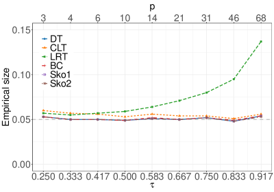
Figure S2: Empirical size of the directional test (DT), central limit theorem test (CLT), likelihood ratio test (LRT), Bartlett correction (BC) and two Skovgaard,’s modifications (Sko1 and Sko2) for hypothesis (8) in the paper with $n_{i}=100$ and $g=30$, at nominal level $\alpha=0.05$ given by the gray horizontal line.

S1.3 Empirical results for the setup of He et al., (2021, Section A.3)

In each Monte Carlo experiment, we show results for $p=\lfloor n^{\tau}\rfloor$ with $n=\sum_{i=1}^{g}n_{i}$. Under the null hypothesis, we set $g=3$, $n_{1}=n_{2}=n_{3}$, $\tau=j/24$ with $j\in\{6,8,\cdots,22\}$ and $n_{i}=100$.

Table S3: Empirical size of the directional test (DT), central limit theorem test (CLT), likelihood ratio test (LRT), Bartlett correction (BC) and two Skovgaard,’s modifications (Sko1 and Sko2) for hypothesis (8) in the paper with $p=n^{\tau}$ and $n=\sum_{i=1}^{3}100=300$, at nominal level $\alpha=0.05$.

$\tau$ ($p$)	DT	CLT	LRT	BC	Sko1	Sko2
0.250 (4)	0.048	0.064	0.052	0.047	0.046	0.046
0.333 (6)	0.049	0.066	0.056	0.049	0.047	0.047
0.417 (10)	0.050	0.064	0.061	0.050	0.049	0.049
0.500 (17)	0.053	0.065	0.074	0.053	0.051	0.051
0.583 (27)	0.046	0.056	0.088	0.047	0.045	0.045
0.667 (44)	0.051	0.060	0.157	0.053	0.050	0.049
0.750 (72)	0.048	0.054	0.347	0.054	0.052	0.047
0.833 (115)	0.050	0.056	0.832	0.078	0.077	0.057
0.917 (186)	0.044	0.049	1.000	0.280	0.278	0.106

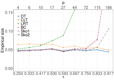
Figure S3: Empirical size of the directional test (DT), central limit theorem test (CLT), likelihood ratio test (LRT), Bartlett correction (BC) and two Skovgaard,’s modifications (Sko1 and Sko2) for hypothesis (8) in the paper with $p=n^{\tau}$ and $n=\sum_{i=1}^{3}100=300$, at nominal level $\alpha=0.05$ given by the gray horizontal line.

Table S4: Empirical size of the directional test (DT), central limit theorem test (CLT), likelihood ratio test (LRT), Bartlett correction (BC) and two Skovgaard,’s modifications (Sko1 and Sko2) for hypothesis (8) in the paper with $p=n^{\tau}$ and $n=\sum_{i=1}^{3}500=1500$, at nominal level $\alpha=0.05$.

$\tau$ ($p$)	DT	CLT	LRT	BC	Sko1	Sko2
0.250 (6)	0.052	0.068	0.053	0.052	0.052	0.052
0.333 (11)	0.051	0.063	0.053	0.051	0.050	0.050
0.417 (21)	0.050	0.059	0.053	0.050	0.049	0.049
0.500 (38)	0.051	0.060	0.062	0.051	0.051	0.051
0.583 (71)	0.051	0.059	0.080	0.051	0.050	0.050
0.667 (131)	0.051	0.056	0.146	0.052	0.051	0.051
0.750 (241)	0.052	0.057	0.402	0.058	0.058	0.053
0.833 (443)	0.052	0.056	0.976	0.081	0.083	0.063
0.917 (815)	0.049	0.051	1.000	0.420	0.462	0.171

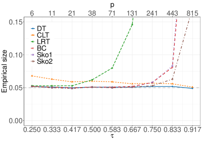
Figure S4: Empirical size of the directional test (DT), central limit theorem test (CLT), likelihood ratio test (LRT), Bartlett correction (BC) and two Skovgaard,’s modifications (Sko1 and Sko2) for hypothesis (8) in the paper with $p=n^{\tau}$ and $n=\sum_{i=1}^{3}500=1500$, at nominal level $\alpha=0.05$ given by the gray horizontal line.

S1.4 Robustness to misspecification

In this section we investigate the robustness to misspecification. The true generating processes are multivariate $t$, multivariate skew-normal or multivariate Laplace distributions. Here we setup $p=n_{i}^{\tau}$ with $n_{i}\in\{100,500\}$.

More in detail, a multivariate $t$ distribution with location $0_{p}$, scale matrix $I_{p}$ and degrees of freedom $5$, a multivariate skew-normal distribution with location $1_{p}$, scale matrix $\Omega=(\omega_{jl})=(0.2)^{|j-l|}$ and shape parameter $1_{p}$, and a multivariate Laplace distribution with mean vector $1_{p}$ and identity covariance matrix.

For hypothesis (8) in the paper, Figures S5–S6 and Tables S5–S6 show the empirical size at the nominal level $\alpha=0.05$ if the underling distribution is misspecified. We see that the directional test still maintains the hightest accuracy.

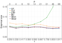
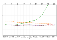
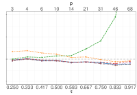
Figure S5: Empirical size for the directional test (DT), central limit theorem test (CLT), likelihood ratio test (LRT), Bartlett correction (BC) and two Skovgaard,’s modifications (Sko1 and Sko2) for hypothesis (8) in the paper, at nominal level $\alpha=0.05$ given by the gray horizontal line. The left, middle and right panels correspond to multivariate $t$, multivariate skew-normal, and multivariate Laplace distributions of the true generating process, respectively, with $n_{i}=100$ and $g=3$.

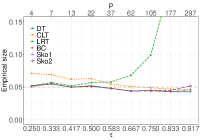
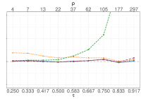
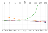
Figure S6: Empirical size for the directional test (DT), central limit theorem test (CLT), likelihood ratio test (LRT), Bartlett correction (BC) and two Skovgaard,’s modifications (Sko1 and Sko2, respectively) for hypothesis (8) in the paper, at nominal level $\alpha=0.05$ given by the gray horizontal line. The left, middle and right panels correspond to multivariate $t$, multivariate skew-normal, and multivariate Laplace distributions of the true generating process, respectively, with $n_{i}=500$ and $g=3$.

Table S5: Empirical size of the directional test (DT), central limit theorem test (CLT), likelihood ratio test (LRT), Bartlett correction (BC) and two Skovgaard,’s modifications (Sko1 and Sko2) for hypothesis (8) in the paper with $p=n_{i}^{\tau}$ and $n_{i}=100$ and $g=3$, at nominal level $\alpha=0.05$.

True Distribution	$\tau$ ($p$)	DT	CLT	LRT	BC	Sko1	Sko2
Multivariate $t$	0.250 (3)	0.050	0.069	0.053	0.050	0.049	0.049
	0.333 (4)	0.044	0.063	0.048	0.044	0.042	0.042
	0.417 (6)	0.048	0.065	0.054	0.048	0.047	0.047
	0.500 (10)	0.047	0.059	0.055	0.046	0.045	0.045
	0.583 (14)	0.050	0.060	0.064	0.050	0.049	0.048
	0.667 (21)	0.049	0.061	0.075	0.049	0.048	0.048
	0.750 (31)	0.044	0.054	0.096	0.045	0.043	0.043
	0.833 (46)	0.042	0.049	0.148	0.043	0.041	0.040
	0.917 (68)	0.042	0.047	0.302	0.047	0.045	0.041
Multivariate skew-normal	0.250 (3)	0.050	0.070	0.053	0.050	0.049	0.049
	0.333 (4)	0.050	0.070	0.055	0.050	0.050	0.049
	0.417 (6)	0.047	0.064	0.053	0.047	0.046	0.046
	0.500 (10)	0.050	0.062	0.059	0.050	0.048	0.048
	0.583 (14)	0.051	0.064	0.068	0.051	0.049	0.049
	0.667 (21)	0.048	0.059	0.076	0.048	0.046	0.045
	0.750 (31)	0.048	0.057	0.100	0.048	0.047	0.046
	0.833 (46)	0.050	0.057	0.159	0.052	0.049	0.048
	0.917 (68)	0.049	0.055	0.312	0.054	0.052	0.048
Multivariate Laplace	0.250 (3)	0.048	0.067	0.050	0.048	0.046	0.046
	0.333 (4)	0.051	0.069	0.055	0.051	0.050	0.050
	0.417 (6)	0.047	0.064	0.054	0.048	0.046	0.046
	0.500 (10)	0.047	0.061	0.057	0.047	0.046	0.046
	0.583 (14)	0.043	0.054	0.058	0.043	0.042	0.042
	0.667 (21)	0.044	0.055	0.073	0.044	0.043	0.043
	0.750 (31)	0.042	0.049	0.091	0.043	0.040	0.040
	0.833 (46)	0.038	0.044	0.145	0.040	0.038	0.036
	0.917 (68)	0.039	0.046	0.301	0.045	0.042	0.038

Table S6: Empirical size of the directional test (DT), central limit theorem test (CLT), likelihood ratio test (LRT), Bartlett correction (BC) and two Skovgaard,’s modifications (Sko1 and Sko2) for hypothesis (8) in the paper with $p=n_{i}^{\tau}$ and $n_{i}=500$ and $g=3$, at nominal level $\alpha=0.05$.

True Distribution	$\tau$ ($p$)	DT	CLT	LRT	BC	Sko1	Sko2
Multivariate $t$	0.250 (4)	0.052	0.071	0.052	0.052	0.051	0.051
	0.333 (7)	0.055	0.069	0.057	0.055	0.055	0.055
	0.417 (13)	0.050	0.062	0.052	0.050	0.050	0.050
	0.500 (22)	0.052	0.063	0.057	0.052	0.051	0.051
	0.583 (37)	0.048	0.055	0.058	0.048	0.048	0.048
	0.667 (62)	0.044	0.051	0.068	0.044	0.044	0.044
	0.750 (105)	0.045	0.049	0.099	0.045	0.045	0.044
	0.833 (177)	0.043	0.047	0.212	0.045	0.045	0.043
	0.917 (297)	0.043	0.046	0.618	0.052	0.052	0.046
Multivariate skew-normal	0.250 (4)	0.051	0.069	0.052	0.051	0.051	0.051
	0.333 (7)	0.052	0.068	0.053	0.052	0.051	0.051
	0.417 (13)	0.051	0.062	0.053	0.050	0.050	0.050
	0.500 (22)	0.049	0.058	0.054	0.049	0.049	0.049
	0.583 (37)	0.051	0.060	0.062	0.051	0.050	0.050
	0.667 (62)	0.052	0.058	0.076	0.052	0.052	0.052
	0.750 (105)	0.055	0.058	0.108	0.055	0.055	0.054
	0.833 (177)	0.048	0.051	0.218	0.049	0.049	0.048
	0.917 (297)	0.051	0.054	0.612	0.058	0.058	0.053
Multivariate Laplace	0.250 (4)	0.048	0.067	0.050	0.048	0.048	0.048
	0.333 (7)	0.053	0.069	0.054	0.053	0.052	0.052
	0.417 (13)	0.049	0.063	0.053	0.049	0.049	0.049
	0.500 (22)	0.046	0.056	0.051	0.047	0.046	0.046
	0.583 (37)	0.048	0.054	0.056	0.048	0.048	0.048
	0.667 (62)	0.046	0.054	0.070	0.046	0.046	0.046
	0.750 (105)	0.045	0.050	0.099	0.046	0.045	0.044
	0.833 (177)	0.041	0.045	0.209	0.043	0.042	0.041
	0.917 (297)	0.037	0.039	0.609	0.043	0.043	0.038

Appendix S2 Simulation studies for Heteroscedastic one-way MANOVA

This section is studied the performance of directional test for heteroscedastic one-way MANOVA, comparing with LRT, Sko1 and Sko1. In particular, when the number of groups $g=2$, we also consider the $F$-approximation for the Behrens-Fisher test $T^{*2}$. The simulation results are computed via Monte Carlo simulation based on 10,000 replications.

S2.1 Empirical results for the moderate setup

Groups of size $n_{i},i\in\{1,\dots,g\}$, are generated from a $p$-variate standard normal distribution $N_{p}(0_{p},\Lambda_{i}^{-1})$ under the null hypothesis. We use an autoregressive structure for the covariance matrices. i.e. $\Lambda_{i}^{-1}=(\sigma_{jl})_{p\times p}=(\rho_{i}^{|j-l|})_{p\times p}$, with the $\rho_{i}$ chosen to an equally-distance sequence from 0.1 to 0.9 of length $g$. For each simulation experiment, we show results for $p=\lceil n_{i}^{\tau}\rceil$ with $\tau=j/24$, $j\in\{6,7,\cdots,22\}$ and $n_{i}\in\{100,500,1000\}$ and $k=2$.

Table S7: Empirical size of the directional test (DT), Behrens-Fisher test (BF) (Nel and Merwe,, 1986), likelihood ratio test (LRT), and two Skovgaard,’s modifications (Sko1 and Sko2) for hypothesis (9) in the paper with $p=n_{i}^{\tau}$ and $n_{i}=100,500,1000$, at nominal level $\alpha=0.05$.

$n_{i}$	$\tau$ ($p$)	DT	BF	LRT	Sko1	Sko2
100	0.250 (4)	0.053	0.054	0.057	0.053	0.053
	0.333 (5)	0.050	0.052	0.056	0.050	0.050
	0.417 (7)	0.049	0.051	0.057	0.050	0.050
	0.500 (10)	0.051	0.056	0.065	0.052	0.052
	0.583 (15)	0.052	0.061	0.077	0.052	0.052
	0.667 (22)	0.049	0.065	0.094	0.051	0.050
	0.750 (32)	0.051	0.082	0.147	0.055	0.053
	0.833 (47)	0.052	0.115	0.270	0.067	0.061
	0.917 (69)	0.064	0.183	0.594	0.112	0.092
500	0.250 (5)	0.050	0.050	0.051	0.050	0.050
	0.333 (8)	0.051	0.051	0.052	0.051	0.051
	0.417 (14)	0.051	0.052	0.055	0.051	0.051
	0.500 (23)	0.051	0.054	0.059	0.051	0.051
	0.583 (38)	0.054	0.061	0.070	0.054	0.054
	0.667 (63)	0.051	0.068	0.089	0.052	0.052
	0.750 (106)	0.048	0.084	0.143	0.051	0.050
	0.833 (178)	0.051	0.154	0.382	0.062	0.058
	0.917 (298)	0.060	0.392	0.923	0.137	0.106
1000	0.250 (6)	0.052	0.052	0.053	0.052	0.052
	0.333 (10)	0.050	0.050	0.051	0.050	0.050
	0.417 (18)	0.046	0.048	0.048	0.046	0.046
	0.500 (32)	0.052	0.055	0.058	0.052	0.052
	0.583 (57)	0.052	0.058	0.063	0.052	0.052
	0.667 (100)	0.050	0.066	0.083	0.050	0.050
	0.750 (178)	0.047	0.088	0.154	0.050	0.049
	0.833 (317)	0.051	0.179	0.459	0.065	0.059
	0.917 (563)	0.064	0.528	0.987	0.155	0.112

S2.2 Robustness to misspecification

Table S8: Empirical size of the directional test (DT), Behrens-Fisher test (BF) (Nel and Merwe,, 1986), likelihood ratio test (LRT), and two Skovgaard,’s modifications (Sko1 and Sko2) for hypothesis (9) in the paper with $p=n_{i}^{\tau}$ and $n_{i}=100$ and $g=2$, at nominal level $\alpha=0.05$.

Distribution	$\tau$ ($p$)	DT	BF	LRT	Sko1	Sko2
Multivariate $t$	0.250 (4)	0.048	0.048	0.052	0.048	0.048
	0.333 (5)	0.047	0.047	0.053	0.047	0.047
	0.417 (7)	0.048	0.048	0.055	0.048	0.048
	0.500 (10)	0.050	0.049	0.060	0.050	0.050
	0.583 (15)	0.045	0.044	0.064	0.045	0.045
	0.667 (22)	0.047	0.046	0.078	0.047	0.047
	0.750 (32)	0.042	0.040	0.102	0.043	0.042
	0.833 (47)	0.041	0.038	0.166	0.044	0.042
	0.917 (69)	0.043	0.038	0.375	0.054	0.048
Multivariate skew-normal	0.250 (4)	0.046	0.046	0.051	0.046	0.046
	0.333 (5)	0.052	0.052	0.058	0.052	0.052
	0.417 (7)	0.053	0.053	0.061	0.053	0.053
	0.500 (10)	0.054	0.054	0.064	0.054	0.054
	0.583 (15)	0.049	0.049	0.070	0.050	0.049
	0.667 (22)	0.048	0.047	0.080	0.048	0.048
	0.750 (32)	0.050	0.048	0.110	0.051	0.050
	0.833 (47)	0.052	0.051	0.187	0.056	0.053
	0.917 (69)	0.048	0.048	0.379	0.061	0.053
Multivariate Laplace	0.250 (4)	0.049	0.049	0.054	0.049	0.049
	0.333 (5)	0.044	0.044	0.050	0.044	0.044
	0.417 (7)	0.045	0.045	0.051	0.045	0.045
	0.500 (10)	0.046	0.046	0.055	0.046	0.045
	0.583 (15)	0.045	0.045	0.063	0.045	0.045
	0.667 (22)	0.044	0.043	0.075	0.044	0.044
	0.750 (32)	0.040	0.039	0.097	0.042	0.040
	0.833 (47)	0.039	0.038	0.169	0.043	0.040
	0.917 (69)	0.034	0.032	0.372	0.044	0.038

Table S9: Empirical size of the directional test (DT), Behrens-Fisher test (BF) (Nel and Merwe,, 1986), likelihood ratio test (LRT), and two Skovgaard,’s modifications (Sko1 and Sko2) for hypothesis (9) in the paper with $p=n_{i}^{\tau}$ and $n_{i}=500$ and $g=2$, at nominal level $\alpha=0.05$.

Distribution	$\tau$ ($p$)	DT	BF	LRT	Sko1	Sko2
Multivariate $t$	0.250 (5)	0.050	0.050	0.052	0.050	0.050
	0.333 (8)	0.049	0.049	0.050	0.049	0.049
	0.417 (14)	0.047	0.047	0.050	0.047	0.047
	0.500 (23)	0.045	0.045	0.050	0.045	0.045
	0.583 (38)	0.051	0.051	0.063	0.051	0.051
	0.667 (63)	0.044	0.044	0.070	0.044	0.044
	0.750 (106)	0.044	0.043	0.108	0.044	0.044
	0.833 (178)	0.044	0.043	0.236	0.048	0.046
	0.917 (298)	0.047	0.045	0.705	0.064	0.053
Multivariate skew-normal	0.250 (5)	0.051	0.051	0.052	0.051	0.051
	0.333 (8)	0.051	0.051	0.052	0.051	0.051
	0.417 (14)	0.055	0.055	0.059	0.055	0.055
	0.500 (23)	0.054	0.054	0.060	0.054	0.054
	0.583 (38)	0.051	0.051	0.061	0.051	0.051
	0.667 (63)	0.049	0.049	0.074	0.049	0.049
	0.750 (106)	0.051	0.051	0.117	0.052	0.052
	0.833 (178)	0.048	0.048	0.242	0.054	0.050
	0.917 (298)	0.052	0.051	0.699	0.070	0.058
Multivariate Laplace	0.250 (5)	0.054	0.054	0.054	0.053	0.053
	0.333 (8)	0.053	0.053	0.054	0.053	0.053
	0.417 (14)	0.050	0.050	0.052	0.050	0.050
	0.500 (23)	0.051	0.051	0.056	0.051	0.051
	0.583 (38)	0.047	0.047	0.056	0.047	0.047
	0.667 (63)	0.046	0.046	0.070	0.047	0.046
	0.750 (106)	0.042	0.042	0.106	0.043	0.043
	0.833 (178)	0.040	0.040	0.235	0.043	0.040
	0.917 (298)	0.033	0.032	0.708	0.051	0.040

S2.3 Empirical results for large number $k$ of groups

Table S10: Empirical size of the directional test (DT), likelihood ratio test (LRT), and two Skovgaard,’s modifications (Sko1 and Sko2) for hypothesis (9) in the paper with $p=n_{i}^{\tau}$ and $n_{i}=100$ and $g=30$, at nominal level $\alpha=0.05$.

$\tau$ ($p$)	DT	LRT	Sko1	Sko2
0.250 (4)	0.050	0.081	0.050	0.050
0.333 (5)	0.050	0.091	0.050	0.050
0.417 (7)	0.049	0.122	0.050	0.049
0.500 (10)	0.050	0.186	0.051	0.050
0.583 (15)	0.054	0.391	0.058	0.054
0.667 (22)	0.047	0.751	0.056	0.048
0.750 (32)	0.052	0.990	0.087	0.062
0.833 (47)	0.049	1.000	0.223	0.095
0.917 (69)	0.048	1.000	0.932	0.405

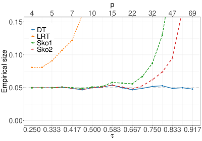
Figure S7: Empirical size of the directional test (DT), likelihood ratio test (LRT), and two Skovgaard,’s modifications (Sko1 and Sko2) for hypothesis (9) in the paper with $p=n_{i}^{\tau}$ and $n_{i}=100$ and $g=30$, at nominal level $\alpha=0.05$ given by the gray horizontal line.

Table S11: Empirical size of the directional test (DT), likelihood ratio test (LRT), and two Skovgaard,’s modifications (Sko1 and Sko2) for hypothesis (9) in the paper with $p=n_{i}^{\tau}$ and $n_{i}=1000$ and $g=5$, at nominal level $\alpha=0.05$

$\tau$ ($p$)	DT	LRT	Sko1	Sko2
0.250 (6)	0.053	0.055	0.053	0.053
0.333 (10)	0.055	0.058	0.055	0.055
0.417 (18)	0.048	0.054	0.048	0.048
0.500 (32)	0.048	0.061	0.048	0.048
0.583 (57)	0.051	0.089	0.052	0.052
0.667 (100)	0.054	0.160	0.055	0.054
0.750 (178)	0.053	0.462	0.058	0.055
0.833 (317)	0.050	0.983	0.083	0.063

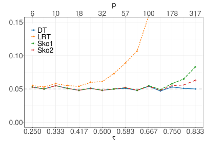
Figure S8: Empirical size of the directional test (DT), likelihood ratio test (LRT), and two Skovgaard,’s modifications (Sko1 and Sko2) for hypothesis (9) in the paper, with $p=n_{i}^{\tau}$ and $n_{i}=1000$ and $g=5$, at nominal level $\alpha=0.05$ given by the gray horizontal line.

References

- Azzalini and Capitanio, (1999) Azzalini, A. and Capitanio, A. (1999). Statistical applications of the multivariate skew normal distribution. Journal of the Royal Statistical Society: Series B (Statistical Methodology), 61:579–602.
- Bartlett, (1937) Bartlett, M. (1937). Properties of sufficiency and statistical tests. Proceedings of the Royal Society of London. Series A-Mathematical and Physical Sciences, 160:268–282.
- Bate et al., (2023) Bate, D., Maechler, M., Jagan, M., Davis, T. A., Oehlschlägel, J., Riedy, J., and Team, R. C. (2023). Matrix: Sparse and Dense Matrix Classes and Methods. R package version 0.3.5.
- Battey and Cox, (2022) Battey, H. and Cox, D. (2022). Some perspectives on inference in high dimensions. Statistical Science, 37:110–122.
- Davison et al., (2014) Davison, A. C., Fraser, D. A. S., Reid, N., and Sartori, N. (2014). Accurate directional inference for vector parameters in linear exponential families. Journal of the American Statistical Association, 109:302–314.
- Davison and Reid, (2022) Davison, A. C. and Reid, N. (2022). The tangent exponential model. arXiv preprint arXiv:2106.10496v2.
- Di Caterina et al., (2023) Di Caterina, C., Reid, N., and Sartori, N. (2023). Accurate directional inference in Gaussian graphical models. Statistica Sinica, to appear. doi:10.5705/ss.202022.0394.
- Fox et al., (2022) Fox, J., Weisberg, S., Price, B., Adler, D., Bates, D., Baud-Bovy, G., Bolker, B., Ellison, S., Firth, D., Friendly, M., and so on (2022). car: Companion to Applied Regression. R package version 0.3.1.
- Fraser et al., (2016) Fraser, D. A. S., Reid, N., and Sartori, N. (2016). Accurate directional inference for vector parameters. Biometrika, 103:625–639.
- He et al., (2021) He, Y., Meng, B., Zeng, Z., and Xu, G. (2021). On the phase transition of Wilks’ phenomenon. Biometrika, 108:741–748.
- Huang et al., (2022) Huang, C., Di Caterina, C., and Sartori, N. (2022). Directional testing for high-dimensional multivariate normal distributions. Electronic Journal of Statistics, 16:6489–6511.
- Jiang and Yang, (2013) Jiang, T. and Yang, F. (2013). Central limit theorems for classical likelihood ratio tests for high-dimensional normal distributions. The Annals of Statistics, 41:2029–2074.
- Lauritzen, (1996) Lauritzen, S. L. (1996). Graphical Models. Oxford University Press.
- Magnus and Neudecker, (1999) Magnus, J. and Neudecker, H. (1999). Matrix Differential Calculus with Applications in Statistics and Econometrics. Wiley, 3ed edition.
- McCormack et al., (2019) McCormack, A., Reid, N., Sartori, N., and Theivendran, S. A. (2019). A directional look at -tests. Canadian Journal of Statistics, 47:619–627.
- McCullagh, (2018) McCullagh, P. (2018). Tensor Methods in Statistics. Dover Publications, 2nd edition.
- Nel and Merwe, (1986) Nel, D. and Merwe, C. V. D. (1986). A solution to the multivariate Behrens-Fisher problem. Communications in Statistics - Theory and Methods, 15:3719–3735.
- Pace and Salvan, (1997) Pace, L. and Salvan, A. (1997). Principles of Statistical Inference from a Neo-Fisherian Perspective. World Scientific Press.
- R Core Team, (2023) R Core Team (2023). R: A Language and Environment for Statistical Computing. R Foundation for Statistical Computing, Vienna, Austria.
- Rencher, (1998) Rencher, A. C. (1998). Multivariate Statistical Inference and Applications. Wiley-Interscience.
- Sartori, (2017) Sartori, N. (2017). Introduction to “Saddlepoint Expansions for Directional Test Probabilities”. In Inference, Asymptotics, and Applications. Selected Papers of Ib Michael Skovgaard, with Introductions by his Colleagues (Reid and Martinussen Eds). World Scientific.
- Skovgaard, (1988) Skovgaard, I. (1988). Saddlepoint expansions for directional test probabilities. Journal of the Royal Statistical Society, Series B (Statistical Methodology), 50:269–280.
- Skovgaard, (2001) Skovgaard, I. (2001). Likelihood asymptotics. Scandinavian Journal of Statistics, 28:3–32.
- Sur et al., (2019) Sur, P., Chen, Y., and Candès, E. J. (2019). The likelihood ratio test in high-dimensional logistic regression is asymptotically a rescaled chi-square. Probability theory and related fields, 175:487–558.
- Tang and Reid, (2020) Tang, Y. and Reid, N. (2020). Modified likelihood root in high dimensions. Journal of the Royal Statistical Society: Series B (Statistical Methodology), 82:1349–1369.
- Tang and Reid, (2021) Tang, Y. and Reid, N. (2021). Laplace and saddlepoint approximations in high dimensions. arXiv preprint arXiv:2107.10885.