Discrete Laplacian thermostat for flocks and swarms: the fully conserved
Inertial Spin Model

Abstract

Experiments on bird flocks and midge swarms reveal that these natural systems are well described by an active theory in which conservation laws play a crucial role. By building a symplectic structure that couples the particles’ velocities to the generator of their internal rotations (spin), the Inertial Spin Model (ISM) reinstates a second-order temporal dynamics that captures many phenomenological traits of flocks and swarms. The reversible structure of the ISM predicts that the total spin is a constant of motion, the central conservation law responsible for all the novel dynamical features of the model. However, fluctuations and dissipation introduced in the original model to make it relax, violate the spin conservation law, so that the ISM aligns with the biophysical phenomenology only within finite-size regimes, beyond which the overdamped dynamics characteristic of the Vicsek model takes over. Here, we introduce a novel version of the ISM, in which the irreversible terms needed to relax the dynamics strictly respect the conservation of the spin. We perform a numerical investigation of the fully conservative model, exploring both the fixed-network case, which belongs to the equilibrium class of Model G, and the active case, characterized by self-propulsion of the agents and an out-of-equilibrium reshuffling of the underlying interaction network. Our simulations not only capture the correct spin wave phenomenology of the ordered phase, but they also yield dynamical critical exponents in the near-ordering phase that agree very well with the theoretical predictions.

I Introduction

Approximately three decades ago, Vicsek and coworkers enlisted a sizeable number of unwilling statistical physicists into the fast-growing field of biophysics by introducing a simple little model that captured elegantly the key traits of collective animal behaviour Vicsek et al. (1995). This model, partly rooted in the physics of ferromagnets and critical phenomena, partly drawing inspiration from previous efforts in the field of computer graphics Reynolds (1987), demonstrated that local alignment could induce collective motion and long-range correlations even in active systems; in fact, the Vicsek model showed that activity favours order, allowing for a coherent (or flocking) phase also in two dimensions Toner and Tu (1995), where equilibrium physics would prevent long-range ordering. Under more than one respect (but not all respects), this was the start of active matter physics Ramaswamy (2010); Ginelli (2016); Chaté (2020).

Vicsek’s model is truly remarkable for its simplicity and great generality, so much so that it can be considered the Ising model of active matter. However, as soon as experimental data on actual biological groups started to flow in, it was clear that the quantitative description of certain biological features required models to incorporate some additional elements. Among the many variants and evolutions of the Vicsek model aimed at better describing biological reality Tu et al. (1998a); Grégoire and Chaté (2004); Chaté et al. (2008, 2008); Moreno et al. (2020); Chaté (2020); Chepizhko et al. (2021), one in particular is of interest for us here: the so-called Inertial Spin Model (ISM) Attanasi et al. (2014a); Cavagna et al. (2015).

Observations on starling flocks revealed that collective information during turns propagates linearly and nearly undamped throughout the group Attanasi et al. (2014a). Not much later, experiments on natural swarms of midges showed that the dynamical correlation functions display unmistakable traits of inertial relaxation Cavagna et al. (2017); at the same time, swarms have a dynamical critical exponent lower than any other reference ferromagnetic model, and (worse) of the very Vicsek model Cavagna et al. (2017, 2023a). All these traits prompted to develop a new model in which the inertial features of the dynamics — washed out in the Vicsek model — were reinstated, giving rise to a conservation law able to account for several new biological pieces of phenomenology. This model is the ISM, developed in Attanasi et al. (2014a); Cavagna et al. (2015) and further studied in Ha et al. (2019); Markou (2021); Benedetto et al. (2020); Ko et al. (2023); Huh and Kim (2022), the overdamped limit of which is — notably — the Vicsek model.

The ISM successfully reproduces several traits of natural flocks and swarms, including: the linear propagation law of orientational waves in bird flocks, even in density-homogeneous systems Attanasi et al. (2014a); the quantitative dependence of the speed of propagation of these waves on polarization Attanasi et al. (2014a); the precise inertial shape of the dynamical correlation functions in midge swarms Cavagna et al. (2017); dynamic scaling laws Cavagna et al. (2017); and finally the precise prediction of the dynamical critical exponent in natural swarms Cavagna et al. (2023a), perhaps the only instance to date of agreement between theory, experiments and numerics on a critical exponent of an actual biological system. But the ISM has an issue: despite the fact that its founding pillar is the spin conservation law, the ISM has in fact no way to exactly respect that very conservation law, which is somewhat annoying.

The reason why that happens is simple. The conservation law of the ISM stems from its novel reversible dynamics, which reinstates the symplectic structure between generalized coordinate and conjugated momentum. However, in order to turn this structure into a relaxational statistical model, one needs to introduce fluctuation-dissipation terms (noise and friction, essentially), which — in their current form — violate the conservation law. This means that up to now the ISM was able to reproduce underdamped inertial dynamics only in finite-size systems and for small friction (the two things are related; see below). Although practically acceptable and in line with the experimental observations, from a purely theoretical point of view this is unpleasant; it would be important to have a model which can relax and at the same time respect the conservation law responsible for the new physics, irrespective of the system’s size. Here, we present a solution to this problem.

II The fully-conserved Inertial Spin Model

II.1 Deterministic structure

The novelty of the model we are going to introduce will be in the new kind of irreversible and yet conservative terms. However, in order to better understand the evolution from one model to another, it is better to start our discussion from the — rather unphysical — purely deterministic cases and to gradually build up later noise and dissipation.

For all the self-propelled models described in this work the first equation of motion is $\dot{\boldsymbol{r}}_{i}=\boldsymbol{v}_{i}$, hence we will not repeat it every time; if/when we will consider the fixed-network version of a model, we will simply set $\dot{\boldsymbol{r}}_{i}=0$. The equation for the velocity, on the other hand, defines the particular model; we will start from the simplest one, that is Vicsek.

II.1.1 The Vicsek rule

In what follows we will consider fixed modulus of the velocity, and to simplify the notation we will set $|\boldsymbol{v}_{i}|=1$ (the reader should be careful then in comparing with the previous literature, where the fixed value of the speed is often left as a dimensional parameter, $v_{0}$). In its barest, deterministic form, the Vicsek dynamics Vicsek et al. (1995), can be written as,

$$\eta\frac{d\boldsymbol{v}_{i}}{dt}=\left(\boldsymbol{v}_{i}\times J\sum_{j}n_{ij}\boldsymbol{v}_{j}\right)\times\boldsymbol{v}_{i}\ ,$$ (1)

where $J$ corresponds to the alignment strength and $n_{ij}$ is the adjacency matrix ($n_{ij}=1$ if the agents $i$ and $j$ interact, $n_{ij}=0$ otherwise – as we shall see later on the specific interaction rule (metric vs. topological) may depend on the system under consideration Cavagna et al. (2018)). Of course, in the active case where the equation $\dot{\boldsymbol{r}}_{i}=\boldsymbol{v}_{i}$ is at work, the adjacency matrix depends on time, $n_{ij}=n_{ij}(t)$, which is the essence of the out-of-equilibrium nature of self-propelled particles models.

The funny double cross product structure is simply a compact way to conserve the modulus of $\boldsymbol{v}_{i}$ under the Vicsek dynamics: the neighbours of agent $i$ exert a so-called social force, $\boldsymbol{f}_{i}=J\sum_{j}n_{ij}\boldsymbol{v}_{j}$; the term $(\boldsymbol{v}_{i}\times\boldsymbol{f}_{i})\times\boldsymbol{v}_{i}$ is simply the projection of $\boldsymbol{f}_{i}$ onto the plane orthogonal to $\boldsymbol{v}_{i}$, namely $\boldsymbol{f}_{i}^{\perp}$. In this way, the effect of the Vicsek rule is to rotate particle $i$’s velocity towards the social force, i.e. towards the average direction of motion of its neighbours; the way this happens is direct: the force $\boldsymbol{f}_{i}$ rotates the velocity $\boldsymbol{v}_{i}$ through the double cross product. This alignment rule creates an overdamped dynamics for the velocity, which is exactly what the ISM wants to change. Note that we have explicitly left the dissipation parameter $\eta$ in the equation, which at this level simply defines a time scale; although usually eliminated by rescaling time in the Vicsek model, it will be convenient to keep it for a comparison with the ISM in what follows.

II.1.2 The Inertial Spin Model rule

The key idea of the ISM — compared to the Vicsek model — is that the social alignment force produced by an agent’s neighbours, instead of rotating directly the velocity of the agent, acts on its spin, which is the generator of the rotations of the velocity; it is the spin that, in turns, rotates the velocity, according to the equations Cavagna et al. (2015),

$$\frac{d\boldsymbol{v}_{i}}{dt} =\frac{1}{\chi}\boldsymbol{s}_{i}\times\boldsymbol{v}_{i},$$ (2a)

$$\frac{d\boldsymbol{s}_{i}}{dt} =\boldsymbol{v}_{i}\times J\sum_{j}n_{ij}\boldsymbol{v}_{j}\ .$$ (2b)

This symplectic relationship between velocity and spin is the same as — for example — that between position and angular momentum, when rotations in the external space are considered; from this analogy we clearly see that the parameter $\chi$ acts as a generalized inertia, i.e. a al or physiological resistance of the agents to rotate their direction of motion. To simplify things at their core, we could say that the ISM equations are to the velocity, what the standard equations of rotational motion are to the position,

$$\frac{d\boldsymbol{r}}{dt} =\frac{1}{I}\ \boldsymbol{l}\times\boldsymbol{r}$$

$$\frac{d\boldsymbol{l}}{dt} =\boldsymbol{r}\times\boldsymbol{F}$$

where $\boldsymbol{l}$ is the angular momentum, $I$ is the moment of inertia and $\boldsymbol{F}$ is the force (the constraint of fixed speed in the ISM is analogous to the constraint of fixed radius within rotational motion).

The crucial point is that, if the interaction ruling the dynamics is symmetric under a given transformation, a global conservation law emerges due to Noether’s teorem. This is exactly the case of the alignment interaction of self-propelled models: the social force $\boldsymbol{f}_{i}$ is invariant under rotation of the velocity (readers can check that), so that — once the symplectic structure of velocity and spin is restored — the generator of rotations, namely the total spin of the system, in absence of dissipative forces, is a constant of motion. This conservation law is a game-changer: in the ordered phase of the ISM it is the cause of the emergence of linear spin waves observed in actual biological flocks Attanasi et al. (2014a), while in the near-ordering phase it accounts for much of the dynamical phenomenology of natural swarms of insects, including inertial dynamic relaxation Cavagna et al. (2017) and an anomalous dynamical critical exponent Cavagna et al. (2023a).

II.2 Stochastic structure

II.2.1 Adding fluctuation and dissipation

All these models, of course, must be complemented with some noise, accounting for the obvious fact that biological agents are unlikely to obey whatever effective interaction rule in a perfect deterministic way and (most importantly) allowing the relaxation of the dynamics. For the Vicsek rule the task is quite simple: we simply add to the r.h.s. of (1) a noise term, being careful to preserve the constraint $|\boldsymbol{v}_{i}|=1$. One possible way to do this is the following,

$$\eta\frac{d\boldsymbol{v}_{i}}{dt}=\left(\boldsymbol{v}_{i}\times J\sum_{j}n_{ij}\boldsymbol{v}_{j}\right)\times\boldsymbol{v}_{i}+\boldsymbol{\xi}_{i}\times\boldsymbol{v}_{i}\ .$$ (3)

where $\boldsymbol{\xi}_{i}$ is a white noise with correlator,

$$\langle\xi_{i}^{\mu}(t)\xi_{j}^{\nu}(t^{\prime})\rangle=2\eta T\ \delta(t-t^{\prime})\delta_{ij}\delta^{\mu\nu}\ .$$ (4)

The choice of noise in (3) is not the only possibility; another (and perhaps more intuitive) choice would be to add a stochastic term of the form, $\boldsymbol{v}_{i}\times(\boldsymbol{\xi}_{i}\times\boldsymbol{v}_{i})=\boldsymbol{\xi}_{i}^{\perp}$, similarly to what happens to the force; that is the way in which the continuous-time Vicsek model is written in Cavagna et al. (2015). In fact, both types of noise conserve the modulus of the velocity and have the same exact correlator, given by the projector orthogonal to the velocity; hence from the practical point of view it makes no difference, but the form in (3) is more convenient because (as we shall see in a minute), it will appear naturally when we will take the overdamped limit of the inertial model.

Within the ISM, given that we have two equations, we need to be more careful: where are we going to add the noise? Because noise is a stochastic (generalized) force and forces act in general on the time derivative of the conjugate momentum to the coordinate (in this case, the velocity is an internal coordinate), it is reasonable to add noise to the second equation of (2); moreover, it is natural to associate to each noise force (fluctuation), an irreversible force causing relaxation (dissipation), again in the equation for the conjugate momentum. If we follow this scheme in adding fluctuation-dissipation to (2), we obtain the ISM equations,

$$\frac{d\boldsymbol{v}_{i}}{dt} =\frac{1}{\chi}\boldsymbol{s}_{i}\times\boldsymbol{v}_{i},$$ (5a)

$$\frac{d\boldsymbol{s}_{i}}{dt} =\boldsymbol{v}_{i}\times J\sum_{j}n_{ij}\boldsymbol{v}_{j}-\frac{\eta}{\chi}\boldsymbol{s}_{i}+\boldsymbol{\xi}_{i},$$ (5b)

again with,

$$\langle\xi_{i}^{\mu}(t)\xi_{j}^{\nu}(t^{\prime})\rangle=2\eta T\ \delta(t-t^{\prime})\delta_{ij}\delta^{\mu\nu}.$$ (6)

We notice that – because the noise is now in the equation for the spin – there is no need to cross-product it with the velocity to keep the norm of $\boldsymbol{v}_{i}$ fixed, as the equation for the velocity automatically does that. The dissipation and noise are the irreversible terms that allow the system to relax towards a non-equilibrium stationary state. The nice thing about this structure is that the overdamped limit of this model (very large $\eta$) corresponds to the Vicsek model. To be more precise, the overdamped limit is always a limit in time; the inertial time scale of the system is $\chi/\eta$, hence the overdamped limit corresponds to $\eta$ so large that the inertial scale is shorter than the microscopic time scale of the system (as the inertial $\chi$ is always an innocuous parameter of order $1$, the overdamped limit is often identified as that of large $\eta$). In this regime, the spin becomes a fast variable, so we can set $\dot{\boldsymbol{s}}_{i}=0$, and get,

$$\frac{\eta}{\chi}\boldsymbol{s}_{i}=\boldsymbol{v}_{i}\times J\sum_{j}n_{ij}\boldsymbol{v}_{j}+\boldsymbol{\xi}_{i}\ ,$$ (7)

which, once plugged into the equation for $\dot{\boldsymbol{v}}_{i}$, yields,

$$\eta\frac{d\boldsymbol{v}_{i}}{dt}=\left(\boldsymbol{v}_{i}\times J\sum_{j}n_{ij}\boldsymbol{v}_{j}+\boldsymbol{\xi}_{i}\right)\times\boldsymbol{v}_{i}\ ,$$ (8)

which is exactly the Vicsek model, (3). From the conceptual point of view, this is particularly pleasing: the ISM is not some completely new model that has nothing to do with Vicsek; the ISM is simply the underdamped version of the Vicsek model. Or – more accurately – the Vicsek model is the overdamped limit of the ISM. Also, in this way we better understand where the parameter $\eta$ in the Vicsek model comes from.

An important technical point is in order. The equation for the spin in (5) is subtly different from (and simpler than) the corresponding ISM equation first introduced in Cavagna et al. (2015). The reason is the following. In the original model it was imposed the constraint $\boldsymbol{s}_{i}\cdot\boldsymbol{v}_{i}=0$, which required that both the dissipative term and the noise term in the spin dynamics had to be crossed-multiplied by $\boldsymbol{v}_{i}$. The purpose of the present work, though, is to add a conservative irreversible structure to the model, which can make it stochastic while conserving the total spin; as we shall see later on, the new conservative terms will violate the strict condition $\boldsymbol{s}_{i}\cdot\boldsymbol{v}_{i}=0$ (although it will still hold on average). Because of this, we find it more convenient to relax the constraint from the outset also in the original case of standard dissipation, thus introducing this slightly simpler version of the ISM, equation (5), which is the one we will actually generalize to the conservative case. From the physical point if view, the noise in equation (5) corresponds to the case in which the system is directly exchanging spin with the environment, while the original ISM equations of Cavagna et al. (2015) correspond to the case in which the system stochastically exchanges with the environment the linear generator, $\boldsymbol{w}_{i}$, with $\boldsymbol{s}_{i}=\boldsymbol{v}_{i}\times\boldsymbol{w}_{i}$ Carruitero et al. (2023). Because the ISM is an effective model, with no direct connection with the actual mechanics of the agents described, and because we have no idea of the actual interaction with the environment considered as a heat bath, both descriptions are acceptable, depending on the desired applications of the model. We notice, though, that once we give up the constraint $\boldsymbol{s}_{i}\cdot\boldsymbol{v}_{i}=0$, we can no longer work on the ISM within the framework of the linear generator $\boldsymbol{w}_{i}$, as it was recently done in Carruitero et al. (2023).

II.2.2 The issue of dissipation and the RG crossover

The route from an underdamped model for low $\eta$ to an overdamped one for large $\eta$ has a particularly clear and vivid representation in the context of the Renormalization Group (RG), where the two limits are described by two different asymptotic fixed points Cavagna et al. (2023a). The crucial concept, though, is that in the vicinity of the underdamped fixed point ($\eta=0$), dissipation is a relevant parameter in the RG sense: this means that no matter how small $\eta$ is in the microscopic equations of motion, as long as it is non-vanishing, dissipation grows indefinitely along the RG flow, asymptotically reaching the overdamped limit ($\eta=\infty$). Because in the overdamped limit one recovers the Vicsek model, which has none of the new ISM features meant to describe natural flocks and swarms, one may wonder what is the purpose of equations (5) in the first place. And most importantly: how is it that natural systems unmistakably display underdamped features if the RG dictates that dissipation always takes over in the asymptotic limit?

The key point here is the very word asymptotic. The fact that the limit of the RG flow is a certain fixed point means that the infinite length scales physics of that system is ruled by that fixed point; the process of iterating the RG transformation, i.e. to advance the RG flow, corresponds to observing the system at larger and larger length scales, so the attractive fixed point rules the full system in its thermodynamic limit. The fact is, though, that biological groups are invariably quite far from the thermodynamic limit: they are quintessential finite-size systems, in which case it becomes essential to take into account the possibility of a RG crossover.

Consider a microscopic theory whose physical (i.e. bare) parameters are close to some RG fixed point $A$ and consider the case in which $A$ is unstable with respect of one of these parameters, let us call it $\eta$ (to anticipate what will happen in our specific case): the RG flow along the direction $\eta$ leads from $A$ to some attractive fixed point $B$, with respect to which $\eta$ is a stable (irrelevant) direction. Because $\eta$ is a relevant variable growing away from $A$, the fact that we are in the vicinity of $A$ means that the physical value of $\eta$ in the microscopic model is small ($\eta=0$ at exactly the fixed point $A$). Which one between $A$ and $B$ will rule the physics of the system? It depends on two things: the microscopic value of $\eta$ and the system’s size $L$. The microscopic value of $\eta$ determines a crossover length-scale, ${\cal R}_{c}(\eta)$, below which $A$ still rules the physics of the system and beyond which $B$ does; of course, ${\cal R}_{c}(\eta)$ is the larger the smaller is $\eta$, and it goes to infinity when $\eta=0$, as it should: if we kill the unstable parameter, $A$ becomes an attractive fixed point. Hence, if we are at liberty to take the thermodynamic limit, as some point we will necessarily cross-over to the regime $L\gg{\cal R}_{c}$ and the stable fixed point $B$ will therefore be dominant in such asymptotic limit. On the contrary, if the system has finite size and it happens that $L\ll{\cal R}_{c}$ (and we recall that ${\cal R}_{c}(\eta)$ can be as large as we want if $\eta$ is small enough), the system is dominated by the unstable fixed point, $A$.

Several studies, both experimental and theoretical Attanasi et al. (2014a); Cavagna et al. (2017, 2023a), have shown that bird flocks and insect swarms have a small enough microscopic dissipation $\eta$ to be in the vicinity of the underdamped fixed point, namely $L\ll{\cal R}_{c}(\eta)$. Numerical simulations of the ISM have confirmed this scenario Cavagna et al. (2019a, b): if we run simulations of equations (5) at a given size $L$ with a small enough value of $\eta$, we find the critical exponents of the underdamped fixed point ($\eta=0$), while if we increase $\eta$ in the simulation at some point we cross over to the critical exponents of the overdamped fixed point, namely of the Vicsek model. Bottom line, even though we introduced the ISM to reproduce some inertial features of the dynamics, we can anyway use a pair of dissipative fluctuation-dissipation terms as in (5) to make the system relax, because if $\eta$ is small enough, we still recover all the much-needed underdamped physics of real biological groups. All good, then? Not quite.

II.2.3 The need of fully conservative fluctuation-dissipation

What kind of fixed point is that with $\eta=0$? It is underdamped all right, but how can the system relax there? If $\eta=0$, we see from (5) that there is neither dissipation, nor noise. So, the perfectly underdamped version of the ISM is the deterministic model (2), which is somewhat disturbing, if not downright alarming. From the practical point of view this may seem not such a crucial issue, because — as we have just explained — we can always use some small-but-non-zero dissipation $\eta$ in the microscopic model and all will be good as long as $L\ll{\cal R}_{c}(\eta)$. But from a theoretical point of view, we cannot help asking how can we make statistical-mechanical sense of the model with $\eta=0$? The — somewhat astounding — answer is that the RG itself generates (under coarse-graining) a new pair of conservative fluctuation-dissipation terms, which makes the theory stochastic and relaxational even when $\eta=0$ Cavagna et al. (2019a, b). Let us see very briefly how this works.

We start from a field-dynamical equation for the coarse-grained spin $\boldsymbol{s}(x,t)$ that is the continuous equivalent of the ISM equation,

$$\frac{\partial\boldsymbol{s}(x,t)}{\partial t}=\mathrm{reversible\ terms}-\eta\boldsymbol{s}(x,t)+\boldsymbol{\xi}\ ,$$ (9)

where the noise has correlator,

$$\langle\xi_{\alpha}(x,t)\xi_{\beta}(x^{\prime},t^{\prime})\rangle=2\eta\ \delta(x-x^{\prime})\delta(t-t^{\prime})\delta_{\alpha\beta}\ ,$$ (10)

and where the only important thing we need to know here about the reversible terms is that they are invariant under rotations of the velocity field and therefore conserve the total spin, just as the social force in the ISM; on the contrary, the two irreversible terms, friction and noise, break the conservation law. If the dynamical RG is applied to this theory, one finds that the irreversible terms get modified as follows Cavagna et al. (2019a, b),

$$\frac{\partial\boldsymbol{s}(x,t)}{\partial t}=\mathrm{reversible\ terms}-(\eta-\lambda\nabla^{2})\boldsymbol{s}(x,t)+\boldsymbol{\xi}\ ,$$ (11)

with,

$$\langle\xi_{\alpha}(x,t)\xi_{\beta}(x^{\prime},t^{\prime})\rangle=2(\eta-\lambda\nabla^{2})\ \delta(x-x^{\prime})\delta(t-t^{\prime})\delta_{\alpha\beta}\ ,$$ (12)

In Fourier space $-\lambda\nabla^{2}\to\lambda k^{2}$, and it is therefore clear that the space integral of the spin field is automatically conserved by the new irreversible $\lambda$-terms. This little piece of magic of the RG derives from the conservative nature (i.e. from the symplectic structure) of the reversible terms, which generate under coarse-graining an equally conservative fluctuation-dissipation structure Cavagna et al. (2019a, b).

Therefore, at the coarse-grained level (i.e. in the associated field theory) all is smooth and good at the underdamped, $\eta=0$, fixed point, because there is a conserved noise and a conserved ‘friction’ that grant relaxation even in complete absence of dissipation. In fact, in the classical non-self-propelled (or fixed-network) case, this coarse-grained model is a very well-known field theory, namely Model G of Halperin-Hohenberg Hohenberg and Halperin (1977), which is a perfectly conservative theory where no dissipation what-so-ever is present (that is, $\eta=0$ and $\lambda\neq 0$). Bottom line: even though our microscopic model only sports dissipative fluctation-dissipation terms, its associated coarse-grained field theory generates non-dissipative fluctuation-dissipation terms that make it perfectly acceptable to talk about the underdamped fixed point at $\eta=0$.

As pleasing (or mysterious) as this may seem, the fact remains that in the microscopic model, which is the only one we actually simulate numerically, setting $\eta=0$ remains problematic, because we do not have any $\lambda$ term to save the day. Whenever we need to test a theoretical result that holds at the underdamped RG fixed point corresponding to $\eta=0$, we cannot directly set $\eta=0$ in our simulation. Instead, we rather have to calibrate $\eta$ and $L$ in such a way as to be able to relax the system while at the same time keeping $L\ll{\cal R}_{c}(\eta)$ in order to reproduce the underdamped phenomenology as observed e.g. in Cavagna et al. (2023a). This is realistically fine (as this is what happens in real natural system) but operationally very unpractical, not to say illogical: once we know that we need to test some feature of the underdamped fixed point, it would make more sense to just set $\eta=0$ also in the microscopic simulation. How can we do that? The answer is: by carrying the conservative fluctuation-dissipation terms generated by the RG over to the microscopic theory.

II.3 The fully conservative Inertial Spin Model

II.3.1 The Discrete Laplacian

To write the discrete equivalent of (11)-(12) we can use the discrete Laplacian operator, which is defined as Gross et al. (2018),

$$\Lambda_{ij}=-n_{ij}+\delta_{ij}\sum_{k}n_{ik}\ ,$$ (13)

where $n_{ij}$ is the adjacency matrix (notice that the discrete Laplacian is a positive-definite matrix, i.e. $\Lambda\sim-\nabla^{2}$). The general zero mode of the Laplacian is present of course also in its discrete version,

$$\sum_{i}\Lambda_{ij}=0\ .$$ (14)

In perfect similarity to (11)-(12) we can then write the conserved relaxational dynamics for the discrete spins as,

$$\frac{d\boldsymbol{s}_{i}}{dt}=\boldsymbol{v}_{i}\times J\sum_{j}n_{ij}\boldsymbol{v}_{j}-\frac{\lambda}{\chi}\sum_{j}\Lambda_{ij}\boldsymbol{s}_{j}+\boldsymbol{\xi}_{i}\ .$$ (15)

with,

$$\langle\xi_{i}^{\mu}(t)\xi_{j}^{\nu}(t^{\prime})\rangle=2\lambda\Lambda_{ij}T\delta(t-t^{\prime})\delta_{\mu\nu}.$$ (16)

From (15)-(16) we have,

$$\frac{d\boldsymbol{S}}{dt}=\sum_{i}\frac{d\boldsymbol{s}_{i}}{dt}=\sum_{i}\boldsymbol{\xi}_{i}\ ,$$ (17)

but from (16) we see that the random variable $\sum_{i}\boldsymbol{\xi}_{i}$ has zero mean and zero variance, hence it must be identically zero for each realization of $\boldsymbol{\xi}_{i}$, finally proving that these new fluctuation-dissipation terms conserve the total spin, $\dot{S}=0$.

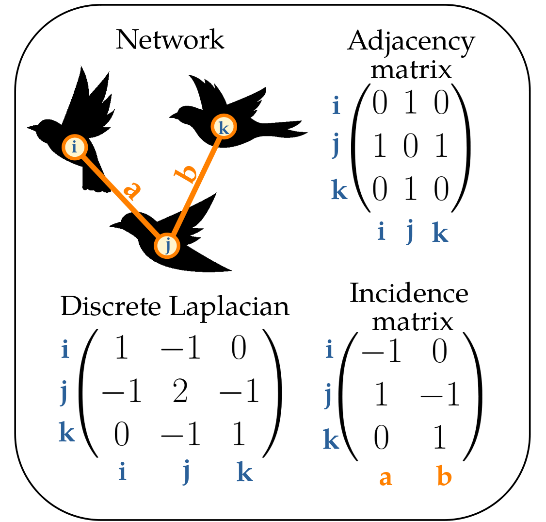
Figure 1: Schematic view of the adjacency matrix $n$, incidence matrix $D$, and discrete Laplacian $\Lambda$ in a very simple network.

II.3.2 From noise on the sites to noise on the links

To produce a noise $\boldsymbol{\xi}_{i}$ whose correlator is proportional to $\Lambda_{ij}$, we can use the discrete Laplacian thermostat introduced in Cavagna et al. (2023b) and further developed in Cavagna et al. (2023c): we must pass from a noise defined on the sites to a noise defined on the links. Let us label the sites of the lattice with $\{i,j,\dots\}$ and the links with $\{a,b,\dots\}$. The incidence matrix, $D_{ia}$, is constructed as follows Gross et al. (2018): after arbitrarily assigning a direction to each link $a$, we set $D_{ia}=+1$ if $i$ is at the end of $a$, $D_{ia}=-1$ if $i$ is at the origin of $a$, and $D_{ia}=0$ if site $i$ does not belong to $a$ (Fig.1); note that, by construction, we have,

$$\sum_{\mathrm{sites\ }i}D_{ia}=0\ .$$ (18)

Notice also that the arbitrariness in the definition of $D_{ia}$ due to the arbitrary choice of the directions of the links, reflects the inevitable arbitrariness in the definition of the derivative on a general discrete lattice. The crucial property of the incidence matrix is that its square over the links is equal to the discrete Laplacian Gross et al. (2018),

$$\sum_{\mathrm{links\ }a}D_{ia}D^{\mathrm{T}}_{aj}=\Lambda_{ij}\ .$$ (19)

If we define on each link $a$ a $\delta$-correlated Gaussian noise, $\boldsymbol{\epsilon}_{a}$, with variance,

$$\langle{\epsilon}^{\mu}_{a}(t){\epsilon}^{\nu}_{b}(t^{\prime})\rangle=2T\,\lambda\;\delta_{ab}\,\delta_{\mu\nu}\,\delta(t-t^{\prime})\ ,$$ (20)

we can now build the site noise acting on each spin $i$ as,

$$\boldsymbol{\xi}_{i}(t)=\sum_{a}D_{ia}\,\boldsymbol{\epsilon}_{a}(t)\ ,$$ (21)

whose variance is,

$$\langle{\xi}^{\mu}_{i}(t){\xi}^{\nu}_{j}(t^{\prime})\rangle = \sum_{ab}D_{ia}D_{jb}\,\langle\epsilon^{\mu}_{a}(t)\epsilon^{\nu}_{b}(t^{\prime})\rangle$$ (22)

$$= \sum_{a}D_{ia}D^{\mathrm{T}}_{aj}\,2T\;\lambda\,\delta_{\mu\nu}\,\delta(t-t^{\prime})$$

$$= 2T\;\lambda\,\Lambda_{ij}\,\delta_{\mu\nu}\,\delta(t-t^{\prime})\ ,$$

so that we recover exactly the desired expression, equation (16). Because by construction $\sum_{i}D_{ia}=0$, from (21) we have that,

$$\sum_{i}\boldsymbol{\xi}_{i}=0\ ,$$ (23)

which makes it even more apparent the fact that the new noise conserves the total spin in (15).

II.3.3 The new model

To summarize, the new fully conservative ISM model is defined by the equations,

$$\begin{split}\frac{d\boldsymbol{r}_{i}}{dt}&=\boldsymbol{v}_{i}\\ \frac{d\boldsymbol{v}_{i}}{dt}&=\frac{1}{\chi}\boldsymbol{s}_{i}\times\boldsymbol{v}_{i}\\ \frac{d\boldsymbol{s}_{i}}{dt}&=\boldsymbol{v}_{i}\times J\sum_{j}n_{ij}\boldsymbol{v}_{j}-\frac{\lambda}{\chi}\sum_{j}\Lambda_{ij}\boldsymbol{s}_{j}+\boldsymbol{\xi}_{i}\ ,\end{split}$$ (24)

where the noise is built from equations (20) and (21), and therefore satisfies,

$$\langle\xi_{i}^{\mu}(t)\xi_{j}^{\nu}(t^{\prime})\rangle=2\lambda\Lambda_{ij}T\delta(t-t^{\prime})\delta_{\mu\nu}.$$ (25)

To distinguish this modified version from the standard ISM, we refer to it as the Fully Conserved Inertial Spin Model (FC-ISM). As previously anticipated, the new Laplacian terms violate the condition $\boldsymbol{s}_{i}\cdot\boldsymbol{v}_{i}=0$, which we therefore decided to relax. The stochastic dynamics anyway keeps it true on average.

We notice that the fact of having introduced a conservative fluctuation-dissipation part, does not prevent us from adding also a dissipative part to the dynamics,

$$\frac{d\boldsymbol{r}_{i}}{dt} =\boldsymbol{v}_{i},$$ (26a)

$$\frac{d\boldsymbol{v}_{i}}{dt} =\frac{1}{\chi}\boldsymbol{s}_{i}\times\boldsymbol{v}_{i},$$ (26b)

$$\frac{d\boldsymbol{s}_{i}}{dt} =\boldsymbol{v}_{i}\times J\sum_{j}n_{ij}\boldsymbol{v}_{j}-\frac{1}{\chi}\sum_{j}(\eta\,\delta_{ij}+\lambda\,\Lambda_{ij})\boldsymbol{s}_{j}+\boldsymbol{\xi}_{i},$$ (26c)

with the corresponding noise,

$$\langle\xi_{i}^{\mu}(t)\xi_{j}^{\nu}(t^{\prime})\rangle=2(\eta\,\delta_{ij}+\lambda\,\Lambda_{ij})\,T\delta(t-t^{\prime})\delta_{\mu\nu}.$$ (27)

We will not study such general model here, but it is important to understand that in principle and in practice, one could; we cannot exclude that a certain amount of bona fide dissipation of the spin is present in natural systems, due to the interaction between the agents and the environment, so the possibility to have both $\eta$ and $\lambda$ in the model gives it more realism and flexibility.

Of course, if we want the model to stay in the underdamped regime we need to keep $\eta$ small enough, and this brings us to the second and most profound reason why having both the dissipative and the non-dissipative irreversible terms is very helpful. When we say that for “small enough” dissipation $\eta$ the system is in the vicinity of the underdamped fixed point, we are not being very specific. Even when we stated that this happens if $L\ll{\cal R}_{c}$, where ${\cal R}_{c}$ is the crossover length scale, we did not give much insight on how this length scale emerges. Once we write (26), however, we can be a bit more specific.

The discrete Laplacian is dimensionless, so out of dimensional consistency we can write, $\Lambda_{ij}\sim-a^{2}\nabla^{2}$, where $a$ is some microscopic length-scale (it would be the lattice spacing, in the equilibrium case). From mere dimensional analysis, then, we see that the ratio $a^{2}\lambda/\eta$ has the dimensions of a square length; moreover, we see that such length-scale diverges for $\eta\to 0$, as we expect from the crossover length scale: if no dissipation is present, the system is underdamped over all scales. It is no surprise then to discover that at the bare level, i.e. without taking into account RG corrections, the crossover length-scale is indeed proportional to,

$${\cal R}^{\mathrm{(bare)}}_{c}\sim\sqrt{\frac{\lambda}{\eta}}\ .$$ (28)

There are RG corrections to this formula, both in the amplitudes (to restore dimensions) and in the exponent Cavagna et al. (2023a), but it is nevertheless very important to keep (28) in mind to give flesh to the statement that the finite-size scale of the microscopic model is underdamped as long as dissipation is small enough.

III Results

To delve into the exploration of the novel fully conservative model, we conduct numerical analyses of equations (24) in both the Fixed Network (FN) and Self-Propelled Particles (SPP) scenarios. We begin by examining the FN case. We simulate the model on a fixed lattice, i.e. without self-propulsion: particles sit on a lattice and the equation $d\boldsymbol{r}_{i}/dt=\boldsymbol{v}_{i}$ is ignored, so that $\boldsymbol{v}_{i}$ is just an orientational degree of freedom not related to the velocity. In this case the model is in the universality class of Halperin and Hohenberg’s Model G Hohenberg and Halperin (1977), a class that also includes the microscopic quantum antiferromagnet. We therefore have clear expectations regarding both the near-critical and the low-temperature phase: in the former, we know the exact values of the critical exponents, while in the latter we anticipate the linear propagation of information in the form of spin waves. This is a good starting point to test the model, since Model G is well-known, and we know what to expect. Once the static equilibrium case has been characterized, we will reintroduce the self-propulsion in the dynamics, $\dot{\boldsymbol{r}}_{i}=\boldsymbol{v}_{i}$. As self-propelled particles move, the underlying interaction network undergoes constant reshuffling. In this scenario, the model falls in the universality class of self-propelled Model G Cavagna et al. (2023a), for which we have clear RG predictions in the near-ordering phase. While we lack a theoretical prediction for the low-temperature case, observations from starling flocks and from previous numerical simulations suggest that we will continue to observe a linear propagation of information.

III.0.1 Numerical details

We have employed a 4th-order Runge-Kutta (RK) method to integrate equations (24). We have chosen this method to ensure that the cross product strictly preserves the norm of $\boldsymbol{v}_{i}$. As mentioned before, we set $|\boldsymbol{v}_{i}|=1$. The time step has been chosen to be $\Delta t=5\times 10^{-4}$, which ensures that all simulations realized for this work converge.

For the FN case, the simulations have been conducted on a cubic lattice of size $L$. The total number of particles/sites is $N=L^{3}$, being then that the inter-particle distance (or lattice step) is $1$. Each site has $n_{c}=2d=6$ neighbours, where Periodic Boundary Conditions (PBC) have been enforced. We have simulated system sizes that span from $L=4$ to $L=18$, with a number of samples depending of $L$.

For the SPP case, the simulations have been conducted on a cubic box of size $L$ (also with PBC). The total number of particles/agents is $N$, while $N$ and $L$ have been chosen to have a density $\rho=\frac{N}{L^{3}}=1$ for all cases. We have simulated system sizes that span from from $L=4$ to $L=14$, with a number of samples depending of $L$. The agents interact by following a metric rule: two agents $i$ and $j$ interact if they are separated by less than a given distance $r_{c}$. In terms of the adjacency matrix $n_{ij}$, this reads

$$\begin{cases}n_{ij}=1\text{ }\text{if }r_{ij}\leq r_{c}\\ n_{ij}=0\text{ }\text{if }r_{ij}>r_{c}.\end{cases}$$ (29)

We take $r_{c}=1.6$, which gives an average number of neighbours around $\sim 17$, as in Cavagna et al. (2023a), since a higher number of neighbours helps to reduce density fluctuations. A larger relaxational coefficient, $\lambda$, also has an important role in controlling density fluctuations. In Cavagna et al. (2023a) - where only standard dissipation was considered - it was not possible to increase the dissipation coefficient $\eta$ to do that, as it would have resulted in being on the wrong side of the RG crossover. For this reason, in that work the social force in Eq. (5) was normalized by the number of interacting neighbours, a procedure that is known to help maintain density homogeneity throughout space and time. Here, on the other hand, we can safely increase the value of $\lambda$ to regularize density without the need of any normalization of the social force.

For both cases, FN and SPP, the parameters have been set to $J=1$ and $\chi=1$, and with $\lambda$ and $T$ values specified for each result. We have carefully tested that all samples reach a stable steady state (i.e. thermalize in the FN case). The initial velocity has been randomly chosen, ensuring that $|\boldsymbol{v}_{i}|=1$. The spins have been initialized as $\boldsymbol{s}_{i}=0,\forall i$. For the SPP case, the initial positions $\boldsymbol{r}_{i}$ have been chosen to be the sites of a cubic lattice.

For both cases (FN and SPP), we have computed the order parameter

$$\Phi=\frac{1}{N}\left\lvert\sum_{i}\frac{\boldsymbol{v}_{i}}{\lvert\boldsymbol{v}_{i}\rvert}\right\rvert,$$ (30)

that allows us to characterize the static phase diagram (Figure 2), and thus to identify the temperature regime where the system is in the ordered and disordered phases, separated by the critical temperature $T_{c}$.

We have also computed the dynamic connected correlation function of the velocities,

$$\leavevmode\resizebox{399.2946pt}{}{$C(\boldsymbol{k},t)=\frac{1}{N}\left\langle\sum_{i,j}^{N}\delta\boldsymbol{v}_{i}(t_{0})\cdot\delta\boldsymbol{v}_{j}(t_{0}+t)e^{-i\boldsymbol{k}\cdot\boldsymbol{r}_{ij}}\right\rangle_{t_{0}}$},$$ (31)

where $\delta\boldsymbol{v}_{i}(t)=\boldsymbol{v}_{i}(t)-(1/N)\sum_{k}\boldsymbol{v}_{k}$ , $\boldsymbol{r}_{ij}=\boldsymbol{r}_{i}(t_{0})-\boldsymbol{r}_{j}(t_{0}+t)$ and $\langle\cdot\rangle_{t_{0}}$ represents an average over the time origin $t_{0}$. To improve statistics we have assumed that the system is isotropic with respect to the direction of $\boldsymbol{k}$, and we have combined the correlation functions of three orthogonal wave-vectors,

$$C(k,t)=\frac{1}{3}\left(C(\boldsymbol{k}_{x},t)+C(\boldsymbol{k}_{y},t)+C(\boldsymbol{k}_{z},t)\right),$$ (32)

where $\boldsymbol{k}_{x}=(k,0,0)$, $\boldsymbol{k}_{y}=(0,k,0)$ and $\boldsymbol{k}_{z}=(0,0,k)$. We have finally computed the correlation function $C(k,\omega)$, defined as the temporal Fourier transform of the correlation function $C(k,t)$.

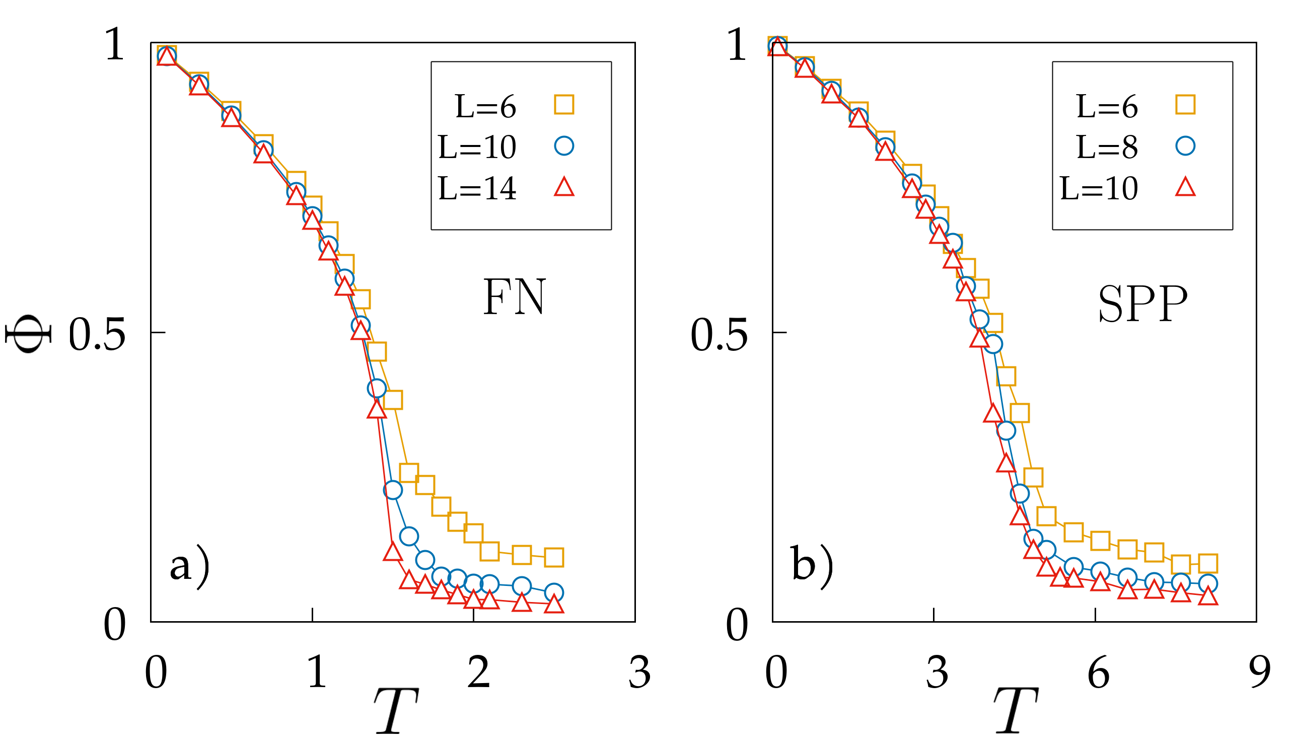
Figure 2: Stationary order parameter $\Phi$ when the temperature $T$ is tuned for different system sizes for a) the FN case (with $\lambda=0.5$) and b) the SPP case (with $\lambda=10$).

III.1 Fixed-Network test of the new model

III.1.1 FN – Near-ordering phase

Classic RG studies of the dynamic critical exponent of Model G give $z=1.5$ Hohenberg and Halperin (1977), a value in full agreement with experiments on perovskites as RbMnF₃ Tucciarone et al. (1971) and with numerical simulations of the Heisenberg antiferromagnet Landau and Krech (1999); Nandi and Täuber (2019); Cavagna et al. (2023b). Here we verify that the fully conserved ISM in the Fixed Network case falls in the same universality class. Calculating the critical exponent $z$ requires using dynamic scaling, where the relaxation time at wavevector $k$ is expressed as

$$\tau_{k}=k^{-z}g(k\xi).$$ (33)

where $g$ is a scaling function and all the dependence on the temperature $T$ goes into the correlation length $\xi$. We can obtain the characteristic correlation time $\tau_{k}$ from the dynamic correlation functions, either in the time domain or in the frequency domain. Following the standard definition in Halperin and Hohenberg (1969), the characteristic frequency $\omega_{k}$ can be calculated from the following relation,

$$\int_{-\omega_{k}}^{\omega_{k}}\frac{d\omega}{2\pi}\frac{C(k,\omega)}{C_{0}(k)}=\frac{1}{2}.$$ (34)

The characteristic frequency $\omega_{k}$ is naturally the inverse of the relaxation time $\tau_{k}$, which – translating (34) in the time domain – is given by,

$$\int_{0}^{\infty}\!\!\frac{dt}{t}\,\frac{C(k,t)}{C(k,t=0)}\sin\left(\frac{t}{\tau_{k}}\right)=\frac{\pi}{4}.$$ (35)

In order to exploit Eq. (33) and to compute the dynamic exponent, it is convenient to identify first the critical regime. From the static correlation function $C(k)=C(k,t=0)$ we obtain the susceptibility $\chi=C(k_{\text{max}})$, where $k_{\text{max}}$ is the wave-vector of the first maximum of $C(k)$. For any given size $L$, we can then identify the finite-size critical temperature $T_{c}(L)$, as the temperature where the susceptibility is maximal. This temperature defines the critical region, where the correlation length is proportional to the system size, i.e. $\xi(T_{c}(L))\sim L$. Working in this regime, we can consider Eq. (33) and choose $k=1/\xi\sim 1/L$. We then get the collective relaxation time of the system as

$$\tau\sim L^{z}.$$ (36)

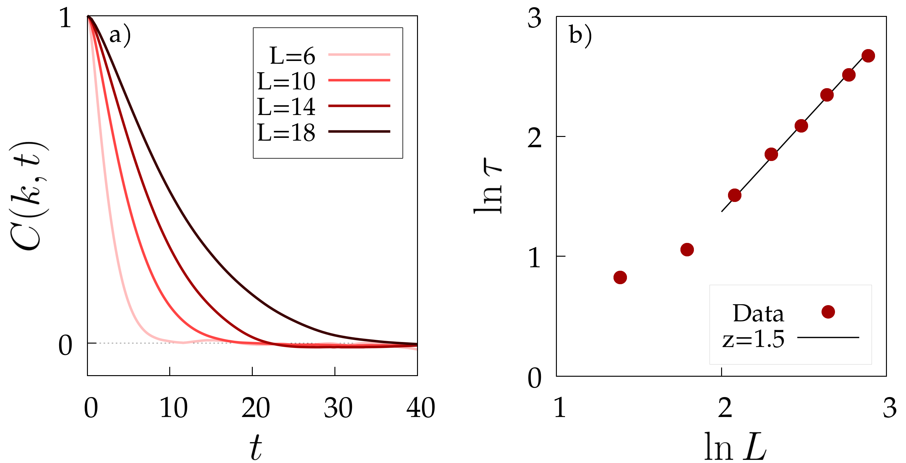
Figure 3: Fixed-network – near ordering: a) Correlation functions $C(k,t)$ as a function of time, at the pseudo-critical temperature $T_{c}(L)$ for different sizes $L$, and $\lambda=0.5$. The correlation functions are normalized by their value in $t=0$, and they are evaluated at $k=2\pi/L$ (see main text). b) Relaxation time $\tau$ as a function of the system’s size $L$. The line indicates the fit with the exact dynamical critical exponent, $z=1.5$, over the six largest sizes.

Eq. (36) provides a straightforward method to compare our simulations with the theoretical prediction of Model G, where $z=1.5$. In Figure 3a) we display several $C(k,t)$ curves, normalized by their value at $t=0$, obtained at the critical temperature for different system sizes. For each one of these curves, we then compute the global relaxation time following Eq. (35), and plot it as a function of $L$. A fit of these data gives us the numerical estimate of the dynamical critical exponent $z$. The result is displayed in panel b) of Figure 3, and it matches quite well the $z=1.5$ value. For thoroughness, we also performed a fitting procedure with a free exponent $z_{\text{fit}}$ using the six largest sizes, yielding $z_{\text{fit}}=1.48\pm 0.04$. Our results therefore confirm that the universality class of the fully conserved ISM in the fixed network (i.e. equilibrium) case is the same as that of the microscopic quantum antiferromagnet, namely the universality class of Model G.

III.1.2 FN – Ordered phase

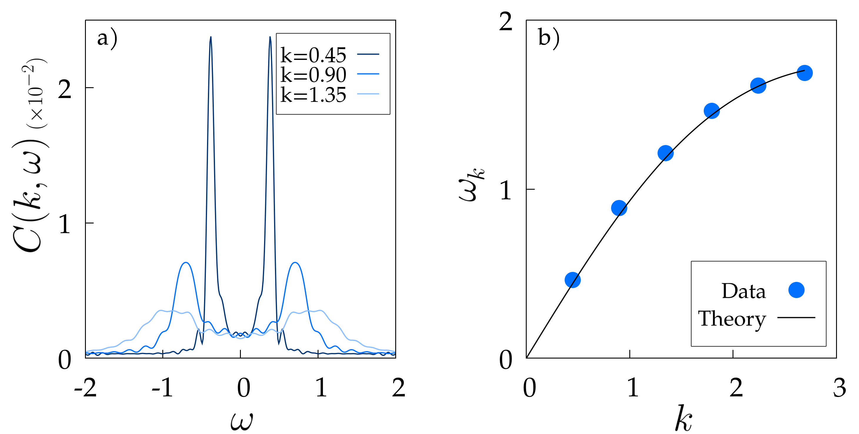
Figure 4: Fixed network – ordered phase: a) Correlation functions $C(k,\omega)$ for different wave-vectors $k$ for a system of size $L=14$ with $T=0.2$ and $\lambda=0.5$. b) Characteristic frequency $\omega_{k}$ computed from Eq. (34) for different values of $k$ (blue points). The continuous curve corresponds to the characteristic frequency of the spin-waves $\omega_{c}(k)$ derived analytically, see Eq. (41).

At low temperatures ($T\ll T_{c}$), the system exhibits spontaneous symmetry breaking. In this regime, Model G exhibits linear propagation of information in the form of spin waves. This characteristic behavior has been verified for the microscopic quantum antiferromagnet Landau and Krech (1999); Cavagna et al. (2023b). In the next paragraphs, we analyze and discuss information propagation and the spin-wave behaviour within the context of the fixed-network FC-ISM.

We note that, due to symmetry breaking, all velocities $\boldsymbol{v}_{i}$ predominantly point in the same mean direction $\boldsymbol{V}=(1/N)\sum_{i}\boldsymbol{v}_{i}$. It is then convenient to rewrite the individual velocities in terms of fluctuations: $\boldsymbol{v}_{i}=\boldsymbol{V}+\delta\boldsymbol{v}_{i}^{L}+\boldsymbol{\pi}_{i}$, where $\boldsymbol{\pi}_{i}\cdot\boldsymbol{V}=0$ and - at low temperature - $|\boldsymbol{\pi}_{i}|\ll|\boldsymbol{V}|$ and $|\delta\boldsymbol{v}_{i}^{L}|\sim O(|\boldsymbol{\pi}_{i}|^{2})$. By rewriting the equations of motion in terms of the variables $\{\boldsymbol{\pi}_{i}\}$ and assuming that $\boldsymbol{V}$ is constant in time, we can expand up to first order, obtaining a linear dynamics for $\boldsymbol{\pi}_{i}$. This procedure is known as the spin-wave expansion. The resulting equation reads

$$\frac{d^{2}\boldsymbol{\pi}_{i}}{dt^{2}}=-\frac{J}{\chi}\sum_{j}\Lambda_{ij}\boldsymbol{\pi}_{j}-\frac{\lambda}{\chi}\sum_{j}\Lambda_{ij}\frac{d\boldsymbol{\pi}_{j}}{dt}+\boldsymbol{\hat{n}}\times\boldsymbol{\xi}_{i},$$ (37)

where $\boldsymbol{\hat{n}}$ is the collective direction of motion. In the continuum limit, when $\Lambda_{ij}\to-\nabla^{2}$, the propagator (Green function) of the homogeneous differential equation can be easily computed in Fourier space giving the following dispersion relation for its poles,

$$\tilde{\omega}(k)=-\frac{\lambda k^{2}}{2\chi}i\pm\sqrt{\frac{Jk^{2}}{\chi}-\left(\frac{\lambda k^{2}}{2\chi}\right)^{2}}.$$ (38)

The imaginary part of $\tilde{\omega}$ encodes the decay in time of the $C(k,t)$. The real part of $\tilde{\omega}$, that we denote here as $\omega_{c}$, represents the characteristic frequency of oscillation of the correlation function $C(k,t)$ (or the spin waves frequency). The characteristic frequency $\omega_{c}(k)$ is,

$$\omega_{c}(k)=\sqrt{\frac{Jk^{2}}{\chi}-\left(\frac{\lambda k^{2}}{2\chi}\right)^{2}}.$$ (39)

In fact, however, we work on a discrete cubic lattice with periodic boundary conditions (PBC), for which the eigenvalues of the Laplacian operator are not $k^{2}$ but rather $4\sin^{2}(k/2)$; hence, the actual dispersion relation for our simulation should be,

$$\tilde{\omega}(k)=-\frac{\lambda 4(\sin{\frac{k}{2}})^{2}}{2\chi}i\pm\sqrt{\frac{J4(\sin{\frac{k}{2}})^{2}}{\chi}-\left(\frac{\lambda 4(\sin{\frac{k}{2}})^{2}}{2\chi}\right)^{2}},$$ (40)

and hence,

$$\omega_{c}(k)=\sqrt{\frac{J4(\sin{\frac{k}{2}})^{2}}{\chi}-\left(\frac{\lambda 4(\sin{\frac{k}{2}})^{2}}{2\chi}\right)^{2}}$$ (41)

The most direct way to analyze the characteristic frequency of oscillation in our simulations is by focusing on $C(k,\omega)$. The correlation functions $C(k,\omega)$ obtained from our simulations distinctly reveal the presence of a smooth peak at a specific frequency (see Figure 4 a)). Notably, the position of this peak varies with the value of $k$. To compute numerically the characteristic frequency for different values of $k$, we resort to Eq. (34). Indeed it can be easily shown that, in presence of a dominant mode, $\omega_{k}$ tends to the frequency of that mode Halperin and Hohenberg (1969). In Figure 4 b), we then compare the characteristic frequencies obtained directly from the simulations with the analytical expression $\omega_{c}(k)$ derived from the spin-wave expansion (41). In conclusion, the numerical data confirm the presence of propagating spin waves in the fixed-network fully conserved ISM and they are in full agreement with the theoretical predictions of the spin-wave expansion.

III.2 Self-propelled test of the new model

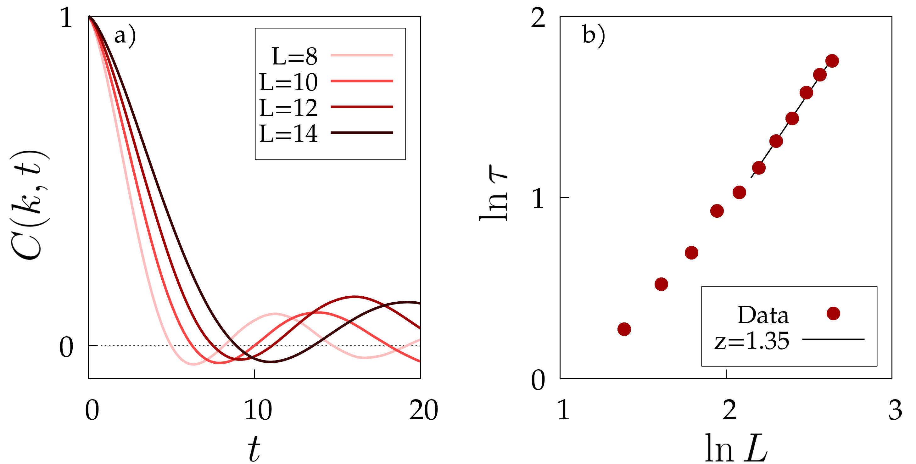
Figure 5: Self-propelled case – near ordering: a) Correlation functions $C(k,t)$ at the pseudo-critical temperature $T_{c}(L)$ for different sizes $L$, and $\lambda=10$. The correlation functions are normalized by their value in $t=0$, and they are evaluated at $k=2\pi/L$. b) Relaxation time $\tau$ as a function of the system’s size $L$. The line indicates the fit with the theoretical dynamical critical exponent, $z=1.35$, over the six largest sizes.

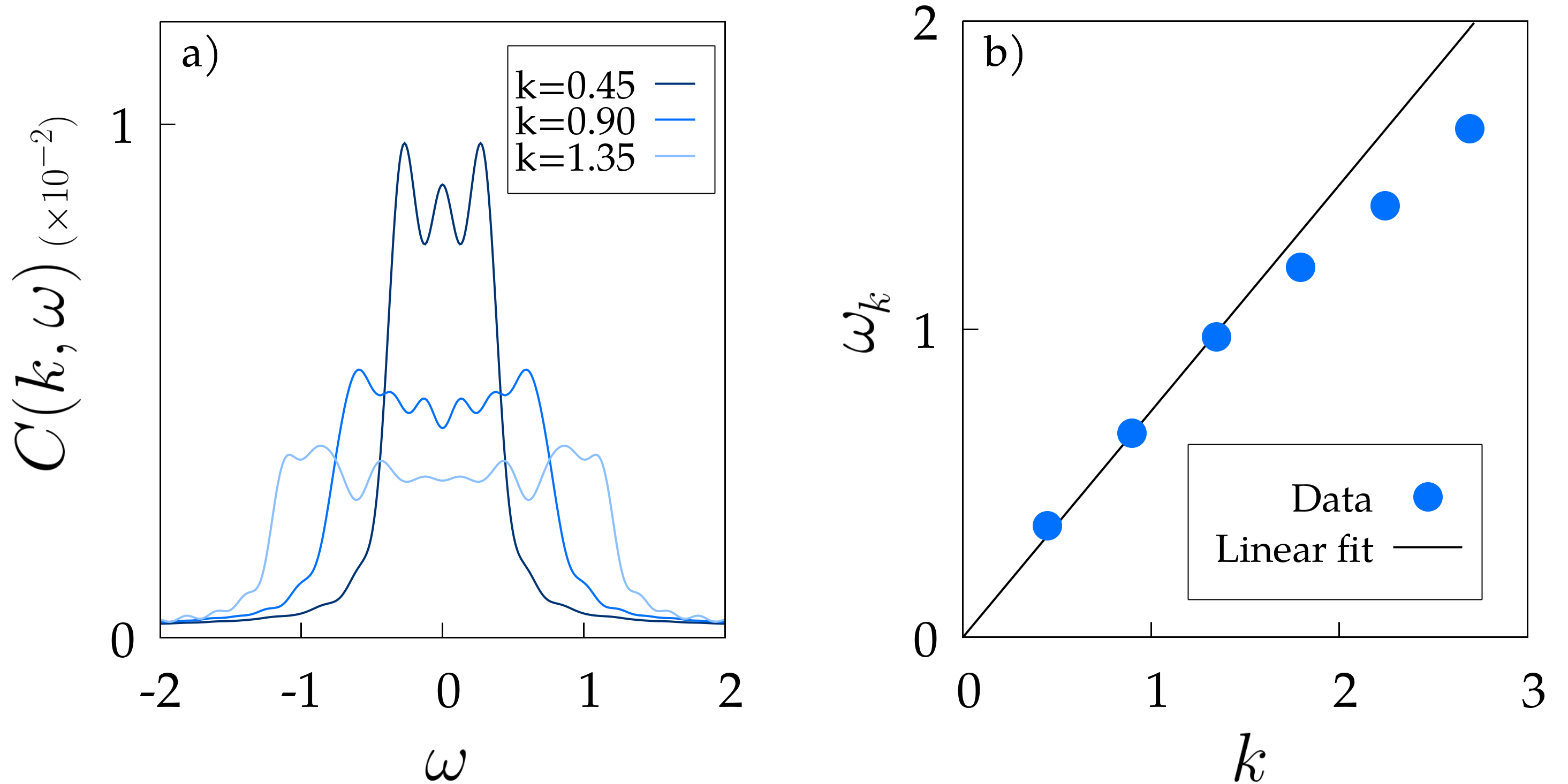
Figure 6: Self-propelled case – ordered phase a) Correlation functions $C(k,\omega)$ for different wave-vectors $k$ for a system of size $L=14$ with $T=0.5$ and $\lambda=10$. b) Characteristic frequency $\omega_{k}$ computed from Eq. (34) for different values of $k$ (blue points); the straight line is a linear fit of the three lowest-$k$ data points.

III.2.1 SPP – Near-ordering phase

The dynamic critical exponent of the self-propelled Model G is known to be $z=1.35$, which is compatible with the estimate of $z$ from experimental data of midge swarms Cavagna et al. (2023a). As also discussed in Cavagna et al. (2023a), numerical simulations of the standard ISM model (i.e., $\lambda=0$), performed with sufficiently small $\eta$, also yield an exponent $z$ consistent with $1.35$. However, as discussed previously, the standard ISM is quite limited if we want to explore the conservative universality class. Indeed, it exhibits this class behaviour only for $L\ll{\cal R}_{c}(\eta)$ so that for larger sizes it requires increasingly smaller values of $\eta$, which in turn requires increasingly longer simulation times. Here, on the other hand, we will determine $z$ in simulations of the purely conservative ISM, where these problems do not arise.

To obtain $z$, we follow the same procedure described in section III.1.1. In Figure 5a) we display the correlation functions $C(k,t)$ at the critical temperature, for several values of $k$. At short times, we can observe the effect of inertia (i.e. a decay that is not exponential), much in the same way as for the fixed network case. After the initial decay, however, there appears to be an oscillation even at the near-ordering temperature, which was not present on the fixed lattice. We currently lack a clear explanation for this phenomenon; this is a non-equilibrium model for which we do not have a full theoretical prediction other than the RG determination of $z$. However, we can put forward an educated guess. In systems with a low-temperature spin wave phase (antiferromagnets and, more generally, the Model G class), it is well known that some precursors of the low-$T$ phase emerge already around the critical temperature Marshall and Harwell (1965). Such precursors (called ”paramagnons” in the cond-mat literature Marshall and Harwell (1965)) show themselves as unexpected real parts of the characteristic frequency, in a phase where one would only expect an imaginary part; hence, in the domain of time, they are simply extra oscillations in the $C(k,t)$. The specific form of paramagnons is known to be highly dependent on the specific details of the material/model under consideration, hence it may very well be that the out-of-equilibrium version of the fully conserved ISM merely has a more pronounced abundance of paramagnons compared to its equilibrium counterpart. A more careful investigation of the numerical data and of the background theory are required to clarify this point; this is left for future research.

In any case, whatever is the specific shape of the $C(k,t)$, we can calculate the largest relaxation time $\tau$ from $C(k,t)$ at the pseudo-critical temperature $T_{c}(L)$ and plot the obtained relaxation times $\tau$ vs. $L$. This is exactly what we show in panel b) of Figure 5: our results show that our simulations are in complete agreement with the prediction of the self-propelled Model G, i.e, $z=1.35$. For the sake of completeness, we fit a free exponent to the six largest sizes, obtaining an exponent $z_{fit}=1.36\pm 0.04$. We remark that this is the first determination of the exponent $z$ from simulations falling in the universality class of self-propelled Model G without the need to exploit a finite-size crossover, nor (which is the same) the need to tune any specific parameter (i.e. the friction $\eta$, as it occurs in the standard ISM).

III.2.2 SPP – Ordered phase

As in the FN case, the system undergoes spontaneous symmetry breaking in the low temperature regime ($T\ll T_{c}$). This manifests as a collective alignment of the individual velocities, with most of the particles moving coordinately along the polarization direction. From a biological standpoint, this behaviour mirrors the coordinated motion observed in starling flocks. We notice at this point a difference between our study of the FC-ISM up to now and the real dynamics of starling flocks. Previous studies have highlighted the topological nature of interactions within natural flocks Ballerini et al. (2008), where individuals interact with their $n_{c}$ nearest neighbours, rather than with all individuals within a fixed radius $r_{c}$ (metric interaction), which is what we have implemented thus far into the FC-ISM. The problem is that topological interactions can be non-reciprocal: the fact that one bird interacts with another does not imply that the second bird interacts back with the first ($n_{ij}\neq n_{ji}$). Within the present definition of the fully-conservative model, this fact can potentially violate the conservation law of the spin. Therefore, we opt to retain metric-based interactions here, prioritizing the exploration of conservation law effects over an exact replication of starling flock behaviour. We leave the (perhaps non-trivial) generalization of the fully conservative model to non-reciprocal interactions to future work.

The procedure we follow to characterize information propagation is the same adopted in Section III.1.2 for the fixed network model. In contrast with the equilibrium case, though, there is no analytical determination, nor any previous theoretical study of the dispersion relation in the active ISM to compare our data with. Yet, we do expect the presence of linearly propagating modes, at least in the low $k$ limit. Indeed, this is what has been observed in experiments on natural starling flocks Attanasi et al. (2014a), which led to development of the ISM in the first place. Besides, numerical simulations of the dissipative ISM, in its low $\eta$ regime, confirm the existence of linearly propagating modes in the system. Moreover, from a theoretical point of view, the fact that the fixed-network counterpart has linearly propagating modes, together with the observation that in the deeply ordered phase the interaction network $n_{ij}(t)$ changes very slowly in time Mora et al. (2016), suggests that linear propagating modes of the orientation should survive also in the active regime. Yet, of course, we have no reason to expect that the full dispersion relation in the active case is exactly the same as in the equilibrium one.

In Figure 6 a), we show the correlation functions $C(k,\omega)$ of the active, fully conservative ISM. The first thing we notice is that the structure of the peaks is significantly more complicated than in the equilibrium case, Fig.4; hence – as anticipated above – the dispersion relation of the active model is different from that of the equilibrium case. Apart from statistical effects (the need of averaging over many more samples) and the obvious effect of activity, namely the (slow) reshuffling of the interaction network $n_{ij}(t)$, there might be another underlying reason for the rather complicated shape of $C(k,\omega)$ that we find. In the present analysis of the numerical data, and in particular in our definition of the correlation function, we are assuming isotropy; while this is certainly true in the near-ordering phase, it is far less trivial an hypothesis in the low temperature phase, in which rotational symmetry is spontaneously broken. The fact that the equilibrium theory does not display an anisotropic structure of the correlation functions even in the symmetry-broken phase is quite an accident of equilibrium, which needs not be inherited by the out-of-equilibrium active model (for example, anisotropic correlation functions are theoretically expected and observed in the ordered phase of the Vicsek model Tu et al. (1998b)). If this is the case, namely if some anisotropic structure is present in the active correlations, then by averaging in an isotropic way we are possibly creating a complicated structure by mixing qualitatively different propagating modes. The detailed study of a possible anisotropic structure requires much heavier numerical simulations and it is left to further studies. This notwithstanding, we may still ask whether the mean characteristic frequency, defined with the half-width method, has a linear dependence on $k$ or not. The answer to this question is positive: Figure 6) b) reveals a linear correlation between the frequency $\omega_{k}$ and $k$ at small momentum, consistently with previous simulations on the dissipative ISM and with the experimental data on starling flocks. Even though – as we said – a more detailed study of the low-temperature phase is certainly needed to fully explore the dispersion relation, these results confirm that the spin conservation law is responsible for creating linearly propagating modes of the orientation in the active ordered phase of SPP models.

IV Conclusions

We have presented and tested numerically a version of the inertial spin model with relaxational terms (dissipation and noise), but where the total spin is nevertheless strictly conserved. The formalism we have used exploits the recently introduced discrete Laplacian thermostat of Cavagna et al. (2023b, c). The framework also allows for additional non-conserving spin dissipation (see Eq. (26)), but we have not tested this more general case in simulations. The main motivation for the introduction of this model is that it provides a microscopic model belonging to the dynamic universality class of active, inertial and conservative systems, corresponding to the new RG fixed point recently described in the inertial active field theory of Ref. Cavagna et al. (2023a). The original dissipative ISM, in contrast, is described by this fixed point only at sufficiently low dissipation and sufficiently small system size, being ruled in the thermodynamic limit by an overdamped fixed point. As we have pointed out, the strict thermodynamic limit is of little use to describe biological groups, which are rather small and can thus be ruled by unstable fixed points in the presence of crossover phenomena. Nevertheless, it is theoretically desirable to be able to pinpoint at least one microscopic model that is strictly (i.e. in the thermodynamic limit) a member of this new universality class.

We have considered first the fixed-lattice (non-active) version of the model. Since this equilibrium case should belong to the well-known class of Model G, it serves as a test for the model and for the numerical procedure. In the near-critical region we have found the dynamical critical exponent to be fully compatible with $z=1.5$ (the exponent is known to be exactly $z=3/2$ in this case Hohenberg and Halperin (1977)). In the low-temperature phase, the dynamic correlation function $C(k,\omega)$ shows clear spin-wave peaks and the observed dispersion relation coincides with the theoretical result.

We then simulated the active (self-propelled) model, which is of course out-of-equilibrium. In this case, the available theoretical results are limited. In the near-critical regime, we found $z=1.35$, which coincides with the one-loop RG result as well as with the numerical simulations of the weakly dissipative ISM Cavagna et al. (2023a); incidentally, this is also the exponent measured in experiments on natural swarms of midges. The simulations in the near-ordering region show that this model is less prone to developing density heterogeneities. Density fluctuations, and their coupling to the order parameter, are the reason why the ordering transition in the Vicsek model is discontinuous in the thermodynamic limit Ramaswamy (2010); Toner (2012); Ihle (2011); Solon et al. (2015); Chaté (2020). However, finite-size effects are strong, and the phenomenology of continuous transitions is observed in not-too-large systems both in simulations Chaté et al. (2008) and in actual biological groups Attanasi et al. (2014b). To study this phenomenology theoretically, incompressibility is added as a hard constraint (as e.g. in Chen et al. (2015); Cavagna et al. (2023a)). In numerical studies, the size at which the discontinuous phenomenology starts to be observed depends strongly on the details of the model (such as discrete vs. continuous time Chepizhko et al. (2021) or scalar vs. vector noise Chaté et al. (2008)). To study the critical regime of the (dissipative) ISM, the simulations of Ref. Cavagna et al. (2023a) normalized the alignment coupling $J$ by the number of particles within the interaction radius, $J\to J/\sum_{i}n_{ij}$, a prescription that is known to make the model less prone to phase separation Chepizhko et al. (2021), to avoid spatial density fluctuations. In this work we have not used such normalization; it turns out that the fully-conserved ISM is less prone to such fluctuations (at similar system sizes), simply because we can increase the amount of stochasticity by increasing the relaxational coefficient $\lambda$, with no fear of dissipating the spin.

We have also looked for spin waves in the ordered phase of the active model. There are no theoretical results to look at for guidance in this case, but the expectation from experimental results in flocks Attanasi et al. (2014a), and simulations on the weakly dissipative ISM Cavagna et al. (2015), is that there should be propagating modes with a linear dispersion relation (second sound). We have found excitations showing up as peaks in $C(k,\omega)$ that, although somewhat broad, do display a dispersion relation with a linear real part. However, the phenomenology of the low temperature phase clearly needs further investigation; in particular, the question of a possible anisotropic structure of the correlation functions should be addressed.

Another question that remains open is the following: the ordered phase of ISM is a good candidate to describe flocks of birds; however, it is known that in starling flocks interactions are topological rather than metric Ballerini et al. (2008). It is not clear how to deal with topological interactions in this model. Topological interactions lead to a non-symmetric adjacency matrix (because particle $i$ being $n$-th nearest neighbour of particle $j$ does not necessarily imply the reciprocal relation), thus violating strict spin conservation at the deterministic level. One could still introduce spin-conserving noise (employing a different matrix for the dissipative part), but it is not clear how this would mix with a non-conserving deterministic interaction, and what difference would it make with respect to the dissipative case. The topological case calls for a detailed separate study.

Despite the several open questions, this first test of the new conservative model shows that it can be useful for numerical studies of the active, inertial and conservative universality class, with no possible complications due to the presence of the small dissipation, as in the original ISM. An important instance in which the complete absence of dissipation may help in the analysis is the following. As we repeatedly remarked, the very complicated structure of spin-wave excitations in the low temperature phase of the active model has yet to be fully understood. However, by construction, it is clear that this complicated structure cannot be due to the presence of dissipation, as one could have surmised if the original dissipative ISM had been used to simulate the system. Although this and other issues remain open to further studies, the usefulness of the present model seems promising.

References

- Vicsek et al. (1995) T. Vicsek, A. Czirók, E. Ben-Jacob, I. Cohen, and O. Shochet, Phys. Rev. Lett. 75, 1226 (1995).
- Reynolds (1987) C. W. Reynolds, in Proceedings of the 14th annual conference on Computer graphics and interactive techniques (1987) pp. 25–34.
- Toner and Tu (1995) J. Toner and Y. Tu, Phys. Rev. Lett. 75, 4326 (1995).
- Ramaswamy (2010) S. Ramaswamy, Annual Review of Condensed Matter Physics 1, 323 (2010).
- Ginelli (2016) F. Ginelli, The European Physical Journal Special Topics 225, 2099 (2016).
- Chaté (2020) H. Chaté, Annu Rev Condes Matter Phys. 11, 189 (2020).
- Tu et al. (1998a) Y. Tu, J. Toner, and M. Ulm, Phys. Rev. Lett. 80, 4819 (1998a).
- Grégoire and Chaté (2004) G. Grégoire and H. Chaté, Physical review letters 92, 025702 (2004).
- Chaté et al. (2008) H. Chaté, F. Ginelli, G. Grégoire, and F. Raynaud, Phys. Rev. E 77, 046113 (2008).
- Chaté et al. (2008) H. Chaté, F. Ginelli, G. Grégoire, F. Peruani, and F. Raynaud, Eur. Phys. J. B 64, 451 (2008).
- Moreno et al. (2020) J. C. Moreno, M. L. Rubio Puzzo, and W. Paul, Phys. Rev. E 102, 022307 (2020).
- Chepizhko et al. (2021) O. Chepizhko, D. Saintillan, and F. Peruani, Soft Matter 17, 3113 (2021).
- Attanasi et al. (2014a) A. Attanasi, A. Cavagna, L. Del Castello, I. Giardina, T. S. Grigera, A. Jelić, S. Melillo, L. Parisi, O. Pohl, E. Shen, and M. Viale, Nature Physics 10, 691 (2014a).
- Cavagna et al. (2015) A. Cavagna, L. Del Castello, I. Giardina, T. Grigera, A. Jelic, S. Melillo, T. Mora, L. Parisi, E. Silvestri, M. Viale, et al., Journal of Statistical Physics 158, 601 (2015).
- Cavagna et al. (2017) A. Cavagna, D. Conti, C. Creato, L. Del Castello, I. Giardina, T. S. Grigera, S. Melillo, L. Parisi, and M. Viale, Nature Physics 13, 914 (2017).
- Cavagna et al. (2023a) A. Cavagna, L. Di Carlo, I. Giardina, T. S. Grigera, S. Melillo, L. Parisi, G. Pisegna, and M. Scandolo, Nature Physics , 1 (2023a).
- Ha et al. (2019) S.-Y. Ha, D. Kim, D. Kim, and W. Shim, J Nonlinear Sci 29, 1301 (2019).
- Markou (2021) I. Markou, “Invariance of velocity angles and flocking in the Inertial Spin model,” (2021), 2110.14388 [math] .
- Benedetto et al. (2020) D. Benedetto, P. Buttà, and E. Caglioti, Math. Models Methods Appl. Sci. 30, 1987 (2020).
- Ko et al. (2023) D. Ko, S.-Y. Ha, E. Lee, and W. Shim, Stud. Appl. Math. 151, 975 (2023).
- Huh and Kim (2022) H. Huh and D. Kim, Quart. Appl. Math. 80, 53 (2022).
- Cavagna et al. (2018) A. Cavagna, I. Giardina, and T. S. Grigera, Physics Reports 728, 1 (2018).
- Carruitero et al. (2023) S. Carruitero, A. C. Duran, G. Pisegna, M. B. Sturla, and T. S. Grigera, arXiv preprint arXiv:2312.06368 (2023).
- Cavagna et al. (2019a) A. Cavagna, L. Di Carlo, I. Giardina, L. Grandinetti, T. S. Grigera, and G. Pisegna, Phys. Rev. Lett. 123, 268001 (2019a).
- Cavagna et al. (2019b) A. Cavagna, L. Di Carlo, I. Giardina, L. Grandinetti, T. S. Grigera, and G. Pisegna, Phys. Rev. E 100, 062130 (2019b).
- Hohenberg and Halperin (1977) P. C. Hohenberg and B. I. Halperin, Rev. Mod. Phys. 49, 435 (1977).
- Gross et al. (2018) J. L. Gross, J. Yellen, and M. Anderson, Graph theory and its applications (Chapman and Hall/CRC, 2018).
- Cavagna et al. (2023b) A. Cavagna, J. Cristín, I. Giardina, and M. Veca, Physical Review B 107, 224302 (2023b).
- Cavagna et al. (2023c) A. Cavagna, J. Cristín, I. Giardina, and M. Veca, arXiv preprint arXiv:2312.13065 (2023c).
- Tucciarone et al. (1971) A. Tucciarone, H. Lau, L. Corliss, A. Delapalme, and J. Hastings, Physical Review B 4, 3206 (1971).
- Landau and Krech (1999) D. Landau and M. Krech, Journal of Physics: Condensed Matter 11, R179 (1999).
- Nandi and Täuber (2019) R. Nandi and U. C. Täuber, Physical Review B 99, 064417 (2019).
- Halperin and Hohenberg (1969) B. I. Halperin and P. C. Hohenberg, Phys. Rev. 177, 952 (1969).
- Marshall and Harwell (1965) W. Marshall and G. B. Harwell, National Bureau of Standards Miscellaneous Publication , 135 (1965).
- Ballerini et al. (2008) M. Ballerini, N. Cabibbo, R. Candelier, A. Cavagna, E. Cisbani, I. Giardina, V. Lecomte, A. Orlandi, G. Parisi, A. Procaccini, et al., Proc. Natl. Acad. Sci. 105, 1232 (2008).
- Mora et al. (2016) T. Mora, A. M. Walczak, L. Del Castello, F. Ginelli, S. Melillo, L. Parisi, M. Viale, A. Cavagna, and I. Giardina, Nature Physics 12, 1153 (2016).
- Tu et al. (1998b) Y. Tu, J. Toner, and M. Ulm, Phys. Rev. Lett. 80, 4819 (1998b).
- Toner (2012) J. Toner, Phys. Rev. E 86, 031918 (2012).
- Ihle (2011) T. Ihle, Phys. Rev. E 83 (2011), 10.1103/PhysRevE.83.030901.
- Solon et al. (2015) A. P. Solon, H. Chaté, and J. Tailleur, Phys. Rev. Lett. 114, 068101 (2015).
- Attanasi et al. (2014b) A. Attanasi, A. Cavagna, L. Del Castello, I. Giardina, S. Melillo, L. Parisi, O. Pohl, B. Rossaro, E. Shen, E. Silvestri, and M. Viale, Phys. Rev. Lett. 113, 238102 (2014b).
- Chen et al. (2015) L. Chen, J. Toner, and C. F. Lee, New Journal of Physics 17, 042002 (2015).