On Weakly Contracting Dynamics for Convex Optimization

Abstract

We investigate the convergence characteristics of dynamics that are globally weakly and locally strongly contracting. Such dynamics naturally arise in the context of convex optimization problems with a unique minimizer. We show that convergence to the equilibrium is linear-exponential, in the sense that the distance between each solution and the equilibrium is upper bounded by a function that first decreases linearly and then exponentially. As we show, the linear-exponential dependency arises naturally in certain dynamics with saturations. Additionally, we provide a sufficient condition for local input-to-state stability. Finally, we illustrate our results on, and propose a conjecture for, continuous-time dynamical systems solving linear programs.

I Introduction

Problem description and motivation: A paradigm that is becoming popular to analyze possibly time-varying optimization problems (OP) is to synthesize continuous-time dynamical systems that converge to an equilibrium that is also the optimal solution of the problem. A suitable tool to assess convergence is contraction theory [14, 3]. For OPs with strongly convex costs, the corresponding gradient dynamics, primal-dual dynamics (in the presence of constraints), or proximal gradient dynamics (for non-smooth costs) are strongly contracting, implying that trajectories converge to the equilibrium, which is also the optimal solution. In contrast, for OPs with only convex costs, the corresponding gradient, primal-dual, or proximal gradient dynamics are weakly contracting (or nonexpansive), and convergence depends on the existence of the minimizer.

In this context, we focus on convex OPs with a unique minimizer via continuous-time dynamical systems. These OPs lead to continuous-time dynamics that are globally-weakly contracting in the state space and only locally-strongly contracting (GW-LS-C). For such dynamics, we provide a comprehensive analysis, characterizing their convergence properties and local input-to-state stability (ISS). Finally, as an application, we consider linear programming (LP) to illustrate the effectiveness of our results.

Literature review: Studying optimization algorithms as continuous-time dynamical systems has been an active research area since [1], with, e.g., [17] being one of the first works to design neural networks for LPs. A neural network for solving LPs based on non-differentiable penalty functions has been proposed in [5]. Recently, there has been a renewed interest in continuous-time dynamics for optimization thanks to developments of, e.g., online and dynamic feedback optimization [2]. Additionally, OPs have been related to dynamical systems via proximal gradients, and the corresponding continuous-time proximal gradient dynamics are studied in, e.g., [10, 11]. Proximal gradients dynamics and contraction theory have been exploited in [8], [4] for tackling problems with strongly convex and only convex costs, respectively. In a broader context, there has been a growing interest in using strongly contracting dynamics to tackle OPs [15, 8]. This is mainly due to the fact that such dynamics enjoy highly ordered transient and asymptotic behaviors. Specifically, (i) initial conditions are exponentially forgotten and the distance between any two trajectories decays exponentially quickly [14], (ii) unique globally exponential stable equilibrium for time-invariant dynamics [14] (iii) entrainment to periodic inputs [16] (iv) highly robust behavior, such as ISS [18]. The asymptotic behavior of weakly contracting dynamics is instead characterized in, e.g., [7] for monotone systems and in [12] for primal-dynamics with a locally stable equilibrium.

Contributions: We analyze convergence of GW-LS-C dynamics, showing that this is linear-exponential, in the sense that the distance between each solution of the system and the equilibrium is upper bounded by a linear-exponential function, introduced in this paper. Through a novel technical result, we characterize the evolution of certain dynamics with saturation in terms of the linear-exponential function. This technical lemma is exploited for our convergence analysis, which is carried out considering two cases that require distinct mathematical approaches. First, we consider systems that are GW-LS-C with respect to (w.r.t.) the same norm. Then, we consider the case where the dynamics is GW-LS-C w.r.t. two different norms. Specifically, we give a convergence bound that, as discussed below, is sharper than the one in [4]. Additionally, we characterize local ISS for input-dependent dynamics that are GW-LS-C w.r.t. the same norm. Finally, we show the effectiveness of our results by considering a continuous-time dynamics tackling LPs and propose a general conjecture. The code to replicate our numerical example is given at https://shorturl.at/vGNY1.

While the treatment in this paper is inspired by the results in [4], we extend those results in several ways. First, when the dynamics is GW-LS-C w.r.t. two different norms, the bound we give here is continuous and always sharper than one given in [4], see Remark III.7. Second, when the dynamics is GW-LS-C w.r.t. the same norm, the technical lemma used to establish linear-exponential convergence is novel. Third and finally, local ISS was not considered in [4].

II Mathematical Preliminaries

We denote by $\mbox{0}_{n}\in\mathbb{R}^{n}$ the all-zeros vector of size $n$. Vector inequalities of the form $x\leq(\geq)y$ are entrywise. We let $I_{n}$ be the $n\times n$ identity matrix. Given $A,B\in\mathbb{R}^{n\times n}$ symmetric, we write $A\preceq B$ (resp. $A\prec B$) if $B-A$ is positive semidefinite (resp. definite). We denote by $\lambda_{\textup{max}}(A)$ the maximum eigenvalue of $A$. We say that $A$ is Hurwitz if $\alpha(A):=\max\{\operatorname{Re}(\lambda)\;|\;\lambda\text{ eigenvalue of }A\}<0$, where $\operatorname{Re}(\lambda)$ denotes the real part of $\lambda$.

Norms, Logarithmic Norms and Weak Pairings

We let $\|\cdot\|$ denote both a norm on $\mathbb{R}^{n}$ and its corresponding induced matrix norm on $\mathbb{R}^{n\times n}$. Given $x\in\mathbb{R}^{n}$ and $r>0$, we let $B_{p}{\bigl{(}x,r\bigr{)}}:=\{z\in\mathbb{R}^{n}\;|\;\|z-x\|_{p}\leq r\}$ be the ball of radius $r$ centered at $x$ computed with respect to the norm $p$. Given two norms $\|\cdot\|_{\alpha}$ and $\|\cdot\|_{\beta}$ on $\mathbb{R}^{n}$ there exist positive equivalence coefficients $k_{\alpha}^{\beta}$ and $k_{\beta}^{\alpha}$ satisfying $\|x\|_{\alpha}\leq k_{\alpha}^{\beta}\|x\|_{\beta}$, $\|x\|_{\beta}\leq k_{\beta}^{\alpha}\|x\|_{\alpha}$, $\forall x\in\mathbb{R}^{n}$. The equivalence ratio between $\|\cdot\|_{\alpha}$ and $\|\cdot\|_{\beta}$ is $k_{\alpha,\beta}:=k_{\alpha}^{\beta}k_{\beta}^{\alpha}$, with $k_{\alpha}^{\beta}$ and $k_{\beta}^{\alpha}$ minimal equivalence coefficients.

Given $A\in\mathbb{R}^{n\times n}$ the logarithmic norm (log-norm) induced by $\|\cdot\|$ is

$$\mu(A):=\lim_{h\to 0^{+}}\frac{\|I_{n}{+}hA\|-1}{h}.$$

For an $\ell_{p}$ norm, $p\in[1,\infty]$, and for an invertible $Q\in\mathbb{R}^{n\times n}$, the $Q$-weighted $\ell_{p}$ norm is $\|x\|_{p,Q}:=\|Qx\|_{p}$. The corresponding log-norm is $\mu_{p,Q}\bigl{(}A\bigr{)}=\mu_{p}(QAQ^{-1})$.

We let $\left\llbracket{\cdot},{\cdot}\right\rrbracket$ denote a weak pairing on $\mathbb{R}^{n}$ compatible with the norm $\|\cdot\|$. We recall some of the main standing assumption on weak paring useful for our analysis.

Definition 1:

A weak pairing $\left\llbracket{\cdot},{\cdot}\right\rrbracket$, compatible with the norm $\|\cdot\|$, satisfies:

1. sub-additivity of first argument: $\left\llbracket{x+z},{y}\right\rrbracket\leq\left\llbracket{x},{y}\right\rrbracket+\left\llbracket{z},{y}\right\rrbracket$,  for all $x,y,z\in\mathbb{R}^{n}$;

2. curve norm derivative formula: $\|y(t)\|D^{+}\|y(t)\|=\left\llbracket{\dot{y}(t)},{y(t)}\right\rrbracket$, for every differentiable curve $y\colon]a,b[\rightarrow\mathbb{R}^{n}$ and a.e. $t\in]a,b]$;

3. Cauchy-Schwartz inequality: $\left|\left\llbracket{x},{y}\right\rrbracket\right|\leq\|x\|\|y\|$,  for all $x,y\in\mathbb{R}^{n}$;

4. Lumer’s equality: $\displaystyle\mu\bigl{(}A\bigr{)}=\sup_{z\in\mathbb{R}^{n},z\neq\mbox{0}_{n}}\frac{\left\llbracket{Az},{z}\right\rrbracket}{\left\llbracket{z},{z}\right\rrbracket}$, for every $A\in\mathbb{R}^{n\times n}$.

We refer to [3] for a recent review of those tools.

Mathematical Operators

Given two normed spaces $(\mathcal{X},\|\cdot\|_{\mathcal{X}})$, $(\mathcal{Y},\|\cdot\|_{\mathcal{Y}})$, a map $T\colon\mathcal{X}\rightarrow\mathcal{Y}$ is Lipschitz with constant $L\geq 0$ if $\|T(x_{1})-T(x_{2})\|_{\mathcal{Y}}\leq L\|x_{1}-x_{2}\|_{\mathcal{X}}$, for all $x_{1},x_{2}\in\mathcal{X}$. The upper-right Dini derivative of a function $f\colon\mathbb{R}\rightarrow\mathbb{R}$ is $D^{+}f:=\limsup_{h\to 0^{+}}\bigl{(}f(t+h)-f(t)\bigr{)}/h$. The ceiling function, $\lceil\ \rceil\colon\mathbb{R}\rightarrow\mathbb{Z}$, is defined by $\lceil x\rceil=\min\{y\in\mathbb{Z}\;|\;x\leq y\}$. Given $d>0$, the saturation function, $\mathrm{sat}_{d}\colon\mathbb{R}\rightarrow[-d,d]$, is defined by $\operatorname{sat}_{d}({x})=x$ if $\left|x\right|\leq d$, $\operatorname{sat}_{d}({x})=d$ if $x>d$, and $\operatorname{sat}_{d}({x})=-d$ if $x<-d$. Given a set $\mathcal{C}$, the function $\iota_{\mathcal{C}}\colon\mathbb{R}^{n}\rightarrow[0,+\infty]$ is the zero-infinity indicator function on $\mathcal{C}$ and is defined by $\iota_{\mathcal{C}}(x)=0$ if $x\in\mathcal{C}$ and $\iota_{\mathcal{C}}(x)=+\infty$ otherwise. The function $\operatorname{ReLU}\colon\mathbb{R}\rightarrow\mathbb{R}_{\geq 0}$, is defined by $\operatorname{ReLU}(x)=\max\{0,x\}$.

We recall the following [6, 9]:

Theorem II.1 (Mean value theorem for locally Lipschitz function):

Let $\mathcal{C}\subseteq\mathbb{R}^{n}$ be open and convex, $f\colon\mathcal{C}\rightarrow\mathbb{R}^{m}$ locally Lipschitz. Then, a.e. $x,y\in\mathcal{C}$ it holds:

$$f(x)-f(y)=\left(\int_{0}^{1}Df(y+s(x-y))ds\,\right)(x-y),$$

where the integral of a matrix is to be understood component wise.

Whenever it is clear from the context, we omit to specify the dependence of functions on time $t$.

II-A Proximal Operator

Given $g\colon\mathbb{R}^{n}\rightarrow\overline{\mathbb{R}}:=[{-}\infty,+\infty]$, the epigraph of $g$ is the set $\operatorname{epi}(g)=\{(x,y)\in\mathbb{R}^{n+1}\;|\;g(x)\leq y\}$. The map $g$ is (i) convex if its epigraph is a convex set, (ii) proper if its value is never $-\infty$ and is finite somewhere, and (iii) closed if it is proper and its epigraph is a closed set.

The proximal operator of $g$ with parameter $\gamma>0$, $\mathrm{prox}_{\gamma g}\colon\mathbb{R}^{n}\rightarrow\mathbb{R}^{n}$, is defined by

$$\mathrm{prox}_{\gamma g}(x)=\operatorname*{argmin}_{z\in\mathbb{R}^{n}}g(z)+\frac{1}{2\gamma}\|x-z\|_{2}^{2},$$ (1)

the associated Moreau envelope, $M_{\gamma g}\colon\mathbb{R}^{n}\rightarrow\mathbb{R}$, and its gradient are given by:

$$M_{\gamma g}(x) =g(\mathrm{prox}_{\gamma g}(x))+\frac{1}{2\gamma}\|x-\mathrm{prox}_{\gamma g}(x)\|_{2}^{2},$$ (2)

$$\nabla M_{\gamma g}(x) =\frac{1}{\gamma}(x-\mathrm{prox}_{\gamma g}(x)).$$ (3)

The gradient of the Moreau envelope always exists and is Lipschitz on $(\mathbb{R}^{n},\|\cdot\|_{2})$ with constant $1/\gamma$.

Finally, we recall that given a convex set $\mathcal{C}$, the proximal operator of the zero-infinity indicator function on $\mathcal{C}$ is the Euclidean projection onto $\mathcal{C}$, that is $\displaystyle\mathrm{prox}_{\gamma\iota_{\mathcal{C}}}(x)=\mathbb{P}_{\mathcal{C}}(x):=\operatorname*{argmin}_{z\in\mathcal{C}}\|x-z\|_{2}\in\mathcal{C}$.

II-B Contraction Theory for Dynamical Systems

Consider a dynamical system

$$\dot{x}(t)=f\bigl{(}t,x(t)\bigr{)},$$ (4)

where $f\colon\mathbb{R}_{\geq 0}\times\mathcal{C}\rightarrow\mathbb{R}^{n}$, is a smooth nonlinear function with $\mathcal{C}\subseteq\mathbb{R}^{n}$ forward invariant set for the dynamics. We let $t\mapsto\phi_{t}\bigl{(}{x_{0}}\bigr{)}$ be the flow map of (4) at time $t$ starting from initial condition $x(0):=x_{0}$. Then, we give the following:

Definition 2 (Contracting systems):

Given a norm $\|\cdot\|$ with associated log-norm $\mu$, a smooth function $f\colon\mathbb{R}_{\geq 0}\times\mathcal{C}\rightarrow\mathbb{R}^{n}$, with $\mathcal{C}\subseteq\mathbb{R}^{n}$ $f$-invariant, open and convex, and a constant $c>0$ ($c=0)$ referred as contraction rate, $f$ is $c$-strongly (weakly) infinitesimally contracting on $\mathcal{C}$ if

$$\mu\bigl{(}Df(t,x)\bigr{)}\leq-c,\textup{ for all }x\in\mathcal{C}\textup{ and }t\in\mathbb{R}_{\geq 0},$$ (5)

where $Df(t,x):=\partial f(t,x)/\partial x$.

If $f$ is contracting, then for any two trajectories $x(\cdot)$ and $y(\cdot)$ of (4) it holds that

$$\|\phi_{t}\bigl{(}{x_{0}}\bigr{)}-\phi_{t}(y_{0})\|\leq\mathrm{e}^{-ct}\|x_{0}-y_{0}\|,\quad\textup{ for all }t\geq 0,$$

i.e., the distance between the two trajectories converges exponentially with rate $c$ if $f$ is $c$-strongly infinitesimally contracting, and never increases if $f$ is weakly infinitesimally contracting.

In [9, Theorem 16] condition (5) is generalized for locally Lipschitz function, for which, by Rademacher’s theorem, the Jacobian exists almost everywhere (a.e.) in $\mathcal{C}$. Specifically, if $f$ is locally Lipschitz, then $f$ is infinitesimally contracting on $\mathcal{C}$ if condition (5) holds a.e. $x\in\mathcal{C}$ and $t\in\mathbb{R}_{\geq 0}$.

III Linear-Exponential Decay of Globally-Weakly and Locally-Strongly Contracting Systems

In this section, we conduct a comprehensive analysis of the convergence of GW-LS-C systems. First, we define the linear-exponential function, which plays a pivotal role in bounding the convergence behavior of such dynamics.

Definition 3 (Linear-exponential function):

Given a linear decay rate $c_{\textup{lin}}>0$, an intercept $q>0$, an exponential decay rate $c_{\textup{exp}}>0$, and a linear-exponential crossing time $t_{\textup{c}}<{q}/{c_{\textup{lin}}}$, the linear-exponential function $\operatorname{lin-exp}({\cdot})\colon\mathbb{R}_{\geq 0}\rightarrow\mathbb{R}_{\geq 0}$ is defined by

$$\operatorname{lin-exp}({t})=\begin{cases}q-c_{\textup{lin}}t\ &\textup{ if }t\leq t_{\textup{c}},\\ \bigl{(}q-c_{\textup{lin}}t_{\textup{c}}\bigr{)}\mathrm{e}^{-c_{\textup{exp}}(t-t_{\textup{c}})}\ &\textup{ if }t>t_{\textup{c}}.\\ \end{cases}$$ (6)

We write $\operatorname{lin-exp}({t\;;\;q,c_{\textup{lin}},c_{\textup{exp}},t_{\textup{c}}})$ when we want to highlight the parameters in (6). See Figure 1 for an illustration of (3) for some parameters.

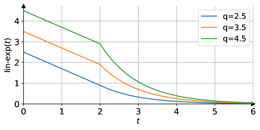
Figure 1: Plot of the linear-exponential function (6) with linear decay rate $c_{\textup{lin}}=0.8$, intercepts $q=\{2.5,\,3.5,\,4.5\}$, exponential decay rate $c_{\textup{exp}}=1$, and linear-exponential crossing time $t_{\textup{c}}=2$.

Before giving the main convergence results of this section, we prove the following:

Lemma III.1 (Property of the linear-exponential function):

Let $c_{\textup{exp}}$ and $d$ be positive scalars. Consider the dynamics

$$\dot{x}(t)=-c_{\textup{exp}}\operatorname{sat}_{d}({x(t)}),\quad x_{0}=q>d.$$ (7)

Then, $x(t)=\operatorname{lin-exp}({t\;;\;q,c_{\textup{lin}},c_{\textup{exp}},t_{\textup{c}}})$, with $c_{\textup{lin}}=dc_{\textup{exp}}$ and $t_{\textup{c}}:=qc_{\textup{lin}}^{-1}-c_{\textup{exp}}^{-1}>0$, is a solution of (7).

• First, we note that being the right end side of (7) locally Lipschitz continuous, the ODE (7) admits a unique continuous solution at least within a certain neighborhood of the initial condition.

  Using the definition of saturation function, for all $t\in\mathbb{R}_{\geq 0}$ we can write the ODE (7) as

  $$\dot{x}(t)=\begin{cases}dc_{\textup{exp}}&\textup{ if }x(t)<-d,\\ -c_{\textup{exp}}x(t)&\textup{ if }x(t)\in[-d,d],\\ -dc_{\textup{exp}}&\textup{ if }x(t)>d,\\ \end{cases}$$ (8)

  which, in each interval $[t_{0},t_{1}]\subseteq\mathbb{R}_{\geq 0}$ where the solution is continuous and does not change regime, has general solution

  $$x(t)=\begin{cases}dc_{\textup{exp}}t+x(t_{0})&\textup{ if }x(t)<-d,\\ x(t_{0})e^{-c_{\textup{exp}}(t-t_{0})}&\textup{ if }x(t)\in[-d,d],\\ -dc_{\textup{exp}}t+x(t_{0})&\textup{ if }x(t)>d.\\ \end{cases}$$ (9)

  At time $t=0$, we have $x_{0}=q>d$. For continuity of the solution, there exists $t^{\star}$ such that $x(t)>d$ for all $t\in[0,t^{\star}]$. Thus from (9) and being $x(t_{0}=0)=q$, it is $x(t)=-dc_{\textup{exp}}t+q$, for all $t\in[0,t^{\star}]$. Moreover being $x(t)$ a decreasing function, the time value $t^{\star}$ is finite and there exists a time, say it $\bar{t}$ such that $x(\bar{t})=d$. Let $c_{\textup{lin}}:=dc_{\textup{exp}}$, we have

  $$x(\bar{t})=d\iff-dc_{\textup{exp}}\bar{t}+q=d\iff\bar{t}=qc_{\textup{lin}}^{-1}-c_{\textup{exp}}^{-1}:=t_{\textup{c}}.$$

  In summary, we have shown that the solution of (8) is equal to $x(t)=q-c_{\textup{lin}}t$ for all $t\in[0,t_{\textup{c}}]$ and is equal to $d$ at time $t_{\textup{c}}$. Therefore from (9) and being $x(t_{\textup{c}})=q-c_{\textup{lin}}t_{\textup{c}}$, for all time $t>t_{\textup{c}}$ we have $x(t)=\bigl{(}q-c_{\textup{lin}}t_{\textup{c}}\bigr{)}e^{-c_{\textup{exp}}(t-t_{\textup{c}})}$. Specifically, $x(t)>0$ for all $t>t_{\textup{c}}$, thus it can never be the case $x(t)<-d$. This concludes the proof. ∎

Next, we study the convergence behavior of GW-LS-C systems of the form of (4), where the function $f\colon\mathbb{R}_{\geq 0}\times\mathcal{C}\rightarrow\mathbb{R}^{n}$ is locally Lipschitz and with $\mathcal{C}\subseteq\mathbb{R}^{n}$ being $f$-invariant, open and convex. In what follows, we make the following: There exist $\|\cdot\|_{\textup{G}},\|\cdot\|_{\textup{L}}$ on $\mathbb{R}^{n}$ such that

1. $f$ is weakly infinitesimally contracting on $\mathbb{R}^{n}$ w.r.t. $\|\cdot\|_{\textup{G}}$;

2. $f$ is $c_{\textup{exp}}$-strongly infinitesimally contracting on a forward-invariant set $\mathcal{S}$ w.r.t. $\|\cdot\|_{\textup{L}}$;

3. $x^{\star}\in\mathcal{S}$ is an equilibrium point, i.e., $f(t,x^{\star})=\mbox{0}_{n}$, for all $t\geq 0$.

Remark III.2:

Assumptions ($A$2), ($A$3) can be equivalently replaced by assuming the existence of a locally exponentially stable equilibrium. ∎

First, we consider GW-LS-C systems with respect to the same norm. Then, dynamics that are GW-LS-C with respect to different norms. In both scenarios, we show that the convergence is (globally) linear-exponential. That is, given a trajectory $x(t)$ of the dynamics, the distance $\|x(t)-x^{\star}\|_{\textup{G}}$ is upper bounded by a linear-exponential function (6).

III-A Convergence of Globally-Weakly and Locally-Strongly Contracting Dynamics with Respect to the Same Norm

We start by giving a bound on the upper right Dini derivative of the distance of any solution of (4) with respect to the equilibrium $x^{\star}$.

Lemma III.3 (Saturated error dynamics):

Consider system (4) and let Assumptions ($A$1) – ($A$3) hold with $\|\cdot\|_{\textup{G}}=\|\cdot\|_{\textup{L}}:=\|\cdot\|$. Let $r$ be the largest radius such that $B{\bigl{(}x^{\star},r\bigr{)}}\subseteq\mathcal{S}$. Then, for every trajectory $x(t)$ starting from $x_{0}\notin\mathcal{S}$, a.e. $t\geq 0$, we have

$$D^{+}\|x(t)-x^{\star}\| \leq-c_{\textup{exp}}\operatorname{sat}_{r}(\|x(t)-x^{\star}\|).$$ (10)

• Consider an arbitrary trajectory $x(t)$ starting from $x_{0}\notin\mathcal{S}$ and a second trajectory equal to the equilibrium $x^{\star}$. Let $\mu$ be the log-norm associated to $\|\cdot\|$. For a.e. $t\geq 0$ it holds ([6, 9]):

  $$D^{+}\|x(t)-x^{\star}\|\leq\int_{0}^{1}\mu\Bigl{(}D{f}\bigl{(}t,x^{\star}+\alpha(x(t)-x^{\star})\bigr{)}\Bigr{)}d\alpha\,\cdot\,\|x(t)-x^{\star}\|:=RHS.$$

  where $\alpha\in[0,1]$, and $x^{\star}+\alpha(x(t)-x^{\star})$ is the segment from $x^{\star}$ to $x(t)$.

  For each $t\geq 0$, if $\|x(t)-x^{\star}\|\leq r$, then Assumption ($A$2) implies

  $$RHS\leq\int_{0}^{1}(-c_{\textup{exp}})d\alpha\,\cdot\,\|x(t)-x^{\star}\|=-c_{\textup{exp}}\|x(t)-x^{\star}\|=-c_{\textup{exp}}\operatorname{sat}_{r}({\|x(t)-x^{\star}\|}),$$

  where in the last equality we have used the definition of saturation function. If $\|x(t)-x^{\star}\|\geq r$, define $\alpha^{*}=r/\|x(t)-x^{\star}\|$ and note that, a.e. $t\geq 0$, Assumptions ($A$2) and ($A$1) imply

  $$\alpha\leq\alpha^{*}\quad \implies\quad\mu\bigl{(}D{f}(t,x^{\star}+\alpha(x(t)-x^{\star}))\bigr{)}\leq-c_{\textup{exp}},$$

  $$\alpha>\alpha^{*}\quad \implies\quad\mu(D{f}(t,x^{\star}+\alpha(x(t)-x^{\star}))\bigr{)}\leq 0.$$

  Therefore, a.e. $t\geq 0$, it holds

  $$RHS \leq\Bigl{(}\int_{0}^{\alpha^{*}}\!\!\mu\bigl{(}D{f}(t,x^{\star}+\alpha(x(t)-x^{\star}))\bigr{)}d\alpha+\int_{\alpha^{*}}^{1}\!\!\mu\bigl{(}D{f}\bigl{(}t,x^{\star}+\alpha(x(t)-x^{\star}))\bigr{)}d\alpha\Bigr{)}\,\cdot\,\|x(t)-x^{\star}\|$$

  $$\leq(-c_{\textup{exp}}\alpha^{*}+0)\|x(t)-x^{\star}\|=-c_{\textup{exp}}r=-c_{\textup{exp}}\operatorname{sat}_{r}({\|x(t)-x^{\star}\|}),$$ (11)

  where in the last equality we used the definition of saturation function. This concludes the proof. ∎

We can now give our convergence result for GW-LS-C systems with respect to the same norm.

Theorem III.4 (Linear-exponential convergence of GW-LS-C systems w.r.t. the same norm):

Consider system (4) and let Assumptions ($A$1) – ($A$3) hold with $\|\cdot\|_{\textup{G}}=\|\cdot\|_{\textup{L}}:=\|\cdot\|$. Also, let $r$ be the largest radius such that $B{\bigl{(}x^{\star},r\bigr{)}}\subseteq\mathcal{S}$. For each trajectory $x(t)$ starting from $x_{0}$, it holds that

1. if $x_{0}\in\mathcal{S}$, then, a.e. $t\geq 0$,

   $$\|x(t)-x^{\star}\|\leq\mathrm{e}^{-c_{\textup{exp}}t}\|x_{0}-x^{\star}\|;$$

2. if $x_{0}\notin\mathcal{S}$, then, a.e. $t\geq 0$,

   $$\|x(t)-x^{\star}\|\leq\operatorname{lin-exp}({t\;;\;q,c_{\textup{lin}},c_{\textup{exp}},t_{\textup{c}}}),$$ (12)

   with

   • exponential decay rate $c_{\textup{exp}}>0$;

   • linear decay rate $c_{\textup{lin}}=c_{\textup{exp}}\,r$;

   • intercept $\displaystyle q=\|x_{0}-x^{\star}\|$;

   • linear-exponential crossing time $t_{\textup{c}}={(q-r)}/{c_{\textup{lin}}}$.

• Item (i) follows from Assumption ($A$2). Item (ii) follows by using the Comparison Lemma [13, pp. 102-103] to upper bound the solution to the differential inequality (10). Additionally, the upper bound obeys precisely the initial value (7) in Lemma III.1, for parameter values $d=r$, $c_{\textup{lin}}=c_{\textup{exp}}r$, $q=\|x_{0}-x^{\star}\|$, and $t_{\textup{c}}={(q-r)}/{c_{\textup{lin}}}$. This concludes the proof. ∎

III-B Convergence of Globally-Weakly and Locally-Strongly Contracting Dynamics with Respect to Different Norms

We begin by introducing the $\rho$-contraction time, where $0<\rho<1$.

Definition 4 ($\rho$-contraction time):

Let system (4) be strongly infinitesimally contracting with respect to a norm $\|\cdot\|_{\alpha}$. Consider the contraction factor $0<\rho<1$, a norm $\|\cdot\|_{\beta}$, and a vector $x\in\mathbb{R}^{n}$.

• The $\rho$-contraction time is the time required for each trajectory starting in $B_{\alpha}{\bigl{(}x,r\bigr{)}}$, for some $r>0$, to be inside $B_{\alpha}{\bigl{(}x,\rho r\bigr{)}}$;

• The $\rho$-contraction time with respect to $\|\cdot\|_{\beta}$ is the time required for each trajectory starting in $B_{\beta}{\bigl{(}x,r\bigr{)}}$, for some $r>0$, to be inside $B_{\beta}{\bigl{(}x,\rho r\bigr{)}}$.

Remark III.5:

It is implicit in Definition 4 that the $\rho$-contraction time for a specific trajectory depends on the initial condition and the center of the ball. ∎

We can now give our convergence result for GW-LS-C systems with respect to the different norms.

Theorem III.6 (Linear-exponential convergence of GW-LS-C systems):

Let $\|\cdot\|_{\textup{L}}$ and $\|\cdot\|_{\textup{G}}$ be two norms on $\mathbb{R}^{n}$ with equivalence ratio $k_{\textup{L},\textup{G}}$. Consider system (4) satisfying Assumptions ($A$1) – ($A$3). Let $r$ be the largest radius such that $B_{\textup{G}}{\bigl{(}x^{\star},r\bigr{)}}\subseteq\mathcal{S}$. For each trajectory $x(t)$ starting from $x_{0}$, it holds that

1. if $x_{0}\in\mathcal{S}$, then, a.e. $t\geq 0$,

   $$\|x(t)-x^{\star}\|_{\textup{G}}\leq k_{\textup{L},\textup{G}}\mathrm{e}^{-c_{\textup{exp}}t}\|x_{0}-x^{\star}\|_{\textup{G}};$$ (13)

2. if $x_{0}\notin\mathcal{S}$, then for any contractor factor $0<\rho<1$ and, a.e. $t\geq 0$,

   $$\|x(t)-x^{\star}\|_{\textup{G}} \leq\operatorname{lin-exp}({t\;;\;q,c_{\textup{lin}},c_{\textup{exp}},t_{\textup{c}}}),$$ (14)

   with

   • exponential decay rate $c_{\textup{exp}}>0$;

   • linear decay rate $c_{\textup{lin}}=c_{\textup{exp}}r(1-\rho)/\ln(k_{\textup{L},\textup{G}}\rho^{-1})$;

   • intercept $\displaystyle q=\|x_{0}-x^{\star}\|_{\textup{G}}+r(1-\rho)\frac{\ln(k_{\textup{L},\textup{G}})}{\ln(k_{\textup{L},\textup{G}}\rho^{-1})}$;

   • linear-exponential crossing time $t_{\textup{c}}=\left\lceil\frac{\|x_{0}-x^{\star}\|_{\textup{G}}-r}{(1-\rho)r}\right\rceil{\ln(k_{\textup{L},\textup{G}}\rho^{-1})}/{c_{\textup{exp}}}+\ln(k_{\textup{L},\textup{G}})/c_{\textup{exp}}$.

• Consider a trajectory $x(t)$ starting from initial condition $x_{0}$. If $x_{0}\in\mathcal{S}$, then item 13 follows from assumption ($A$2) and the equivalence of norms.

  Indeed, Assumption ($A$2) implies that for every $x_{0}\in\mathcal{S}$ and a.e. $t\geq 0$, it holds

  $$\|\phi_{t}\bigl{(}{x_{0}}\bigr{)}-x^{\star}\|_{\textup{L}}\leq\mathrm{e}^{-c_{\textup{exp}}t}\|x_{0}-x^{\star}\|_{\textup{L}}.$$

  Applying the equivalence of norms to the above inequality, we get

  $$\|\phi_{t}\bigl{(}{x_{0}}\bigr{)}-x^{\star}\|_{\textup{G}}\leq k_{\textup{L},\textup{G}}\mathrm{e}^{-c_{\textup{exp}}t}\|x_{0}-x^{\star}\|_{\textup{G}}.$$ (15)

  If $x_{0}\notin\mathcal{S}$, define the point $y_{0}:=x^{\star}+r\frac{x_{0}-x^{\star}}{\|x_{0}-x^{\star}\|_{\textup{G}}}\in\partial B_{\textup{G}}{\bigl{(}x^{\star},r\bigr{)}}$. The norm $\|y_{0}-x^{\star}\|_{\textup{G}}=r$, therefore $y_{0}$ is a point on the boundary of $B_{\textup{G}}{\bigl{(}x^{\star},r\bigr{)}}$. Moreover, the points $x^{\star}$, $y_{0}$, and $x_{0}$ lie on the same line segment, thus

  $$\|x_{0}-x^{\star}\|_{\textup{G}}=\|x_{0}-y_{0}\|_{\textup{G}}+r.$$ (16)

  By Lemma A.2(ii) and because each trajectory originating in $B_{\textup{G}}{\bigl{(}x^{\star},r\bigr{)}}$ remains in $\mathcal{S}$, the $\rho$-contraction with respect to $\|\cdot\|_{\textup{G}}$ for the $c_{\textup{exp}}$-strongly contracting vector field $f$ is

  $$t_{\rho}^{\textup{L},\textup{G}}=\frac{\ln(k_{\textup{L},\textup{G}}\rho^{-1})}{c_{\textup{exp}}}.$$ (17)

  Then, a.e. $t\in[0,t_{\rho}^{\textup{L},\textup{G}}]$, we have

  $$\|\phi_{t}\bigl{(}{x_{0}}\bigr{)}-x^{\star}\|_{\textup{G}} \leq\|\phi_{t}\bigl{(}{x_{0}}\bigr{)}-\phi_{t}(y_{0})\|_{\textup{G}}+\|\phi_{t}(y_{0})-x^{\star}\|_{\textup{G}}$$ (18)

  $$\leq\|x_{0}-y_{0}\|_{\textup{G}}+k_{\textup{L},\textup{G}}\mathrm{e}^{-c_{\textup{exp}}t}\|y_{0}-x^{\star}\|_{\textup{G}}$$ (19)

  $$\overset{\eqref{eq:aligned_points}}{=}\|x_{0}-x^{\star}\|_{\textup{G}}-\|x^{\star}-y_{0}\|_{\textup{G}}+k_{\textup{L},\textup{G}}\mathrm{e}^{-c_{\textup{exp}}t}r$$

  $$\!\!\!\overset{t=t_{\rho}^{\textup{L},\textup{G}}}{\leq}\|x_{0}-x^{\star}\|_{\textup{G}}-r(1-k_{\textup{L},\textup{G}}\mathrm{e}^{-c_{\textup{exp}}{t_{\rho}^{\textup{L},\textup{G}}}})$$

  $$\overset{\eqref{eq:rho_time_proof}}{=}\|x_{0}-x^{\star}\|_{\textup{G}}-r(1-\rho),$$ (20)

  where in (18) we added and subtracted $\phi_{t}(y_{0})$ and applied the triangle inequality, while inequality (19) follows from Assumption ($A$1) and inequality (15). Now, (20) implies that $\|\phi_{t_{\rho}^{\textup{L},\textup{G}}}\bigl{(}{x_{0}}\bigr{)}-x^{\star}\|_{\textup{G}}\leq\|x_{0}-x^{\star}\|_{\textup{G}}-r(1-\rho)$. If $\|x_{0}-x^{\star}\|_{\textup{G}}-r(1-\rho)\leq r$, then by Assumption ($A$2), a.e. in $t\geq t_{\rho}^{\textup{L},\textup{G}}$, we have

  $$\|\phi_{t}\bigl{(}{x_{0}}\bigr{)}-x^{\star}\|_{\textup{G}} \leq k_{\textup{L},\textup{G}}\mathrm{e}^{-c_{\textup{exp}}(t-t_{\rho}^{\textup{L},\textup{G}})}\bigl{(}\|x_{0}-x^{\star}\|_{\textup{G}}-r(1-\rho)\bigr{)}.$$

  If $\|x_{0}-x^{\star}\|_{\textup{G}}-r(1-\rho)>r$, we iterate the process. Specifically, let $x_{\rho}:=\phi_{t_{\rho}^{\textup{L},\textup{G}}}(x_{0})$, and define $\displaystyle y_{\rho}:=x^{\star}+r\frac{x_{\rho}-x^{\star}}{\|x_{\rho}-x^{\star}\|_{\textup{G}}}\in\partial B_{\textup{G}}{\bigl{(}x^{\star},r\bigr{)}}$. Consider the solution to $\dot{y}=f(t,y)$ with initial condition $y({t_{\rho}^{\textup{L},\textup{G}}})=y_{\rho}$ and note that $\phi_{t}(x_{\rho})=\phi_{t+t_{\rho}^{\textup{L},\textup{G}}}(x_{0})$. For a.e. $t\in[t_{\rho}^{\textup{L},\textup{G}},2t_{\rho}^{\textup{L},\textup{G}}]$, we compute

  $$\|\phi_{t+t_{\rho}^{\textup{L},\textup{G}}}(x_{0})-x^{\star}\|_{\textup{G}} \leq\|\phi_{t}(x_{\rho})-\phi_{t}(y_{\rho})\|_{\textup{G}}+\|\phi_{t}(y_{\rho})-x^{\star}\|_{\textup{G}}$$ (21)

  $$\leq\|x_{\rho}-y_{\rho}\|_{\textup{G}}+k_{\textup{L},\textup{G}}\mathrm{e}^{-c(t-t_{\rho}^{\textup{L},\textup{G}})}\|y_{0}-x^{\star}\|_{\textup{G}}$$ (22)

  $$\!\!\overset{\eqref{eq:aligned_points}}{=}\|x_{\rho}-x^{\star}\|_{\textup{G}}-\|x^{\star}-y_{\rho}\|_{\textup{G}}+k_{\textup{L},\textup{G}}\mathrm{e}^{-c(t-t_{\rho}^{\textup{L},\textup{G}})}r$$

  $$\leq\|\phi_{t_{\rho}^{\textup{L},\textup{G}}}(x_{0})-x^{\star}\|_{\textup{G}}-r(1-k_{\textup{L},\textup{G}}\mathrm{e}^{-c(t-t_{\rho}^{\textup{L},\textup{G}})})$$

  $$\!\!\overset{\eqref{eq:decreasing1}}{\leq}\|x_{0}-x^{\star}\|_{\textup{G}}-r(1-\rho)-r(1-k_{\textup{L},\textup{G}}\mathrm{e}^{-c(t-t_{\rho}^{\textup{L},\textup{G}})})$$

  $$\!\!\!\!\!\overset{t=2t_{\rho}^{\textup{L},\textup{G}}}{\leq}\|x_{0}-x^{\star}\|_{\textup{G}}-2r(1-\rho),$$

  where in (21) we added and subtracted $\phi_{t}(y_{0})$ and applied the triangle inequality, while (19) follows from Assumption ($A$1) and (15). We now reason as done in $[0,t_{\rho}^{\textup{L},\textup{G}}]$. If $\|x_{0}-x^{\star}\|_{\textup{G}}-2r(1-\rho)\leq r$, then Assumption ($A$2) implies

  $$\|\phi_{t+t_{\rho}^{\textup{L},\textup{G}}}(x_{0})-x^{\star}\|_{\textup{G}}\leq k_{\textup{L},\textup{G}}\bigl{(}\|x_{0}-x^{\star}\|_{\textup{G}}-2r(1-\rho)\bigr{)}\mathrm{e}^{-c(t-2t_{\rho}^{\textup{L},\textup{G}})},\quad\forall t\geq 2t_{\rho}^{\textup{L},\textup{G}}.$$

  If $\|x_{0}{-}x^{\star}\|_{\textup{G}}{-}2r(1{-}\rho)>r$, we proceed analogously until $\|x_{0}-x^{\star}\|_{\textup{G}}-Tr(1-\rho)\leq r$. This inequality is verified after at most $T:=\left\lceil\frac{\|x_{0}-x^{\star}\|_{\textup{G}}-r}{(1-\rho)r}\right\rceil$ steps. Iterating the previous process, at step $T$, for almost every $t\in[(T-1)t_{\rho}^{\textup{L},\textup{G}},Tt_{\rho}^{\textup{L},\textup{G}}]$, we get

  $$\|\phi_{t+(T-1)t_{\rho}^{\textup{L},\textup{G}}}(x_{0})-x^{\star}\|_{\textup{G}} \leq\|x_{0}-x^{\star}\|_{\textup{G}}-(T-1)r(1-\rho)-r(1-k_{\textup{L},\textup{G}}\mathrm{e}^{-c(t-(T-1)t_{\rho}^{\textup{L},\textup{G}})}),$$

  $$\!\!\!\!\overset{t=kt_{\rho}^{\textup{L},\textup{G}}}{\leq}\!\!\!\!\|x_{0}-x^{\star}\|_{\textup{G}}-Tr(1-\rho)\leq r,$$

  where the last inequality follows from the definition of $T$. Local strong contractivity then implies

  $$\|\phi_{t+Tt_{\rho}^{\textup{L},\textup{G}}}(x_{0})-x^{\star}\|_{\textup{G}}\leq k_{\textup{L},\textup{G}}\bigl{(}\|x_{0}-x^{\star}\|_{\textup{G}}-Tr(1-\rho)\bigr{)}\mathrm{e}^{-c(t-Tt_{\rho}^{\textup{L},\textup{G}})},\quad\text{ a.e. }t\geq Tt_{\rho}^{\textup{L},\textup{G}}.$$

  The above reasoning together with Assumption ($A$1) implies that a.e. $t\in[it_{\rho}^{\textup{L},\textup{G}},(i+1)t_{\rho}^{\textup{L},\textup{G}}]$, $i\in\{0,\dots,T-1\}$, we have

  $$\|\phi_{t+it_{\rho}^{\textup{L},\textup{G}}}(x_{0})-x^{\star}\|_{\textup{G}}\leq\min\Big{\{}\|x_{0}-x^{\star}\|_{\textup{G}}-ir(1-\rho),\|x_{0}-x^{\star}\|_{\textup{G}}-ir(1-\rho)-r\bigl{(}1-k_{\textup{L},\textup{G}}\mathrm{e}^{-c(t-i{t_{\rho}^{\textup{L},\textup{G}}})}\bigr{)}\Big{\}}.$$

  By partitioning the time interval $[0,+\infty[$ as $[0,t_{\rho}^{\textup{L},\textup{G}}[\cup\dots\cup[(T-1)t_{\rho}^{\textup{L},\textup{G}},Tt_{\rho}^{\textup{L},\textup{G}}[\cup[Tt_{\rho}^{\textup{L},\textup{G}},+\infty[$ and summing up the above inequalities we obtain the bound:

  $$\|\phi_{t}(x_{0})-x^{\star}\|_{\textup{G}} \leq\sum_{i=0}^{T-1}\mathbf{1}_{\{i{t_{\rho}^{\textup{L},\textup{G}}}\leq t<(i+1){t_{\rho}^{\textup{L},\textup{G}}}\}}(t)\cdot\min\Big{\{}\|x_{0}-x^{\star}\|_{\textup{G}}-ir(1-\rho),\|x_{0}-x^{\star}\|_{\textup{G}}-ir(1-\rho)$$

  $$\quad-r\bigl{(}1-k_{\textup{L},\textup{G}}\mathrm{e}^{-c(t-i{t_{\rho}^{\textup{L},\textup{G}}})}\bigr{)}\Big{\}}+\mathbf{1}_{\{t\geq T{t_{\rho}^{\textup{L},\textup{G}}}\}}(t)\cdot\min\Big{\{}\|x_{0}-x^{\star}\|_{\textup{G}}-Tr(1-\rho),$$

  $$\quad k_{\textup{L},\textup{G}}\left(\|x_{0}-x^{\star}\|_{\textup{G}}-Tr(1-\rho)\right)\mathrm{e}^{-c(t-T{t_{\rho}^{\textup{L},\textup{G}}})}\Big{\}}:=g_{\textup{B}}(t).$$ (23)

  Finally, item (ii) follows by noticing that $g_{\textup{B}}(t)\leq\operatorname{lin-exp}({t\;;\;q,c_{\textup{lin}},c_{\textup{exp}},t_{\textup{c}}})$, $t\geq 0$, for the values $t_{\textup{c}}=T{\ln(k_{\textup{L},\textup{G}}\rho^{-1})}/{c_{\textup{exp}}}+\ln(k_{\textup{L},\textup{G}})/c_{\textup{exp}}$, $c_{\textup{lin}}=r\,c_{\textup{exp}}(1-\rho)/\ln(k_{\textup{L},\textup{G}}\rho^{-1})$, and $\displaystyle q=\|x_{0}-x^{\star}\|_{\textup{G}}+r(1-\rho)\frac{\ln(k_{\textup{L},\textup{G}})}{\ln(k_{\textup{L},\textup{G}}\rho^{-1})}$. This concludes the proof. ∎

Remark III.7:

Theorem III.6 sharpens the convergence bound established in [4]. Namely, it provides a more accurate intercept and linear-exponential crossing time. An illustration between the bound in equation (14) and the one in [4] is given in Figure 2. ∎

Figure 2: Linear-exponential bound in equation (14) (solid blue curve) and the decay bound presented in [4] (red curve) for $\|x_{0}-x^{\star}\|_{\textup{G}}=2.4$, $r=1$, $c_{\textup{exp}}=1$, $k_{L,G}=2$, $\rho=0.4$.

Remark III.8:

The bound in Theorem III.6 generalizes the result for equal norms in Theorem III.4. In fact, the factor $(1-\rho)/\ln(k_{\textup{L},\textup{G}}\rho^{-1})$ is always less than 1 for $k_{\textup{L},\textup{G}}>1$. Moreover, when $k_{\textup{L},\textup{G}}=1$ it results $\displaystyle\lim_{\rho\to 1}(1-\rho)/\ln(k_{\textup{L},\textup{G}}\rho^{-1})=1$, thereby exactly recovering the equal-norm result. ∎

IV Local Stability in the Presence of External Inputs

We now characterize local ISS for GW-LS-C systems w.r.t. the same norm. Specifically, we consider the system

$$\dot{x}(t)=f\bigl{(}t,x(t),u(t)\bigr{)}.$$ (24)

where, $f\colon\mathbb{R}_{\geq 0}\times\mathcal{C}\times\mathcal{U}\rightarrow\mathbb{R}^{n}$, the map $x\mapsto f(t,x,u)$ is locally Lipschitz, for all $t$, $u$, with $\mathcal{C}\subseteq\mathbb{R}^{n}$ $f$-invariant, open and convex, and $\mathcal{U}\subset\mathbb{R}^{m}$. Given $\bar{u}\in\mathbb{R}^{m}$, we define the set of bounded inputs $\bar{\mathcal{U}}:=\{u\colon\mathbb{R}_{\geq 0}\rightarrow\mathcal{U}\;|\;\|u(t)\|_{\mathcal{U}}\leq\bar{u},\forall t\geq 0\}$. We make the following: there exist norms $\|\cdot\|,\|\cdot\|_{\mathcal{U}}$ on $\mathcal{C}$ and $\mathcal{U}$, respectively, such that

1. for all $t$, $u$, the map $x\mapsto f(t,x,u)$ is weakly infinitesimally contracting on $\mathbb{R}^{n}$ w.r.t. $\|\cdot\|$;

2. for all $t$, $x$, the map $u\mapsto f(t,x,u)$ is Lipschitz with constant $L_{u}\geq 0$;

3. there exist a forward-invariant set $\mathcal{S}$ and $c_{\textup{exp}}>0$ such that, for all $t$, for each $u\in\bar{\mathcal{U}}$, the map $x\mapsto f(t,x,u(t))$ is $c_{\textup{exp}}$-strongly infinitesimally contracting on $\mathcal{S}$ w.r.t. $\|\cdot\|$;

4. at $u(t)=\mbox{0}_{m}$, for all $t$, there exists an equilibrium point $x^{\star}\in\mathcal{S}$.

We begin by giving two technical lemmas, needed to prove the main result of this section.

Lemma IV.1 (Error dynamics for input-dependent systems):

Consider system (24) satisfying Assumption ($A$2’). Then any two solutions $x(t)$ and $y(t)$ with input $u_{x},u_{y}\colon\mathbb{R}_{\geq 0}\rightarrow\mathbb{R}^{m}$, satisfy a.e. $t\geq 0$,

$$D^{+}\|x(t)-y(t)\| \leq\int_{0}^{1}\mu\Bigl{(}Df(y+\alpha(x-y),u_{y})\Bigr{)}d\alpha\|x(t)-y(t)\|+L_{u}\|u_{x}(t)-u_{y}(t)\|_{\mathcal{U}}.$$ (25)

• Let $x(t)$ and $y(t)$ be two trajectories of (24) with input signals $u_{x},u_{y}$, respectively. Let $\left\llbracket{\cdot},{\cdot}\right\rrbracket$ be a weak pairing compatible with $\|\cdot\|$. We compute

  $$\|x(t)-y(t)\| D^{+}\|x(t)-y(t)\|=\left\llbracket{f(t,x,u_{x})-f(t,y,u_{y})},{x-y}\right\rrbracket$$ (26)

  $$\leq\left\llbracket{f(t,x,u_{y})-f(t,y,u_{y})},{x-y}\right\rrbracket+\|f(t,x,u_{x})-f(t,x,u_{y})\|\|x-y\|$$ (27)

  $$\leq\left\llbracket{f(t,x,u_{y})-f(t,y,u_{y})},{x-y}\right\rrbracket+L_{u}\|u_{x}-u_{y}\|_{\mathcal{U}}\|x-y\|,$$ (28)

  where in (26) we used the curve norm derivative formula (ii), in (27) we added and subtracted $f(t,x,u_{y})$ and used the sub-additivity (i) and the Cauchy-Schwartz inequality (iii), and in (28) we used Assumption ($A$2’).

  Next, by dividing both side for $\|x(t)-y(t)\|$ we get

  $$D^{+}\|x(t)-y(t)\| \leq\frac{\left\llbracket{f(t,x,u_{y})-f(t,y,u_{y})},{x-y}\right\rrbracket}{\|x-y\|}+L_{u}\|u_{x}-u_{y}\|_{\mathcal{U}}$$

  $$=\frac{\left\llbracket{f(t,x,u_{y})-f(t,y,u_{y})},{x-y}\right\rrbracket}{\|x-y\|^{2}}\|x-y\|+L_{u}\|u_{x}-u_{y}\|_{\mathcal{U}}.$$ (29)

  By applying the mean-value Theorem II.1 to (29), a.e., we get

  $$D^{+}\|x(t)-y(t)\| \leq\frac{\left\llbracket{\int_{0}^{1}Df(y+s(x-y),u_{y})ds(x-y)},{x-y}\right\rrbracket}{\|x-y\|}\frac{\|x-y\|}{\|x-y\|}+L_{u}\|u_{x}-u_{y}\|_{\mathcal{U}}$$ (30)

  $$\leq\int_{0}^{1}\frac{\left\llbracket{Df(y+s(x-y),u_{y})ds(x-y)},{x-y}\right\rrbracket}{\|x-y\|^{2}}ds\|x-y\|+L_{u}\|u_{x}-u_{y}\|_{\mathcal{U}},$$ (31)

  where in (30) we have used the weak pairing sub-additivity (i). Next, recall that Lumer’s equality (iv) implies, $\displaystyle\frac{\left\llbracket{Az},{z}\right\rrbracket}{\left\llbracket{z},{z}\right\rrbracket}\leq\mu\bigl{(}A\bigr{)}$ for every $A\in\mathbb{R}^{n\times n}$ and $z\neq\mbox{0}_{n}$. By applying this equality to (31) (with $A=Df(y+s(x-y),u_{y})$ and $z=x-y$) we get inequality (25). This concludes the proof. ∎

The next result gives a linear-exponential bound for the solution of dynamics with saturations and additive inputs.

Lemma IV.2 (Solution of dynamics with saturations and additive inputs):

Let $c_{\textup{exp}}$ and $d$ be positive scalars, and $u\colon\mathbb{R}_{\geq 0}\rightarrow\mathbb{R}^{n}$ satisfying $\displaystyle\|u(t)\|_{\infty}=u_{\textup{max}}<dc_{\textup{exp}}$, for all $t$. Consider the dynamics

$$\dot{x}(t)=-c_{\textup{exp}}\operatorname{sat}_{d}({x(t)})+u(t),\quad x_{0}=q>d.$$ (32)

Then, a solution of (32) satisfies

$$x(t)\leq\operatorname{lin-exp}({t\;;\;q,c_{\textup{lin}},c_{\textup{exp}},t_{\textup{c}}})+\mathbf{1}_{[t_{\textup{c}},+\infty[}(t)(1-\mathrm{e}^{-c_{\textup{exp}}(t-t_{\textup{c}})})\frac{u_{\textup{max}}}{c_{\textup{exp}}},$$

with $c_{\textup{lin}}:=dc_{\textup{exp}}-u_{\textup{max}}>0$ and $t_{\textup{c}}:=\frac{q-d}{c_{\textup{lin}}}>0$.

• Using the definition of saturation function, for all $t\in\mathbb{R}_{\geq 0}$ we can upper bound the ODE (32) as

  $$\dot{x}(t)\leq\dot{y}(t):=\begin{cases}-dc_{\textup{exp}}+u_{\textup{max}}&\textup{ if }y(t)>d,\\ -c_{\textup{exp}}x(t)+u_{\textup{max}}&\textup{ if }y(t)\in[-d,d],\\ dc_{\textup{exp}}+u_{\textup{max}}&\textup{ if }y(t)<-d,\\ \end{cases}$$ (33)

  which, in each interval $[t_{0},t_{1}]\subseteq\mathbb{R}_{\geq 0}$ where the solution is continuous and does not change regime, has general solution

  $$y(t) =\begin{cases}\displaystyle(-dc_{\textup{exp}}+u_{\textup{max}})t+y(t_{0})&\textup{ if }y(t)>d,\\ \displaystyle\Bigl{(}y(t_{0})-\frac{\bar{u}}{c_{\textup{exp}}}\Bigr{)}\mathrm{e}^{-c_{\textup{exp}}(t-t_{0})}+\frac{u_{\textup{max}}}{c_{\textup{exp}}}&\textup{ if }y(t)\in[-d,d],\\ \displaystyle(dc_{\textup{exp}}+u_{\textup{max}})t+y(t_{0})&\textup{ if }y(t)<-d.\\ \end{cases}$$ (34)

  At time $t=0$, we have $x_{0}=q>d$. For continuity of the solution, there exists $t^{\star}$ such that $y(t)>d$ for all $t\in[0,t^{\star}]$. Thus from (34) and being $x(t_{0}=0)=q$, it is

  $$y(t)=(-dc_{\textup{exp}}+u_{\textup{max}})t+q,$$

  for all $t\in[0,t^{\star}]$. Moreover being $u_{\textup{max}}<dc_{\textup{exp}}$, the function $y(t)$ is decreasing, the time value $t^{\star}$ is finite and there exists a time, say it $\bar{t}$ such that $y(\bar{t})=d$. Let $c_{\textup{lin}}:=dc_{\textup{exp}}-u_{\textup{max}}$, we have

  $$y(\bar{t})=d\iff-c_{\textup{lin}}\bar{t}+q=d\iff\bar{t}=\frac{q-d}{c_{\textup{lin}}}:=t_{\textup{c}}.$$

  In summary, we have shown that $y(t)=q-c_{\textup{lin}}t$ for all $t\in[0,t_{\textup{c}}]$ and is equal to $d$ at time $t_{\textup{c}}$. Therefore from (34) and being $y(t_{\textup{c}})=q-c_{\textup{lin}}t_{\textup{c}}$, for all time $t>t_{\textup{c}}$ we have

  $$y(t)=\bigl{(}q-c_{\textup{lin}}t_{\textup{c}}\bigr{)}\mathrm{e}^{-c_{\textup{exp}}(t-t_{\textup{c}})}+\bigl{(}1-\mathrm{e}^{-c_{\textup{exp}}(t-t_{\textup{c}})}\bigr{)}\frac{u_{\textup{max}}}{c_{\textup{exp}}}.$$

  Specifically, $y(t)>0$ for all $t>t_{\textup{c}}$, thus it can never be $y(t)<-d$. This concludes the proof. ∎

We are now ready to state the following:

Theorem IV.3 (Local ISS for input-dependent GW-LS-C systems):

Consider system (24) satisfying Assumptions ($A$1’) – ($A$4’). Let $r$ be the largest radius such that $B{\bigl{(}x^{\star},r\bigr{)}}\subseteq\mathcal{S}$, $\bar{u}<rc_{\textup{exp}}$, and $u_{\textup{max}}:=\sup_{\tau\in[0,t]}\|u_{x}(\tau)\|_{\mathcal{U}}\leq\bar{u}$. For each trajectory $x(t)$ with input $u_{x}\in\bar{\mathcal{U}}$ starting from $x_{0}\notin\mathcal{S}$, a.e. $t\geq 0$, we have:

1. $\displaystyle D^{+}\|x(t){-}x^{\star}\|\leq-c_{\textup{exp}}\operatorname{sat}_{r}(\|x(t){-}x^{\star}\|){+}L_{u}\|u_{x}(t)\|_{\mathcal{U}};$

2. $\displaystyle\|x(t){-}x^{\star}\|\leq\operatorname{lin-exp}({t\;;\;q,c_{\textup{lin}},c_{\textup{exp}},t_{\textup{c}}})+\mathbf{1}_{[t_{\textup{c}},+\infty[}(t)\frac{L_{u}}{c_{\textup{exp}}}(1-\mathrm{e}^{-c_{\textup{exp}}t})u_{\textup{max}},$

   with

   • exponential decay rate $c_{\textup{exp}}>0$;

   • intercept $\displaystyle q=\|x_{0}-x^{\star}\|$;

   • linear decay rate $c_{\textup{lin}}=rc_{\textup{exp}}-u_{\textup{max}}$;

   • linear-exponential crossing time $t_{\textup{c}}={(q-r)}/{c_{\textup{lin}}}$.

• Consider an arbitrary trajectory $x(t)$ starting from $x_{0}\notin\mathcal{S}$ with input $u_{x}$ and a second trajectory equal to the equilibrium $x^{\star}$ with input $u=\mbox{0}_{m}$. To prove statement (i), let $\mu$ be the log-norm associated to $\|\cdot\|$. By applying inequality (25) to those trajectories, a.e. $t\geq 0$, we have

  $$D^{+}\|x(t)-x^{\star}\| \leq\int_{0}^{1}\mu\Bigl{(}Df(x^{\star}+\alpha(x(t)-x^{\star}),0)\Bigr{)}d\alpha\|x(t)-x^{\star}\|+L_{u}\|u_{x}\|_{\mathcal{U}}.$$ (35)

  The proof follows by using similar reasoning as the one in the proof of Lemma III.3. Item (ii) follows by using the Comparison Lemma [13, pp. 102-103] and Lemma IV.2 to upper bound the solution to the differential inequality (i). ∎

V Tackling Linear Programs

We now show the efficacy of the previous results by applying them to a dynamical system solving the LP problem. Given $c\in\mathbb{R}^{n}$, $A\in\mathbb{R}^{m\times n}$ and $b\in\mathbb{R}^{m}$, we consider the linear program:

$$\min_{x\in\mathbb{R}^{n}} c^{\top}x,$$ (36)

s.t. $$Ax\leq b,$$

and its equivalent unconstrained formulation

$$\min_{x\in\mathbb{R}^{n}}c^{\top}x+\iota_{\mathcal{I}_{b}}(Ax),$$ (37)

where $\mathcal{I}_{b}=\{y\in\mathbb{R}^{m}\;|\;y-b\leq\mbox{0}_{m}\}$. We assume that (37) admits a unique equilibrium. Note that (37) is a particular composite minimization problem:

$$\min_{x\in\mathbb{R}^{n}}f(x)+g(Ax),$$ (38)

with $f(x)=c^{\top}x$ and $g(Ax)=\iota_{\mathcal{I}_{b}}(Ax)$. To solve (37), we leverage the proximal augmented Lagrangian approach proposed in [10] and consider the proximal augmented Lagrangian, $\tilde{L}_{\gamma}\colon\mathbb{R}^{n}\times\mathbb{R}^{m}\rightarrow\mathbb{R}$, defined by

$$\tilde{L}_{\gamma}(x,\lambda)=f(x)+M_{\gamma g}(Ax+\gamma\lambda)-\frac{\gamma}{2}\|\lambda\|_{2}^{2},$$ (39)

where $\lambda\in\mathbb{R}^{m}$ is the Lagrange multiplier, $\gamma>0$ is a parameter, and $M_{\gamma g}$ is Moreau envelope of $g$.

Remark V.1:

For $f$ continuously differentiable, convex, and with a Lipschitz continuous gradient, and $g$ convex, closed and proper, solving the composite minimization problem (38) corresponds to finding saddle points of (39), simultaneously updating the primal and dual variables [10, Theorem 2]. ∎

Next, consider the continuous-time augmented primal-dual dynamics [10] (that can be interpreted as a continuous-time neural network) associated to the proximal augmented Lagrangian of problem (37)

$$\dot{x} =-\nabla_{x}\tilde{L}_{\gamma}(x,\lambda)=-c-A^{\top}\nabla M_{\gamma\iota_{\mathcal{I}_{b}}}(Ax+\gamma\lambda)=-c-\frac{1}{\gamma}A^{\top}\operatorname{ReLU}\bigl{(}Ax+\gamma\lambda-b\bigr{)},$$ (40)

$$\dot{\lambda} =\nabla_{\lambda}\tilde{L}_{\gamma}(x,\lambda)=-\gamma\lambda+\gamma\nabla M_{\gamma\iota_{\mathcal{I}_{b}}}(Ax+\gamma\lambda)=-\gamma\lambda+\operatorname{ReLU}\bigl{(}Ax+\gamma\lambda-b\bigr{)}.$$

We let $F_{\textup{LP}}\colon\mathbb{R}^{n+m}\rightarrow\mathbb{R}^{n+m}$ denote the vector field for (40).

Remark V.2:

Equation (40) follows directly after noticing that for a.e. $y\in\mathbb{R}^{m}$ it results

$$\nabla M_{\gamma\iota_{\mathcal{I}}}(y) =\frac{1}{\gamma}\bigl{(}y-\mathbb{P}_{\iota_{\mathcal{I}}}(y)\bigr{)}=\frac{1}{\gamma}\bigl{(}y-\min\{y,b\}\bigr{)}=\frac{1}{\gamma}\operatorname{ReLU}\bigl{(}y-b\bigr{)}.$$

∎

The next result characterizes the convergence of (40).

Theorem V.3 (Convergence of the linear program):

Consider the dynamics (40) and let $(x^{\star},\lambda^{\star})\in\mathbb{R}^{n+m}$ be an equilibrium point. If $DF_{\textup{LP}}\bigl{(}x^{\star},\lambda^{\star})$ is Hurwitz, then any solution of (40) linear-exponentially converges towards $(x^{\star},\lambda^{\star})$.

• To prove the statement we show that (40) satisfies the assumptions of Theorem III.6. First, we prove that the system is globally-weakly contracting. To this purpose, let $z:=(x,\lambda)\in\mathbb{R}^{n+m}$, $y:=Ax+\gamma\lambda-b$ and define $G(y):=D\operatorname{ReLU}\bigl{(}y\bigr{)}$, a.e. $y\in\mathbb{R}^{m}$. The Jacobian of (40) is

  $$DF_{\textup{LP}}(z)=\begin{bmatrix}-\frac{1}{\gamma}A^{\top}G(y)A&\!\!-A^{\top}G(y)\\ G(y)A&\!\!-\gamma(I_{m}-G(y))\end{bmatrix}.$$

  Being $0\preceq G(y)\preceq I_{m}$, a.e. $y\in\mathbb{R}^{m}$, we have

  $$\sup_{z}\mu_{2}\bigl{(}DF_{\textup{LP}}(z)\bigr{)}\leq\max_{0\preceq G\preceq I_{m}}\mu_{2}\left(\begin{bmatrix}-\gamma^{-1}A^{\top}GA&-A^{\top}G\\ GA&\gamma\bigl{(}G-I_{m}\bigr{)}\end{bmatrix}\right),$$

  By definition of $\mu_{2}$, we have that

  $$\mu_{2}\left(\begin{bmatrix}-\gamma^{-1}A^{\top}GA&-A^{\top}G\\ GA&\gamma\bigl{(}G-I_{m}\bigr{)}\end{bmatrix}\right) =\lambda_{\textup{max}}\Biggl{(}\begin{bmatrix}-\gamma^{-1}A^{\top}GA&0\\ 0&\gamma\bigl{(}G-I_{m}\bigr{)}\end{bmatrix}\Biggr{)}$$

  $$=\max\{\lambda_{\textup{max}}\bigl{(}-\gamma^{-1}A^{\top}GA\bigr{)},\lambda_{\textup{max}}\bigl{(}\gamma\bigl{(}G-I_{m}\bigr{)}\bigr{)}\}\leq 0.$$

  The last equality follows from the fact that $\lambda_{\textup{max}}\bigl{(}-\gamma^{-1}A^{\top}GA\bigr{)}=\lambda_{\textup{max}}\bigl{(}\gamma\bigl{(}G-I_{m}\bigr{)}\bigr{)}\leq 0$. In particular, the equality $\lambda_{\textup{max}}\bigl{(}-\gamma\bigl{(}G-I_{m}\bigr{)}\bigr{)}\leq 0$ follows directly from $0\preceq G\preceq I_{m}$; while $\lambda_{\textup{max}}\bigl{(}-\gamma^{-1}A^{\top}GA\bigr{)}\leq 0$, follows noticing that $A^{\top}GA\succeq 0$. This implies that (40) is weakly contracting on $\mathbb{R}^{n+m}$ w.r.t. $\|\cdot\|_{2}$. Next, we prove that the system is locally-strongly contracting. To do so, we first note that for any equilibrium point $z^{\star}:=(x^{\star},\lambda^{\star})$ of (40), the KKT conditions implies that $y^{\star}:=Ax^{\star}+\gamma\lambda^{\star}-b\neq\mbox{0}_{m}$. This in turn implies that both $D\operatorname{ReLU}(y^{\star})$ and $DF_{\textup{LP}}(z^{\star})$ are well defined. Now, being by assumption $DF_{\textup{LP}}(z^{\star})$ Hurwitz, there exists $Q$ invertible such that $\mu_{2,Q}\bigl{(}DF_{\textup{LP}}(z^{\star})\bigr{)}<0$ [3, Corollary 2.33]. Let $\mathcal{K}$ be the set of differentiable points in a neighborhood of $z^{\star}$. Then, by the continuity property of the log-norm, there exists $B_{2,Q}{\bigl{(}z^{\star},p\bigr{)}}$, with $p:=\sup\{p>0\;|\;B_{2,Q}{\bigl{(}z^{\star},p\bigr{)}}\subset\mathcal{K}\}$, where $DF_{\textup{LP}}(z)$ exists and $\mu_{2,Q}\bigl{(}DF_{\textup{LP}}(z)\bigr{)}<-c_{\textup{exp}}$ for all $z\in B_{2,Q}{\bigl{(}z^{\star},p\bigr{)}}$, for some $c_{\textup{exp}}>0$. Therefore (40) is strongly infinitesimally contracting w.r.t. $\|\cdot\|_{2,Q}$ in $B_{2,Q}{\bigl{(}z^{\star},p\bigr{)}}$. This concludes the proof. ∎

A key hypothesis in Theorem V.3 is that $DF_{\textup{LP}}\bigl{(}x^{\star},\lambda^{\star})$ is Hurwitz. To this aim, we make the following:

Conjecture V.4:

Let $(x^{\star},\lambda^{\star})$ be the equilibrium of (40). The LP (36) has a unique solution, $x^{\star}$, if and only if $DF_{\textup{LP}}\bigl{(}x^{\star},\lambda^{\star})$ is Hurwitz.

Numerical Experiments

Consider the following LP

$$\min_{x\in\mathbb{R}^{3}} x_{1}+x_{2}+x_{3},$$ (41)

s.t. $$-1\leq x_{1}\leq 1,-1\leq x_{2}\leq 1,-1\leq x_{3}\leq 1.$$

for which the unique optimal solution is $x^{\star}=(-1,-1,-1)$.

Next, consider the corresponding continuous-time augmented primal-dual dynamics (40)

$$\dot{x}_{1} =-1-\frac{1}{\gamma}\Bigl{(}\operatorname{ReLU}\left(x_{1}+\gamma\lambda_{1}-1\right)-\operatorname{ReLU}\left(-x_{1}+\gamma\lambda_{4}-1\right)\Bigr{)},$$ (42)

$$\dot{x}_{2} =-1-\frac{1}{\gamma}\Bigl{(}\operatorname{ReLU}\left(x_{2}+\gamma\lambda_{2}-1\right)-\operatorname{ReLU}\left(-x_{2}+\gamma\lambda_{5}-1\right)\Bigr{)},$$

$$\dot{x}_{3} =-1-\frac{1}{\gamma}\Bigl{(}\operatorname{ReLU}\left(x_{3}+\gamma\lambda_{3}-1\right)-\operatorname{ReLU}\left(-x_{3}+\gamma\lambda_{6}-1\right)\Bigr{)},$$

$$\dot{\lambda}_{1} =-\gamma\lambda_{1}+\operatorname{ReLU}\left(x_{1}+\gamma\lambda_{1}-1\right)$$

$$\dot{\lambda}_{2} =-\gamma\lambda_{2}+\operatorname{ReLU}\left(x_{2}+\gamma\lambda_{2}-1\right),$$

$$\dot{\lambda}_{3} =-\gamma\lambda_{3}+\operatorname{ReLU}\left(x_{3}+\gamma\lambda_{3}-1\right),$$

$$\dot{\lambda}_{4} =-\gamma\lambda_{4}+\operatorname{ReLU}\left(-x_{1}+\gamma\lambda_{4}-1\right),$$

$$\dot{\lambda}_{5} =-\gamma\lambda_{5}+\operatorname{ReLU}\left(-x_{2}+\gamma\lambda_{5}-1\right),$$

$$\dot{\lambda}_{6} =-\gamma\lambda_{6}+\operatorname{ReLU}\left(-x_{3}+\gamma\lambda_{6}-1\right).$$

We set $\gamma=0.5$ and simulate the dynamics (40) over the time interval $t\in[0,40]$ with a forward Euler discretization with step-size $\Delta t=0.001$, starting from $150$ initial conditions generated as follows: we first randomly generate an initial condition and then define the remaining 149 initial conditions by adding, to the first initial condition, random noise generated from a normal distribution with mean $0$ and standard deviation $2$. The simulation results are that each resulting trajectory converges to the point $z^{\star}=(-1,-1,-1,0,0,0,1,1,1)$. Next, we numerically found that $DF_{LP}(z^{\star})$ is Hurwitz (in alignment with our conjecture). Figure 3 illustrates the mean and standard deviation of the lognorm of the $\ell_{2}$ distance of the 150 simulated trajectories of (40) w.r.t. $z^{\star}$. In agreement with Theorem V.3 the convergence is linearly-exponentially bounded.

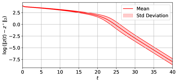
Figure 3: Mean (red curve) and standard deviation (shadow curve) of the lognorm of the Euclidean distance of 150 simulated trajectories of (40) with respect to the equilibrium point $z^{\star}$. In agreement with Theorem V.3 the convergence is linearly-exponentially bounded.

VI Conclusion

We analyzed the convergence characteristics of GW-LS-C dynamics, which naturally arise from convex optimization problems with a unique minimizer. For such dynamics, we showed linear-exponential convergence to the equilibrium. Specifically, we demonstrated that linear-exponential dependency arises naturally in certain dynamics with saturations and used this result for our convergence analysis. Depending on the norms where the system is GW-LS-C, we considered two different scenarios that required two distinct mathematical approaches, yielding convergence bounds that are sharper than those in [4]. Finally, after giving a sufficient condition for local ISS, we illustrated our results on the continuous-time augmented primal-dual dynamics solving LPs. Our results motivated a conjecture relating the optimal solution of LPs to the local stability properties of the equilibrium of the resulting dynamics. Our future work will include proving this conjecture, extending our ISS analysis to the case of different norms and further developing our results to design biologically plausible neural networks.

Appendix A Contraction times with respect to distinct norms

First we recall the following [4, Lemma V.1]

Lemma A.1 (Inclusion between balls computed with respect to different norms):

Given two norms $\|\cdot\|_{\alpha}$ and $\|\cdot\|_{\beta}$ on $\mathbb{R}^{n}$, for all $x\in\mathbb{R}^{n}$ and $r>0$, it holds

$$B{\bigl{(}x,r/k_{\alpha}^{\beta};\beta\bigr{)}}\subseteq B{\bigl{(}x,r;\alpha\bigr{)}}\subseteq B{\bigl{(}x,rk_{\beta}^{\alpha};\beta\bigr{)}}.$$ (43)

The following Lemma is inspired by [4, Theorem V.2]. For completeness, we here provide a self-contained proof.

Lemma A.2 (Contraction times with respect to distinct norms):

Given $\|\cdot\|_{\alpha}$ and $\|\cdot\|_{\beta}$ norms on $\mathbb{R}^{n}$ with equivalence ratio $k_{\alpha,\beta}$, consider system (4) satisfying Assumptions ($A$2), ($A$3) with $\|\cdot\|_{\textup{L}}=\|\cdot\|_{\alpha}$. Then, for each $0<\rho<1$,

1. the $\rho$-contraction time is $t_{\rho}=\ln(\rho^{-1})/c$;

2. the $\rho$-contraction time with respect to the norm $\|\cdot\|_{\beta}$ is $t_{\rho}^{\alpha,\beta}=\ln(k_{\alpha,\beta}\,\rho^{-1})/c$.

• Consider a trajectory $x(t)$ of system (4) such that $\|x_{0}\|_{\alpha}\leq{r}$. To prove (i) we need to find the first time $t_{\rho}$ such that $\|x(t_{\rho})-x^{\star}\|_{\alpha}\leq{\rho r}$. Clearly the worst-case time is achieved when $\|x_{0}-x^{\star}\|_{\alpha}={r}$. But $c$-strongly infinitesimal contractivity with respect to $\|\cdot\|_{\alpha}$ implies $\|x(t)-x^{\star}\|_{\alpha}\leq\mathrm{e}^{-ct}\|x_{0}-x^{\star}\|_{\alpha}$ and so $t_{\rho}$ is determined by the equality $\mathrm{e}^{-ct_{\rho}}r=\rho r$, from which item (i) follows.

  Regarding item (ii), we need to find the first time $t_{\rho}^{\alpha,\beta}$ such that $\|x(t_{\rho})-x^{\star}\|_{\beta}\leq{\rho r}$. We note that

  $$x_{0}\in B_{\beta}{\bigl{(}x^{\star},r\bigr{)}}\quad \overset{\eqref{ineq:balls:inclusions},\text{ $2^{\textup{nd}}$ inequality}}{\implies}\quad x_{0}\in B_{\alpha}{\bigl{(}x^{\star},k_{\alpha}^{\beta}r\bigr{)}},$$

  $$x(t_{\rho})\in B_{\beta}{\bigl{(}x^{\star},\rho r\bigr{)}}\quad \overset{\eqref{ineq:balls:inclusions},\text{ $1^{\textup{st}}$ inequality}}{\impliedby}\quad x(t_{\rho})\in B_{\alpha}{\bigl{(}x^{\star},\rho r/k_{\beta}^{\alpha}\bigr{)}}.$$

  Thus, the contraction time from $B_{\beta}{\bigl{(}x^{\star},r\bigr{)}}$ to $B_{\beta}{\bigl{(}x^{\star},\rho r\bigr{)}}$ is upper bounded by the contraction time from $B_{\alpha}{\bigl{(}x^{\star},k_{\alpha}^{\beta}r\bigr{)}}$ to $B_{\alpha}{\bigl{(}x^{\star},\rho r/k_{\beta}^{\alpha}\bigr{)}}$. Therefore, the contraction factor with respect to the $\|\cdot\|_{\alpha}$ norm is $(\rho r/k_{\beta}^{\alpha})/(k_{\alpha}^{\beta}r)=\rho/k_{\alpha,\beta}$. Item (ii) then follows from item (i). ∎

References

- [1] K. J. Arrow, L. Hurwicz, and H. Uzawa, editors. Studies in Linear and Nonlinear Programming. Stanford University Press, 1958.
- [2] G. Bianchin, J. Cortés, J. I. Poveda, and E. Dall’Anese. Time-varying optimization of LTI systems via projected primal-dual gradient flows. IEEE Transactions on Control of Network Systems, 9(1):474–486, 2022. doi:10.1109/TCNS.2021.3112762.
- [3] F. Bullo. Contraction Theory for Dynamical Systems. Kindle Direct Publishing, 1.1 edition, 2023, ISBN 979-8836646806. URL: https://fbullo.github.io/ctds.
- [4] V. Centorrino, A. Gokhale, A. Davydov, G. Russo, and F. Bullo. Positive competitive networks for sparse reconstruction. Neural Computation, January 2024. To appear. doi:10.48550/arXiv.2311.03821.
- [5] E. K. P. Chong, S. Hui, and S. H. Zak. An analysis of a class of neural networks for solving linear programming problems. IEEE Transactions on Automatic Control, 44(11):1995–2006, 1999. doi:10.1109/9.802909.
- [6] F. H. Clarke. Optimization and Nonsmooth Analysis. John Wiley & Sons, 1983, ISBN 047187504X.
- [7] S. Coogan. A contractive approach to separable Lyapunov functions for monotone systems. Automatica, 106:349–357, 2019. doi:10.1016/j.automatica.2019.05.001.
- [8] A. Davydov, V. Centorrino, A. Gokhale, G. Russo, and F. Bullo. Contracting dynamics for time-varying convex optimization. IEEE Transactions on Automatic Control, June 2023. Submitted. doi:10.48550/arXiv.2305.15595.
- [9] A. Davydov, A. V. Proskurnikov, and F. Bullo. Non-Euclidean contraction analysis of continuous-time neural networks. IEEE Transactions on Automatic Control, August 2023. Submitted. doi:10.48550/arXiv.2110.08298.
- [10] N. K. Dhingra, S. Z. Khong, and M. R. Jovanović. The proximal augmented Lagrangian method for nonsmooth composite optimization. IEEE Transactions on Automatic Control, 64(7):2861–2868, 2019. doi:10.1109/TAC.2018.2867589.
- [11] S. Hassan-Moghaddam and M. R. Jovanović. Proximal gradient flow and Douglas-Rachford splitting dynamics: Global exponential stability via integral quadratic constraints. Automatica, 123:109311, 2021. doi:10.1016/j.automatica.2020.109311.
- [12] S. Jafarpour, P. Cisneros-Velarde, and F. Bullo. Weak and semi-contraction for network systems and diffusively-coupled oscillators. IEEE Transactions on Automatic Control, 67(3):1285–1300, 2022. doi:10.1109/TAC.2021.3073096.
- [13] H. K. Khalil. Nonlinear Systems. Prentice Hall, 3 edition, 2002, ISBN 0130673897.
- [14] W. Lohmiller and J.-J. E. Slotine. On contraction analysis for non-linear systems. Automatica, 34(6):683–696, 1998. doi:10.1016/S0005-1098(98)00019-3.
- [15] H. D. Nguyen, T. L. Vu, K. Turitsyn, and J.-J. E. Slotine. Contraction and robustness of continuous time primal-dual dynamics. IEEE Control Systems Letters, 2(4):755–760, 2018. doi:10.1109/LCSYS.2018.2847408.
- [16] G. Russo, M. Di Bernardo, and E. D. Sontag. Global entrainment of transcriptional systems to periodic inputs. PLoS Computational Biology, 6(4):e1000739, 2010. doi:10.1371/journal.pcbi.1000739.
- [17] D. W. Tank and J. J. Hopfield. Simple ”neural” optimization networks: An A/D converter, signal decision circuit, and a linear programming circuit. IEEE Transactions on Circuits and Systems, 33(5):533–541, 1986. doi:10.1109/TCS.1986.1085953.
- [18] S. Xie, G. Russo, and R. H. Middleton. Scalability in nonlinear network systems affected by delays and disturbances. IEEE Transactions on Control of Network Systems, 8(3):1128–1138, 2021. doi:10.1109/TCNS.2021.3058934.