Logarithmic critical slowing down in complex systems: from statics to dynamics

Abstract

We consider second-order phase transitions in which the order parameter is a replicated overlap matrix. We focus on a tricritical point that occurs in a variety of mean-field models and that, more generically, describes higher order liquid-liquid or liquid-glass transitions. We show that the static replicated theory implies slowing down with a logarithmic decay in time. The dynamical equations turn out to be those predicted by schematic Mode Coupling Theory for supercooled viscous liquids at a $A_{3}$ singularity, where the parameter exponent is $\lambda=1$. We obtain a quantitative expression for the parameter $\mu$ of the logarithmic decay in terms of cumulants of the overlap, which are physically observable in experiments or numerical simulations.

I Introduction

In the present work we study a peculiar kind of critical slowing down occurring in the dynamics of slowly relaxing complex glassy systems, in which the correlation function of the relevant dynamic variables decays logarithmically in time. This is different from the usual behavior of, e. g., the correlation function of density fluctuations in supercooled liquid next to the dynamic arrest occurring in mean-field theories for glasses, somehow describing the real-world (off-equilibrium) glass transition of liquid glass-formers. In that case, the correlator next to the transition displays a two step behavior: towards a plateau at short times and from the plateau towards zero correlation at longer times. The plateau becoming longer and longer as the external parameters bring the system nearer to the dynamic arrest line in the phase diagram. In Götze’s Mode-Coupling Theory (MCT) Götze (1984, 1985, 1991, 2009) a dynamic arrest critical point is referred to as a $A_{2}$ singularity, according to the classification of Arnold’s catastrophes theory. The critical point corresponding to a logarithmic decay is, instead, a $A_{3}$ cusp singularity, a tricritical point signalling the end-point of a liquid-liquid (or glass-glass) dynamic transition.

More in detail, the behavior in time of the correlation function $C(t)$ in the time-translational invariant (TTI) regime at the ground of MCT is usually characterized by an initial power-law decay $t^{-a}$ towards a constant value, often related to the $\beta$ relaxation occurring in glass formers, and by a decay $-t^{b}$ from the plateau of $C(t)$ as the liquid system begins approaching thermodynamic equilibrium. The exponents $a$ and $b$ are related by the well known formula for the so-called “parameter exponent”

$$\lambda={\Gamma^{2}(1-a)\over\Gamma(1-2a)}={\Gamma^{2}(1+b)\over\Gamma(1+2b)}\ ,$$ (1)

holding at the dynamical $A_{2}$ singularity of the MCT for undercooled viscous liquids. Changing the values of the external parameters a dynamic arrest line can be drawn in the phase diagram consisting of $A_{2}$ points. In given systems the exponent parameter $\lambda$ tends to $1$ along the dynamic arrest line, approaching a $A_{3}$ point. In that limit the exponent $a$ tends to zero and logarithmic corrections become relevant to the relaxation.

Hereafter, we present a general method for the quantitative computation of the coefficient of the logarithmic decay of the density-density correlation functions in viscous liquids. Göetze and Sjögren Gotze and Sjogren (1989) predicted a $1/\ln t^{2}$ decay exactly at the $A_{3}$ singularity and a behavior of the kind $-(\ln t)^{\gamma}$ as $a\sim 0$, $\lambda\sim 1$. Their exemplifying case is the $F_{13}$ mode-coupling schematic theory. However, in this case, the $A_{3}$ singularity cannot be directly accessed in experiments or in numerical simulations because it occurs in the region of the phase diagram pertaining to the glassy phase, beyond the dynamic arrest line where TTI breaks down and the MCT does not hold anymore. Therefore, in the liquid phase the presence of the $A_{3}$ singularity is only felt in weakly logarithmic corrections to the power-law $\beta$ decay in regions of the space parameters (temperature, packing fraction, …) close enough to it. Other systems displaying this kind of singularity include disordered spin-glass models Crisanti et al. (1993a); Crisanti and Leuzzi (2006, 2015); Franz et al. (2013); Cammarota and Biroli (2012a), liquids in porous media both in the MCT Krakoviack (2005, 2007) and in the HNC approximations Madden and Glandt (1988); Given and Stell (1992) and liquid models with pinned particles Cammarota and Biroli (2012b). The $-\ln t$ behavior of the correlation function appears to be the correct fitting law for about a decade or two in most of the known experiments and numerical simulations of repulsive colloids Sjogren (1991); Zaccarelli et al. (2002); Sciortino et al. (2003a, b); Götze (2009). Also cases where the $A_{3}$ singularity is directly accessible from the liquid phase are devised in MCT, for instance in the $F_{12}$ schematic model. The quantitative estimation of the parameters of the logarithmic behavior can, so far, be performed exactly only in MCT schematic theories. Moreover, as, e.g., in the case of the $F_{13}$ model, the $A_{3}$ singularities lie in the region where one of the fundamental assumptions on which MCT is built, TTI, does not hold.

In many systems the replica method offers a way to characterize dynamical arrest phenomena in a purely static framework which is often simpler than a dynamical approach. It is, therefore, natural to assume that universal static critical properties can be obtained a la Landau from simple assumptions on the (replicated) Gibbs free energy at the corresponding critical point. A decade ago, it was realized that replicated theories also determine important features of critical glassy dynamics Caltagirone et al. (2012a, b, c); Ferrari et al. (2012); Parisi and Rizzo (2013a). Notably, they give the same scale-invariant equations for the critical correlators that are often obtained by studying the actual dynamical equations of these systems. An important consequence is that the exponent parameter $\lambda$, Eq. (1), can be computed in a static replicated theory.

In this paper we consider a class of replicated theories for which $\lambda=1$ and show that they predict a logarithmic decay of the correlation as obtained within MCT at the $A_{3}$ singularity. Furthermore, we show that the coefficient describing the logarithmic decay can be quantitatively expressed in terms of static quantities that can be measured at equilibrium and we provide the formula (18), which is the most notable result of the present work.

The paper is organized as follows. In section II we present the general framework and the results. In section III we derive the equations for critical dynamics starting from the replicated theory. In section IV we report the general expansion of the free energy. In section V we connect the free energy with the Gibbs free energy and we derive the main results. In section VI we give our conclusions. In appendix A we report the $23$ fourth order vertices, as well as their associated cumulants combinations.

II Outline of the Results

The framework of this paper is a Landau approach to glassiness based on replicated theories. In a Landau approach one does not start from any specific microscopic model, and instead: (i) identifies an order parameter, (ii) makes some assumptions on the structure of the corresponding Gibbs free energy near a critical point and (iii) explores the consequences of these assumptions. The corresponding results display a great deal of universality because the assumptions of the structure of the Gibbs free energy can be valid for many different models, often with completely different microscopic structures. On the other hand, to be concrete, one can usually exhibit solvable mean-field models whose Gibbs free energy, as given by a first principles computation, has precisely the required structure. Solvable models are typically obtained considering either long-range models or taking the limit of infinite dimensions, later on in this section we will mention a few mean-field models to which our general findings apply.

We will follow and expand the derivation of Ref. Parisi and Rizzo (2013a), considering theories in which the argument of the Gibbs free energy $G(Q)$ is a replicated matrix $Q_{ab}$ with $a=1,\dots,n$. The replica number $n$ in these theories is usually continued from integer to real continuous values, and we will take into account the two important cases $n\rightarrow 0$ and $n\rightarrow 1$. Such $Q_{ab}$ matrix naturally appears in Spin-Glasses where, due to the presence of quenched disorder, one resorts for technical reasons to the replica method. From a physical point of view, the order parameter to identify a glassy phase, i.e., a ”multi-equilibria” phase composed by many different states, cannot rely on an absolute reference for a state, since no a priori clear pattern is provided because of frustration. As a consequence, the order parameter is built on the similarity between different states. More precisely, on the whole range (hierarchy) of possible similarities, summed up in a probability distribution for the values of the overlap matrix elements. In this case $Q_{ab}$ is naturally identified with the average of the overlap between two different replicas of the system

$$Q_{ab}={1\over N}\sum_{i=1}^{N}\overline{\langle s_{i}^{a}s_{i}^{b}\rangle}\ .$$ (2)

For the case $n\to 0$ the angle brackets are thermal averages and the overline is the average over the quenched disorder. The case $n\to 1$ applies to problems where for each disorder realization there are many metastable excited states, whose number grows exponentially with the size of the system. In this latter case, then, the angle brackets represent thermal averages inside a metastable state and the overline represents averages over different metastable states and over the quenched disorder.

It has been argued that a replicated order parameter may be the relevant one whenever the frozen state is amorphous because to detect symmetry-breaking we have to compare it with itself. This has led to the extension of the replica method to structural glasses Mézard and Parisi (1996, 1999a); Mézard (1999); Mézard and Parisi (1999b, 2000) and more recently to the development of the theory of supercooled liquids in the limit of infinite dimensions Parisi et al. (2020). In this context $Q_{ab}$ is naturally identified with the averaged density-density fluctuations in the momentum space in a replicated system at some wave vector $\bm{k}$:

$$Q_{ab}\equiv{1\over V}{\langle\delta\rho^{*}_{a}(\bm{k})\delta\rho_{b}(\bm{k})\rangle}.$$ (3)

where $\rho_{a}(k)$ is the Fourier transform

$$\rho_{a}(\bm{k})=\sum_{i=1}^{N}e^{\imath\,\bm{k}\cdot\bm{r}_{i}^{(a)}}$$

of the density of $N$ particles of the replica $a$ at positions $r_{i,a}$, $i=1,\ldots,N$,

$$\rho(\bm{r}^{(a)})=\sum_{i=1}^{N}\delta\left(\bm{r}^{(a)}-\bm{r}_{i}^{(a)}\right)$$

and $\delta\rho_{a}(\bm{k})$ is the fluctuation of $\rho_{a}(\bm{k})$ with respect to its average $\langle\rho_{a}(\bm{k})\rangle$. We note that choice of $\bm{k}$ in Eq. (3) is free arbitrary and one could consider, instead, the mean-square-displacement Parisi et al. (2020). We refer the reader to section II.B of Rizzo (2016) for a thorough discussion on the choice of the order parameter.

In mean-field models we expect that the Gibbs free energy has a regular expansion in powers of the order parameter at the critical point, therefore we will consider the following Replica-Symmetric theory written in terms of $\delta Q_{ab}\equiv Q_{ab}-Q_{c}$ where $Q_{c}$ is the value of the order parameter at the critical point and $\delta Q_{aa}=0$:

$$G(\delta Q) = \frac{m_{1}}{2}\sum_{ab}^{1,n}\delta Q_{ab}^{2}+\frac{m_{2}}{2}\sum_{abc}^{1,n}\delta Q_{ab}\delta Q_{ac}$$

$$+ \frac{m_{3}}{2}\sum_{abcd}^{1,n}\delta Q_{ab}\delta Q_{cd}$$

$$- {w_{1}\over 6}{\rm Tr}\,\delta Q^{3}-{w_{2}\over 6}\sum_{ab}^{1,n}\delta Q_{ab}^{3}$$

$$- {1\over 24}\Bigl{[}y_{1}{\rm Tr}\,\delta Q^{4}+y_{2}\sum_{ab}^{1,n}\delta Q_{ab}^{4}$$

$${\color[rgb]{0,0,0}{+y_{3}\sum_{abc}^{1,n}\delta Q_{ab}^{2}\delta Q_{ac}^{2}}}+y_{4}\sum_{abc}^{1,n}\delta Q_{ab}^{2}\delta Q_{ac}\delta Q_{cb}\Bigr{]}\ .$$

The above expression can be obtained from a microscopic description in a variety of contexts Mézard et al. (1987); Parisi et al. (2020). In the above expression we have retained only the terms relevant for the present discussion (the $y_{3}$ term, actually, vanishes, as will be shown in Sec. III.1), while the complete expression has actually eight third-order terms and twenty-three fourth-order terms that will be displayed later, in appendix A. At the end of section IV we will explain why the other terms can be neglected. We will focus on critical points characterized by the condition $m_{1}=0$. Depending on the values of the remaining parameters and on the replica number $n$ we may have different types of transition. Three such transitions, discussed in detail in Parisi and Rizzo (2013a) are:

• $m_{2}=m_{3}=0$ and replica number $n\to 0$, that corresponds to a standard Spin-Glass (SG) transition in zero field or to the so-called degenerate $A_{2}$ singularity within MCT,

• $m_{2}\neq 0\neq m_{3}$ and replica number $n\to 0$, that corresponds to the SG transition in a field that occurs along the de Almeida-Thouless line Mézard et al. (1987); Crisanti et al. (1993b), and

• $m_{2}\neq 0\neq m_{3}$ and replica number $n\to 1$ that corresponds to the dynamical transition in SG systems that is the well-known $A_{2}$ singularity in MCT Franz et al. (2011); Rizzo (2016).

In dynamics one is typically interested in the correlation $C(t)$ between the configuration of the system at time $t=0$ and the configuration of the system at time $t$ which is the dynamical counterpart of the two-point order parameter $Q_{ab}$. In spin systems it is naturally defined as:

$$C(t)\equiv{1\over N}\sum_{i=1}^{N}\overline{\langle s_{i}(0)s_{i}(t)\rangle}$$ (5)

while in structural glasses it is given by

$$C(t)\equiv{1\over V}{\langle\delta\rho^{*}(\bm{k},0)\ \delta\rho(\bm{k},t)\rangle}$$ (6)

In the liquid/paramagnetic phase the function $C(t)$ decays exponentially but the correlation time diverges at the critical point. As mentioned in the introduction it has been shown Parisi and Rizzo (2013a) that the structure of the replicated Gibbs free energy at the critical point determines also the essential features of critical dynamics. More precisely in the case of the SG transition (i) one can show that the TTI correlation at large time-differences $t$ is described by:

$$C(t)=m_{1}\,f\left(\frac{t}{t^{*}}\right)\ \ \ t\gg 1,\$$ (7)

for small positive $m_{1}$, where the time scale $t^{*}$ grows like

$$t^{*}\propto{1\over m_{1}^{1\over a}},$$

the exponent $a$ is a solution of the equation

$${w_{2}\over w_{1}}={\Gamma^{2}(1-a)\over\Gamma(1-2a)}\ ,$$ (8)

and the function $f(x)$ obeys the scale invariant equation:

$$0\, = \,f(x)\,+f^{2}(x)\left(1-{w_{2}\over w_{1}}\right)$$

$$+\int_{0}^{x}\left[f(x-y)-f(x)\right]\dot{f}(y)dy.$$

The solution of the above equation diverges as $1/x^{a}$ for $x\rightarrow 0$ and goes exponentially to zero for $x\rightarrow\infty$. Precisely at $m_{1}=0$ the correlation undergoes critical slowing down and decays as a power law with exponent $a$, rather than as an exponential. Similar results are obtained for transitions (ii) and (iii), as, e.g., for the SK model in a field, the $p$-spin spherical and Ising models, the Random Orthogonal model, or the Potts model Caltagirone et al. (2012a); Ferrari et al. (2012); Caltagirone et al. (2012b, c). In particular, for the transition of type (iii) one recovers exactly the same scale invariant equations of the critical correlators in MCT (i.e. eq. 6.55a in Götze (2009)) with the parameter exponent given by:

$$\lambda={w_{2}\over w_{1}},$$ (10)

The above results show that critical dynamics at the three transitions considered is universal because it follows solely from the structure of the replicated Gibbs free energy. Furthermore the above relationship extends the range of predictions that the replica approach can provide. Besides, the connection between the replicated Gibbs free energy and the parameter exponent leads to a connection with connected correlation functions of the order parameter: the proper vertexes $w_{2}$ and $w_{1}$ in Eq. (II) are associated to vertexes of the Free energy, function of fields in the replica space coupled to the overlap fluctuations, which are given by the connected correlation functions of $\delta Q_{ab}$. For instance, one obtains that

$${w_{2}\over w_{1}}={\omega_{2}\over\omega_{1}}$$ (11)

where $\omega_{1}$, $\omega_{2}$ are six-point functions given, respectively, by:

$$\omega_{1}={1\over N}\sum_{ijk}\overline{\langle s_{i}s_{j}\rangle_{c}\langle s_{j}s_{k}\rangle_{c}\langle s_{k}s_{i}\rangle_{c}}$$ (12)

$$\omega_{2}={1\over 2N}\sum_{ijk}\overline{\langle s_{i}s_{j}s_{k}\rangle_{c}^{2}}\ ,$$ (13)

where the suffix $c$ stands for connected correlation functions. As mentioned before, we recall that for transition (i) and (ii) ($n\to 0$) the angle brackets in the above expressions stand for thermal averages and the overline stands for the average over the quenched disorder. For transition (iii) ($n\to 1$) the angle brackets in the above expression stand for thermal averages inside a metastable state and the overline stands for the average over the different metastable states and over the quenched disorder.

In this paper we extend the above analysis to a class of critical points characterized by a replicated Gibbs free energy of the type (II) but with $w_{2}=w_{1}\equiv w$, i. e., with $\lambda=1$. To be definite let us give a few examples of solvable mean-field models that display such a transition. Let us consider the most general fully connected Spin-Glass models with multi-$p$-spin interactions:

$$\mathcal{H}=-\sum_{p}\,\sum_{i_{1}<i_{2}<\dots<i_{p}}J_{i_{1}\dots i_{p}}s_{i_{1}}\dots s_{i_{p}}$$ (14)

where the $J^{\prime}s$ are quenched random interactions and the $s_{i}$ can be either Ising spin or satisfy a spherical constraint. In the spherical $3$-spin case in presence of a magnetic field there is a tricritical point with $\lambda=1$ in the temperature-magnetic field plane where a line of discontinuous transitions meets a line of continuous transitions Crisanti and Sommers (1992); Crisanti et al. (1993a). Another example is that of a mixed $2+3$ model that corresponds to the so-called schematic $F_{12}$ model in the context of MCT. In the phase diagram, e.g., in the plane of the magnitudes of the $2$-spin and the $3$-spin interaction there is a $\lambda=1$ critical point. Upon increasing the relative magnitude of the $3$-spin interaction, a line of continuous transitions meets a line of discontinuous transitions Franz et al. (2013); Caltagirone et al. (2013). Random pinning of a spherical $p$-spin glass model, i.e. freezing a fraction $c$ of the spins Cammarota and Biroli (2012b, a), is also relevant: in the temperature-concentration plane there is a line of discontinuous transitions that, upon increasing the concentration, ends in a point characterized by $\lambda=1$. Finally we mention the Potts Spin-Glass with Hamiltonian:

$$\mathcal{H}=-\sum_{i<j}\,J_{ij}\,(p\,\delta_{s_{i}s_{j}}-1)$$ (15)

where the $s_{i}$ are Potts spins with $p$ states and $J_{ij}$ is a quenched random interaction. For $p\leq 4$ it displays a continuous SG transition characterized by $\lambda=(p-2)/2$, which implies $\lambda=1$ for $p=4$, in both the fully connected Gross et al. (1985); Caltagirone et al. (2012c) and the finite-connectivity case Goldschmidt (1988).

If $\lambda=1$ the correlation cannot decay with a power-law because eqs. (10) or (1) yield $a=b=0$. Indeed for all the three types of transitions we will show that, at large times:

$$C(t)-C(\infty)=\ {2\pi^{2}\over 3\,\mu\ln^{2}(t/t_{1})}+{24\zeta(3)\over\mu\ln^{3}(t/t_{1})}\ln\ln(t/t_{1})+\dots$$ (16)

where $\zeta(i)$ is the Riemann’s $\zeta$-function and $t_{1}$ is an unkwown time scale that cannot be determined due to the time-scale invariance of equation. We note that this expression was obtained by Götze and Sjögren Gotze and Sjogren (1989) within MCT in the context of the so-called $A_{3}$ singularities Götze (2009) and, indeed, we will derive the same dynamical equations. The parameter $\mu$ in Eq. (16) depends on the quartic coupling constants of the Replicated Gibbs Free energy (II) through:

$$\mu=-{y_{1}+y_{2}-y_{4}\over 3w}\ .$$ (17)

As usual, the coefficients of the Gibbs free energy can be expressed in terms of four-point connected correlation functions of the order parameter and, thus, we will show that the parameter $\mu$ can be calculated in terms of physical measurable observables as

$$\mu=-\frac{r}{3\omega}\left(\upsilon_{1}+\upsilon_{2}-\upsilon_{4}\right)$$ (18)

where $r\equiv\chi_{SG}^{-1}$, $\chi_{SG}$ being the so-called Spin-Glass susceptibility:

$$\chi_{SG}\equiv{1\over N}\sum_{ij}\overline{\langle s_{i}s_{j}\rangle^{2}_{c}}\ ,$$ (19)

whereas $\omega$ is either given by $\omega_{1}$ or $\omega_{2}$ defined in Eqs. (12,13) since they are equal at the critical point that we are considering. Eventually, the $\upsilon$’s are the fourth-order analogs of the $\omega$’s. As we will show in Sec. IV, their expressions turn out to be:

$$\upsilon_{1} \equiv {3\over N}\sum_{ijkl}\overline{\langle s_{i}s_{j}\rangle_{c}\langle s_{j}s_{k}\rangle_{c}\langle s_{k}s_{l}\rangle_{c}\langle s_{l}s_{i}\rangle_{c}}$$ (20)

$$\upsilon_{2} \equiv {1\over 2N}\sum_{ijkl}\overline{\langle s_{i}s_{j}s_{k}s_{l}\rangle_{c}^{2}}$$ (21)

$$\upsilon_{4} \equiv {6\over N}\sum_{ijk}\overline{\langle s_{i}s_{j}s_{k}\rangle_{c}\langle s_{i}s_{j}s_{l}\rangle_{c}\langle s_{l}s_{k}\rangle_{c}}$$ (22)

We will also consider the critical behavior of the physical susceptibilities. In particular, we will show that close to the critical point, where $r$ vanishes linearly with the external parameters (in mean-field models), the three-point susceptibilities $\omega_{i}$, $i=1,2$, diverge as

$$\omega_{i}=\frac{w_{i}}{r^{3}}$$ (23)

and the four-point susceptibilities $\upsilon_{i}$, $i=1,\dots,4$, diverge as

$$\upsilon_{i}=O\left(\frac{1}{r^{5}}\right)\ .$$ (24)

However, the linear combination $\upsilon_{1}+\upsilon_{2}-\upsilon_{4}$ associated to $\mu$ is less divergent if $w_{1}=w_{2}$, as it turns out to obey the following relationship:

$$\upsilon_{1}+\upsilon_{2}-\upsilon_{4}=6\ \frac{(w_{1}-w_{2})^{2}}{r^{5}}+\frac{y_{1}+y_{2}-y_{4}}{r^{4}}$$ (25)

Equations (16), (17), (18) and (25) are the main results of this paper and will be derived in the following. In particular, Eqs. (16) and (17) will be derived in the following section. In section IV the free energy will be introduced, and the expression of its coefficients (20-22) will be derived. Eventually, Eq. (18) will be derived in section V.

III Derivation of the Equations of Critical Dynamics

In this section we show how the expression (16) can be derived from the static replicated Gibbs free energy (II). We first differentiate it with respect to the order parameter $\delta Q_{ab}$ obtaining the following equation of state:

$$0 = w_{1}(\delta Q^{2})_{ab}+w_{2}\delta Q^{2}_{ab}$$

$$+ {y_{1}\over 3}(\delta Q^{3})_{ab}+{y_{2}\over 3}\delta Q^{3}_{ab}$$

$$+ {\color[rgb]{0,0,0}{{y_{3}\over 6}\delta Q_{ab}\left[(\delta Q^{2})_{aa}+(\delta Q^{2})_{bb}\right]+}}{y_{4}\over 6}\delta Q_{ab}(\delta Q^{2})_{ab}$$

$$+ {y_{4}\over 12}\sum_{c}\left[\delta Q_{ac}^{2}\delta Q_{cb}+\delta Q_{bc}^{2}\delta Q_{ca}\right]$$

Now we translate the above equation into an equation for the dynamical correlation valid at large times and near the critical point. We will briefly sketch the arguments leading to this mapping but we refer the reader to Ref. Parisi and Rizzo (2013a) for all the details of the procedure. The result is obtained in the context of a super-field formulation of dynamics Kurchan (1992) in which both the dynamical correlation and response functions are represented by a single dynamical order parameter $Q(1,2)$ in terms of (commuting) times $t_{1,2}$ and Grassmannian anticommuting variables $\theta_{1,2}$, $\bar{\theta}_{1,2}$.

III.1 Theories with $n=0$

At equilibrium $Q(1,2)$ can be parameterized by a single time translational invariant correlation function $C(t)=C(-t)$ according to the following form that encodes causality and the Fluctuation-Dissipation-Theorem (FDT):

$$Q(1,2)=\left\{1+\Theta_{12}{\partial\over\partial t_{1}}\right\}C(t_{1}-t_{2})$$ (27)

with

$$\Theta_{12} \equiv {1\over 2}(\overline{\theta}_{1}-\overline{\theta}_{2})\left[\theta_{1}+\theta_{2}-(\theta_{1}-\theta_{2})\ {\rm sign}(t_{1}-t_{2})\right]$$ (31)

$$= \left\{\begin{array}[]{c c}(\bar{\theta}_{1}-\bar{\theta}_{2})\theta_{2}&,\quad t_{1}>t_{2}\\ &\vspace*{-.2cm}\hfil\\ (\bar{\theta}_{1}-\bar{\theta}_{2})\theta_{1}&,\quad t_{2}>t_{1}.\end{array}\right.$$

We note that this representation is appropriate for the phase transitions characterized by a replicated free energy with $n=0$, whereas for $n=1$ a different representation must be considered (Parisi and Rizzo (2013a), Sec. III.D). We postpone the discussion of this case to the end of this section. On general grounds it is to be expected that the dynamical order parameter $Q(1,2)$ at large times must be related to the static order parameter $Q_{ab}$. Indeed, as noted in Kurchan (1992), the static result is obtained in the so-called Fast Motion (FM) limit that corresponds to an infinitely fast microscopic dynamics. In this limit, configurations at different times are completely uncorrelated and they are equivalent to different replicas of the same system. As a consequence, in this limit $Q_{FM}(1,2)$ has a diagonal structure:

$$Q_{FM}(1,2)=\delta(1,2)\left[C(0)-C(\infty)\right]+C(\infty)\ ,$$ (32)

where $\delta(1,2)$ is a delta function in the super-variables and $C(0)$, $C(\infty)$ are the values of the correlation at zero and infinite time, respectively. It is useful to describe the dynamics at large but not infinite times in terms of the deviation of $Q(1,2)$ from its FM limit introducing the quantity

$$\delta Q(1,2)=Q(1,2)-Q_{FM}(1,2)\ .$$ (33)

The dynamical equations for $Q(1,2)$ can be obtained from a dynamical Gibbs free energy and one may expect that the critical dynamics is determined a la Landau by its expansion in powers of $\delta Q(1,2)$. In Parisi and Rizzo (2013a) it is argued that the dynamical Gibbs free energy must have the same structure of the replicated Gibbs free energy with the same coupling constants and, therefore, Eq. (III) translates into an identical equation for $\delta Q(1,2)$.

In the following we will rewrite Eq. (III) with $\delta Q_{ab}\rightarrow\delta Q(1,2)$ as an equation for $C(t)$. In order to simplify the computation we observe that all the terms are obtained from $\delta Q(1,2)$ through the operation of exponentiation of matrix elements and dot products. These operations preserve supersymmetry, time reversal, zero ghost number and causality (see Kurchan (1992), section 5.5) and, therefore, their result can still be written in the form (27) which is the most general form satisfying these properties. Using an appropriate even function $A(\tau)$, the generic exponentiation corresponds to a simple power:

$$A(1,2)^{k}=\left\{1+\Theta_{12}{\partial\over\partial t_{1}}\right\}A^{k}(t_{1}-t_{2})$$ (34)

The dot product corresponds to:

$$\int A(1,3)B(3,2)\ d3=\left\{1+\Theta_{12}{\partial\over\partial t_{1}}\right\}[AB](t_{1}-t_{2})$$ (35)

where the function $[AB](t)$ stands for:

$$[AB](t) = A(t)B(0)+B(t)A(0)$$

$$-A(\infty)B(-\infty)-{d\over dt}\int_{0}^{t}A(t-y)B(y)dy.$$

One can check that if both $A(t)$ and $B(t)$ are even functions, then $[AB](t)$ is even and $[AB](t)=[BA](t)$. We recall that $\delta Q(1,2)$ is also of the form (27) with $\delta C(t)=C(t)-C_{FM}(t)$ where $C_{FM}(t)$ obeys $C_{FM}(0)=C(0)$ and $C_{FM}(0^{+})=C(\infty)$. Therefore, by construction we have that $\delta C(0)=\delta C(\infty)=0$ and this simplifies considerably the evaluation of the various terms. Using the two rules $(\ref{Aprod})$ and $(\ref{AB12})$ we can translate all the terms of Eq. III into expressions of their dynamical counterparts. For the quadratic terms we have:

$$w_{1}(\delta Q^{2})_{ab} \rightarrow -w_{1}\ {d\over dt}\int_{0}^{t}\delta C(t-y)\ \delta C(y)\ dy$$ (37)

$$w_{2}\ \delta Q^{2}_{ab} \rightarrow w_{2}\ \delta C^{2}(t).$$ (38)

In order to make contact with the MCT notation of reference Gotze and Sjogren (1989) we define:

$$\delta C(t)\equiv G(t)$$ (39)

and introduce the Laplace transform of the time functions as Götze (2009):

$$\hat{A}(z)=LT[A(t)](z)\equiv i\int_{0}^{\infty}A(t)\ e^{izt}dt\qquad,\quad\mbox{Im}[z]>0.$$ (40)

The formulas for the transforms of the convolution and of the time derivative are repeatedly used in the following derivation and we write them explicitly

$$LT\left[\int_{0}^{t}A(t-y)B(y)dy\right]=-i\hat{A}(z)\hat{B}(z)$$ (41)

$$LT\left[{dA(t)\over dt}\right]=-iz\hat{A}(z).$$ (42)

We also define $(G^{2})(t)$ as the time derivative of the convolution, cf. Eq. (III.1):

$$(G^{2})(t)\equiv-{d\over dt}\int_{0}^{t}G(t-y)\ G(y)\ dy\ .$$ (43)

The contributions of the quadratic terms can now be expressed as:

$$w_{1}\ (\delta Q^{2})_{ab} \rightarrow w_{1}\ z\ \hat{G}^{2}(z)\ ,$$ (44)

$$w_{2}\ \delta Q^{2}_{ab} \rightarrow w_{2}\ LT[G^{2}(t)]\ ,$$ (45)

while those of the cubic terms can be expressed as:

$${y_{1}\over 3}\ (\delta Q^{3})_{ab} \rightarrow {y_{1}\over 3}\ z^{2}\hat{G}^{3}(z)$$ (46)

$${y_{2}\over 3}\ \delta Q^{3}_{ab} \rightarrow {y_{2}\over 3}\ LT[G^{3}(t)]$$ (47)

$${y_{3}\over 6}\ \delta Q_{ab}((\delta Q^{2})_{aa}+(\delta Q^{2})_{bb}) \rightarrow 0$$ (48)

$${y_{4}\over 6}\ \delta Q_{ab}(\delta Q^{2})_{ab} \rightarrow {y_{4}\over 6}\ LT[G(t)(G^{2})(t)]$$ (49)

$${y_{4}\over 12}\ \sum_{c}[\delta Q_{ac}^{2}\delta Q_{cb}+\delta Q_{bc}^{2}\delta Q_{ca}] \rightarrow {y_{4}\over 6}\ z\ \hat{G}(z)\ LT[G^{2}(t)].$$ (50)

We stress that, in order to compute the vanishing term proportional to $y_{3}$, we have used the fact that, according to Eqs. (35) and (III.1):

$$AB(1,1)=[AB](0)=A(0)B(0)-A(\infty)B(-\infty)\ ,$$ (51)

that implies:

$$(\delta Q^{2})_{aa}\rightarrow\delta C(0)^{2}-\delta C^{2}(\infty)=0\ .$$ (52)

Dividing Eq. (III) by $w_{1}$ and multiplying by $z$, we obtain:

$$0 = z\left\{{w_{2}\over w_{1}}LT[G^{2}(t)]+z\ \hat{G}^{2}(z)\right\}$$ (53)

$$+ {y_{1}+y_{2}-y_{4}\over 3w_{1}}\ z\ LT[G^{3}(t)]$$

$$- {2y_{1}-y_{4}\over 6w_{1}}\ z\left\{LT[G^{3}(t)]-z^{2}\hat{G}^{3}(z)\right\}$$

$$+ {y_{4}\over 6w_{1}}\ z\ \left\{LT[G^{3}(t)]+z\ \hat{G}(z)\ LT[G^{2}(t)]\right\}$$

$$+ {y_{4}\over 6w_{1}}\ z\ \left\{LT[G(t)(G^{2})(t)]+z^{2}\ \hat{G}^{3}(z)\right\},$$

where we have just rearranged the various term for later convenience. Shortening $\mu\equiv(y_{1}+y_{2}-y_{4})/(3w_{1})$, the first two lines correspond to the equation

$$0 = z\left\{{w_{2}\over w_{1}}LT[G^{2}(t)]+z\ \hat{G}^{2}(z)\right\}-\mu\ z\ LT[G^{3}(t)]$$ (54)

considered by Göetze and Sjögren Gotze and Sjogren (1989) who showed that its solution at leading order follows the logarithmic decay of Eq. (16). Our equation (53) has the same form except for the additional terms of the last three lines. In order to characterize its solution one introduces an auxiliary function $g$ by setting $G(t)=g(\ln(t/t_{1}))$. Following Gotze and Sjogren (1989) we introduce the variable

$$y\equiv\ln\frac{1}{-izt_{1}}$$

and, changing the integration variable in the Laplace transform from $t$ to $u\equiv-izt$, we obtain the relationship

$$-z\,\ \ {\hat{G}}(z)=\int_{0}^{\infty}\,du\,e^{-u}g(y+\ln\,u).$$ (55)

The Taylor expansion around $y$ gives:

$$-z\,\hat{G}(z)=g(y)+\Gamma_{1}\ g^{\prime}(y)+{1\over 2}\Gamma_{2}\,\ g^{\prime\prime}(y)+\dots$$ (56)

where

$$\Gamma_{n}\equiv\int_{0}^{\infty}du\,e^{-u}(\ln u)^{n}\ .$$ (57)

It follows that for a generic product the Laplace transforms reads

$$-z\,LT[G_{1}^{p}(t)G_{2}^{q}(t)](z) = g_{1}^{p}g_{2}^{q}+\Gamma_{1}(pg_{1}^{\prime}g_{1}^{p-1}g_{2}^{q}+qg_{2}^{\prime}g_{2}^{q-1}g_{1}^{p})+$$ (58)

$$+ {1\over 2}\Gamma_{2}\,(\,p(p-1)g_{1}^{\prime\prime}\,g_{1}^{p-2}g_{2}^{q}\ +pqg_{1}^{\prime}g_{2}^{\prime}\,g_{1}^{p-1}g_{2}^{q-1}\ +q(q-1)g_{2}^{\prime\prime}\,g_{2}^{q-2}g_{1}^{p})+\dots$$

The integrals $\Gamma_{n}$ can be expressed as polynomials of degree $n$ of the Euler’s constant $\gamma=-\Gamma_{1}$, with coefficients given by combinations of the Riemann’s zeta function up to $\zeta(n)$. Furthermore, given any two functions $G_{1}(t)$ and $G_{2}(t)$ and the corresponding functions $g_{1}$ and $g_{2}$ we have :

$$-z\left\{LT\left[G_{1}(t)G_{2}(t)\right]+z\ \hat{G}_{1}(z)\ \hat{G}_{2}(z)\right\}=\zeta(2)g_{1}^{\prime}g_{2}^{\prime}+\dots\ ,$$ (59)

where $\zeta(2)={\pi^{2}/6}$. With the help of the above formulas we obtain:

$$z\big{\{}LT[G^{2}(t)]+z\ \hat{G}^{2}(z)\big{\}} = -\zeta(2)(g^{\prime})^{2}+2(\gamma\zeta(2)+\zeta(3))g^{\prime}g^{\prime\prime}+\dots$$

$$zLT[G^{3}(t)] = -g^{3}+3\gamma g^{2}g^{\prime}+\dots$$

$$z\{LT[G^{3}(t)]-z^{2}\ \hat{G}^{3}(z)\} = O\left(g\ (g^{\prime})^{2}\right)$$

$$z\{LT[G^{3}(t)]+z\ \hat{G}(z)\ LT[G^{2}(t)]\} = O\left(g\ (g^{\prime})^{2}\right)$$

$$z\{LT[G(t)(G^{2})(t)]+z^{2}\ \hat{G}^{3}(z)\} = O\left(g\ (g^{\prime})^{2}\right)\ .$$ (60)

To derive the above formulas we used the fact that the last three lines are all of the form $-z\{LT[G_{1}(t)G_{2}(t)]+z\ \hat{G}_{1}(z)\ \hat{G}_{2}(z)\}$. At leading order, at the tricritical point $w_{1}=w_{2}$, the equation (54) becomes

$$-{2\,\pi^{2}\over 3}(g^{\prime})^{2}+\mu g^{3}=0\ ,$$ (61)

whose solution is the leading order of Eq. (16). Since solving Eq. (61) one observes that at leading order $g=O(y^{-2})$, we also see that the leading corrections to the first two lines is $O(y^{-7})$, while the last three lines are $O(y^{-8})$. Higher order terms, $O(\delta Q^{4})$, in the equation of state would also give a contribution $O(y^{-8})$ and, therefore, the sub-leading correction is solely determined by the sub-leading corrections to the first two lines in Eq. (53). The coefficient of the second line is, eventually, simply the combination $\mu$, cf. Eq. (17). The solution at leading and subleading order is, eventually, the anticipated result Eq. (16)

$$G(t)=\ {2\pi^{2}\over 3\,\mu\ln^{2}(t/t_{1})}+{24\zeta(3)\over\mu\ln^{3}(t/t_{1})}\ln\ln(t/t_{1})+\dots$$

III.2 Theories with $n=1$

We now turn to the $n=1$ case. This is relevant for the important case of the dynamic transition in SG models with one step of Replica-Symmetry-Breaking and in glass-forming supercooled liquids Crisanti (2008); Franz et al. (2011); Parisi and Rizzo (2013a); Rizzo (2016); Parisi et al. (2020). As we mentioned before, here the dynamics has to be described in a formalism that takes into account the initial condition. The formulation is given in section III.D of Parisi and Rizzo (2013a) and a complete treatment is reported in Rizzo (2016). We will not enter into the details hereafter and we will limit ourselves to mention that the dynamical objects involved are, once again, the super-symmetric matrices $Q(1,2)$. Inasmuch as we did above, these can be written in terms of a single TTI correlation function $C(t)=C(-t)$:

$$Q(1,2)\rightarrow C(t).$$ (62)

Once again Eq. (III) can be, thus, translated into an equation for $C(t)$. As we saw before we only need to specify the analogue for $n=1$ of Eqs. (34, 35), i.e., the behavior of element-wise products $A^{k}(1,2)$ and dot products $\int A(1,3)B(3,2)\,d3$. For the products we just have Parisi and Rizzo (2013a)

$$A(1,2)^{k}\rightarrow A^{k}(t_{1}-t_{2}),$$ (63)

while for the dot product we have:

$$\int A(1,3)B(3,2)\,d3\rightarrow[AB](t_{1}-t_{2})$$ (64)

with Rizzo (2016):

$$[AB](t) = A(t)B(0)+B(t)A(0)$$

$$-{d\over dt}\int_{0}^{t}A(t-y)\ B(y)\ dy.$$

Note that this is different from Eq. (III.1) for the $n=0$ dynamics, due to the absence of the term $A(\infty)B(\infty)$. However, since we are computing products of $\delta Q(1,2)$ and we have $\delta C(0)=\delta C(\infty)=0$, the two expressions yield the same results. As a consequence the mappings (44-50) hold for $n=1$. We stress that again Eq. (48) gives a vanishing contribution as

$$AB(1,1)=[AB](0)=A(0)B(0)\,$$ (66)

(again with no term $-A(\infty)B(\infty)$) and therefore

$$(\delta Q^{2})_{aa}\rightarrow\delta C(0)^{2}=0\ .$$ (67)

The validity of the mappings implies that Eq. (53) holds also for $n=1$ and, consequently, the same logarithmic relaxation behavior, cf. Eq. (16), is derived, with the same procedure performed for $n=0$, in III.1.

IV Expansion of the Replicated Free Energy at Fourth Order

In this section we express the coefficients of the free energy of a generic model in terms of physical observables, namely the cumulants of the overlap. For the sake of clarity in the following we will reproduce the derivation of the third order expansion, initially reported in Ref. Parisi and Rizzo (2013b), while we will postpone to appendix A the derivation of the fourth order result. For the sake of readability we might repeat some of the definitions already given before.

Averages in the replicated system can be rewritten as

$$\langle\cdots\rangle\equiv\overline{\langle\cdots\rangle_{J}}\ ,$$ (68)

where $\langle\cdots\rangle_{J}$ are thermal averages at fixed quenched disordered interactions $J$ while the overline is the average over the couplings that must be performed reweighting each disorder realization with the single system partition function to the power $n$:

$$\overline{O_{J}}=\frac{\int dP(J)O_{J}Z_{J}^{n}}{\int dP(J)Z_{J}^{n}}$$ (69)

Note that the thermal averages between different replicas factorize prior to the disorder averages. We define the following free energy functional:

$$F(\lambda)\equiv-{1\over N}\ln\langle e^{\sum_{(ab)}N\lambda_{ab}\delta\tilde{Q}_{ab}}\rangle$$ (70)

where

$$\delta\tilde{Q}_{ab}={1\over N}\sum_{i}s_{i}^{a}s_{i}^{b}-q$$ (71)

and

$$q\equiv{1\over N}\sum_{i}\langle s_{i}^{a}s_{i}^{b}\rangle=\sum_{i}\overline{\langle s_{i}\rangle_{J}^{2}}$$ (72)

We note that the above free energy functional arises if we apply to each spin $s_{i}^{a}$ of each replica a Gaussian distributed random field $h_{i}^{a}$ with covariance matrix given by $\overline{h_{i}^{a}h_{j}^{b}}=\lambda_{ab}\delta_{ij}$. Following Parisi and Rizzo (2013b) we start by expanding $F(\lambda)$ in powers of $\lambda$ at fourth order assuming $\lambda_{aa}=0$ $\forall a$:

$$F(\lambda)=-{1\over 2}\sum_{(ab),(cd)}\lambda_{ab}G_{ab,cd}\lambda_{cd}-{1\over 6}\sum_{(ab),(cd),(ef)}{\mathcal{W}}_{ab,cd,ef}\lambda_{ab}\lambda_{cd}\lambda_{ef}-{1\over 24}\sum_{(ab),(cd),(ef),(gh)}{\mathcal{Y}}_{ab,cd,ef,gh}\lambda_{ab}\lambda_{cd}\lambda_{ef}\lambda_{gh},$$ (73)

The $G^{\prime}s$, the $\mathcal{W}$’s and the $\mathcal{Y}$’s are, respectively, the connected correlation functions of order two, three and four. In the Replica Symmetric case the total number of different cumulants of order $K$, $\mathcal{C}_{a_{1}b_{1},\dots,a_{K}b_{K}}$, is given by the set of possible diagrams (connected and disconnected) with $K$ legs with the condition that any leg connects different vertices (due to the assumption $\lambda_{aa}=0$).

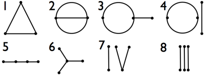
Figure 1: Diagrams corresponding to the cubic cumulants ${\mathcal{W}}$.

We have thus only three possible values of $G$,

$$G_{ab,ab}=G_{1}\,,\ \ G_{ab,ac}=G_{2}\,,\ \ G_{ab,cd}=G_{3}\ ,$$ (74)

and eight possible values of $\mathcal{W}$ as pictorially listed in fig. 1:

$${\mathcal{W}}_{ab,bc,ca}={\mathcal{W}}_{1}\,,\ \ {\mathcal{W}}_{ab,ab,ab}={\mathcal{W}}_{2}\,,\ \ {\mathcal{W}}_{ab,ab,ac}={\mathcal{W}}_{3}\,,\ \ {\mathcal{W}}_{ab,ab,cd}={\mathcal{W}}_{4}\,,\ \$$ (75)

$${\mathcal{W}}_{ab,ac,bd}={\mathcal{W}}_{5}\,,\ \ {\mathcal{W}}_{ab,ac,ad}={\mathcal{W}}_{6}\,,\ \ {\mathcal{W}}_{ac,bc,de}={\mathcal{W}}_{7}\,,\ \ {\mathcal{W}}_{ab,cd,ef}={\mathcal{W}}_{8}\,,\ \$$ (76)

We want to recast the cubic part of the free energy in the following form:

$$\sum_{(ab),(cd),(ef)}{\mathcal{W}}_{ab,cd,ef}\lambda_{ab}\lambda_{cd}\lambda_{ef} = \omega_{1}\sum_{abc}\lambda_{ab}\lambda_{bc}\lambda_{ca}+\omega_{2}\sum_{ab}\lambda_{ab}^{3}+$$ (77)

$$+ \omega_{3}\sum_{abc}\lambda_{ab}^{2}\lambda_{ac}+\omega_{4}\sum_{abcd}\lambda_{ab}^{2}\lambda_{cd}+\omega_{5}\sum_{abcd}\lambda_{ab}\lambda_{ac}\lambda_{bd}+$$

$$+ \omega_{6}\sum_{abcd}\lambda_{ab}\lambda_{ac}\lambda_{ad}+\omega_{7}\sum_{abcde}\lambda_{ac}\lambda_{bc}\lambda_{de}+\omega_{8}\sum_{abcdef}\lambda_{ab}\lambda_{cd}\lambda_{ef}\,.$$

The above identity leads to the following relationships between the $\omega$’s and the ${\mathcal{W}}$’s Temesvári et al. (2002):

$$\omega_{1} = {\mathcal{W}}_{1}-3{\mathcal{W}}_{5}+3{\mathcal{W}}_{7}-{\mathcal{W}}_{8}$$ (78)

$$\omega_{2} = {1\over 2}{\mathcal{W}}_{2}-3{\mathcal{W}}_{3}+{3\over 2}{\mathcal{W}}_{4}+3{\mathcal{W}}_{5}+2{\mathcal{W}}_{6}-6{\mathcal{W}}_{7}+2{\mathcal{W}}_{8}$$ (79)

$$\omega_{3} = 3{\mathcal{W}}_{3}-3{\mathcal{W}}_{4}-6{\mathcal{W}}_{5}-3{\mathcal{W}}_{6}+15{\mathcal{W}}_{7}-6{\mathcal{W}}_{8}$$ (80)

$$\omega_{4} = {3\over 4}({\mathcal{W}}_{4}-2{\mathcal{W}}_{7}+{\mathcal{W}}_{8})$$ (81)

$$\omega_{5} = 3{\mathcal{W}}_{5}-6{\mathcal{W}}_{7}+3{\mathcal{W}}_{8}$$ (82)

$$\omega_{6} = {\mathcal{W}}_{6}-3{\mathcal{W}}_{7}+2{\mathcal{W}}_{8}$$ (83)

$$\omega_{7} = {3\over 2}{\mathcal{W}}_{7}-{3\over 2}{\mathcal{W}}_{8}$$ (84)

$$\omega_{8} = {1\over 8}{\mathcal{W}}_{8}$$ (85)

From the definition (70) we easily see that the coefficients of $F(\lambda)$ can be related to spin averages, in particular $G$ is precisely the dressed propagator:

$$G_{(ab),(cd)}\equiv-{\partial^{2}\over\partial\lambda_{ab}\partial\lambda_{cd}}F(\lambda)=N\langle\delta\tilde{Q}_{ab}\delta\tilde{Q}_{cd}\rangle$$ (86)

In the following and in the previous expression averages are always computed at $\lambda_{ab}=0$. Assuming that we are in a replica symmetric phase we obtain that $G_{(ab),(cd)}$ can take three possible values depending on whether there are two, three or four different replica indexes. The corresponding values are:

$$G_{1} \equiv N\langle\delta\tilde{Q}_{12}^{2}\rangle={1\over N}\sum_{ij}(\overline{\langle s_{i}s_{j}\rangle^{2}}-q^{2})$$ (87)

$$G_{2} \equiv N\langle\delta\tilde{Q}_{12}\delta\tilde{Q}_{13}\rangle={1\over N}\sum_{ij}(\overline{\langle s_{i}s_{j}\rangle\langle{s_{i}}\rangle\langle{s_{j}}\rangle}-q^{2})$$ (88)

$$G_{3} \equiv N\langle\delta\tilde{Q}_{12}\delta\tilde{Q}_{34}\rangle={1\over N}\sum_{ij}(\overline{\langle{s_{i}}\rangle^{2}\langle{s_{j}}\rangle^{2}}-q^{2})$$ (89)

The cubic terms are given by the third derivative:

$${\mathcal{W}}_{(ab),(cd),(ef)}\equiv-{\partial^{3}\over\partial\lambda_{ab}\partial\lambda_{cd}\partial\lambda_{ef}}F(\lambda)=N^{2}\langle\delta\tilde{Q}_{ab}\delta\tilde{Q}_{cd}\delta\tilde{Q}_{ef}\rangle_{c}=N^{2}\langle\delta\tilde{Q}_{ab}\delta\tilde{Q}_{cd}\delta\tilde{Q}_{ef}\rangle$$ (90)

where the suffix $c$ stands for connected functions with respect to the overlaps (not with respect to the spins) and the second equality follows from the fact that the average of $\delta\tilde{Q}_{ab}$ is zero by definition. The cubic cumulants can take eight possible values:

$${\mathcal{W}}_{1} = N^{2}\langle\delta\tilde{Q}_{12}\delta\tilde{Q}_{23}\delta\tilde{Q}_{31}\rangle=$$ (91)

$$= {1\over N}\sum_{ijk}\overline{\langle s_{i}s_{j}\rangle\langle s_{j}s_{k}\rangle\langle s_{k}s_{i}\rangle}-{3q}\sum_{ij}\overline{\langle s_{i}s_{j}\rangle\langle{s_{i}}\rangle\langle{s_{j}}\rangle}+2N^{2}q^{3}$$

$${\mathcal{W}}_{2} = {N^{2}}\langle\delta\tilde{Q}_{12}^{3}\rangle=$$ (92)

$$= {1\over N}\sum_{ijk}\overline{\langle s_{i}s_{j}s_{k}\rangle^{2}}-{3q}\sum_{ij}\overline{\langle s_{i}s_{j}\rangle^{2}}+2N^{2}q^{3}$$

$${\mathcal{W}}_{3} = {N^{2}}\langle\delta\tilde{Q}^{2}_{12}\delta\tilde{Q}_{13}\rangle=$$ (93)

$$= {1\over N}\sum_{ijk}\overline{\langle s_{i}s_{j}s_{k}\rangle\langle s_{i}s_{j}\rangle\langle s_{k}\rangle}-{2q}\sum_{ij}\overline{\langle s_{i}s_{j}\rangle\langle s_{i}\rangle\langle s_{j}\rangle}-{q}\sum_{ij}\overline{\langle s_{i}s_{j}\rangle^{2}}+2N^{2}q^{3}$$

$${\mathcal{W}}_{4} = {N^{2}}\langle\delta\tilde{Q}_{12}^{2}\delta\tilde{Q}_{34}\rangle=$$ (94)

$$= {1\over N}\sum_{ijk}\overline{\langle s_{i}s_{j}\rangle^{2}\langle s_{k}\rangle^{2}}-{2q}\sum_{ij}\overline{\langle s_{i}\rangle^{2}\langle s_{j}\rangle^{2}}-{q}\sum_{ij}\overline{\langle s_{i}s_{j}\rangle^{2}}+2N^{2}q^{3}$$

$${\mathcal{W}}_{5} = {N^{2}}\langle\delta\tilde{Q}_{12}\delta\tilde{Q}_{13}\delta\tilde{Q}_{24}\rangle=$$ (95)

$$= {1\over N}\sum_{ijk}\overline{\langle s_{i}s_{j}\rangle\langle s_{i}s_{k}\rangle\langle s_{k}\rangle\langle s_{j}\rangle}-{2q}\sum_{ij}\overline{\langle s_{i}s_{j}\rangle\langle s_{i}\rangle\langle s_{j}\rangle}-{q}\sum_{ij}\overline{\langle s_{i}\rangle^{2}\langle s_{j}\rangle^{2}}+2N^{2}q^{3}$$

$${\mathcal{W}}_{6} = {N^{2}}\langle\delta\tilde{Q}_{12}\delta\tilde{Q}_{13}\delta\tilde{Q}_{14}\rangle=$$ (96)

$$= {1\over N}\sum_{ijk}\overline{\langle s_{i}s_{j}s_{k}\rangle\langle s_{i}\rangle\langle s_{j}\rangle\langle s_{k}\rangle}-{3q}\sum_{ij}\overline{\langle s_{i}s_{j}\rangle\langle s_{i}\rangle\langle s_{j}\rangle}+2N^{2}q^{3}$$

$${\mathcal{W}}_{7} = {N^{2}}\langle\delta\tilde{Q}_{12}\delta\tilde{Q}_{13}\delta\tilde{Q}_{45}\rangle=$$ (97)

$$= {1\over N}\sum_{ijk}\overline{\langle s_{i}s_{j}\rangle\langle s_{k}\rangle^{2}\langle s_{i}\rangle\langle s_{j}\rangle}-{2q}\sum_{ij}\overline{\langle s_{i}\rangle^{2}\langle s_{j}\rangle^{2}}-{q}\sum_{ij}\overline{\langle s_{i}s_{j}\rangle\langle s_{i}\rangle\langle s_{j}\rangle}+2N^{2}q^{3}$$

$${\mathcal{W}}_{8} = {N^{2}}\langle\delta\tilde{Q}_{12}\delta\tilde{Q}_{34}\delta\tilde{Q}_{56}\rangle=$$ (98)

$$= {1\over N}\sum_{ijk}\overline{\langle s_{i}\rangle^{2}\langle s_{j}\rangle^{2}\langle s_{k}\rangle^{2}}-{3q}\sum_{ij}\overline{\langle s_{i}\rangle^{2}\langle s_{j}\rangle^{2}}+2N^{2}q^{3}$$

Substituting the above expressions in the relationship between the $\omega$’s and the ${\mathcal{W}}$ we obtain:

$$\omega_{1} = {1\over N}\sum_{ijk}\overline{\langle s_{i}s_{j}\rangle_{c}\langle s_{j}s_{k}\rangle_{c}\langle s_{k}s_{i}\rangle_{c}}$$ (99)

$$\omega_{2} = {1\over 2N}\sum_{ijk}\overline{\langle s_{i}s_{j}s_{k}\rangle_{c}^{2}}$$ (100)

$$\omega_{3} = {3\over N}\sum_{ijk}\overline{\langle s_{i}s_{j}s_{k}\rangle_{c}\langle s_{i}s_{j}\rangle_{c}\langle s_{k}\rangle}$$ (101)

$$\omega_{4} = {3\over 4N}\sum_{ijk}\left[\overline{\langle s_{i}s_{j}\rangle_{c}^{2}\langle s_{k}\rangle^{2}}-\overline{\langle s_{i}s_{j}\rangle_{c}^{2}}\ \overline{\langle s_{k}\rangle^{2}}\right]$$ (102)

$$\omega_{5} = {3\over N}\sum_{ijk}\overline{\langle s_{i}s_{j}\rangle_{c}\langle s_{i}s_{k}\rangle_{c}\langle s_{k}\rangle\langle s_{j}\rangle}$$ (103)

$$\omega_{6} = {1\over N}\sum_{ijk}\overline{\langle s_{i}s_{j}s_{k}\rangle_{c}\langle s_{i}\rangle\langle s_{j}\rangle\langle s_{k}\rangle}$$ (104)

$$\omega_{7} = {3\over 2N}\sum_{ijk}\left[\overline{\langle s_{i}s_{j}\rangle_{c}\langle s_{i}\rangle\langle s_{j}\rangle\langle s_{k}\rangle^{2}}-\overline{\langle s_{i}s_{j}\rangle_{c}\langle s_{i}\rangle\langle s_{j}\rangle}\ \overline{\langle s_{k}\rangle^{2}}\right]$$ (105)

$$\omega_{8} = {N^{2}\over 8}\overline{\left(q_{J}-q\right)^{3}}$$ (106)

We note that upon passing from the ${\mathcal{W}}$’s to the $\omega$’s there is increase in symmetry and simplicity, in particular we see that due to various cancellations $\omega_{1}$, $\omega_{2}$, $\omega_{3}$, $\omega_{5}$ and $\omega_{6}$ have a single disorder average, $\omega_{4}$ and $\omega_{7}$ have two disorder average and only $\omega_{8}$ has three disorder averages.

We now turn to the fourth order contribution that involves the $23$ diagrams shown in Fig. (2). These same diagrams have been also studied by Temesvari (see Appendix A in Temesvári (2007), note that we use a different name convention).

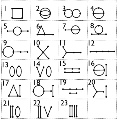
Figure 2: Diagrams corresponding to the quartic cumulants $\mathcal{Y}$.

The expressions of the cumulants ${\mathcal{Y}}_{ab,cd,ef,gh}$ in terms of the physical observables can be obtained by differentiation as we did before for the third order, cf. Eq. (91-98). Again, we are not interested directly in the ${\mathcal{Y}}$ cumulants but, rather, in those linear combinations of theirs corresponding to the unrestricted sums over replicas indexes. In other words, we want to determine the $23$ connected correlation functions $\upsilon_{i}$ that satisfy the following equation:

$${1\over 24}\sum_{(ab),(cd),(ef),(gh)}{\mathcal{Y}}_{ab,cd,ef,gh}\lambda_{ab}\lambda_{cd}\lambda_{ef}\lambda_{gh}={1\over 24}\left[\upsilon_{1}{\rm Tr}\,\lambda^{4}+\upsilon_{2}\sum_{ab}\lambda_{ab}^{4}+\upsilon_{3}\sum_{abc}\lambda_{ab}^{2}\lambda_{ac}^{2}+\upsilon_{4}\sum_{abc}\lambda_{ab}^{2}\lambda_{ac}\lambda_{cb}+\dots\right]$$ (107)

Inasmuch as in the cubic case, we should first associate to the coefficients ${\mathcal{Y}}_{i}$ the appropriate averages of the overlap (corresponding to Eqs. (91-98) for the third order) and then separately determine the connection between the ${\mathcal{Y}}_{i}$’s and the $\upsilon_{i}$. Both computations are reported in Appendix A. The results can, then, be used to derive the analog of expressions (99-106). In spite of the complexity of the intermediate passages it turns out that the result is particularly simple for the four terms explicitly included in Eq. (II), only three of which are those relevant to compute the $\mu$ coefficient of the logarithmic decay. We find:

$$\upsilon_{1} = {3\over N}\sum_{ijkl}\overline{\langle s_{i}s_{j}\rangle_{c}\langle s_{j}s_{k}\rangle_{c}\langle s_{k}s_{l}\rangle_{c}\langle s_{l}s_{i}\rangle_{c}}$$ (108)

$$\upsilon_{2} = {1\over 2N}\sum_{ijkl}\overline{\langle s_{i}s_{j}s_{k}s_{l}\rangle_{c}^{2}}$$ (109)

$$\upsilon_{3} = {3\over N}\sum_{ijkl}\overline{\langle s_{i}s_{j}s_{k}s_{l}\rangle_{c}\langle s_{i}s_{j}\rangle_{c}\langle s_{k}s_{l}\rangle_{c}}$$ (110)

$$\upsilon_{4} = {6\over N}\sum_{ijk}\overline{\langle s_{i}s_{j}s_{k}\rangle_{c}\langle s_{i}s_{j}s_{l}\rangle_{c}\langle s_{l}s_{k}\rangle_{c}}\ .$$ (111)

We are now in position to discuss why we retained only two cubic diagrams and four quartic diagrams in the Gibbs free energy (II). The key point is that the dynamical correlation $\delta Q(1,2)$, for all the three transitions outlined in sec. II, for $n=0,1$, satisfies the relationship

$$\int d1\,Q(1,2)=\delta C(0)+(n-1)\delta C(\infty)=0$$ (112)

because $\delta C(0)=\delta C(\infty)=0$. More generically, one can argue that any object formed from $\delta Q(1,2)$ by means of products and index integrations, that depends only on one index, e.g.

$$A(1)\equiv\int[\delta Q(1,2)]^{5}\ [\delta Q(2,3)]^{6}\ \ \delta Q(2,4)\ \delta Q(4,1)\ d2\ d3\ d4\ ,$$ (113)

vanishes because, upon computing it, one ends up with an expression that only depends on powers of $\delta C(0)$ and $\delta C(\infty)$. Actually, this is the same expression that one would obtain plugging into the above expression a replica symmetric matrix with diagonal elements equal to $\delta C(0)$ and off-diagonal elements equal to $\delta C(\infty)$.

The same is naturally true for objects that depend on no index at all. Therefore, we can neglect all disconnected diagrams in the Gibbs free energy as they lead to terms containing factors that do not depend on either $1$ or $2$ in the equation (III) obtained by differentiation with respect to $\delta Q(1,2)$.

For the same reason, we can also neglect diagrams with dangling hands in the Gibbs free energy. Indeed, they contribute two types of terms to the equation: either a term with a dangling hand (that vanishes because of Eq. (112)) or terms that depends only on index $1$ or $2$ separately and, thus, vanish. More generically, any diagram that can be disconnected removing one vertex yields a vanishing contribution.

Diagrams with dangling hands are the simplest diagrams satisfying this property but not the only ones. Indeed, consistently, we could have also ignored the term proportional to $y_{3}$ in expression (II) from the beginning, since removing the central vertex in the third diagram in Fig. 2 we have two disconnected graphs.

V Inversion of the Legendre Transform: relations between cumulants and vertex coefficients.

In this section we express the coefficients of the Gibbs free energy in terms of those of the free energy obtained in the previous section. The Gibbs Free energy is defined as the Legendre transform of the Free energy $F(\lambda)$:

$$G(\delta Q)\equiv F(\lambda)+\sum_{(ab)}\lambda_{ab}\delta Q_{ab}$$ (114)

where $\lambda$ is a function of $\delta Q_{ab}$ according to the following implicit equation:

$$\delta Q_{ab}=-{\partial F\over\partial\lambda_{ab}}.$$ (115)

On the other hand, the free energy $F$ is the Legendre transform of the Gibbs free energy $G$ with:

$$\lambda_{ab}={\partial G\over\partial\delta Q_{ab}}\ .$$ (116)

We consider the free energy expansion Eq. (73), taking into account only those terms eventually relevant to describe the critical slowing down:

$$F(\lambda) = -{1\over 2}\sum_{(ab),(cd)}\lambda_{ab}G_{ab,cd}\lambda_{cd}$$

$$-\frac{\omega_{1}}{6}\omega_{1}{\rm Tr}\,\lambda^{3}-\frac{\omega_{2}}{6}\sum_{ab}\lambda_{ab}^{3}$$

$$-\frac{\upsilon_{1}}{24}{\rm Tr}\,\lambda^{4}-\frac{\upsilon_{2}}{24}\sum_{ab}\lambda^{4}_{ab}$$

$$-\frac{\upsilon_{4}}{24}\sum_{abc}\lambda_{ab}^{2}\lambda_{ac}\lambda_{ef}$$

leading to

$$\delta Q_{ab} = -\frac{\partial F}{\partial\lambda_{ab}}=G_{(ab)(cd)}\lambda_{cd}$$

$$+\omega_{1}(\lambda^{2})_{ab}+\omega_{2}\lambda_{ab}^{2}$$

$$+\frac{\upsilon_{1}}{3}(\lambda^{3})_{ab}+\frac{\upsilon_{2}}{3}\lambda_{ab}^{3}$$

$$+\frac{\upsilon_{4}}{6}\lambda_{ab}(\lambda^{2})_{ab}+\frac{\upsilon_{4}}{12}\sum_{c}\left(\lambda_{ac}^{2}\lambda_{cb}+\lambda^{2}_{bc}\lambda_{ca}\right)$$

where

$$G_{(ab)(cd)}=\left\{\begin{array}[]{ll}G_{1}&(ab)=(cd)\\ G_{2}&(b=d)\vee(a=c)\\ G_{3}&a\neq c\wedge b\neq d\end{array}\right.$$ (119)

The inverse $M=G^{-1}$ matrix displays the generic form

$$M_{(ab)(cd)} = r\left(\delta_{ac}\delta_{bd}+\delta_{ad}\delta_{bc}\right)$$

$$+(M_{2}-M_{3})\left(\delta_{ac}+\delta_{ad}+\delta_{bc}+\delta_{bd}\right)$$

$$+M_{3}$$

with

$$r\equiv M_{1}-2M_{2}+M_{3}=\frac{1}{G_{1}-2G_{2}+G_{3}}$$ (121)

Using the above properties and neglecting terms without both indexes $a$ and $b$ (irrelevant in the present context) we can invert Eq. (V) yielding, to the fourth order

$$\lambda_{ab} = r\delta Q_{ab}-\omega_{1}r^{3}\left(\delta Q^{2}\right)_{ab}-\omega_{2}r^{3}\delta Q_{ab}^{3}$$

$$+\left(2r^{5}\omega_{1}^{2}-r^{4}\frac{\upsilon_{1}}{3}\right)\left(\delta Q^{3}\right)_{ab}$$

$$+\left(2r^{5}\omega_{2}^{2}-r^{4}\frac{\upsilon_{2}}{3}\right)\delta Q_{ab}^{3}$$

$$+\left(r^{5}\omega_{1}\omega_{2}-r^{4}\frac{\upsilon_{4}}{12}\right)\sum_{c}\left(\delta Q_{ac}^{2}\delta Q_{cb}+\delta Q_{ac}\delta Q_{cb}^{2}\right)$$

$$+\left(2r^{5}\omega_{1}\omega_{2}-r^{4}\frac{\upsilon_{4}}{6}\right)\delta Q_{ab}\left(\delta Q^{2}\right)_{ab}$$

Comparing the above expression with Eqs. (II), (III) we find the relationships between the cumulants $\omega$, $\upsilon$ and the vertex coefficients $w$,$y$

$$y_{1} = -6r^{5}\omega_{1}^{2}+r^{4}\upsilon_{1}$$ (123)

$$y_{2} = -6r^{5}\omega_{2}^{2}+r^{4}\upsilon_{2}$$ (124)

$$y_{4} = -12r^{5}\omega_{1}\omega_{2}+r^{4}\upsilon_{4}$$ (125)

$$w_{1} = r^{3}\omega_{1}$$ (126)

$$w_{2} = r^{3}\omega_{2}$$ (127)

At the tricritical point, Tthe expression for the logarithmic decay parameter $\mu$, cf. Eq. (17) can, thus, be expressed in terms of cumulants as

$$\mu=-\frac{y_{1}+y_{2}-y_{4}}{3w_{1}}=-r\frac{\upsilon_{1}+\upsilon_{2}-\upsilon_{4}}{3\omega_{1}}\,,\ \ \ (\lambda=1)$$ (128)

where we explicitly used the fact that the exponent parameter is $\lambda=1=\omega_{2}/\omega_{1}$. From Eqs. (123)-(127) we notice that though each vertex coefficient singularly diverges as $r^{-5}$, their combination $y_{1}+y_{2}-y_{4}$, for $w_{1}=w_{2}$, diverges as $r^{-4}$, thus yielding a finite $\mu$ when power-law critical slowing down (described by means of the third order expansion when $\lambda\neq 1$) is no longer defined. To clearly see this we can express the quartic susceptibilities in term of the coupling constants:

$$\upsilon_{1}+\upsilon_{2}-\upsilon_{4}=6\frac{(w_{1}-w_{2})^{2}}{r^{5}}+\frac{y_{1}+y_{2}-y_{4}}{r^{4}}$$ (129)

This shows that whenever $w_{1}\neq w_{2}$ the critical behaviour of the quartic susceptibility is $O(r^{-5})$ and it is controlled by the cubic coupling constants. Instead, when $w_{1}=w_{2}$ the quartic susceptibility is less divergent $O(r^{-4})$ and it is controlled by the quartic coupling constants.

VI Conclusions

In this paper we have demonstrated that the structure of the replicated Gibbs free energy near a critical point characterized by $w_{1}=w_{2}$ implies a logarithmic decay of dynamical correlations. This allows to characterize the asymptotic critical dynamics in a variety of systems where the equilibrium statics can be studied by means of the replica method but the microscopic dynamical equations are difficult to be solved, including Ising spin-glass models, Potts spin-glass models and hard-spheres model in the limit of infinite dimension.

The connection between static and dynamics is also quantitative, in the sense that the parameter controlling the logarithmic decay can be read from the static Gibbs free energy and, thus, it can be expressed in terms of connected correlation functions of the overlap fluctuations that can be measured statically from equilibrium configurations. This is significant from the point of view of numerical simulations of glassy systems, as often one can use clever algorithms to obtain equilibrium configurations much faster than the standard dynamical microscopic evolution Marinari and Parisi (1992); Hukushima and Nemoto (1996); Ninarello et al. (2017).

The emergence of logarithmic slowing down, being a consequence solely of the Gibbs free energy structure, has a great deal of universality. Indeed many models, that can be utterly different from each other at the microscopic level, can in principle be described by the same Landau theory. Note that we have written the expression of $\mu$ in terms of observables for spin systems but it can be easily rewritten for particles systems as we explained in section II. Thus the relationship between $\mu$ and experimental observables is completely general: it would be important to work out in full the connection between these cumulants and higher-order non-linear susceptibilities that can be measured in experiments Albert et al. (2019).

It is also interesting to mention two instances in which there is instead no connection between logarithmic slowing down and connected correlation functions of the overlap fluctuations. This is provided by Fredrikson-Andersen Kinetically constrained model on the Bethe lattice with either random pinning Ikeda et al. (2017) or with non-homogeneous facilitation Sellitto et al. (2010); Arenzon and Sellitto (2012): the analytical solution of these models Perrupato and Rizzo (2022) has indeed allowed to demonstrate and quantify the logarithmic slowing down as given by eq. (16) but a thermodynamic analysis of the model has revealed that there is no connection between the observed MCT-like dynamics and connected correlation functions of the overlap that are not divergent at the critical point Perrupato and Rizzo (2023), i.e. eq. (18) does not hold.

As a final technical remark we note that upon passing from restricted to unrestricted replica summations the corresponding coefficients considerably simplify. This can be seen comparing the coefficients $\mathcal{W}_{i}$ in the free energy expansion (73) with the $\omega_{i}$ in Eq. (77) and comparing the $\mathcal{Y}_{i}$ with the $\upsilon_{i}$ in Eq. (107). It turns out that one can find a simple set of diagrammatic rules to directly compute the unrestricted coefficients, i.e., the $\omega_{i}$, the $\upsilon_{i}$ and those at higher orders, without the lengthy intermediate passages .

Appendix A Fourth order cumulants

The fourth order coefficients of the Free energy read:

$${\mathcal{Y}}_{1} = N^{3}\langle\delta Q_{ab}\delta Q_{bc}\delta Q_{cd}\delta Q_{da}\rangle_{c}$$

$$= \frac{1}{N}\sum_{ijkl}{\overline{\langle s_{i}s_{j}\rangle\langle s_{j}s_{k}\rangle\langle s_{k}s_{l}\rangle\langle s_{l}s_{i}\rangle}}-4q\sum_{ijk}{\overline{\langle s_{i}\rangle\langle s_{i}s_{j}\rangle\langle s_{j}s_{k}\rangle\langle s_{k}\rangle}}$$

$$+2Nq^{2}\sum_{ij}{\overline{\langle s_{i}\rangle^{2}\langle s_{j}\rangle^{2}}}+4Nq^{2}\sum_{ij}{\overline{\langle s_{i}\rangle\langle s_{i}s_{j}\rangle\langle s_{j}\rangle}}-3q^{4}N^{3}-2NG_{2}^{2}-NG_{3}^{2}$$

$${\mathcal{Y}}_{2} = N^{3}\langle\delta Q_{12}^{4}\rangle_{c}$$

$$= \frac{1}{N}\sum_{ijkl}{\overline{\langle s_{i}s_{j}s_{k}s_{l}\rangle^{2}}}-4q\sum_{ijk}{\overline{\langle s_{i}s_{j}s_{k}\rangle^{2}}}+6Nq^{2}\sum_{ij}{\overline{\langle s_{i}s_{j}\rangle^{2}}}-3q^{4}N^{3}-3NG_{1}^{2}$$

$${\mathcal{Y}}_{3} = N^{3}\langle\delta Q_{ab}^{2}\delta Q_{bc}^{2}\rangle_{c}$$

$$= \frac{1}{N}\sum_{ijkl}{\overline{\langle s_{i}s_{j}\rangle\langle s_{i}s_{j}s_{k}s_{l}\rangle\langle s_{k}s_{l}\rangle}}-4q\sum_{ijk}{\overline{\langle s_{i}s_{j}\rangle\langle s_{i}s_{j}s_{k}\rangle\langle s_{k}\rangle}}$$

$$+4Nq^{2}\sum_{ij}{\overline{\langle s_{i}\rangle\langle s_{i}s_{j}\rangle\langle s_{j}\rangle}}+2Nq^{2}\sum_{ij}{\overline{\langle s_{i}s_{j}\rangle^{2}}}-3q^{4}N^{3}-NG_{1}^{2}-2NG_{2}^{2}$$

$${\mathcal{Y}}_{4} = N^{3}\langle\delta Q_{ab}\delta Q_{bc}\delta Q_{ac}^{2}\rangle_{c}$$

$$= \frac{1}{N}\sum_{ijkl}{\overline{\langle s_{i}s_{j}s_{k}\rangle\langle s_{i}s_{j}s_{l}\rangle\langle s_{k}s_{l}\rangle}}-2q\sum_{ijk}{\overline{\langle s_{i}s_{j}\rangle\langle s_{i}s_{j}s_{k}\rangle\langle s_{k}\rangle}}-2q\sum_{ijk}{\overline{\langle s_{i}s_{j}\rangle\langle s_{j}s_{k}\rangle\langle s_{k}s_{i}\rangle}}$$

$$+5Nq^{2}\sum_{ij}{\overline{\langle s_{i}\rangle\langle s_{i}s_{j}\rangle\langle s_{j}\rangle}}+Nq^{2}\sum_{ij}{\overline{\langle s_{i}s_{j}\rangle^{2}}}-3q^{4}N^{3}-NG_{1}G_{2}-2NG_{2}^{2}$$

$${\mathcal{Y}}_{5} = N^{3}\langle\delta Q_{ab}\delta Q_{bc}^{2}\delta Q_{cd}\rangle_{c}$$

$$= \frac{1}{N}\sum_{ijkl}{\overline{\langle s_{i}\rangle\langle s_{i}s_{j}s_{k}\rangle\langle s_{j}s_{k}s_{l}\rangle\langle s_{l}\rangle}}-2q\sum_{ijk}{\overline{\langle s_{i}s_{j}\rangle\langle s_{i}s_{j}s_{k}\rangle\langle s_{k}\rangle}}-2q\sum_{ijk}{\overline{\langle s_{i}\rangle\langle s_{i}s_{j}\rangle\langle s_{j}s_{k}\rangle\langle s_{k}\rangle}}$$

$$+Nq^{2}\sum_{ij}{\overline{\langle s_{i}\rangle^{2}\langle s_{j}\rangle^{2}}}+4Nq^{2}\sum_{ij}{\overline{\langle s_{i}\rangle\langle s_{i}s_{j}\rangle\langle s_{j}\rangle}}+Nq^{2}\sum_{ij}{\overline{\langle s_{i}s_{j}\rangle^{2}}}-3q^{4}N^{3}-2NG_{2}^{2}-NG_{1}G_{3}$$

$${\mathcal{Y}}_{6} = N^{3}\langle\delta Q_{ab}\delta Q_{bc}\delta Q_{ca}\delta Q_{cd}\rangle_{c}$$

$$= \frac{1}{N}\sum_{ijkl}{\overline{\langle s_{i}s_{j}\rangle\langle s_{i}s_{k}s_{l}\rangle\langle s_{k}s_{i}\rangle\langle s_{l}\rangle}}-q\sum_{ijk}{\overline{\langle s_{i}s_{j}s_{k}\rangle\langle s_{i}\rangle\langle s_{j}\rangle\langle s_{k}\rangle}}$$

$$-2q\sum_{ijk}{\overline{\langle s_{i}\rangle\langle s_{i}s_{j}\rangle\langle s_{j}s_{k}\rangle\langle s_{k}\rangle}}-q\sum_{ijk}{\overline{\langle s_{i}s_{j}\rangle\langle s_{j}s_{k}\rangle\langle s_{k}s_{i}\rangle}}$$

$$+Nq^{2}\sum_{ij}{\overline{\langle s_{i}\rangle^{2}\langle s_{j}\rangle^{2}}}+5Nq^{2}\sum_{ij}{\overline{\langle s_{i}\rangle\langle s_{i}s_{j}\rangle\langle s_{j}\rangle}}-3q^{4}N^{3}-2NG_{2}^{2}-NG_{2}G_{3}$$

$${\mathcal{Y}}_{7} = N^{3}\langle\delta Q_{ab}\delta Q_{bc}^{3}\rangle_{c}$$

$$= \frac{1}{N}\sum_{ijkl}{\overline{\langle s_{i}s_{j}s_{k}s_{l}\rangle\langle s_{i}\rangle\langle s_{j}s_{k}s_{l}\rangle}}-q\sum_{ijk}{\overline{\langle s_{i}s_{j}s_{k}\rangle^{2}}}-3q\sum_{ijk}{\overline{\langle s_{i}s_{j}\rangle\langle s_{i}s_{j}s_{k}\rangle\langle s_{k}\rangle}}$$

$$+3Nq^{2}\sum_{ij}{\overline{\langle s_{i}\rangle\langle s_{i}s_{j}\rangle\langle s_{j}\rangle}}+3Nq^{2}\sum_{ij}{\overline{\langle s_{i}s_{j}\rangle^{2}}}-3q^{4}N^{3}-3NG_{1}G_{2}$$

$${\mathcal{Y}}_{8} = N^{3}\langle\delta Q_{ab}\delta Q_{bc}^{2}\delta Q_{bd}\rangle_{c}$$

$$= \frac{1}{N}\sum_{ijkl}{\overline{\langle s_{i}s_{j}s_{k}s_{l}\rangle\langle s_{i}\rangle\langle s_{j}s_{k}\rangle\langle s_{l}\rangle}}-2q\sum_{ijk}{\overline{\langle s_{i}s_{j}s_{k}\rangle\langle s_{i}\rangle\langle s_{j}\rangle\langle s_{k}\rangle}}-2q\sum_{ijk}{\overline{\langle s_{i}s_{j}\rangle\langle s_{i}s_{j}s_{k}\rangle\langle s_{k}\rangle}}$$

$$+5Nq^{2}\sum_{ij}{\overline{\langle s_{i}\rangle\langle s_{i}s_{j}\rangle\langle s_{j}\rangle}}+Nq^{2}\sum_{ij}{\overline{\langle s_{i}s_{j}\rangle^{2}}}-3q^{4}N^{3}-2NG_{2}^{2}-NG_{1}G_{2}$$

$${\mathcal{Y}}_{9} = N^{3}\langle\delta Q_{ab}^{2}\delta Q_{bc}\delta Q_{cd}\rangle_{c}$$

$$= \frac{1}{N}\sum_{ijkl}{\overline{\langle s_{i}s_{j}\rangle\langle s_{i}s_{j}s_{k}\rangle\langle s_{k}s_{l}\rangle\langle s_{l}\rangle}}-2q\sum_{ijk}{\overline{\langle s_{i}\rangle\langle s_{i}s_{j}\rangle\langle s_{j}s_{k}\rangle\langle s_{k}\rangle}}$$

$$-q\sum_{ijk}{\overline{\langle s_{i}s_{j}\rangle^{2}\langle s_{k}\rangle^{2}}}-q\sum_{ijk}{\overline{\langle s_{i}s_{j}\rangle\langle s_{i}s_{j}s_{k}\rangle\langle s_{k}\rangle}}$$

$$+2Nq^{2}\sum_{ij}{\overline{\langle s_{i}\rangle^{2}\langle s_{j}\rangle^{2}}}+3Nq^{2}\sum_{ij}{\overline{\langle s_{i}\rangle\langle s_{i}s_{j}\rangle\langle s_{j}\rangle}}+Nq^{2}\sum_{ij}{\overline{\langle s_{i}s_{j}\rangle^{2}}}-3q^{4}N^{3}-NG_{1}G_{2}-2NG_{2}G_{3}$$

$${\mathcal{Y}}_{10} = N^{3}\langle\delta Q_{ab}\delta Q_{ac}\delta Q_{ad}\delta Q_{ae}\rangle_{c}$$

$$= \frac{1}{N}\sum_{ijkl}{\overline{\langle s_{i}s_{j}s_{k}s_{l}\rangle\langle s_{i}\rangle\langle s_{j}\rangle\langle s_{k}\rangle\langle s_{l}\rangle}}-4q\sum_{ijk}{\overline{\langle s_{i}s_{j}s_{k}\rangle\langle s_{i}\rangle\langle s_{j}\rangle\langle s_{k}\rangle}}$$

$$+6Nq^{2}\sum_{ij}{\overline{\langle s_{i}\rangle\langle s_{i}s_{j}\rangle\langle s_{j}\rangle}}-3q^{4}N^{3}-3NG_{2}^{2}$$

$${\mathcal{Y}}_{11} = N^{3}\langle\delta Q_{ab}\delta Q_{bc}\delta Q_{bd}\delta Q_{de}\rangle_{c}$$

$$= \frac{1}{N}\sum_{ijkl}{\overline{\langle s_{i}\rangle\langle s_{i}s_{j}s_{k}\rangle\langle s_{i}\rangle\langle s_{k}s_{l}\rangle\langle s_{l}\rangle}}-2q\sum_{ijk}{\overline{\langle s_{i}\rangle\langle s_{i}s_{j}\rangle\langle s_{j}s_{k}\rangle\langle s_{k}\rangle}}$$

$$-q\sum_{ijk}{\overline{\langle s_{i}\rangle^{2}\langle s_{j}\rangle\langle s_{j}s_{k}\rangle\langle s_{k}\rangle}}-q\sum_{ijk}{\overline{\langle s_{i}s_{j}s_{k}\rangle\langle s_{i}\rangle\langle s_{j}\rangle\langle s_{k}\rangle}}$$

$$+2Nq^{2}\sum_{ij}{\overline{\langle s_{i}\rangle^{2}\langle s_{j}\rangle^{2}}}+4Nq^{2}\sum_{ij}{\overline{\langle s_{i}\rangle\langle s_{i}s_{j}\rangle\langle s_{j}\rangle}}-3q^{4}N^{3}-NG_{2}^{2}-2NG_{2}G_{3}$$

$${\mathcal{Y}}_{12} = N^{3}\langle\delta Q_{ab}\delta Q_{bc}\delta Q_{cd}\delta Q_{de}\rangle_{c}$$

$$= \frac{1}{N}\sum_{ijkl}{\overline{\langle s_{i}\rangle\langle s_{i}s_{j}\rangle\langle s_{j}s_{k}\rangle\langle s_{k}s_{l}\rangle\langle s_{l}\rangle}}-2q\sum_{ijk}{\overline{\langle s_{i}\rangle\langle s_{i}s_{j}\rangle\langle s_{j}s_{k}\rangle\langle s_{k}\rangle}}$$

$$-2q\sum_{ijk}{\overline{\langle s_{i}\rangle^{2}\langle s_{j}\rangle\langle s_{j}s_{k}\rangle\langle s_{k}\rangle}}+3Nq^{2}\sum_{ij}{\overline{\langle s_{i}\rangle^{2}\langle s_{j}\rangle^{2}}}$$

$$+3Nq^{2}\sum_{ij}{\overline{\langle s_{i}\rangle\langle s_{i}s_{j}\rangle\langle s_{j}\rangle}}-3q^{4}N^{3}-NG_{2}^{2}-NG_{3}^{2}-NG_{2}G_{3}$$

$${\mathcal{Y}}_{13} = N^{3}\langle\delta Q_{ab}^{2}\delta Q_{cd}^{2}\rangle_{c}$$

$$= \frac{1}{N}\sum_{ijkl}{\overline{\langle s_{i}s_{j}\rangle^{2}\langle s_{k}s_{l}\rangle^{2}}}-4q\sum_{ijk}{\overline{\langle s_{i}s_{j}\rangle^{2}\langle s_{k}\rangle^{2}}}$$

$$+4Nq^{2}\sum_{ij}{\overline{\langle s_{i}\rangle^{2}\langle s_{j}\rangle^{2}}}+2Nq^{2}\sum_{ij}{\overline{\langle s_{i}s_{j}\rangle^{2}}}-3q^{4}N^{3}-NG_{1}^{2}-2NG_{3}^{2}$$

$${\mathcal{Y}}_{14} = N^{3}\langle\delta Q_{ab}^{2}\delta Q_{cd}\delta Q_{de}\rangle_{c}$$

$$= \frac{1}{N}\sum_{ijkl}{\overline{\langle s_{i}s_{j}\rangle^{2}\langle s_{k}\rangle\langle s_{k}s_{l}\rangle\langle s_{l}\rangle}}-2q\sum_{ijk}{\overline{\langle s_{i}\rangle^{2}\langle s_{j}\rangle\langle s_{j}s_{k}\rangle\langle s_{k}\rangle}}-2q\sum_{ijk}{\overline{\langle s_{i}s_{j}\rangle^{2}\langle s_{k}\rangle^{2}}}$$

$$+4Nq^{2}\sum_{ij}{\overline{\langle s_{i}\rangle^{2}\langle s_{j}\rangle^{2}}}+Nq^{2}\sum_{ij}{\overline{\langle s_{i}\rangle\langle s_{i}s_{j}\rangle\langle s_{j}\rangle}}+Nq^{2}\sum_{ij}{\overline{\langle s_{i}s_{j}\rangle^{2}}}-3q^{4}N^{3}-NG_{1}G_{2}-2NG_{3}^{2}$$

$${\mathcal{Y}}_{15} = N^{3}\langle\delta Q_{ab}\delta Q_{bc}\delta Q_{de}\delta Q_{ef}\rangle_{c}$$

$$= \frac{1}{N}\sum_{ijkl}{\overline{\langle s_{i}\rangle\langle s_{i}s_{j}\rangle\langle s_{j}\rangle\langle s_{k}\rangle\langle s_{k}s_{l}\rangle\langle s_{l}\rangle}}-4q\sum_{ijk}{\overline{\langle s_{i}\rangle^{2}\langle s_{j}\rangle\langle s_{j}s_{k}\rangle\langle s_{k}\rangle}}$$

$$+4Nq^{2}\sum_{ij}{\overline{\langle s_{i}\rangle^{2}\langle s_{j}\rangle^{2}}}+2Nq^{2}\sum_{ij}{\overline{\langle s_{i}\rangle\langle s_{i}s_{j}\rangle\langle s_{j}\rangle}}-3q^{4}N^{3}-NG_{2}^{2}-2NG_{3}^{2}$$

$${\mathcal{Y}}_{16} = N^{3}\langle\delta Q_{ab}^{3}\delta Q_{cd}\rangle_{c}$$

$$= \frac{1}{N}\sum_{ijkl}{\overline{\langle s_{i}s_{j}s_{k}\rangle^{2}\langle s_{l}\rangle^{2}}}-q\sum_{ijk}{\overline{\langle s_{i}s_{j}s_{k}\rangle^{2}}}-3q\sum_{ijk}{\overline{\langle s_{i}s_{j}\rangle^{2}\langle s_{k}\rangle^{2}}}$$

$$+3Nq^{2}\sum_{ij}{\overline{\langle s_{i}\rangle^{2}\langle s_{j}\rangle^{2}}}+3Nq^{2}\sum_{ij}{\overline{\langle s_{i}s_{j}\rangle^{2}}}-3q^{4}N^{3}-3NG_{1}G_{3}$$

$${\mathcal{Y}}_{17} = N^{3}\langle\delta Q_{ab}\delta Q_{bc}\delta Q_{ca}\delta Q_{de}\rangle_{c}$$

$$= \frac{1}{N}\sum_{ijkl}{\overline{\langle s_{i}s_{j}\rangle\langle s_{j}s_{k}\rangle\langle s_{k}s_{i}\rangle\langle s_{l}\rangle^{2}}}-3q\sum_{ijk}{\overline{\langle s_{i}\rangle^{2}\langle s_{j}\rangle\langle s_{j}s_{k}\rangle\langle s_{k}\rangle}}-q\sum_{ijk}{\overline{\langle s_{i}s_{j}\rangle\langle s_{j}s_{k}\rangle\langle s_{k}s_{i}\rangle}}$$

$$+3Nq^{2}\sum_{ij}{\overline{\langle s_{i}\rangle^{2}\langle s_{j}\rangle^{2}}}+3Nq^{2}\sum_{ij}{\overline{\langle s_{i}\rangle\langle s_{i}s_{j}\rangle\langle s_{j}\rangle}}-3q^{4}N^{3}-3NG_{2}G_{3}$$

$${\mathcal{Y}}_{18} = N^{3}\langle\delta Q_{ab}^{2}\delta Q_{bc}\delta Q_{de}\rangle_{c}$$

$$= \frac{1}{N}\sum_{ijkl}{\overline{\langle s_{i}s_{j}\rangle\langle s_{i}s_{j}s_{k}\rangle\langle s_{k}\rangle\langle s_{l}\rangle^{2}}}-2q\sum_{ijk}{\overline{\langle s_{i}\rangle^{2}\langle s_{j}\rangle\langle s_{j}s_{k}\rangle\langle s_{k}\rangle}}$$

$$-q\sum_{ijk}{\overline{\langle s_{i}s_{j}\rangle^{2}\langle s_{k}\rangle^{2}}}-q\sum_{ijk}{\overline{\langle s_{i}s_{j}\rangle\langle s_{i}s_{j}s_{k}\rangle\langle s_{k}\rangle}}$$

$$+3Nq^{2}\sum_{ij}{\overline{\langle s_{i}\rangle^{2}\langle s_{j}\rangle^{2}}}+2Nq^{2}\sum_{ij}{\overline{\langle s_{i}\rangle\langle s_{i}s_{j}\rangle\langle s_{j}\rangle}}+Nq^{2}\sum_{ij}{\overline{\langle s_{i}s_{j}\rangle^{2}}}-3q^{4}N^{3}-NG_{1}G_{3}-2NG_{2}G_{3}$$

$${\mathcal{Y}}_{19} = N^{3}\langle\delta Q_{ab}\delta Q_{bc}\delta Q_{cd}\delta Q_{ef}\rangle_{c}$$

$$= \frac{1}{N}\sum_{ijkl}{\overline{\langle s_{i}\rangle\langle s_{i}s_{j}\rangle\langle s_{j}s_{k}\rangle\langle s_{k}\rangle\langle s_{l}\rangle^{2}}}-2q\sum_{ijk}{\overline{\langle s_{i}\rangle^{2}\langle s_{j}\rangle\langle s_{j}s_{k}\rangle\langle s_{k}\rangle}}$$

$$-q\sum_{ijk}{\overline{\langle s_{i}\rangle^{2}\langle s_{j}\rangle^{2}\langle s_{k}\rangle^{2}}}-q\sum_{ijk}{\overline{\langle s_{i}\rangle\langle s_{i}s_{j}\rangle\langle s_{j}s_{k}\rangle\langle s_{k}\rangle}}$$

$$+4Nq^{2}\sum_{ij}{\overline{\langle s_{i}\rangle^{2}\langle s_{j}\rangle^{2}}}+2Nq^{2}\sum_{ij}{\overline{\langle s_{i}\rangle\langle s_{i}s_{j}\rangle\langle s_{j}\rangle}}-3q^{4}N^{3}-2NG_{2}G_{3}-NG3^{2}$$

$${\mathcal{Y}}_{20} = N^{3}\langle\delta Q_{ab}\delta Q_{ac}\delta Q_{ad}\delta Q_{ef}\rangle_{c}$$

$$= \frac{1}{N}\sum_{ijkl}{\overline{\langle s_{i}s_{j}s_{k}\rangle\langle s_{i}\rangle\langle s_{j}\rangle\langle s_{k}\rangle\langle s_{l}\rangle^{2}}}-3q\sum_{ijk}{\overline{\langle s_{i}\rangle^{2}\langle s_{j}\rangle\langle s_{j}s_{k}\rangle\langle s_{k}\rangle}}-q\sum_{ijk}{\overline{\langle s_{i}s_{j}s_{k}\rangle\langle s_{i}\rangle\langle s_{j}\rangle\langle s_{k}\rangle}}$$

$$+3Nq^{2}\sum_{ij}{\overline{\langle s_{i}\rangle\langle s_{i}s_{j}\rangle\langle s_{j}\rangle}}+3Nq^{2}\sum_{ij}{\overline{\langle s_{i}\rangle^{2}\langle s_{j}\rangle^{2}}}-3q^{4}N^{3}-3NG_{2}G_{3}$$

$${\mathcal{Y}}_{21} = N^{3}\langle\delta Q_{ab}\delta Q_{cd}\delta Q_{ef}^{2}\rangle_{c}$$

$$= \frac{1}{N}\sum_{ijkl}{\overline{\langle s_{i}\rangle^{2}\langle s_{j}\rangle^{2}\langle s_{k}s_{l}\rangle^{2}}}-2q\sum_{ijk}{\overline{\langle s_{i}\rangle^{2}\langle s_{j}s_{k}\rangle^{2}}}-2q\sum_{ijk}{\overline{\langle s_{i}\rangle^{2}\langle s_{j}\rangle^{2}\langle s_{k}\rangle^{2}}}$$

$$+5Nq^{2}\sum_{ij}{\overline{\langle s_{i}\rangle^{2}\langle s_{j}\rangle^{2}}}+Nq^{2}\sum_{ij}{\overline{\langle s_{i}s_{j}\rangle^{2}}}-3q^{4}N^{3}-NG_{1}G_{3}-2NG_{3}^{2}$$

$${\mathcal{Y}}_{22} = N^{3}\langle\delta Q_{ab}\delta Q_{cd}\delta Q_{ef}\delta Q_{fg}\rangle_{c}$$

$$= \frac{1}{N}\sum_{ijkl}{\overline{\langle s_{i}\rangle^{2}\langle s_{j}\rangle^{2}\langle s_{k}\rangle\langle s_{k}s_{l}\rangle\langle s_{l}\rangle}}-2q\sum_{ijk}{\overline{\langle s_{i}\rangle^{2}\langle s_{j}\rangle\langle s_{j}s_{k}\rangle\langle s_{k}\rangle}}-2q\sum_{ijk}{\overline{\langle s_{i}\rangle^{2}\langle s_{j}\rangle^{2}\langle s_{k}\rangle^{2}}}$$

$$+Nq^{2}\sum_{ij}{\overline{\langle s_{i}\rangle\langle s_{i}s_{j}\rangle\langle s_{j}\rangle}}+5Nq^{2}\sum_{ij}{\overline{\langle s_{i}\rangle^{2}\langle s_{j}\rangle^{2}}}-3q^{4}N^{3}-NG_{2}G_{3}-2NG_{3}^{2}$$

$${\mathcal{Y}}_{23} = N^{3}\langle\delta Q_{ab}\delta Q_{cd}\delta Q_{ef}\delta Q_{gh}\rangle$$

$$= \frac{1}{N}\sum_{ijkl}{\overline{\langle s_{i}\rangle^{2}\langle s_{j}\rangle^{2}\langle s_{k}\rangle^{2}\langle s_{l}\rangle^{2}}}-4q\sum_{ijk}{\overline{\langle s_{i}\rangle^{2}\langle s_{j}\rangle^{2}\langle s_{k}\rangle^{2}}}+6Nq^{2}\sum_{ij}{\overline{\langle s_{i}\rangle^{2}\langle s_{j}\rangle^{2}}}-3q^{4}N^{3}-3NG_{3}^{2}$$

Counting the multiplicity of each apart term, the above coefficients in Eq. (107) recombine according to the following formulas (they are equal to those of Appendix B in Temesvári (2007) taking into account for the different naming convention).

$$\upsilon_{1} = 3({\mathcal{Y}}_{1}-4{\mathcal{Y}}_{12}+2{\mathcal{Y}}_{15}+4{\mathcal{Y}}_{19}-4{\mathcal{Y}}_{22}+{\mathcal{Y}}_{23})$$ (154)

$$\upsilon_{2} = \frac{1}{2}(6{\mathcal{Y}}_{1}-12{\mathcal{Y}}_{10}-48{\mathcal{Y}}_{11}-48{\mathcal{Y}}_{12}+3{\mathcal{Y}}_{13}-24{\mathcal{Y}}_{14}+60{\mathcal{Y}}_{15}+4{\mathcal{Y}}_{16}-48{\mathcal{Y}}_{18}$$

$$+96{\mathcal{Y}}_{19}+{\mathcal{Y}}_{2}+48{\mathcal{Y}}_{20}+24{\mathcal{Y}}_{21}-144{\mathcal{Y}}_{22}+36{\mathcal{Y}}_{23}-6{\mathcal{Y}}_{3}+12{\mathcal{Y}}_{5}-8{\mathcal{Y}}_{7}+24{\mathcal{Y}}_{8}+24{\mathcal{Y}}_{9})$$

$$\upsilon_{3} = 3(-2{\mathcal{Y}}_{1}+{\mathcal{Y}}_{10}+4{\mathcal{Y}}_{11}+12{\mathcal{Y}}_{12}-{\mathcal{Y}}_{13}+6{\mathcal{Y}}_{14}-13{\mathcal{Y}}_{15}+4{\mathcal{Y}}_{18}$$

$$-16{\mathcal{Y}}_{19}-4{\mathcal{Y}}_{20}-4{\mathcal{Y}}_{21}+24{\mathcal{Y}}_{22}-6{\mathcal{Y}}_{23}+{\mathcal{Y}}_{3}-2{\mathcal{Y}}_{8}-4{\mathcal{Y}}_{9})$$

$$\upsilon_{4} = 6(8{\mathcal{Y}}_{11}+6{\mathcal{Y}}_{12}+{\mathcal{Y}}_{14}-6{\mathcal{Y}}_{15}+2{\mathcal{Y}}_{17}+2{\mathcal{Y}}_{18}-14{\mathcal{Y}}_{19}$$

$$-4{\mathcal{Y}}_{20}-{\mathcal{Y}}_{21}+16{\mathcal{Y}}_{22}-4{\mathcal{Y}}_{23}+{\mathcal{Y}}_{4}-{\mathcal{Y}}_{5}-4{\mathcal{Y}}_{6}-2{\mathcal{Y}}_{9})$$

$$\upsilon_{5} = 6(-4{\mathcal{Y}}_{11}+2{\mathcal{Y}}_{15}-2{\mathcal{Y}}_{18}+6{\mathcal{Y}}_{19}+4{\mathcal{Y}}_{20}+{\mathcal{Y}}_{21}-12{\mathcal{Y}}_{22}+4{\mathcal{Y}}_{23}+{\mathcal{Y}}_{5})$$ (158)

$$\upsilon_{6} = 12(-2{\mathcal{Y}}_{11}-2{\mathcal{Y}}_{12}+2{\mathcal{Y}}_{15}-{\mathcal{Y}}_{17}+6{\mathcal{Y}}_{19}+{\mathcal{Y}}_{20}-7{\mathcal{Y}}_{22}+2{\mathcal{Y}}_{23}+{\mathcal{Y}}_{6})$$ (159)

$$\upsilon_{7} = 4(2{\mathcal{Y}}_{10}+12{\mathcal{Y}}_{11}+6{\mathcal{Y}}_{12}+3{\mathcal{Y}}_{14}-12{\mathcal{Y}}_{15}-{\mathcal{Y}}_{16}+12{\mathcal{Y}}_{18}-24{\mathcal{Y}}_{19}$$

$$-14{\mathcal{Y}}_{20}-6{\mathcal{Y}}_{21}+42{\mathcal{Y}}_{22}-12{\mathcal{Y}}_{23}-3{\mathcal{Y}}_{5}+{\mathcal{Y}}_{7}-3{\mathcal{Y}}_{8}-3{\mathcal{Y}}_{9})$$

$$\upsilon_{8} = 6(-{\mathcal{Y}}_{10}-2{\mathcal{Y}}_{11}-2{\mathcal{Y}}_{12}-{\mathcal{Y}}_{14}+5{\mathcal{Y}}_{15}-2{\mathcal{Y}}_{18}+8{\mathcal{Y}}_{19}+4{\mathcal{Y}}_{20}+2{\mathcal{Y}}_{21}-18{\mathcal{Y}}_{22}+6{\mathcal{Y}}_{23}+{\mathcal{Y}}_{8})$$ (161)

$$\upsilon_{9} = 12(-{\mathcal{Y}}_{11}-2{\mathcal{Y}}_{12}-{\mathcal{Y}}_{14}+3{\mathcal{Y}}_{15}-{\mathcal{Y}}_{18}+4{\mathcal{Y}}_{19}+{\mathcal{Y}}_{20}+{\mathcal{Y}}_{21}-7{\mathcal{Y}}_{22}+2{\mathcal{Y}}_{23}+{\mathcal{Y}}_{9})$$ (162)

$$\upsilon_{10} = {\mathcal{Y}}_{10}-3{\mathcal{Y}}_{15}-4{\mathcal{Y}}_{20}+12{\mathcal{Y}}_{22}-6{\mathcal{Y}}_{23}$$ (163)

$$\upsilon_{11} = 12({\mathcal{Y}}_{11}-{\mathcal{Y}}_{15}-2{\mathcal{Y}}_{19}-{\mathcal{Y}}_{20}+5{\mathcal{Y}}_{22}-2{\mathcal{Y}}_{23})$$ (164)

$$\upsilon_{12} = 12({\mathcal{Y}}_{12}-{\mathcal{Y}}_{15}-2{\mathcal{Y}}_{19}+3{\mathcal{Y}}_{22}-{\mathcal{Y}}_{23})$$ (165)

$$\upsilon_{13} = \frac{3}{4}({\mathcal{Y}}_{13}-4{\mathcal{Y}}_{14}+4{\mathcal{Y}}_{15}+2{\mathcal{Y}}_{21}-4{\mathcal{Y}}_{22}+{\mathcal{Y}}_{23})$$ (166)

$$\upsilon_{14} = 3({\mathcal{Y}}_{14}-2{\mathcal{Y}}_{15}-{\mathcal{Y}}_{21}+3{\mathcal{Y}}_{22}-{\mathcal{Y}}_{23})$$ (167)

$$\upsilon_{15} = 3({\mathcal{Y}}_{15}-2{\mathcal{Y}}_{22}+{\mathcal{Y}}_{23})$$ (168)

$$\upsilon_{16} = {\mathcal{Y}}_{16}-6{\mathcal{Y}}_{18}+6{\mathcal{Y}}_{19}+4{\mathcal{Y}}_{20}+3{\mathcal{Y}}_{21}-12{\mathcal{Y}}_{22}+4{\mathcal{Y}}_{23}$$ (169)

$$\upsilon_{17} = 2({\mathcal{Y}}_{17}-3{\mathcal{Y}}_{19}+3{\mathcal{Y}}_{22}-{\mathcal{Y}}_{23})$$ (170)

$$\upsilon_{18} = 6({\mathcal{Y}}_{18}-2{\mathcal{Y}}_{19}-{\mathcal{Y}}_{20}-{\mathcal{Y}}_{21}+5{\mathcal{Y}}_{22}-2{\mathcal{Y}}_{23})$$ (171)

$$\upsilon_{19} = 6({\mathcal{Y}}_{19}-2{\mathcal{Y}}_{22}+{\mathcal{Y}}_{23})$$ (172)

$$\upsilon_{20} = 2({\mathcal{Y}}_{20}-3{\mathcal{Y}}_{22}+2{\mathcal{Y}}_{23})$$ (173)

$$\upsilon_{21} = \frac{3}{4}({\mathcal{Y}}_{21}-2{\mathcal{Y}}_{22}+{\mathcal{Y}}_{23})$$ (174)

$$\upsilon_{22} = \frac{3}{2}({\mathcal{Y}}_{22}-{\mathcal{Y}}_{23})$$ (175)

$$\upsilon_{23} = \frac{1}{16}{\mathcal{Y}}_{23}$$ (176)

References

• Götze (1984) W. Götze, Z. Phys. B 56, 139 (1984).
• Götze (1985) W. Götze, Z. Phys. B 60, 195 (1985).
• Götze (1991) W. Götze, in Les Houches Session 1989, edited by J. Hansen, D. Levesque, and J. Zinn-Justin (North Holland (Amsterdam), 1991).
• Götze (2009) W. Götze, Complex Dynamics of Glass-Forming Liquids: A Mode-Coupling Theory (OUP (Oxford, UK), 2009).
• Gotze and Sjogren (1989) W. Gotze and L. Sjogren, Journal of Physics: Condensed Matter 1, 4203 (1989), URL https://dx.doi.org/10.1088/0953-8984/1/26/015.
• Crisanti et al. (1993a) A. Crisanti, H. Horner, and H. J. Sommers, Zeitschrift für Physik B Condensed Matter 92, 257 (1993a).
• Crisanti and Leuzzi (2006) A. Crisanti and L. Leuzzi, Phys. Rev. B 73, 014412 (2006).
• Crisanti and Leuzzi (2015) A. Crisanti and L. Leuzzi, Journal of Non-Crystalline Solids 407, 110 (2015), ISSN 0022-3093, 7th IDMRCS: Relaxation in Complex Systems, URL https://www.sciencedirect.com/science/article/pii/S0022309314003640.
• Franz et al. (2013) S. Franz, G. Parisi, F. Ricci-Tersenghi, T. Rizzo, and P. Urbani, The Journal of Chemical Physics 138 (2013).
• Cammarota and Biroli (2012a) C. Cammarota and G. Biroli, Europhysics Letters 98, 16011 (2012a).
• Krakoviack (2005) V. Krakoviack, Physical Review Letters 94, 65703 (2005).
• Krakoviack (2007) V. Krakoviack, Physical Review E 75, 031503 (2007).
• Madden and Glandt (1988) W. Madden and E. Glandt, Journal of Statistical Physics 51, 537 (1988).
• Given and Stell (1992) J. Given and G. Stell, The Journal of Chemical Physics 97, 4573 (1992).
• Cammarota and Biroli (2012b) C. Cammarota and G. Biroli, Proceedings of the National Academy of Sciences 109, 8850 (2012b).
• Sjogren (1991) L. Sjogren, Journal of Physics: Condensed Matter 3, 5023 (1991), URL https://dx.doi.org/10.1088/0953-8984/3/26/021.
• Zaccarelli et al. (2002) E. Zaccarelli, G. Foffi, K. A. Dawson, S. V. Buldyrev, F. Sciortino, and P. Tartaglia, Phys. Rev. E 66, 041402 (2002), URL https://link.aps.org/doi/10.1103/PhysRevE.66.041402.
• Sciortino et al. (2003a) F. Sciortino, E. La Nave, and P. Tartaglia, Phys. Rev. Lett. 91, 155701 (2003a).
• Sciortino et al. (2003b) F. Sciortino, P. Tartaglia, and E. Zaccarelli, Phys. Rev. Lett. 91, 268301 (2003b), URL https://link.aps.org/doi/10.1103/PhysRevLett.91.268301.
• Caltagirone et al. (2012a) F. Caltagirone, U. Ferrari, L. Leuzzi, G. Parisi, F. Ricci-Tersenghi, and T. Rizzo, Phys. Rev. Lett. 108, 085702 (2012a), URL https://link.aps.org/doi/10.1103/PhysRevLett.108.085702.
• Caltagirone et al. (2012b) F. Caltagirone, U. Ferrari, L. Leuzzi, G. Parisi, and T. Rizzo, Phys. Rev. B 86, 064204 (2012b), URL https://link.aps.org/doi/10.1103/PhysRevB.86.064204.
• Caltagirone et al. (2012c) F. Caltagirone, G. Parisi, and T. Rizzo, Phys. Rev. E 85, 051504 (2012c), URL https://link.aps.org/doi/10.1103/PhysRevE.85.051504.
• Ferrari et al. (2012) U. Ferrari, L. Leuzzi, G. Parisi, and T. Rizzo, Phys. Rev. B 86, 014204 (2012), URL https://link.aps.org/doi/10.1103/PhysRevB.86.014204.
• Parisi and Rizzo (2013a) G. Parisi and T. Rizzo, Phys. Rev. E 87, 012101 (2013a), URL https://link.aps.org/doi/10.1103/PhysRevE.87.012101.
• Mézard and Parisi (1996) M. Mézard and G. Parisi, J. Phys. A: Math. and Gen. 29, 6515 (1996).
• Mézard and Parisi (1999a) M. Mézard and G. Parisi, Phys. Rev. Lett. 82, 747 (1999a).
• Mézard (1999) M. Mézard, Physica A 265, 352 (1999).
• Mézard and Parisi (1999b) M. Mézard and G. Parisi, J. Chem. Phys. 111, 1076 (1999b).
• Mézard and Parisi (2000) M. Mézard and G. Parisi, J. Phys.: Cond. Matt. 12, 6655 (2000).
• Parisi et al. (2020) G. Parisi, P. Urbani, and F. Zamponi, Theory of simple glasses: exact solutions in infinite dimensions (Cambridge University Press, 2020).
• Rizzo (2016) T. Rizzo, Physical Review B 94, 014202 (2016).
• Mézard et al. (1987) M. Mézard, G. Parisi, and M. Virasoro, Spin Glass Theory and Beyond (World Scientific (Singapore), 1987).
• Crisanti et al. (1993b) A. Crisanti, H. Horner, and H. Sommers, Z. Phys. B 92, 257 (1993b).
• Franz et al. (2011) S. Franz, G. Parisi, F. Ricci-Tersenghi, and T. Rizzo, The European Physical Journal E 34, 1 (2011).
• Crisanti and Sommers (1992) A. Crisanti and H.-J. Sommers, Zeitschrift für Physik B Condensed Matter 87, 341 (1992).
• Caltagirone et al. (2013) F. Caltagirone, G. Parisi, and T. Rizzo, Physical Review E 87, 032134 (2013).
• Gross et al. (1985) D. J. Gross, I. Kanter, and H. Sompolinsky, Physical review letters 55, 304 (1985).
• Goldschmidt (1988) Y. Goldschmidt, Europhysics Letters 6, 7 (1988).
• Kurchan (1992) J. Kurchan, Journal de Physique I 2, 1333 (1992).
• Crisanti (2008) A. Crisanti, Nuclear Physics B 796, 425 (2008), ISSN 0550-3213, URL https://www.sciencedirect.com/science/article/pii/S0550321307009248.
• Parisi and Rizzo (2013b) G. Parisi and T. Rizzo, Physical Review E 87, 012101 (2013b).
• Temesvári et al. (2002) T. Temesvári, C. De Dominicis, and I. Pimentel, The European Physical Journal B-Condensed Matter and Complex Systems 25, 361 (2002).
• Temesvári (2007) T. Temesvári, Nuclear Physics B 772, 340 (2007).
• Marinari and Parisi (1992) E. Marinari and G. Parisi, Europhysics letters 19, 451 (1992).
• Hukushima and Nemoto (1996) K. Hukushima and K. Nemoto, Journal of the Physical Society of Japan 65, 1604 (1996).
• Ninarello et al. (2017) A. Ninarello, L. Berthier, and D. Coslovich, Physical Review X 7, 021039 (2017).
• Albert et al. (2019) S. Albert, M. Michl, P. Lunkenheimer, A. Loidl, P. Déjardin, and F. Ladieu, Journal of Statistical Mechanics: Theory and Experiment 2019, 124003 (2019).
• Ikeda et al. (2017) H. Ikeda, K. Miyazaki, and G. Biroli, Europhysics Letters 116, 56004 (2017).
• Sellitto et al. (2010) M. Sellitto, D. De Martino, F. Caccioli, and J. J. Arenzon, Physical review letters 105, 265704 (2010).
• Arenzon and Sellitto (2012) J. J. Arenzon and M. Sellitto, The Journal of chemical physics 137, 084501 (2012).
• Perrupato and Rizzo (2022) G. Perrupato and T. Rizzo, arXiv preprint arXiv:2212.05132 (2022).
• Perrupato and Rizzo (2023) G. Perrupato and T. Rizzo, arXiv preprint arXiv:2312.01430 (2023).