Maximum Defective Clique Computation: Improved Time Complexities and Practical Performance

Abstract.

The concept of $k$-defective clique, a relaxation of clique by allowing up-to $k$ missing edges, has been receiving increasing interests recently. Although the problem of finding the maximum $k$-defective clique is NP-hard, several practical algorithms have been recently proposed in the literature, with $\mathsf{kDC}$ being the state of the art. $\mathsf{kDC}$ not only runs the fastest in practice, but also achieves the best time complexity. Specifically, it runs in ${\cal O}^{*}(\gamma_{k}^{n})$ time when ignoring polynomial factors; here, $\gamma_{k}$ is a constant that is smaller than two and only depends on $k$, and $n$ is the number of vertices in the input graph $G$. In this paper, we propose the $\mathsf{kDC\text{-}two}$ algorithm to improve the time complexity as well as practical performance. $\mathsf{kDC\text{-}two}$ runs in ${\cal O}^{*}((\alpha\Delta)^{k+2}\gamma_{k-1}^{\alpha})$ time when the maximum $k$-defective clique size $\omega_{k}(G)$ is at least $k+2$, and in ${\cal O}^{*}(\gamma_{k-1}^{n})$ time otherwise, where $\alpha$ and $\Delta$ are the degeneracy and maximum degree of $G$, respectively. Note that, most real graphs satisfy $\omega_{k}(G)\geq k+2$, and for these graphs, we not only improve the base (i.e., $\gamma_{k-1}<\gamma_{k}$), but also the exponent, of the exponential time complexity. In addition, with slight modification, $\mathsf{kDC\text{-}two}$ also runs in ${\cal O}^{*}((\alpha\Delta)^{k+2}(k+1)^{\alpha+k+1-\omega_{k}(G)})$ time by using the degeneracy gap $\alpha+k+1-\omega_{k}(G)$ parameterization; this is better than ${\cal O}^{*}((\alpha\Delta)^{k+2}\gamma_{k-1}^{\alpha})$ when $\omega_{k}(G)$ is close to the degeneracy-based upper bound $\alpha+k+1$. Finally, to further improve the practical performance, we propose a new degree-sequence-based reduction rule that can be efficiently applied, and theoretically demonstrate its effectiveness compared with those proposed in the literature. Extensive empirical studies on three benchmark graph collections, containing $290$ graphs in total, show that our $\mathsf{kDC\text{-}two}$ algorithm outperforms the existing fastest algorithm $\mathsf{kDC}$ by several orders of magnitude.

PVLDB Reference Format:
PVLDB, 14(1): XXX-XXX, 2020.
doi:XX.XX/XXX.XX

PVLDB Artifact Availability:
The source code, data, and/or other artifacts have been made available at %****␣submit.tex␣Line␣100␣****%leave␣empty␣if␣no␣availability␣url␣should␣be␣setURL_TO_YOUR_ARTIFACTS.

1. Introduction

Graphs have been widely used to capture the relationship between entities in applications such as social media, communication network, e-commerce, and cybersecurity. Identifying dense subgraphs from those real-world graphs, which are usually globally sparse (e.g., have a small average degree), is a fundamental problem and has received a lot of attention (Chang and Qin, 2018; Lee et al., 2010). Dense subgraphs may correspond to communities in social networks (Bedi and Sharma, 2016), protein complexes in biological networks (Suratanee et al., 2014), and anomalies in financial networks (Ahmed et al., 2016). The clique model, requiring every pair of vertices to be directly connected by an edge, represents the densest structure that a subgraph can be. As a result, clique related problems have been extensively studied, e.g., theoretical aspect of maximum clique computation (Tarjan and Trojanowski, 1977; Jian, 1986; Robson, 1986, 2001), practical aspect of maximum clique computation (Chang, 2019; Tomita, 2017; Carraghan and Pardalos, 1990; Li et al., 2017, 2013; Pardalos and Xue, 1994; Pattabiraman et al., 2015; Rossi et al., 2015; Segundo et al., 2016; Tomita et al., 2010; Xiang et al., 2013), maximal clique enumeration (Eppstein et al., 2013; Cheng et al., 2011), and $k$-clique counting and enumeration (Li et al., 2020; Jain and Seshadhri, 2020a).

Requiring every pair of vertices to be explicitly connected by an edge however is often too restrictive in practice, by noticing that data may be noisy or incomplete and/or the data collection process may introduce errors (Pattillo et al., 2013). In view of this, various clique relaxation models have been formulated and studied in the literature, such as quasi-clique (Abello et al., 2002), plex (Balasundaram et al., 2011), club (Bourjolly et al., 2002), and defective clique (Yu et al., 2006). In this paper, we focus on the defective clique model, where defective cliques have been used for predicting missing interactions between proteins in biological networks (Yu et al., 2006), cluster detection (Stozhkov et al., 2022; Dai et al., 2023), transportation science (Sherali et al., 2002), and social network analysis (Jain and Seshadhri, 2020b; Gschwind et al., 2021). A subgraph with $a$ vertices is a $k$-defective clique if it has at least ${a\choose 2}-k$ edges, i.e., it misses at most $k$ edges from being a clique. A $k$-defective clique is usually referred to by its vertices, since maximal $k$-defective cliques are vertex-induced subgraphs. Consider the graph in Figure 1, $\{v_{1},\ldots,v_{4}\}$ is a maximum clique, $\{v_{1},\ldots,v_{4},v_{7}\}$ is a maximal $2$-defective clique, and $\{v_{1},\ldots,v_{6}\}$ is a maximum $2$-defective clique that maximizes the number of vertices.

Figure 1. Defective clique

The state-of-the-art time complexity for maximum $k$-defective computation is achieved by the $\mathsf{kDC}$ algorithm proposed in (Chang, 2023), which runs in ${\cal O}^{*}(\gamma_{k}^{n})$ time where $\gamma_{k}<2$ is the largest real root of the equation $x^{k+3}-2x^{k+2}+1=0$ and $n$ is the number of vertices in the input graph. The main ideas of achieving the time complexity are  deterministically processing vertices that have up-to one non-neighbor (by reduction rule RR2 of (Chang, 2023)), and  greedily ordering vertices (by branching rule BR of (Chang, 2023)) such that the length-$(k+2)$ prefix of the ordering induces more than $k$ missing edges. ensures the time complexity since we only need to consider up-to $k+2$ prefixes when enumerating the prefixes that can be added to the solution, while makes possible. Observing that is impossible when each vertex has exactly one non-neighbor, it is natural to wonder whether the time complexity will be reduced if there are techniques to make each vertex have more (than two) non-neighbors. Unfortunately, the answer is negative. An alternative way is to design a different strategy (i.e., branching rule) for finding a subset of $k+1$ or fewer vertices that induce more than $k$ missing edges. However, this most likely cannot be conducted efficiently. Details of these negative results will be discussed in Section 3.3.

In this paper, we propose the $\mathsf{kDC\text{-}two}$ algorithm to improve both the time complexity and the practical performance for exact maximum $k$-defective clique computation. Firstly, $\mathsf{kDC\text{-}two}$ uses the same branching rule BR and reduction rules RR1 and RR2 as $\mathsf{kDC}$, but we prove a reduced base (i.e., $\gamma_{k-1}$) for the time complexity by using different analysis techniques for different backtracking instances. Specifically, let $\cal T$ be the backtracking search tree (see Figure 3) where each node represents a backtracking instance $(g,S)$ with $g$ being a subgraph of the input graph $G$ and $S\subseteq V(g)$ a $k$-defective clique, it is sufficient to bound the number of leaf nodes of $\cal T$. Our general idea is that if at least one branching vertex (i.e., previously selected by BR) has been added to $S$, then BR computes an ordering of $V(g)\setminus S$ such that the union of $S$ and a length-$(k+1)$ prefix of the ordering induce more than $k$ missing edges (Lemma 4.3); consequently, the number of leaf nodes of $\cal T$ rooted at $(g,S)$ can be shown by induction to be at most $\gamma_{k-1}^{|V(g)\setminus S|}$ (Lemma 4.4). Otherwise, we prove non-inductively that the number of leaf nodes is at most $2\cdot\gamma_{k-1}^{|V(g)\setminus S|}$ by introducing the coefficient $2$ (Lemma 4.5).

Secondly, $\mathsf{kDC\text{-}two}$ also makes use of the diameter-two property of large $k$-defective cliques (i.e., any $k$-defective clique of size $\geq k+2$ has a diameter at most two) to reduce the exponent of the time complexity when $\omega_{k}(G)\geq k+2$. That is, once a vertex $u$ is added to $S$, we can remove from $g$ those vertices whose shortest distances (computed in $g$) to $u$ are larger than two. Let $(v_{1},v_{2},\ldots,v_{n})$ be a degeneracy ordering of $V(G)$. We process each vertex $v_{i}$ by assuming that it is the first vertex of the degeneracy ordering that is in the maximum $k$-defective clique; note that, at least one of these $n$ assumptions will be true, and thus we can find the maximum $k$-defective clique. The search tree of processing $v_{i}$ has at most $2\cdot\gamma_{k-1}^{\alpha\Delta}$ leaf nodes since we only need to consider $v_{i}$’s neighbors and two-hop neighbors that come later than $v_{i}$ in the degeneracy ordering; here $\alpha$ and $\Delta$ are the degeneracy and maximum degree of $G$, respectively. Through a more refined analysis, we show that the number of leaf nodes is also bounded by ${\cal O}((\alpha\Delta)^{k}\gamma_{k-1}^{\alpha})$. Consequently, $\mathsf{kDC\text{-}two}$ runs in ${\cal O}(n\times(\alpha\Delta)^{k+2}\times\gamma_{k-1}^{\alpha})$ time when $\omega_{k}(G)\geq k+2$; note that, $\alpha\leq\sqrt{m}$ and is small in practice (Eppstein et al., 2013), where $m$ is the number of edges in $G$. Furthermore, we show that $\mathsf{kDC\text{-}two}$, with slight modification, runs in ${\cal O}^{*}((\alpha\Delta)^{k+2}\times(k+1)^{\alpha+k+1-\omega_{k}(G)})$ time when using the degeneracy gap $\alpha+k+1-\omega_{k}(G)$ parameterization; this is better than ${\cal O}^{*}(\gamma_{k-1}^{\alpha})$ when $\omega_{k}(G)$ is close to its upper bound $\alpha+k+1$.

Thirdly, we propose a new reduction rule RR3 to further improve the practical performance of $\mathsf{kDC\text{-}two}$. RR3 is designed based on the degree-sequence-based upper bound UB proposed in (Gao et al., 2022). However, instead of using UB to prune instances after generating them as done in the existing works (Gao et al., 2022; Chang, 2023), we propose to remove vertex $u\in V(g)\setminus S$ from $g$ if an upper bound of $(g,S\cup u)$ is no larger than $lb$. Note that, rather than computing the exact upper bound for $(g,S\cup u)$, we test whether the upper bound is larger than $lb$ or not. The latter can be conducted more efficiently and without generating $(g,S\cup u)$; moreover, computation can be shared between the testing for different vertices of $V(g)\setminus S$. We show that with linear time preprocessing, the upper bound testing for all vertices $u\in V(g)\setminus S$ can be conducted in totally linear time. In addition, we theoretically demonstrate the effectiveness of RR3 compared with the existing reduction rules, e.g., the degree-sequence-based reduction rule and second-order reduction rule proposed in (Chang, 2023).

Contributions. Our main contributions are as follows.

• We propose the $\mathsf{kDC\text{-}two}$ algorithm for exact maximum $k$-defective clique computation, and prove that it runs in ${\cal O}^{*}((\alpha\Delta)^{k+2}\times\gamma_{k-1}^{\alpha})$ time on graphs with $\omega_{k}(G)\geq k+2$ and in ${\cal O}^{*}(\gamma_{k-1}^{n})$ time otherwise. This improves the state-of-the-art time complexity ${\cal O}^{*}(\gamma_{k}^{n})$ by noting that $\gamma_{k-1}<\gamma_{k}$.

• We prove that $\mathsf{kDC\text{-}two}$, with slight modification, runs in ${\cal O}^{*}((\alpha\Delta)^{k+2}\times(k+1)^{\alpha+k+1-\omega_{k}(G)})$ time when using the degeneracy gap $\alpha+k+1-\omega_{k}(G)$ parameterization.

• We propose a new degree-sequence-based reduction rule RR3 that can be conducted in linear time, and theoretically demonstrate its effectiveness compared with the existing reduction rules.

We conduct extensive empirical studies on three benchmark collections with $290$ graphs in total to evaluate our techniques. The results show that (1) our algorithm $\mathsf{kDC\text{-}two}$ solves $16$, $11$ and $7$ more graph instances than the fastest existing algorithm $\mathsf{kDC}$ on the three graph collections, respectively, for a time limit of $3$ hours and $k=15$; (2) our algorithm $\mathsf{kDC\text{-}two}$ solves all $114$ Facebook graphs with a time limit of $30$ seconds for $k=1$, $3$ and $5$; (3) on the $39$ Facebook graphs that have more than $15,000$ vertices, $\mathsf{kDC\text{-}two}$ is on average two orders of magnitude faster than $\mathsf{kDC}$ for $k=15$.

Organizations. The remainder of the paper is organized as follows. Section 2 defines the problem, and Section 3 reviews the state-of-the-art algorithm $\mathsf{kDC}$ and its time complexity analysis. We present our algorithm $\mathsf{kDC\text{-}two}$ and its time complexity analysis in Section 4, and our new reduction rule RR3 in Section 5. Experimental results are discussed in Section 6, followed by related works in Section 7. Finally, Section 8 concludes the paper.

2. Problem Definition

We consider a large unweighted, undirected and simple graph $G=(V,E)$ and refer to it simply as a graph; here, $V$ is the vertex set and $E$ is the edge set. The numbers of vertices and edges of $G$ are denoted by $n=|V|$ and $m=|E|$, respectively. An undirected edge between $u$ and $v$ is denoted by $(u,v)$ and $(v,u)$. The set of edges that are missing from $G$ is called the set of non-edges (or missing edges) of $G$ and denoted by $\overline{E}$, i.e., $(u,v)\in\overline{E}$ if $u\neq v$ and $(u,v)\notin E$. The set of $u$’s neighbors in $G$ is denoted $N_{G}(u)=\{v\in V\mid(u,v)\in E\}$, and the degree of $u$ in $G$ is $d_{G}(u)=|N_{G}(u)|$; similarly, the set of $u$’s non-neighbors in $G$ is denoted $\overline{N}_{G}(u)=\{v\in V\mid(u,v)\in\overline{E}\}$. Note that a vertex is neither a neighbor nor a non-neighbor of itself. Given a vertex subset $S\subseteq V$, the set of edges induced by $S$ is $E_{G}(S)=\{(u,v)\in E\mid u,v\in S\}$, the set of non-edges induced by $S$ is $\overline{E}_{G}(S)=\{(u,v)\in\overline{E}\mid u,v\in S\}$, and the subgraph of $G$ induced by $S$ is $G[S]=(S,E(S))$. We denote the union of a set $S$ and a vertex $u$ by $S\cup u$, and the subtraction of $u$ from $S$ by $S\setminus u$. For presentation simplicity, we omit the subscript $G$ from the notations when the context is clear, and abbreviate $N_{G[S\cup u]}(u)=N(u)\cap S$ as $N_{S}(u)$ and $\overline{N}_{G[S\cup u]}(u)=\overline{N}(u)\cap S$ as $\overline{N}_{S}(u)$. For an arbitrary graph $g$, we denote its sets of vertices, edges and non-edges by $V(g)$, $E(g)$ and $\overline{E}(g)$, respectively.

Definition 2.1 ($k$-Defective Clique).

A graph $g$ is a $k$-defective clique if it misses at most $k$ edges from being a clique, i.e., $|E(g)|\geq\frac{|V(g)|(|V(g)|-1)}{2}-k$ or equivalently, $|\overline{E}(g)|\leq k$.

Obviously, if a subgraph $g$ of $G$ is a $k$-defective clique, then the subgraph of $G$ induced by vertices $V(g)$ is also a $k$-defective clique. Thus, we refer to a $k$-defective clique simply by its set of vertices, and measure the size of a $k$-defective clique $S\subseteq V$ by its number of vertices, i.e., $|S|$. The property of $k$-defective clique is hereditary, i.e., any subset of a $k$-defective clique is also a $k$-defective clique. A $k$-defective clique $S$ of $G$ is a maximal $k$-defective clique if every proper superset of $S$ in $G$ is not a $k$-defective clique, and is a maximum $k$-defective clique if its size is the largest among all $k$-defective cliques of $G$; denote the size of the maximum $k$-defective clique of $G$ by $\omega_{k}(G)$. Consider the graph in Figure 2, both $\{v_{1},v_{7},\ldots,v_{8}\}$ and $\{v_{2},v_{11},\ldots,v_{14}\}$ are maximum $2$-defective cliques with $\omega_{2}(G)=5$; that is, the maximum $k$-defective clique is not unique.

Figure 2. An example graph

Problem Statement. Given a graph $G=(V,E)$ and an integer $k\geq 1$, we study the problem of maximum $k$-defective clique computation, which aims to find the largest $k$-defective clique in $G$.

Frequently used notations are summarized in Table 1.

Table 1. Frequently used notations

Notation	Meaning
$G=(V,E)$	an unweighted, undirected and simple graph with vertex set $V$ and edge set $E$
$\omega_{k}(G)$	the size of the maximum $k$-defective clique of $G$
$g=(V(g),E(g))$	a subgraph of $G$
$S\subseteq V$	a $k$-defective clique
$(g,S)$	a backtracking instance with $S\subseteq V(g)$
$N_{S}(u)$	the set of $u$’s neighbors that are in $S$
$\overline{N}_{S}(u)$	the set of $u$’s non-neighbors that are in $S$
$d_{S}(u)$	the number of $u$’s neighbors that are in $S$
$E(S)$	the set of edges induced by $S$
$\overline{E}(S)$	the set of non-edges induced by $S$
$\cal T,\cal T^{\prime}$	search tree of backtracking algorithms
$I,I^{\prime},I_{0},I_{1},\ldots$	nodes of the search tree $\cal T$ or $\cal T^{\prime}$
$|I|$	the size of $I$, i.e., $|V(I.g)\setminus I.S|$
$\ell_{\cal T}(I)$	number of leaf nodes in the subtree of $\cal T$ rooted at $I$

3. The State-of-the-art Time Complexity

In this section, we first review the state-of-the-art algorithm $\mathsf{kDC}$ (Chang, 2023) in Section 3.1, then briefly describe its time complexity analysis in Section 3.2, and finally discuss challenges of improving the time complexity in Section 3.3.

3.1. The Existing Algorithm $\mathsf{kDC}$

The problem of maximum $k$-defective clique computation is NP-hard (Yannakakis, 1978). The existing exact algorithms compute the maximum $k$-defective clique via branch-and-bound search (aka. backtracking). Let $(g,S)$ denote a backtracking instance, where $g$ is a (sub-)graph (of the input graph $G$) and $S\subseteq V(g)$ is a $k$-defective clique in $g$. The goal of solving the instance $(g,S)$ is to find the largest $k$-defective clique in the instance (i.e., in $g$ and containing $S$); thus, solving the instance $(G,\emptyset)$ finds the maximum $k$-defective clique in $G$. To solve an instance $(g,S)$, a backtracking algorithm selects a branching vertex $b\in V(g)\setminus S$, and then recursively solves two newly generated instances: one includes $b$ into $S$, and the other removes $b$ from $g$. For the base case that $S=V(g)$, $S$ is the maximum $k$-defective clique in the instance. For example, Figure 3 shows a snippet of the backtracking search tree $\cal T$, where each node corresponds to a backtracking instance $(g,S)$. The two newly generated instances are represented as the two children of the node, and the branching vertex is illustrated on the edge; for the sake of simplicity, Figure 3 only shows the branching vertices for the first two levels.

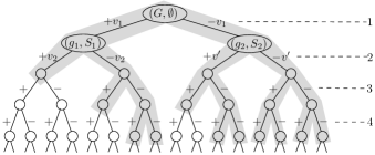
Figure 3. A snippet of the (binary) search tree $\cal T$ of a backtracking algorithm

The state-of-the-art time complexity is achieved by $\mathsf{kDC}$ (Chang, 2023) which proposes a new branching rule and two reduction rules to achieve the time complexity. Specifically, $\mathsf{kDC}$ proposes the non-fully-adjacent-first branching rule BR preferring branching on a vertex that is not fully adjacent to $S$, and the excess-removal reduction rule RR1 and the high-degree reduction rule RR2.

BR (Chang, 2023).:

Given an instance $(g,S)$, the branching vertex is selected as the vertex of $V(g)\setminus S$ that has at least one non-neighbor in $S$; if no such vertices exist, an arbitrary vertex of $V(g)\setminus S$ is chosen as the branching vertex.

RR1 (Chang, 2023).:

Given an instance $(g,S)$, if a vertex $u\in V(g)\setminus S$ satisfies $|\overline{E}(S\cup u)|>k$, we can remove $u$ from $g$.

RR2 (Chang, 2023).:

Given an instance $(g,S)$, if a vertex $u\in V(g)\setminus S$ satisfies $|\overline{E}(S\cup u)|\leq k$ and $d_{g}(u)\geq|V(g)|-2$, we can greedily add $u$ to $S$.

3.2. Time Complexity Analysis of $\mathsf{kDC}$

The general idea of time complexity analysis is as follows. As polynomial factors are usually ignored in the time complexity analysis of exponential time algorithms, it is sufficient to bound the number of leaf nodes of the search tree (in Figure 3) inductively in a bottom-up fashion (Fomin and Kratsch, 2010). One way of bounding the number of leaf nodes of the subtree rooted at the node corresponding to instance $(g,S)$ is to order $V(g)\setminus S$ in such a way that the longest prefix of the ordering that can be added to $S$ without violating the $k$-defective clique definition is short and bounded. Specifically, let $(v_{1},\ldots,v_{l},v_{l+1},\ldots)$ be an ordering of $V(g)\setminus S$ such that the longest prefix that can be added to $S$ without violating the $k$-defective clique definition is $(v_{1},\ldots,v_{l})$; that is, $\{v_{1},\ldots,v_{l},v_{l+1}\}\cup S$ induces more than $k$ non-edges. Then, we only need to generate $l+1$ new instances/branches, corresponding to the first $l+1$ prefixes, as shown in Figure 4: for the $i$-th (starting from $0$) branch, we include $(v_{1},\ldots,v_{i})$ to $S$ and remove $v_{i+1}$ from $g$. Denote the $i$-th branch by $(g_{i},S_{i})$. It holds that

• $|V(g_{i})\setminus S_{i}|\leq|V(g)\setminus S|-(i+1),\forall 0\leq i\leq l$.

It can be shown by the techniques of (Fomin and Kratsch, 2010) that the number of leaf nodes of the search tree is at most $\gamma^{n}$ where $\gamma<2$ is the largest real root of the equation $x^{l_{\max}+2}-2x^{l_{\max}+1}+1=0$ and $l_{\max}$ is the largest $l$ among all non-leaf nodes. Thus, the smaller the value of $l_{\max}$, the better the time complexity.

Figure 4. General idea of time complexity analysis

For $\mathsf{kDC}$, $l_{\max}=k+1$ and thus its time complexity is ${\cal O}^{*}(\gamma_{k}^{n})$ where $\gamma_{k}<2$ is the largest real root of the equation $x^{k+3}-2x^{k+2}+1=0$ (Chang, 2023); here, the ${\cal O}^{*}$ notation hides polynomial factors. Specifically, $\mathsf{kDC}$ orders $V(g)\setminus S$ by iteratively applying BR. That is, each time it appends to the ordering a vertex that has at least one non-neighbor in either $S$ or the vertices already in the ordering; if no such vertices exist, an arbitrary vertex of $V(g)\setminus S$ is appended. It is proved in (Chang, 2023) that after exhaustively applying reduction rules RR1 and RR2, the resulting instance $(g,S)$ satisfies the condition:

• $|\overline{E}(S\cup u)|\leq k$ and $d_{g}(u)<|V(g)|-2$, $\forall u\in V(g)\setminus S$.

i.e., every vertex of $V(g)\setminus S$ has at least two non-neighbors in $g$. Then, the worst-case scenario (for time complexity) is that the non-edges of $g[V(g)\setminus S]$ form a set of vertex-disjoint cycles; a length-$(k+1)$ prefix of the ordering induces exactly $k$ non-edges, and a length-$(k+2)$ prefix induces more than $k$ non-edges.

One may notice that Figure 3 illustrates a binary search tree while Figure 4 shows a multi-way search tree. Nevertheless, the above techniques can be used to analyze Figure 3 since a binary search tree can be (virtually) converted into an equivalent multi-way search tree, which is the way the time complexity of $\mathsf{kDC}$ was analyzed in (Chang, 2023). That is, we could collapse a length-$l$ path in Figure 3 to make it have $l+1$ children. This will be more clear when we conduct our time complexity analysis in Lemma 4.4.

3.3. Challenges of Improving the Time Complexity

As discussed in Section 3.2, the smaller the value of $l_{\max}$, the better the time complexity. $\mathsf{kDC}$ (Chang, 2023) proves that $l_{\max}\leq k+1$ by making all vertices of $V(g)\setminus S$ have at least two non-neighbors in $g$, which is achieved by RR2. In contrast, if all vertices of $V(g)\setminus S$ have exactly one non-neighbor in $g$, then $l_{\max}$ becomes $2k+1$ and the time complexity is ${\cal O}^{*}(\gamma_{2k}^{n})$, which is the case of $\mathsf{MADEC^{+}}$ (Chen et al., 2021).

It is natural to wonder whether the value of $l_{\max}$ can be reduced if we have techniques to make each vertex of $V(g)\setminus S$ have more (than two) non-neighbors in $g$. Specifically, let’s consider the complement graph $\overline{g}$ of $g$: each edge of $\overline{g}$ corresponds to a non-edge of $g$. The question is whether the BR of $\mathsf{kDC}$ can guarantee $l_{\max}<k+1$ when $\overline{g}[V(g)\setminus S]$ has a minimum degree larger than two. Unfortunately, the answer is negative. It is shown in (Sachs, 1963) that for any $r\geq 2$ and $s\geq 3$, there exists a graph in which each vertex has exactly $r$ neighbors and the shortest cycle has length exactly $s$; these graphs are called $(r,s)$-graphs. Thus, when $\overline{g}[V(g)\setminus S]$ is an $(r,s)$-graph for $s\geq k+2$, iteratively applying the branching rule BR may first identify vertices of the shortest cycle and it then needs a prefix of length $k+2$ to cover $k+1$ edges of $\overline{g}[V(g)\setminus S]$ (corresponding to $k+1$ non-edges of $g$). Alternatively, one may tempt to design a different branching rule than BR for finding a subset of $k+1$ or fewer vertices $C\subseteq V(g)\setminus S$ such that $\overline{g}[C]$ has at least $k+1$ edges. This most likely cannot be conducted efficiently, by noting that it is NP-hard to find a densest $k$-subgraph (i.e., a subgraph with exactly $k$ vertices and the most number of edges) when $k$ is a part of the input (Feige et al., 2001).

4. Our Algorithm with Improved Time Complexity

Despite the challenges and negative results mentioned in Section 3.3, we in this section show that we can reduce both the base and the exponent of the time complexity. In the following, we first present our algorithm in Section 4.1, then analyze its time complexity in Section 4.2, and finally analyze the time complexity again but using the degeneracy gap parameterization in Section 4.3.

4.1. Our Algorithm $\mathsf{kDC\text{-}two}$

Our algorithm uses the same branching rule BR and reduction rules RR1 and RR2 as $\mathsf{kDC}$. But we will show in Section 4.2 that the base of the time complexity is reduced by using different analysis techniques for different nodes of the search tree. Furthermore, we make use of the diameter-two property of large $k$-defective cliques to reduce the exponent of the time complexity, by observing that most real graphs have $\omega_{k}(G)\geq k+2$.

Lemma 4.1 (Diameter-two Property of Large $k$-Defective Clique (Chen et al., 2021)).

For any $k$-defective clique, if it contains at least $k+2$ vertices, its diameter is at most two (i.e., any two non-adjacent vertices must have common neighbors in the defective clique).

Following Lemma 4.1, if we know that $\omega_{k}(G)\geq k+2$, then for a backtracking instance $(g,S)$ with $S\neq\emptyset$, we can remove from $g$ the vertices whose shortest distance (computed in $g$) to any vertex of $S$ is greater than two. This could significantly reduce the search space, as real graphs usually have a small average degree. However, it is difficult to utilize the diameter-two property reliably, since we do not know before-hand whether $\omega_{k}(G)\geq k+2$ or not and a $k$-defective clique of size smaller than $k+2$ may have a diameter larger than two. To resolve this, we propose to compute the maximum $k$-defective clique in two stages, where Stage-I utilizes the diameter-two property for pruning by assuming $\omega_{k}(G)\geq k+2$. If Stage-I fails (to find a $k$-defective clique of size at least $k+2$), then we go to Stage-II searching the graph again without utilizing the diameter-two property. This guarantees that the maximum $k$-defective clique is found regardless of its size.

Input: A graph $G$ and an integer $k$

Output: A maximum $k$-defective clique in $G$

1

2 $C^{*}\leftarrow\emptyset$;

3 Let $(v_{1},\dots,v_{n})$ be a degeneracy ordering of the vertices of $G$;

4 for each $v_{i}\in V(G)$ do

5       $A\leftarrow N(v_{i})\cap\{v_{i},\ldots,v_{n}\}$;

6       Let $g_{v_{i}}$ be the subgraph of $G$ induced by $N[A]\cap\{v_{i},\ldots,v_{n}\}$;

7       ${\mathsf{Branch\&Bound}}(g_{v_{i}},\{v_{i}\})$;

8      

9 end for

10if $|C^{*}|<k+1$ then ${\mathsf{Branch\&Bound}}(G,\emptyset)$;

11 return $C^{*}$;

12

Procedure ${\mathsf{Branch\&Bound}}(g,S)$

13 $(g^{\prime},S^{\prime})\leftarrow$ apply reduction rules RR1 and RR2 to $(g,S)$;

14 if $g^{\prime}$ is a $k$-defective clique then update $C^{*}$ by $V(g^{\prime})$ and return;

15 $b\leftarrow$ choose a branching vertex from $V(g^{\prime})\setminus S^{\prime}$ based on BR;

16 ${\mathsf{Branch\&Bound}}(g^{\prime},S^{\prime}\cup b)$; /* Left branch includes $b$ */;

17 ${\mathsf{Branch\&Bound}}(g^{\prime}\setminus b,S^{\prime})$; /* Right branch excludes $b$ */;

Algorithm 1 ${\mathsf{kDC\text{-}two}}(G,k)$

The pseudocode of our algorithm $\mathsf{kDC\text{-}two}$ is shown in Algorithm 1 which takes a graph $G$ and an integer $k$ as input and outputs a maximum $k$-defective clique of $G$; here, $\mathsf{two}$ refers to both “two”-stage and diameter-“two”. Let $C^{*}$ store the currently found largest $k$-defective clique, which is initialized as $\emptyset$ (Line 1). We first compute a degeneracy ordering of the vertices of $G$ (Line 2). Without loss of generality, let $(v_{1},\ldots,v_{n})$ be the degeneracy ordering, i.e., for each $1\leq i\leq n$, $v_{i}$ is the vertex with the smallest degree in the subgraph of $G$ induced by $\{v_{i},\ldots,v_{n}\}$; the degeneracy ordering can be computed in ${\cal O}(m)$ time by the peeling algorithm (Matula and Beck, 1983). Then, for each vertex $v_{i}\in V(G)$, we compute the largest diameter-two $k$-defective clique in which the first vertex, according to the degeneracy ordering, is $v_{i}$, by invoking the procedure ${\mathsf{Branch\&Bound}}$ with input $(g_{v_{i}},\{v_{i}\})$ (Lines 4–6); that is, the diameter-two $k$-defective clique contains $v_{i}$ and is a subset of $(v_{i},v_{i+1},\ldots,v_{n})$. Here, $g_{v_{i}}$ is the subgraph of $G$ induced by $v_{i}$ and its neighbors and two-hop neighbors that come later than $v_{i}$ according to the degeneracy ordering. After that, we check whether the currently found largest $k$-defective clique $C^{*}$ is of size at least $k+1$: if $|C^{*}|\geq k+1$, then $C^{*}$ is guaranteed to be a maximum $k$-defective clique of $G$; otherwise, $\omega_{k}(G)\leq k+1$ and the maximum $k$-defective clique of $G$ may have a diameter larger than two. For the latter, we invoke $\mathsf{Branch\&Bound}$ again with input $(G,\emptyset)$ (Line 7). Note that, we do not make use of the diameter-two property for pruning within the procedure $\mathsf{Branch\&Bound}$, and thus ensure the correctness of our algorithm.

The pseudocode of the procedure ${\mathsf{Branch\&Bound}}$ is shown at Lines 9–13 of Algorithm 1. Given an input $(g,S)$, we first apply reduction rules RR1 and RR2 to reduce the instance $(g,S)$ to a potentially smaller instance $(g^{\prime},S^{\prime})$ such that $V(g^{\prime})\setminus S^{\prime}\subseteq V(g)\setminus S$ (Line 9). If $g^{\prime}$ itself is a $k$-defective clique, then we update $C^{*}$ by $V(g^{\prime})$ and backtrack (Line 10). Otherwise, we pick a branching vertex $b$ based on the branching rule BR (Line 11), and generate two $\mathsf{Branch\&Bound}$ instances and go into recursion (Lines 12–13).

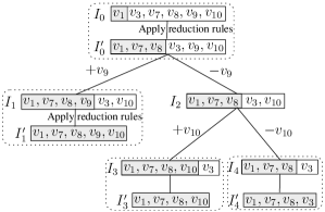
Figure 5. Running example

Example 4.2.

Consider the graph $G$ in Figure 2. $(v_{1},v_{2},\ldots,v_{14})$ is a degeneracy ordering of $G$; for example, $v_{1}$ has the smallest degree in $G$, and after removing $v_{1}$, $v_{2}$ then has the smallest degree, so on so forth. When processing $v_{1}$, we only need to consider its neighbors $\{v_{7},v_{8}\}$ and two-hop neighbors $\{v_{3},v_{9},v_{10}\}$; that is, we only need to consider the subgraph $g_{v_{1}}$ that is induced by $\{v_{1},v_{3},v_{7},\ldots,v_{10}\}$. The backtracking search tree for ${\mathsf{Branch\&Bound}}(g_{v_{1}},\{v_{1}\})$ is shown in Figure 5, where vertices of $S$ for each instance $(g,S)$ are in the shaded area. For the root node $I_{0}$, applying reduction rule RR2 adds $v_{7}$ and $v_{8}$ into $S$ since each of them has at most one non-neighbor in the subgraph; this results into the instance $I^{\prime}_{0}$. Suppose the branching rule BR selects $v_{9}$ for $I^{\prime}_{0}$ as $v_{9}$ is not adjacent to $v_{1}$. Then, two new instances $I_{1}$ and $I_{2}$ are generated as the two children of $I^{\prime}_{0}$. For $I_{1}$, applying the reduction rule RR1 removes $v_{3}$ from the graph and then applying RR2 adds $v_{10}$ into $S$; consequently we reach a leaf node. Similarly, $v_{10}$ is selected as the branching vertex for $I_{2}$, which then generates two leaf nodes $I^{\prime}_{3}$ and $I^{\prime}_{4}$.

4.2. Time Complexity Analysis of $\mathsf{kDC\text{-}two}$

To analyze the time complexity of $\mathsf{kDC\text{-}two}$, we use the same terminologies and notations as (Chang, 2023) and consider the search tree $\cal T$ of (recursively) invoking $\mathsf{Branch\&Bound}$ at either Line 6 or Line 7 of Algorithm 1, as shown in Figure 3. To avoid confusion, nodes of the search tree are referred to by nodes, and vertices of a graph by vertices. Nodes of $\cal T$ are denoted by $I,I^{\prime},I_{0},I_{1},\ldots$, and the graph $g$ and the partial solution $S$ of the $\mathsf{Branch\&Bound}$ instance to which $I$ corresponds are, respectively, denoted by $I.g$ and $I.S$. Note that $I.g$ and $I.S$ denote the ones obtained after applying the reduction rules at Lines 9–10 of Algorithm 1, where Line 10 is regarded as applying the reduction rule that if $g^{\prime}$ is a $k$-defective clique, then all vertices of $V(g^{\prime})\setminus S^{\prime}$ are added to $S^{\prime}$; that is, $I_{0},I_{1},I_{3},I_{4}$ in Figure 5 are instances before applying the reduction rules and could be discarded from the search tree. The size of $I$ is measured by the number of vertices of $I.g$ that are not in $I.S$, i.e., $|I|=|V(I.g)|-|I.S|=|V(I.g)\setminus I.S|$. It is worth mentioning that

• $|I^{\prime}|\leq|I|-1$ whenever $I^{\prime}$ is a child of $I$, e.g., the branching vertex $b$ of $I$ is in $V(I.g)\setminus I.S$ but not in $V(I^{\prime}.g)\setminus I^{\prime}.S$.

• $|I|=0$ whenever $I$ is a leaf node

For a non-leaf node $I_{0}$, we consider the path $(I_{0},I_{1},\ldots,I_{q})$ that starts from $I_{0}$, always visits the left child, and stops at $I_{q}$ once $q\geq 1$ and $|V(g_{q})|<|V(g_{q-1})|$; see Figure 6 for an example. Note that, the path is well defined since $I_{0}$ is a non-leaf node and thus $I_{0}.g$ is not a $k$-defective clique. For presentation simplicity, we abbreviate $I_{i}.g$ and $I_{i}.S$ as $g_{i}$ and $S_{i}$, respectively, and denote the branching vertex selected for $I_{i}$ by $b_{i}$. Let $u$ be an arbitrary vertex of $V(g_{q-1})\setminus V(g_{q})$. Then, $(b_{0},\ldots,b_{q-1},u,\ldots)$ is an ordering of $V(g_{0})\setminus S_{0}$ such that adding $(b_{0},\ldots,b_{q-1},u)$ to $S_{0}$ violates the $k$-defective clique definition. In the lemma below, we prove that $q\leq k$ if $I_{0}$ has at least one branching vertex being added.

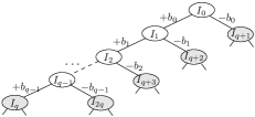
Figure 6. A left-deep walk in the search tree $\cal T$ starting from $I_{0}$; $I_{q}$ is the first node such that $q\geq 1$ and $|V(g_{q})|<|V(g_{q-1})|$

Lemma 4.3.

If the non-leaf node $I_{0}$ has at least one branching vertex being added, then $q\leq k$.

Proof.

Let $I_{x}$ be the last node, on the path $(I_{0},I_{1},\ldots,I_{x},\ldots,I_{q-1})$, satisfying the condition that all vertices of $V(g_{x})\setminus S_{x}$ are adjacent to all vertices of $S_{x}$, i.e., the branching vertex $b_{x}$ selected for $I_{x}$ has no non-neighbors in $S_{x}$. If such an $I_{x}$ does not exist, then we have $|\overline{E}(S_{i+1})|\geq|\overline{E}(S_{i})|+1$ for all $0\leq i<q$ (because the branching vertex added to $S_{i+1}$ must bring at least one non-edge to $\overline{E}(S_{i+1})$), and consequently $q\leq|\overline{E}(S_{q})|\leq k$. In the following, we assume that such an $I_{x}$ exists, and prove that $|\overline{E}(S_{x})|>x$ by considering two cases. Note that, each of the branching vertices $b_{i}\in\{b_{0},\dots,b_{x-1}\}$ that are added to $S_{x}$ must have at least two non-neighbors in $g_{i}$ (because of RR2) and all these non-neighbors are in $S_{x}$ (according to the definitions of $I_{x}$ and $I_{q}$).

• Case-I: $|\overline{E}(S_{0})|\neq 0$. Then, the number of unique non-edges associated with $\{b_{0},\ldots,b_{x-1}\}$ is at least $x$, and $|\overline{E}(S_{x})|\geq|\overline{E}(S_{0})|+x>x$.

• Case-II: $|\overline{E}(S_{0})|=0$. Let $b_{-1}$ be the branching vertex added to $S_{0}$ from its parent (which exists according to the lemma statement). Then, $b_{-1}$ has at least two non-neighbors in $g_{0}$; note that these non-neighbors will not be removed from $g_{0}$ by RR1 since $|\overline{E}(S_{0})|=0$ and all vertices of $V(g_{0})\setminus S_{0}$ are fully adjacent to vertices of $S_{0}\setminus b_{-1}$. Thus, the number of non-edges between $\{b_{-1},b_{0},\ldots,b_{x-1}\}$ is at least $x+1$, and hence $|\overline{E}(S_{x})|>x$.

Then, according to the definition of $I_{x}$ and our branching rule, for each $i$ with $x+1\leq i<q$, the branching vertex $b_{i}$ selected for $I_{i}$ has at least one non-neighbor in $S_{i}$, and consequently,

$$|\overline{E}(S_{q})|\geq|\overline{E}(S_{x})|+(q-x-1)>q-1$$

Thus, the lemma follows from the fact that $|\overline{E}(S_{q})|\leq k$. ∎

Let $\ell_{\cal T}(I)$ denote the number of leaf nodes in the subtree of $\cal T$ rooted at $I$. We prove in the lemma below that $\ell_{\cal T}(I)\leq\beta_{k}^{|I|}$ when at least one branching vertex has been added to $I$. Note that $\beta_{k}=\gamma_{k-1}$.

Lemma 4.4.

For any node $I$ of $\cal T$ that has at least one branching vertex being added, it holds that $\ell_{\cal T}(I)\leq\beta_{k}^{|I|}$ where $1<\beta_{k}<2$ is the largest real root of the equation $x^{k+2}-2x^{k+1}+1=0$.

Proof.

We prove the lemma by induction. For the base case that $I$ is a leaf node, it is trivial that $\ell_{\cal T}(I)=1\leq\beta_{k}^{|I|}$ since $\beta_{k}>1$ and $|I|=0$. For a non-leaf node $I_{0}$, let’s consider the path $(I_{0},I_{1},\ldots,I_{q^{\prime}})$ that starts from $I_{0}$, always visits the left child in the search tree $\cal T$, and stops at $I_{q^{\prime}}$ once $q^{\prime}\geq 1$ and $|I_{q^{\prime}}|\leq|I_{q^{\prime}-1}|-2$. Note that $(I_{0},\ldots,I_{q^{\prime}})$ is a prefix of $(I_{0},\ldots,I_{q})$ since $I_{q}$ satisfies the condition that $q\geq 1$ and $|I_{q}|\leq|I_{q-1}|-2$. It is trivial that

$$\ell_{\cal T}(I_{0})=\ell_{\cal T}(I_{q^{\prime}})+\ell_{\cal T}(I_{q^{\prime}+1})+\ell_{\cal T}(I_{q^{\prime}+2})+\cdots+\ell_{\cal T}(I_{2q^{\prime}})$$

where $I_{q^{\prime}+1},I_{q^{\prime}+2},\ldots,I_{2q^{\prime}}$ are the right child of $I_{0},I_{1},\ldots,I_{q^{\prime}-1}$, respectively, as illustrated in Figure 6 (by replacing $q$ with $q^{\prime}$); this is equivalent to converting a binary search tree to a multi-way search tree by collapsing the path $(I_{0},\ldots,I_{q^{\prime}-1})$ into a super-node that has $I_{q^{\prime}},I_{q^{\prime}+1},\ldots,I_{2q^{\prime}}$ as its children. To bound $\ell_{\cal T}(I_{0})$, we need to bound $q^{\prime}$ and $|I_{i}|$ for $q^{\prime}\leq i\leq 2q^{\prime}$. Following from Lemma 4.3, we have

Fact 1.:

$q^{\prime}\leq q\leq k$.

Also, according to the definition of the path, it holds that

(1) $$\forall i\in[1,q^{\prime}-1],\quad S_{i}=S_{i-1}\cup b_{i-1},\quad V(g_{i})=V(g_{i-1})$$

That is, the reduction rules at Line 9 of Algorithm 1 have no effect on $I_{i}$ for $1\leq i<q^{\prime}$. Then, the following two facts hold.

Fact 2.:

$\forall i\in[q^{\prime}+1,2q^{\prime}]$, $|I_{i}|\leq|I_{i-q^{\prime}-1}|-1\leq|I_{0}|+q^{\prime}-i$.

Fact 3.:

$|I_{q^{\prime}}|\leq|I_{q^{\prime}-1}|-2\leq|I_{0}|-q^{\prime}-1$.

Based on Facts 1, 2 and 3, we have

$$\ell_{\cal T}(I_{0}) =\ell_{\cal T}(I_{q^{\prime}+1})+\ell_{\cal T}(I_{q^{\prime}+2})+\cdots+\ell_{\cal T}(I_{2q^{\prime}})+\ell_{\cal T}(I_{q^{\prime}})$$

$$\leq\beta_{k}^{|I_{q^{\prime}+1}|}+\beta_{k}^{|I_{q^{\prime}+2}|}+\cdots+\beta_{k}^{|I_{2q^{\prime}}|}+\beta_{k}^{|I_{q^{\prime}}|}$$

$$\leq\beta_{k}^{|I_{0}|-1}+\beta_{k}^{|I_{0}|-2}+\cdots+\beta_{k}^{|I_{0}|-q^{\prime}}+\beta_{k}^{|I_{0}|-q^{\prime}-1}$$

$$\leq\beta_{k}^{|I_{0}|-1}+\beta_{k}^{|I_{0}|-2}+\cdots+\beta_{k}^{|I_{0}|-k}+\beta_{k}^{|I_{0}|-k-1}$$

where $\beta_{k}^{|I_{0}|-1}+\beta_{k}^{|I_{0}|-2}+\cdots+\beta_{k}^{|I_{0}|-k}+\beta_{k}^{|I_{0}|-k-1}\leq\beta_{k}^{|I_{0}|}$ if $\beta_{k}$ is no smaller than the largest real root of the equation $x^{k+1}-x^{k}-\cdots-x-1=0$ which is equivalent to the equation $x^{k+2}-2x^{k+1}+1=0$ (Fomin and Kratsch, 2010). The first few solutions to the equation are $\beta_{1}=1.619$, $\beta_{2}=1.840$, $\beta_{3}=1.928$, $\beta_{4}=1.966$, and $\beta_{5}=1.984$. ∎

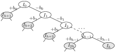
Figure 7. A right-deep walk in the search tree $\cal T$ starting from $I_{0}$ and stopping at a leaf node $I_{h}$

In Lemma 4.4, we cannot bound $\ell_{\cal T}(I)$ by $\beta_{k}^{|I|}$ if no branching vertices have been added to $I$. Nevertheless, we prove in the lemma below that $\ell_{\cal T}(I)<2\cdot\beta_{k}^{|I|}$ holds for every node $I$ of $\cal T$, by using a non-inductive proving technique.

Lemma 4.5.

For any node $I$ of $\cal T$, it holds that $\ell_{\cal T}(I)<2\cdot\beta_{k}^{|I|}$.

Proof.

If $I$ is a leaf node, the lemma is trivial. For a non-leaf node $I_{0}$, let’s consider the path $(I_{0},I_{1},\ldots,I_{h})$ that starts from $I_{0}$, always visits the right child in the search tree $\cal T$, and stops at a leaf node $I_{h}$; see Figure 7 for an example. Then, it holds that

$$\forall i\in[h+1,2h],|I_{i}|\leq|I_{i-h-1}|-1\leq|I_{0}|+h-i$$

and $|I_{h}|=0$. Moreover, for each $i\in[h+1,2h]$, $I_{i}$ has at least one branching vertex (e.g., $b_{i-h-1}$) being added, and thus according to Lemma 4.4, it satisfies $\ell_{\cal T}(I_{i})\leq\beta_{k}^{|I_{i}|}$. Consequently,

$$\ell_{\cal T}(I_{0}) =\ell_{\cal T}(I_{h+1})+\ell_{\cal T}(I_{h+2})+\cdots+\ell_{\cal T}(I_{2h})+\ell_{\cal T}(I_{h})$$

$$\leq\beta_{k}^{|I_{h+1}|}+\beta_{k}^{|I_{h+2}|}+\cdots+\beta_{k}^{|I_{2h}|}+\beta_{k}^{|I_{h}|}$$

$$\leq\beta_{k}^{|I_{0}|-1}+\beta_{k}^{|I_{0}|-2}+\cdots+\beta_{k}^{|I_{0}|-h}+1$$

$$\textstyle\leq\frac{\beta_{k}^{|I_{0}|}-1}{\beta_{k}-1}+1<2\cdot\beta_{k}^{|I_{0}|}$$

The last inequality follows from the fact that $\beta_{k}>1.5,\forall k\geq 1$. ∎

Following Lemma 4.5, Line 7 of Algorithm 1 runs in ${\cal O}^{*}(\beta_{k}^{n})$ time. What remains is to bound $|I|$ for Line 6 of Algorithm 1. Let $f$ denote the vertex obtained at Line 3 of Algorithm 1, $g$ be the subgraph extracted at Line 5, and $t$ be the number of $f$’s non-neighbors in $g$. It holds that $d_{g}(f)=|A|\leq\alpha$ since a degeneracy ordering is used for extracting $g$, $t\leq\alpha(\Delta-1)$, and $|V(g)|\leq d_{g}(f)+t+1\leq\alpha\Delta+1$; here, $\alpha$ is the degeneracy of $G$ and $\Delta$ is the maximum degree of $G$. We prove the time complexity of $\mathsf{kDC\text{-}two}$ in the theorem below.

Theorem 4.6.

Given a graph $G$ and an integer $k$, $\mathsf{kDC\text{-}two}$ runs in ${\cal O}(n\times(\alpha\Delta)^{2}\times\beta_{k}^{\alpha\Delta})$ time when $\omega_{k}(G)\geq k+2$, and in ${\cal O}(m\times\beta_{k}^{n})$ time otherwise.

Proof.

Each invocation of $\mathsf{Branch\&Bound}$ at Line 6 of Algorithm 1 takes ${\cal O}((\alpha\Delta)^{2}\times\beta_{k}^{\alpha\Delta})$ time, since the root node $I$ of the search tree satisfies $|I|\leq\alpha\Delta$ and each node of the search tree (i.e., Lines 9–11 of Algorithm 1) takes ${\cal O}(|E(g)|)={\cal O}((\alpha\Delta)^{2})$ time. When $\omega_{k}(G)\geq k+2$, the condition of Line 7 is not satisfied and thus Algorithm 1 runs in ${\cal O}(n\times(\alpha\Delta)^{2}\times\beta_{k}^{\alpha\Delta})$ time. Otherwise, Line 7 takes ${\cal O}(m\times\beta_{k}^{n})$ time and Algorithm 1 runs in ${\cal O}(n\times(\alpha\Delta)^{2}\times\beta_{k}^{\alpha\Delta}+m\times\beta_{k}^{n})$; for simplicity, we abbreviate this time complexity as ${\cal O}(m\times\beta_{k}^{n})$ since it is usually the dominating term. ∎

4.2.1. Further Reduce the Exponent

In the following, we show that when $\omega_{k}(G)\geq k+2$, the exponent of the time complexity can be further reduced by a more refined analysis. Let $I_{0}=(g_{0},S_{0})$ be the root of $\cal T$ for Line 6 of Algorithm 1; recall that, $f\in S_{0}$, $d_{g_{0}}(f)\leq d_{g}(f)\leq\alpha$ and $|I_{0}|\leq\alpha+t$, where $f$ is the vertex obtained at Line 3 of Algorithm 1 and $t$ is number of $f$’s non-neighbors in the subgraph $g$ extracted for $f$. Let’s consider the subtree of $\cal T$ formed by starting a depth-first-search from $I_{0}$ and backtracking once the path from $I_{0}$ to it has either $t$ total edges or $k$ positive edges (i.e., labeled as “+”); see the shaded subtree in Figure 3 for an illustration of $t=4$ and $k=2$. Let $\cal L$ be the set of leaf nodes of this subtree. Then, the number of leaf nodes of $\cal T$ satisfies

$$\ell_{\cal T}(I_{0})\leq\sum_{I\in\cal L}\ell_{\cal T}(I)$$

We bound $|\cal L|$ and $\ell_{\cal T}(I)$ for $I\in\cal L$ in the following two lemmas.

Lemma 4.7.

$|\cal L|={\cal O}(t^{k})$ where $t$ is the number of $f$’s non-neighbors in $g$.

Proof.

To bound $|\cal L|$, we observe that the search tree $\cal T$ is a full binary tree with each node having a positive edge to its left child and a negative edge to its right child. Thus, we can label every edge by its level in the tree (see Figure 3), and for each node $I\in\cal L$, we associate with it a set of numbers corresponding to the levels of the positive edges from $I_{0}$ to $I$. Then, it is easy to see that each node of $\cal L$ is associated with a distinct subset, of size at most $k$, of $\{1,2,\ldots,t\}$. Consequently, $|\cal L|\leq\sum_{i=0}^{k}{t\choose i}={\cal O}(t^{k})$ (Mohri et al., 2012). ∎

Lemma 4.8.

For all $I\in\cal L$, it holds that $|I|\leq\alpha$ and $|V(I.g)|\leq\alpha+k+1$.

Proof.

Let’s consider the path $(I_{0},I_{1},\ldots,I_{p-1},I_{p}=I)$ from $I_{0}$ to $I$. If there are $k$ positive edges on the path, then all vertices of $V(g_{p})\setminus S_{p}$ must be adjacent to $f$, and thus $|I_{p}|\leq\alpha$ and $|V(g_{p})|\leq\alpha+k+1$. The latter holds since all of $f$’s non-neighbors in $g$ are in $S$ and thus of quantity at most $k$. The former can be shown by contradiction. Suppose $V(g_{p})\setminus S_{p}$ contains a non-neighbor of $f$, then adding each of the $k$ branching vertices (on the positive edges of the path) must bring at least one non-edge to $S_{p}$, due to the branching rule BR; then RR1 will remove all non-neighbors of $f$ from $V(g_{p})\setminus S_{p}$, contradiction.

Otherwise, there are at most $k-1$ positive edges on the path and $p=t$. Then, $|I_{p}|\leq|I_{0}|-t\leq\alpha$. Also, there are at least $t-k+1$ negative edges on the path and thus $|V(g_{p})|\leq|V(g_{0})|-(t-k+1)\leq t+\alpha+1-(t-k+1)=\alpha+k$. ∎

Consequently, the number of leaf nodes of $\cal T$ is ${\cal O}((\alpha\Delta)^{k}\beta_{k}^{\alpha})$ and the time complexity of $\mathsf{kDC\text{-}two}$ follows.

Theorem 4.9.

Given a graph $G$ and an integer $k$, $\mathsf{kDC\text{-}two}$ runs in ${\cal O}(n\times(\alpha\Delta)^{k+2}\times\beta_{k}^{\alpha})$ time when $\omega_{k}(G)\geq k+2$.

4.2.2. Compared with $\mathsf{kDC}$

Our algorithm $\mathsf{kDC\text{-}two}$ improves the time complexity of $\mathsf{kDC}$ (Chang, 2023) from two aspects. Firstly, we improve the base of the exponential time complexity from $\gamma_{k}$ to $\beta_{k}=\gamma_{k-1}$. This is achieved by using different analysis techniques for the nodes that already have branching vertices being added (i.e., Lemma 4.4) and for those that do not (i.e., Lemma 4.5). Without this separation, we can only bound the length $q$ of the path $(I_{0},\ldots,I_{q})$ by $k+1$ instead of $k$ that is proved in Lemma 4.3. Also note that, Lemma 4.5 is non-inductive and has a coefficient $2$ in the bound; if we use induction in the proof of Lemma 4.5, then the coefficient will become bigger and bigger and become exponential when going up the tree. Secondly, we improve the exponent of the time complexity from $n$ to $\alpha$ when $\omega_{k}(G)\geq k+2$; note that, most real graphs have $\omega_{k}(G)\geq k+2$. This is achieved by our two-stage algorithm that utilizes the diameter-two property for pruning in Stage-I, as well as our refined analysis in Section 4.2.1.

4.3. Parameterize by the Degeneracy Gap

In this subsection, we prove that $\mathsf{kDC\text{-}two}$, with slight modification, runs in ${\cal O}^{*}((\alpha\Delta)^{k+2}(k+1)^{\alpha+k+1-\omega_{k}(G)})$ time by using the degeneracy gap $\alpha+k+1-\omega_{k}(G)$ parameterization; this is better than ${\cal O}^{*}((\alpha\Delta)^{k+2}\beta_{k}^{\alpha})$ when $\omega_{k}(G)$ is close to $\alpha+k+1$, the degeneracy-based upper bound of $\omega_{k}(G)$. Specifically, let’s consider the problem of testing whether $G$ has a $k$-defective clique of size $\tau$. To do so, we truncate the search tree $\cal T$ by cutting the entire subtree rooted at node $I$ if $|V(I.g)|\leq\tau$; that is, we terminate ${\mathsf{Branch\&Bound}}$ once $|V(g^{\prime})|\leq\tau$ after Line 10 of Algorithm 1. Let $\cal T^{\prime}$ be the truncated version of $\cal T$. We first bound the number of leaf nodes of $\cal T^{\prime}$ in the following two lemmas, in a similar fashion as Lemmas 4.4 and 4.5.

Lemma 4.10.

For any node $I$ of $\cal T^{\prime}$ that has at least one branching vertex being added, it holds that $\ell_{\cal T^{\prime}}(I)\leq(k+1)^{|V(I.g)|-\tau}$.

Proof.

We prove the lemma by induction. For the base case that $I$ is a leaf node, we have $|V(I.g)|=\tau$ and thus $\ell_{\cal T^{\prime}}(I)=(k+1)^{0}=(k+1)^{|V(I.g)|-\tau}$. For a non-leaf node $I_{0}$ that has at least one branching vertex being added, let’s consider the path $(I_{0},I_{1},\ldots,I_{q})$ that starts from $I_{0}$, always visits the left child in the search tree $\cal T^{\prime}$, and stops at $I_{q}$ once $q\geq 1$ and $|V(g_{q})|<|V(g_{q-1})|$; this is the same one as studied at the beginning of Section 4.2, see Figure 6. According to Lemma 4.3, we have $q\leq k$. It is trivial that

$$\forall i\in[q,2q],\quad|V(g_{i})|<|V(g_{0})|$$

where $I_{q+1},I_{q+2},\dots,I_{2q}$ are the right child of $I_{0},I_{1},\dots,I_{q-1}$, respectively, as illustrated in Figure 6. Thus,

$$\ell_{\cal T^{\prime}}(I_{0}) =\ell_{\cal T^{\prime}}(I_{q})+\ell_{\cal T^{\prime}}(I_{q+1})+\ell_{\cal T^{\prime}}(I_{q+2})+\dots+\ell_{\cal T^{\prime}}(I_{2q})$$

$$\leq(q+1)\cdot(k+1)^{|V(g_{0})|-1-\tau}\leq(k+1)^{|V(g_{0})|-\tau}$$

∎

Lemma 4.11.

For any node $I$ of $\cal T^{\prime}$, it holds that $\ell_{\cal T^{\prime}}(I)<2\cdot(k+1)^{|V(I.g)|-\tau}$.

Proof.

If $I$ is a leaf node, the lemma is trivial. For a non-leaf node $I_{0}$, let’s consider the path $(I_{0},I_{1},\ldots,I_{h})$ that starts from $I_{0}$, always visits the right child in the search tree $\cal T^{\prime}$, and stops at a leaf node $I_{h}$; see Figure 7 for an example. Then, it holds that

$$\forall i\in[h+1,2h],|V(g_{i})|\leq|V(g_{i-h-1})|\leq|V(g_{0})|+h+1-i$$

and $|V(g_{h})|\leq|V(g_{0})|-h\leq\tau$. Moreover, for each $i\in[h+1,2h]$, $I_{i}$ has at least one branching vertex (e.g., $b_{i-h-1}$) being added, and thus according to Lemma 4.10, it satisfies $\ell_{\cal T^{\prime}}(I_{i})\leq(k+1)^{|V(g_{i})|-\tau}\leq(k+1)^{|V(g_{0})|+h+1-i-\tau}$. Consequently,

$$\ell_{\cal T^{\prime}}(I_{0}) =\ell_{\cal T^{\prime}}(I_{h+1})+\ell_{\cal T^{\prime}}(I_{h+2})+\cdots+\ell_{\cal T^{\prime}}(I_{2h})+\ell_{\cal T^{\prime}}(I_{h})$$

$$\leq(k+1)^{|V(g_{0})|-\tau}+(k+1)^{|V(g_{0})|-1-\tau}+\cdots+(k+1)^{1}+1$$

$$\textstyle\leq\frac{(k+1)^{|V(g_{0})|+1-\tau}-1}{k+1-1}<2\cdot(k+1)^{|V(g_{0})|-\tau}$$

The last inequality follows from the fact that $k\geq 1$. ∎

Then, the following time complexity can be proved in a similar way to Theorem 4.9 but using Lemma 4.11 and Lemma 4.8.

Lemma 4.12.

Testing whether $G$ has a $k$-defective clique of size $\tau$ for $\tau\geq k+2$ takes ${\cal O}(n\times(\alpha\Delta)^{k+2}\times(k+1)^{\alpha+k+1-\omega_{k}(G)})$ time.

Finally, we can find the maximum $k$-defective clique by iteratively testing whether $G$ has a $k$-defective clique of size $\tau$ for $\tau=\{\alpha+k+1,\alpha+k,\ldots\}$. This will find the maximum $k$-defective clique and terminate after testing $\tau=\omega_{k}(G)$. Consequently, the following time complexity follows.

Theorem 4.13.

The maximum $k$-defective clique in $G$ can be found in ${\cal O}((\alpha+k+2-\omega_{k}(G))\times n\times(\alpha\Delta)^{k+2}\times(k+1)^{\alpha+k+1-\omega_{k}(G)})$ time when $\omega_{k}(G)\geq k+2$.

5. A New Reduction Rule

In this section, we propose a new reduction rule based on the degree-sequence-based upper bound UB that is proposed in (Gao et al., 2022), to further improve the practical performance of $\mathsf{kDC\text{-}two}$.

UB (Gao et al., 2022).:

Given an instance $(g,S)$, let $v_{1},v_{2},\ldots$ be an ordering of $V(g)\setminus S$ in non-decreasing order regarding their numbers of non-neighbors in $S$, i.e.$|\overline{N}_{S}(\cdot)|$. The maximum $k$-defective clique in the instance $(g,S)$ is of size at most $|S|$ plus the largest $i$ such that $\sum_{j=1}^{i}|\overline{N}_{S}(v_{j})|\leq k-|\overline{E}(S)|$.

Note that, different tie-breaking techniques for ordering the vertices lead to the same upper bound. Thus, an arbitrary tie-breaking technique can be used in UB.

Let $lb$ be the size of the currently found best solution. If an upper bound computed by UB for an instance $(g,S)$ is no larger than $lb$, then we can prune the instance. However, this way of first generating an instance and then try to prune it based on a computed upper bound is inefficient. To improve efficiency, we propose to remove $u\in V(g)\setminus S$ from $g$ if an upper bound of $(g,S\cup u)$ is no larger than $lb$. Note that, rather than computing the exact upper bound for $(g,S\cup u)$, we only need to test whether the upper bound is larger than $lb$ or not. The latter can be conducted more efficiently and without generating $(g,S\cup u)$; moreover, computation can be shared between the testing for different vertices of $V(g)\setminus S$.

Let $v_{1},v_{2},\ldots$ be an ordering of $V(g)\setminus(S\cup u)$ in non-decreasing order regarding $|\overline{N}_{S}(\cdot)|$, and $C$ be the set of vertices that have the same number of non-neighbors in $S$ as $v_{lb-|S|}$, i.e., $C=\{v_{i}\in V(g)\setminus(S\cup u)\mid|\overline{N}_{S}(v_{i})|=|\overline{N}_{S}(v_{lb-|S|})|\}$. Let $C_{1}$ and $C_{2}$ be a partitioning of $C$ according to their positions in the ordering, i.e., $C_{1}=C\cap\{v_{1},\ldots,v_{lb-|S|}\}$ and $C_{2}=C\setminus C_{1}$. Note that, both $C_{1}$ and $C_{2}$ contain consecutive vertices in the ordering, and $C_{2}$ could be empty. A visualization of the ordering and vertex sets is shown below, where $S\cup u$ and $lb-|S|$ are denoted by $R$ and $r$ for brevity.

$$\underbrace{S,u}_{\text{$R$}},\underbrace{v_{1},\ldots,v_{r-|C_{1}|}}_{\text{$D$}},\overbrace{\underbrace{v_{r-|C_{1}|+1},\ldots,v_{r}}_{\text{$C_{1}$}},\underbrace{v_{r+1},\ldots v_{r+|C_{2}|}}_{\text{$C_{2}$}}}^{\text{$C=\{v_{i}\in V(g)\setminus R\mid|\overline{N}_{S}(v_{i})|=|\overline{N}_{S}(v_{r})|\}$}},\ldots$$

We prove in the lemma below that the upper bound computed by UB for the instance $(g,S\cup u)$ is at most $lb$ if and only if

(2) $$|\overline{E}(S)|+\sum_{j=1}^{r}|\overline{N}_{S}(v_{j})|+|\overline{N}_{S\cup D}(u)|+\max\{|\overline{N}_{C_{1}}(u)|-|N_{C_{2}}(u)|,0\}>k$$

Lemma 5.1.

The upper bound computed by UB for the instance $(g,S\cup u)$ is at most $lb$ if and only if Equation (2) is satisfied.

Proof.

Let’s firstly simply the left-hand side (LHS) of Equation (2). Note that, $|\overline{N}_{S\cup D}(u)|=|\overline{N}_{S}(u)|+|\overline{N}_{D}(u)|$, $|\overline{E}(S)|+|\overline{N}_{S}(u)|=|\overline{E}(R)|$, and $\sum_{j=1}^{r-|C_{1}|}|\overline{N}_{S}(v_{j})|+|\overline{N}_{D}(u)|=\sum_{j=1}^{r-|C_{1}|}|\overline{N}_{R}(v_{j})|$. Let $a=|\overline{N}_{C_{1}}(u)|$ and $b=|N_{C_{2}}(u)|$. Then, Equation (2) is equivalent to

(3) $$|\overline{E}(R)|+\sum_{j=1}^{r-|C_{1}|}|\overline{N}_{R}(v_{j})|+\sum_{v_{j}\in C_{1}}|\overline{N}_{S}(v_{j})|+\max\{a-b,0\}>k$$

Let $w_{1},w_{2},\ldots$ be an ordering of $V(g)\setminus R$ in non-decreasing order regarding $|\overline{N}_{R}(\cdot)|$. Then, the upper bound computed by UB for the instance $(g,R)$ is at most $lb$ if and only if

(4) $$|\overline{E}(R)|+\sum_{j=1}^{r}|\overline{N}_{R}(w_{j})|>k$$

For every $v\in V(g)\setminus R$, if $(u,v)\in E$, then $|\overline{N}_{R}(v)|=|\overline{N}_{S}(v)|$; otherwise, $|\overline{N}_{R}(v)|=|\overline{N}_{S}(v)|+1$. According to the definition of $C$, for every $v\in D$, it holds that $|\overline{N}_{S}(v)|<|\overline{N}_{S}(v_{r-|C_{1}|+1})|$ and thus $|\overline{N}_{R}(v)|\leq|\overline{N}_{S}(v_{r-|C_{1}|+1})|\leq|\overline{N}_{R}(w_{r-|C_{1}|+1})|$. Consequently, we can assume $\{w_{1},\ldots,w_{r-|C_{1}|}\}=D$; note however that, the ordering may be different. Similarly, we can assume $\{w_{r-|C_{1}|+1},\ldots,w_{r}\}\subseteq C_{1}\cup C_{2}$. Then, we have

$$\text{LHS of Equation~{}(\ref{eq:eq1})}-\text{LHS of Equation~{}(\ref{eq:eq2})}$$

$$= \sum_{j=r-|C_{1}|+1}^{r}|\overline{N}_{S}(v_{j})|+\max\{a-b,0\}-\sum_{j=r-|C_{1}|+1}^{r}|\overline{N}_{R}(w_{j})|$$

$$= |C_{1}|\cdot|\overline{N}_{S}(v_{r})|+\max\{a-b,0\}-\sum_{j=r-|C_{1}|+1}^{r}|\overline{N}_{R}(w_{j})|$$

There are exactly $|C_{1}|-a+b$ vertices of $C_{1}\cup C_{2}$ satisfying $|\overline{N}_{R}(\cdot)|=|\overline{N}_{S}(v_{r})|$. Thus, if $a\leq b$, then there are $|C_{1}|-a+b\geq|C_{1}|$ vertices of $C_{1}\cup C_{2}$ with $|\overline{N}_{R}(\cdot)|=|\overline{N}_{S}(v_{r})|$ and $\sum_{j=r-|C_{1}|+1}^{r}|\overline{N}_{R}(w_{j})|=|C_{1}|\cdot|\overline{N}_{S}(v_{r})|$; otherwise, $\sum_{j=r-|C_{1}|+1}^{r}|\overline{N}_{R}(w_{j})|=|C_{1}|\cdot|\overline{N}_{S}(v_{r})|+a-b$. Therefore, the lemma holds. ∎

Based on the above discussions, we propose the following degree-sequence-based reduction rule RR3.

RR3 (degree-sequence-based reduction rule).:

Given an instance $(g,S)$ with $|S|<lb<|V(g)|$ and a vertex $u\in V(g)\setminus S$, we remove $u$ from $g$ if Equation (2) is satisfied.

1 Obtain $|\overline{E}(S)|$ and $|\overline{N}_{S}(v)|$ for each $v\in V(g)\setminus S$;

2 Let $u_{1},u_{2},\ldots$ be an ordering of $V(g)\setminus S$ in non-decreasing order regarding $|\overline{N}_{S}(\cdot)|$;

3 $X\leftarrow\emptyset$;

4 for $i\leftarrow 1\textbf{ to }|V(g)\setminus S|$ do

5       if $|X|+|V(g)\setminus S|-i<lb-|S|$ then return $(g[S],S)$;

6       Let $v_{1},v_{2},\ldots$ be the vertices of $X\cup\{u_{i+1},u_{i+2},\ldots\}$ in non-decreasing order regarding $|\overline{N}_{S}(\cdot)|$;

7       Obtain $|\overline{N}_{D}(u_{i})|$, $|\overline{N}_{C_{1}}(u_{i})|$ and $|N_{C_{2}}(u_{i})|$;

8       if Equation (2) is not satisfied then Append $u_{i}$ to the end of $X$;

9      

10 end for

11return $(g[X],S)$;

Algorithm 2 ${\mathsf{ApplyRR3}}(g,S,lb)$

Given an instance $(g,S)$, our pseudocode of efficiently applying RR3 for all vertices of $V(g)\setminus S$ is shown in Algorithm 2, which returns a reduced instance at either Line 5 or Line 9. We first obtain $|\overline{E}(S)|$ and $|\overline{N}_{S}(v)|$ for each $v\in V(g)\setminus S$ (Line 1), and then order vertices of $V(g)\setminus S$ in non-decreasing order regarding $|\overline{N}_{S}(\cdot)|$ (Line 2). Let $u_{1},u_{2},\ldots$ be the ordered vertices. We then process the vertices of $V(g)\setminus S$ one-by-one according to the sorted order (Line 4). When processing $u_{i}$, the vertices that we need to consider are the vertices that have not been processed yet (i.e., $\{u_{i+1},u_{i+2},\ldots\}$) and the subset of $\{u_{1},u_{2},\ldots,u_{i-1}\}$ that passed (i.e., not pruned) by the reduction rule; denote the latter subset by $X$. This means that $\{u_{1},\ldots,u_{i-1}\}\setminus X$ have already been removed from $g$ by the reduction rule. If the number of remaining vertices (i.e., $|X|+|V(g)\setminus S|-i$) is less than $r=lb-|S|$, then we remove all vertices of $V(g)\setminus S$ from $g$ by returning $(g[S],S)$ (Line 5). Otherwise, let $v_{1},v_{2},\ldots,v_{r},\ldots$ be the vertices of $X\cup\{u_{i+1},u_{i+2},\ldots\}$ in non-decreasing order regarding $|\overline{N}_{S}(\cdot)|$ (Line 6). We obtain $|\overline{N}_{D}(u_{i})|$, $|\overline{N}_{C_{1}}(u_{i})|$ and $|N_{C_{2}}(u_{i})|$ (Line 7), and remove $u_{i}$ from $g$ if Equation (2) is satisfied; otherwise, $u_{i}$ is not pruned and is appended to the end of $X$ (Line 8). Finally, Line 9 returns the reduced instance $(g[X],S)$.

Lemma 5.2.

Algorithm 2 runs in ${\cal O}(|E(g)|+k)$ time.

Proof.

Firstly, Lines 1–2 run in ${\cal O}(|E(g)|+k)$ time, where the sorting is conducted by counting sort. Secondly, Line 6 does not do anything; it is just a syntax sugar for relabeling the vertices. Thirdly, Line 7 can be conducted in ${\cal O}(|N_{g}(u_{i})|)$ time since $|\overline{N}_{D}(u_{i})|=|D|-|N_{D}(u_{i})|$ and $|\overline{N}_{C_{1}}(u_{i})|=|C_{1}|-|N_{C_{1}}(u_{i})|$; note that, as each of $D,C_{1},C_{2}$ spans at most two arrays (i.e., $X$ and $\{u_{i+1},\ldots\}$), we can easily get its size and boundary. Lastly, Line 8 can be checked in constant time by noting that $\sum_{j=1}^{r}|\overline{N}_{S}(v_{j})|$ can be obtained in constant time after storing the suffix sums of $|\overline{N}_{S}(u_{1})|,|\overline{N}_{S}(u_{2})|,\ldots$, $|\overline{N}_{S}(u_{i+1})|,|\overline{N}_{S}(u_{i+2})|,\ldots$. ∎

Figure 8. Example instance for applying reduction rule RR3

Example 5.3.

Consider the instance $(g,S)$ in Figure 8 for $k=3$ and $lb=5$, where $g$ is the entire graph and $S=\{s_{1},s_{2},s_{3}\}$; thus $r=2$. The values of $|\overline{N}_{S}(\cdot)|$ for the vertices of $V(g)\setminus S=\{u_{1},\ldots,u_{5}\}$ are $\{u_{1}:0,u_{2}:0,u_{3}:1,u_{4}:1,u_{5}:1\}$. As $|\overline{E}(S)|=2$, the upper bound of $(g,S)$ computed by UB is $6$; thus, the instance is not pruned.

Let’s apply RR3 for $u_{1}$. As $X=\emptyset$, we have $v_{i}=u_{i+1}$ for $1\leq i\leq 4$. Then $D=\{u_{2}\},C_{1}=\{u_{3}\},C_{2}=\{u_{4},u_{5}\}$, $\sum_{j=1}^{r}|\overline{N}_{S}(v_{j})|=1$, $|\overline{N}_{S\cup D}(u_{1})|=0$, $|\overline{N}_{C_{1}}(u_{1})|=1$ and $|N_{C_{2}}(u_{1})|=1$. Thus, Equation (2) is not satisfied; $u_{1}$ is not pruned and is appended to $X$.

Now let’s apply RR3 for $u_{2}$. As $X=\{u_{1}\}$, we have $v_{1}=u_{1}$ and $v_{i}=u_{i+1}$ for $2\leq i\leq 4$. Then $D=\{u_{1}\},C_{1}=\{u_{3}\},C_{2}=\{u_{4},u_{5}\}$, $\sum_{j=1}^{r}|\overline{N}_{S}(v_{j})|=1$, $|\overline{N}_{S\cup D}(u_{2})|=0$, $|\overline{N}_{C_{1}}(u_{2})|=1$ and $|N_{C_{2}}(u_{2})|=0$. Consequently, Equation (2) is satisfied and $u_{2}$ is removed from $g$. It can be verified that $u_{3},u_{4},u_{5}$ will all subsequently be removed.

Effectiveness of RR3. $\mathsf{kDC}$ (Chang, 2023) also proposed a reduction rule based on UB; let’s denote it as RR3’. We remark that our RR3 is more effective (i.e., prunes more vertices) than RR3’ since the latter ignores the non-edges between $u$ and $V(g)\setminus(S\cup u)$ that are considered by RR3; specifically, RR3’ removes $u$ from $g$ if $|\overline{E}(S)|+\sum_{j=1}^{r}|\overline{N}_{S}(v_{j})|+|\overline{N}_{S}(u)|>k$. More generally, the effectiveness of our RR3 is characterized by the lemma below.

Lemma 5.4.

RR3 is more effective than any other reduction rule that is designed based on an upper bound of $(g,S\cup u)$ that ignores all the non-edges between vertices of $V(g)\setminus(S\cup u)$.

Proof.

Firstly, we have proved in Lemma 5.1 that applying RR3 is equivalent to computing UB for $(g,S\cup u)$. Secondly, it can be shown that UB computes the tightest upper bound for $(g,S\cup u)$ among all upper bounds that ignore all the non-edges between vertices of $V(g)\setminus(S\cup u)$. Thus, the lemma holds. ∎

In particular, the second-order reduction rule proposed in (Chang, 2023) is designed based on an upper bound of $(g,S\cup u)$ that does not consider the non-edges between vertices of $V(g)\setminus(S\cup u)$. Thus, RR3 is more effective than the second-order reduction rule of (Chang, 2023).

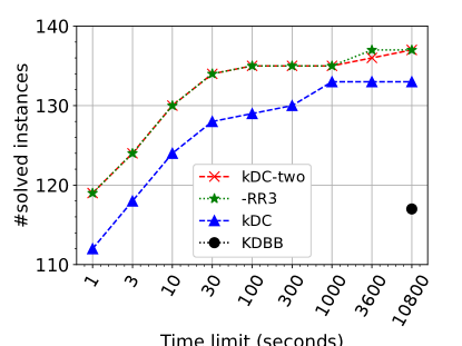
(a) $k=1$

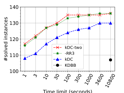
(b) $k=3$

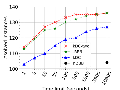
(c) $k=5$

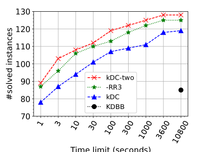
(d) $k=10$

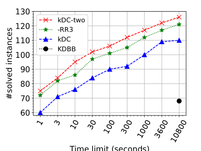
(e) $k=15$

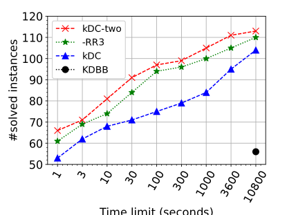
(f) $k=20$

Figure 9. Number of solved instances by varying time limit for real-world graphs (best viewed in color)

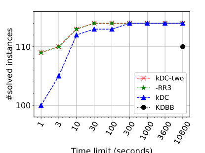
(a) $k=1$

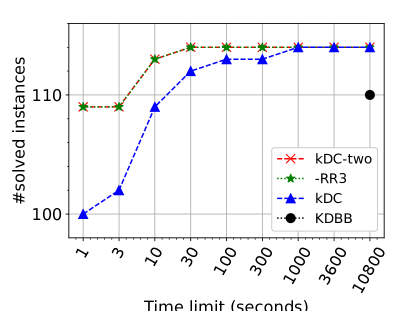
(b) $k=3$

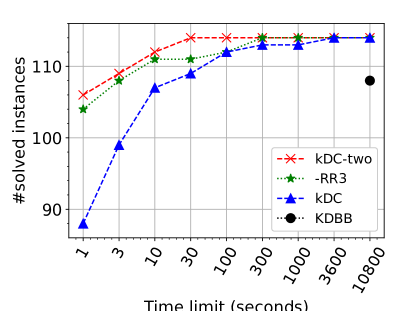
(c) $k=5$

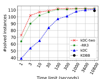
(d) $k=10$

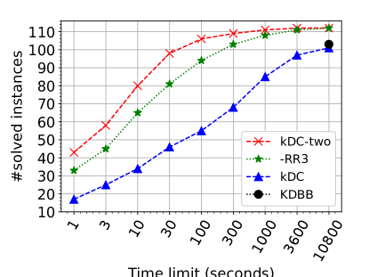
(e) $k=15$

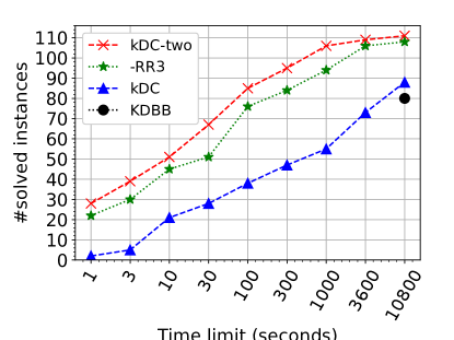
(f) $k=20$

Figure 10. Number of solved instances by varying time limit for Facebook graphs (best viewed in color)

6. Experiments

In this section, we evaluate the practical performance of $\mathsf{kDC\text{-}two}$, by comparing it against the following two existing algorithms.

• $\mathsf{kDC}$: the state-of-the-art algorithm proposed in (Chang, 2023).

• $\mathsf{KDBB}$: the existing algorithm proposed in (Gao et al., 2022).

We implemented our algorithm $\mathsf{kDC\text{-}two}$ based on the code-base of $\mathsf{kDC}$ that is downloaded from https://lijunchang.github.io/Maximum-kDC/; thus, all optimizations/techniques that are implemented in $\mathsf{kDC}$, except the second-order reduction rule, are used in $\mathsf{kDC\text{-}two}$. In addition, we also implemented the following variant of $\mathsf{kDC\text{-}two}$ to evaluate the effectiveness of our new reduction rule RR3.

• $\mathsf{\text{-}RR3}$: $\mathsf{kDC\text{-}two}$ without the reduction rule RR3.

All algorithms are implemented in C++ and compiled with the -O3 flag. All experiments are conducted in single-thread modes on a machine with an Intel Core i7-8700 CPU and 64GB main memory.

We run the algorithms on the following three graph collections, which are the same ones tested in (Gao et al., 2022; Chang, 2023).

• The real-world graphs collection  contains $139$ real-world graphs from the Network Data Repository with up to $5.87\times 10^{7}$ vertices and $1.06\times 10^{8}$ edges.

• The Facebook graphs collection  contains $114$ Facebook social networks from the Network Data Repository with up to $5.92\times 10^{7}$ vertices and $9.25\times 10^{7}$ edges.

• The DIMACS10&SNAP graphs collection contains 37 graphs with up to $1.04\times 10^{6}$ vertices and $6.89\times 10^{6}$ edges. $27$ of them are from DIMACS10  and $10$ graphs are from SNAP .

Same as (Gao et al., 2022; Chang, 2023), we choose $k$ from $\{1,3,5,10,15,20\}$, and set a time limit of $3$ hours for each testing (i.e., running a particular algorithm on a specific graph with a chosen $k$ value).

6.1. Against the Existing Algorithms

In this subsection, we evaluate the efficiency of our algorithm $\mathsf{kDC\text{-}two}$ against the existing algorithms $\mathsf{kDC}$ and $\mathsf{KDBB}$. Note that, (1) $\mathsf{kDC}$ is the fastest existing algorithm, and (2) as the code of $\mathsf{KDBB}$ is not available, the results of $\mathsf{KDBB}$ reported in this subsection are obtained from the original paper of $\mathsf{KDBB}$ (Gao et al., 2022).

Table 2. Number of instances solved by the algorithms $\mathsf{kDC\text{-}two}$, $\mathsf{kDC}$ and $\mathsf{KDBB}$ with a time limit of $3$ hours (best performers are highlighted in bold)

	Real-world graphs			Facebook graphs			DIMACS10&SNAP
	$\mathsf{kDC\text{-}two}$	$\mathsf{kDC}$	$\mathsf{KDBB}$	$\mathsf{kDC\text{-}two}$	$\mathsf{kDC}$	$\mathsf{KDBB}$	$\mathsf{kDC\text{-}two}$	$\mathsf{kDC}$	$\mathsf{KDBB}$
$k=1$	137	133	117	114	114	110	37	37	36
$k=3$	136	130	107	114	114	110	37	37	35
$k=5$	136	127	104	114	114	108	37	37	34
$k=10$	128	119	85	112	111	109	36	36	30
$k=15$	126	110	68	112	101	103	36	29	25
$k=20$	113	104	56	111	88	80	34	27	22

We first report in Table 2 the total number of graph instances that are solved by each algorithm with a time limit of 3 hours. We can see that for all three algorithms, the number of solved instances decreases when $k$ increases; this indicates that when $k$ increases, the problem becomes more difficult to solve. Nevertheless, our algorithm $\mathsf{kDC\text{-}two}$ consistently outperforms the two existing algorithms by solving more instances within the time limit. The improvement is more profound when $k$ becomes large. For example, for $k=15$, $\mathsf{kDC\text{-}two}$ solves $16$, $11$ and $7$ more instances than the fastest existing algorithm $\mathsf{kDC}$ on the three graph collections, respectively; for $k=20$, the numbers are $9$, $23$, and $7$.

Secondly, we compare the number of instances solved by the algorithms when varying the time limit from $1$ second to $3$ hours. The results on the real-world graphs and Facebook graphs for different $k$ values are shown in Figures 10 and 10, respectively. We can see that our algorithm $\mathsf{kDC\text{-}two}$ consistently outperforms $\mathsf{kDC}$ across all the time limits. Also notice that, on the real-world graphs collection, our algorithm $\mathsf{kDC\text{-}two}$ with a time limit of $1$ second solves even more instances than $\mathsf{KDBB}$ with a time limit of $3$ hours. We also remark that our algorithm $\mathsf{kDC\text{-}two}$ solves all $114$ Facebook graphs with a time limit of $30$ seconds for $k=1$, $3$ and $5$, while the time limits needed by $\mathsf{kDC}$ are $125$, $393$ and $1353$ seconds, respectively; on the other hand, $\mathsf{KDBB}$ is not able to solve all instances with a time limit of $3$ hours.

Table 3. Processing time (in seconds) of $\mathsf{\text{-}RR3}$, $\mathsf{kDC\text{-}two}$, $\mathsf{kDC}$, and $\mathsf{KDBB}$ on the $39$ Facebook graphs with more than $15,000$ vertices. Best performers are highlighted in bold: specifically, if the running time is slower than the fastest running time by only less than 10%, it is considered as the best.

			$k=10$				$k=15$
	$n$	$m$	$\mathsf{\text{-}RR3}$	$\mathsf{kDC\text{-}two}$	$\mathsf{kDC}$	$\mathsf{KDBB}$	$\mathsf{\text{-}RR3}$	$\mathsf{kDC\text{-}two}$	$\mathsf{kDC}$
A-anon	3M	23M	66	31	73	-	627	239	1062
Auburn71	18K	973K	4.7	2.7	956	1195	148	53	-
B-anon	2M	20M	79	51	44	-	2780	1447	2129
Berkeley13	22K	852K	0.24	0.22	0.34	630	0.77	0.54	70
BU10	19K	637K	0.66	0.34	4.0	370	3.6	1.8	156
Cornell5	18K	790K	0.98	0.76	17	2636	7.4	2.7	228
FSU53	27K	1M	1.4	1.0	248	1400	54	34	-
Harvard1	15K	824K	2.3	1.6	11	1354	13	4.0	341
Indiana	29K	1M	1.9	1.1	19	1421	16	6.5	861
Indiana69	29K	1M	1.9	1.1	19	1321	16	6.5	858
Maryland58	20K	744K	0.25	0.13	0.60	239	0.24	0.15	0.98
Michigan23	30K	1M	0.88	0.79	2.2	1384	5.9	2.2	211
MSU24	32K	1M	0.41	0.38	0.47	879	0.84	0.56	4.8
MU78	15K	649K	1.5	0.63	67	306	7.5	3.4	2437
NYU9	21K	715K	0.11	0.10	0.12	466	0.14	0.13	0.58
Oklahoma97	17K	892K	1.9	1.5	379	6926	76	50	-
OR	63K	816K	4.1	1.3	55	1486	31	10.0	400
Penn94	41K	1M	0.26	0.25	0.29	1972	0.39	0.35	0.61
Rutgers89	24K	784K	0.11	0.10	0.20	386	0.23	0.13	4.2
Tennessee95	16K	770K	0.99	0.94	1.8	554	1.5	1.1	20
Texas80	31K	1M	3.0	2.0	80	753	13	6.7	912
Texas84	36K	1M	12	3.6	1321	10253	364	85	-
UC33	16K	522K	0.09	0.08	0.14	263	0.21	0.17	1.1
UCLA	20K	747K	0.11	0.11	0.14	290	0.20	0.17	0.58
UCLA26	20K	747K	0.11	0.11	0.14	288	0.20	0.17	0.55
UConn	17K	604K	0.09	0.08	0.13	194	0.34	0.20	2.1
UConn91	17K	604K	0.09	0.08	0.13	208	0.34	0.20	2.2
UF	35K	1M	1.6	1.3	27	2579	34	16	10778
UF21	35K	1M	1.6	1.3	27	2571	34	16	10765
UGA50	24K	1M	49	26	3318	6794	1874	671	-
UIllinois	30K	1M	2.0	1.5	3.6	1245	6.5	3.5	85
UIllinois20	30K	1M	2.0	1.6	3.6	1217	6.5	3.5	86
UMass92	16K	519K	0.21	0.19	0.30	318	0.65	0.43	5.1
UNC28	18K	766K	1.1	0.67	2.1	380	4.8	2.1	12
USC35	17K	801K	0.41	0.38	0.52	409	1.3	0.89	10
UVA16	17K	789K	2.4	1.4	14	552	25	10	394
Virginia63	21K	698K	0.30	0.27	1.1	215	0.46	0.39	5.6
Wisconsin87	23K	835K	2.0	1.0	47	924	21	8.3	1604
wosn-friends	63K	817K	4.1	1.3	54	1260	31	10.0	401

Thirdly, we report the actual processing time of $\mathsf{kDC\text{-}two}$, $\mathsf{kDC}$ and $\mathsf{KDBB}$ on a subset of Facebook graphs that have more than $15,000$ vertices for $k=10$ and $15$ in Table 3, where ‘$-$’ indicates that the processing time is longer than the $3$-hour limit. There are totally $41$ such graphs. But none of the tested algorithms can finish within the time limit of $3$ hours on graphs konect and uci-uni; thus, these two graphs are omitted from Table 3. Also, the results of $\mathsf{KDBB}$ for $k=15$ are omitted, as they are not available. The number of vertices and edges for each graph are illustrated in the second and third columns of Table 3, respectively. From Table 3, we can observe that our algorithm $\mathsf{kDC\text{-}two}$ consistently and significantly outperforms $\mathsf{kDC}$, which in turn runs significantly faster than $\mathsf{KDBB}$, across all these graphs. In particular, $\mathsf{kDC\text{-}two}$ is on average $45\times$ and $102\times$ faster than $\mathsf{kDC}$ for $k=10$ and $15$, respectively.

In summary, our algorithm $\mathsf{kDC\text{-}two}$ consistently solves more graph instances than the fastest existing algorithm $\mathsf{kDC}$ when varying the time limit from $1$ second to $3$ hours, and also consistently runs faster than $\mathsf{kDC}$ across the different graphs with an average speed up up-to two orders of magnitude.

6.2. Ablation Studies

In this subsection, we first evaluate the effectiveness of our new reduction rule RR3 by comparing $\mathsf{kDC\text{-}two}$ with $\mathsf{\text{-}RR3}$ which is the variant of $\mathsf{kDC\text{-}two}$ without RR3. The results of $\mathsf{\text{-}RR3}$ are also shown in Figures 10 and 10 and Table 3. We can observe from Figures 10 and 10 that the reduction rule RR3 enables $\mathsf{kDC\text{-}two}$ to solve more graph instances across the different time limits. In particular, $\mathsf{kDC\text{-}two}$ solves $3$, $5$ and $3$ more instances than $\mathsf{\text{-}RR3}$ for $k=10$, $15$ and $20$, respectively, on the real-world graphs collection with the time limit of $3$ hours. From Table 3, we can see that $\mathsf{kDC\text{-}two}$ consistently runs faster than $\mathsf{\text{-}RR3}$ across the different Facebook graphs with an average speed up of $2$ times for $k=15$. This demonstrates the practical effectiveness of our new reduction rule RR3.

Table 4. Number of graphs with small maximum $k$-defective clique (i.e., $\omega_{k}(G)\leq k+1$) and number of graphs with large maximum $k$-defective clique (i.e., $\omega_{k}(G)\geq k+2$)

	Real-world graphs		Facebook graphs		DIMACS10&SNAP
	#small	#large	#small	#large	#small	#large
$k=1$	2	137	0	114	0	37
$k=3$	13	126	0	114	0	37
$k=5$	22	117	1	113	1	36
$k=10$	40	98	1	111	8	29
$k=15$	47	91	1	111	12	25
$k=20$	53	83	1	111	16	21

Secondly, we compare $\mathsf{\text{-}RR3}$ with $\mathsf{kDC}$. Note that, $\mathsf{\text{-}RR3}$ uses the same branching rule, reduction rules, and upper bounds as $\mathsf{kDC}$; the only difference between them is that $\mathsf{\text{-}RR3}$ conducts the computation in two stages and exploits the diameter-two property for pruning in Stage-I. From Figures 10 and 10 and Table 3, we can see that $\mathsf{\text{-}RR3}$ consistently outperforms $\mathsf{kDC}$. This demonstrates the practical effectiveness of diameter-two-based pruning. To gain more insights, we report in Table 4 the number of graphs with small maximum $k$-defective clique (i.e., $\omega_{k}(G)\leq k+1$) and the number of graphs with large maximum $k$-defective clique (i.e., $\omega_{k}(G)\geq k+2$) for each graph collection and $k$ value. We can see that when $k$ increases, the proportion of graphs with $\omega_{k}(G)\geq k+2$ decreases. Nevertheless, even for $k=20$, there are still a lot of graphs with $\omega_{k}(G)\geq k+2$ such that $\mathsf{kDC\text{-}two}$ runs in ${\cal O}^{*}((\alpha\Delta)^{k+2}\gamma_{k-1}^{\alpha})$ time; this is especially true for Facebook graphs.

7. Related Work

The concept of defective clique was firstly studied in (Yu et al., 2006) for predicting missing interactions between proteins in biological networks. Since then, designing exact algorithms for efficiently finding the maximum defective clique has been investigated due to its importance, despite being an NP-hard problem. Early algorithms, such as those proposed in (Trukhanov et al., 2013; Gschwind et al., 2018, 2021), are inefficient and can only deal with small graphs. The $\mathsf{MADEC^{+}}$ algorithm proposed by Chen et al. (Chen et al., 2021) is the first algorithm that can handle large graphs, due to the incorporating of a graph coloring-based upper bound and other pruning techniques. The $\mathsf{KDBB}$ algorithm proposed by Gao et al. (Gao et al., 2022) improves the practical performance by proposing preprocessing as well as multiple pruning techniques. The $\mathsf{kDC}$ algorithm proposed by Chang (Chang, 2023) is the state-of-the-art algorithm which incorporates an improved graph-coloring-based upper bound, a better initialization method, as well as multiple new reduction rules. From the theoretical perspective, among the existing algorithms, only $\mathsf{MADEC^{+}}$ (Chen et al., 2021) and $\mathsf{kDC}$ (Chang, 2023) beats the trivial time complexity of ${\cal O}^{*}(2^{n})$. Specifically, $\mathsf{MADEC^{+}}$ runs in ${\cal O}^{*}(\gamma_{2k}^{n})$ time while $\mathsf{kDC}$ improves the time complexity to ${\cal O}^{*}(\gamma_{k}^{n})$, where $\gamma_{k}<2$ is the largest real root of the equation $x^{k+3}-2x^{k+2}+1=0$ and $k$ is the number of allowed missing edges. In this paper, we proposed the $\mathsf{kDC\text{-}two}$ algorithm to further improve both the time complexity and practical performance for maximum defective clique computation.

The problem of enumerating all maximal $k$-defective cliques was also studied recently where the $\mathsf{Pivot\text{+}}$ algorithm proposed in (Dai et al., 2023) runs in ${\cal O}^{*}(\gamma_{k}^{n})$ time, the same as the time complexity of $\mathsf{kDC}$. However, we remark that (1) $\mathsf{Pivot\text{+}}$ is inefficient for finding the maximum $k$-defective clique in practice due to lack of pruning techniques; (2) $\mathsf{Pivot\text{+}}$ achieves the time complexity via using a different branching technique from $\mathsf{kDC}$ and it is unclear how to improve the base of its time complexity without changing the branching rule. The problem of approximately counting $k$-defective cliques of a particular size, for the special case of $k=1$ and $2$, was studied in (Jain and Seshadhri, 2020b); however, the techniques of (Jain and Seshadhri, 2020b) cannot be used for finding the maximum $k$-defective clique and for a general $k$.

Another related problem is maximum clique computation, as clique is a special case of $k$-defective clique for $k=0$. The maximum clique is not only NP-hard to compute exactly (Karp, 1972), but also NP-hard to approximate within a factor of $n^{1-\epsilon}$ for any constant $0<\epsilon<1$ (Håstad, 1996). Nevertheless, extensive efforts have been spent on reducing the time complexity from the trivial ${\cal O}^{*}(2^{n})$ to ${\cal O}^{*}(1.4422^{n})$, ${\cal O}^{*}(1.2599^{n})$ (Tarjan and Trojanowski, 1977), ${\cal O}^{*}(1.2346^{n})$ (Jian, 1986), and ${\cal O}^{*}(1.2108^{n})$ (Robson, 1986), with the state of the art being ${\cal O}^{*}(1.1888^{n})$ (Robson, 2001). On the other hand, extensive efforts have also been spent on improving the practical efficiency, while ignoring theoretical time complexity, e.g., (Carraghan and Pardalos, 1990; Li et al., 2017, 2013; Pardalos and Xue, 1994; Pattabiraman et al., 2015; Rossi et al., 2015; Segundo et al., 2016; Tomita, 2017; Tomita et al., 2010; Xiang et al., 2013; Chang, 2019). However, it is non-trivial to extend these techniques to $k$-defective computation for a general $k$.

8. Conclusion

In this paper, we proposed the $\mathsf{kDC\text{-}two}$ algorithm for exact maximum $k$-defective clique computation that runs in ${\cal O}^{*}((\alpha\Delta)^{k+2}\times\gamma_{k-1}^{\alpha})$ time for graphs with $\omega_{k}(G)\geq k+2$, and in ${\cal O}^{*}(\gamma_{k-1}^{n})$ time otherwise. This improves the state-of-the-art time complexity ${\cal O}^{*}(\gamma_{k}^{n})$. We also proved that $\mathsf{kDC\text{-}two}$, with slight modification, runs in ${\cal O}^{*}((\alpha\Delta)^{k+2}\times(k+1)^{\alpha+k+1-\omega_{k}(G)})$ time when using the degeneracy gap $\alpha+k+1-\omega_{k}(G)$ parameterization. In addition, from the practical side, we designed a new degree-sequence-based reduction rule that can be conducted in linear time, and theoretically demonstrated its effectiveness compared with other reduction rules. Extensive empirical studies on three benchmark collections with $290$ graphs in total showed that $\mathsf{kDC\text{-}two}$ outperforms the existing fastest algorithm by several orders of magnitude in practice.

References

- (1)
- Abello et al. (2002) James Abello, Mauricio G. C. Resende, and Sandra Sudarsky. 2002. Massive Quasi-Clique Detection. In Proc. of LATIN’02 (Lecture Notes in Computer Science, Vol. 2286). Springer, 598–612.
- Ahmed et al. (2016) Mohiuddin Ahmed, Abdun Naser Mahmood, and Md Rafiqul Islam. 2016. A survey of anomaly detection techniques in financial domain. Future Generation Computer Systems 55 (2016), 278–288.
- Balasundaram et al. (2011) Balabhaskar Balasundaram, Sergiy Butenko, and Illya V. Hicks. 2011. Clique Relaxations in Social Network Analysis: The Maximum k-Plex Problem. Operations Research 59, 1 (2011), 133–142.
- Bedi and Sharma (2016) Punam Bedi and Chhavi Sharma. 2016. Community detection in social networks. Wiley Interdisciplinary Reviews: Data Mining and Knowledge Discovery 6, 3 (2016), 115–135.
- Bourjolly et al. (2002) Jean-Marie Bourjolly, Gilbert Laporte, and Gilles Pesant. 2002. An exact algorithm for the maximum k-club problem in an undirected graph. Eur. J. Oper. Res. 138, 1 (2002), 21–28.
- Carraghan and Pardalos (1990) Randy Carraghan and Panos M. Pardalos. 1990. An Exact Algorithm for the Maximum Clique Problem. Oper. Res. Lett. 9, 6 (Nov. 1990), 375–382.
- Chang (2019) Lijun Chang. 2019. Efficient Maximum Clique Computation over Large Sparse Graphs. In Proc. of KDD’19. 529–538.
- Chang (2023) Lijun Chang. 2023. Efficient Maximum K-Defective Clique Computation with Improved Time Complexity. Proc. ACM Manag. Data 1, 3, Article 209 (nov 2023), 26 pages. https://doi.org/10.1145/3617313
- Chang and Qin (2018) Lijun Chang and Lu Qin. 2018. Cohesive Subgraph Computation over Large Sparse Graphs. Springer Series in the Data Sciences.
- Chen et al. (2021) Xiaoyu Chen, Yi Zhou, Jin-Kao Hao, and Mingyu Xiao. 2021. Computing maximum k-defective cliques in massive graphs. Comput. Oper. Res. 127 (2021), 105131.
- Cheng et al. (2011) James Cheng, Yiping Ke, Ada Wai-Chee Fu, Jeffrey Xu Yu, and Linhong Zhu. 2011. Finding maximal cliques in massive networks. ACM Trans. Database Syst. 36, 4 (2011), 21:1–21:34.
- Dai et al. (2023) Qiangqiang Dai, Rong-Hua Li, Meihao Liao, and Guoren Wang. 2023. Maximal Defective Clique Enumeration. Proc. ACM Manag. Data 1, 1 (2023), 77:1–77:26. https://doi.org/10.1145/3588931
- Eppstein et al. (2013) David Eppstein, Maarten Löffler, and Darren Strash. 2013. Listing All Maximal Cliques in Large Sparse Real-World Graphs. ACM Journal of Experimental Algorithmics 18 (2013).
- Feige et al. (2001) Uriel Feige, Guy Kortsarz, and David Peleg. 2001. The Dense k-Subgraph Problem. Algorithmica 29, 3 (2001), 410–421. https://doi.org/10.1007/S004530010050
- Fomin and Kratsch (2010) Fedor V. Fomin and Dieter Kratsch. 2010. Exact Exponential Algorithms. Springer.
- Gao et al. (2022) Jian Gao, Zhenghang Xu, Ruizhi Li, and Minghao Yin. 2022. An Exact Algorithm with New Upper Bounds for the Maximum k-Defective Clique Problem in Massive Sparse Graphs. In Proc. of AAAI’22. 10174–10183.
- Gschwind et al. (2021) Timo Gschwind, Stefan Irnich, Fabio Furini, and Roberto Wolfler Calvo. 2021. A Branch-and-Price Framework for Decomposing Graphs into Relaxed Cliques. INFORMS J. Comput. 33, 3 (2021), 1070–1090.
- Gschwind et al. (2018) Timo Gschwind, Stefan Irnich, and Isabel Podlinski. 2018. Maximum weight relaxed cliques and Russian Doll Search revisited. Discret. Appl. Math. 234 (2018), 131–138.
- Håstad (1996) Johan Håstad. 1996. Clique is Hard to Approximate Within n. In Proc. of FOCS’96. 627–636.
- Jain and Seshadhri (2020a) Shweta Jain and C. Seshadhri. 2020a. The Power of Pivoting for Exact Clique Counting. In Proc. WSDM’20. ACM, 268–276.
- Jain and Seshadhri (2020b) Shweta Jain and C. Seshadhri. 2020b. Provably and Efficiently Approximating Near-cliques using the Turán Shadow: PEANUTS. In Proc. of WWW’20. ACM / IW3C2, 1966–1976.
- Jian (1986) Tang Jian. 1986. An O(2) Algorithm for Solving Maximum Independent Set Problem. IEEE Trans. Computers 35, 9 (1986), 847–851.
- Karp (1972) Richard M. Karp. 1972. Reducibility Among Combinatorial Problems. In Proc. of CCC’72. 85–103.
- Lee et al. (2010) Victor E. Lee, Ning Ruan, Ruoming Jin, and Charu C. Aggarwal. 2010. A Survey of Algorithms for Dense Subgraph Discovery. In Managing and Mining Graph Data. Advances in Database Systems, Vol. 40. Springer, 303–336.
- Li et al. (2013) Chu-Min Li, Zhiwen Fang, and Ke Xu. 2013. Combining MaxSAT Reasoning and Incremental Upper Bound for the Maximum Clique Problem. In Proc. of ICTAI’13.
- Li et al. (2017) Chu-Min Li, Hua Jiang, and Felip Manyà. 2017. On minimization of the number of branches in branch-and-bound algorithms for the maximum clique problem. Computers & OR 84 (2017), 1–15.
- Li et al. (2020) Ronghua Li, Sen Gao, Lu Qin, Guoren Wang, Weihua Yang, and Jeffrey Xu Yu. 2020. Ordering Heuristics for k-clique Listing. Proc. VLDB Endow. 13, 11 (2020), 2536–2548.
- Matula and Beck (1983) David W. Matula and Leland L. Beck. 1983. Smallest-Last Ordering and clustering and Graph Coloring Algorithms. J. ACM 30, 3 (1983), 417–427.
- Mohri et al. (2012) Mehryar Mohri, Afshin Rostamizadeh, and Ameet Talwalkar. 2012. Foundations of Machine Learning. MIT Press.
- Pardalos and Xue (1994) Panos M. Pardalos and Jue Xue. 1994. The maximum clique problem. J. global Optimization 4, 3 (1994), 301–328.
- Pattabiraman et al. (2015) Bharath Pattabiraman, Md. Mostofa Ali Patwary, Assefaw Hadish Gebremedhin, Wei-keng Liao, and Alok N. Choudhary. 2015. Fast Algorithms for the Maximum Clique Problem on Massive Graphs with Applications to Overlapping Community Detection. Internet Mathematics 11, 4-5 (2015), 421–448.
- Pattillo et al. (2013) Jeffrey Pattillo, Nataly Youssef, and Sergiy Butenko. 2013. On clique relaxation models in network analysis. Eur. J. Oper. Res. 226, 1 (2013), 9–18.
- Robson (1986) J. M. Robson. 1986. Algorithms for Maximum Independent Sets. J. Algorithms 7, 3 (1986), 425–440.
- Robson (2001) J. M. Robson. 2001. Finding a maximum independent set in time . https://www.labri.fr/perso/robson/mis/techrep.html.
- Rossi et al. (2015) Ryan A. Rossi, David F. Gleich, and Assefaw Hadish Gebremedhin. 2015. Parallel Maximum Clique Algorithms with Applications to Network Analysis. SIAM J. Scientific Computing 37, 5 (2015).
- Sachs (1963) H. Sachs. 1963. Regular Graphs with Given Girth and Restricted Circuits. Journal of the London Mathematical Society s1-38, 1 (1963), 423–429.
- Segundo et al. (2016) Pablo San Segundo, Alvaro Lopez, and Panos M. Pardalos. 2016. A new exact maximum clique algorithm for large and massive sparse graphs. Computers & Operations Research 66 (2016), 81–94.
- Sherali et al. (2002) Hanif D. Sherali, J. Cole Smith, and Antonio A. Trani. 2002. An Airspace Planning Model for Selecting Flight-plans Under Workload, Safety, and Equity Considerations. Transp. Sci. 36, 4 (2002), 378–397.
- Stozhkov et al. (2022) Vladimir Stozhkov, Austin Buchanan, Sergiy Butenko, and Vladimir Boginski. 2022. Continuous cubic formulations for cluster detection problems in networks. Math. Program. 196, 1 (2022), 279–307.
- Suratanee et al. (2014) Apichat Suratanee, Martin H Schaefer, Matthew J Betts, Zita Soons, Heiko Mannsperger, Nathalie Harder, Marcus Oswald, Markus Gipp, Ellen Ramminger, Guillermo Marcus, et al. 2014. Characterizing protein interactions employing a genome-wide siRNA cellular phenotyping screen. PLoS computational biology 10, 9 (2014), e1003814.
- Tarjan and Trojanowski (1977) Robert Endre Tarjan and Anthony E. Trojanowski. 1977. Finding a Maximum Independent Set. SIAM J. Comput. 6, 3 (1977), 537–546.
- Tomita (2017) Etsuji Tomita. 2017. Efficient Algorithms for Finding Maximum and Maximal Cliques and Their Applications. In Proc. of WALCOM’17. 3–15.
- Tomita et al. (2010) Etsuji Tomita, Yoichi Sutani, Takanori Higashi, Shinya Takahashi, and Mitsuo Wakatsuki. 2010. A simple and faster branch-and-bound algorithm for finding a maximum clique. In Proc. of WALCOM’10. 191–203.
- Trukhanov et al. (2013) Svyatoslav Trukhanov, Chitra Balasubramaniam, Balabhaskar Balasundaram, and Sergiy Butenko. 2013. Algorithms for detecting optimal hereditary structures in graphs, with application to clique relaxations. Comput. Optim. Appl. 56, 1 (2013), 113–130.
- Xiang et al. (2013) Jingen Xiang, Cong Guo, and Ashraf Aboulnaga. 2013. Scalable maximum clique computation using mapreduce. In Proc. of ICDE’13. 74–85.
- Yannakakis (1978) Mihalis Yannakakis. 1978. Node- and Edge-Deletion NP-Complete Problems. In Proc. of STOC’78. ACM, 253–264.
- Yu et al. (2006) Haiyuan Yu, Alberto Paccanaro, Valery Trifonov, and Mark Gerstein. 2006. Predicting interactions in protein networks by completing defective cliques. Bioinform. 22, 7 (2006), 823–829.