An Adaptive Learning Approach to Multivariate Time Forecasting in Industrial Processes

Fernando Miguélez, Josu Doncel, María Dolores Ugarte

Abstract

Industrial processes generate a massive amount of monitoring data that can be exploited to uncover hidden time losses in the system, leading to enhanced accuracy of maintenance policies and, consequently, increasing the effectiveness of the equipment. In this work, we propose a method for one-step probabilistic multivariate forecasting of time variables based on a Hidden Markov Model with covariates (IO-HMM). These covariates account for the correlation of the predicted variables with their past values and additional process measurements by means of a discrete model and a continuous model. The probabilities of the former are updated using Bayesian principles, while the parameter estimates for the latter are recursively computed through an adaptive algorithm that also admits a Bayesian interpretation. This approach permits the integration of new samples into the estimation of unknown parameters, computationally improving the efficiency of the process. We evaluate the performance of the method using a real data set obtained from a company of a particular sector; however, it is a versatile technique applicable to any other data set. The results show a consistent improvement over a persistence model, which assumes that future values are the same as current values, and more importantly, over univariate versions of our model.

Keywords: Adaptive parameter estimates; Hidden Markov Model; Industrial processes; Probabilistic prediction.

1 Introduction

Machinery and equipment maintenance is the cornerstone of efficient and reliable production processes in industrial settings. With the increasing automation of manufacturing lines and the introduction of cyber-physical control platforms at the shop-floor level, the amount of available data has grown exponentially. This has led to the development of more sophisticated diagnostic and prognostic methodologies to identify and address small inefficiencies and hidden losses. In this context, industrial engineering experts are focusing on a proactive maintenance concept, which involves the early detection and correction of potential issues. The combination of Machine Learning and Deep Learning knowledge with operational data acquisition has led to the development of fault diagnosis methods for equipment in different working conditions. However, these methods typically focus on the degradation of mechanic components of highly specific equipment but overlook external factors and other possible interactions that could affect the equipment’s normal functioning. Some benchmark examples on this matter are discussed by Yang and Zhong, (2022). A proactive approach is certainly more effective than a reactive one, which only addresses problems after they arise. Statistical methods, advanced analytics tools and machine learning algorithms have enabled the development of predictive maintenance models that can predict equipment failures in advance, thereby preventing costly downtime and production losses. The advent of continuous data flow in production processes is the basis of several applications that rely on real-time process monitoring, change point detection and the triggering of warnings or alerts in case of unusual trends. These methods belong to a process control concept known as Statistical Process Monitoring (SPM) and have proven to be a valuable resource for the health management of equipment. Woodall and Montgomery, (2014) provide a useful overview of techniques within this area. Unfortunately, since they are based on a mostly reactive approach, these methods still fail to predict the behaviour of the process in the near future and to anticipate far enough unplanned long stops caused by major breakdowns or micro stoppages caused by minor faults. This limitation has motivated the exploration of alternative techniques such as Hidden Markov Models (HMMs). HMMs are flexible and mathematically robust, and have successfully modelled various applications as speech (Rabiner,, 1989) and handwriting recognition (Fischer et al.,, 2010), electric consumption and generation forecasting (Alvarez et al.,, 2021) or DNA sequences analysis (Wójtowicz et al.,, 2019). Nevertheless, the research community in this field agree on being cautious about the straight utilization of these models due to the natural complexity of industrial process data (Afzal and Al-Dabbagh,, 2017).

In this paper, we introduce an innovative model based on a Hidden Markov Model (HMM) framework for the joint prediction of time variables involved in a production process, including time losses that reflect process inefficiencies that often remain undetected or overlooked. The proposed model is intended to be implemented in digital platforms for industrial data management and to be fully compatible with inputs from companies of any industrial sector, as well as flexible enough to be customized for the requirements of each specific instance. The prediction of equipment’s time losses enables the computation of different process effectiveness scores and therefore, by anticipating the behaviour of the system in the near future, can be a helpful tool for the maintenance team to identify faulty components in the machinery. Instead of the widespread EM-algorithm used for parameter estimates in HMMs, the model incorporates an adaptive learning algorithm that ensures the dynamic updating of the parameters in real-time. This estimation method also provides a measure of the prediction’s uncertainty and agrees with the non-stationary nature of industrial processes.

One of the challenges to overcome when dealing with HMMs is selecting the appropriate number of hidden states. This is especially meaningful in the context of equipment maintenance since the hidden states are supposed to account for the general condition of the equipment under consideration. In Roblès et al., (2014) authors examined the performance of different HMM topologies using well-known criteria such as Bayesian Information Criterion, Shannon Entropy and Maximum Likelihood among others. The candidate models had different constraints over the transition matrix and different emission probability distributions but all of them were limited to four hidden states. However, this may not be sufficient for real-world applications where multiple intermediate levels may be present due to a variety of factors. Other authors use additional signals into the process to determine the number of hidden states. For example, Baruah and Chinnam, (2005) propose an experimental setting for diagnosing physical failure of drill bits and estimating remaining useful life using two highly correlated signals. In our approach, we address this issue by allowing the data itself to determine the number of hidden states in a stage preceding the HMM modeling, adhering to general guidelines provided by Chinnam and Baruah, (2009).

To address the non-stationarity inherent in industrial processes it is crucial to incorporate covariates in the parameter estimation procedure. Afzal and Al-Dabbagh, (2017) deal with a multi-signal process by considering an Input-Ouput HMM (IO-HMM), an extension of the HMM that includes covariates that affect both the state transitions and the emission densities (Bengio and Frasconi,, 1996). In our approach, we adopt an IO-HMM model wherein parameter estimates depend on calendar variables and production references.

The main novelty of this work is to use all the relevant signals in the production process to identify potential faults in production processes. Instead of studying the physical wear of some specific part of the equipment, we focus on the analysis of multiple signals describing the production process carried out by the equipment. The behaviour of such signals characterizes the health condition of the process. Furthermore, the predictive model includes other features as covariates to capture their effect on the model parameters. To ensure continuous parameter updating using the latest data, we develop an adaptive learning algorithm as Baruah and Chinnam, (2005) suggest. Our aim is to predict time losses in the production process, which can help to identify areas for improvement and thus enhance the maintenance strategy’s accuracy.

The rest of this paper is organised as follows. In Section 2 we describe the process variables treated in this work. Section 3 describes the IO-HMM and the procedure for the parameter estimation and variables forecasting. In Section 4 we present the methodology and implementation details. A real case study is introduced in Section 5. Finally, in Section 6 we discuss the conclusions.

2 Time losses in industrial processes

In industrial settings, the production process is subject to inefficiencies that eventually assume the form of either output losses or time losses. When represented by time losses, they can be broadly classified into the following categories (Muchiri and Pintelon,, 2008):

1. Stand By Time (SBT): losses due to scheduled stops such as maintenance or cleaning

2. Down Time (DT): losses due to unexpected stops such as setup, adjustment, failure, or supply outage

3. Performance Losses Time (PLT): losses due to low production speed and micro-stoppages

4. Quality Losses Time (QLT): losses due to the production of defective units and rework.

Note that each of these categories could further be subdivided based on the specific cause of the loss, although such a classification is typically customized according to the particular nature of the process under consideration.By taking the length of an observation period as a reference -hereinafter referred to as Opening Time or OT- one can derive different production times by successively subtracting each time loss, as illustrated in Figure 2.1 and formulae [2].

$$\texttt{OT}-\texttt{SBT} =\textrm{Loading Time}\ (\texttt{LT})$$

$$\texttt{LT}-\texttt{DT} =\textrm{Operating Time}\ (\texttt{OpT})$$

$$\texttt{OpT}-\texttt{PLT} =\textrm{Net Operating Time}\ (\texttt{NOpT})$$ [2.1]

$$\texttt{NOpT}-\texttt{QLT} =\textrm{Valuable Time}\ (\texttt{VT})$$

Moreover, the ratio between the production times can be used to define some well-known effectiveness indicators, which are enumerated in formulae [2]:

$$\dfrac{\texttt{LT}}{\texttt{OT}} =\textrm{Loading Rate}\ (\texttt{lo})$$

$$\dfrac{\texttt{OpT}}{\texttt{LT}} =\textrm{Availability Rate}\ (\texttt{av})$$

$$\dfrac{\texttt{NOpT}}{\texttt{OpT}} =\textrm{Performance Rate}\ (\texttt{pf})$$ [2.2]

$$\dfrac{\texttt{VT}}{\texttt{NOpT}} =\textrm{Quality Rate}\ (\texttt{qu}).$$

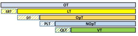
Figure 2.1: Production times and time losses classification starting out from an observation period OT (Zammori et al.,, 2011)

The Overall Equipment Effectiveness (OEE) is a widely-used index that weighs the actual capacity of equipment in relation to its optimal capacity and is defined as the product of the availability, performance and quality rates:

$$\texttt{oee}=\texttt{av}\times\texttt{pf}\times\texttt{qu}$$ [2.3]

The OEE is designed to trace the losses that are directly dependent on the equipment being used, while leaving out other losses that cannot be fixed by rearranging or repairing the equipment. Equivalently, the OEE can also be defined as

$$\texttt{oee}=\dfrac{\texttt{LT}-\texttt{DT}-\texttt{PLT}-\texttt{QLT}}{\texttt{LT}}=\dfrac{\texttt{VT}}{\texttt{LT}}$$

or

$$\texttt{oee}=\dfrac{\texttt{TU}-\texttt{DU}}{\texttt{ICS}\times\texttt{LT}},$$

where ICS is the ideal cycle speed (in cycles per time unit; a cycle, or unit, is a produced item), TU is the total number of units and DU the number of defective units. The last definition demonstrates that a $100\%$ value in the OEE is obtained under optimal working conditions, that is, when the process has produced only flawless items at the ideal speed during the scheduled working hours. In Zammori et al., (2011) the OEE was considered a random variable and its distribution was used to assess the effectiveness of correction actions implemented in the maintenance strategy. Different time losses are deemed as independent beta random variables, but the independency assumption might be taken as unrealistic in real-life processes where, for example, a major failure is often preceded -or followed- by slower production speeds or by a higher number of rejected units. In our work, we will also investigate whether the dependency between losses leads to a better predictive model.

3 The model

3.1 Input-Ouput Hidden Markov Model

We model the production process as an IO-HMM, i.e., an HMM with an input stream. Figure 3.1 depicts the diagram of an IO-HMM. The main assumption in HMMs is that the process goes through $K$ hidden states according to an initial state probability distribution and a transition probability distribution between states. The hidden state of the $n$-th observation period is denoted by $c_{n}$ and ideally stands for the condition or the operational mode of the production process during that period. Each state gives rise to a different probability distribution of the continuous responses in the output stream, that are denoted by $\mathbf{y}_{n}$. The decision about the number of hidden states will be discussed in Section 4.3.

The distinctive feature of an IO-HMM is that the model’s probability distributions are affected by an input stream of covariates, denoted by $\mathbf{x}_{n}$. These covariates, which may include among others calendar variables or the reference produced, characterize the observation period that is about to begin. Further, we introduce an autoregressive component into the model by allowing the covariates to include past values of the response variables. The covariates that influence the probabilities in the discrete part of the model will be denoted by $\mathbf{z}_{n}\subseteq\mathbf{x}_{n}$, while those that impact the responses’ joint density will be denoted by $\mathbf{w}_{n}\subseteq\mathbf{x}_{n}$. Both discrete and continuous processes of the model are thoroughly described in the upcoming sections.

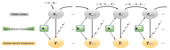
Figure 3.1: Diagram of an IO-HMM. Covariates $\mathbf{x}_{n}$ affect both discrete and continuous processes. Probabilities in the discrete process $\left\{c_{n}\right\}_{n\geq 1}$ are dependent on covariates $\mathbf{z}_{n}\subseteq\mathbf{x}_{n}$ and probabilities in the continuous process $\left\{\mathbf{y}_{n}\right\}_{n\geq 1}$ are dependent on covariates $\mathbf{w}_{n}\subseteq\mathbf{x}_{n}$.

3.2 The discrete process

Assume that the discrete process $\{c_{n}\}_{n\geq 1}$ is a Markov chain with $K$ different states, that is, $c_{n}\in\left\{1,\ldots,K\right\},\ n\geq 1$. The probability distributions for the initial state and the transitions between states are dependent on the covariates $\mathbf{z}_{n}$, that are assumed to take values in a discrete and finite set of $S$ symbols, i.e., $\mathbf{z}_{n}\in\left\{1,\ldots,S\right\},\ n\geq 1$.

For a given $s\in\left\{1,\ldots,S\right\}$, we assume that the initial probabilities $\bm{\pi}^{(s)}=\mathbb{P}\left[c_{1}|\mathbf{z}_{1}=s\right]$ and the transition probabilities $\mathbf{p}_{k}^{(s)}=\mathbb{P}\left[c_{n}|c_{n-1}=k,\mathbf{z}_{n}=s\right],\ k=1,\ldots,K$ follow Dirichlet prior distributions, that is,

$$\bm{\pi}^{(s)}=\left[\pi_{1}^{(s)}\ldots\ \pi_{K}^{(s)}\right] \sim\textrm{Dirichlet}\left(\mathbf{a}^{(s)}=[a^{(s)}_{1}\ \ldots\ a^{(s)}_{K}]\right)$$

$$\mathbf{p}_{k}^{(s)}=\left[p_{k1}^{(s)}\ \ldots\ p_{kK}^{(s)}\right] \sim\textrm{Dirichlet}\left(\bm{\alpha}^{(s)}_{k}=[\alpha^{(s)}_{k1}\ \ldots\ \alpha^{(s)}_{kK}]\right).$$ [3.1]

It is well-known that the parameters of a Dirichlet distribution can be recognized as pseudo-counts of the events represented by the random probabilities so that, for example, $\pi_{k}^{(s)}$ is the pseudo-count of sequences with covariate $\mathbf{z}_{1}=s$ starting in state $k$ and $\alpha_{kj}^{(s)}$ is the pseudo-count of transitions from state $k$ to state $j$ when the covariates have the value $s$. We will denote by

$$a_{0}^{(s)}\stackrel{{\scriptstyle def}}{{=}}\sum_{k=1}^{K}a_{k}^{(s)}\quad\text{ and }\quad\alpha_{k0}^{(s)}\stackrel{{\scriptstyle def}}{{=}}\sum_{j=1}^{K}\alpha_{kj}^{(s)}$$

the concentration parameters of each distribution.

Conditioned to the last observed state, the next unobserved state is a random variable following a categorical distribution (or multinomial with one single trial) with parameters $\bm{\pi}^{(s)}$ if the sequence just begins or with parameters $\mathbf{p}_{k}^{(s)}$ if the previous observation of the same sequence is in state $k$. Since a prior Dirichlet and a categorical likelihood are conjugate, the posterior distribution for the parameters is also Dirichlet with revised pseudo-counts. Thus, when a new output measurement become available it is assigned to the most probable state, say $j$, and the relevant pseudo-count is updated by increasing the parameter $a^{(s)}_{j}$ or $\alpha^{(s)}_{kj}$ by $1$.

3.3 The continuous process

The continuous process $\{\mathbf{y}_{n}\}_{n\geq 1}$ arises from a density function dependent on the state $c_{n}$ and the covariates $\mathbf{w}_{n}$. We develop a multivariate extension of the model presented in Alvarez et al., (2021) and split the conditional distribution of $\mathbf{y}_{n}|c_{n},\mathbf{w}_{n}$ into two independent conditional distributions

$$\mathbf{y}_{n}|\mathbf{w}_{n} \sim\mathcal{N}_{m}(\mathbf{u}_{n}\mathbf{H}_{u},\bm{\Sigma}_{u})$$ [3.2a]

$$\mathbf{y}_{n}|c_{n} \sim\mathcal{N}_{m}(\mathbf{v}_{n}\mathbf{H}_{v},\bm{\Sigma}_{v}),$$ [3.2b]

where $m$ is the number of response variables, $\mathbf{H}_{u},\mathbf{H}_{v}$ denote coefficient matrices, $\bm{\Sigma}_{u},\bm{\Sigma}_{v}$ are covariance matrices, $\mathbf{u}_{n}=\left[1\ \mathbf{w}_{n}^{T}\right]$ and $\mathbf{v}_{n}=v(c_{n})$, with $v(\cdot)$ a function of the hidden state. We propose considering the conditional expectation $v(c_{n})=\mathbb{E}\left[c_{n}|c_{n-1}\right]$, which, with the Dirichlet distribution assumptions, simplifies to the Dirichlet parameters in [3.1] normalized by their concentration parameters, i.e., $\mathbf{v}_{n}=\mathbf{a}/a_{0}$ or $\mathbf{v}_{n}=\bm{\alpha}_{c_{n-1}}/\alpha_{c_{n-1},0}$.

3.4 The adaptive algorithm

Let $\lambda\in(0,1]$ be a forgetting factor that accounts for the weight of past observations, and for the sake of clarity let us omit subscripts for now. As soon as a new sample $\mathbf{y}_{n}$ becomes available, the estimators $\left(\mathbf{H}_{n-1},\bm{\Sigma}_{n-1}\right)$ are updated to $\left(\mathbf{H}_{n},\bm{\Sigma}_{n}\right)$ through an adaptive algorithm described by the following equations:

$$\gamma_{n} =1+\lambda\gamma_{n-1}$$ [3.3a]

$$\mathbf{H}_{n} =\mathbf{H}_{n-1}+\frac{\mathbf{P}_{n-1}\mathbf{u}_{n}^{T}}{\lambda+\mathbf{u}_{n}\mathbf{P}_{n-1}\mathbf{u}_{n}^{T}}\left(\mathbf{y}_{n}-\mathbf{u}_{n}\mathbf{H}_{n-1}\right)$$ [3.3b]

$$\bm{\Sigma}_{n} =\bm{\Sigma}_{n-1}-\frac{1}{\gamma_{n}}\left[\bm{\Sigma}_{n-1}-\frac{\lambda\left(\mathbf{y}_{n}-\mathbf{u}_{n}\mathbf{H}_{n-1}\right)^{T}\left(\mathbf{y}_{n}-\mathbf{u}_{n}\mathbf{H}_{n-1}\right)}{\lambda+\mathbf{u}_{n}\mathbf{P}_{n-1}\mathbf{u}_{n}^{T}}\right]$$ [3.3c]

$$\mathbf{P}_{n} =\frac{1}{\lambda}\left(\mathbf{P}_{n-1}-\frac{\mathbf{P}_{n-1}\mathbf{u}_{n}^{T}\mathbf{u}_{n}\mathbf{P}_{n-1}}{\lambda+\mathbf{u}_{n}\mathbf{P}_{n-1}\mathbf{u}_{n}^{T}}\right)$$ [3.3d]

initialized with $\mathbf{H}_{0}=\bm{0},\ \bm{\Sigma}_{0}=\bm{0},\ \mathbf{P}_{0}=\mathbf{I}$ and $\gamma_{0}=0$, where $\bm{0}$ is a matrix or vector of zeros and $\mathbf{I}$ the identity matrix. $\mathbf{P}_{n}$ is known as the state matrix. These equations can be obtained by extending to the multivariate case the Maximum-Likelihood-based proof provided in Alvarez et al., (2021), Thm. 1. We refer to Appendix 7 for the derivation of equations [3.3a]-[3.3d] using an alternative Bayesian approach.

3.5 Forecasting

After the training step, each distribution [3.2a]-[3.2b] produces a forecast of the responses. These forecasts are then combined using a minimum-variance criterion to obtain the final prediction (Roccazzella et al.,, 2022). Once a new observation is available the update-prediction loop begins again. In particular, when the parameters are updated after the $n$-th observation is received we can write

$$\mathbf{y}_{n+1,u}=\mathbf{u}_{n+1}\mathbf{H}_{u}+\bm{\varepsilon}_{n+1},\qquad \bm{\varepsilon}_{n+1}\sim\mathcal{N}_{m}(\bm{0},\bm{\Sigma}_{u})$$

$$\mathbf{y}_{n+1,v}=\mathbf{v}_{n+1}\mathbf{H}_{v}+\bm{\nu}_{n+1},\qquad \bm{\nu}_{n+1}\sim\mathcal{N}_{m}(\bm{0},\bm{\Sigma}_{v}),$$

and define the weighted process

$$\mathbf{y}_{n+1}=\mathbf{y}_{n+1,u}\mathbf{D}+\mathbf{y}_{n+1,v}(\mathbf{I}-\mathbf{D})$$

with $\mathbf{D}=\textrm{diag}\left(\delta_{1},\ldots,\delta_{m}\right)$ a diagonal weight matrix to be determined. The mean and covariance of this process provide a multivariate forecast of the responses at time $(n+1)$ and an estimate of its accuracy, namely

$$\mathbb{E}_{n}\left[\mathbf{y}_{n+1}\right]\stackrel{{\scriptstyle def}}{{=}}\hat{\mathbf{y}}_{n+1} =\mathbf{u}_{n+1}\mathbf{H}_{u}\mathbf{D}+\mathbf{v}_{n+1}\mathbf{H}_{v}(\mathbf{I}-\mathbf{D})$$ [3.4a]

$$\mathbb{V}\mathrm{ar}_{n}\left[\mathbf{y}_{n+1}\right]\stackrel{{\scriptstyle def}}{{=}}\hat{\bm{\Sigma}}_{n+1} =\mathbf{D}\bm{\Sigma}_{u}\mathbf{D}+(\mathbf{I}-\mathbf{D})\bm{\Sigma}_{v}(\mathbf{I}-\mathbf{D}),$$ [3.4b]

where the subindex $n$ in the expectation and variance operators denotes that they are applied given all the information available at time $n$. We note that finding $\mathbf{D}$ amounts to obtain separately the optimal weight $\delta_{j}$ for each response, $j=1,\ldots,m$. According to Alvarez et al., (2021) this weight is given by

$$\delta_{j}=\dfrac{\sigma_{v,j}^{2}}{\sigma_{u,j}^{2}+\sigma_{v,j}^{2}},$$ [3.5]

where $\sigma_{u,j}^{2}$ $(\sigma_{v,j}^{2})$ is the $j$-th diagonal element of $\mathbf{\Sigma}_{u}$ $\left(\mathbf{\Sigma}_{v}\right)$.

4 Methodology

4.1 Data Segmentation

We assume that all the time variables presented in Figure 2.1 are random. This decision introduces an additional and unusual random component, as most industrial processes are typically observed either continuously or at fixed times, and the planned stop times are known beforehand, meaning that variables OT, SBT, and LT are often deterministic. However, due to internal protocols of the data supplier company, most of the measurement times in our dataset are determined by random events. This has compelled us to take the first option. Nevertheless, there is always a measurement taken at the end of each sequence, and to make use of this information we consider that the process starts over whenever a new sequence begins, and that the observations are taken at random times during the sequence duration.

4.2 Covariate selection

It is important to carefully select both responses and covariates keeping in mind the final goal of the method, which is to forecast time losses and efficiency indexes in the next period. In the case of high correlation between responses, a multivariate model would prove more effective than separate univariate models. The covariates $\mathbf{x}_{n}$ are expected to have some impact on the initial state and transition probabilities of the discrete part of the model and the responses’ joint density of the continuous part, although each part could be affected by different covariates. We will assume that the covariates of the discrete part, $\mathbf{z}_{n}$, are discrete and that the covariates in the continuous part, $\mathbf{w}_{n}$, comprise both discrete and continuous variables. In particular, lagged values of the responses can be included in $\mathbf{w}_{n}$. In addition, some quantitative variables need to be selected for the next classification step either using a dimensionality reduction method like Principal Component Analysis (PCA) or by simple choice. These variables, referred to as classification variables, will be denoted by $\mathbf{t}_{n}$.

4.3 Clustering

The observations of the training set are grouped into $K\geq 2$ classes using an unsupervised classification technique according to the variables collected in the vector $\mathbf{t}_{n}$. The final number of classes is set as the minimum number needed to achieve a threshold in the goodness-of-fit (i.e., the between-groups-sum-of-squares divided by the total-sum-of-squares). If we identify the classes with different colours, after the classification step each sequence in the training set ends up broken into several coloured segments as depicted in Figure 4.1. The classes will encode the hidden states in the HMM and will be used to learn the parameters of the discrete part of the model as described in Section 3.2. This process is initialized with uninformative Jeffrey’s priors for the Dirichlet distributions [3.1], that is, $a_{k}=\alpha_{jk}=1/2,\ \forall j,k$.

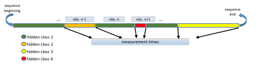
Figure 4.1: Sequence split into several intervals (OT) of different class

Let $\mathbf{o}_{k}$ be the centroid of the $k$-th class and $c_{n}$ the class of the $n$-th observation. Once the training step is complete, the observations in the test set are assigned to the closest centroid, that is

$$c_{n}=\operatorname*{arg\,min}_{k\in\{1,\ldots,K\}}d(\mathbf{o}_{k},\mathbf{t}_{n}),$$

where $d(a,b)$ is a distance function such as Euclidean or Mahalanobis. Another reasonable option is to classify the test observations via k-nearest-neighbors.

4.4 Implementation details

Let $\mathcal{S}$ be the set of symbols in $\mathbf{z}_{n}$ and $\mathcal{K}$ the set of hidden states. We define the sets of parameters

$$\bm{\Pi} =\left\{\mathbf{a}_{s}=[a^{(s)}_{1}\ \ldots\ a^{(s)}_{K}],\mathbf{A}_{s}=\left(\alpha_{kj}^{(s)}\right)_{k,j\in\mathcal{K}},s\in\mathcal{S}\right\}$$

$$\bm{\Psi} =\left\{\mathbf{H}_{u}^{(s)},\bm{\Sigma}_{u}^{(s)},\mathbf{H}_{v}^{(s)},\bm{\Sigma}_{v}^{(s)},\ s\in\mathcal{S}\right\}$$

$$\bm{\Omega} =\left\{\mathbf{P}_{u}^{(s)},\gamma_{u}^{(s)},\mathbf{P}_{v}^{(s)},\gamma_{v}^{(s)},\ s\in\mathcal{S}\right\}$$

where

• $a_{k}^{(s)}$ is the count of sequences starting in state $k$ with covariates of type $s$,

• $\alpha_{kj}^{(s)}$ is the count of transitions from state $k$ to state $j$ for observations with covariates of type $s$,

• $\mathbf{H}_{\;\bullet}^{(s)},\bm{\Sigma}_{\;\bullet}^{(s)}$ are coefficient and covariance matrices respectively,

• $\mathbf{P}_{\;\bullet}^{(s)},\gamma_{\;\bullet}^{(s)}$ are state matrices and discount factors respectively.

Pseudo-code for learning and forecasting methods is presented in Algorithms 1 and 2, whereas Figure 4.2 shows the block diagram of the adaptive algorithm for estimating the model parameters.

Input:

$\bm{\Pi}$	Dirichlet parameters
$\bm{\Psi}$	model parameters
$\bm{\Omega}$	state parameters
$\lambda_{u},\lambda_{v}$	forgetting factors
$\mathbf{x}_{n}=\left[\mathbf{z}_{n}\ \mathbf{w}_{n}\right]$	covariates
$c_{n-1},c_{n},\mathbf{y}_{n}$	state labels, responses

1

Output:

$\bm{\Pi},\ \bm{\Psi},\ \bm{\Omega}$

updated parameters

2 for $n=1,\ldots,N$ do

3      $s\leftarrow\mathbf{z}_{n}$

4      $k\leftarrow c_{n-1}$

5      $\mathbf{b}\leftarrow\begin{cases}\mathbf{a}^{(s)}&\text{if the sequence begins},\\ \bm{\alpha}^{(s)}_{k}&\text{otherwise}\end{cases}$

6      $\mathbf{u}\leftarrow\left[1\ \mathbf{w}_{n}\right]$

7      $\mathbf{v}\leftarrow\mathbf{b}/\left(\mathbf{b}\cdot\mathbf{1}\right)$

8      Update $\gamma_{u}^{(s)},\mathbf{H}_{u}^{(s)},\bm{\Sigma}_{u}^{(s)},\mathbf{P}_{u}^{(s)}$ using equations [3.3a], [3.3b], [3.3c], [3.3d] respectively

9      Update $\gamma_{v}^{(s)},\mathbf{H}_{v}^{(s)},\bm{\Sigma}_{v}^{(s)},\mathbf{P}_{v}^{(s)}$ using equations [3.3a], [3.3b], [3.3c], [3.3d] respectively

10      $j\leftarrow c_{n}$

11      if the sequence begins then

12          $a^{(s)}_{j}\leftarrow a^{(s)}_{j}+1$

13           else

14               $\alpha_{kj}^{(s)}\leftarrow\alpha_{kj}^{(s)}+1$

15               

16                end for

Algorithm 1 Learning

Input:

$\bm{\Psi}$	model parameters
$\left\{\mathbf{o}_{1},\ldots,\mathbf{o}_{K}\right\}$	class centroids
$\mathbf{t}_{n}$	classification variables
$\mathbf{x}_{n+1}=\left[\mathbf{z}_{n+1}\ \mathbf{w}_{n+1}\right]$	covariates

1

Output:

$\hat{\mathbf{y}}_{n+1},\ \hat{\bm{\Sigma}}_{n+1}$

responses forecast, prediction error

2

3$k\leftarrow\operatorname*{arg\,min}_{j\in\{1,\ldots,K\}}d(\mathbf{o}_{j},\mathbf{t}_{n})$

4 Update $\mathbf{o}_{k}$ including $\mathbf{t}_{n}$

5 $s\leftarrow\mathbf{z}_{n+1}$

6 $\mathbf{b}\leftarrow\begin{cases}\mathbf{a}^{(s)}&\text{if the sequence begins}\\ \bm{\alpha}^{(s)}_{k}&\text{otherwise}\end{cases}$

7 $\mathbf{u}\leftarrow\left[1\ \mathbf{w}_{n+1}\right]$

8 $\mathbf{v}\leftarrow\mathbf{b}/\left(\mathbf{b}\cdot\mathbf{1}\right)$

9 Compute $\mathbf{D}$ using equation [3.5]

10 Compute $\hat{\mathbf{y}}_{n+1}$ using equation [3.4a]

Compute $\hat{\bm{\Sigma}}_{n+1}$ using equation [3.4b]

Algorithm 2 Forecast

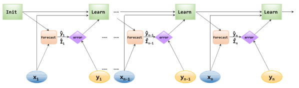
Figure 4.2: Block diagram of the adaptive algorithm for the parameter estimates. The error in the last prediction, $\mathbf{y}_{n-1}-\hat{\mathbf{y}}_{n-1}$, and the new covariates $\mathbf{x}_{n}$ feed the learning algorithm.

4.5 Evaluation

For the evaluation task, two standard forecasting metrics are computed - Mean Absolute Error (MAE) and Root Mean Squared Error (RMSE)- for each response variable. For a test set of L observations these metrics are defined as

$$\text{MAE}=\frac{1}{L}\sum\limits_{n=1}^{L}|y_{n}-\hat{y}_{n}|$$

$$\text{RMSE}=\sqrt{\frac{1}{L}\sum\limits_{n=1}^{L}\left(y_{n}-\hat{y}_{n}\right)^{2}}$$

We compare the performance of models with different numbers of response lags, $q=1,\ldots 5$, in the autoregressive component against the following benchmark models:

• The persistence model, which simply uses the last available observation to forecast the next one, that is $\hat{\mathbf{y}}_{n}=\mathbf{y}_{n-1}$.

• The no-lags model, which does not have an autoregressive component (i.e., $q=0$).

• The respective univariate models.

5 Application to a real case study

The proposed model has been employed to predict time losses in the production process of a company in a certain industrial sector. The specific industry of this company has been withheld due to confidentiality reasons. A digital platform is integrated along the manufacturing line to capture and store the production data stream. The data are supplied by the technological firm responsible for installing and maintaining the digital platform in the plant. To properly feed the presented method the data has been preprocessed, debugged and arranged using Python language (Van Rossum and Drake,, 1995) with some well-known libraries such as pandas (McKinney,, 2010) and numpy (Harris et al.,, 2020). The main core of the procedure, as described in Section 4, has been implemented in R language (R Core Team,, 2022).

After pruning and preprocessing the original data set, including the removal of periods without activity (weekends and holidays), the final data set comprises 7693 observations and 33 variables spanning 66 weeks of process activity. Table 5.1 shows a transcription of two entries of process data which consists of the following variables: observation id (n), date and starting hour of the observation (date, hour), working shift (shift), production order id (pr.ord), ideal unit speed (ics), number of total and defective units (TU, DU), target units under optimal conditions ($\texttt{TgU}=\texttt{OpT}\times\texttt{ics}$), opening time and stand-by time (OT, SBT), loading time (LT), real cycle speed ($\texttt{rcs}=\texttt{TU}/\texttt{LT}$), loading rate (lo), down time (DT), operating time (OpT), availability rate (av), performance time losses (PLT ), net operating time (NOpT), performance rate (pf), time losses due to quality issues (QLT), valuable time (VT), quality rate (qu), oee index, total number of stops (nstops) and average humidity and temperature (hum, temp. The time variables are measured in minutes.

Table 5.1: An example of production data after arrangement. In the shift column the first two letters indicate the weekday and the last one indicates the shift (Morning, Afternoon, Night).

n	date	start	shift	pr.ord	ics	TU	DU	TgU	OT	SBT	LT	rcs	lo
66	2022-10-10	13:50:24	Mo M	305	1.88	13	1	13.1	9.6	0	9.6	1.35	1
67	2022-10-10	14:00:00	Mo A	305	1.88	13	0	13.4	9.69	0	9.69	1.34	1
n	DT	OpT	av	PLT	NOpT	pf	QLT	VT	qu	oee	nstops	hum	temp
66	2.62	6.98	0.73	0.05	6.93	0.99	0.53	6.4	0.92	0.67	2	64.0	24.3
67	2.52	7.17	0.74	0.37	6.8	0.95	0	6.8	1	0.7	2	64.3	24.3

The time variables OpT, NOpT and VT are selected as responses. The sample correlation between these variables is very high (cor(OpT,NOpT)=0.86, cor(OpT,VT)=0.86, cor(VT,NOpT)=0.99) so a multivariate model is fully justified. According to the scheme presented in Figure 2.1 and the definitions [2], [2] and [2.3], predicting these variables enables the computation of important efficiency indexes and time losses. In fact, in the usual case of equispaced time measurements and scheduled stops known in advance (i.e., deterministic OT, SBT and LT) it is possible to compute all of the time losses and indexes. The only covariate $\mathbf{z}_{n}$ that affects the probability distributions of the discrete model is shift, while the covariates $\mathbf{w}_{n}$ considered for the continuous part are shift, ics and two indicator variables identifying the first observation of each shift and the first observation of each production order. Further, an autoregressive component is considered by including past values of the responses as covariates. The classification step is performed using the variables considered most related to the process health, lo, av, pf, qu, oee, OT, rcs and TU, as the classification criteria. These variables are collected in the vector $\mathbf{t}_{n}$.

Over a grid of values in the interval $[0.9,1]$, forgetting factors $\lambda_{u}=0.99,\ \lambda_{v}=0.95$ are taken by inspection. Additional trials have shown that values below $0.9$ provide lower performance. Then, six models with $q$ responses lags, $q=0,1,2,3,4,5$, are implemented and trained using the last ten shifts of each type. For the forecasting step, two shifts of each type are predicted and the performance metrics MAE and RMSE are computed separately for each type of shift $s\in\mathcal{S}$.

Figure 5.1 provides an insight about the distribution of the metrics across shifts for each output variable. The box-plot layouts suggest that for every metric and every response (i) taking lags improves the average prediction performance with respect to the naive persistence model and with respect to the no-lags model: boxes on the top -persistence model- and on the bottom -no lags model- of each panel systematically have larger Q1, Q2 and Q3 values than middle boxes, and (ii) the model appears to be quite insensitive to the number of lags, given the similarity between the five boxes in the middle of each panel. The magnitudes of the average metrics are reasonable considering the responses sample quantiles and mean in the test set shown in Table 5.2. On the other hand, Figure 5.2 suggest that a multivariate model has a better prediction performance and, as expected, smaller prediction error than the univariate models.

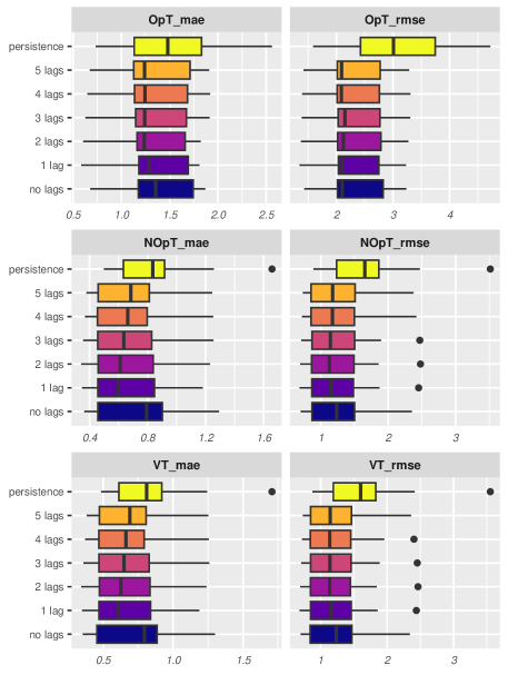
Figure 5.1: Boxplot of average metrics (by columns) across shifts for each output variable (by rows). Upper (persistence model) and lower (no-lags model) boxes show higher Q1, Q2 and Q3 values than models with autoregressive component, although the lag order seems to play a minor role.

Table 5.2: Responses sample mean and quantiles in the test set.

	min	Q1	median	mean	Q3	max
OpT	0	7.73	9.53	9.36	10.98	19.27
NOpT	0	4.67	5.42	6.32	7.0	16.8
VT	0	4.67	5.35	6.27	7.0	16.8

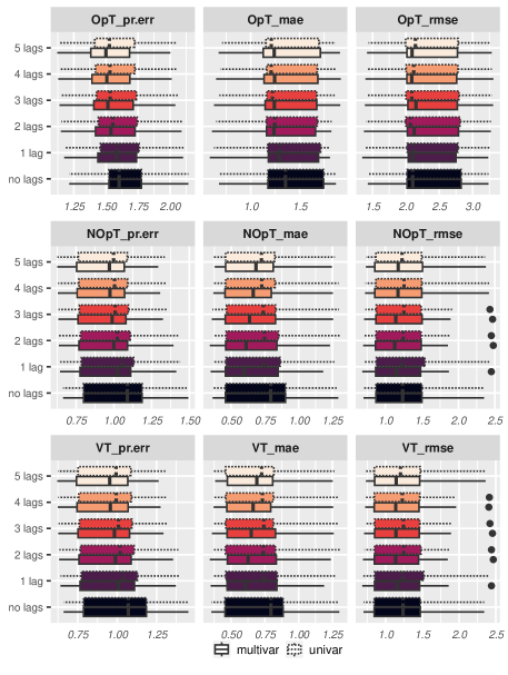
Figure 5.2: Comparison between multivariate and univariate models. In all but a few cases the multivariate model outperforms the univariate version on both metrics and presents tighter prediction error

6 Conclusions

In this work, we propose a probabilistic alternative for modelling industrial operational stream data based on an IO-HMM multivariate framework that incorporates an adaptive learning algorithm to ensure that the parameter estimates are updated using the most recent data. The model is designed to obtain probabilistic predictions of time variables, from which other relevant process quantities such as performance indexes can be deduced. In addition, the recursive nature of the estimation algorithm and the efficient implementation of the learning and forecasting stages substantially reduce the computational load of the method. This point makes it particularly suitable to be implemented in real-time applications. We compare the prediction performance of the proposed model with some benchmark models in a challenging data set that comes from a real production process that exhibits high variability, a recurrent affection in real-life industrial processes. Even then, the experimental results show that the predictions made by the proposed model are consistently more accurate than those of the standard baseline models.

Data availability statement

The data that support the findings of this study are available from the corresponding author upon reasonable request. The code to reproduce results with anonymized data will be available at:

https://github.com/spatialstatisticsupna/.

Disclosure statement

No potential conflict of interest was reported by the author(s).

7 Appendix

Proof of equations [3.3a]-[3.3d]

• Following the directions of Rossi et al., (2005), pp. 31–34, suppose a $m$-multivariate regression model with $p$ predictor variables

  $$\begin{cases}Y_{1}=&X\beta_{1}+\varepsilon_{1}\\ Y_{2}=&X\beta_{2}+\varepsilon_{2}\\ &\cdots\\ Y_{m}=&X\beta_{m}+\varepsilon_{m}\end{cases}$$

  with errors correlated across equations. For the $n$-th observation in a random sample of size $N$,

  $$\begin{bmatrix}y_{n1}\\ \vdots\\ y_{nm}\end{bmatrix} =\begin{bmatrix}\beta_{1}^{T}\\ \vdots\\ \beta_{m}^{T}\end{bmatrix}\begin{bmatrix}x_{n1}\\ \vdots\\ x_{np}\end{bmatrix}+\begin{bmatrix}\varepsilon_{n1}\\ \vdots\\ \varepsilon_{nm}\end{bmatrix}$$

  $$\underset{\underset{m\times 1}{\uparrow}}{Y_{n}} =\underset{\underset{m\times p}{\uparrow}}{B^{T}}\underset{\underset{p\times 1}{\uparrow}}{X_{n}}+\underset{\underset{m\times 1}{\uparrow}}{\bm{\varepsilon}_{n}}\qquad\text{ with }\qquad\bm{\varepsilon}_{n}\stackrel{{\scriptstyle iid}}{{\sim}}\mathcal{N}_{m}(\bm{0},\Lambda),\ n=1,2,\ldots,N$$

  and gathering all

  $$\begin{bmatrix}Y_{1}^{T}\\ \vdots\\ Y_{N}^{T}\end{bmatrix} =\begin{bmatrix}x_{11}&\cdots&x_{1p}\\ \vdots&\cdots&\vdots\\ x_{N1}&\cdots&x_{Np}\end{bmatrix}\begin{bmatrix}\beta_{1}&\cdots&\beta_{m}\end{bmatrix}+\begin{bmatrix}\bm{\varepsilon}_{1}^{T}\\ \vdots\\ \bm{\varepsilon}_{N}^{T}\end{bmatrix}$$

  $$\underset{\underset{N\times m}{\uparrow}}{Y} =\underset{\underset{N\times p}{\uparrow}}{X}\underset{\underset{p\times m}{\uparrow}}{B}+\underset{\underset{N\times m}{\uparrow}}{E}$$

  For some $\Lambda_{0}\in\mathcal{M}_{m\times m},\ N_{0}\in\mathbb{N},\ \beta_{0}\in\mathcal{M}_{mp\times 1},\ V_{0}\in\mathcal{M}_{p\times p}$, the natural conjugate priors for the parameters in the multivariate regression model can be taken as

  $$\mathbb{P}\left[\Lambda,B\right] =\mathbb{P}\left[B|\Lambda\right]\mathbb{P}\left[\Lambda\right]$$

  $$\Lambda \sim\mathcal{W}^{-1}(N_{0}\Lambda_{0},m,N_{0}+m+1)$$

  $$\beta|\Lambda \sim\mathcal{N}_{mp}\left(\beta_{0},\Lambda\otimes V_{0}^{-1}\right)$$

  where $\mathcal{W}^{-1}$ denotes a inverted Wishart distribution, $\otimes$ is the Kronecker product and $\beta=\textrm{vec}\left(B\right)$ (vectorization). The prior means are $\mathbb{E}\left[B|\Lambda\right]=B_{0}$ and $\mathbb{E}\left[\Lambda\right]=\Lambda_{0}$.

  Given these priors and the random sample, it is well known that the posterior joint density for the parameters can be decomposed into the product of the following densities

  $$\Lambda|Y,X \sim\mathcal{W}^{-1}\left(N_{0}\Lambda_{0}+N\tilde{S},m,N_{0}+N+m+1\right)$$

  $$\beta|\Lambda,Y,X \sim\mathcal{N}_{mp}\left(\tilde{\beta},\Lambda\otimes\left(X^{T}X+V_{0}\right)^{-1}\right)$$

  where

  $$\tilde{\beta} =\textrm{vec}\left(\tilde{B}\right)$$

  $$\tilde{B} =B_{0}+\left(X^{T}X+V_{0}\right)^{-1}X^{T}\left(Y-XB_{0}\right)$$

  $$N\tilde{S} =\left(Y-X\tilde{B}\right)^{T}\left(Y-X\tilde{B}\right)+\left(\tilde{B}-B_{0}\right)^{T}V_{0}\left(\tilde{B}-B_{0}\right).$$ [7.1a]

  Hence, the posterior means are

  $$\mathbb{E}\left[B|\Lambda\right] =\tilde{B}=B_{0}+\left(X^{T}X+V_{0}\right)^{-1}X^{T}\left(Y-XB_{0}\right)$$ [7.2a]

  $$\mathbb{E}\left[\Lambda|Y\right] =(N_{0}\underset{\underset{\text{prior mean}}{\uparrow}}{\Lambda_{0}}+N\tilde{S})/(N_{0}+N)$$

  $$=\Lambda_{0}-\dfrac{N\left(\Lambda_{0}-\tilde{S}\right)}{N_{0}+N}.$$ [7.2b]

• To make the above results fit in with our case let us define

  $$Y\ =\ \mathbf{y}_{n}\ \text{ (new responses, row vector $1\times m$)}$$

  $$X\ =\ \mathbf{u}_{n}\ \text{ (new predictors, row vector $1\times p$)}$$

  $$\tilde{B}\ =\ \mathbf{H}_{n}\ \text{ (posterior mean, $p\times m$)}$$

  $$B_{0}\ =\ \mathbf{H}_{n-1}\ \text{ (prior mean, $p\times m$)}$$

  $$V_{0}\ =\ \lambda\mathbf{P}_{n-1}^{-1}\ \text{ (prior state matrix, $p\times p$)}$$

  $$(X^{T}X+V_{0})^{-1}\ =\mathbf{P}_{n}\ \text{ (posterior state matrix, $p\times p$)}$$

  $$\gamma_{n}\ =1+\lambda+\cdots\lambda^{n-1}\ \text{(scalar)}$$

  Equation [3.3a] is obvious given that $\gamma_{n}=1+\lambda\left(1+\lambda+\cdots\lambda^{n-2}\right)=1+\lambda\gamma_{n-1}$. From the above definition of the posterior state matrix $\mathbf{P}_{n}$ and using the Sherman-Morrison formula,

  $$\mathbf{P}_{n} =\left(X^{T}X+V_{0}\right)^{-1}$$

  $$=\left(\mathbf{u}_{n}^{T}\mathbf{u}_{n}+\lambda\mathbf{P}_{n-1}^{-1}\right)^{-1}$$

  $$=\left(\lambda\mathbf{P}_{n-1}^{-1}\right)^{-1}-\dfrac{\left(\lambda\mathbf{P}_{n-1}^{-1}\right)^{-1}\mathbf{u}_{n}^{T}\mathbf{u}_{n}\left(\lambda\mathbf{P}_{n-1}^{-1}\right)^{-1}}{1+\mathbf{u}_{n}\left(\lambda\mathbf{P}_{n-1}^{-1}\right)^{-1}\mathbf{u}_{n}^{T}}$$

  $$=\dfrac{1}{\lambda}\left(\mathbf{P}_{n-1}-\dfrac{\mathbf{P}_{n-1}\mathbf{u}_{n}^{T}\mathbf{u}_{n}\mathbf{P}_{n-1}}{\lambda+\mathbf{u}_{n}\mathbf{P}_{n-1}\mathbf{u}_{n}^{T}}\right)$$

  we obtain equation [3.3d]. For the posterior mean $\tilde{B}=\mathbf{H}_{n}$, using expression [7.2a] we have

  $$\mathbf{H}_{n}=\tilde{B} =B_{0}+\left(X^{T}X+V_{0}\right)^{-1}X^{T}\left(Y-XB_{0}\right)$$

  $$=\mathbf{H}_{n-1}+\left(\mathbf{u}_{n}^{T}\mathbf{u}_{n}+\lambda\mathbf{P}_{n-1}^{-1}\right)^{-1}\mathbf{u}_{n}^{T}\left(\mathbf{y}_{n}-\mathbf{u}_{n}\mathbf{H}_{n-1}\right)$$

  $$=\mathbf{H}_{n-1}+\mathbf{P}_{n}\mathbf{u}_{n}^{T}\left(\mathbf{y}_{n}-\mathbf{u}_{n}\mathbf{H}_{n-1}\right)$$

  $$=\mathbf{H}_{n-1}+\dfrac{1}{\lambda}\left(\mathbf{P}_{n-1}-\dfrac{\mathbf{P}_{n-1}\mathbf{u}_{n}^{T}\mathbf{u}_{n}\mathbf{P}_{n-1}}{\lambda+\mathbf{u}_{n}\mathbf{P}_{n-1}\mathbf{u}_{n}^{T}}\right)\mathbf{u}_{n}^{T}\left(\mathbf{y}_{n}-\mathbf{u}_{n}\mathbf{H}_{n-1}\right)$$

  $$=\mathbf{H}_{n-1}+\dfrac{1}{\lambda}\dfrac{\mathbf{P}_{n-1}\mathbf{u}_{n}^{T}\left(\lambda+\mathbf{u}_{n}\mathbf{P}_{n-1}\mathbf{u}_{n}^{T}\right)-\mathbf{P}_{n-1}\mathbf{u}_{n}^{T}\mathbf{u}_{n}\mathbf{P}_{n-1}\mathbf{u}_{n}^{T}}{\lambda+\mathbf{u}_{n}\mathbf{P}_{n-1}\mathbf{u}_{n}^{T}}\left(\mathbf{y}_{n}-\mathbf{u}_{n}\mathbf{H}_{n-1}\right)$$

  $$=\mathbf{H}_{n-1}+\dfrac{\mathbf{P}_{n-1}\mathbf{u}_{n}^{T}}{\lambda+\mathbf{u}_{n}\mathbf{P}_{n-1}\mathbf{u}_{n}^{T}}\left(\mathbf{y}_{n}-\mathbf{u}_{n}\mathbf{H}_{n-1}\right),$$

  yielding equation [3.3b]. On the other hand, from the definition [7.1a] we get

  $$N\tilde{S} =\left(Y-X\tilde{B}\right)^{T}\left(Y-X\tilde{B}\right)+\left(\tilde{B}-B_{0}\right)^{T}V_{0}\left(\tilde{B}-B_{0}\right)$$

  $$=\left(\mathbf{y}_{n}-\mathbf{u}_{n}\mathbf{H}_{n}\right)^{T}\left(\mathbf{y}_{n}-\mathbf{u}_{n}\mathbf{H}_{n}\right)+\left(\mathbf{H}_{n}-\mathbf{H}_{n-1}\right)^{T}\left(\lambda\mathbf{P}_{n-1}^{-1}\right)\left(\mathbf{H}_{n}-\mathbf{H}_{n-1}\right)$$

  $$=\left[\mathbf{y}_{n}-\mathbf{u}_{n}\left(\mathbf{H}_{n-1}+\dfrac{\mathbf{P}_{n-1}\mathbf{u}_{n}^{T}}{\lambda+\mathbf{u}_{n}\mathbf{P}_{n-1}\mathbf{u}_{n}^{T}}\left(\mathbf{y}_{n}-\mathbf{u}_{n}\mathbf{H}_{n-1}\right)\right)\right]^{T}\left[\mathbf{y}_{n}-\mathbf{u}_{n}\left(\mathbf{H}_{n-1}+\dfrac{\mathbf{P}_{n-1}\mathbf{u}_{n}^{T}}{\lambda+\mathbf{u}_{n}\mathbf{P}_{n-1}\mathbf{u}_{n}^{T}}\left(\mathbf{y}_{n}-\mathbf{u}_{n}\mathbf{H}_{n-1}\right)\right)\right]+$$

  $$\phantom{=}\ \left[\dfrac{\mathbf{P}_{n-1}\mathbf{u}_{n}^{T}}{\lambda+\mathbf{u}_{n}\mathbf{P}_{n-1}\mathbf{u}_{n}^{T}}\left(\mathbf{y}_{n}-\mathbf{u}_{n}\mathbf{H}_{n-1}\right)\right]^{T}\left(\lambda\mathbf{P}_{n-1}^{-1}\right)\left[\dfrac{\mathbf{P}_{n-1}\mathbf{u}_{n}^{T}}{\lambda+\mathbf{u}_{n}\mathbf{P}_{n-1}\mathbf{u}_{n}^{T}}\left(\mathbf{y}_{n}-\mathbf{u}_{n}\mathbf{H}_{n-1}\right)\right]$$

  $$=\left[\left(\mathbf{y}_{n}-\mathbf{u}_{n}\mathbf{H}_{n-1}\right)-\dfrac{\mathbf{u}_{n}\mathbf{P}_{n-1}\mathbf{u}_{n}^{T}}{\lambda+\mathbf{u}_{n}\mathbf{P}_{n-1}\mathbf{u}_{n}^{T}}\left(\mathbf{y}_{n}-\mathbf{u}_{n}\mathbf{H}_{n-1}\right)\right]^{T}\left[\left(\mathbf{y}_{n}-\mathbf{u}_{n}\mathbf{H}_{n-1}\right)-\dfrac{\mathbf{u}_{n}\mathbf{P}_{n-1}\mathbf{u}_{n}^{T}}{\lambda+\mathbf{u}_{n}\mathbf{P}_{n-1}\mathbf{u}_{n}^{T}}\left(\mathbf{y}_{n}-\mathbf{u}_{n}\mathbf{H}_{n-1}\right)\right]+$$

  $$\phantom{=}\ \lambda\dfrac{\mathbf{u}_{n}\mathbf{P}_{n-1}\mathbf{u}_{n}^{T}}{\left(\lambda+\mathbf{u}_{n}\mathbf{P}_{n-1}\mathbf{u}_{n}^{T}\right)^{2}}\left(\mathbf{y}_{n}-\mathbf{u}_{n}\mathbf{H}_{n-1}\right)^{T}\left(\mathbf{y}_{n}-\mathbf{u}_{n}\mathbf{H}_{n-1}\right)$$

  $$=\left[\dfrac{\lambda\left(\mathbf{y}_{n}-\mathbf{u}_{n}\mathbf{H}_{n-1}\right)}{\lambda+\mathbf{u}_{n}\mathbf{P}_{n-1}\mathbf{u}_{n}^{T}}\right]^{T}\left[\dfrac{\lambda\left(\mathbf{y}_{n}-\mathbf{u}_{n}\mathbf{H}_{n-1}\right)}{\lambda+\mathbf{u}_{n}\mathbf{P}_{n-1}\mathbf{u}_{n}^{T}}\right]+\lambda\dfrac{\mathbf{u}_{n}\mathbf{P}_{n-1}\mathbf{u}_{n}^{T}}{\left(\lambda+\mathbf{u}_{n}\mathbf{P}_{n-1}\mathbf{u}_{n}^{T}\right)^{2}}\left(\mathbf{y}_{n}-\mathbf{u}_{n}\mathbf{H}_{n-1}\right)^{T}\left(\mathbf{y}_{n}-\mathbf{u}_{n}\mathbf{H}_{n-1}\right)$$

  $$=\dfrac{\lambda\left(\mathbf{y}_{n}-\mathbf{u}_{n}\mathbf{H}_{n-1}\right)^{T}\left(\mathbf{y}_{n}-\mathbf{u}_{n}\mathbf{H}_{n-1}\right)}{\lambda+\mathbf{u}_{n}\mathbf{P}_{n-1}\mathbf{u}_{n}^{T}}.$$

  Now, by choosing

  $$N_{0}\ =\ \lambda\gamma_{n-1}$$

  $$N\ =\ 1$$

  $$\Lambda_{0}\ =\bm{\Sigma}_{n-1}\ \text{ (prior mean variance, $m\times m$)}$$

  $$\mathbb{E}\left[\Lambda|Y\right]\ =\ \bm{\Sigma}_{n}\quad\text{ (posterior mean variance, $m\times m$)}$$

  and using expression [7.2b]

  $$\bm{\Sigma}_{n}=\mathbb{E}\left[\Lambda|Y\right]\ =\Lambda_{0}-\dfrac{N\left(\Lambda_{0}-\tilde{S}\right)}{N_{0}+N}$$

  $$=\bm{\Sigma}_{n-1}-\dfrac{1}{1+\lambda\gamma_{n-1}}\left[\bm{\Sigma}_{n-1}-\dfrac{\lambda\left(\mathbf{y}_{n}-\mathbf{u}_{n}\mathbf{H}_{n-1}\right)^{T}\left(\mathbf{y}_{n}-\mathbf{u}_{n}\mathbf{H}_{n-1}\right)}{\lambda+\mathbf{u}_{n}\mathbf{P}_{n-1}\mathbf{u}_{n}^{T}}\right]$$

  $$=\bm{\Sigma}_{n-1}-\dfrac{1}{\gamma_{n}}\left[\bm{\Sigma}_{n-1}-\dfrac{\lambda\left(\mathbf{y}_{n}-\mathbf{u}_{n}\mathbf{H}_{n-1}\right)^{T}\left(\mathbf{y}_{n}-\mathbf{u}_{n}\mathbf{H}_{n-1}\right)}{\lambda+\mathbf{u}_{n}\mathbf{P}_{n-1}\mathbf{u}_{n}^{T}}\right]$$

  follows equation [3.3c].

References

- Afzal and Al-Dabbagh, (2017) Afzal, M. S. and Al-Dabbagh, A. W. (2017). Forecasting in industrial process control: A Hidden Markov Model approach. IFAC-PapersOnLine, 50(1):14770–14775. 20th IFAC World Congress.
- Alvarez et al., (2021) Alvarez, V., Mazuelas, S., and Lozano, J. A. (2021). Probabilistic load forecasting based on adaptive online learning. IEEE Transactions on Power Systems, 36(4):3668––3680.
- Baruah and Chinnam, (2005) Baruah, P. and Chinnam, R. B. (2005). HMMs for diagnostics and prognostics in machining processes. International Journal of Production Research, 43(6):1275–1293.
- Bengio and Frasconi, (1996) Bengio, Y. and Frasconi, P. (1996). Input-output HMMs for sequence processing. IEEE transactions on Neural Networks, 7:1231–49.
- Chinnam and Baruah, (2009) Chinnam, R. B. and Baruah, P. (2009). Autonomous diagnostics and prognostics in machining processes through competitive learning-driven HMM-based clustering. International Journal of Production Research - INT J PROD RES, 47(23):6739–6758.
- Fischer et al., (2010) Fischer, A., Riesen, K., and Bunke, H. (2010). Graph similarity features for HMM-based handwriting recognition in historical documents. In 2010 12th International Conference on Frontiers in Handwriting Recognition, pages 253–258.
- Harris et al., (2020) Harris, C. R., Millman, K. J., van der Walt, S. J., Gommers, R., Virtanen, P., Cournapeau, D., Wieser, E., Taylor, J., Berg, S., Smith, N. J., Kern, R., Picus, M., Hoyer, S., van Kerkwijk, M. H., Brett, M., Haldane, A., Fernández del Río, J., Wiebe, M., Peterson, P., Gérard-Marchant, P., Sheppard, K., Reddy, T., Weckesser, W., Abbasi, H., Gohlke, C., and Oliphant, T. E. (2020). Array programming with NumPy. Nature, 585(7825):357–362.
- McKinney, (2010) McKinney, W. (2010). Data Structures for Statistical Computing in Python. In van der Walt, S. and Millman, J., editors, Proceedings of the 9th Python in Science Conference, pages 56–61.
- Muchiri and Pintelon, (2008) Muchiri, P. and Pintelon, L. (2008). Performance measurement using overall equipment effectiveness (OEE): Literature review and practical application discussion. International Journal of Production Research - INT J PROD RES, 46:3517–3535.
- R Core Team, (2022) R Core Team (2022). R: A Language and Environment for Statistical Computing. R Foundation for Statistical Computing, Vienna, Austria.
- Rabiner, (1989) Rabiner, L. (1989). A tutorial on hidden Markov models and selected applications in speech recognition. Proceedings of the IEEE, 77(2):257–286.
- Roblès et al., (2014) Roblès, B., Avila, M., Duculty, F., Vrignat, P., Bégot, S., and Kratz, F. (2014). Hidden Markov model framework for industrial maintenance activities. Proceedings of the Institution of Mechanical Engineers, Part O: Journal of Risk and Reliability, 228(3):230–242.
- Roccazzella et al., (2022) Roccazzella, F., Gambetti, P., and Vrins, F. (2022). Optimal and robust combination of forecasts via constrained optimization and shrinkage. International Journal of Forecasting, 38(1):97–116.
- Rossi et al., (2005) Rossi, P. E., Allenby, G. M., and McCulloch, R. (2005). Bayesian Statistics and Marketing. John Wiley and Sons, Ltd.
- Van Rossum and Drake, (1995) Van Rossum, G. and Drake, F. L. (1995). Python reference manual. Centrum voor Wiskunde en Informatica Amsterdam.
- Wójtowicz et al., (2019) Wójtowicz, D., Sason, I., Huang, X., Kim, Y.-A., Leiserson, M., Przytycka, T., and Sharan, R. (2019). Hidden Markov models lead to higher resolution maps of mutation signature activity in cancer. Genome Medicine, 11.
- Woodall and Montgomery, (2014) Woodall, W. H. and Montgomery, D. C. (2014). Some current directions in the theory and application of Statistical Process Monitoring. Journal of Quality Technology, 46(1):78–94.
- Yang and Zhong, (2022) Yang, R. and Zhong, M. (2022). Machine Learning-based fault diagnosis for industrial engineering systems. CRC Press.
- Zammori et al., (2011) Zammori, F., Braglia, M., and Frosolini, M. (2011). Stochastic overall equipment effectiveness. International Journal of Production Research, 49(21):6469–6490.