Consensus under Persistence Excitation
Abstract
We prove that a first-order cooperative system of interacting agents converges to consensus if the so-called Persistence Excitation condition holds. This condition requires that the interaction function between any pair of agents satisfies an integral lower bound. The interpretation is that the interaction needs to ensure a minimal amount of service.
I INTRODUCTION
Studying self-organization and emergence of patterns in collective dynamics has gained significant prominence in the control community. In particular, several researches have focused on understanding mechanisms underlying the dynamics of multi-agent systems, such as those enforcing the emergence of consensus. In simple terms, this means that all agents reach an agreement, as for instance a unanimous vote in elections. Applications of such models are found in a wide variety of fields, see e.g. [1, 2, 3, 4, 5, 6, 7].
In this article, we study first-order cooperative systems of the following form:
| (1) |
for where
for . It describes the evolution of agents on an Euclidean space . The position may represent opinion on different topics, velocity or other attributes of agent at time . The (nonlinear) influence function is used to quantify the influence of agent on agent , where . The term is a scaling parameter.
From the modelling point of view, each agent is expected to communicate with its neighbours through a network topology, influenced by sensor characteristics and the environment. While the easiest scenario involves a fixed network topology (e.g. [8, 9]), practical situations often involve dynamic changes, due to factors like communication dropouts, security concerns, or intermittent actuation. In this setting, potential connection losses between agents occur, hindering reaching consensus. Therefore, when interactions between agents are subject to failure, it becomes crucial to investigate whether consensus can still be achieved or not. We model this scenario as follows:
| (2) |
for . The terms represent the weight given to the (directed) connection of agent with agent . They encode the time-varying network topology and account for potential communication failures (e.g., when they vanish).
We quantify the possible lack of interactions by introducing the condition of persistent excitation (PE from now on).
Definition I.1 (Persistent excitation)
Let be given. We say that the function satisfies the PE condition with parameters if it holds
| (PE) |
Imposing the PE condition means that such a function is not too weak on any given time interval of length . This can be seen as a condition on the minimum level of service.
Although the PE condition is a standard tool in classical control theory (see [10, 11, 12]), its use in multi-agent systems has gained interest in the last years (see e.g. [13, 14, 15, 16]). Many of the results however impose a PE condition either on functions depending on the state of the system (see e.g. [15]), or on quantities like the averaged graph-Laplacian generated by the communication weights with respect to the variance bilinear form (see [16]) or the scrambling coefficients generated by the communication weights (see [17]). In all of these cases, the PE condition is then applied to quantities which in principle require a regular monitoring of the state of the system, instead of being applied to the communication weights only. In [18], for instance, the authors prove that consensus holds by applying the PE condition on symmetric communication weights only () which are moreover regulated in the sense that one-sided limits exist for all , and they consider only the case where .
The main result of this article shows that the PE condition on a general class of weights is sufficient to ensure consensus.
Theorem I.1
Let be a solution of (2) with initial data .
Assume the following conditions:
- (H1)
-
The function is Lipschitz continuous.
- (H2)
-
The constant
(3) satisfies .
- (H3)
-
All weights are -measurable.
Fix and assume that all satisfy (PE). Then, consensus holds:
The main interest of this result is given by the fact that consensus holds even under a very weak PE condition, e.g. when is very small and very large. This property is cleary connected with the fact that (2) is a cooperative system, i.e. interactions are always non-repulsive. Then, even when time runs with no interactions (or very weak ones), the overall configuration does not move far away from consensus.
We also show some simulations of systems of the form (2), see Section IV. While Theorem I.1 ensures convergence for any conditions, simulations allow to estimate the rate of convergence. Unsurprisingly, the average rate of convergence is decreasing as long as decreases. More surprisingly, the decrease is very regular (linear in log-log coordinates) , both for linear and non-linear dynamics.
The structure of the article is the following: in Section II, we describe two important models for opinion formation; we then provide some general properties of the dynamics. In Section III, we give the proof of the main result, first in the real line and then in the multidimensional setting. In Section IV, we show and discuss some simulations in the one-dimensional case. Finally, in Section V, we draw some conclusions and present future research directions.
II Models of opinion formation
In this section, we describe two important models for opinion formation of the form (1).
In the classical case, the function is symmetric and are fixed [19, 20]. In this setting, the average value is preserved and the system is cooperative. If the influence function satisfies condition ‣ INTRODUCTION, then all converge to the average value. However, such a setting has some scaling problems for large number of agents. Indeed, large groups of agents may have strong impact on small groups, even though they are very far from each other. For this reason, a different scaling has been proposed in [21]:
This rescaling introduces asymmetry in the dynamics, thus average is not preserved. Yet, also in this setting one reaches consensus under condition ‣ INTRODUCTION.
We treat both cases in a unitary way, from now on. For this reason, we define
| (4) | |||
| (5) | |||
| (6) | |||
| (7) |
We use the following inequalities later:
| (8) |
for all . They are direct consequences of the definitions above and the condition .
We also later use the following lemma, which proof is a direct computation.
The interest of this lemma is that it permits to reverse several results, e.g. properties about the maximum becoming properties about the minimum.
II-A General properties
In this section, we prove properties of solutions of (2). We first show that the diameter satisfies a dissipative property. Before doing so, we provide a useful lemma.
Lemma II.2
Let be a pair of indices such that
It then holds
Proof. The proof is entirely similar to the proof [17, Lemma 3.4] in the context of graphons.
Proposition II.1
The function
is non-increasing
Similarly, the size of the support
is non-increasing
Similarly, on the real line, the function
is non-decreasing.
Proof. The functions and are Lipschitz, since they are the pointwise maxima of a finite family of Lipschitz continuous functions. By Rademacher’s theorem, they are differentiable almost everywhere. By Dankin’s theorem (see [22]) it holds
where represents the nonempty subset of indices for which the maximum is reached. Fix an arbitrary and observe that for all it holds
which implies that for all it holds
Since this estimate holds for any , we have
i.e. the function is non-increasing.
The statement for the size of the support is recovered as follows. Again, by using Dankin’s theorem it holds
where represents the nonempty subset of pairs of indices for which the maximum is reached. Fix arbitrary . For easier notation, from now on we hide the dependence on time. Notice that for the case of normalized weights it holds
By Lemma II.2, for all it holds
and therefore, by (7), it holds
The statement for the minimum on the real line can be recovered by Lemma II.1.
II-B Dynamics on the real line
In this section, we study the case , i.e. in which the configuration space is the real line . In this setting, ordering is clearly a major advantage.
We introduce a useful operator, that is . The idea is that, given an initial configuration in which the position of all agents has a value larger than , the quantity represents a lower barrier for the position at time of a particle starting at .
Lemma II.3
Define
| (9) |
Let be a solution of (2) on that satisfies for all for some . If there exists an index and such that , then
| (10) |
Proof. Define and for compute
In the first term, we write
III Proof of Theorem I.1
In this section, we prove Theorem I.1. We first prove it for the 1-dimensional case, then for a general dimension .
III-A Proof in
In this section, we prove Theorem I.1 when the configuration space is .
Define the sequence . Since the sequence
| (11) |
is bounded, due to Proposition II.1, there exists as subsequence of , that we do not relabel, such that (11) is converging to some . Since the number of permutations of agents is finite, there exists a subsequence of , that we do not relabel, for which the order of particles is preserved. With no loss of generality, for a single relabeling, we assume
| (12) |
for all . This implies
| (13) |
We now prove that it holds . By contradiction, from now on we assume
| (14) |
We observe that for all it holds in the case of fixed weights and in the case of rescaled weights. It then holds
| (15) |
where is defined by (7). We now choose
| (16) |
Observe that and ensure
| (17) |
We recall that and . We then choose such that it holds and .
Claim 1. It holds . Similarly, it holds .
We prove the claim, by contradiction. If , i.e. for some , then for all due to (12). This implies hence . By Proposition II.1, this in turn implies for all . In particular, it holds . Thus, it holds . This contradicts the condition .
The condition can be easily recovered, by using Proposition II.1, and we have thus proved Claim 1.
We consider the trajectory of any agent with . We have two cases:
Recall that is given by (9) and is given by (18). We define , and for compute
where in the last inequality we have used (17). By using (15), we finally find
By integration in and using (PE), it holds
By merging the two cases, we proved that for all . By Proposition II.1, this implies that for all . In particular, this implies , hence . This is a contradiction.
Then, condition (14) is false and it holds . We now prove that this implies consensus. Indeed, for each choose such that . Observe that, due to Proposition II.1, for each it holds
and similarly . This implies
Since are arbitrary, it also holds . Then . Again by arbitrariness of indexes, the result is proved.
III-B Proof for any dimension
In this section, we prove Theorem I.1 on for any . The idea is to show that the dynamics can be projected on a line, and to use the result of Section III-A on such line.
The key observation is the following. Fix two vectors and take a solution of (2) in . Define the projected solution as
In general, it is clear that is not a solution of (2), since it holds
Yet, a careful look to the proof in Section III-A shows that the key properties ensuring the result are Proposition II.1 and estimates for the interaction kernels encoded in (8). In higher dimension, the fact that Proposition II.1 holds also implies that computed for the variables provide corresponding bounds for the interaction of the . As a consequence, Theorem I.1 also holds for the variables , for any choice of fixed .
We now prove the theorem. Consider the sequence of times . By Proposition II.1, the sequence is bounded. By passing to a subsequence , that we do not relabel, we have that the sequence is converging to some . Choose one among the maximizers of . With no loss of generality, we assume that it is realized by . Choose and . It is crucial to observe that they are fixed vectors. Define the variables and apply Theorem I.1 on the real line. It then holds for some common . By choosing , it holds , hence . By choosing , it holds
This implies , i.e. . By recalling that were chosen as maximizers of , this implies for all , i.e. . We rewrite it as follows: for all , there exists such that for all . By Proposition II.1 and recalling that is convex, we have that for all it holds . This is equivalent to for all , that implies consensus.
IV Simulations
In this section, we provide some simulations for the dynamics given by (2). For simplicity, we always study the dynamics of agents, with fixed and in the PE condition.
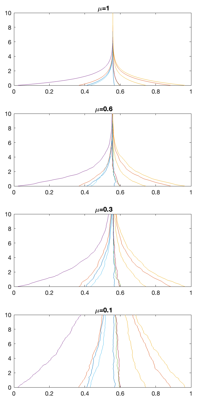
We first consider agents with initial positions randomly chosen from the uniform probability distribution on . For a given initial position, we show in Figure 1 four solutions of (2) with satisfying the PE condition with , respectively. It is clear that convergence always holds, in accordance with Theorem I.1. Yet, the rate of convergence decreases with the decrease of .
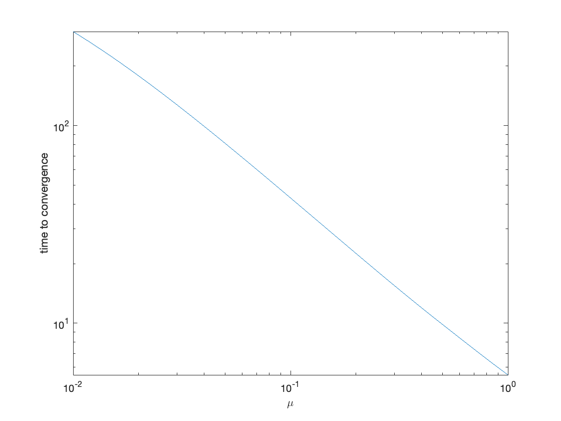
We investigate more in detail the rate of convergence as a function of . We consider different initial configurations and, for each of them and each value of , we compute the time to reach a diameter of . For each , we then consider the average of such times, that can be seen as a good measure of the rate of convergence. The result is provided in Figure 2, that is a log-log graph of the value of and the corresponding average time to convergence. The fact that the graph is linear shows that the average behavior is very regular: the PE condition becomes a uniform reduction of the interaction to . We aim to deepen the comprehension of this phenomenon in a future work.
V Conclusions and future directions
In this article, we have proved that the condition of Persistence Excitation (PE) is sufficient to ensure consensus of a cooperative multi-agent system.
The natural extension of this result would be to prove a similar result for second-order systems, such as those describing velocity alignement and flocking [23]. Yet, the natural difficulty in this project is the fact that our proof here does not provide a rate of convergence towards the consensus. In second-order systems, this corresponds to a lack of knowledge of the expansion of the support, undermining the certainty of having an interaction function bounded from below by a strictly positive constant, i.e. (H2).
Our project is then to provide quantitative estimates for the rate of convergence, as a first tool towards a more general applicability of the theory. The simulations provided here are a first step towards this direction.
References
- [1] C. Tomlin, G. J. Pappas, and S. Sastry, “Conflict resolution for air traffic management: A study in multiagent hybrid systems,” IEEE Trans. on auto. control, vol. 43, no. 4, pp. 509–521, 1998.
- [2] A. Jadbabaie, J. Lin, and A. S. Morse, “Coordination of groups of mobile autonomous agents using nearest neighbor rules,” IEEE Trans. on auto. control, vol. 48, no. 6, pp. 988–1001, 2003.
- [3] A. Benatti et al., “Opinion diversity and social bubbles in adaptive sznajd networks,” Journal of Stat. Mech.: Theory and Experiment, vol. 2020, no. 2, p. 023407, 2020.
- [4] S. M. Krause and S. Bornholdt, “Opinion formation model for markets with a social temperature and fear,” Physical Review E, vol. 86, no. 5, p. 056106, 2012.
- [5] Q. Zha et al., “Opinion dynamics in finance and business: a literature review and research opportunities,” Fin. Innov., vol. 6, pp. 1–22, 2020.
- [6] Y.-l. Chuang et al., “State transitions and the continuum limit for a 2d interacting, self-propelled particle system,” Physica D: Nonlinear Phen., vol. 232, no. 1, pp. 33–47, 2007.
- [7] N. Bellomo, M. A. Herrero, and A. Tosin, “On the dynamics of social conflicts: Looking for the black swan,” Kinetic and Related Models, vol. 6, no. 3, pp. 459–479, 2013.
- [8] D. J. Watts and S. H. Strogatz, “Collective dynamics of ‘small-world’networks,” Nature, vol. 393, no. 6684, pp. 440–442, 1998.
- [9] R. Olfati-Saber, J. A. Fax, and R. M. Murray, “Consensus and cooperation in networked multi-agent systems,” Proceedings of the IEEE, vol. 95, no. 1, pp. 215–233, 2007.
- [10] K. S. Narendra and A. M. Annaswamy, Stable adaptive systems. Courier Corporation, 2012.
- [11] Y. Chitour and M. Sigalotti, “On the stabilization of persistently excited linear systems,” SIAM Journal on Control and Optimization, vol. 48, no. 6, pp. 4032–4055, 2010.
- [12] Y. Chitour, F. Colonius, and M. Sigalotti, “Growth rates for persistently excited linear systems,” Mathematics of Control, Signals, and Systems, vol. 26, no. 4, pp. 589–616, 2014.
- [13] W. Ren and R. W. Beard, Distributed consensus in multi-vehicle cooperative control, vol. 27. Springer, 2008.
- [14] Z. Tang, R. Cunha, T. Hamel, and C. Silvestre, “Bearing leader-follower formation control under persistence of excitation,” IFAC-PapersOnLine, vol. 53, no. 2, pp. 5671–5676, 2020.
- [15] S. Manfredi and D. Angeli, “A criterion for exponential consensus of time-varying non-monotone nonlinear networks,” IEEE Trans. on Auto. Control, vol. 62, no. 5, pp. 2483–2489, 2016.
- [16] B. Bonnet and E. Flayac, “Consensus and flocking under communication failures for a class of cucker–smale systems,” Systems & Control Letters, vol. 152, p. 104930, 2021.
- [17] B. Bonnet, N. Pouradier Duteil, and M. Sigalotti, “Consensus formation in first-order graphon models with time-varying topologies,” Mathematical Models and Methods in Applied Sciences, vol. 32, no. 11, pp. 2121–2188, 2022.
- [18] B. D. Anderson, G. Shi, and J. Trumpf, “Convergence and state reconstruction of time-varying multi-agent systems from complete observability theory,” IEEE Transactions on Automatic Control, vol. 62, no. 5, pp. 2519–2523, 2016.
- [19] R. Hegselmann and U. Krause, “Opinion dynamics and bounded confidence: models, analysis and simulation,” Journal of Artificial Societies and Social Simulation, vol. 5, no. 3, p. 2, 2002.
- [20] M. H. DeGroot, “Reaching a consensus,” Journal of the American Statistical association, vol. 69, no. 345, pp. 118–121, 1974.
- [21] S. Motsch and E. Tadmor, “A new model for self-organized dynamics and its flocking behavior,” J. Stat. Phys., vol. 144, pp. 923–947, 2011.
- [22] J. M. Danskin, The theory of max-min and its application to weapons allocation problems, vol. 5. Springer Science & Business Media, 2012.
- [23] F. Cucker and S. Smale, “On the mathematical foundations of learning,” Bull. AMS, vol. 39, no. 1, pp. 1–49, 2002.