Turbulent mixed convection in vertical and horizontal channels
Abstract
Turbulent shear flows driven by a combination of a pressure gradient and buoyancy forcing are investigated using direct numerical simulations. Specifically, we consider the setup of a differentially heated vertical channel subject to a Poiseuille-like horizontal pressure gradient. We explore the response of the system to its three control parameters: the Grashof number Gr, the Prandtl number , and the Reynolds number of the pressure-driven flow. From these input parameters, the relative strength of buoyancy driving to the pressure gradient can be quantified by the Richardson number . We compare the response of the mixed vertical convection configuration to that of mixed Rayleigh–Bénard convection and find a nearly identical behaviour, including an increase in wall friction at higher Gr and a drop in the heat flux relative to natural convection for . This closely matched response is despite vastly different flow structures in the systems. No large-scale organisation is visible in visualisations of mixed vertical convection – an observation that is quantitatively confirmed by spectral analysis. This analysis, combined with a statistical description of the wall heat flux, highlights how moderate shear suppresses the growth of small-scale plumes and reduces the likelihood of extreme events in the local wall heat flux. Vice versa, starting from a pure shear flow, the addition of thermal driving enhances the drag due to the emission of thermal plumes.
keywords:
turbulent convection, turbulent boundary layers, buoyant boundary layers1 Introduction
The transport of heat by turbulent convection is integral to a wide range of natural and engineering applications, from building ventilation to the atmospheric boundary layer and the near-surface ocean. All of these examples can, under the right conditions, be classified as mixed convection. Mixed convection describes the scenario where both buoyancy and shear forces are relevant to the dynamics. This is in contrast to natural convection, where a flow is solely driven by density differences within the fluid, and forced convection, where buoyancy is negligible and the transport of heat is identical to that of a passive scalar. The relative importance of buoyancy compared to the imposed shear is quantified by the Richardson number , with the extreme cases for purely thermal driving and for purely shear or pressure driving.
The foundational work on mixed convection by Obukhov (1946) was motivated by understanding the dynamics of the surface layer of the atmosphere. Obukhov supposed that the dynamics were solely determined by the surface friction (quantified by the friction velocity ), the surface heat flux , and gravity , such that dimensional analysis revealed a single possible length scale that could describe the system. Using this length to rescale the problem, Monin & Obukhov (1954) derived what is now known as the Monin–Obukhov Similarity Theory (MOST) where ‘universal’ functions of are used to describe the mean velocity and temperature profiles in stably or unstably stratified shear flows. These universal functions are obtained by interpolating between the extreme cases of natural convection and forced convection, which were updated by Kader & Yaglom (1990) for unstable (i.e. convecting) boundary layers. A historical overview of MOST is provided in Foken (2006) and the theory has been extremely popular in atmospheric and oceanic applications. However, some of the assumptions underlying MOST have recently been coming under further scrutiny, particularly the power-law dependence of the mean profiles in the convective regime (Cheng et al., 2021).
Mixed convection has also often been studied in simple, canonical flow configurations where the system response is only dependent on a small number of dimensionless input parameters. A popular approach has been to introduce shear forcing into the classical Rayleigh–Bénard setup, either through a horizontal pressure gradient (Poiseuille–Rayleigh–Bénard, P-RB) or by setting one of the boundary plates in motion (Couette–Rayleigh–Bénard, C-RB). The linear stability of the P-RB system was studied by Gage & Reid (1968) who found that streamwise perturbations are suppressed by the introduction of shear, so the fastest growing mode takes the form of convective rolls in the plane orthogonal to the mean flow. Note that the critical Rayleigh number and the fastest growing wavelength do not change compared to natural RB since the linear problem is unchanged in the orthogonal plane. Such streamwise-aligned rolls were observed experimentally by Richter & Parsons (1975) in C-RB although, since their setup was motivated by mantle convection, their working fluid had a very high Prandtl number of and low Reynolds numbers. Domaradzki & Metcalfe (1988) performed simulations of C-RB, also finding organisation into streamwise-aligned rolls but at the largest wavelength of the domain. More recent direct numerical simulations in larger domains by Pirozzoli et al. (2017) for P-RB and Blass et al. (2020, 2021) for C-RB highlight how these large scale structures contribute a large proportion of the heat and momentum flux in mixed RB, and how their wavelength depends on the Richardson number Ri of the system. Madhusudanan et al. (2022) recently reproduced the wide rolls using a linear model coupled to eddy diffusivities, showing that they are primarily generated through a classical lift-up mechanism.
The response of canonical mixed convection systems can be quantified using the friction coefficient and the Nusselt number Nu, which measure the dimensionless skin friction and heat flux. In forced convection, where buoyancy is negligible, both Poiseuille and Couette flows exhibit an identical response in when appropriately scaled using the centreline velocity (Orlandi et al., 2015). Scagliarini et al. (2015) observed an increase in the streamwise friction coefficient in P-RB relative to pure Poiseuille flow, for which they proposed a modified formulation of the log-law for the mean velocity in the presence of convection. An intriguing phenomenon of mixed RB is found in the response of the heat flux, which varies non-monotonically with Reynolds number for a fixed Rayleigh number and Prandtl number. Nu first decreases relative to the natural convection case before increasing at high as the flow enters the forced convection regime (Blass et al., 2020, 2021). This behaviour, not predicted by MOST, has been attributed to the sweeping away of thermal plumes by the imposed horizontal flow. The plume sweeping concept has since been applied to form phenomonological models of the system (Scagliarini et al., 2014). Similar to the response of the friction coefficient, an identical response is found in P-RB and C-RB when appropriately scaled and the decrease in Nu has recently been shown to collapse onto a single curve when the Reynolds number of the shear flow is considered relative to the Reynolds number of the natural convection (Yerragolam et al., 2024). Yerragolam et al. (2024) also provide a theoretical estimate for this decrease in heat flux based on an extension of the Grossmann & Lohse (2000, 2001) theory for RB convection to mixed RB.
The interplay of shear and convection plays an important role in another canonical natural convection problem: the differentially heated vertical channel, often simply referred to as vertical convection (VC). In this configuration, convection drives flow parallel to the boundary plates, generating a mean shear at the walls and in the bulk of the channel. An analogy can be drawn between the large-scale circulation in RB and the vertical mean flow in VC, but since the vertical buoyancy flux is not equivalent to the heat flux of interest in VC, the Grossmann & Lohse (2000) approach of linking heat flux and kinetic energy dissipation cannot be directly applied. Nevertheless, Ng et al. (2015) found similar scaling relations to RB for heat flux and dissipation rates in VC when conditionally sampling either the boundary layers or the bulk. Recent simulations at varying Prandtl number (Howland et al., 2022) have prompted renewed efforts to understand the boundary layer theory limiting the global response of the system (Ching, 2023) and the dynamics setting the mean profiles in the channel centre (Li et al., 2023).
Mixed convection in a vertical channel, where an additional shear forcing is applied to the VC configuration, has been less well studied than mixed RB. The majority of studies into these flows (e.g. Kasagi & Nishimura, 1997; Wetzel & Wagner, 2019; Guo & Prasser, 2022) impose a mean pressure gradient in the vertical direction that directly opposes or enhances the mean flow due to convection. Although this configuration is relevant to some industrial applications, from a physical perspective it breaks the symmetry of the channel, with the boundary layers at each wall subject to different shear stresses. In this study, we instead impose a horizontal pressure gradient in the channel, which leads to symmetric profiles of horizontal velocity and higher order statistics while retaining the anti-symmetric profiles of mean vertical velocity and temperature from VC. We are only aware of one other paper discussing such a system (El-Samni et al., 2005), which highlights tilted structures at the wall and a modification of the near-wall Reynolds stresses. However, the results of El-Samni et al. (2005) are mainly descriptive and cover a limited parameter range.
In the current manuscript, we use direct numerical simulations to explore the dynamics of turbulent mixed convection in a vertical channel for a wide range of parameters, focusing on the transition between natural convection and forced convection. The manuscript is organised as follows. Firstly, in §2 we describe the problem setup and details of the numerical simulations, before presenting visualisations of the resulting flow in §3. The global response of the system is investigated in terms of the friction coefficients and the Nusselt number, and compared with the mixed Rayleigh–Bénard flow in §4. We then turn to wall-normal profiles in mixed VC in §5, primarily focusing on the balances in the mean momentum budgets. Detailed analysis of the heat transport is then performed by spectral analysis in §6 and through statistics of the boundary layers in §7. Finally, our conclusions are presented in §8, where we discuss the implications of our results and provide an outlook on future research in mixed convection.
2 Simulation setup and numerical methods
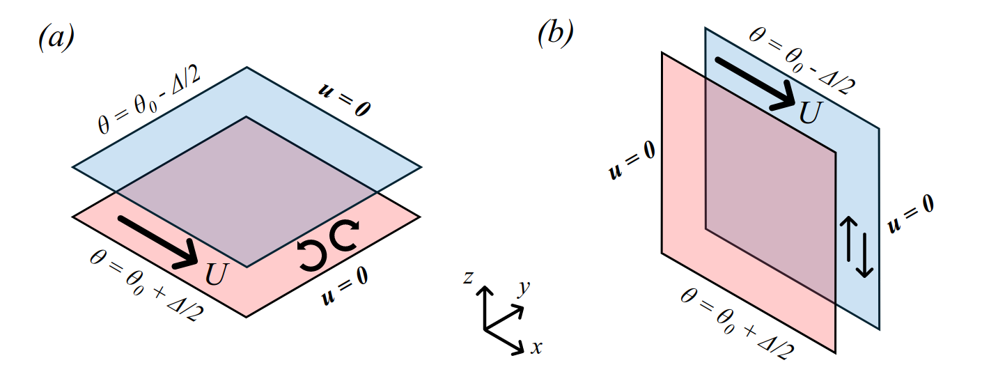
We perform numerical simulations of the flow arising in a fluid confined between two parallel no-slip vertical walls. The walls are separated by a horizontal distance and are held at fixed temperatures, with a temperature difference of between the plates. As in the schematic in figure 1(b), we take the -coordinate to be horizontal and parallel to the plates, the -coordinate to be normal to the boundaries, and to be in the vertical direction. We consider a fluid satisfying the Oberbeck–Boussinesq approximation, such that changes in density are only significant in the buoyancy term and are linear with respect to changes in temperature. We therefore treat the velocity field as divergence-free () and satisfying the Navier–Stokes momentum equation
| (1) |
where is the mean fluid density (assumed constant), is the pressure, is the kinematic viscosity, is the acceleration due to gravity, and is the thermal expansion coefficient. A time-dependent, spatially-uniform forcing is applied in the streamwise () direction to maintain a constant mean flow . Previous work has shown that such a forcing produces near-identical results to those of a constant pressure gradient (Quadrio et al., 2016), but allows us to use the mean flow strength as an input parameter. The temperature field satisfies the advection-diffusion equation
| (2) |
where is the thermal diffusivity. Periodic boundary conditions are applied to both and in the and directions. Unless otherwise stated, the aspect ratio of the domain in these periodic directions is taken as .
We perform direct numerical simulations of equations (1) and (2) using a highly-parallelised flow solver that computes spatial derivatives using second-order central finite differences. The wall-normal diffusive terms are evolved in time using a Crank–Nicolson scheme and all other terms are treated explicitly using a three-stage Runge–Kutta method. The velocity is kept divergence-free using a pressure correction step at each time step. A multiple-resolution technique is applied to evolve the velocity and temperature fields on independent grids, with cubic Hermite interpolation used for the buoyancy forcing and the advection of temperature. Detailed overviews of the numerical discretization, the domain decomposition strategy and the multiple-resolution technique can be found in Verzicco & Orlandi (1996); van der Poel et al. (2015); Ostilla-Monico et al. (2015) as well as in our software documentation.
The physical input parameters of the system are the Rayleigh number, the Prandtl number, and the Reynolds number
| Ra | (3) |
When considering the strength of the flow driven by convection, it is often useful to consider the Grashof number as the relevant input parameter, and when comparing the relative strengths of buoyancy to pressure driving, we can construct a Richardson number as
| (4) |
These can both be considered as input parameters. Above we have written as the free-fall velocity scale to give insight on the interpretation of these parameters.
In this study, we perform two sets of simulations to compare the relative impacts of the various input parameters. Firstly, we fix and vary along with , which correspond to Richardson numbers of . For the second set, we fix and increase Gr up to while again varying up to . A detailed overview of the parameters used for each simulation are given in table 1 of appendix B. Each simulation is run to a statistically steady state, in which the flow statistics are computed and averaged for a minimum of 200 advective time units. For high the relevant time unit is , whereas for low the relevant time unit is . The wall-normal grid spacing is stretched following Pirozzoli & Orlandi (2021) to ensure sufficient resolution close to the wall, such that at the wall for the base velocity grid. In the periodic directions, the uniform grid spacing satisfies in every simulation. At the centre of the domain, the spacing of the refined grid satisfies , , where is the Batchelor scale computed using the plane-averaged TKE dissipation rate over the mid-plane. Full details of the grid sizes are provided in appendix B.
3 Flow visualisation
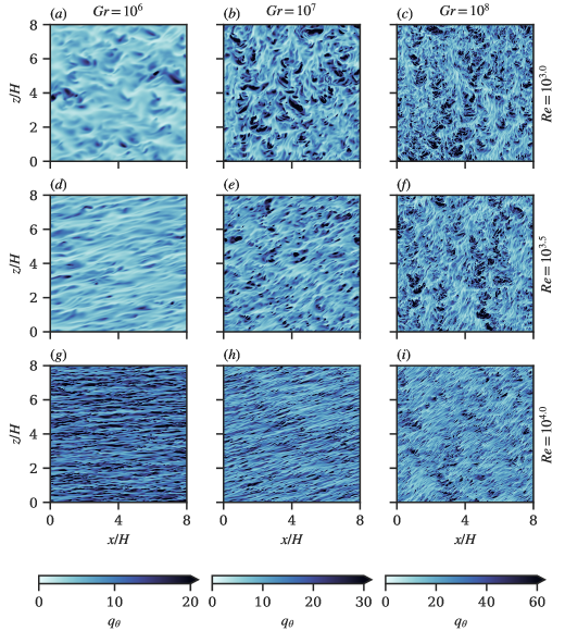
We begin with a qualitative comparison of the simulations through visualisations of the temperature field. Figure 2 displays the instantaneous local wall-normal heat flux at the boundary plate for cases with fixed , and a range of , . The dimensionless heat flux plotted here is defined as
| (5) |
such that its time- and plane-averaged value is equivalent to the Nusselt number, .
As mentioned above, the relative strength of convection to shear forcing can be characterised by the Richardson number , which is constant along diagonals in figure 2. At high , as in panel , the horizontal shear has little impact on the local distribution of the wall heat flux. The near-wall temperature structures are the same as the case in the absence of shear, with regions of large local heat flux (dark spots) separated by longer, streaky structures aligned in the vertical (Howland et al., 2022). As decreases, such as in panels and where , the prominence of the large heat flux regions diminishes and the streaks become aligned in the diagonal. This visualises the local direction of the flow along the wall, which at is due to a combination of the vertical convection and the horizontal pressure gradient. At lower , these structures become more aligned with the horizontal, eventually spanning the domain as in panel , which is reminiscent of classical low-speed streaks in turbulent channel flow (Kline et al., 1967; Antonia et al., 2009). A more quantitative analysis of the change in the near-wall heat flux distribution will be provided in §7.
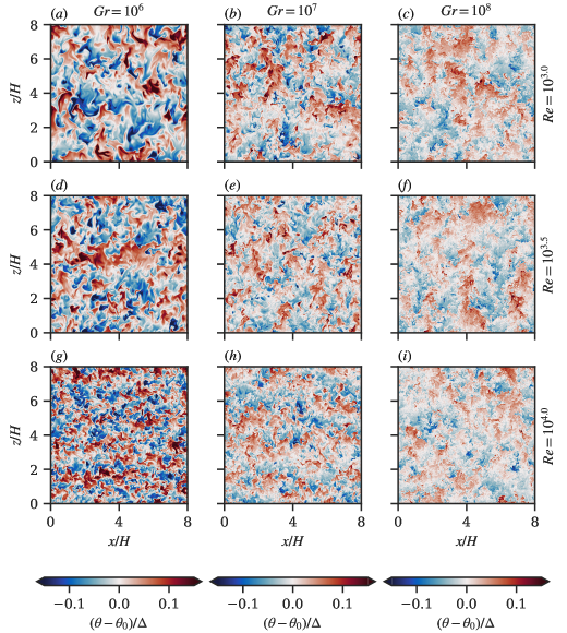
In figure 3, we present visualisations of the same simulations but now at the midplane of the simulation domain . As would be expected, the fields at higher Gr and exhibit structures with a wider range of spatial scales. Aside from this dynamical range, the effect of increasing is less noticeable at the midplane than at the wall in figure 2. At the centre of a turbulent channel, the mean profile of horizontal velocity is relatively flat, with zero mean shear and a local minimum in turbulent kinetic energy. By contrast in vertical convection, a mean shear in the vertical velocity drives the generation of turbulence in the bulk, argued by Li et al. (2023) to follow a mixing layer-like behaviour. In figure 3, greater mixing at higher Gr leads to smaller values of the temperature perturbations in the midplane, although the same effect is not evident as increases. Compared to the mixed Rayleigh–Bénard system, where gravity is orthogonal to the plates and the temperature field organises into large, streamwise-aligned coherent rolls, the fields in mixed VC appear rather featureless. A hint of such large-scale rolls is only noticeable for the cases dominated by strong shear driving with high and low Ri (panels ) where the temperature structures appear more aligned along the streamwise () axis. This contrast in the organisation of mixed convection systems will be investigated more quantitatively in §6 through spectral analysis, but we first turn to the global responses of the two mixed convection systems in the next section.
4 Global response quantities in mixed convection systems
In this section, we compare the responses of the mixed vertical convection setup with those of mixed Rayleigh–Bénard using the simulation data of Yerragolam et al. (2024). Those simulations cover a comparable range of parameters of , , and in a domain of streamwise aspect ratio and spanwise aspect ratio . The flow solver shares an identical code base except for the multiple-resolution technique, which is only used in the newly reported mixed VC simulations.
4.1 Friction coefficients
A key global response parameter in shear-driven flows is the friction coefficient
| (6) |
where is the wall shear stress and is the velocity magnitude in the bulk. Since the friction coefficient is solely determined by the velocity field, we can expect a relationship independent of the Prandtl number. Power-law scalings for can be derived for laminar boundary layer flows, with for example applicable to Couette or Poiseuille flows and arising from the classical Blasius boundary layer solution (Schlichting & Gersten, 2016). For a turbulent boundary layer in the sense of Prandtl and von Kármán, the friction coefficient satisfies the relation
| (7) |
known as the Prandtl friction law after Prandtl (1932). The von Kármán constant typically takes a value around 0.4 and the intercept close to 4 but the exact values, their universality and the way in which they are fit to data remain an active topic of research (Monkewitz & Nagib, 2023). Due to our similar setup and numerical methods, we take the values suggested by Pirozzoli et al. (2014) of and .
Since the mixed VC flow is driven in orthogonal directions by the pressure gradient and by buoyancy, we can construct separate friction coefficients for each component of the wall shear stress. Understanding the response of the friction coefficients in this context relies on choosing an appropriate Reynolds number for each component of the flow. For the streamwise () direction in which the mean flow is imposed by a pressure gradient, this Reynolds number is simply the input parameter defined in (3).
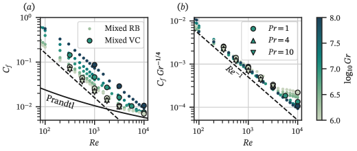
We consider the response of the streamwise friction coefficient in figure 4, where only the streamwise component of the shear stress is applied to the definition (6). The global response of mixed VC is near-identical to that of mixed RB, with a transition from a laminar power-law scaling to the Prandtl friction law of (7). In the laminar scaling regime, stronger buoyancy driving (characterised by higher Gr) leads to an increase in the streamwise skin friction for a given . This in turn delays the transition to the ‘fully turbulent’ Prandtl friction law (7) to higher . Unlike in standard Poiseuille or Couette flow, where a subcritical transition arises due to instability of the laminar base flow and leads to a jump in , the streamwise boundary layer transition in mixed convection systems appears smooth. At low , although the relationship exhibits a laminar-like scaling, one should recall that the convection flow in the interior remains turbulent. In figure 4b, we focus on clarifying this low regime and the increase in with stronger convection. Across both mixed convection systems and for a range of , we find a collapse of the data upon rescaling by . The scaling that arises from laminar profiles in Couette/Poiseuille flow, appears somewhat too steep to accurately describe the data. Blass et al. (2020) reported a scaling of in Couette–Rayleigh–Bénard, but at this time there is no theoretical basis for such a scaling. Note that one could equivalently express the simplified collapse as using the definitions of (4). In the case of mixed convection, non-zero Reynolds stresses in the equation for the mean profile can be expected to modify the mean momentum budget, which shall be analysed later for mixed VC in §5.
We now turn to the friction coefficient associated with the buoyancy-driven component of the flow. For the mixed VC system, we can simply take the peak velocity of the mean vertical velocity as the relevant velocity scale and directly measure the mean vertical shear stress at the wall . In the Rayleigh–Bénard configuration, the convection has no preferential direction along the walls, resulting in zero mean shear stress. However, we can still construct a friction coefficient associated with the persistent large-scale circulation by using the root-mean-squared (RMS) horizontal velocity profile . When shear is added to the RB system, the large-scale circulation aligns itself perpendicular to the imposed shear (Pirozzoli et al., 2017; Yerragolam et al., 2022), so for the mixed RB cases we construct a friction coefficient using only the spanwise RMS velocity. Defining the friction coefficient in this way will only be appropriate for cases where the convectively-driven flow is stronger than the spanwise velocity fluctuations induced by the turbulent shear flow, that is for .
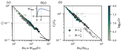
In terms of the Reynolds number, the plate separation is no longer the appropriate length scale for describing the boundary layer dynamics of the convectively-driven flow. As shown in the inset of figure 5a, the mean profile of the vertical velocity in (mixed) VC reaches its peak value at a certain wall-normal distance . From this, we can define a boundary layer Reynolds number
| (8) |
that drives the behaviour at the wall. We construct an analogous Reynolds number for the mixed Rayleigh–Bénard system using the spanwise RMS velocity profile. The friction coefficients of the convective flow component are plotted against in figure 5. Note that is not known a priori but is itself a response parameter of the system that varies with Gr, , and . Similar to the low regime for the streamwise friction, we observe a power-law scaling close to .
This is made clearer in figure 5b, where we collapse the data using the friction coefficient and Reynolds number obtained from the corresponding natural convection flows, matching and . Deviations from the scaling relation are observed for cases where , highlighted by translucent symbols in the figure. As mentioned above, for the mixed RB system this is likely an artefact of using the spanwise RMS velocity to construct the friction coefficient. However, we also observe the discrepancy for low in mixed VC, suggesting that at low Richardson numbers the turbulence generated by the imposed horizontal shear disrupts the near-wall vertical velocity. A more in-depth analysis of the mean vertical momentum budget in mixed VC will be presented in §5.
4.2 Nusselt number
The dimensionless heat flux through the system is characterised by the Nusselt number, defined as
| Nu | (9) |
Here is the horizontal heat flux through the system (normalised by the specific heat ), and the overbar denotes averaging in time and in directions parallel to the plates. Integration of the mean temperature equation (5) shows that is constant across the domain in a statistically steady state.
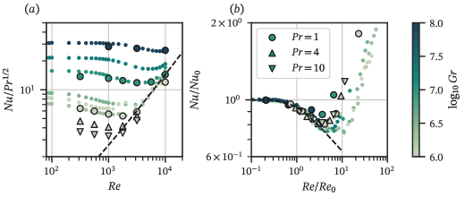
In figure 6, we plot the Nusselt number compensated by . This pre-factor seems appropriate for the -dependence of passive scalar transport in turbulent boundary layers when (Kays et al., 2005), although at higher one expects a transition towards a dependence (Kader & Yaglom, 1972; Alcántara-Ávila & Hoyas, 2021). The data of both systems converge towards the expression
| (10) |
where follows the Prandtl law of (7). This expression draws a parallel between the transport of heat and momentum at the wall, known as the Reynolds analogy, and describes the heat transport in ‘forced convection’ when buoyancy no longer affects the flow. At low (or more precisely high ), the Nusselt number responses of the two systems (VC and RB) do not match as precisely as the friction coefficients. Indeed, in the absence of an external flow, VC and RB do not exhibit the same response due to the lack of coupling between the kinetic energy budget and the heat flux in VC (Ng et al., 2015).
However, we observe a more universal behaviour when the Nusselt numbers in the mixed convection systems are normalised by the values for the equivalent natural convection systems . In figure 6, the normalised Nusselt numbers are plotted as a function of the input Reynolds number normalised by the Reynolds number of the natural convection case . For the mixed VC cases, we define as the peak velocity of the natural VC flow as highlighted in the inset of figure 5. For mixed RB, we follow Yerragolam et al. (2024) in using the volume-averaged RMS velocity for , and note that the results are insensitive to this choice of velocity scale in describing the ‘wind’ of the large-scale circulation. For , all the data from both configurations collapse onto a single curve, showing a drop in the heat flux of up to 25%. Yerragolam et al. (2024) provide an estimate for this drop, derived from the kinetic energy balance in mixed Rayleigh–Bénard, but this balance cannot be related to the horizontal heat flux that is relevant for mixed VC.
In summary, in this section we have demonstrated the universality in the global response parameters of mixed RB and mixed VC, namely in the friction coefficient and the Nusselt number, and the limitations of this universality. In the following sections, we will compare more local quantities, starting with the wall-normal profiles.
5 Wall-normal profiles in mixed vertical convection
We now turn to the first and second order statistics, averaged parallel to the plates, to further investigate the dynamics behind the observed global responses. For clarity, we focus solely on the new simulations of mixed vertical convection and study the variation across the three-parameter space of Gr, and .
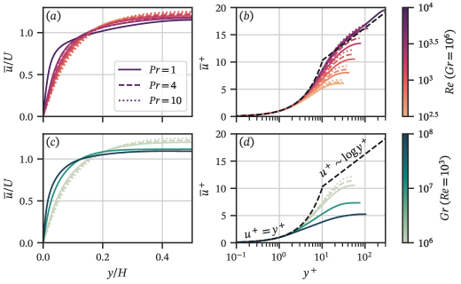
We begin with the response of the mean streamwise velocity in figure 7. For a fixed , as in panels -, the effect of increasing can be seen most clearly when the mean velocity profiles are scaled by viscous wall units in figure 7. As increases, the velocity profile tends towards the classical log-law profile, with the case of closely matching the profile of turbulent Poiseuille flow from Lee & Moser (2015). The effect of stronger thermal convection on the mean profile is also similar to that observed in other mixed convection systems in the literature. In figure 7, where is fixed and Gr varies between and , higher Gr leads to a flatter mean profile in the bulk of the channel. This is illustrated further in wall units in figure 7, where a significant drop in is observed for . Plus symbols denote scaling in viscous wall units with velocity and length . Such a drop is consistent with the previous findings of Scagliarini et al. (2015) for mixed Rayleigh–Bénard, who proposed a modified log-law based on mixing length arguments coupled to the temperature field.
Further insight for the streamwise velocity can be gained from the appropriate component of the Reynolds stress. Considering a statistically steady state, we average the streamwise component of the momentum equation (1) to obtain
| (11) |
where an overbar denotes an average in the periodic (, ) directions and in time. From volume-averaging, we can also relate the mean pressure gradient forcing to the mean wall shear stress through . The first integral of (11) can therefore be written as
| (12) |
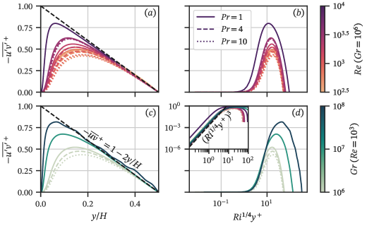
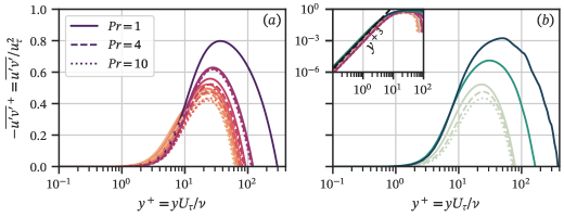
From (11)-(12), the close coupling of the mean streamwise velocity and the Reynolds stress is evident. We therefore present the profiles of in figure 8. As expected, the Reynolds stress dominates the viscous contribution to (12) away from the walls, leading to a balance of as shown in panels and . Relative to , the boundary layer in which the viscous term is relevant becomes thinner as both and Gr increase. The near-wall behaviour of exhibits a remarkable collapse when scaled by as in panels and of figure 8, except for the highest case with .
The additional factor suggests that the appropriate near-wall length scale for the Reynolds stress is modified from the standard viscous wall unit as
| (13) |
The additional pre-factor of in front of the shear stress suggests that the vertical, convectively-driven component of shear cannot be neglected when considering the streamwise Reynolds stress. An improved collapse to that seen in figure 8 can be found by computing a viscous length scale using the total shear stress at the wall . As explicitly shown in appendix A, with this scaling the Reynolds stress for the highest case also matches the other curves. The presence of the convectively-driven flow increases the near-wall Reynolds stress, which in turn leads to the flattened mean velocity profiles observed in figure 7d.
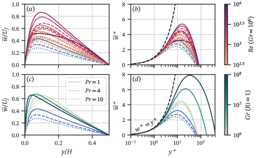
The effect of convection on the shear is by no means a one-way interaction. This is evident from the modification of the mean vertical velocity profile by the imposed horizontal flow. In figures 9, vertical velocity profiles are shown for fixed and varying , with the reference natural convection case () highlighted in blue for comparison. Compared to the natural VC case, the introduction of horizontal driving at moderate leads to an increase in the peak vertical velocity, and hence an increase in the mean shear both in the bulk and at the walls. At the highest (the darkest red line in figure 9), a subsequent decrease is observed in the peak vertical velocity, as well as a nonlinear profile in the bulk. None of the cases studied here exhibit a log-layer in the vertical velocity, with the largest being approximately 6.5 for the most strongly convective case of . For fixed (shown in figures 9), all cases show a similar increase in the peak velocity, and the mean gradient in the bulk appears largely independent of Gr and . The distance of the velocity peak from the wall (compared to the channel width ) decreases for larger Gr, but the value of the peak velocity in free-fall units does not strongly depend on Gr. This similarity at constant is suggestive that the vertical velocity modification is primarily determined by the relative strength of shear driving to convection.
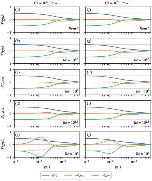
To further investigate the behaviour of the vertical velocity profiles, we now turn to the mean vertical momentum budget. Unlike the streamwise velocity in (11)-(12), the vertical velocity is not only tied to the Reynolds stress profile. Rather, the mean vertical momentum equation reads
| (14) |
Close to the wall, we expect the Reynolds stress to be negligible and a balance to arise between buoyancy and viscosity. Due to the symmetry of the boundary conditions, all three terms must be zero at the channel centre. In the bulk of the flow, the mean velocity is approximately linear, so we expect a balance between buoyancy and Reynolds stress. These features are present in each of the simulations highlighted in figure 10. As increases, the key modification to the budget arises in the Reynolds stress term . In natural VC, there is a miniscule positive peak in the Reynolds stress term close to the wall, but its amplitude is so small that it is indistinguishable in figures 10. This peak grows with , becoming visible at in panels , coinciding with a flattened profile of the viscous term (shown in green). By , at which the Reynolds stresses are significantly energised by the horizontal shear forcing, the nonlinear term peak exceeds the contribution from the buoyancy term. This leads to a significant drop in the viscous term around , which determines the modified mean velocity observed in figure 9.
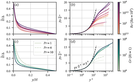
Changes in the mean temperature profile in figure 10 are more subtle, with the most obvious feature being a slight drop in panel , coinciding with the Reynolds stress peak. A clearer picture of the mean temperature response can be found in figure 11, where profiles are plotted both on linear axes and in wall units. Since the dimensionless wall temperature gradient is equivalent to the Nusselt number, which is most strongly dependent on , we compare the temperature profiles in panels at varying and but fixed . As shown in these panels, the temperature gradient in the bulk increases with , and any possible log-law profile does not collapse to a universal slope or coefficient. For fixed however, shown in figure 11, the bulk gradient appears independent of Gr, suggesting that and are the key control parameters determining the flow properties away from the walls.
6 Spectral analysis
We now investigate the scale-dependence of the thermal structures and heat flux in mixed convection through analysis of the power spectra. To ensure that we capture the full range of dynamical scales, we perform further simulations in extended aspect ratio domains, with . The details of these simulations are outlined in table 2 of appendix B.
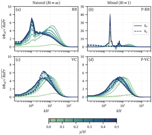
In unsheared Rayleigh–Bénard convection, Krug et al. (2020) show that large-scale patterns, also known as superstructures, can be identified from a low-wavenumber peak in the power spectrum of the temperature field and in the co-spectrum of the wall-normal heat flux. This peak denotes the scale of the large-scale circulation or ‘wind’ of convection key to theories describing RBC. Since there is no preferential horizontal flow direction in RBC, one-dimensional spectra can be analysed, but in mixed and vertical convection, the two directions parallel to the plates must be considered separately.
We therefore compute time-averaged spectra using two-dimensional Fourier transforms in the periodic directions. For visualisation purposes, we present separate one-dimensional spectra for the streamwise () and spanwise () wavenumbers, which are computed by integrating over the other wavenumber. Precisely, the two- and one-dimensional co-spectra of any two variables and are defined as
| (15) |
where denotes the two-dimensional Fourier transform of in and , is the real part. The Fourier transforms are normalised such that integrating the spectrum over wavenumber space recovers the corresponding volume-averaged quantity .
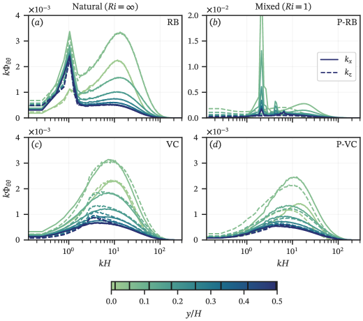
The power spectrum of temperature is presented in figure 12 for the four extended simulations. In panel , for the standard RB configuration, we see similar behaviour to Krug et al. (2020), with a distinct, sharp low wavenumber peak at , and a more broad peak at smaller scales. As mentioned above, the lack of a preferential direction means that the two directional spectra are virtually identical. When shear is added to the RB system in panel , the horizontal isotropy in the system is destroyed. As expected from previous work on mixed RB (Pirozzoli et al., 2017; Blass et al., 2020, 2021; Yerragolam et al., 2022), coherent rolls aligned with the streamwise axis dominate the signal. Note the difference in -axis between figures 12 and 12. In the streamwise spectrum a sharp peak at is visible at all wall-normal locations, but is particularly prominent in the near-wall region (light green) where there is a maximum in (Pirozzoli et al., 2017). The corresponding wavelength of these structures is , which is consistent with that observed previously in the mixed convection literature at . The alignment of the flow structures in the streamwise direction leads to a broad contribution to the streamwise spectrum at low . This behaviour is purely a result of the regular alignment, and is not related to any domain size effects.
In figures 12, we present the same analysis but for natural and mixed vertical convection. The contrast to the RB cases is immediately apparent, with no sharp peaks at any wavenumber or wall-normal position. This confirms the earlier visual observation of figure 3, where the instantaneous snapshots showed no clear coherent length scale. In natural VC, shown in figure 12, the two 1-D spectra do not overlap exactly like in the RB case due to the buoyancy-driven mean flow in the vertical. The spectrum shows a small peak around that is absent from the spectrum, and becomes more prominent towards the channel centre. Comparing figures 12 and 12, we see that this peak is suppressed by the addition of external shear. Furthermore, all of the broad mid-range peaks in the spectra exhibit a decrease in amplitude and a shift to higher wavenumbers.
The heat flux cospectra , shown in figure 13, exhibit similar features to the power spectra. In panels and , a sharp low-wavenumber peak is once again visible for RB and mixed RB systems, and for the heat flux this peak increases towards the channel centre. A broad, high-wavenumber peak is also observed in the spectrum close to the wall. This peak flattens and shifts to lower wavenumbers (i.e. larger scales) as distance from the wall increases, which can be interpreted as the emergence and coalescence of small-scale plume structures. A similar behaviour can be found in the VC configurations of panels and , with the broad peak in both and spectra shifting to lower wavenumbers for larger . However, in the spectrum for natural VC (where is perpendicular to gravity), this peak also increases in amplitude towards the channel centre, highlighting that the majority of the wall-normal heat transport at the channel centre occurs due to structures of size . Comparing this to the mixed VC case in figure 13, the mid-scale peak appears significantly suppressed when the external shear is imposed, suggesting that the coalescence of plumes in the bulk is disrupted by the shear. This is consistent with the interpretation of Domaradzki & Metcalfe (1988) and Scagliarini et al. (2014) who argued that the drop in heat flux in mixed RB can be related phenomenologically to disruption of the organisation of small-scale convective plumes.
7 Boundary layer statistics
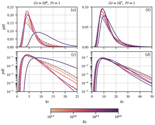
Whereas the previous section focused on the advective heat flux in the bulk and its modification due to shear, we now turn to the conductive heat flux that dominates the transport in the boundary layer. Specifically, we investigate the statistical distribution of the local conductive heat flux at the boundary plates. As defined earlier in (5), we consider the local dimensionless heat flux whose time- and plane-average is equivalent to the Nusselt number. The pointwise data of , also shown in figure 2, is collected over time and space to construct histograms that are normalised to produce probability density functions in figure 14. The data shown here is only for and since these cases cover the widest range of Richardson number, highlighting the transition from natural convection to forced convection.
In figure 14, where the data are presented on linear axes, we find the same effect of increasing shear at both Grashof numbers. As increases from zero (shown by progressively darker lines, with marked in blue for comparison) the peak of the pdf increases in amplitude. In statistical terms, this means that the most common values of local heat flux become more common as shear is increased, up to . Due to the skewed nature of the distributions, these increasingly common values of heat flux are below the mean, and although the peak shifts slightly to the right as increases, these parameters are associated with the drop in heat flux observed in figure 6. This corresponds to the visualisation of figure 2, where the streaks of low heat flux span a larger proportion of the boundary at (panels e,i) than at high (panels b,c). Once is sufficiently high, which in these cases is for , the whole distribution shifts more significantly to higher as the transport becomes dominated by shear driving.
At moderate , another key modification is to the tails of the distribution. These are most clearly visualised in figure 14, where the heat flux distributions are plotted on a logarithmic axis. In this representation, it is clear that the right tails of large heat flux decay exponentially for , and close to exponentially for . At both Grashof numbers, the tails are reduced as increases relative to the natural convection case, showing that the probability of extreme local heat flux values is reduced due to the introduction of a mean horizontal flow. Again, this is consistent with what was observed in the visualisation of figure 2, where dark patches associated with large local heat flux became less prevalent as increases. In natural VC, Pallares et al. (2010) used conditional sampling to show that these patches are most often associated with instantaneous flow reversals at the walls, which are likely a result of impacting plumes originating from the opposing wall.
8 Conclusion and outlook
In this paper, we have investigated mixed convection in a differentially heated vertical channel subject to a horizontal pressure gradient, referred to as mixed VC, through direct numerical simulations. By simulating the system across the parameter range , , and , we have explored the transition from natural convection to forced convection, characterised by the Richardson number . Across this parameter range, the response of the streamwise skin friction is identical to the response seen in mixed Rayleigh–Bénard (RB) convection, with a power-law -dependence for giving way to the Prandtl friction law (7) at sufficiently high . The presence of convection acts to increase the skin friction for a given , due to the thermal plumes emitted from the plates, with a collapse observed for all the data in the power-law regime of for both configurations across the entire range of . For mixed VC, the streamwise momentum budgets show an enhanced impact of Reynolds stresses close to the wall at higher , which modify the shape of the mean velocity profile. The Reynolds stresses in the boundary layer are driven by the combined shear stress of the horizontal pressure-driven flow and the vertical convection flow.
Friction coefficients could also be obtained for the flow component associated with buoyancy driving. For cases with significant buoyancy effects at , a reasonable collapse was found for the laminar-like scaling where is the boundary layer Reynolds number of the convection flow. The introduction of the horizontal pressure gradient leads to significant modification of the mean vertical velocity, with increasing up to three times its value for natural convection, and a corresponding increase in the mean shear in the channel bulk for moderate . For , the response of the Nusselt number Nu to the introduction of shear in mixed VC is also identical to that in mixed RB. Before the flow undergoes a transition to a forced convection regime at high , the response can be expressed as where and are the Nusselt number and Reynolds number associated with natural convection. The data of both mixed convection systems collapse onto this single curve, which describes the drop in Nu as increases.
The near identical quantitative response of mixed RB and mixed VC is observed despite striking qualitative differences between the two configurations in terms of large-scale flow organisation. Whereas mixed RB features large convective rolls oriented along the streamwise axis, no such structures form in mixed VC except at low when the dynamics are solely dominated by the shear forcing. The absence of a low wavenumber peak in the heat flux co-spectrum for mixed VC confirms that the advective heat flux across the domain is transported by eddies or plumes with a wide range of scales rather than by large coherent rolls. Comparing the spectra from natural VC with mixed VC reveals that the organisation of plume structures with a horizontal scale of is suppressed by the horizontal mean flow. This is reflected also in the distribution of local heat flux at the boundaries, which shows that instantaneous events of extreme heat flux become less likely as increases. As the boundaries becomes dominated by streaky structures, the formation of localised plume structures is disrupted, consistent with the earlier interpretations of reduced heat flux in mixed RB (Domaradzki & Metcalfe, 1988; Scagliarini et al., 2014).
The striking agreement between the two channel configurations compared here, regardless of the gravity direction, opens up the question of how universal such a response in skin friction and heat flux is for other mixed convection systems. The independence to the gravity direction suggests that our results may be applicable more generally to inclined layer convection, as studied by Daniels & Bodenschatz (2002) at low , subject to a horizontal pressure gradient at comparable Gr and . However, it is less clear how directly applicable the findings here are to a wall plume subject to a crossflow. Such a scenario is relevant to environmental applications such as at a melting ice face subject to ambient ocean currents (Jackson et al., 2020). Whereas both boundaries impact the transport in mixed RB and mixed VC, a wall plume constantly entrains fluid from the ambient at its outer edge. Recent work has provided an innovative way to simulate wall plumes at high Gr, through studying temporally-growing boundary layers (Ke et al., 2023; Wells, 2023), and it would be fruitful to understand how the growth of these boundary layers is affected by the presence of a turbulent crossflow. For ice-ocean interactions, the picture is further complicated through multicomponent transport (Howland et al., 2023) and the development of rough boundaries which are closely coupled to the flow structures (Couston et al., 2021; Ravichandran et al., 2022).
From a more theoretical standpoint, our current work has also emphasised how certain flow properties are noticeably modified under the transition from natural vertical convection to forced convection. These include the sign of the near-wall Reynolds stress in figure 10 and the distribution of the local wall heat flux in figure 14. In both RB and VC, predictions have been made for a transition to the ‘ultimate’ regime at sufficiently high buoyancy driving, where the boundary layers behave as turbulent boundary layers (Lohse & Shishkina, 2023), although this regime has thus far been inaccessible to three-dimensional numerical simulation. Analysis of the aforementioned statistical quantities in natural convection at high Gr may help in identifying key markers of such a transition in natural convection systems.
[Acknowledgements] We are grateful to Emily Ching for fruitful discussions about natural vertical convection and to Olga Shishkina and Richard Stevens for insights into the response of mixed Rayleigh–Bénard convection.
[Funding] The work of CJH was funded by the Max Planck Center for Complex Fluid Dynamics. The contribution of GSY towards this project has received funding from the European Research Council under the European Union’s Horizon 2020 research and innovation program (Grant No. 804283). We acknowledge PRACE for awarding us access to Irene at Très Grand Centre de Calcul (TGCC) du CEA, France (project 2021250115). For the extended domain simulations, the authors also gratefully acknowledge the Gauss Centre for Supercomputing e.V. (www.gauss-centre.eu) for funding this project (pr74sa) by providing computing time on the GCS Supercomputer SuperMUC-NG at Leibniz Supercomputing Centre (www.lrz.de). This work was also carried out on the Dutch national e-infrastructure with the support of SURF Cooperative.
[Declaration of interests]The authors report no conflict of interest.
[Author ORCIDs]
Christopher J. Howland https://orcid.org/0000-0003-3686-9253;
Guru Sreevanshu Yerragolam https://orcid.org/0000-0002-8928-2029;
Roberto Verzicco https://orcid.org/0000-0002-2690-9998;
Detlef Lohse https://orcid.org/0000-0003-4138-2255.
Appendix A Alternative near-wall scaling for the streamwise Reynolds stress
As shown in figure 8, the near-wall profile of the streamwise Reynolds stress requires an additional prefactor of to collapse the majority of the cases studied here. In §5, we attribute this to the multiple components of shear at the wall that produce the Reynolds stress, which cannot be captured by the streamwise component alone. This is confirmed in figure 15, where we re-plot against a wall-normal coordinate scaled with the total shear stress at the wall. Specifically, we scale with the viscous wall unit where the total friction velocity satisfies
| (16) |
Compared to the results of figure 8, the previously outlying case of (plotted as a dark purple line) now also shows a reasonable collapse with the rest of the data in the near wall region of figure 15. This result highlights the intricate nature of turbulence in mixed vertical convection, with different friction velocities needed to scale the two axes of figure 15 to describe the Reynolds stress. Although the near-wall length scale is determined by the total shear stress in (16), the Reynolds stress must still satisfy the global balance (12), where is the relevant velocity scale.
Appendix B Simulation parameters
Table 1 details the physical and numerical input parameters used for the mixed vertical convection simulations. Even at , we use a more refined grid for the temperature field since sharper gradients can emerge than in the velocity field due to the lack of a pressure gradient term in (2) when compared with (1).
In §6, an additional set of simulations are discussed in which the periodic extent of the domain is tripled to an aspect ratio of . In that section, we compare RB configurations with gravity aligned normal to the boundary plates (in the negative direction) to VC configurations where gravity is aligned parallel to the plates (in the negative direction). Table 2 details the input parameters used for these additional simulations. Note that a prefix of ‘P-’ in the name of the simulation denotes the presence of a Poiseuille-like pressure gradient forcing.
| 1 | 512 | 192 | 1024 | 384 | 36.8 | 6.37 | ||||
| 1 | 512 | 192 | 1024 | 384 | 48.8 | 5.98 | ||||
| 1 | 512 | 192 | 1024 | 384 | 61.1 | 5.57 | ||||
| 1 | 512 | 192 | 1024 | 384 | 81.6 | 5.33 | ||||
| 1 | 768 | 192 | 1536 | 384 | 85.2 | 5.85 | ||||
| 1 | 1024 | 192 | 2048 | 384 | 43.2 | 12.01 | ||||
| 4 | 512 | 192 | 1024 | 384 | 29.9 | 9.39 | ||||
| 4 | 512 | 192 | 1024 | 384 | 41.3 | 8.69 | ||||
| 4 | 512 | 192 | 1024 | 384 | 59.6 | 8.15 | ||||
| 4 | 512 | 192 | 1024 | 384 | 74.6 | 8.39 | ||||
| 4 | 768 | 192 | 1536 | 384 | 61.3 | 10.46 | ||||
| 10 | 512 | 192 | 1536 | 576 | 28.7 | 11.48 | ||||
| 10 | 512 | 192 | 1536 | 576 | 39.7 | 10.73 | ||||
| 10 | 512 | 192 | 1536 | 576 | 58.2 | 10.38 | ||||
| 4 | 512 | 192 | 1536 | 576 | 76.9 | 8.42 | ||||
| 10 | 768 | 192 | 2304 | 576 | 45.3 | 15.04 | ||||
| 1 | 512 | 192 | 1024 | 384 | 90.3 | 13.74 | ||||
| 1 | 512 | 192 | 1024 | 384 | 99.8 | 13.14 | ||||
| 1 | 512 | 192 | 1024 | 384 | 118.9 | 12.47 | ||||
| 1 | 768 | 192 | 1536 | 384 | 136.7 | 11.85 | ||||
| 1 | 768 | 192 | 1536 | 384 | 157.9 | 12.06 | ||||
| 1 | 1024 | 256 | 2048 | 512 | 160.6 | 14.39 | ||||
| 1 | 1536 | 384 | 2304 | 512 | 198.0 | 28.14 | ||||
| 1 | 1536 | 384 | 2304 | 512 | 226.7 | 27.05 | ||||
| 1 | 1536 | 384 | 2304 | 512 | 266.6 | 25.82 |
| Name | |||||||||||
|---|---|---|---|---|---|---|---|---|---|---|---|
| RB | 1 | 2304 | 192 | 4608 | 384 | - | 45.0 | 15.79 | |||
| VC | 1 | 2304 | 192 | 4608 | 384 | - | 89.9 | 13.80 | |||
| P-RB | 1 | 2304 | 192 | 4608 | 384 | 70.7 | 12.01 | ||||
| P-VC | 1 | 2304 | 192 | 4608 | 384 | 134.1 | 11.86 |
References
- Alcántara-Ávila & Hoyas (2021) Alcántara-Ávila, F. & Hoyas, S. 2021 Direct numerical simulation of thermal channel flow for medium–high Prandtl numbers up to Re=2000. Int. J. Heat Mass Tran. 176, 121412.
- Antonia et al. (2009) Antonia, R. A., Abe, H. & Kawamura, H. 2009 Analogy between velocity and scalar fields in a turbulent channel flow. J. Fluid Mech. 628, 241–268.
- Blass et al. (2021) Blass, A., Tabak, P., Verzicco, R., Stevens, R. J. A. M. & Lohse, D. 2021 The effect of Prandtl number on turbulent sheared thermal convection. J. Fluid Mech. 910, A37.
- Blass et al. (2020) Blass, A., Zhu, X., Verzicco, R., Lohse, D. & Stevens, R. J. A. M. 2020 Flow organization and heat transfer in turbulent wall sheared thermal convection. J. Fluid Mech. 897.
- Cheng et al. (2021) Cheng, Y., Li, Q., Li, D. & Gentine, P. 2021 Logarithmic profile of temperature in sheared and unstably stratified atmospheric boundary layers. Phys. Rev. Fluids 6 (3), 034606.
- Ching (2023) Ching, E. S. C. 2023 Heat flux and wall shear stress in large-aspect-ratio turbulent vertical convection. Phys. Rev. Fluids 8 (2), L022601.
- Couston et al. (2021) Couston, L.-A., Hester, E., Favier, B., Taylor, J. R., Holland, P. R. & Jenkins, A. 2021 Topography generation by melting and freezing in a turbulent shear flow. J. Fluid Mech. 911.
- Daniels & Bodenschatz (2002) Daniels, K. E. & Bodenschatz, E. 2002 Defect Turbulence in Inclined Layer Convection. Phys. Rev. Lett. 88 (3), 034501.
- Domaradzki & Metcalfe (1988) Domaradzki, J. A. & Metcalfe, R. W. 1988 Direct numerical simulations of the effects of shear on turbulent Rayleigh-Bénard convection. J. Fluid Mech. 193, 499–531.
- El-Samni et al. (2005) El-Samni, O. A., Yoon, H. S. & Chun, H. H. 2005 Direct numerical simulation of turbulent flow in a vertical channel with buoyancy orthogonal to mean flow. Int. J. Heat Mass Tran. 48 (7), 1267–1282.
- Foken (2006) Foken, T. 2006 50 Years of the Monin–Obukhov Similarity Theory. Bound-Lay. Meteorol 119 (3), 431–447.
- Gage & Reid (1968) Gage, K. S. & Reid, W. H. 1968 The stability of thermally stratified plane Poiseuille flow. J. Fluid Mech. 33 (1), 21–32.
- Grossmann & Lohse (2000) Grossmann, S. & Lohse, D. 2000 Scaling in thermal convection: A unifying theory. J. Fluid Mech. 407, 27–56.
- Grossmann & Lohse (2001) Grossmann, S. & Lohse, D. 2001 Thermal Convection for Large Prandtl Numbers. Phys. Rev. Lett. 86 (15), 3316–3319.
- Guo & Prasser (2022) Guo, W. & Prasser, H.-M. 2022 Direct numerical simulation of turbulent heat transfer in liquid metals in buoyancy-affected vertical channel. Int. J. Heat Mass Tran. 194, 123013.
- Howland et al. (2022) Howland, C. J., Ng, C. S., Verzicco, R. & Lohse, D. 2022 Boundary layers in turbulent vertical convection at high Prandtl number. J. Fluid Mech. 930, A32.
- Howland et al. (2023) Howland, C. J., Verzicco, R. & Lohse, D. 2023 Double-diffusive transport in multicomponent vertical convection. Phys. Rev. Fluids 8 (1), 013501.
- Jackson et al. (2020) Jackson, R. H., Nash, J. D., Kienholz, C., Sutherland, D. A., Amundson, J. M., Motyka, R. J., Winters, D., Skyllingstad, E. & Pettit, E. C. 2020 Meltwater Intrusions Reveal Mechanisms for Rapid Submarine Melt at a Tidewater Glacier. Geophys. Res. Lett. 47 (2), e2019GL085335.
- Kader & Yaglom (1972) Kader, B. A. & Yaglom, A. M. 1972 Heat and mass transfer laws for fully turbulent wall flows. Int. J. Heat Mass Tran. 15 (12), 2329–2351.
- Kader & Yaglom (1990) Kader, B. A. & Yaglom, A. M. 1990 Mean fields and fluctuation moments in unstably stratified turbulent boundary layers. J. Fluid Mech. 212, 637–662.
- Kasagi & Nishimura (1997) Kasagi, N. & Nishimura, M. 1997 Direct numerical simulation of combined forced and natural turbulent convection in a vertical plane channel. Int. J. Heat Fluid Fl. 18 (1), 88–99.
- Kays et al. (2005) Kays, W. M., Crawford, M. E., Weigand, B. & Kays, W. M. 2005 Convective Heat and Mass Transfer, 4th edn. Boston, Mass.: McGraw-Hill Higher Education.
- Ke et al. (2023) Ke, J., Williamson, N., Armfield, S. W. & Komiya, A. 2023 The turbulence development of a vertical natural convection boundary layer. J. Fluid Mech. 964, A24.
- Kline et al. (1967) Kline, S. J., Reynolds, W. C., Schraub, F. A. & Runstadler, P. W. 1967 The structure of turbulent boundary layers. J. Fluid Mech. 30 (4), 741–773.
- Krug et al. (2020) Krug, D., Lohse, D. & Stevens, R. J. A. M. 2020 Coherence of temperature and velocity superstructures in turbulent Rayleigh–Bénard flow. J. Fluid Mech. 887, A2.
- Lee & Moser (2015) Lee, M. & Moser, R. D. 2015 Direct numerical simulation of turbulent channel flow up to $Re_\tau \approx 5200$. J. Fluid Mech. 774, 395–415.
- Li et al. (2023) Li, M., Jia, P., Liu, H., Jiao, Z. & Zhang, Y. 2023 Mean velocity and temperature profiles in turbulent vertical convection. J. Fluid Mech. 977, A51.
- Lohse & Shishkina (2023) Lohse, D. & Shishkina, O. 2023 Ultimate turbulent thermal convection. Phys. Today 76 (11), 26–32.
- Madhusudanan et al. (2022) Madhusudanan, A., Illingworth, S. J., Marusic, I. & Chung, D. 2022 Navier-Stokes–based linear model for unstably stratified turbulent channel flows. Phys. Rev. Fluids 7 (4), 044601.
- Monin & Obukhov (1954) Monin, A. S. & Obukhov, A. M. 1954 Basic laws of turbulent mixing in the surface layer of the atmosphere. Tr. Geofiz Inst SSSR 24 (151), 163–187.
- Monkewitz & Nagib (2023) Monkewitz, P. A. & Nagib, H. M. 2023 The hunt for the Kármán ‘constant’ revisited. J. Fluid Mech. 967, A15.
- Ng et al. (2015) Ng, C. S., Ooi, A., Lohse, D. & Chung, D. 2015 Vertical natural convection: Application of the unifying theory of thermal convection. J. Fluid Mech. 764, 349–361.
- Obukhov (1946) Obukhov, A. M. 1946 Turbulence in an atmosphere with a non-uniform temperature. Bound-Lay. Meteorol. 1, 95–115.
- Orlandi et al. (2015) Orlandi, P., Bernardini, M. & Pirozzoli, S. 2015 Poiseuille and Couette flows in the transitional and fully turbulent regime. J. Fluid Mech. 770, 424–441.
- Ostilla-Monico et al. (2015) Ostilla-Monico, R., Yang, Y., van der Poel, E. P., Lohse, D. & Verzicco, R. 2015 A multiple-resolution strategy for Direct Numerical Simulation of scalar turbulence. J. Comput. Phys. 301, 308–321.
- Pallares et al. (2010) Pallares, J., Vernet, A., Ferre, J. A. & Grau, F. X. 2010 Turbulent large-scale structures in natural convection vertical channel flow. Int. J. Heat Mass Tran. 53 (19), 4168–4175.
- Pirozzoli et al. (2014) Pirozzoli, S., Bernardini, M. & Orlandi, P. 2014 Turbulence statistics in Couette flow at high Reynolds number. J. Fluid Mech. 758, 327–343.
- Pirozzoli et al. (2017) Pirozzoli, S., Bernardini, M., Verzicco, R. & Orlandi, P. 2017 Mixed convection in turbulent channels with unstable stratification. J. Fluid Mech. 821, 482–516.
- Pirozzoli & Orlandi (2021) Pirozzoli, S. & Orlandi, P. 2021 Natural grid stretching for DNS of wall-bounded flows. J. Comput. Phys. 439, 110408.
- Prandtl (1932) Prandtl, L. 1932 Zur turbulenten Strömung in Rohren und längs Platten. In Ergebnisse der aerodynamischen Versuchsanstalt zu Göttingen, , vol. 4, pp. 18–29. Oldenbourg Wissenschaftsverlag.
- Quadrio et al. (2016) Quadrio, M., Frohnapfel, B. & Hasegawa, Y. 2016 Does the choice of the forcing term affect flow statistics in DNS of turbulent channel flow? Eur. J. Mech. B/Fluid 55, 286–293.
- Ravichandran et al. (2022) Ravichandran, S., Toppaladoddi, S. & Wettlaufer, J. S. 2022 The combined effects of buoyancy, rotation, and shear on phase boundary evolution. J. Fluid Mech. 941.
- Richter & Parsons (1975) Richter, F. M. & Parsons, B. 1975 On the interaction of two scales of convection in the mantle. J. Geophys. Res. 80 (17), 2529–2541.
- Scagliarini et al. (2015) Scagliarini, A., Einarsson, H., Gylfason, Á. & Toschi, F. 2015 Law of the wall in an unstably stratified turbulent channel flow. J. Fluid Mech. 781, R5.
- Scagliarini et al. (2014) Scagliarini, A., Gylfason, Á. & Toschi, F. 2014 Heat-flux scaling in turbulent Rayleigh-Bénard convection with an imposed longitudinal wind. Phys. Rev. E 89 (4), 043012.
- Schlichting & Gersten (2016) Schlichting, H. & Gersten, K. 2016 Boundary-Layer Theory, 9th edn. Springer, Berlin, Heidelberg.
- van der Poel et al. (2015) van der Poel, E. P., Ostilla-Mónico, R., Donners, J. & Verzicco, R. 2015 A pencil distributed finite difference code for strongly turbulent wall-bounded flows. Comput. Fluids 116, 10–16.
- Verzicco & Orlandi (1996) Verzicco, R. & Orlandi, P. 1996 A Finite-Difference Scheme for Three-Dimensional Incompressible Flows in Cylindrical Coordinates. J. Comput. Phys. 123 (2), 402–414.
- Wells (2023) Wells, A. J. 2023 From classical to ultimate heat fluxes for convection at a vertical wall. J. Fluid Mech. 970, F1.
- Wetzel & Wagner (2019) Wetzel, T. & Wagner, C. 2019 Buoyancy-induced effects on large-scale motions in differentially heated vertical channel flows studied in direct numerical simulations. Int. J. Heat Fluid Fl. 75, 14–26.
- Yerragolam et al. (2024) Yerragolam, G. S., Howland, C. J., Stevens, R. J. A. M., Verzicco, R., Shishkina, O. & Lohse, D. 2024 Scaling relations for heat and momentum transport in sheared Rayleigh-Bénard convection, arXiv: 2403.04418.
- Yerragolam et al. (2022) Yerragolam, G. S., Verzicco, R., Lohse, D. & Stevens, R. J. A. M. 2022 How small-scale flow structures affect the heat transport in sheared thermal convection. J. Fluid Mech. 944, A1.