Shining Light on Periodic Dominating Sets in Bounded-Treewidth Graphs

Abstract

For the vertex selection problem $(\sigma,\rho)\mathchar 45\relax$DomSet one is given two fixed sets $\sigma$ and $\rho$ of integers and the task is to decide whether we can select vertices of the input graph, such that, for every selected vertex, the number of selected neighbors is in $\sigma$ and, for every unselected vertex, the number of selected neighbors is in $\rho$ [Telle, Nord. J. Comp. 1994]. This framework covers Independent Set and Dominating Set for example.

We extend the recent result by Focke et al. [SODA 2023] to investigate the case when $\sigma$ and $\rho$ are periodic sets with the same period ${\mathrm{m}}\geq 2$, that is, the sets are two (potentially different) residue classes modulo ${\mathrm{m}}$. We study the problem parameterized by treewidth and present an algorithm that solves in time ${\mathrm{m}}^{\textup{{tw}}}\cdot n^{\mathcal{O}(1)}$ the decision, minimization and maximization version of the problem. This significantly improves upon the known algorithms where for the case ${\mathrm{m}}\geq 3$ not even an explicit running time is known. We complement our algorithm by providing matching lower bounds which state that there is no $({\mathrm{m}}-\varepsilon)^{\textup{{pw}}}\cdot n^{\mathcal{O}(1)}$ unless SETH fails. For ${\mathrm{m}}=2$, we extend these bound to the minimization version as the decision version is efficiently solvable.

1 Introduction

Lights Out!—the popular 1995 single-player board game presents the unassuming player with a $5\times 5$ grid of switches and lamps, some or all of them initially turned on, and asks the easy-looking task of turning off all lamps by pressing the switches. The catch is that every switch flips not only the state of its corresponding lamp (from “on” to “off” or vice-versa), but also the states of the lamps neighboring the switch in the grid [BBH21, FY13]. Consult Figure 1(a) for a visualization of a short game sequence.

After playing around a little, a now less-unassuming player observes two things: first, the order in which the switches are pressed does not matter. Second, flipping any switch for a second time undoes the first time it was flipped. Hence, we can describe a solution to an initial configuration as a set of switches that need to be flipped to turn all lights off.

Armed with our insights, we can cast the Lights Out! game as an instance to a generalization of the classical Dominating Set problem. First, for the case that initially all lamps are turned on, given a graph (for Lights Out! a $5\times 5$ grid graph), we wish to select a set of vertices such that the closed neighborhood of every vertex contains an odd number of selected vertices (instead of finding a set of vertices such that every vertex is either selected or is adjacent to a selected vertex). Then, we can easily capture general configurations by artificially flipping the parity of any vertex that correspond to a lamp that is initially turned off. Consult Figures 1(b) and 1(c) for a visualization.

In this work, we study generalized dominating set problems (such as the one arising from Lights Out!). Generalizing the recent results by Focke et al. [FMI⁺23a, FMI⁺23b, FMI⁺23c] to obtain both faster algorithms, and matching lower bounds both for finding any solution and for finding a minimum-size or maximum-size solution. For our running example of Lights Out!, perhaps surprisingly, we obtain an optimal algorithm for computing a shortest sequence to turn all lights off, improving over the naive brute-force approach, which was seemingly the only known method to find a sequence to relieve a struggling player as fast as possible.

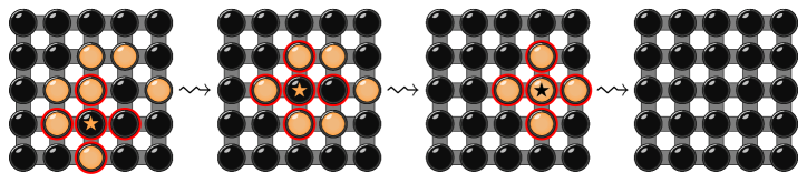
(a) A typical game of Lights Out!. In each turn, the player presses the light marked with a star to flip all encircled lights.

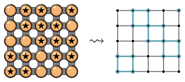
(b) If all lights are turned on initially, any sequence to turn off all lights directly corresponds to a $(\sigma,\rho)$-set in the corresponding graph, where $\sigma$ contains all even numbers and $\rho$ contains all odd numbers. Pressing the lights marked with a star in any order turns all lights off; the corresponding $(\sigma,\rho)$-set is highlighted in the corresponding graph.

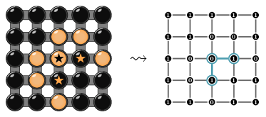
(c) To handle an arbitrary initial state of the game, we keep $\sigma$ and $\rho$ as before, but we add one artificial, always selected vertex to every vertex that corresponds to a light that is initially turned off. (An artificial vertex may itself violate the $\sigma$ and $\rho$ constraints.) In the figure, we denote vertices with such an added artificial vertex by a one inside the vertex.

Figure 1: Lights Out! and the corresponding instances of Generalized Dominating Set visualized.

Understanding Generalized Dominating Set Problems with a Unified Framework.

Already in 1994, Telle introduced the problem (family) $(\sigma,\rho)\mathchar 45\relax$DomSet which is a very general framework for such vertex selection problems with degree constraints [Tel94]. Assume that $\sigma$ and $\rho$ are two fixed, non-empty sets of non-negative integers. For a given input graph $G$, the task is to decide whether there is a vertex set $S\subseteq V(G)$ such that (1) for all $v\in S$, the number of selected neighbors is in $\sigma$, that is, $\lvert N(v)\cap S\rvert\in\sigma$, and (2) for all $v\notin S$, the number of selected neighbors is in $\rho$, that is, $\lvert N(v)\cap S\rvert\in\rho$. We say that such a set $S$ is a $(\sigma,\rho)$-set for $G$.

This generalizes Dominating Set, Independent Set, Perfect Code, Total Dominating Set, or Induced $q$-Regular Subgraph, just to name a few examples (see [Tel94, BTV13] for more). Additionally, this generalizes the classical Lights Out! problem by setting $\sigma=\{0,2,4,\dots\}$ and $\rho=\{1,3,5,\dots\}$. Observe that for $(\sigma,\rho)\mathchar 45\relax$DomSet, the neighborhood is not closed and thus, the set $\sigma$ does not agree with $\rho$ but takes into account that the vertex itself is selected.

For many choices of $\sigma$ and $\rho$, the NP-hardness for both the decision version and the maximization or minimization variant is known [Tel94, HKT00a]. Observe that in some cases (for instance, if $0\in\rho$) it is trivial to find some solution (which might be the empty set).

Due to the high generality of the $(\sigma,\rho)\mathchar 45\relax$DomSet problem, the framework on its own and several special cases have received a lot of attention, also in the parameterized setting [Tel94, BTV13, BL16, ABF⁺02, HKT00a, LMS18, GH08, FMI⁺23a, Cha10, vRBR09, vR20, FGK⁺09]. As many of these vertex selection problems are efficiently solvable on trees, the parameter treewidth, that provides a measure of how similar a graph is to a tree, is of utmost importance. Especially in this case the goal is to find algorithms with running time $c^{\textup{{tw}}}\cdot n^{\mathcal{O}(1)}$ where $c$ is a small constant only depending on the problem definition (in this case the problem is fixed-parameter tractable, or fpt for short) and tw is the treewidth of the input graph.

The clear goal is to identify the smallest value for $c$ such that there is no $(c-\varepsilon)^{\textup{{tw}}}\cdot n^{\mathcal{O}(1)}$ algorithm under the Strong Exponential-Time Hypothesis (SETH) [IP01, CIP09]. Initiated by Lokshtanov, Marx, and Saurabh, who showed that for Dominating Set, the known $3^{\textup{{tw}}}\cdot n^{\mathcal{O}(1)}$ algorithm [vRBR09] is optimal [LMS18], their approach lead to matching lower bounds for several other problems [CM16, FMI⁺23a, MSS21, MSS22].

Periodic Sets.

Formally, we say that a set $\tau\subseteq\mathbb{Z}_{\geq 0}$ is periodic with period ${\mathrm{m}}\geq 2$ if there are integers $0\leq a<{\mathrm{m}}$ such that $\tau=\{n\in\mathbb{Z}_{\geq 0}\mid n\equiv_{\mathrm{m}}a\}$. For the case when $\sigma$ and $\rho$ are periodic – especially when the sets are the even or odd numbers (which includes Lights Out! and some of its variations and generalizations) – plenty of results have been published analyzing the problem from a classical, non-parameterized perspective [GK07, HKT00a, CK03, GKT97, GKTZ95, Min12, Sut89, AF98, CKG01, GH08, GP13, CHKS07]. See also the surveys in [BBH21, FY13] and the references therein for more details. When looking at the problems from a parameterized setting, much less is known. Gassner and Hatzl considered a slightly more general problem which they refer to as Parity Domination [GH08]. Here the vertices are partitioned into two groups (open and closed neighborhood) and every vertex has either even or odd parity. The goal is to select a set of vertices such that the parity of the number of selected neighbors of each vertex (either in its open or closed neighborhood, depending on the respective group) is equal to its own parity. When assuming that the parity is equal for all vertices and for every vertex the open neighborhood is considered, they prove the following result. [Corollary of [GH08, Theorem 3.1]] Let $\sigma$ and $\rho$ denote sets that satisfy either $\sigma=\rho=\{x\in\mathbb{Z}_{\geq 0}\mid x\equiv_{2}0\}$ or $\sigma=\rho=\{x\in\mathbb{Z}_{\geq 0}\mid x\equiv_{2}1\}$. Then, given any $n$-vertex graph $G$ together with a tree decomposition of $G$ of width tw, we can solve the minimization version of $(\sigma,\rho)\mathchar 45\relax$DomSet on $G$ in time $2^{3\textup{{tw}}}\cdot n^{\mathcal{O}(1)}$. Gassner and Hatzl also claim that their algorithm works when the sets have larger periodicity (for example, when they are multiples of $3$) without stating a proof or a running time. In general one may use Courcelle’s Theorem [Cou90] to prove that $(\sigma,\rho)\mathchar 45\relax$DomSet is fixed-parameter tractable when parameterized by treewidth when both sets $\sigma$ and $\rho$ are ultimately periodic, that is, if each set can be represented by the accepted language of a deterministic automaton with a unary alphabet. However, the resulting running time is usually far from optimal (see [Cha10, Section 3.2.1] for further details). Chapelle provides an algorithm for this general case when parameterizing by treewidth [Cha10, Cha11] but does not state the running time explicitly, showing only that the running time is single-exponential in treewidth. This leaves open the question of finding the optimal running time for the case of periodic sets.

A Route to Improvements.

Naturally, we would like to find out if the algorithm by Gassner and Hatzl can be improved. To understand the difficulty of this question, we take a look at the case when the sets are finite, for which this question was only settled very recently [FMI⁺23a, FMI⁺23b].

A first algorithm for $(\sigma,\rho)\mathchar 45\relax$DomSet parameterized by treewidth when $\sigma$ and $\rho$ are finite or cofinite was given by van Rooij, Bodlaender, and Rossmanith [vRBR09]. By applying faster convolution algorithms, van Rooij improved this algorithm further [vR20]. Even though the running time of this algorithm captures the intuitive complexity of the problem, Focke et al. improved this algorithm significantly by providing new insights into the problem and a clever compression of the possible states [FMI⁺23a, FMI⁺23b]. Additionally, the same group of authors showed a matching lower bound for this problem conditioned on SETH based on numerous gadgets constructions and interpolation techniques [FMI⁺23a, FMI⁺23c]. Using even more of these techniques, they extended the upper and lower bound to the counting version where they then also allow cofinite sets.

It is instructive to understand said improvements in a bit more detail. To that end, let us take a deeper look at the algorithm of [vR20, FMI⁺23b]. Typically, the limiting factor for faster algorithms parameterized by treewidth is the number of states that have to be considered for each bag of the tree decomposition. For vertex selection problems, the state of a vertex is defined by two values, first whether it is selected or not and second how many selected neighbors it gets in some (partial) solution. To bound this number we identify the largest “reasonable” state a vertex can have when it is selected and when it is unselected.

For finite sets $\sigma$ and $\rho$ the largest reasonable state is simply determined by the maximum of the respective sets. That is, if $\sigma$ or $\rho$ or finite, we set $s_{\textup{top}}=\max\sigma$ or $r_{\textup{top}}=\max\rho$ as the largest reasonable number of neighbors, respectively. For a selected vertex, the allowed number of neighbors ranges from $0$ to $s_{\textup{top}}$, yielding $s_{\textup{top}}+1$ states for selected vertices. Similarly, we need to consider $r_{\textup{top}}+1$ states for unselected vertices. Combining the two cases, for each bag of the tree decomposition there are at most $(s_{\textup{top}}+r_{\textup{top}}+2)^{\textup{{tw}}+1}$ states to consider.

However, the latest algorithmic result proved, that there are at most $(t_{\textup{top}}+1)^{\textup{{tw}}+1}$ such states where $t_{\textup{top}}=\max(s_{\textup{top}},r_{\textup{top}})$ [FMI⁺23a]. For the case when $s_{\textup{top}}=r_{\textup{top}}$ this is an improvement exponential in tw.

Our Contributions.

In this paper, we make a step toward exploring the complexity of $(\sigma,\rho)\mathchar 45\relax$DomSet for periodic sets. Concretely we focus on the case when $\sigma$ and $\rho$ are both periodic sets with the same period. That is, there is some ${\mathrm{m}}\geq 2$ and two integers $s,r\geq 0$ such that $\sigma=\{n\in\mathbb{Z}_{\geq 0}\mid n\equiv_{\mathrm{m}}s\}$ and $\rho=\{n\in\mathbb{Z}_{\geq 0}\mid n\equiv_{\mathrm{m}}r\}$. Similarly to the earlier results from [FMI⁺23a], we improve and generalize the result by Gassner and Hatzl as stated in Section 1. More precisely, we show that the naive bound of $(2{\mathrm{m}})^{\textup{{tw}}}$ is not optimal by providing an algorithm with the optimal running time of ${\mathrm{m}}^{\textup{{tw}}}\cdot n^{\mathcal{O}(1)}$.

Our upper and lower bound results serve two purposes.

• First, we settle the complexity of $(\sigma,\rho)\mathchar 45\relax$DomSet conclusively for the class of periodic sets by providing matching upper and lower bounds. This includes the well-studied Lights Out! problem where we allow any arbitrary starting configuration.

• Second, in comparison to the fairly complicated results for the case of finite sets in [FMI⁺23a], this work can be seen as a significantly simpler introduction to those techniques that are relevant to obtain faster algorithms by exploiting the structural properties of the sets.

Formally, our algorithmic result is as follows. mtheoremthmTwUpperBound Write $\sigma,\rho\subseteq\mathbb{Z}_{\geq 0}$ for periodic sets that both have the same period ${\mathrm{m}}\geq 2$.

Then, in time ${\mathrm{m}}^{\textup{{tw}}}\cdot\lvert G\rvert^{\mathcal{O}(1)}$ we can decide simultaneously for all $s$ if the given graph $G$ has a $(\sigma,\rho)$-set of size $s$ when a tree decomposition of width tw is given with the input. Observe that our algorithm from Section 1 solves not only the decision version but also the minimization and maximization versions.

For the complementing lower bound, we first observe that there are some choices of $\sigma$ and $\rho$ for which the problems are solvable in polynomial time. For example, when $0\in\rho$, then the empty set is always a trivial solution (of minimal size). We refer to Definition 2.6 for a complete list of those cases which we call “easy”, to all other cases we refer as “difficult”.

For all difficult cases which are covered by our algorithm we show the following lower bound for the decision version of the problem, which intuitively indicates that the number of states at each node of the tree decomposition is at least ${\mathrm{m}}^{\textup{{tw}}+1}$.

mtheoremthmPwLowerBound Write $\sigma,\rho\subseteq\mathbb{Z}_{\geq 0}$ for difficult periodic sets that both have the same period ${\mathrm{m}}\geq 2$.

Unless SETH fails, for all $\varepsilon>0$, there is no algorithm which can decide in time $({\mathrm{m}}-\varepsilon)^{\textup{{pw}}}\cdot\lvert G\rvert^{\mathcal{O}(1)}$ whether the input graph $G$ has a $(\sigma,\rho)$-set or not when a path decomposition of width pw is given with the input. Observe that we strengthen the lower bound by providing it for the larger parameter pathwidth which then immediately implies the result for the smaller treewidth.

Our lower bound follows the method introduced by Lokshtanov, Marx, and Saurabh [LMS18] and naturally uses ideas and concepts from the lower bound of $(\sigma,\rho)\mathchar 45\relax$DomSet when the sets are finite or cofinite [FMI⁺23a]. However, as we are the first proving lower bounds for periodic sets in this setting, we have to adapt several techniques in a non-trivial way—these adaptions might be useful when considering different classes of sets of integers.

When proving such lower bounds usually a reduction from SAT is given which results in a lower bound of $2^{\textup{{tw}}}$ when using a naive construction. Researchers put quite some effort into achieving stronger bounds of the form $c^{\textup{{tw}}}$ for some integer $c>2$. Lampis observed that most of the reductions leading to tighter bounds share a common theme of grouping variables and then encoding the possible sets of assignments [Lam20]. To circumvent these technicalities Lampis introduced the problem $q$-CSP-$B$ as a generalization of SAT in the same work. Intuitively the problem consists of a set $X$ of $n$ variables which can take $B$ different values, usually integers from the set $\bm{[}\,1\,\bm{.\,.}\,B\,\bm{]}$. Moreover, the instance contains a set of constraints where each constraint $C$ is a pair $(\operatorname{\mathsf{scp}}(C),\operatorname{\mathsf{acc}}(C))$ with $\operatorname{\mathsf{scp}}(C)$ being a tuple of involved variables and $\operatorname{\mathsf{acc}}(C)$ the set of accepted variable assignments. The task is to find an assignment (or rather to decide whether there is one) for the variables such that every constraint is satisfied. See Definition 2.3 for a formal definition of the problem. Lampis also showed that this problem has no algorithm with running time $(B-\varepsilon)^{n}\cdot n^{\mathcal{O}(1)}$ [Lam20, Theorem 2]. This intermediate problem then allows to abstract the technicalities of changing the base by using the appropriate version of $q$-CSP-$B$. By using this problem as starting point, we can provide a lower bound that is much simpler compared to the construction from [FMI⁺23a].

Revisiting Lights Out!

Recall that our above algorithm solves the minimization version of $(\sigma,\rho)\mathchar 45\relax$DomSet for ${\mathrm{m}}=2$. As we may solve the decision problem for these cases in polynomial-time via Gaussian elimination (see, for example, [Sut89, HKT00b, GKT97]), our lower bound explicitly excludes these cases. Moreover, for the cases when $\rho=\{x\in\mathbb{Z}_{\geq 0}\mid x\equiv_{2}0\}$, even the minimization version is trivial. The remaining other cases satisfy $\rho=\{x\in\mathbb{Z}_{\geq 0}\mid x\equiv_{2}1\}$ which includes classical Lights Out! where initially all lamps are turned. For these cases the minimization version does not have such a trivial answer and is known to be NP-complete [Sut88, CKG01, HKT00b]. Hence, there are two minimization problems left to consider which we denote by variants of Lights Out!. When $\sigma=\{x\in\mathbb{Z}_{\geq 0}\mid x\equiv_{2}0\}$ we refer to this problem as the Reflexive-AllOff version of Lights Out! since we assume that each switch triggers the corresponding lamp. For the case when this is not the case, we have $\sigma=\{x\in\mathbb{Z}_{\geq 0}\mid x\equiv_{2}1\}=\rho$ and refer to the problem as AllOff as the corresponding switch does not trigger the associated lamp.

Similar to the lower bound for the decision version, we investigate these two minimization versions and complement the algorithmic result from Section 1 as follows.

mtheoremthmLightsOutLowerPW Unless SETH fails, for all $\varepsilon>0$, there is no algorithm for each of the problems Reflexive-AllOff and AllOff deciding in time $(2-\varepsilon)^{\textup{{pw}}}\cdot\lvert G\rvert^{\mathcal{O}(1)}$ whether there exists a solution of size at most $k$ for a graph $G$ that is given with a path decomposition of width pw. Together with the lower bound for the general case, we conclude that our algorithm is optimal and cannot be improved while being as general as it is stated.

Further Directions.

We consider the case when the sets $\sigma$ and $\rho$ are periodic with the same period. A natural next step is to study the complexity when the sets are periodic with different periods ${\mathrm{m}}_{\sigma}$ and ${\mathrm{m}}_{\rho}$. In this case the natural structural parameter ${\mathrm{m}}$ (which is the period in our case) is the greatest common divisor of ${\mathrm{m}}_{\sigma}$ and ${\mathrm{m}}_{\rho}$. We conjecture that techniques from [FMI⁺23a] and our results can be combined to obtain faster algorithms. In this setting, studying the case ${\mathrm{m}}=1$ is also possible as this does not directly imply that the sets contain all numbers.

A different direction considers the combination of a periodic set with a finite or cofinite set. Focke et al. showed that for the case of finite and cofinite sets, representative sets [KW20, FLPS16, SZ14, MSS22] can be used in certain cases to speed up the algorithm even further [FMI⁺23b]. Besides a missing algorithm to optimally compute the join operation for representative sets, it is not even clear what the optimal running time should be.

Caro and Jacobson [CJ03] introduced the problem Non-$z(\bmod\leavevmode\nobreak\ k)$ Dominating Set which can also be described as a $(\sigma,\rho)\mathchar 45\relax$DomSet problem where the sets are complements of periodic sets which is equivalent to a finite union of periodic sets. For example, for $z=0$ and $k=3$, we set $\sigma=\{0,1,3,4,\dots\}=\{0,3,6,\dots\}\cup\{1,4,7,\dots\}$ and $\rho=\{1,2,4,5,7,8,\dots\}=\{1,4,7,\dots\}\cup\{2,5,8,\dots\}$. What is the optimal running time in this case?

The general algorithm presented by Chapelle for the case when both sets are ultimately periodic has a running time single-exponential in treewidth despite being stated implicitly only [Cha10, Cha11]. What is the best running time for an algorithm solving all cases of $(\sigma,\rho)\mathchar 45\relax$DomSet that are currently known to be fpt?

Are there more classes of sets for which there is an fpt algorithm parameterized by treewidth? Chapelle showed that once there are large gaps in the set, the problem becomes significantly harder [Cha10, Cha11].

[[Cha10, Theorem 1] and [Cha11, Théorème 3.3.1]] Write $\sigma$ for a set with arbitrarily large gaps between two consecutive elements (such that a gap of length $t$ is at distance $\operatorname{poly}(t)$ in $\sigma$), and write $\rho$ for a cofinite set with $\min\sigma\geq 1$ and $\min\rho\geq 2$. Then, the problem $(\sigma,\rho)\mathchar 45\relax$DomSet is W[$1$]-hard when parameterized by the treewidth of the input graph.

Examples are the two natural sets where $\sigma=\{2^{i}\mid i\in\mathbb{Z}_{\geq 0}\}$ or when $\sigma$ is the set of all prime numbers [Cha10]. We observe that this is one of the rare cases where a problem is W[$1$]-hard even when parameterizing by treewidth.

The classification by Chapelle is not a dichotomy result in the sense that it provides a full classification between the fpt cases and the ones that are W[$1$]-hard. For instance, the complexity is not known for sets like $\sigma=\mathbb{Z}_{\geq 0}\setminus\{2^{i}\mid i\in\mathbb{Z}_{\geq 0}\}$ which have gaps of constant size only.

Recall that with our results, there are improved algorithms (which are also optimal for the minimization problems) for the case when the sets are periodic with the same period. However, the description of the exact running time is highly non-uniform, that is, the exact complexity depends on the period of the sets. Is there a way to describe the complexity of optimal algorithms in a compact form, for example, as done by Chapelle for the general algorithm via finite automata [Cha11, Cha10]? The automaton notation certainly suffices to describe the state of a single vertex, but how can it be used to represent the structural insights leading to fewer states and ultimately to faster algorithms?

2 Technical Overview

In this section we give a high-level overview over the results of this paper and outline the main technical contributions we use.

We start by rigorously defining the main problem considered in this work and the property of a set being ${\mathrm{m}}$-structured.

Definition 2.1 ($(\sigma,\rho)$-sets, $(\sigma,\rho)\mathchar 45\relax$DomSet).

Fix two non-empty sets $\sigma$ and $\rho$ of non-negative integers.

For a graph $G$, a set $S\subseteq V(G)$ is a $(\sigma,\rho)$-set for $G$, if and only if (1) for all $v\in S$, we have $\lvert N(v)\cap S\rvert\in\sigma$, and (2), for all $v\in V(G)\setminus S$, we have $\lvert N(v)\cap S\rvert\in\rho$.

The problem $(\sigma,\rho)\mathchar 45\relax$DomSet asks for a given graph $G$, whether there is a $(\sigma,\rho)$-set $S$ or not.

We also refer to the problem above as the decision version. The problem naturally also admits related problems such as asking for a solution of a specific size, or for the smallest or largest solution, that is, the minimization and maximization version.

For the case of finite and cofinite sets, Focke et al. [FMI⁺23b, FMI⁺23c] realized that the complexity of $(\sigma,\rho)\mathchar 45\relax$DomSet significantly changes (and allows faster algorithms) when $\sigma$ and $\rho$ exhibit a specific structure, which they refer to as ${\mathrm{m}}$-structured.

Definition 2.2 (${\mathrm{m}}$-structured sets [FMI⁺23b, Definition 3.2]).

Fix an integer ${\mathrm{m}}\geq 1$. A set $\tau\subseteq{\mathbb{Z}}_{\geq 0}$ is ${\mathrm{m}}$-structured if all numbers in $\tau$ are in the same residue class modulo ${\mathrm{m}}$, that is, if there is an integer $c^{*}$ such that $c\equiv_{{\mathrm{m}}}c^{*}$ for all $c\in\tau$.

Observe that every set $\tau$ is ${\mathrm{m}}$-structured for ${\mathrm{m}}=1$. Therefore, one is usually interested in the largest ${\mathrm{m}}$ such that a set is ${\mathrm{m}}$-structured. When considering two sets $\sigma$ and $\rho$, we say that this pair is ${\mathrm{m}}$-structured if each of the two sets is ${\mathrm{m}}$-structured. More formally, assume that $\sigma$ is ${\mathrm{m}}_{\sigma}$-structured and $\rho$ is ${\mathrm{m}}_{\rho}$-structured. In this case the pair $(\sigma,\rho)$ is ${\mathrm{m}}$-structured where ${\mathrm{m}}$ is the greatest common divisor of ${\mathrm{m}}_{\sigma}$ and ${\mathrm{m}}_{\rho}$. As in our case the sets $\sigma$ and $\rho$ are periodic sets with the same period ${\mathrm{m}}\geq 2$, the sets are always ${\mathrm{m}}$-structured.

In the following we first present the algorithmic result, which outlines the proof of Section 1. Afterward we move to the lower bounds where we consider Section 1 and finally consider the special case of Lights Out! from Section 1.

2.1 Upper Bounds

The basic idea to prove the upper bound is to provide a dynamic programming algorithm operating on a tree decomposition of the given graph. For each node of this decomposition we store all valid states which are then used to compute the states for nodes further up in the decomposition tree. Each such state describes how a possible solution, i.e., a set of selected vertices, interacts with the bags of the corresponding node. We formalize this by the notion of a partial solution.

For a node $t$ with associated bag $X_{t}$, we denote by $V_{t}$ the set of vertices introduced in the subtree rooted at $t$ and by $G_{t}$ the graph induced by these vertices. We say that a set $S\subseteq V_{t}$ is a partial solution (for $G_{t}$) if

• for each $v\in S\setminus X_{t}$, we have $|N(v)\cap S|\in\sigma$, and

• for each $v\in V_{t}\setminus(S\cup X_{t})$, we have $|N(v)\cap S|\in\rho$.

The solution is partial in the sense that there are no constraints imposed on the number of neighbors of the vertices in $X_{t}$.

We characterize the partial solutions by the states of the vertices in the bag. Bounding this number yields that every selected vertex can have up to ${\mathrm{m}}$ different states and similarly, every unselected vertex can have ${\mathrm{m}}$ different states. Hence, for each bag, the number of different partial solutions is bounded by

$$(2{\mathrm{m}})^{\lvert X_{t}\rvert}.$$

High-level Idea.

The crucial step to fast and efficient algorithms is to provide a better bound on the number of states for each bag when the sets $\sigma$ and $\rho$ are periodic with the same period ${\mathrm{m}}\geq 2$. We denote by ${\mathbb{A}}$ the set of all possible states a vertex might have in a valid solution up to identification due to the periodicity of the sets. Then, let $L\subseteq{\mathbb{A}}^{X_{t}}$ be the set of all possible state-vectors corresponding to partial solutions for $G_{t}$. Our first goal is to show that $\lvert L\rvert\leq{\mathrm{m}}^{\lvert X_{t}\rvert}$. In other words, we guarantee that not all theoretically possible combinations of states can actually have a corresponding partial solution in the graph.

Moreover, we also need to be able to combine two partial solutions at the join nodes of the tree decomposition. For a quick join operation, simply bounding the size of $L$ does not suffice. Instead, we also have to decrease the size of the space these states come from. That is, the size of the space $L$ comes from is still $(2{\mathrm{m}})^{\lvert X_{t}\rvert}$, which is too large. To reduce the size of the space, we compress the vectors. For this, we observe that a significant amount of information about the states of the vertices is actually not relevant and can be inferred from other positions.

As a last step it remains to combine the states significantly faster than a naive algorithm. To efficiently compute the join, we use an approach based on the fast convolution techniques by van Rooij which was already used for the finite case [vR20]. However, we have to ensure that the compression of the vectors is actually compatible with the join operation, that is, while designing the compression we already have to take in mind that we later join two partial solutions together. We design this compression in such a way that the combination at the join nodes does not have to decompress this information but can readily work with the compressed information. And of course, since the compressed strings are significantly simpler, these states can now be combined much faster.

Bounding the Size of a Single Language.

Recall that every partial solution $S$ can be described by a state-vector $x\in{\mathbb{A}}^{n}$ where we abuse notation and set $n=\lvert X_{t}\rvert$. When $x$ describes partial solution $S$, we also say that $S$ is a witness for $x$. We denote the set of the state-vectors of all partial solutions for $G_{t}$ as $L$. To provide the improved bound on the size of $L$, we decompose each state-vector $x$ into two vectors: The selection-vector of $x$, also called the $\sigma$-vector, denoted by $\overrightarrow{\sigma}(x)$, indicates whether each vertex in $X_{t}$ is selected or not. The weight-vector of $x$, denoted by $\overrightarrow{\mathrm{w}}(x)$, contains the number of selected neighbors of the vertices.

The key insight into the improved bound is that when considering two partial solutions that have similar size (with regard to modulo ${\mathrm{m}}$), then the $\sigma$-vectors and the weight-vectors of these two solutions are orthogonal. This observation was already used to prove the improved bound when $\sigma$ and $\rho$ are finite. We extend this result from [FMI⁺23b], to the case of periodic sets.

[Compare [FMI⁺23b, Lemma 4.3]]lemmalemStructuralProperty Let $\sigma$ and $\rho$ denote two periodic sets with the same period ${\mathrm{m}}\geq 2$. Let $(G,U)$ be a graph with portals and let $L\coloneqq L(G,U)\subseteq{\mathbb{A}}^{U}$ denote its realized language. Consider two strings $x,y\in L$ with witnesses $S_{x},S_{y}\subseteq V(G)$ such that $|S_{x}\setminus U|\equiv_{{\mathrm{m}}}|S_{y}\setminus U|$. Then, $\overrightarrow{\sigma}(x)\cdot\overrightarrow{\mathrm{w}}(y)\equiv_{{\mathrm{m}}}\overrightarrow{\sigma}(y)\cdot\overrightarrow{\mathrm{w}}(x)$.

The basic idea to prove this result is to count edges between the vertices in $S_{x}$ and the vertices in $S_{y}$ in two different ways. In the first case we count the edges based on their endpoint in $S_{x}$. These vertices can be partitioned into three groups: (1) the vertices contained in the bag, (2) the vertices outside the bag which are not in $S_{y}$, and (3) the vertices outside the bag which are in $S_{y}$. Then the number of edges $\lvert E(S_{x}\to S_{y})\rvert$ from $S_{x}$ to $S_{y}$ satisfies

$$\lvert E(S_{x}\to S_{y})\rvert\equiv_{\mathrm{m}}\min\rho\cdot|S_{x}\setminus(S_{y}\cup U)|+\min\sigma\cdot|(S_{x}\cap S_{y})\setminus U|+\overrightarrow{\sigma}(x)\cdot\overrightarrow{\mathrm{w}}(y)$$

because the sets $\sigma$ and $\rho$ are periodic with period ${\mathrm{m}}$. When counting the edges based on their endpoint in $S_{y}$, the positions of $x$ and $y$ flip and the result follows. As this property enables us to prove that the size of $L$ is small, we refer to this property as sparse.

Even though intuitively this orthogonality provides a reason why the size of the language is not too large, this does not result in a formal proof. However, when fixing which vertices are selected, that is, when fixing a $\sigma$-vector $\vec{s}$, then there is an even stronger restriction on the values of the weight-vectors. Instead of restricting the entire vector, it actually suffices to fix the vector on a certain number of positions which are described by some set $S$ to which we refer as $\sigma$-defining set. If two $\sigma$-vectors then agree on these positions from $S$, then all remaining positions of the two $\sigma$-vectors must be identical as well.

With the sparseness property we then show that it suffices to fix the $\sigma$-vectors on the positions from $S$ (which then determines the values on $\overline{S}$), and the weight-vector on the positions from $\overline{S}$ (which then determines the weight-vector on the positions from $S$). Formally, we prove Section 2.1 which mirrors [FMI⁺23b, Lemma 4.9] in the periodic case.

[Compare [FMI⁺23b, Lemma 4.9]]lemmalemSComplDeterminesWeight Let $\sigma$ and $\rho$ denote two periodic sets with the same period ${\mathrm{m}}\geq 2$. Let $L\subseteq{\mathbb{A}}^{n}$ be a sparse language with a $\sigma$-defining set $S$ for $\overrightarrow{\sigma}(L)$. Then, for any two strings $x,y\in L$ with $\overrightarrow{\sigma}(x)=\overrightarrow{\sigma}(y)$, the positions $\overline{S}$ uniquely characterize the weight vectors of $x$ and $y$, that is, we have

$$\overrightarrow{\mathrm{w}}(x)\bm{[}\,\overline{S}\,\bm{]}=\overrightarrow{\mathrm{w}}(y)\bm{[}\,\overline{S}\,\bm{]}\quad\text{implies}\quad\overrightarrow{\mathrm{w}}(x)=\overrightarrow{\mathrm{w}}(y).$$

With this result it is straight-forward to bound the size of a sparse language of dimension $n$. Our goal is to bound the number of weight-vectors that can be combined with a fixed $\sigma$-vector to form a valid type. Assume we fixed a $\sigma$-vector $\vec{s}$ and the positions of $S$. This determines the remaining positions of the $\sigma$-vector (even if we do not know them a priori). For the weight-vector there are ${\mathrm{m}}$ choices for each of the positions from $\overline{S}$. Then, the values for the positions from $S$ are uniquely determined by those on $\overline{S}$ because of the previous result. Using ${\mathrm{m}}\geq 2$ this allows us to bound the size of a sparse language by

$${\mathrm{m}}^{\lvert\overline{S}\rvert}\cdot 2^{\lvert S\rvert}\leq{\mathrm{m}}^{n}.$$

Compressing Weight-Vectors.

Based on the previous observations and results, we focus on the analysis for a fixed $\sigma$-vector $\vec{s}$. Since there are at most $2^{\lvert X_{t}\rvert}$ possible $\sigma$-vectors, we could iterate over all of them without dominating the running time. However, in the final algorithm we actually only consider the $\sigma$-vectors resulting from the underlying set $L$. Therefore, we can assume that all vectors in $L$ share the same $\sigma$-vector $\vec{s}$.

When looking again at the bound for the size of $L$, it already becomes apparent how we can compress the weight-vectors. Recall that once we have fixed the entries of a weight-vector of some vector $x\in L$ at the positions of $\overline{S}$, the entries of the weight-vector on $S$ are predetermined by Section 2.1. Hence, instead of storing the entries on the positions in $S$, we simply omit them from the compressed vector, that is, the compressed weight-vector is the projection of the original weight-vector to the dimensions from $\overline{S}$. With this approach it seems tempting to store a single origin-vector $o$ to recover the values on the positions from $S$ which have been omitted in the compression. Unfortunately, this is not (yet) sufficient to recover the omitted values.

Observe that the application of Section 2.1, which serves as basis for the compression, requires that the weight-vector $u$ and the origin-vector $o$ agree on the coordinates from $\overline{S}$. Therefore, it would be necessary to store one origin vector for each possible choice of values on $\overline{S}$; an approach that would not yield any improvement in the end.

In order to recover the values of the compressed weight-vector, we make again use of our structural property from Section 2.1. Intuitively, we use that changing the weight-vector at one position (from $\overline{S}$, in our case), has an effect on the value at some other position (from $S$, in our case). Based on this idea we define an auxiliary vector, which we refer to as remainder-vector. Intuitively, the entries of this vector capture the difference of the weight-vector $u$ and the origin-vector $o$ on the positions in $\overline{S}$. By the previous observation this also encodes how much these two vectors $u$ and $o$ differ on the positions from $S$. This remainder-vector then allows us to efficiently decompress the compressed weight-vectors again. In consequence, the final compression reduces the size of the space where the weight-vectors are chosen from, which is a prerequisite for the last part of the algorithm.

Faster Join Operations.

To obtain the fast join operation, we apply the known convolution techniques by van Rooij [vR20]. As the convolution requires that all operations are done modulo some small number, we can directly apply it as every coordinate of the compressed vector is computed modulo ${\mathrm{m}}$. As the convolution operates in the time of the space where the vectors are from, we obtain an overall running time of ${\mathrm{m}}^{\lvert X_{t}\rvert}$ for the join operation.

The final algorithm is then a standard dynamic program where the procedures for all nodes except the join node follow the standard procedure. For the join node, we iterate over all potential $\sigma$-vectors of the combined language, then join the compressed weight-vectors, and finally output the union of their decompressions.

By designing the algorithm such that we consider solutions of a certain size, we automatically achieve that the considered languages are sparse and thus, the established machinery provides the optimal bound for the running time. In total, we obtain Section 1.

*

2.2 Lower Bounds

After establishing the upper bounds, we focus on proving matching lower bounds, that is, we prove the previous algorithm to be optimal under SETH. We provide a general lower bound for all difficult cases and for the easy cases that are non-trivial, we prove a lower bound for the minimization version by a separate reduction. In the following we first focus on the difficult cases.

Instead of directly reducing from $k$-SAT, we start from a special constraint satisfaction problem, called $q$-CSP-$B$. Lampis introduced this problem to prove matching lower bounds for different coloring problems [Lam20]. Starting from the first SETH-based lower bounds when parameterizing by treewidth by Lokshtanov, Marx and Saurabh [LMS18] (see also references in [Lam20] for other applications) many reductions suffered from the following obstacle: SETH provides a lower bound of the form $(2-\varepsilon)^{n}$ whereas for most problems a lower bound of the form $c^{\textup{{tw}}}$ is needed for some integer $c>2$. To bridge this gap, several technicalities are needed to eventually obtain the bound with the correct base. In order to avoid these problems, Lampis introduced the problem (family) $q$-CSP-$B$, which hides these technicalities and allows for cleaner reductions. Intuitively, this problem generalizes $q$-SAT such that every variable can now take $B$ different values where $B=2$ results in the classical $q$-SAT problem. Formally the problem is defined as follows.

Definition 2.3 ($q$-CSP-$B$ [Lam20]).

Fix two numbers $q,B\geq 2$. An instance of $q$-CSP-$B$ is a tuple $(X,{\mathcal{C}})$ that consists of a set $X$ of $n$ variables having the domain $D=\bm{[}\,1\,\bm{.\,.}\,B\,\bm{]}$ each, and a set ${\mathcal{C}}$ of constraints on $X$. A constraint $C$ is a pair $(\operatorname{\mathsf{scp}}(C),\operatorname{\mathsf{acc}}(C))$ where $\operatorname{\mathsf{scp}}(C)\in X^{q}$ is the scope of $C$ and $\operatorname{\mathsf{acc}}(C)\subseteq D^{q}$ is the set of accepted states.

The task of the problem is to decide whether there exists an assignment $\pi\colon X\to D$ such that, for all constraints ${\mathcal{C}}$ with $\operatorname{\mathsf{scp}}(C)=(v_{\lambda_{1}},\dots,v_{\lambda_{q}})$ it holds that $(\pi(v_{\lambda_{1}}),\dots,\pi(v_{\lambda_{q}}))\in\operatorname{\mathsf{acc}}(C)$.

In other words, the constraints specify valid assignments for the variables, and we are looking for a variable assignment that satisfies all constraints.

Apart from introducing this problem, Lampis also proved a conditional lower bound based on SETH which allows us to base our reduction on this special type of CSP [Lam20].

[[Lam20, Theorem 2]] For any $B\geq 2,\varepsilon>0$ we have the following: assuming SETH, there is a $q$ such that $n$-variable $q$-CSP-$B$ with $\ell$ constraints cannot be solved in time $(B-\varepsilon)^{n}\cdot(n+\ell)^{\mathcal{O}(1)}$. To obtain the correct lower bound the most suitable version of $q$-CSP-$B$ can be used which then hides the unwanted technicalities.

In our case we cover numerous (actually infinitely many) problems. This creates many positions in the potential proof where (unwanted) properties of the sets $\sigma$ and $\rho$ have to be circumvented or exploited. In order to minimize these places and to make use of the special starting problem, we split the proof in two parts. This concept of splitting the reduction has already proven to be successful for several other problems [CM16, MSS21, MSS22, FMI⁺23b].

As synchronizing point, we generalize the known $(\sigma,\rho)\mathchar 45\relax$DomSet problem where we additionally allow that relations are added to the graph. Therefore, we refer to this problem as $(\sigma,\rho)\mathchar 45\relax$DomSet${}^{\text{Rel}}$. Intuitively one can think of these relations as constraints that observe a predefined set of vertices, which we refer to as scope, and enforce that only certain ways of selecting these vertices are allowed in a valid solution. To formally state this intermediate problem, we first define the notion of a graph with relations.

Definition 2.4 (Graph with Relations [FMI⁺23c, Definition 4.1]).

We define a graph with relations as a tuple $G=(V,E,{\mathcal{C}})$, where $V$ is a set of vertices, $E$ is a set of edges on $V$, and ${\mathcal{C}}$ is a set of relational constraints, that is, each $C\in{\mathcal{C}}$ is in itself a tuple $(\operatorname{\mathsf{scp}}(C),\operatorname{\mathsf{acc}}(C))$. Here the scope $\operatorname{\mathsf{scp}}(C)$ of $C$ is an unordered tuple of $\lvert\operatorname{\mathsf{scp}}(C)\rvert$ vertices from $V$. Then $\operatorname{\mathsf{acc}}(C)\subseteq 2^{\operatorname{\mathsf{scp}}(C)}$ is a $\lvert\operatorname{\mathsf{scp}}(C)\rvert$-ary relation specifying possible selections within $\operatorname{\mathsf{scp}}(C)$. We also say that $C$ observes $\operatorname{\mathsf{scp}}(C)$.

The size of $G$ is $\lvert G\rvert\coloneqq\lvert V\rvert+\sum_{C\in{\mathcal{C}}}\lvert R(C)\rvert$. Slightly abusing notation, we usually do not distinguish between $G$ and its underlying graph $(V,E)$. We use $G$ to refer to both objects depending on the context.

We define the treewidth and pathwidth of a graph with relations as the corresponding measure of the modified graph which is obtained from replacing all relations by a clique on the vertices from the scope. See Definition 5.8 for a formal definition.

Based on Definition 2.1, we lift the notion of $(\sigma,\rho)$-set in the natural way to graphs with relations by requiring that every relation has to be satisfied as well. Based on these sets, the definition of $(\sigma,\rho)\mathchar 45\relax$DomSet${}^{\text{Rel}}$ follows naturally. These definitions are a reformulation of [FMI⁺23c, Definition 4.3 and 4.8].

Definition 2.5 ($(\sigma,\rho)$-Sets of a Graph with Relations, $(\sigma,\rho)\mathchar 45\relax$DomSet${}^{\text{Rel}}$).

Fix two non-empty sets $\sigma$ and $\rho$ of non-negative integers.

For a graph with relations $G=(V,E,{\mathcal{C}})$, a set $S\subseteq V$ is a $(\sigma,\rho)$-set of $G$ if and only if (1) $S$ is a $(\sigma,\rho)$-set of the underlying graph $(V,E)$ and (2) for every $C\in{\mathcal{C}}$, the set $S$ satisfies $S\cap\operatorname{\mathsf{scp}}(C)\in\operatorname{\mathsf{acc}}(C)$. We use $\lvert G\rvert$ as the size of the graph and say that the arity of $G$ is the maximum arity of a relation of $G$.

The problem $(\sigma,\rho)\mathchar 45\relax$DomSet${}^{\text{Rel}}$ asks for a given graph with relations $G=(V,C,{\mathcal{C}})$, whether there is such a $(\sigma,\rho)$-set or not.

With this intermediate problem, we can now formally state the two parts of our lower bound proof. The first step embeds the $q$-CSP-$B$ problem (for appropriately chosen $B$) into the graph problem $(\sigma,\rho)\mathchar 45\relax$DomSet${}^{\text{Rel}}$. In this step we have to establish a correspondence between the assignments to the variables and the states of the vertices. Then, we use the relations of the $(\sigma,\rho)\mathchar 45\relax$DomSet${}^{\text{Rel}}$ problem to mimic the constraints of the $q$-CSP-$B$ problem. While doing this, the reduction also has to keep pathwidth small (namely, roughly equal to the number of variables). Combined with the conditional lower bound for $q$-CSP-$B$ based on SETH, we prove the following intermediate lower bound.

lemmalowerBoundsRelations Let $\sigma$ and $\rho$ be two periodic sets with the same period ${\mathrm{m}}\geq 2$.

Then, for all $\varepsilon>0$, there is a constant $d$ such that $(\sigma,\rho)\mathchar 45\relax$DomSet${}^{\text{Rel}}$ on instances of size $n$ and arity at most $d$ cannot be solved in time $({\mathrm{m}}-\varepsilon)^{k}\cdot n^{\mathcal{O}(1)}$, where $k$ is the width of a path-composition provided with the input, unless SETH fails.

In order to prove the lower bound for $(\sigma,\rho)\mathchar 45\relax$DomSet${}^{\text{Rel}}$ when $\sigma$ and $\rho$ are finite, Focke et al. established a similar bound [FMI⁺23c]. When picking a finite subset $\hat{\sigma}\subseteq\sigma$, and a finite set $\hat{\rho}\subseteq\rho$, we could reuse their intermediate lower bound for $(\hat{\sigma},\hat{\rho})\mathchar 45\relax$DomSet${}^{\text{Rel}}$. However, by the periodic nature of the sets $\sigma$ and $\rho$ several solutions would be indistinguishable from each other (not globally but locally from the perspective of a single vertex) which would result in unpredictable behavior of the construction. Thus, we need to design the intermediate lower bound almost from scratch.

For the second step, we then remove the relations from the constructed $(\sigma,\rho)\mathchar 45\relax$DomSet${}^{\text{Rel}}$ instance, to obtain a reduction to the $(\sigma,\rho)\mathchar 45\relax$DomSet problem. As observed by Curticapean and Marx [CM16], this process boils down to realizing $\mathtt{HW}_{=1}$ relations. Such a relation requires that exactly one vertex contained in the scope is selected. Phrased differently, when considering the $\sigma$-vector of the scope, then the Hamming-weight has to be equal to $1$. To realize these $\mathtt{HW}_{=1}$-relations, we design different gadgets that exploit various properties of the sets $\sigma$ and $\rho$.

As mentioned in the introduction, some cases of $(\sigma,\rho)\mathchar 45\relax$DomSet are solvable in polynomial-time when the sets are periodic. However, our construction from Definition 2.5 works for the general case (even when $0\in\rho$ is allowed). In order to state the second step of our lower bound, we formally define what we mean by an easy pair $(\sigma,\rho)$.

Definition 2.6 (Easy Cases).

Let $\sigma$ and $\rho$ be two periodic sets. We say that this pair is easy if $0\in\rho$ or

• $\sigma=\{x\in\mathbb{Z}_{\geq 0}\mid x\equiv_{2}0\}$ and $\rho=\{x\in\mathbb{Z}_{\geq 0}\mid x\equiv_{2}1\}$, or

• $\sigma=\{x\in\mathbb{Z}_{\geq 0}\mid x\equiv_{2}1\}$ and $\rho=\{x\in\mathbb{Z}_{\geq 0}\mid x\equiv_{2}1\}$.

Otherwise, we say that the pair is difficult.

Our second step then covers all cases that are difficult.

lemmareductionToRemoveRelations Let $\sigma$ and $\rho$ be two difficult periodic sets with the same period ${\mathrm{m}}$. For all constants $d$, there is a polynomial-time reduction from $(\sigma,\rho)\mathchar 45\relax$DomSet${}^{\text{Rel}}$ on instances with arity $d$ given with a path decomposition of width pw to $(\sigma,\rho)\mathchar 45\relax$DomSet on instances given with a path decomposition of width $\textup{{pw}}+\mathcal{O}(2^{d})$.

Combining these two intermediate results directly leads to the proof of Section 1.

Proof 2.7.

Assume we are given a faster algorithm for $(\sigma,\rho)\mathchar 45\relax$DomSet for some $\varepsilon>0$. Let $d$ be the constant from Definition 2.5 such that there is no algorithm solving $(\sigma,\rho)\mathchar 45\relax$DomSet${}^{\text{Rel}}$ in time $({\mathrm{m}}-\varepsilon)^{\textup{{pw}}}\cdot n^{\mathcal{O}(1)}$ on instances of size $n$ that are given with a path decomposition of with pw.

Consider an instance $G$ of $(\sigma,\rho)\mathchar 45\relax$DomSet${}^{\text{Rel}}$ with arity $d$ along with a path decomposition of width $\textup{{pw}}(G)$. We use Definition 2.6, to transform this instance into an instance $G^{\prime}$ of $(\sigma,\rho)\mathchar 45\relax$DomSet with a path decomposition of width $\textup{{pw}}(G^{\prime})=\textup{{pw}}(G)+\mathcal{O}(2^{d})$.

We apply the fast algorithm for $(\sigma,\rho)\mathchar 45\relax$DomSet to the instance $G^{\prime}$ which correctly outputs the answer for the original instance $G$ of $(\sigma,\rho)\mathchar 45\relax$DomSet${}^{\text{Rel}}$. The running time of this entire procedure is

$$\lvert G\rvert^{\mathcal{O}(1)}+({\mathrm{m}}-\varepsilon)^{\textup{{pw}}(G^{\prime})}\cdot\lvert G^{\prime}\rvert^{\mathcal{O}(1)}=({\mathrm{m}}-\varepsilon)^{\textup{{pw}}(G)+\mathcal{O}(2^{d})}\cdot\lvert G\rvert^{\mathcal{O}(1)}=({\mathrm{m}}-\varepsilon)^{\textup{{pw}}(G)}\cdot\lvert G\rvert^{\mathcal{O}(1)}$$

since $d$ is a constant only depending on $\varepsilon$. Thus, this contradicts SETH and concludes the proof.

In the following we highlight the main technical contributions leading to the results from Definitions 2.5 and 2.6.

Step 1: Encoding the Variable Assignments.

To establish the lower bound for $(\sigma,\rho)\mathchar 45\relax$DomSet${}^{\text{Rel}}$ we provide a reduction from $q$-CSP-$B$. In order to directly get the appropriate lower bound, we reduce from the variant where $B={\mathrm{m}}$, that is, we reduce from $q$-CSP-${\mathrm{m}}$. Besides this different starting problem, we use a similar approach to the ones from the known lower bounds in [CM16, MSS21, MSS22, FMI⁺23c]. In contrast to the lower bound for $(\sigma,\rho)\mathchar 45\relax$DomSet${}^{\text{Rel}}$ when $\sigma$ and $\rho$ are finite [FMI⁺23c], we present a much cleaner reduction that focuses on the conversion of a constraint satisfaction problem into a graph selection problem without having to deal with technicalities. Consult Figure 2 for an illustration of the high-level idea of the construction.

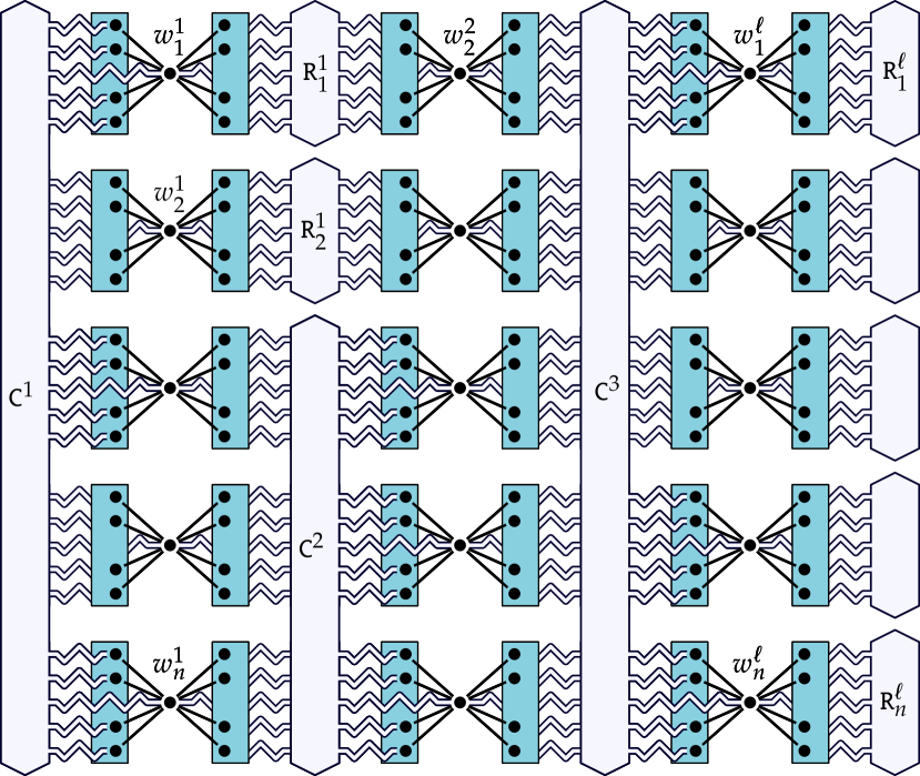
(a) The information vertices together with the managers and the consistency relations $\mathtt{R}_{i}^{j}$.

(b) The information vertices together with the managers and the constraint relations $\mathtt{C}^{j}$.

Figure 2: A depiction of the construction from the lower bound where ${\mathrm{m}}=5$, $n=5$, and $\ell=3$.

Consider a $q$-CSP-${\mathrm{m}}$ instance $I$ with $n$ variables and $\ell$ constraints. To achieve a low treewidth (or actually pathwidth), we construct a graph with $n\cdot\ell$ vertices, which we refer to as information vertices, that are arranged as an $n$ times $\ell$ grid. Each row of the grid corresponds to one variable and each column corresponds to one constraint. We refer to the information vertex from row $i$ and column $j$ as $w_{i}^{j}$. Note that every variable can take ${\mathrm{m}}$ different values. We encode these values by the states of the information vertices in the graph. As every vertex can have at least ${\mathrm{m}}$ states (in the finished the construction), we can assign a specific state to each possible variable value.

In order to provide sufficiently many neighbors to these information vertices, we introduce the concept of managers. A manager consists in this specific instance of $2n$ block, $n$ left blocks and $n$ right blocks, which can provide up to ${\mathrm{m}}-1$ neighbors to a vertex. We arrange these blocks as follows where we repeat this for each column (i.e., constraint). To each information vertex we add one left block and one right block on the respective side with regard to the grid layout. Then we make the information vertices adjacent with these block by ${\mathrm{m}}-1$ edges to distinguished vertices of the respective block. This results in every information vertex having in total $2{\mathrm{m}}-2$ adjacent vertices from two blocks. Even if the state of a vertex is determined by the total number of selected neighbors it has, in our setting we refer to the state of an information vertex as the number of neighbors it gets from the left block. By this convention we directly get a correspondence between the variable assignment and the states of the information vertices.

Despite this correspondence, the current construction suffers from the following misconception. Recall that we introduced for each column a separate manager that is not connected to the other managers. Therefore, the states of the information vertices might vary for the different columns even if we consider a single fixed row. Phrased differently, for a single fixed row, the states of the information vertices in this row might not be identical. A naive way to fix this behavior would be to add a single big relation to each row that observes all relevant vertices and enforces that the state is equal for all columns. However, this would result in a large treewidth which is not allowed. Instead, we add a small consistency relation $R_{i}^{j}$ between every two consecutive columns $j$ and $j+1$ for each row $i$.

Assume that we want to ensure the consistency between the information vertices $w_{i}^{j}$ and $w_{i}^{j+1}$. We define a relation which observes the right block of $w_{i}^{j}$ and the left block of $w_{i}^{j+1}$. This relation ensures at first that both vertices are unselected. Consider a setting where $w_{i}^{j}$ gets $b_{1}$ neighbors from its right block, and $w_{i}^{j+1}$ gets $b_{2}$ neighbors from its left block. Then the relation ensures that $b_{2}$ complements $b_{1}$ in the sense that $b_{2}$ is the smallest number such that $b_{1}+b_{2}=\min\rho\mod{\mathrm{m}}$. This especially implies that $b_{2}=\min\rho-b_{1}\mod{\mathrm{m}}$.

To establish that an assignment to the variables is consistently encoded in all columns, it remains to analyze the influence of the information vertices on the states of two neighboring columns. Assume that a selected information vertex $w_{i}^{j}$ receives $b_{0}$ neighbors from its left block of the manager and receives $b_{1}$ neighbors from the right block of the manager. Because we are considering a solution, vertex $w_{i}^{j}$ must have a valid number of neighbors. As the vertex $w_{i}^{j}$ has only neighbors in the two blocks, the solution must satisfy $b_{0}+b_{1}\in\rho$. Since $\rho$ is periodic with period $\rho$, we get $b_{0}+b_{1}=\min\rho\mod{\mathrm{m}}$ which implies that $b_{1}=\min\rho-b_{0}\mod{\mathrm{m}}$. When combining this with the observation from the previous paragraph where we consider two different information vertices, we get $b_{2}=\min\rho-(\min\rho-b_{0}\mod{\mathrm{m}})\mod{\mathrm{m}}$ and hence, $b_{2}=b_{0}\mod{\mathrm{m}}$ which implies that all information vertices of one row have the same status.

As a last step it remains to encode the constraints of the CSP instance. For each constraint $C_{j}$ we add one constraint relation $\mathtt{C}^{j}$ which observes the information vertices of the variables appearing in the constraint plus the neighbors of these vertices in the left block of the manager (they are needed to infer the state of the information vertices). The relation $\mathtt{C}^{j}$ then accepts a selection of vertices if it corresponds to a satisfying assignment.

This concludes the idea behind the lower bound for the intermediate problem $(\sigma,\rho)\mathchar 45\relax$DomSet${}^{\text{Rel}}$. To transform this bound into a bound for $(\sigma,\rho)\mathchar 45\relax$DomSet, we need to remove the relations and replace them by appropriate gadgets.

Step 2: Realizing the Relations.

Formally, the second step consists of proving the reduction from $(\sigma,\rho)\mathchar 45\relax$DomSet${}^{\text{Rel}}$ to $(\sigma,\rho)\mathchar 45\relax$DomSet. For this we replace each relation of the graph by a suitable gadget that precisely mimics the behavior of the original relation, that is, the gadget accepts a selection of vertices if and only if the original relation also accepted this selection. This especially means that the realization of the gadget is not allowed to add any selected neighbors to a vertex from the scope as this might have an effect on the existence of a solution (in the positive but also in the negative). See Definition 6.2 for a formal definition of a realization.

Curticapean and Marx [CM16] showed a method to realize arbitrary relations by just using two types of very specific relations. While proving the lower bounds for $(\sigma,\rho)\mathchar 45\relax$DomSet when $\sigma$ and $\rho$ are finite or cofinite, Focke et al. generalized this result further and showed that only one type of relations is sufficient in the case of $(\sigma,\rho)\mathchar 45\relax$DomSet [FMI⁺23c, Corollary 8.8]. More precisely, once we can realize a so-called $\mathtt{HW}_{=1}$ relation, then every relation can be realized. This $\mathtt{HW}_{=1}$ relation accepts if exactly one vertex from the scope of the relation is selected, that is, if the Hamming weight of the $\sigma$-vector is exactly one. We make this result even stronger by using an observation from [MSS21] which allows us to realize $\mathtt{HW}_{=1}$ for any arity based on realizations of $\mathtt{HW}_{=1}$ with arity one, two or three.

In order to realize these relations, we first realize an auxiliary relation. For some set $\tau$, the relation $\mathtt{HW}_{\in\tau}$ accepts, if and only if the number of selected vertices from the scope of the relation, i.e., the Hamming weight of the $\sigma$-vector, is contained in $\tau$. Once we set $\tau-k=\{t-k\mid t\in\tau\}$ to simplify notation, our main results for realizing relations reads as follows.

lemmarelationsHWOne Let $\sigma$ and $\rho$ be two difficult periodic sets with the same period ${\mathrm{m}}$. Then, the relation $\mathtt{HW}_{\in\rho-\min\rho+1}$ can be realized. Indeed, when assuming that ${\mathrm{m}}\geq 3$, then $\min\rho+1,\min\rho+2\notin\rho$. Restricting this gadget to arity at most $3$, directly realizes $\mathtt{HW}_{=1}$.

When we assume that the sets $\sigma$ and $\rho$ have period ${\mathrm{m}}=2$, then this gadget only gives $\mathtt{HW}_{=1}^{(1)}$ and $\mathtt{HW}_{=1}^{(2)}$. Intuitively this also agrees with our intuition that having $3$ selected neighbors is equivalent to having only $1$ selected neighbor. Recall that in this case the decision version is solvable in polynomial time. For these cases we consider the minimization version instead and focus on the two cases that are not trivially solvable; for $\rho=\{x\in\mathbb{Z}_{\geq 0}\mid x\equiv_{2}1\}$, we consider $\sigma=\{x\in\mathbb{Z}_{\geq 0}\mid x\equiv_{2}1\}$ and $\sigma=\{x\in\mathbb{Z}_{\geq 0}\mid x\equiv_{2}0\}$. In both cases we complement our algorithmic result from Section 1 by providing a matching lower bound based on the known NP-hardness result of the problem. As these proofs did not keep pathwidth low, we carefully modify the reduction by Sutner [Sut88] to obtain the matching bound.

3 Preliminaries

In this section we introduce some notation and concepts which we use in the following proofs. As we are dealing with the same problem as the work in [FMI⁺23a], we reuse many of their concepts and notation so that our results blend in more seamlessly.

3.1 Basic Notation

We write $\mathbb{Z}_{\geq 0}=\{n\in{\mathbb{Z}}\mid n\geq 0\}$ to denote the set of non-negative integers. For integers $i$ and $j$, we write $\bm{[}\,i\,\bm{.\,.}\,j\,\bm{]}$ for the set $\{n\in{\mathbb{Z}}\mid i\leq n\leq j\}$.

When $\Sigma$ is some alphabet, we write $\Sigma^{n}$ for the set (or language) of all strings of length $n$ over $\Sigma$. For a string $s\in\Sigma^{n}$, we index the positions of $s$ by integers from $\bm{[}\,1\,\bm{.\,.}\,n\,\bm{]}$ such that $s=s\bm{[}\,1\,\bm{]}s\bm{[}\,2\,\bm{]}\cdots s\bm{[}\,n\,\bm{]}$. For a set of positions $P\subseteq\bm{[}\,1\,\bm{.\,.}\,n\,\bm{]}$, we write $s\bm{[}\,P\,\bm{]}\coloneqq\bigcirc_{p\in P}\,s\bm{[}\,p\,\bm{]}$ for the string of length $|P|$ that contains only the symbols of $s$ whose indices are in $P$. We extend these notations in the standard way to vectors.

We use the notation $\Sigma^{X}$ for a finite set $X$ (for instance, a set of vertices of a graph), to emphasize that we index strings from $\Sigma^{\lvert X\rvert}$ by elements from $X$.

3.2 Graphs

Unless mentioned otherwise, a graph is a pair $G=(V(G),E(G))$ with a finite vertex set $V(G)$ and a finite edge set $E(G)\subseteq\binom{V(G)}{2}$. When the graph is clear from the context, we also just write $G=(V,E)$. In this paper, all considered graphs are undirected and simple, that is, they have no loops or multiple edges, unless explicitly stated otherwise. For an edge $\{u,v\}\in E(G)$, we also write $uv$ to simplify notation.

For a vertex $v\in V(G)$, we denote by $N_{G}(v)$ the (open) neighborhood of $v$ that is, $N_{G}(v)\coloneqq\{w\in V(G)\mid vw\in E(G)\}$. We denote the closed neighborhood of $v$ by $N_{G}\bm{[}\,v\,\bm{]}\coloneqq N_{G}(v)\cup\{v\}$. The degree of $v$ is the size of its open neighborhood, that is, $\deg_{G}(v)\coloneqq|N_{G}(v)|$. When $X\subseteq V(G)$ is a set of vertices, we define the closed neighborhood of $X$ as $N_{G}\bm{[}\,X\,\bm{]}\coloneqq\bigcup_{v\in X}N_{G}\bm{[}\,v\,\bm{]}$ and the open neighborhood of $X$ as $N_{G}(X)\coloneqq N_{G}\bm{[}\,X\,\bm{]}\setminus X$. We may drop the subscript $G$ in all settings if the graph is clear from the context.

For a vertex set $X\subseteq V(G)$, we denote by $G\bm{[}\,X\,\bm{]}$ the induced subgraph on the vertex set $X$. By $G-X$ we denote the induced subgraph on the complement of $X$, and formally define $G-X\coloneqq G\bm{[}\,V(G)\setminus X\,\bm{]}$.

3.3 Treewidth

Our algorithmic results are based on tree decompositions. For completeness, we restate the definition and the basic properties of such a decomposition. We refer the reader to [CFK⁺15, Chapter 7] for a more detailed introduction to the concept.

Consider a graph $G$. A tree decomposition of $G$ is a pair $(T,\beta)$ that consists of a rooted tree $T$ and a function $\beta\colon V(T)\to 2^{V(G)}$ such that

1. $\bigcup_{t\in V(T)}\beta(t)=V(G)$,

2. for every edge $vw\in E(G)$, there is some node $t\in V(T)$ such that $\{u,v\}\subseteq\beta(t)$, and

3. for every $v\in V(G)$, the set $\{t\in V(T)\mid v\in\beta(t)\}$ induces a connected subtree of $T$.

The width of a tree decomposition $(T,\beta)$ is defined as $\max_{t\in V(T)}|\beta(t)|-1$. The treewidth of a graph $G$, denoted by $\textup{{tw}}(G)$, is the minimum width of a tree decomposition of $G$.

In order to design algorithm based on tree decompositions, it is usually helpful to use nice tree decompositions. Let $(T,\beta)$ denote a tree decomposition and write $X_{t}\coloneqq\beta(t)$ for the bag of a node $t\in V(T)$. We say that $(T,\beta)$ is a nice tree decomposition, or nice for short, if the tree $T$ is a binary tree rooted at some node $r$ such that $X_{r}=\varnothing$ and every node $t\in V(T)$ of the decomposition has one of the following types:

Leaf Node:

Node $t$ has no children and an empty bag, that is, $t$ is a leaf of $T$ and $X_{t}=\varnothing$.

Introduce Node:

Node $t$ has exactly one child $t^{\prime}$ and $X_{t}=X_{t^{\prime}}\cup\{v\}$ for some $v\notin X_{t^{\prime}}$, we say that the vertex $v$ is introduced at $t$.

Forget Node:

Node $t$ has exactly one child $t^{\prime}$ and $X_{t}=X_{t^{\prime}}\setminus\{v\}$ for some $v\in X_{t^{\prime}}$, we say that the vertex $v$ is forgotten at $t$.

Join Node:

Node $t$ has exactly two children $t_{1},t_{2}$ and $X_{t}=X_{t_{1}}=X_{t_{2}}$.

In time $\mathcal{O}(\textup{{tw}}^{2}\cdot\max\{|V(G),V(T)|\})$, we can transform every given tree decomposition $(T,\beta)$ of width tw for a graph $G$ into a nice tree decomposition of size $\mathcal{O}(\textup{{tw}}\cdot V(T))$ of the same width (see, for example, [CFK⁺15, Lemma 7.4]).

The concepts path decomposition and pathwidth follow analogously by additionally requiring that the underlying tree $T$ is a path.

3.4 Partial Solutions and States

When formally describing the algorithm and designing the lower bounds, we frequently consider subgraphs (of the final graph) and argue about the intersection of solutions with this subgraph. In order to describe the interaction between the subgraph and the remaining graph, we use the notion of a graph with portals. These portals are then separating the subgraph from the remaining graph. For the algorithmic result the portals are the vertices of the bag, and for the lower bounds the portals are vertices in the scope of some relation.

Definition 3.1 (Graph with Portals; compare [FMI⁺23b, Section 3]).

A graph with portals $G$ is a pair $(G^{\prime},U)$, where $G^{\prime}$ is a graph and $U\subseteq V(G)$. If $U=\{u_{1},\dots,u_{k}\}$, then we also write $(G^{\prime},u_{1},\dots,u_{k})$ instead of $(G^{\prime},U)$.

If it is clear from the context, we also refer to a graph with portals simply as a graph.

With the formal notion of a graph with relations, we can now also define a partial solution. These partial solutions capture the intersection of a (hypothetical) solution with the vertices from a graph with portals.

Definition 3.2 (Partial Solution [FMI⁺23b, Definition 3.3]).

Fix a graph with portals $(G,U)$. A set $S\subseteq V(G)$ is a partial solution (with respect to $U$) if

1. for each $v\in S\setminus U$, we have $|N(v)\cap S|\in\sigma$, and

2. for each $v\in V(G)\setminus(S\cup U)$, we have $|N(v)\cap S|\in\rho$.

When designing the algorithm or when constructing the gadgets, we usually do not want to argue about every possible partial solution but identify those solutions that behave equivalently when considering their extension to the remaining graph. Formally, we associate with each partial solution for a graph with relations a state for each portal vertex. This state describes whether a vertex is selected or not and how many neighbors it gets from this partial solution.

In order to argue about these different states, we define different set of states.

Definition 3.3 (States).

For all $i\in\mathbb{Z}_{\geq 0}$, we define a $\sigma$-state $\sigma_{i}$ and a $\rho$-state $\rho_{i}$. We use ${\mathbb{S}}$ and ${\mathbb{R}}$ for the sets of all $\sigma$-states and all $\rho$-states. We denote by ${\mathbb{A}}\coloneqq{\mathbb{S}}\cup{\mathbb{R}}$ the set of all states.

When our sets $\sigma$ and $\rho$ are periodic with period ${\mathrm{m}}_{\sigma}$ and ${\mathrm{m}}_{\rho}$, respectively, we define

• ${\mathbb{S}}\coloneqq\{\sigma_{0},\dots,\sigma_{{\mathrm{m}}_{\sigma}-1}\}$ to be the set of $\sigma$ states,

• ${\mathbb{R}}\coloneqq\{\rho_{0},\dots,\rho_{{\mathrm{m}}_{\rho}-1}\}$ to be the set of $\rho$ states, and

• ${\mathbb{A}}\coloneqq{\mathbb{S}}\cup{\mathbb{R}}$ the set of all states.

Even if the sets are periodic, these states capture all relevant states. For example, consider the case in which $\sigma$ and $\rho$ are the sets of all even integers. Then, it does not matter whether a vertex has $2$ or $42$ selected neighbors; both states show exactly the same behavior with regard to adding more neighbors to the respective vertex.

With the above notation about strings and vectors in mind, we usually define strings over the alphabets ${\mathbb{S}}$, ${\mathbb{R}}$, or ${\mathbb{A}}$. In this case we usually index the positions of such strings by a vertex of a bag or by a vertex of the scope of a relation. Then, we can relate the partial solutions and the states of the portal vertices via compatible strings.

Definition 3.4 (Compatible Strings, extension of [FMI⁺23b, Definition 3.4]).

Fix a graph with portals $(G,U)$. A string $x\in{\mathbb{A}}^{U}$ is compatible with $(G,U)$ if there is a partial solution $S_{x}\subseteq V(G)$ such that

1. for each $v\in U\cap S_{x}$, we have $x\bm{[}\,v\,\bm{]}=\sigma_{s}$, where

   • $s=|N(v)\cap S_{x}|\bmod{\mathrm{m}}_{\sigma}$ when $\sigma$ is periodic with period ${\mathrm{m}}_{\sigma}$,

   • $s=|N(v)\cap S_{x}|$ otherwise,

2. for each $v\in U\setminus S_{x}$, we have $x\bm{[}\,v\,\bm{]}=\rho_{r}$, where

   • $r=|N(v)\cap S_{x}|\bmod{\mathrm{m}}_{\rho}$ when $\rho$ is periodic with period ${\mathrm{m}}_{\rho}$,

   • $r=|N(v)\cap S_{x}|$ otherwise.

We also refer to the vertices in $S_{x}$ as being selected and say that $S_{x}$ is a (partial) solution, selection, or witness that witnesses $x$.

Then, given a graph with portals $(G,U)$, the set of all strings compatible with this graph is of utmost importance, we call this set the realized language of the graph.

Definition 3.5 (Realized Language and $L$-provider [FMI⁺23c, Definition 3.9]).

For a graph with portals $(G,U)$, we define its realized language as

$$L(G,U)\coloneqq\{x\in{\mathbb{A}}^{U}\mid x\text{ is compatible with }(G,U)\}.$$

For a language $L\subseteq{\mathbb{A}}^{U}$, we say that $(G,U)$ is an $L$-realizer if $L=L(G,U)$.

For a language $L\subseteq{\mathbb{A}}^{U}$, we say that $(G,U)$ is an $L$-provider if $L\subseteq L(G,U)$.

4 Upper Bound

In this section we prove the algorithmic result for $(\sigma,\rho)\mathchar 45\relax$DomSet when the sets $\sigma$ and $\rho$ are periodic with the same period ${\mathrm{m}}\geq 2$ when parameterizing by treewidth. This closely matches our lower bound from Section 1. Note that when ${\mathrm{m}}=1$, the sets contain all numbers and thus, the problem is trivially solvable (any subset of the vertices is a solution). Formally, we prove Section 1.

*

We use the known results from [FMI⁺23b] as a starting point and extend these results to the case when we have periodic sets. This requires us to adjust several concepts and introduce new results where the results form the finite case are not applicable. However, as we are dealing with periodic sets only which furthermore have the same period, this allows a simpler presentation of the results.

As already mentioned earlier, the final algorithm is based on dynamic programming on the tree decomposition of the given graph. In order to obtain an upper bound, which matches the stated lower bound from Section 1, there are three main problems that we have to overcome:

• We need to prove a tight bound on the number of different types of partial solutions for a certain graph. We store these states for each node of the tree decomposition in order to correctly solve the problem.

• Since the running time of the join operation (from the next step) depends on the size of the space, we additionally need to compress the space of state-vectors. A simple bound on the number of states is actually not sufficient.

• To compute the join nodes efficiently without dominating the running time of the problem, we need to employ a fast convolution technique to compute the join nodes.

We handle these problems in the stated order and start in Section 4.1 by bounding the number of different types of partial solutions for a graph with portals. Then in Section 4.2 we formally introduce the concept of compressions, which we then need in Section 4.3 to state the procedure which computes the join nodes efficiently. As a last step we state the final algorithm in Section 4.4.

Before moving to the first step, we first formally define how a state vector can be decomposed into a $\sigma$-vector and weight-vector. The definition closely mirrors [FMI⁺23b, Definition 4.2] adjusted to our setting.

Definition 4.1 (Decomposing States).

For a string $x\in{\mathbb{A}}^{n}$ representing a state-vector, we define

• the $\sigma$-vector of $x$ as $\overrightarrow{\sigma}(x)\in\{0,1\}^{n}$ with

  $$\overrightarrow{\sigma}(x)\bm{[}\,i\,\bm{]}\coloneqq\left\{\begin{array}[]{@{\;}c@{\quad}l@{}}1,&\text{if }x\bm{[}\,i\,\bm{]}\in{\mathbb{S}},\\ 0,&\text{if }x\bm{[}\,i\,\bm{]}\in{\mathbb{R}},\end{array}\right.$$

• and the weight-vector of $x$ as $\overrightarrow{\mathrm{w}}(x)\in{\mathbb{Z}}_{\geq 0}^{n}$ with

  $$\overrightarrow{\mathrm{w}}(x)\bm{[}\,i\,\bm{]}\coloneqq c,\quad\text{where }x\bm{[}\,i\,\bm{]}\in\{\sigma_{c},\rho_{c}\}.$$

We extend this notion to languages $L\subseteq{\mathbb{A}}^{n}$ in the natural way. Formally, we write $\overrightarrow{\sigma}(L)\coloneqq\{\overrightarrow{\sigma}(x)\mid x\in L\}$ for the set of all $\sigma$-vectors of $L$, and we write $\overrightarrow{\mathrm{w}}(L)\coloneqq\{\overrightarrow{\mathrm{w}}(x)\mid x\in L\}$ for the set of all weight-vectors of $L$.

4.1 Bounding the Size of A Single Language

We start our theoretical considerations by considering the realized language of a graph with portals. The goal of this section is to show that for any graph with portals $(G,U)$, the size of the realized language is small.

To formally state the result, we first introduce the concept of a sparse language.

Definition 4.2 (Sparse Language; compare [FMI⁺23b, Page 16]).

Let $\sigma$ and $\rho$ denote two periodic sets with the same period ${\mathrm{m}}\geq 2$. We say that a language $L\subseteq\mathbb{A}^{n}$ is sparse if for all $x,y\in L$ the following holds: $\overrightarrow{\sigma}(x)\cdot\overrightarrow{\mathrm{w}}(y)\equiv_{\mathrm{m}}\overrightarrow{\sigma}(y)\cdot\overrightarrow{\mathrm{w}}(x)$.

Even though the definition of a sparse language does not say anything about the size of the realized language, we show that this is the correct notation by proving the following result. For the case when both sets are finite, the result is covered by [FMI⁺23b, Theorem 4.4] which we extend to periodic sets.

lemmathmUpperBoundOnLanguage Let $\sigma$ and $\rho$ denote two periodic sets with the same period ${\mathrm{m}}\geq 2$. Every sparse language $L\subseteq\mathbb{A}^{n}$ satisfies $|L|\leq{\mathrm{m}}^{n}$.

Instead of later directly proving that a language is sparse, we usually use the following sufficient condition, which intuitively reads as, “if the number of selected non-portal vertices for every pair of solutions is equal modulo ${\mathrm{m}}$, then the language is sparse”.

Proof 4.3.

We observe that the proof of [FMI⁺23b, Lemma 4.3] does not use the finiteness of $\sigma$ or $\rho$. Although this means that the proof works for our setting as well, we provide it here for completeness. Note that this proof does not assume that the sets $\sigma$ and $\rho$ are periodic. Therefore, we denote by $s\in\sigma$ and $r\in\rho$ two elements of the sets to argue about the remainder when dividing by ${\mathrm{m}}$.

We prove the claim by counting edges between $S_{x}$ to $S_{y}$ in two different ways. First we count the edges as going from $S_{x}$ to $S_{y}$. Let $E(X\to Y)=\{(u,v)\in E(G)\mid u\in X,v\in Y\}$ denote the set of edges from $X$ to $Y$.

We partition the vertices of $S_{x}$ into (1) vertices that are neither in $U$ nor $S_{y}$, (2) the vertices that are in $S_{y}$, and (3) the vertices that are in $U$. Every vertex in $S_{x}$ that is neither in $S_{y}$ nor in $U$, is unselected in $S_{y}$ and thus, the number of neighbors it has in $S_{y}$ must be in $\rho$ because $S_{y}$ is a partial solution. Especially, this number must be congruent $r\bmod{\mathrm{m}}$ because $\rho$ is ${\mathrm{m}}$-structured. If a vertex is in $S_{x}$ and in $S_{y}$ but not in $U$, then the number of neighbors it has in $S_{y}$ must be congruent $s\bmod{\mathrm{m}}$ for the analogous reason. It remains to elaborate on the edges leaving from vertices in $U$. Such a vertex only contributes to the count if it is selected in $S_{x}$, i.e., if the $\sigma$-vector is $1$ at the considered position. The actual number of neighbors such a vertex receives in $S_{y}$ is determined by the entry of the weight-vector for $S_{y}$ at the corresponding coordinate. Combining these observations yields,

$$|{E(S_{x}\to S_{y})}|\equiv_{\mathrm{m}}\leavevmode\nobreak\ r\cdot|S_{x}\setminus(S_{y}\cup U)|$$

$$+s\cdot|(S_{x}\cap S_{y})\setminus U|$$

$$+\overrightarrow{\sigma}(x)\cdot\overrightarrow{\mathrm{w}}(y)$$

$$\equiv_{\mathrm{m}}\leavevmode\nobreak\ r\cdot(|S_{x}\setminus U|-|S_{x}\cap S_{y}|+|S_{x}\cap S_{y}\cap U|)$$

$$+s\cdot|(S_{x}\cap S_{y})\setminus U|$$

$$+\overrightarrow{\sigma}(x)\cdot\overrightarrow{\mathrm{w}}(y).$$

Flipping the roles of $S_{x}$ and $S_{y}$ gives

$$|{E(S_{y}\to S_{x})}|\equiv_{\mathrm{m}} \leavevmode\nobreak\ r\cdot(|S_{y}\setminus U|-|S_{x}\cap S_{y}|+|S_{x}\cap S_{y}\cap U|)$$

$$+s\cdot|(S_{y}\cap S_{x})\setminus U$$

$$+\overrightarrow{\sigma}(y)\cdot\overrightarrow{\mathrm{w}}(x).$$

Observe that we have $|E(S_{x}\to S_{y})|=|E(S_{y}\to S_{x})|$ since both sets count every edge from solution $S_{x}$ to solution $S_{y}$ exactly once and the edges are undirected. Using these properties and the assumption that $|S_{x}\setminus U|\equiv_{\mathrm{m}}|S_{y}\setminus U|$, we get from the combination of the above equations that

$$\overrightarrow{\sigma}(x)\cdot\overrightarrow{\mathrm{w}}(y)\equiv_{\mathrm{m}}\overrightarrow{\sigma}(y)\cdot\overrightarrow{\mathrm{w}}(x).$$

Toward showing that sparse languages are indeed of small size, we establish one auxiliary property that immediately follows from the definition of a sparse language.

Lemma 4.4 (Compare [FMI⁺23b, Lemma 4.6]).

Let $\sigma$ and $\rho$ denote two periodic sets with period ${\mathrm{m}}\geq 2$. Let $L\subseteq\mathbb{A}^{n}$ be a sparse language. For any three strings $x,y,z\in L$ with $\overrightarrow{\sigma}(x)=\overrightarrow{\sigma}(y)$, we have

$$\left(\overrightarrow{\mathrm{w}}(x)-\overrightarrow{\mathrm{w}}(y)\right)\cdot\overrightarrow{\sigma}(z)\equiv_{\mathrm{m}}0.$$

Proof 4.5.

We reproduce the proof of the original result in [FMI⁺23b]. Let $L$ be a sparse language, and consider state-vectors $x,y,z\in L$ with $\overrightarrow{\sigma}(x)=\overrightarrow{\sigma}(y)$. Because $L$ is sparse we know that

$$\overrightarrow{\sigma}(z)\cdot\overrightarrow{\mathrm{w}}(x)\equiv_{\mathrm{m}}\overrightarrow{\sigma}(x)\cdot\overrightarrow{\mathrm{w}}(z)$$

and by $\overrightarrow{\sigma}(x)=\overrightarrow{\sigma}(y)$, this gives

$$\overrightarrow{\sigma}(z)\cdot\overrightarrow{\mathrm{w}}(x)\equiv_{\mathrm{m}}\overrightarrow{\sigma}(y)\cdot\overrightarrow{\mathrm{w}}(z).$$

When using the properties of sparsity for $y$ and $z$ we have

$$\overrightarrow{\sigma}(y)\cdot\overrightarrow{\mathrm{w}}(z)\equiv_{\mathrm{m}}\overrightarrow{\sigma}(z)\cdot\overrightarrow{\mathrm{w}}(y).$$

Combining the last two results, yields

$$\overrightarrow{\sigma}(z)\cdot\overrightarrow{\mathrm{w}}(x)\equiv_{\mathrm{m}}\overrightarrow{\sigma}(z)\cdot\overrightarrow{\mathrm{w}}(y)$$

and rearranging this equivalence concludes the proof.

Intuitively, the condition of the previous lemma significantly restricts the number of possible weight-vectors of two different strings with the same $\sigma$-vector. This restriction is the reason why sparse languages turn out to be of small size. To formalize how restrictive this condition is exactly, we introduce the notion of $\sigma$-defining sets. Such a set depends only on a set of binary vectors, for example, the $\sigma$-vectors of a sparse language, and provides us $\sigma$-vectors of the language that are very similar.

Definition 4.6 ($\sigma$-defining set; compare [FMI⁺23b, Definition 4.7]).

A set $S\subseteq\bm{[}\,1\,\bm{.\,.}\,n\,\bm{]}$ is $\sigma$-defining for $X\subseteq\{0,1\}^{n}$ if $S$ is an inclusion-minimal set of positions that uniquely characterize the vectors of $X$, that is, for all $u,v\in X$, we have

$$u\bm{[}\,S\,\bm{]}=v\bm{[}\,S\,\bm{]}\quad\text{implies}\quad u=v.$$

For a $\sigma$-defining set $S$ of a set $X\subseteq\{0,1\}^{n}$, we additionally define the complement of $S$ as $\overline{S}\coloneqq\bm{[}\,1\,\bm{.\,.}\,n\,\bm{]}\setminus S$.

The name of the $\sigma$-defining sets comes from the fact that we usually use a set of $\sigma$-vectors for the set $X$.

Fact 1 ([FMI⁺23b, Remark 4.8]).

As a $\sigma$-defining $S$ of a set $X\subseteq\{0,1\}^{n}$ is (inclusion-wise) minimal, observe that, for each position $i\in S$, there are pairs of witness vectors $w_{1,i},w_{0,i},\in X$ that differ (on $S$) only at position $i$, with $w_{1,i}\bm{[}\,i\,\bm{]}=1$, that is,

• $w_{1,i}\bm{[}\,S\setminus i\,\bm{]}=w_{0,i}\bm{[}\,S\setminus i\,\bm{]}$,

• $w_{1,i}\bm{[}\,i\,\bm{]}=1$, and

• $w_{0,i}\bm{[}\,i\,\bm{]}=0$.

We write ${\mathcal{W}}_{S}\coloneqq\{w_{1,i},w_{0,i}\mid i\in S\}$ for a set of witness vectors of $X$.

Before we start using these $\sigma$-defining sets, we first show how to compute them efficiently along with the witness vectors. The result is similar to [FMI⁺23b, Lemma 4.27]. However, we improve the running time of the algorithm by using a more efficient approach to process the data.

Lemma 4.7.

Given a set $X\subseteq\{0,1\}^{n}$, we can compute a $\sigma$-defining set $S$ for $X$, as well as a set of witness vectors ${\mathcal{W}}_{S}$ for $S$, in time $\mathcal{O}(|X|\cdot n^{3})$.

Proof 4.8.

Our algorithm maintains a set $S\subseteq\bm{[}\,1\,\bm{.\,.}\,n\,\bm{]}$ as the candidate for the $\sigma$-defining set for $X$ and iteratively checks if a position can be removed from $S$ or whether it is part of the $\sigma$-defining set. Formally, the algorithm is as follows.

• Initialize the candidate set as $S=\bm{[}\,1\,\bm{.\,.}\,n\,\bm{]}$.

• For all $i$ from $1$ to $n$, repeat the following steps:

  • Initialize an empty map data structure, for example, a map based on binary trees.

  • Iterate over all $v\in X$:

    If there is no entry with key $v\bm{[}\,S\setminus\{i\}\,\bm{]}$ in the map, we add the value $v$ with the key $v\bm{[}\,S\setminus\{i\}\,\bm{]}$ to the map.

    If there is already an entry with key $v\bm{[}\,S\setminus\{i\}\,\bm{]}$ and value $v^{\prime}$ in the map. Then, define the two witness-vectors $w_{0,i}$ and $w_{1,i}$ for position $i$ as $v$ and $v^{\prime}$ (depending on $i$th bit of $v$ and $v^{\prime}$), and continue with the (outer) for-loop.

  • Remove position $i$ from $S$ and continue with the next iteration of the for-loop.

• Output $S$ as the $\sigma$-defining set and ${\mathcal{W}}_{S}=\{w_{0,i},w_{1,i}\mid i\in S\}$ as the set of witness vectors.

From the description of the algorithm, each operation of the for-loop takes time $\mathcal{O}(|X|\cdot\log(|X|)\cdot n)=\mathcal{O}(|X|\cdot n^{2})$. It follows that $S$ can be computed in time $\mathcal{O}(|X|\cdot n^{3})$.

In order to prove the correctness, we denote by $S_{i}$ the set $S$ after the $i$th iteration of the for-loop and denote by $S_{0}=\bm{[}\,1\,\bm{.\,.}\,n\,\bm{]}$ the initial set. Hence, the algorithm returns $S_{n}$. We prove by induction that, for all $i\in\bm{[}\,0\,\bm{.\,.}\,n\,\bm{]}$, if there are $u,v\in X$ with $x\bm{[}\,S_{i}\,\bm{]}=y\bm{[}\,S_{i}\,\bm{]}$, then $u=v$. This is clearly true for $i=0$ by the choice of $S_{0}$. For the induction step, assume that the claim holds for an arbitrary but fixed $i-1\in\bm{[}\,0\,\bm{.\,.}\,n-1\,\bm{]}$ where $S_{i}\neq S_{i-1}$ as otherwise the claim follows by the induction hypothesis. By the design of the algorithm, we know that $S_{i}=S_{i-1}\setminus\{i\}$. Moreover, as $i$ was removed from $S_{i-1}$, there are no two vectors $u,v\in X$ such that $u\bm{[}\,S_{i-1}\setminus\{i\}\,\bm{]}=v\bm{[}\,S_{i-1}\setminus\{i\}\,\bm{]}$. This directly implies that, for all $u,v\in X$, the vectors $u$ and $v$ differ on $S_{i}\setminus\{i\}$ and thus, are not equal.

It remains to prove that $S_{n}$ is minimal. Assume otherwise and let $i\in S_{n}$ be some index such that, for all $u,v\in X$, we still have $u=v$ whenever

$$u\bm{[}\,S_{n}\setminus\{i\}\,\bm{]}=v\bm{[}\,S_{n}\setminus\{i\}\,\bm{]}.$$ (1)

As the algorithm did not remove $i$ from $S_{i-1}$, we know that there must be at least two vectors $\hat{u},\hat{v}\in X$ with $\hat{u}\neq\hat{v}$ such that

$$\hat{u}\bm{[}\,S_{i-1}\setminus\{i\}\,\bm{]}=\hat{v}\bm{[}\,S_{i-1}\setminus\{i\}\,\bm{]}.$$ (2)

Since the algorithm satisfies $S_{0}\supseteq S_{1}\supseteq\dots\supseteq S_{n}$, we especially have $S_{n}\subseteq S_{i-1}$ and thus, whenever Equation 2 holds, then also Equation 1 holds which implies that $\hat{u}=\hat{v}$. As this contradicts $\hat{u}\neq\hat{v}$, we know that $S_{n}$ is a $\sigma$-defining set.

To see that the vectors in ${\mathcal{W}}_{S}$ are indeed witness-vectors, recall that the algorithm guarantees that the distinct vectors $w_{0,i}$ and $w_{1,i}$ satisfy $w_{0,i}\bm{[}\,S_{i-1}\setminus\{i\}\,\bm{]}=w_{1,i}\bm{[}\,S_{i-1}\setminus\{i\}\,\bm{]}$. Moreover, the inductive proof above shows that $w_{0,i}\bm{[}\,S_{i-1}\,\bm{]}\not=w_{1,i}\bm{[}\,S_{i-1}\,\bm{]}$, and hence, $w_{0,i}\bm{[}\,i\,\bm{]}\not=w_{1,i}\bm{[}\,i\,\bm{]}$. Finally, since $S_{i-1}\subseteq S_{n}$, the vectors agree on $S_{n}\setminus\{i\}$ which concludes the proof.

Now we can concretize how Lemma 4.4 restricts the possible weight-vectors of two strings with the same $\sigma$-vector. Intuitively, what the $\sigma$-defining set is for the vector $\overrightarrow{\sigma}(v)$, this is the set $\overline{S}$ for the weight-vector. We could say that $\overline{S}$ is a weight-defining set. This extends [FMI⁺23b, Lemma 4.9] to the periodic case.

Proof 4.9.

We adjust the proof in [FMI⁺23b] to our setting. Let $L$ be a sparse language with $S$ as a $\sigma$-defining set for $\overrightarrow{\sigma}(L)$. Furthermore, consider two state-vectors $x$ and $y$ of $L$ with the same $\sigma$-vector, i.e., $\overrightarrow{\sigma}(x)=\overrightarrow{\sigma}(y)$, such that $\overrightarrow{\mathrm{w}}(x)\bm{[}\,\overline{S}\,\bm{]}=\overrightarrow{\mathrm{w}}(y)\bm{[}\,\overline{S}\,\bm{]}$.

Fix a position $\ell\in S$. We have binary witness vectors $w_{1,\ell}$ and $w_{0,\ell}$, that agree on all positions of $S$ except for position $\ell$ and satisfy $w_{1,\ell}\bm{[}\,\ell\,\bm{]}=1$.

Using Lemma 4.4 twice we obtain

$$(\overrightarrow{\mathrm{w}}(x)-\overrightarrow{\mathrm{w}}(y))\cdot(w_{1,\ell}-w_{0,\ell})\equiv_{\mathrm{m}}0.$$

By the assumption about $x$ and $y$, their weight-vectors agree on all positions in $\overline{S}$. But since $w_{1,\ell}$ and $w_{0,\ell}$ are identical on all positions of $S$ except for position $\ell$, this means that

$$0\equiv_{\mathrm{m}}\leavevmode\nobreak\ (\overrightarrow{\mathrm{w}}(x)-\overrightarrow{\mathrm{w}}(y))\cdot(w_{1,\ell}-w_{0,\ell})$$

$$\equiv_{\mathrm{m}}\leavevmode\nobreak\ \overrightarrow{\mathrm{w}}(x)\bm{[}\,\ell\,\bm{]}-\overrightarrow{\mathrm{w}}(y)\bm{[}\,\ell\,\bm{]}.$$

Since all values of the weight-vector are less than ${\mathrm{m}}$, the consequence $\overrightarrow{\mathrm{w}}(x)\bm{[}\,\ell\,\bm{]}=\overrightarrow{\mathrm{w}}(y)\bm{[}\,\ell\,\bm{]}$ concludes the proof.

The previous result from Section 2.1 gives rise to a strategy for counting all the strings of a sparse language. Namely, we can fix a $\sigma$-vector and count the number of strings with this fixed vector, which is the same as the number of weight-vectors of strings with this fixed $\sigma$-vector. When counting the weight-vectors, we can now use the property we have just seen to show that not every weight-vector can actually occur.

Proof 4.10.

Let $L\subseteq\mathbb{A}^{n}$ be a sparse language. Compute a $\sigma$-defining set $S$ for $\overrightarrow{\sigma}(L)$.

The size of $\overrightarrow{\sigma}(L)$ is bounded by $2^{|S|}$ per definition. Fix an arbitrary $\sigma$-vector $\vec{s}$ of $\overrightarrow{\sigma}(L)$. We now count the number of possible weight-vectors with $\sigma$-vector $\vec{s}$. By Section 2.1, the positions $\overline{S}$ of the weight-vector uniquely determine the positions $S$ of the weight vector. Hence, we obtain a bound on the size of the language of

$$|L|\leq 2^{|S|}\cdot{\mathrm{m}}^{|\overline{S}|}\leq{\mathrm{m}}^{n}.$$

4.2 Compressing Weight-Vectors

In the previous section we have seen that the size of a language cannot be too large. However, even though this already provides a bound on the size of these languages, the space where these languages come from is still large. That is, even when considering a sparse language $L\subseteq{\mathbb{A}}^{n}$, we would have to consider all states in ${\mathbb{A}}^{n}$ when doing convolutions as we do not know which vectors might actually appear in the solution. The goal of this section is to provide the concept of compression where we do not only compress the vectors of a language but actually compress the space where these vectors are from.

In previous sections we have seen that certain positions of the weight-vectors actually uniquely determine the remaining positions. Hence, a natural idea for the compression of strings is to store the values at important positions only, while ensuring that the values at the other positions can be reconstructed.

We first introduce the notion of the remainder. Intuitively, the remainder can be used to reconstruct the values of the weight-vector which have been compressed.

Definition 4.11 (Compare [FMI⁺23b, Definition 4.21]).

Let $\sigma$ and $\rho$ denote two periodic sets with period ${\mathrm{m}}\geq 2$. Let $L\subseteq{\mathbb{A}}^{n}$ denote a (non-empty) sparse language. Consider a set $X$ with $X\subseteq\overrightarrow{\sigma}(L)$ and $X\not=\varnothing$, and let $S$ denote a $\sigma$-defining set for $X$ with a corresponding set of witness vectors ${\mathcal{W}}_{S}\subseteq\overrightarrow{\sigma}(L)$. For two vectors $u,o\in\bm{[}\,0\,\bm{.\,.}\,{\mathrm{m}}-1\,\bm{]}^{n}$ and a position $\ell\in S$, we define the remainder $\mathrm{rem}_{{\mathcal{W}}_{S}}(u,o)$ at position $\ell$ as

$$\mathrm{rem}_{{\mathcal{W}}_{S}}(u,o)\bm{[}\,\ell\,\bm{]}\coloneqq\sum_{i\in\overline{S}}\big{(}u\bm{[}\,i\,\bm{]}-o\bm{[}\,i\,\bm{]}\big{)}\cdot\big{(}w_{1,\ell}\bm{[}\,i\,\bm{]}-w_{0,\ell}\bm{[}\,i\,\bm{]}\big{)}.$$

As a next step we show that this remainder is chosen precisely in such a way that we can easily reconstruct the values of the weight-vector on positions $S$.

Lemma 4.12 (Compare [FMI⁺23b, Remark 4.22]).

Let $\sigma$ and $\rho$ denote two periodic sets with the same period ${\mathrm{m}}$. Let $L\subseteq{\mathbb{A}}^{n}$ denote a (non-empty) sparse language. Consider a set $X$ with $X\subseteq\overrightarrow{\sigma}(L)$ and $X\not=\varnothing$, and let $S$ denote a $\sigma$-defining set for $X$ with a corresponding set of witness vectors ${\mathcal{W}}_{S}\subseteq\overrightarrow{\sigma}(L)$. Consider arbitrary weight-vectors $u$ and $o$ of two strings from $L$ with a common $\sigma$-vector. Then,

$$u\bm{[}\,\ell\,\bm{]}\equiv_{\mathrm{m}}o\bm{[}\,\ell\,\bm{]}-\mathrm{rem}_{\mathcal{W}_{S}}(u,o)\bm{[}\,\ell\,\bm{]}$$

holds for all $\ell\in S$.

Proof 4.13.

We follow the sketch provided in [FMI⁺23b]. Let $u$ and $o$ be two weight-vectors of two strings of $L$ that share a common $\sigma$-vector. By the definition of the $\sigma$-defining set, there are, for all $\ell\in S$, two associated witness vectors $w_{0,\ell},w_{1,\ell}\in\overrightarrow{\sigma}(L)$. Hence, there exist two strings $x,y\in L$ such that $\overrightarrow{\sigma}(x)=w_{0,\ell}$ and $\overrightarrow{\sigma}(y)=w_{1,\ell}$. From Lemma 4.4 we obtain

$$(u-o)\cdot w_{1,\ell}\equiv_{\mathrm{m}}0\qquad\text{and similarly}\qquad(u-o)\cdot w_{0,\ell}\equiv_{\mathrm{m}}0.$$

Recall that $w_{0,\ell}$ and $w_{1,\ell}$ agree on all positions of $S$ except for position $\ell$, which implies that $w_{1,\ell}\bm{[}\,i\,\bm{]}-w_{0,\ell}\bm{[}\,i\,\bm{]}=0$ for all $i\in S\setminus\{\ell\}$. Combining these observations we get

$$u\bm{[}\,\ell\,\bm{]}-o\bm{[}\,\ell\,\bm{]}+\mathrm{rem}_{\mathcal{W}_{S}}(u,o)\bm{[}\,\ell\,\bm{]} =u\bm{[}\,\ell\,\bm{]}-o\bm{[}\,\ell\,\bm{]}+\sum_{i\in\overline{S}}(u\bm{[}\,i\,\bm{]}-o\bm{[}\,i\,\bm{]})\cdot(w_{1,\ell}\bm{[}\,i\,\bm{]}-w_{0,\ell}\bm{[}\,i\,\bm{]})$$

$$=(u-o)\cdot(w_{1,\ell}-w_{0,\ell})$$

$$=(u-o)\cdot w_{1,\ell}-(u-o)\cdot w_{0,\ell}$$

$$\equiv_{\mathrm{m}}0-0=0$$

which yields the claim after rearranging.

Once we have fixed a $\sigma$-defining set $S$ and an origin vector $o$, Lemma 4.12 provides a recipe for compressing the weight vectors: Positions of $\overline{S}$ are kept as they are, and positions on $S$ are completely omitted. Essentially the compression is just a projection of the weight-vector to the positions from $\overline{S}$. However, in order to be consistent with [FMI⁺23b, Definition 4.23], we refer to it as compression. When one requires access to the omitted positions, they can be easily reconstructed using the remainder vector. Now we have everything ready to define the compression of a weight-vector.

Definition 4.14 (Compression of Weight-vectors; compare [FMI⁺23b, Definition 4.23]).

Let $\sigma$ and $\rho$ denote two periodic sets with the same period ${\mathrm{m}}\geq 2$. Let $L\subseteq{\mathbb{A}}^{n}$ denote a (non-empty) sparse language. Consider a set $X$ with $X\subseteq\overrightarrow{\sigma}(L)$ and $X\not=\varnothing$, and let $S$ denote a $\sigma$-defining set for $X$.

For a weight-vector $u\in\{\overrightarrow{\mathrm{w}}(x)\mid x\in L\}$, we define the $\sigma$-compression as the following $|\overline{S}|$-dimensional vector ${u\!\!\downarrow}$ where we set

$${u\!\!\downarrow}\bm{[}\,\ell\,\bm{]} \coloneqq{u}\bm{[}\,\ell\,\bm{]} \mod{\mathrm{m}}, \qquad\text{for all }\ell\in\overline{S}.$$

Further, we write ${\mathcal{Z}}_{S}$ for the $|\overline{S}|$-dimensional space of all possible vectors where for each dimension the entries are computed modulo ${\mathrm{m}}$.

From the definition of the compression it already follows that there cannot be too many compressed vectors. This is quantized by the following simple observation.

Fact 2 (Compare [FMI⁺23b, Remark 4.24]).

With the same definitions as in Definition 4.14, we have

$$|{\mathcal{Z}}_{S}| \leq{\mathrm{m}}^{|\overline{S}|}.$$

4.3 Faster Join Operations

From the previous result in Definition 4.2, which bounds the size of a realized language, we know that in our dynamic programming algorithm the number of solutions tracked at each node is relatively small if the language of the node is sparse. With some additional bookkeeping, we can easily ensure that the languages we keep track of in the dynamic programming algorithm are all sparse. However, as the join operation is usually the most expensive operation, we must also be able to combine two different languages efficiently.

In order to be able to combine two languages formally, we define the combination of two languages. In contrast to the underlying definition from [FMI⁺23b], we must take into account (but can also exploit) that we are now dealing with periodic sets. We start by defining the combination of two state-vectors. Such a combination is, of course, the central task of the join-operation in the dynamic programming algorithm. Intuitively, it is clear that two partial solutions for the same set of portal vertices can only be joined when their $\sigma$-vectors agree. In contrast to finite sets, for periodic sets the exact number of selected neighbors of each vertex is not relevant but only the respective residue class. We capture exactly these intuitive properties in our following definition.

Definition 4.15 (Combination of Strings and Languages; compare [FMI⁺23b, Definition 4.14]).

Let $\sigma$ and $\rho$ denote two periodic sets with the same period ${\mathrm{m}}\geq 2$. For two string $x,y\in{\mathbb{A}}^{n}$, the combination $x\oplus y\in(\mathbb{A}\cup\{\bot\})^{n}$ of $x$ and $y$ is defined as

$$(x\oplus y)\bm{[}\,\ell\,\bm{]}\coloneqq\left\{\begin{array}[]{@{\;}c@{\quad}l@{}}\sigma_{a+b\bmod{\mathrm{m}}}&\text{if }x\bm{[}\,\ell\,\bm{]}=\sigma_{a}\land y\bm{[}\,\ell\,\bm{]}=\sigma_{b},\\ \rho_{a+b\bmod{\mathrm{m}}}&\text{if }x\bm{[}\,\ell\,\bm{]}=\rho_{a}\land y\bm{[}\,\ell\,\bm{]}=\rho_{b}\\ \bot&\text{ otherwise},\end{array}\right.$$

for all $\ell\in\bm{[}\,1\,\bm{.\,.}\,n\,\bm{]}$. When $x\oplus y\in{\mathbb{A}}^{n}$, we say that $x$ and $y$ can be combined.

We extend this combination of two strings in the natural way to sets, that is, to languages. Consider two languages $L_{1},L_{2}\subseteq{\mathbb{A}}^{n}$. We define $L_{1}\oplus L_{2}\coloneqq\{x\oplus y\mid x\in L_{1},y\in L_{2}\}\cap{\mathbb{A}}^{n}$ as the combination of $L_{1}$ and $L_{2}$.

As we can only combine two strings with the same $\sigma$-vector, we have $\overrightarrow{\sigma}(L_{1}\oplus L_{2})\subseteq\overrightarrow{\sigma}(L_{1})\cap\overrightarrow{\sigma}(L_{2})$. Our next goal is to efficiently compute the combination of two sparse languages.

[Compare [FMI⁺23b, Theorem 4.18]]lemmaquickcombinations Let $\sigma$ and $\rho$ denote two periodic sets with the same period ${\mathrm{m}}\geq 2$. Let $L_{1},L_{2}\subseteq{\mathbb{A}}^{n}$ be two sparse languages such that $L_{1}\oplus L_{2}$ is also sparse. Then, we can compute $L_{1}\oplus L_{2}$ in time ${\mathrm{m}}^{n}\cdot n^{\mathcal{O}{(1)}}.$

The basic idea to achieve this bound is to use a fast convolution technique introduced by van Rooij [vR20] for the general algorithm for $(\sigma,\rho)\mathchar 45\relax$DomSet when the sets are finite or cofinite.

We intend to compress two vectors, combine their compressions, and decompress them afterwards. To ensure the safety of this operation, we need an auxiliary result that allows us to decompress these vectors. Indeed, the compression is designed such that this reversal can be done even after the addition of two vectors.

Definition 4.16 (Decompression).

Let $\sigma$ and $\rho$ denote two periodic sets with the same period ${\mathrm{m}}\geq 2$. Let $L_{1},L_{2}\subseteq{\mathbb{A}}^{n}$ denote (non-empty) sparse languages. And let $S$ denote a $\sigma$-defining set for $\overrightarrow{\sigma}(L_{1})\cap\overrightarrow{\sigma}(L_{2})$ with a corresponding set of witness vectors ${\mathcal{W}}_{S}\subseteq\overrightarrow{\sigma}(L_{1})\cap\overrightarrow{\sigma}(L_{2})$.

Further, fix a vector $\vec{s}\in\overrightarrow{\sigma}(L_{1})\cap\overrightarrow{\sigma}(L_{2})$ and an origin vector $o_{1}\in\bm{[}\,0\,\bm{.\,.}\,{\mathrm{m}}-1\,\bm{]}^{n}$ such that there exists a $y_{1}\in L_{1}$ with $\overrightarrow{\mathrm{w}}(y_{1})=o_{1}$ and $\overrightarrow{\sigma}(y_{1})=\vec{s}$, and a second origin vector $o_{2}\in\bm{[}\,0\,\bm{.\,.}\,{\mathrm{m}}-1\,\bm{]}^{n}$ such that there exists a $y_{2}\in L_{2}$ with $\overrightarrow{\mathrm{w}}(y_{2})=o_{2}$ and $\overrightarrow{\sigma}(y_{2})=\vec{s}$.

Then, for any vector $a\in{\mathcal{Z}}_{S}$, we define the decompression $a\!\!\uparrow_{o_{1}+o_{2}}$ of $a$ relative to $o_{1}+o_{2}$ as the following vector of length $n$:

$$a\!\!\uparrow_{o_{1}+o_{2}}\bm{[}\,\ell\,\bm{]}\coloneqq\left\{\begin{array}[]{@{\;}c@{\quad}l@{}}a\bm{[}\,\ell\,\bm{]}&\text{ if }\ell\in\overline{S},\\ o_{1}\bm{[}\,\ell\,\bm{]}+o_{2}\bm{[}\,\ell\,\bm{]}-\mathrm{rem}_{\mathcal{W}_{S}}(a,o_{1}+o_{2})\bm{[}\,\ell\,\bm{]}\mod{\mathrm{m}}&\text{ if }\ell\in S.\end{array}\right.$$

With this definition we can move to the main result leading to the correctness of the convolution algorithm.

Lemma 4.17.

Let $\sigma$ and $\rho$ denote two periodic sets with the same period ${\mathrm{m}}\geq 2$. Let $L_{1},L_{2}\subseteq{\mathbb{A}}^{n}$ denote (non-empty) sparse languages. And let $S$ denote a $\sigma$-defining set for $\overrightarrow{\sigma}(L_{1})\cap\overrightarrow{\sigma}(L_{2})$ with a corresponding set of witness vectors ${\mathcal{W}}_{S}\subseteq\overrightarrow{\sigma}(L_{1})\cap\overrightarrow{\sigma}(L_{2})$.

Further, fix a vector $\vec{s}\in\overrightarrow{\sigma}(L_{1})\cap\overrightarrow{\sigma}(L_{2})$ and an origin vector $o_{1}\in\bm{[}\,0\,\bm{.\,.}\,{\mathrm{m}}-1\,\bm{]}^{n}$ such that there exists a $y_{1}\in L_{1}$ with $\overrightarrow{\mathrm{w}}(y_{1})=o_{1}$ and $\overrightarrow{\sigma}(y_{1})=\vec{s}$, and a second origin vector $o_{2}\in\bm{[}\,0\,\bm{.\,.}\,{\mathrm{m}}-1\,\bm{]}^{n}$ such that there exists a $y_{2}\in L_{2}$ with $\overrightarrow{\mathrm{w}}(y_{2})=o_{2}$ and $\overrightarrow{\sigma}(y_{2})=\vec{s}$.

For any vector $x_{1}\in L_{1}$ with $\overrightarrow{\sigma}(x_{1})=\vec{s}$ and any vector $x_{2}\in L_{2}$ with $\overrightarrow{\sigma}(x_{2})=\vec{s}$, it holds that

$$\big{(}{\overrightarrow{\mathrm{w}}(x_{1})\!\!\downarrow}+{\overrightarrow{\mathrm{w}}(x_{2})\!\!\downarrow}\big{)}\!\!\uparrow_{o_{1}+o_{2}}=\overrightarrow{\mathrm{w}}(x_{1}\oplus x_{2}).$$

Proof 4.18.

Let the $\sigma$-vector $\vec{s}$, the state vectors $x_{1}$ and $x_{2}$, and the origin vectors $o_{1}$ and $o_{2}$ be as in the statement of the lemma. We show the claim by considering each position individually.

For positions $\ell\in\overline{S}$, we can immediately obtain

$$\big{(}{\overrightarrow{\mathrm{w}}(x_{1})\!\!\downarrow}+{\overrightarrow{\mathrm{w}}(x_{2})\!\!\downarrow}\big{)}\!\!\uparrow_{o_{1}+o_{2}}\bm{[}\,\ell\,\bm{]} =\big{(}{\overrightarrow{\mathrm{w}}(x_{1})\!\!\downarrow}+{\overrightarrow{\mathrm{w}}(x_{2})\!\!\downarrow}\big{)}\bm{[}\,\ell\,\bm{]}$$

$$=\overrightarrow{\mathrm{w}}(x_{1})\bm{[}\,\ell\,\bm{]}+\overrightarrow{\mathrm{w}}(x_{2})\bm{[}\,\ell\,\bm{]}\mod{\mathrm{m}}$$

$$=\overrightarrow{\mathrm{w}}(x_{1}\oplus x_{2})\bm{[}\,\ell\,\bm{]}.$$

For positions $\ell\in S$, the situation is a bit different. We first observe that, by expanding the definition of the remainder-vector from Definition 4.11 and since the entries of the compressed weight-vector are computed modulo ${\mathrm{m}}$, we have

$$\mathrm{rem}_{\mathcal{W}_{S}}( {\overrightarrow{\mathrm{w}}(x_{1})\!\!\downarrow}+{\overrightarrow{\mathrm{w}}(x_{2})\!\!\downarrow},o_{1}+o_{2})\bm{[}\,\ell\,\bm{]}$$

$$=\sum_{i\in\overline{S}}\Big{(}\big{(}{\overrightarrow{\mathrm{w}}(x_{1})\!\!\downarrow}+{\overrightarrow{\mathrm{w}}(x_{2})\!\!\downarrow}\big{)}\bm{[}\,i\,\bm{]}-(o_{1}+o_{2})\bm{[}\,i\,\bm{]}\Big{)}\cdot\big{(}w_{1,\ell}\bm{[}\,i\,\bm{]}-w_{0,\ell}\bm{[}\,i\,\bm{]}\big{)}$$

$$=\sum_{i\in\overline{S}}\Big{(}\big{(}{\overrightarrow{\mathrm{w}}(x_{1})\!\!\downarrow}\bm{[}\,i\,\bm{]}+{\overrightarrow{\mathrm{w}}(x_{2})\!\!\downarrow}\bm{[}\,i\,\bm{]}\big{)}\bmod{\mathrm{m}}-(o_{1}\bm{[}\,i\,\bm{]}+o_{2}\bm{[}\,i\,\bm{]})\Big{)}\cdot\big{(}w_{1,\ell}\bm{[}\,i\,\bm{]}-w_{0,\ell}\bm{[}\,i\,\bm{]}\big{)}$$

$$\equiv_{\mathrm{m}}\sum_{i\in\overline{S}}\Big{(}{\overrightarrow{\mathrm{w}}(x_{1})\!\!\downarrow}\bm{[}\,i\,\bm{]}+{\overrightarrow{\mathrm{w}}(x_{2})\!\!\downarrow}\bm{[}\,i\,\bm{]}-(o_{1}\bm{[}\,i\,\bm{]}+o_{2}\bm{[}\,i\,\bm{]})\Big{)}\cdot\big{(}w_{1,\ell}\bm{[}\,i\,\bm{]}-w_{0,\ell}\bm{[}\,i\,\bm{]}\big{)}$$

and then, by rearranging terms and applying Definition 4.11,

$$=\sum_{i\in\overline{S}}\big{(}{\overrightarrow{\mathrm{w}}(x_{1})\!\!\downarrow}\bm{[}\,i\,\bm{]}-o\bm{[}\,i\,\bm{]}\big{)}\cdot\big{(}w_{1,\ell}\bm{[}\,i\,\bm{]}-w_{0,\ell}\bm{[}\,i\,\bm{]}\big{)}$$

$$\quad+\sum_{i\in\overline{S}}\big{(}{\overrightarrow{\mathrm{w}}(x_{2})\!\!\downarrow}\bm{[}\,i\,\bm{]}-o_{2}\bm{[}\,i\,\bm{]}\big{)}\cdot\big{(}w_{1,\ell}\bm{[}\,i\,\bm{]}-w_{0,\ell}\bm{[}\,i\,\bm{]}\big{)}$$

$$=\mathrm{rem}_{\mathcal{W}_{S}}({\overrightarrow{\mathrm{w}}(x_{1})\!\!\downarrow},o_{1})\bm{[}\,\ell\,\bm{]}+\mathrm{rem}_{\mathcal{W}_{S}}({\overrightarrow{\mathrm{w}}(x_{2})\!\!\downarrow},o_{2})\bm{[}\,\ell\,\bm{]}.$$

Using Lemma 4.12 for $x_{1}$ and $o_{1}$, we obtain

$$\overrightarrow{\mathrm{w}}(x_{1})\bm{[}\,\ell\,\bm{]} \equiv_{\mathrm{m}}o_{1}\bm{[}\,\ell\,\bm{]}-\mathrm{rem}_{\mathcal{W}_{S}}(\overrightarrow{\mathrm{w}}(x_{1}),o_{1})\bm{[}\,\ell\,\bm{]}$$

and using it again for $$x_{2} o_{2}$$ and , we obtain

$$\overrightarrow{\mathrm{w}}(x_{2})\bm{[}\,\ell\,\bm{]} \equiv_{\mathrm{m}}o_{2}\bm{[}\,\ell\,\bm{]}-\mathrm{rem}_{\mathcal{W}_{S}}(\overrightarrow{\mathrm{w}}(x_{2}),o_{2})\bm{[}\,\ell\,\bm{]}.$$

Then, we also have

$$\overrightarrow{\mathrm{w}}(x_{1})\bm{[}\,\ell\,\bm{]}+\overrightarrow{\mathrm{w}}(x_{2})\bm{[}\,\ell\,\bm{]} \equiv_{{\mathrm{m}}}o_{1}\bm{[}\,\ell\,\bm{]}+o_{2}\bm{[}\,\ell\,\bm{]}-\mathrm{rem}_{\mathcal{W}_{S}}(\overrightarrow{\mathrm{w}}(x_{1}),o_{1})\bm{[}\,\ell\,\bm{]}-\mathrm{rem}_{\mathcal{W}_{S}}(\overrightarrow{\mathrm{w}}(x_{2}),o_{2})\bm{[}\,\ell\,\bm{]}$$

$$=o_{1}\bm{[}\,\ell\,\bm{]}+o_{2}\bm{[}\,\ell\,\bm{]}-\mathrm{rem}_{\mathcal{W}_{S}}({\overrightarrow{\mathrm{w}}(x_{1})\!\!\downarrow},o_{1})\bm{[}\,\ell\,\bm{]}-\mathrm{rem}_{\mathcal{W}_{S}}({\overrightarrow{\mathrm{w}}(x_{2})\!\!\downarrow},o_{2})\bm{[}\,\ell\,\bm{]}$$

$$\equiv_{\mathrm{m}}o_{1}\bm{[}\,\ell\,\bm{]}+o_{2}\bm{[}\,\ell\,\bm{]}-\mathrm{rem}_{\mathcal{W}_{S}}({\overrightarrow{\mathrm{w}}(x_{1})\!\!\downarrow}+{\overrightarrow{\mathrm{w}}(x_{2})\!\!\downarrow},o_{1}+o_{2})\bm{[}\,\ell\,\bm{]}$$

as the remainder of a weight vector is the same as the remainder of its compression. Now, we combine these facts to obtain

$$\big{(}{\overrightarrow{\mathrm{w}}(x_{1})\!\!\downarrow}+{\overrightarrow{\mathrm{w}}(x_{2})\!\!\downarrow}\big{)}\!\!\uparrow_{o_{1}+o_{2}}\bm{[}\,\ell\,\bm{]} =o_{1}\bm{[}\,\ell\,\bm{]}+o_{2}\bm{[}\,\ell\,\bm{]}-\mathrm{rem}_{\mathcal{W}_{S}}({\overrightarrow{\mathrm{w}}(x_{1})\!\!\downarrow}+{\overrightarrow{\mathrm{w}}(x_{2})\!\!\downarrow},o_{1}+o_{2})\bm{[}\,\ell\,\bm{]}\mod{\mathrm{m}}$$

$$=\overrightarrow{\mathrm{w}}(x_{1})\bm{[}\,\ell\,\bm{]}+\overrightarrow{\mathrm{w}}(x_{2})\bm{[}\,\ell\,\bm{]}\mod{\mathrm{m}}$$

$$=\overrightarrow{\mathrm{w}}(x_{1}\oplus x_{2})\bm{[}\,\ell\,\bm{]}$$

which concludes the proof.

As a last ingredient we formally introduce the fast convolution technique originally formalized by van Rooij [vR20] and later restated in [FMI⁺23b, Fact 4.19].

Fact 3 ([FMI⁺23b, Fact 4.19]).

For integers $d_{1},\dots,d_{n}$ and $D\coloneqq\prod_{i=1}^{n}d_{i}$, let $p$ denote a prime such that in the field ${\mathbb{F}}_{p}$, a $d_{i}$-th root of unity exists for each $i\in\bm{[}\,1\,\bm{.\,.}\,n\,\bm{]}$. Further, for two functions $f,g\colon{\mathbb{Z}}_{d_{1}}\times\dots\times{\mathbb{Z}}_{d_{n}}\to{\mathbb{F}}_{p}$, let $h\colon{\mathbb{Z}}_{d_{1}}\times\dots\times{\mathbb{Z}}_{d_{n}}\to{\mathbb{F}}_{p}$ denote the convolution

$$h(a)\coloneqq\sum_{a_{1}+a_{2}=a}f(a_{1})\cdot g(a_{2}).$$

Then, we can compute the function $h$ in $\mathcal{O}(D\log D)$ arithmetic operations (assuming a $d_{i}$-th root of unity $\omega_{i}$ is given for all $i\in\bm{[}\,1\,\bm{.\,.}\,n\,\bm{]}$).

Since the application of this technique relies on the existence of certain roots of unity, we must be able to compute them efficiently. We use [FMI⁺23b, Remark 4.20] to find these roots in our setting.

Remark 4.19 ([FMI⁺23b, Remark 4.20]).

Suppose $M$ is a sufficiently large integer such that all images of the functions $f,g,h$ are in the range $\bm{[}\,0\,\bm{.\,.}\,M\,\bm{]}$. In particular, suppose that $M\geq D$. Suppose $d_{1}^{\prime},\dots,d_{\ell}^{\prime}$ is the list of integers obtained from $d_{1},\dots,d_{n}$ by removing duplicates. Let $D^{\prime}\coloneqq\prod_{i=1}^{\ell}d_{i}^{\prime}$. We consider candidate numbers $m_{j}\coloneqq 1+D^{\prime}j$ for all $j\geq 1$. By the Prime Number Theorem for Arithmetic Progressions [BMOR18, Theorem 1.3], there is a prime $p$ such that

1. $p=m_{j}$ for some $j\geq 1$,

2. $p>M$, and

3. $p=\mathcal{O}\Big{(}\max\big{\{}\varphi(D^{\prime})M\log M,\exp(D^{\prime})\big{\}}\Big{)}$,

where $\varphi$ denotes Euler’s totient function. Such a number can be found in time

$$\mathcal{O}\Big{(}p\big{(}\log p\big{)}^{c}\Big{)}$$

for some absolute constant $c$ exploiting that prime testing can be done in polynomial time.

Now, fix $i\in\bm{[}\,1\,\bm{.\,.}\,n\,\bm{]}$ and fix $k_{i}\coloneqq{D^{\prime}\cdot j}/{d_{i}}$. For every $x\in{\mathbb{F}}_{p}^{*}$, we have that $x^{p-1}=1$, and hence, $x^{k_{i}}$ is a $d_{i}$-th (primitive) root of unity if and only $(x^{k_{i}})^{i}\neq 1$ for all $i<d_{i}$. Hence, given an element $x\in{\mathbb{F}}_{p}^{*}$, it can be checked in time

$$\mathcal{O}\Big{(}d_{i}\cdot(\log p)^{c}\Big{)}$$

whether $x^{k_{i}}$ is a $d_{i}$-th root of unity. Due to our choice of $p$, this test succeeds for at least one $x\in{\mathbb{F}}_{p}^{*}$. Thus, a $d_{i}$-th root of unity $\omega_{i}$ for every $i\in\bm{[}\,1\,\bm{.\,.}\,n\,\bm{]}$ can be found in time

$$\mathcal{O}\Big{(}n\cdot p\cdot\max_{i\in\bm{[}\,1\,\bm{.\,.}\,n\,\bm{]}}d_{i}\cdot(\log p)^{c}\Big{)}.$$

We are now ready to proof the main result of this section, that is, to prove that the combination of two sparse languages can be computed efficiently. We follow the ideas in [FMI⁺23b] but for the case of periodic sets and state the procedure more explicitly. Formally, we prove Definition 4.15, which we restate here for convenience.

We first sketch the rough idea of the algorithm. Basically the idea is to treat each possible $\sigma$-vector of the combined language separately. Then, for each such vector $\vec{s}$, we can use the previously introduced machinery to (1) compress the corresponding weight-vectors, (2) use the fast convolution techniques to efficiently combine these compressed vectors, and (3) decompress these combined vectors. As a last step we then combine all these partial results to obtain the combined language.

Proof 4.20.

Let $L_{1},L_{2}\subseteq{\mathbb{A}}^{n}$ be sparse such that $L_{1}\oplus L_{2}$ is also sparse. We start by computing $\overrightarrow{\sigma}(L_{1})\cap\overrightarrow{\sigma}(L_{2})$. If this intersection is empty, the combined language is clearly also empty. Otherwise, we use Lemma 4.7 to compute a $\sigma$-defining set $S$ for $\overrightarrow{\sigma}(L_{1})\cap\overrightarrow{\sigma}(L_{2})$ along with a corresponding set of witness vectors ${\mathcal{W}}_{S}$. Next, we repeat the following three steps for each $\vec{s}\in\overrightarrow{\sigma}(L_{1})\cap\overrightarrow{\sigma}(L_{2})$:

1. Compute the two sets

   $$L_{1}^{\vec{s}}\coloneqq\{x_{1}\in L_{1}\mid\overrightarrow{\sigma}(x_{1})=\vec{s}\}\quad\text{and}\quad L_{2}^{\vec{s}}\coloneqq\{x_{2}\in L_{2}\mid\overrightarrow{\sigma}(x_{2})=\vec{s}\}$$

   by iterating over each string of $L_{1}$ and $L_{2}$. Use these sets to compute the corresponding sets of weight-vectors as

   $$\overrightarrow{\mathrm{w}}(L_{1}^{\vec{s}})\coloneqq\{\overrightarrow{\mathrm{w}}(x_{1})\mid x_{1}\in L_{1}^{\vec{s}}\}\quad\text{and}\quad\overrightarrow{\mathrm{w}}(L_{2}^{\vec{s}})\coloneqq\{\overrightarrow{\mathrm{w}}(x_{2})\mid x_{2}\in L_{2}^{\vec{s}}\}.$$

2. Define two functions $f,g\colon{\mathcal{Z}}_{S}\to{\mathbb{Z}}$ where, for all $u_{1}\in\overrightarrow{\mathrm{w}}(L_{1}^{\vec{s}})$ and all $u_{2}\in\overrightarrow{\mathrm{w}}(L_{2}^{\vec{s}})$, we set

   $$f({u_{1}\!\!\downarrow})\coloneqq 1\quad\text{and}\quad g({u_{2}\!\!\downarrow})\coloneqq 1$$

   and whenever there is no $u_{1}\in\overrightarrow{\mathrm{w}}(L_{1}^{\vec{s}})$ with ${u_{1}\!\!\downarrow}=a$ we set $f(a)=0$, and likewise for $g$.

3. Now, we can use the fast convolution technique of 3 to compute the function $h\colon{\mathcal{Z}}_{S}\to{\mathbb{Z}}$ defined as

   $$h(a)\coloneqq\sum_{a_{1}+a_{2}=a}f(a_{1})\cdot g(a_{2})\qquad\text{for all }a\in{\mathcal{Z}}_{S}.$$

4. Pick two arbitrary origin vectors $o_{1}\in\overrightarrow{\mathrm{w}}(L_{1}^{\vec{s}})$ and $o_{2}\in\overrightarrow{\mathrm{w}}(L_{2}^{\vec{s}})$. We iterate over all entries $a\in{\mathcal{Z}}_{S}$ and check whether $h(a)>0$. If not, then we discard the vector. Otherwise, we use Lemma 4.17, to decompress the vector. Formally, we compute

   $$W_{1,2}^{\vec{s}}\coloneqq\{a\!\!\uparrow_{o_{1}+o_{2}}\mid a\in{\mathcal{Z}}_{S}\land h(a)>0\}.$$

   Then, it is easy to compute the language

   $$L_{1,2}^{\vec{s}}\coloneqq\{z\in{\mathbb{A}}^{n}\mid\overrightarrow{\sigma}(z)=\vec{s}\land\overrightarrow{\mathrm{w}}(z)\in W_{1,2}^{\vec{s}}\}$$

   by combining each weight-vector of $W_{1,2}^{\vec{s}}$ with the $\sigma$-vector $\vec{s}$.

Finally, we obtain $L_{1,2}$ by simply taking the union of the “partial languages” over all $\sigma$-vectors, that is,

$$L_{1,2}\coloneqq\bigcup_{\vec{s}\in\overrightarrow{\sigma}(L_{1})\cap\overrightarrow{\sigma}(L_{2})}L_{1,2}^{\vec{s}}.$$

The algorithm outputs $L_{1,2}$ as the set of the combined languages.

We now argue that this algorithm correctly computes $L_{1}\oplus L_{2}$.

Claim 4.

The algorithm is correct, that is, $L_{1,2}=L_{1}\oplus L_{2}$.

For ease of notation, we write $L=L_{1}\oplus L_{2}$ in the following. It is clear that $\overrightarrow{\sigma}(L)\subseteq\overrightarrow{\sigma}(L_{1})\cap\overrightarrow{\sigma}(L_{2})$ by the way the combination of strings is defined. Hence, we directly get

$$L_{1}\oplus L_{2}=\bigcup_{\vec{s}\in\overrightarrow{\sigma}(L_{1})\cap\overrightarrow{\sigma}(L_{2})}L^{\vec{s}}$$

where ${L^{\vec{s}}}\coloneqq\{z\in L\mid\overrightarrow{\sigma}(z)=\vec{s}\}$. Therefore, it suffices to show that $L^{\vec{s}}=L_{1,2}^{\vec{s}}$. Since all string in both these sets share the same $\sigma$-vector, it is sufficient to prove that $\overrightarrow{\mathrm{w}}(L^{\vec{s}})=W_{1,2}^{\vec{s}}$ which is equivalent to proving that

$$\{a\!\!\uparrow_{o_{1}+o_{2}}\mid a\in{\mathcal{Z}}_{S}\land h(a)>0\}=\{\overrightarrow{\mathrm{w}}(z)\mid z\in L\land\overrightarrow{\sigma}(z)=\vec{s}\}.$$ (3)

We proof this equation by considering both directions separately.

Case “$\subseteq$” in Equation 3.

Intuitively, this direction proves that the algorithm does not compute incorrect results. Consider an arbitrary vector $u\in\{a\!\!\uparrow_{o_{1}+o_{2}}\mid a\in{\mathcal{Z}}_{S}\land h(a)>0\}$. Then, there exists $a\in{\mathcal{Z}}_{S}$ such that $h(a)>0$ and $u=a\!\!\uparrow_{o_{1}+o_{2}}$. From $h(a)>0$ we know there exist $a_{1}$ and $a_{2}$ with $f(a_{1})=1$ and $g(a_{2})=1$ such that $a_{1}+a_{2}=a$. By the definition of $f$ and $g$, this means that there is some $x_{1}\in L_{1}$ with $a_{1}={\overrightarrow{\mathrm{w}}(x_{1})\!\!\downarrow}$ and there is some $x_{2}\in L_{2}$ with $a_{2}={\overrightarrow{\mathrm{w}}(x_{2})\!\!\downarrow}$ such that $\overrightarrow{\sigma}(x_{1})=\overrightarrow{\sigma}(x_{2})=\vec{s}$. Hence, $x_{1}$ and $x_{2}$ can be combined, and we have $a={\overrightarrow{\mathrm{w}}(x_{1})\!\!\downarrow}+{\overrightarrow{\mathrm{w}}(x_{2})\!\!\downarrow}$. By Lemma 4.17, we now know that $u=a\!\!\uparrow_{o_{1}+o_{2}}=\big{(}{\overrightarrow{\mathrm{w}}(x)_{1}\!\!\downarrow}+{\overrightarrow{\mathrm{w}}(x)_{2}\!\!\downarrow}\big{)}\!\!\uparrow_{o_{1}+o_{2}}=\overrightarrow{\mathrm{w}}(x_{1}\oplus x_{2})$, and thus $u\in\{\overrightarrow{\mathrm{w}}(z)\mid z\in L\land\overrightarrow{\sigma}(z)=\vec{s}\}$.

Case “$\supseteq$” in Equation 3.

Intuitively, this direction proves that the algorithm computes all strings of the combined language. Now, consider an arbitrary $z\in L_{1}\oplus L_{2}$ with $\overrightarrow{\sigma}(z)=\vec{s}$. This means that there are $x_{1}\in L_{1}$ and $x_{2}\in L_{2}$ such that $x_{1}\oplus x_{2}=z$. When setting $a_{1}\coloneqq{\overrightarrow{\mathrm{w}}(x_{1})\!\!\downarrow}$, setting $a_{2}\coloneqq{\overrightarrow{\mathrm{w}}(x_{2})\!\!\downarrow}$, and setting $a=a_{1}+a_{2}$, we trivially have $a\in{\mathcal{Z}}_{S}$. Moreover, we know that $f(a_{1})=g(a_{2})=1$ and thus, $h(a)>0$ as the convolution procedure from 3 correctly computes the function $h$. Hence, $a\!\!\uparrow_{o_{1}+o_{2}}=\big{(}{\overrightarrow{\mathrm{w}}(x_{1})\!\!\downarrow}+{\overrightarrow{\mathrm{w}}(x_{2})\!\!\downarrow}\big{)}\!\!\uparrow_{o_{1}+o_{2}}$ is in the set $\{a\!\!\uparrow_{o_{1}+o_{2}}\mid a\in{\mathcal{Z}}_{S}\land h(a)>0\}$. Moreover, $\big{(}{\overrightarrow{\mathrm{w}}(x_{1})\!\!\downarrow}+{\overrightarrow{\mathrm{w}}(x_{2})\!\!\downarrow}\big{)}\!\!\uparrow_{o_{1}+o_{2}}=\overrightarrow{\mathrm{w}}(x_{1}\oplus x_{2})=\overrightarrow{\mathrm{w}}(z)$ by Lemma 4.17.

This concludes the proof of the correctness of the combine operation.

Finally, we argue that the described algorithm has the claimed runtime.

Claim 5.

The running time of the above algorithm is ${\mathrm{m}}^{n}\cdot n^{\mathcal{O}(1)}$.

We can compute the sets $\overrightarrow{\sigma}(L)$ for any $L\subseteq{\mathbb{A}}^{n}$ in time

$$\mathcal{O}\left(|L|\cdot\log(|\overrightarrow{\sigma}(L)|)\cdot n\right)=\mathcal{O}\left(|L|\cdot n^{2}\right)$$

by iterating over each string of the languages and by utilizing a suitable set data structure. Hence, we can compute $\overrightarrow{\sigma}(L_{1})\cap\overrightarrow{\sigma}(L_{2})$ in time $\mathcal{O}\left(\max(|L_{1}|,|L_{2}|)\cdot n^{2}\right)$ by first computing $\overrightarrow{\sigma}(L_{1})$ and $\overrightarrow{\sigma}(L_{2})$ separately, and then applying a standard algorithm for the intersection of sets.

By Lemma 4.7, the computation of the $\sigma$-defining set $S$ for $\overrightarrow{\sigma}(L_{1})\cap\overrightarrow{\sigma}(L_{2})$ takes time

$$\mathcal{O}\left(\left|\overrightarrow{\sigma}(L_{1})\cap\overrightarrow{\sigma}(L_{2})\right|\cdot n^{3}\right).$$

The computation of the four sets $L_{1}^{\vec{s}}$, $L_{2}^{\vec{s}}$, $\overrightarrow{\mathrm{w}}(L_{1}^{\vec{s}})$, and $\overrightarrow{\mathrm{w}}(L_{2}^{\vec{s}})$ takes time $\mathcal{O}(\max(|L_{1}|,|L_{2}|)\cdot n)$ by iterating over each of $L_{1}$ and $L_{2}$ once and assigning the vectors to the correct sets. This can be done even before the vector $\vec{s}$ is fixed.

Next, the algorithm fixes an arbitrary $\vec{s}\in\overrightarrow{\sigma}(L_{1})\cap\overrightarrow{\sigma}(L_{2})$. By iterating over all elements of $\overrightarrow{\mathrm{w}}(L_{1}^{\vec{s}})$ and $\overrightarrow{\mathrm{w}}(L_{2}^{\vec{s}})$, and computing their compressions, we can compute $f$ and $g$ in time

$$|{\mathcal{Z}}_{S}|+\max\Bigl{(}\bigl{|}\overrightarrow{\mathrm{w}}(L_{1}^{\vec{s}})\bigr{|},\bigl{|}\overrightarrow{\mathrm{w}}(L_{2}^{\vec{s}})\bigr{|}\Bigr{)}\cdot n^{\mathcal{O}(1)}=|{\mathcal{Z}}_{S}|\cdot n^{\mathcal{O}(1)}$$

when considering that $|\overrightarrow{\mathrm{w}}(L_{1}^{\vec{s}})|\leq|{\mathcal{Z}}_{S}|$ and $|\overrightarrow{\mathrm{w}}(L_{2}^{\vec{s}})|\leq|{\mathcal{Z}}_{S}|$.

For the application of 3 to compute the function $h$, we require that certain roots of unity and a suitable prime $p$ exist. We use Remark 4.19 for this and observe that all our entries of the compressed weight-vector are reduced modulo ${\mathrm{m}}$. Therefore, the number of moduli over which we do the computations (these are the variables $d_{1},\dots,d_{2}$ from Remark 4.19) is constant and actually just $1$ and thus, $D^{\prime}={\mathrm{m}}$. Now, using Remark 4.19, this prime $p$ and the root of unity (as we only have one single module) can be computed in time

$$p\cdot(\log p)^{\mathcal{O}(1)}.$$

Hence, when setting $M\coloneqq|{\mathcal{Z}}_{S}|$, we see that

$$p=\mathcal{O}\left(\max(\varphi({\mathrm{m}})M\log M,\exp({\mathrm{m}}))\right)=\mathcal{O}(|{\mathcal{Z}}_{S}|\cdot\log(|{\mathcal{Z}}_{S}|)),$$

since ${\mathrm{m}}$ is a constant. Thus, by 3, we can compute $p$, the root of unity, and $h$ in time

$$|{\mathcal{Z}}_{S}|\cdot(\log|{\mathcal{Z}}_{S}|)^{\mathcal{O}(1)}.$$

The computation of $W_{1,2}^{\vec{s}}$ can then be done in time $|{\mathcal{Z}}_{S}|\cdot n^{\mathcal{O}(1)}$ by iterating over all elements of ${\mathcal{Z}}_{S}$ and decompressing them whenever possible by Lemma 4.17. We conclude that for each $\vec{s}$, the running time of the algorithm is bounded by

$$|{\mathcal{Z}}_{S}|\cdot\log(|{\mathcal{Z}}_{S}|)^{\mathcal{O}(1)}\cdot n^{\mathcal{O}(1)}.$$

Computing $L_{1,2}^{\vec{s}}$ then takes time $\mathcal{O}(|L_{1,2}^{\vec{s}}|\cdot n)$ and the final computation of $L_{1,2}$ takes $\mathcal{O}(|L_{1,2}|)$ time.

Hence, the algorithm needs time

$$\max(|L_{1}|,|L_{2}|,|L_{1}\oplus L_{2}|)\cdot n^{3}+\sum_{\vec{s}\in\overrightarrow{\sigma}(L_{1})\cap\overrightarrow{\sigma}(L_{2})}|{\mathcal{Z}}_{S}|\cdot\log(|{\mathcal{Z}}_{S}|)^{\mathcal{O}(1)}\cdot n^{\mathcal{O}(1)}$$

time in total. Now, we use 2 and obtain

$$\log(|{\mathcal{Z}}_{S}|)\leq\log({\mathrm{m}}^{n})=n^{\mathcal{O}(1)}.$$

Using 2 once more and plugging in the running time of the algorithm, we obtain the final bound of

$$\left(\max(|L_{1}|,|L_{2}|,|L_{1}\oplus L_{2}|)+\sum_{\vec{s}\in\overrightarrow{\sigma}(L_{1})\cap\overrightarrow{\sigma}(L_{2})}|{\mathcal{Z}}_{S}|\cdot n^{\mathcal{O}(1)}\right)\cdot n^{\mathcal{O}(1)}$$

$$\leq\left(\max(|L_{1}|,|L_{2}|,|L_{1}\oplus L_{2}|)+2^{|S|}\cdot{\mathrm{m}}^{|\overline{S}|}\right)\cdot n^{\mathcal{O}(1)}.$$

Finally, we apply Definition 4.2 to bound the size of $L_{1}$, $L_{2}$, and $L_{1}\oplus L_{2}$ as they are sparse, to obtain the bound of

$${\mathrm{m}}^{n}\cdot n^{\mathcal{O}(1)}$$

for the running time of the algorithm.

This concludes the proof of Definition 4.15 by combining 4 and 5.

4.4 Dynamic Programming Algorithm

With the results from the previous section, we have now everything ready to state the fast algorithm for $(\sigma,\rho)\mathchar 45\relax$DomSet when the sets are periodic with the same period. We follow the standard dynamic programming approach on tree decompositions, that was also used in [FMI⁺23b], for example. With this result we finally prove our algorithmic main theorem, which we restate here for convenience.

Proof 4.21.

Let $G$ be an instance of $(\sigma,\rho)\mathchar 45\relax$DomSet with $n=\lvert V(G)\rvert$ vertices that is given along with a tree decomposition of width tw. As we can transform this decomposition into a nice tree decomposition in time $n^{\mathcal{O}(1)}$, we assume without loss of generality that the provided decomposition is already nice and that the bags of the root node and the leaf nodes are empty. See, for example, [CFK⁺15, Section 7.2] for further details about this standard procedure.

Recall that for a node $t\in T$, we denote by $X_{t}$ the associated bag and define $V_{t}$ to be the set of all vertices that have been introduced in the subtree rooted at $t$ of $T$ (including $t$).

To goal of the algorithm is to compute, for each node $t$ of the nice tree decomposition and each index $i\in\bm{[}\,0\,\bm{.\,.}\,n\,\bm{]}$, a language $L\bm{[}\,t,i\,\bm{]}$ which contains all strings $x\in{\mathbb{A}}^{X_{t}}$ such that there exists a partial solution $S_{x}$ for the graph with portals $(G\bm{[}\,V_{t}\,\bm{]},X_{t})$ with $|S_{x}\setminus X_{t}|=i$. Using Section 2.1, one can immediately observe that, for all $t$ and $i$, the language $L\bm{[}\,t,i\,\bm{]}$ is sparse. Recall that from the definition of a partial solution, all vertices in $G\bm{[}\,V_{t}\setminus X_{t}\,\bm{]}$ must have the correct number of neighbors in $S_{x}$ whereas this might not be the case for the vertices of $X_{t}$.

The algorithm now reads as follows. We traverse the tree decomposition in post-order and depending on the type of the current node $t$, we apply one of the following procedures.

Leaf Node.

For a leaf node $t$ of the tree decomposition, we have $X_{t}=\varnothing$. Hence, we set $L\bm{[}\,t,0\,\bm{]}\coloneqq\{\varepsilon\}$ where $\varepsilon$ denotes the empty vector. For all $i\in\bm{[}\,1\,\bm{.\,.}\,n\,\bm{]}$, we set $L\bm{[}\,t,i\,\bm{]}\coloneqq\varnothing$.

Introduce Node.

Let $t$ be the introduce-node and $t^{\prime}$ its child. Furthermore, let $v$ be the introduced vertex. Each solution in $L[t^{\prime},i]$ provides two solutions for $t$ depending on whether we select $v$ or not.

Before moving to the definition of the table entry, we first introduce some notation. Let $y\in{\mathbb{A}}^{X_{t^{\prime}}}$ be a state-vector for the child node $t^{\prime}$ and let $c\coloneqq|\{u\in N(v)\mid y\bm{[}\,u\,\bm{]}\in{\mathbb{S}}\}$ be the number of neighbors of $v$ that are selected according to string $y$. The $\rho$-extension of $y$ is defined as the unique string $x$ such that

• $x\bm{[}\,v\,\bm{]}\coloneqq\rho_{c\bmod{\mathrm{m}}}$ and

• $x\bm{[}\,X_{t^{\prime}}\,\bm{]}\coloneqq y\bm{[}\,X_{t^{\prime}}\,\bm{]}$.

Similarly, we define the $\sigma$-extension of $y$ as the unique string $x$ such that

• $x\bm{[}\,v\,\bm{]}\coloneqq\sigma_{c\bmod{\mathrm{m}}}$

• $x\bm{[}\,X_{t^{\prime}}\setminus N(v)\,\bm{]}\coloneqq y\bm{[}\,X_{t^{\prime}}\setminus N(v)\,\bm{]}$,

• for all $u\in X_{t^{\prime}}\cap N(v)$ with $y\bm{[}\,u\,\bm{]}=\tau_{k}$, we set $x\bm{[}\,u\,\bm{]}\coloneqq\tau_{k+1\bmod{\mathrm{m}}}$.

Then, we define the resulting language as

$$L\bm{[}\,t,i\,\bm{]}\coloneqq\left(\{x\mid x\text{ is the $\rho$-extension of }y\in L\bm{[}\,t^{\prime},i\,\bm{]}\}\cup\{x\mid x\text{ is the $\sigma$-extension of }y\in L\bm{[}\,t^{\prime},i\,\bm{]}\}\right)$$

for all $i\in\bm{[}\,0\,\bm{.\,.}\,n\,\bm{]}$.

Forget Node.

Let $t$ be a forget node with child $t^{\prime}$ and let $v$ be the vertex that is forgotten. The language $L\bm{[}\,t,i\,\bm{]}$ should contain those strings of languages of $t^{\prime}$ in which $v$ has a neighbor count that is contained in $\sigma$ if $v$ is selected, and a neighbor count contained in $\rho$ if $v$ is not selected. Furthermore, if we forget a selected vertex, then we must take this into account with our second index $i$.

Hence, we set

$$L\bm{[}\,t,0\,\bm{]}\coloneqq\leavevmode\nobreak\ \{x\bm{[}\,X_{t}\,\bm{]}\mid x\in L\bm{[}\,t^{\prime},0\,\bm{]}\land x\bm{[}\,v\,\bm{]}=\rho_{c}\land c\in\rho\}$$ (4)

and, for all $$i\in\bm{[}\,1\,\bm{.\,.}\,n\,\bm{]}$$, we set

$$L\bm{[}\,t,i\,\bm{]}\coloneqq\leavevmode\nobreak\ \{x\bm{[}\,X_{t}\,\bm{]}\mid x\in L\bm{[}\,t^{\prime},i\,\bm{]}\land x\bm{[}\,v\,\bm{]}=\rho_{c}\land c\in\rho\}$$

$$\cup\{x\bm{[}\,X_{t}\,\bm{]}\mid x\in L\bm{[}\,t^{\prime},i-1\,\bm{]}\land x\bm{[}\,v\,\bm{]}=\sigma_{c}\land c\in\sigma\}.$$ (5)

Join Node.

Let $t$ be a join node with children $t_{1}$ and $t_{2}$.

We clearly want to use the previous algorithm to join languages efficiently. However, when doing this naively with the languages from the child nodes, we count the selected neighbors in the bag twice by simply summing up the number of neighbors as the selected vertices are selected in both partial solutions. Thus, we define an auxiliary language, that can be computed efficiently. For a language $L$, we define the auxiliary language $\hat{L}$ as

$$\hat{L}\coloneqq\leavevmode\nobreak\ \{\hat{x}\mid x\in L\}$$

where, for each $$v\in X_{t}$$, we set

$$\hat{x}\bm{[}\,v\,\bm{]}\coloneqq\leavevmode\nobreak\ \left\{\begin{array}[]{@{\;}c@{\quad}l@{}}\sigma_{\hat{c}}&\text{if }x\bm{[}\,v\,\bm{]}=\sigma_{c}\text{, and }\hat{c}=c-|\{w\in N(v)\cap X_{t}\mid x\bm{[}\,w\,\bm{]}\in\mathbb{S}\}|\bmod{\mathrm{m}},\\ \rho_{\hat{c}}&\text{if }x\bm{[}\,v\,\bm{]}=\rho_{c}\text{, and }\hat{c}=c-|\{w\in N(v)\cap X_{t}\mid x\bm{[}\,w\,\bm{]}\in\mathbb{S}\}|\bmod{\mathrm{m}}.\end{array}\right.$$

Now, we can use the procedure from Definition 4.15 to join the languages of the two children efficiently and set

$$L\bm{[}\,t,i\,\bm{]}\coloneqq\bigcup_{j\in\bm{[}\,0\,\bm{.\,.}\,i\,\bm{]}}\hat{L}\bm{[}\,t_{1},j\,\bm{]}\oplus L\bm{[}\,t_{2},i-j\,\bm{]}$$

Finally, a solution of size exactly $i$ exists if and only if, for the root node $r$, the table entry $L\bm{[}\,r,i\,\bm{]}$ contains the empty string $\varepsilon$ as the bag of the root node is empty.

Claim 6.

The algorithm is correct.

The correctness of the algorithm for the leaf nodes, introduce nodes, and forget nodes follows directly from the above description of the algorithm.

For the join node it remains to show that the language $\hat{L}$ is also sparse when $L\bm{[}\,t,i\,\bm{]}$ is a sparse language. For every $x\in L\bm{[}\,t,i\,\bm{]}$, we have that there exists a compatible partial solution $S_{x}$ for the graph with portals $(G\bm{[}\,V_{t}\,\bm{]},X_{t})$ with $|S_{x}\setminus U|=i$. If we now consider the graph with portals $G^{\prime}=(G\bm{[}\,V_{t}\,\bm{]}-E(X_{t},X_{t}),X_{t})$, then we can observe that $S_{x}$ is a compatible partial solution for this graph that witnesses the string $\hat{x}$. In other words, for every $x\in\hat{L}\bm{[}\,t,i\,\bm{]}$, there is a compatible partial solution for $G^{\prime}$ with $|S_{x}\setminus U|=i$ and thus, $\hat{L}\bm{[}\,t,i\,\bm{]}$ is sparse by Section 2.1.

It remains to analyze the running time of the algorithm

Claim 7.

The running time of the algorithm is ${\mathrm{m}}^{\textup{{tw}}}\cdot n^{\mathcal{O}(1)}$.

Regarding the runtime, it is easy to see that introduce nodes and forget nodes can be computed in time ${\mathrm{m}}^{\textup{{tw}}}\cdot n^{\mathcal{O}(1)}$ because this bounds the size of the sparse languages of each tree node, and processing each string of each language can be done in time polynomial in $n$. Furthermore, there are exactly $n$ such languages, which only contributes to the polynomial factor.

For join nodes, we first have to compute $\hat{L}$ in time $|L|\cdot n^{\mathcal{O}(1)}={\mathrm{m}}^{\textup{{tw}}}\cdot n^{\mathcal{O}(1)}$ since we must only iterate over $L$ once and processing each string is possible in time polynomial in its length. Observe that, when we combine two sparse languages in the join operation, by our definitions, the resulting language is also sparse by Section 2.1. Therefore, computing the combination of the languages takes time ${\mathrm{m}}^{\textup{{tw}}}\cdot n^{\mathcal{O}(1)}$ by Definition 4.15. Thus, each node can be processed in time ${\mathrm{m}}^{\textup{{tw}}}\cdot n^{\mathcal{O}(1)}$.

For the root node and the leaf nodes it is easy to see that they can be processed in constant time when first initializing each possible table entry with the empty set. As the number of nodes of the tree decomposition is polynomial in $n$, the dynamic programming algorithm runs in time ${\mathrm{m}}^{\textup{{tw}}}\cdot n^{\mathcal{O}(1)}$.

This concludes the proof of the algorithmic result for solving $(\sigma,\rho)\mathchar 45\relax$DomSet from Section 1.

We conclude this section by introducing a generalization of the classical $(\sigma,\rho)\mathchar 45\relax$DomSet problem where we provide a shift-vector for every vertex.

Definition 4.22 ($(\sigma,\rho)\mathchar 45\relax$DomSet with Shift-Vectors).

Fix two non-empty sets $\sigma$ and $\rho$ of non-negative integers. For a graph $G$, and a vector $\pi\colon V(G)\to\bm{[}\,0\,\bm{.\,.}\,\lvert V\rvert\,\bm{]}$, a set $S\subseteq V(G)$ is a $(\sigma,\rho)$-$\pi$-set for $G$, if and only if (1) for all $v\in S$, we have $\lvert N(v)\cap S\rvert+\pi(v)\in\sigma$, and (2), for all $v\in V(G)\setminus S$, we have $\lvert N(v)\cap S\rvert+\pi(v)\in\rho$.

The problem $(\sigma,\rho)\mathchar 45\relax$DomSet with Shift-Vectors asks for a given graph $G$ and a shift vector $\pi$ whether there is a $(\sigma,\rho)$-$\pi$-set $S$ or not.

This covers the classical $(\sigma,\rho)\mathchar 45\relax$DomSet by setting $\pi(v)=0$ for all vertices $v\in V(G)$.

When taking a closer look at our dynamic program, one can see that there are only two places where we actually refer to the sets $\sigma$ and $\rho$. These two positions are the definitions of the table entries for the forget nodes in Equations 4 and 5. If we modify these definitions as follows and set

$$L\bm{[}\,t,0\,\bm{]}\coloneqq\leavevmode\nobreak\ \{x\bm{[}\,X_{t}\,\bm{]}\mid x\in L\bm{[}\,t^{\prime},0\,\bm{]}\land x\bm{[}\,v\,\bm{]}=\rho_{c}\land c+\pi(v)\in\rho\}$$

and, for all $$i\in\bm{[}\,1\,\bm{.\,.}\,n\,\bm{]}$$, we set

$$L\bm{[}\,t,i\,\bm{]}\coloneqq\leavevmode\nobreak\ \{x\bm{[}\,X_{t}\,\bm{]}\mid x\in L\bm{[}\,t^{\prime},i\,\bm{]}\land x\bm{[}\,v\,\bm{]}=\rho_{c}\land c+\pi(v)\in\rho\}$$

$$\cup\{x\bm{[}\,X_{t}\,\bm{]}\mid x\in L\bm{[}\,t^{\prime},i-1\,\bm{]}\land x\bm{[}\,v\,\bm{]}=\sigma_{c}\land c+\pi(v)\in\sigma\},$$

then we directly get the following result by using the same proof as for Section 1.

Let $\sigma,\rho\subseteq\mathbb{Z}_{\geq 0}$ be two periodic sets both with period ${\mathrm{m}}\geq 2$. Then, in time ${\mathrm{m}}^{\textup{{tw}}}\cdot\lvert G\rvert^{\mathcal{O}(1)}$ we can decide simultaneously for all $s$ if a given graph $G$ and a shift-vector $\pi\colon V(G)\to\bm{[}\,0\,\bm{.\,.}\,{\mathrm{m}}-1\,\bm{]}$, whether there is a $(\sigma,\rho)$-$\pi$-set of size $s$ when a tree decomposition of width tw is given with the input.

We immediately get the following corollary for solving Lights Out! in the general setting.

We can find in time $2^{\textup{{tw}}}\cdot\lvert G\rvert^{\mathcal{O}(1)}$ an optimal solution for Lights Out! for an arbitrary starting position assuming the input graph $G$ comes with a tree decomposition of width tw.

5 Lower Bound for the Problem with Relations

As explained earlier, the first step of the lower bound is to show the hardness of $(\sigma,\rho)\mathchar 45\relax$DomSet${}^{\text{Rel}}$ which is the generalization of $(\sigma,\rho)\mathchar 45\relax$DomSet where we additionally allow relations. See Definition 2.5 for the formal definition. In a second step, which is presented in Section 6, we then remove the relations. Concretely, in the following we focus on the proof of Definition 2.5.

*

We establish this lower bound by a reduction from the constraint satisfaction problem $q$-CSP-$B$ to $(\sigma,\rho)\mathchar 45\relax$DomSet${}^{\text{Rel}}$. We first explain the high-level idea in the following and then describe the formal construction of the graph in Section 5.1. We prove the correctness of the construction and analyze the pathwidth of the graph in Section 5.2, before we finish the proof in Section 5.3.

High-level Idea.

The high-level idea behind the construction follows the ideas presented by Curticapean and Marx in [CM16] which have later been extended to Generalized Matching [MSS21, MSS22] and $(\sigma,\rho)\mathchar 45\relax$DomSet [FMI⁺23c].

In contrast to these known lower bounds, our hardness result is not based on a direct reduction from SAT, instead we use $q$-CSP-$B$ as a basis. This problem was introduced by Lampis [Lam20] to serve as a general starting point to rule out algorithms with running times $(B-\varepsilon)^{k}\cdot n^{\mathcal{O}(1)}$ for an appropriate parameter $k$.

See 2.3

By reducing from $q$-CSP-$B$, most technicalities resulting from the change of the basis in the running time to achieve improved lower bounds are hidden. As an immediate consequence the correspondence between the vertex states and the variable assignments becomes more transparent.

To prove the required lower bounds, our construction must overcome certain obstacles and must fulfill certain properties. In the following we name the four most important ones.

1. The constructed graph must have low pathwidth, that is, ideally the pathwidth of the constructed graph is the number of variables.

2. We need to encode the assignments for the variables of the CSP instance by establishing a correspondence between these values and the states of so-called information vertices of the constructed graph.

3. The assignment to the variables must be consistent across all constraints, that is, the information vertices corresponding to different clauses must have the same state.

4. We need to embed the constraints of the $q$-CSP-$B$ instance by the relations of the $(\sigma,\rho)\mathchar 45\relax$DomSet${}^{\text{Rel}}$ instance.

We outline the general concepts to address these points in the following.

Low Pathwidth.

Assume that we are given an instance of $q$-CSP-${\mathrm{m}}$ containing $n$ variables and $\ell$ constraints. The general structure of the graph of the $(\sigma,\rho)\mathchar 45\relax$DomSet${}^{\text{Rel}}$ instance is a $n\times\ell$ grid, which provides reasonably low pathwidth, i.e, pathwidth $n$. Concretely, the graph contains $n$ rows, one row for each variable, and $\ell$ columns, one for each constraint.

Encoding the Assignment.

For each row-column pair of the grid, there is an information vertex which we connect to specific gadgets that we later refer to as managers. The purpose of these information vertices is to encode the assignment to the variables of the $q$-CSP-${\mathrm{m}}$ instance. More precisely, each information vertex has a specific state in a $(\sigma,\rho)$-set, depending on the number of selected neighbors and whether it is selected itself. Since each information vertex can have at least ${\mathrm{m}}$ states when fixing its selection status, we can directly associate a state of the information vertex to a specific value from $1$ to ${\mathrm{m}}$ the variables can have.

Consistency of the Assignment.

For the correctness of the reduction, we need to ensure that the assignment for the variables is encoded consistently across the construction. By the above idea, each row of the construction corresponds to one variable of the input instance. Moreover, every such row contains multiple information vertices which are not directly connected to each other. The construction must guarantee that each vertex of a certain row receives the same state and thus, the CSP solution induced by a $(\sigma,\rho)$-set assigns exactly one value to each variable. It turns out that, by using the right type of additional relations, for each fixed variable, the consistency across the row can be achieved.

Encoding the Constraints.

As a last step, we ensure that, for every $(\sigma,\rho)$-set, the respective states of the information vertices correspond to a satisfying assignment to the CSP instance. This is easily achieved by introducing a new relation for each constraint of the CSP instance and then adding it to specific vertices of the construction. Combined with the previous ideas, the constraints of the CSP instance are in direct correspondence to relations of the $(\sigma,\rho)\mathchar 45\relax$DomSet${}^{\text{Rel}}$ instance.

5.1 Construction of the Graph

Since our lower bound construction covers an infinite class of problems, we construct the graph using several gadgets. This allows us to reuse some intermediate results from [FMI⁺23c] which have been used to establish the lower bound for $(\sigma,\rho)\mathchar 45\relax$DomSet${}^{\text{Rel}}$ when $\sigma$ and $\rho$ are finite.

We first focus on the definition of the managers. These gadgets allow us to associate the values of the variables of the CSP instance with the states of the information vertices.

Definition 5.1 ($A$-manager [D]efinition 4.7).

focke_tight_2023_lb] Consider two sets $\sigma$ and $\rho$ that are both finite. For a set $A\subseteq{\mathbb{A}}$, an $A$-manager is an infinite family $((G_{\ell},U_{\ell}))_{\ell\geq 1}$ of pairs $(G_{\ell},U_{\ell})$ such that

• $G_{\ell}$ is a graph with relations and

• $U_{\ell}=\{u_{1},\dots,u_{\ell}\}\subseteq V(G_{\ell})$ is a set of $\ell$ distinguished vertices.

Moreover, there is a non-negative integer $b$ (that depends only on $\max\sigma$ and $\max\rho$) such that the following holds for every $\ell\geq 1$:

• The vertices from $V(G_{\ell})\setminus U_{\ell}$ can be partitioned into $2\ell$ vertex-disjoint subgraphs $B_{1},\dots,B_{\ell}$ and $\overline{B}_{1},\dots,\overline{B}_{\ell}$ (called blocks), such that

  • $|B_{i}|\leq b$ and $|\overline{B}_{i}|\leq b$ for all $i\in\bm{[}\,1\,\bm{.\,.}\,\ell\,\bm{]}$,

  • $N(u_{i})\subseteq B_{i}\cup\overline{B}_{i}$ for all $i\in\bm{[}\,1\,\bm{.\,.}\,\ell\,\bm{]}$,

  • there are edges only between the following pairs of blocks: $B_{i}$ and $B_{i+1}$, $\overline{B}_{i}$ and $\overline{B}_{i+1}$, for each $i\in\bm{[}\,1\,\bm{.\,.}\,\ell-1\,\bm{]}$, and $B_{\ell}$ and $\overline{B}_{\ell}$, and

  • for each relation $R$ of $G_{\ell}$, there is some $i\in\bm{[}\,1\,\bm{.\,.}\,\ell\,\bm{]}$ such that either $\operatorname{\mathsf{scp}}(R)\subseteq N\bm{[}\,B_{i}\,\bm{]}$ or $\operatorname{\mathsf{scp}}(R)\subseteq N\bm{[}\,\overline{B}_{i}\,\bm{]}$.

• Each $x\in A^{\ell}\subseteq{\mathbb{A}}^{\ell}$ is managed in the sense that there is a unique $(\sigma,\rho)$-set $S_{x}$ of $G_{\ell}$ such that for all $i\in\bm{[}\,1\,\bm{.\,.}\,\ell\,\bm{]}$:

  • If $x\bm{[}\,i\,\bm{]}=\sigma_{s}$, then $u_{i}\in S_{x}$. Moreover, $u_{i}$ has exactly $s$ neighbors in $B_{i}\cap S_{x}$ and exactly $\max\sigma-s$ neighbors in $\overline{B}_{i}\cap S_{x}$.

  • If $x\bm{[}\,i\,\bm{]}=\rho_{r}$, then $u_{i}\notin S_{x}$. Moreover, $u_{i}$ has exactly $r$ neighbors in $B_{i}\cap S_{x}$ and exactly $\max\rho-r$ neighbors in $\overline{B}_{i}\cap S_{x}$.

We refer to $G_{\ell}$ as the $A$-manager of rank $\ell$.

For certain cases, especially when $\sigma$ and $\rho$ are finite, the existence of such managers is already known [FMI⁺23c].

[Implication of [FMI⁺23c, Lemma 6.1]] For non-empty finite sets $\sigma$ and $\rho$, there is an $R$-manager with $R=\{\rho_{i}\mid i\in\bm{[}\,0\,\bm{.\,.}\,\max\rho\,\bm{]}\}$.

Although these managers require finite sets, we can use them in a black-box fashion for our construction even when dealing with periodic sets. Hence, we simply use a finite subset of $\rho$ to obtain the managers. We formalize this by the notion of a cut set, which is a natural restriction of a periodic set to a finite subset of it. We then extend this to the cut states.

Definition 5.2 (Cut Sets and States).

For a periodic set $\tau$ with period ${\mathrm{m}}$, we set

$$\textsf{{cut}}(\tau)\coloneqq\{\min(\tau),\min(\tau)+{\mathrm{m}}\}\quad\text{and}\quad{\mathbb{R}}_{\textsf{{cut}}}\coloneqq\{\rho_{i}\mid i\in\bm{[}\,0\,\bm{.\,.}\,\max(\textsf{{cut}}(\rho))\,\bm{]}\}.$$

For example, consider the periodic set $\tau=\{2,5,8,\dots\}$ with period three. With the above definition we get $\textsf{{cut}}(\tau)=\{2,5\}$. Clearly, $\textsf{{cut}}(\tau)$ is finite for any periodic set $\tau$.

Before we move to the construction of the graph, we introduce the inverse of a number. This definition is inspired by the definition of an inverse of a state from [FMI⁺23c, Definition 3.10].

Definition 5.3 (Inverse of a Number).

Let $\sigma$ and $\rho$ be two periodic sets with the same period ${\mathrm{m}}\geq 2$.

For every number $n\in\mathbb{Z}_{\geq 0}$, the inverse of $n$ relative to $\rho$ is defined as ${\operatorname{\mathsf{inv}}^{\rho}({n})}\coloneqq(\min\rho-n)\bmod{\mathrm{m}}$.

We extend this in the natural way to $\sigma$ and denote the inverse of $n$ relative to $\sigma$ by ${\operatorname{\mathsf{inv}}^{\sigma}({n})}$.

Observe that for every $n\in\bm{[}\,0\,\bm{.\,.}\,{\mathrm{m}}-1\,\bm{]}$, we have

$${\operatorname{\mathsf{inv}}^{\rho}({{\operatorname{\mathsf{inv}}^{\rho}({n})}})}=n\quad\text{and}\quad n+{\operatorname{\mathsf{inv}}^{\rho}({n})}\in\rho.$$

Construction of the Graph.

Consider a $q$-CSP-${\mathrm{m}}$ instance $I=(X,{\mathcal{C}})$ with $n$ variables $X=\{x_{1},\dots,x_{n}\}$ and $\ell$ constraints ${\mathcal{C}}=\{C_{1},\dots,C_{\ell}\}$. We construct an equivalent instance $G_{I}$ of $(\sigma,\rho)\mathchar 45\relax$DomSet${}^{\text{Rel}}$ with low pathwidth.

We first require a suitable manager. For this purpose, we use Definition 5.1 with the sets $\textsf{{cut}}(\sigma)$ and $\textsf{{cut}}(\rho)$ to construct an ${\mathbb{R}}_{\textsf{{cut}}}$-manager (as an instance of $(\textsf{{cut}}(\sigma),\textsf{{cut}}(\rho))\mathchar 45\relax$DomSet${}^{\text{Rel}}$). Note that ${\mathbb{R}}_{\textsf{{cut}}}$ might contain states that are indistinguishable from other states, and in particular, ${\mathbb{R}}\subseteq{\mathbb{R}}_{\textsf{{cut}}}$.

Since the constructed graph $G_{I}$ has a grid-like structure, we often refer to objects by their row and column. We use the convention that the row is written as a subscript index while the columns are denoted by superscript indices.

Now we have everything ready to finally define the $G_{I}$ as follows:

• For all $i\in\bm{[}\,1\,\bm{.\,.}\,n\,\bm{]}$ and all $j\in\bm{[}\,1\,\bm{.\,.}\,\ell\,\bm{]}$, the graph $G_{I}$ contains a vertex $w^{j}_{i}$, which we refer to as information vertex.

• For all $j\in\bm{[}\,1\,\bm{.\,.}\,\ell\,\bm{]}$, there is a copy $M^{j}$ of the ${\mathbb{R}}_{\textsf{{cut}}}$-manager of rank $n$ with $\{w^{j}_{i}\mid i\in\bm{[}\,1\,\bm{.\,.}\,n\,\bm{]}\}$ as the distinguished vertices.

  We denote by $B^{j}_{i}$ and $\overline{B}^{j}_{i}$ the vertices of the corresponding blocks of $M^{j}$. Moreover, we denote by $N_{B}(w^{j}_{i})$ the neighborhood of $w^{j}_{i}$ in $B^{j}_{i}$, and denote by $N_{\overline{B}}(w^{j}_{i})$ the neighborhood of $w^{j}_{i}$ in $\overline{B}^{j}_{i}$.

• For all $i\in\bm{[}\,1\,\bm{.\,.}\,n\,\bm{]}$ and all $j\in\bm{[}\,1\,\bm{.\,.}\,\ell-1\,\bm{]}$, we create a consistency relation $\mathtt{R}^{j}_{i}$ with scope $\overline{B}^{j}_{i}\cup B^{j+1}_{i}\cup\{w^{j}_{i},w^{j+1}_{i}\}$ which is defined later.

• For all $i\in\bm{[}\,1\,\bm{.\,.}\,n\,\bm{]}$, we create a consistency relation $\mathtt{R}^{0}_{i}$ with scope $B^{1}_{i}\cup\{w^{1}_{i}\}$ which is defined later.

• For all $j\in\bm{[}\,1\,\bm{.\,.}\,\ell\,\bm{]}$, we create a constraint relation $\mathtt{C}^{j}$ with scope $\{w^{j}_{i}\mid x_{i}\in\operatorname{\mathsf{scp}}(C_{j})\}\cup\bigcup_{x_{i}\in\operatorname{\mathsf{scp}}(C_{j})}B^{j}_{i}$ which is defined later.

As a last step of the construction we define the consistency relations $\mathtt{R}^{j}_{i}$ and the constraint relations $\mathtt{C}^{j}$. For this we first introduce some notation.

Given a selection $S$ of vertices from $G_{I}$, we define, for all $i\in\bm{[}\,1\,\bm{.\,.}\,n\,\bm{]}$ and all $j\in\bm{[}\,1\,\bm{.\,.}\,\ell\,\bm{]}$, two numbers $b^{j}_{i}$ and $\overline{b}^{j}_{i}$. We denote by $b^{j}_{i}\coloneqq\lvert S\cap N_{B}(w^{j}_{i})\rvert$ the number of selected neighbors of $w^{j}_{i}$ in the block $B^{j}_{i}$, and denote by $\overline{b}^{j}_{i}\coloneqq\lvert S\cap N_{\overline{B}}(w^{j}_{i})\rvert$ the number of selected neighbors of $w^{j}_{i}$ in the block $\overline{B}^{j}_{i}$.

It remains to elaborate on the relations, whose definition we postponed so far. We start with the consistency relations. Let $S$ be a subset of the vertices of $G_{I}$. For all $i\in\bm{[}\,1\,\bm{.\,.}\,n\,\bm{]}$ and $j\in\bm{[}\,1\,\bm{.\,.}\,\ell-1\,\bm{]}$, we denote by $S^{j}_{i}=S\cap\operatorname{\mathsf{scp}}{(\mathtt{R}^{j}_{i})}$ the selected vertices from the scope of $\mathtt{R}^{j}_{i}$. Relation $\mathtt{R}^{j}_{i}$ accepts the set $S^{j}_{i}$ if and only if

• $w_{i}^{j}$ and $w_{i}^{j+1}$ are both unselected,

• $b^{j+1}_{i}\in\bm{[}\,0\,\bm{.\,.}\,{\mathrm{m}}-1\,\bm{]}$, and

• $b^{j+1}_{i}={\operatorname{\mathsf{inv}}^{\rho}({\overline{b}^{j}_{i}})}$.

Similarly, for each $i\in\bm{[}\,1\,\bm{.\,.}\,n\,\bm{]}$, the set $S^{0}_{i}=S\cap\operatorname{\mathsf{scp}}{(\mathtt{R}^{0}_{i})}$ is accepted by $\mathtt{R}^{0}_{i}$ if and only if $w^{1}_{i}$ is unselected and $b^{1}_{i}\in\bm{[}\,0\,\bm{.\,.}\,{\mathrm{m}}-1\,\bm{]}$.

Finally, we define the constraint relations that realize the constraints of the $q$-CSP-${\mathrm{m}}$ instance. For each $j\in\bm{[}\,1\,\bm{.\,.}\,\ell\,\bm{]}$, denote by $\operatorname{\mathsf{scp}}(C_{j})=(x_{\lambda_{1}},\dots,x_{\lambda_{q}})$ the variables appearing in this constraint. Then, the set $S\cap\operatorname{\mathsf{scp}}{(\mathtt{C}^{j})}$ is accepted by $\mathtt{C}^{j}$ if and only if

$$(b^{j}_{\lambda_{1}}+1,\dots,b^{j}_{\lambda_{q}}+1)\in\operatorname{\mathsf{acc}}(C_{j}).$$

That is, the states of the information vertices corresponding to the variables of the constraint $C_{j}$ must represent a satisfying assignment of $C_{j}$. Note that the variables takes values from $\bm{[}\,1\,\bm{.\,.}\,{\mathrm{m}}\,\bm{]}$ while the states $b_{i}^{j}$ take values from $\bm{[}\,0\,\bm{.\,.}\,{\mathrm{m}}-1\,\bm{]}$.

This concludes the construction of the instance $G_{I}$.

5.2 Properties of the Constructed Graph

In the following part we first prove the correctness of the reduction and then provide the formal bound on the pathwidth.

We show the two directions of the correctness independently.

Lemma 5.4.

If $I$ is a satisfiable instance of $q$-CSP-${\mathrm{m}}$, then the $(\sigma,\rho)\mathchar 45\relax$DomSet${}^{\text{Rel}}$ instance $G_{I}$ has a solution.

Proof 5.5.

Recall that $I=(X,{\mathcal{C}})$ is a $q$-CSP-${\mathrm{m}}$ instance with $n$ variables $X=\{x_{1},\dots,x_{n}\}$ and $\ell$ constraints ${\mathcal{C}}=\{C_{1},\dots,C_{\ell}\}$. Consider an assignment $\pi\colon X\to\bm{[}\,1\,\bm{.\,.}\,{\mathrm{m}}\,\bm{]}$ that satisfies all constraints of $I$.

For each $j\in\bm{[}\,1\,\bm{.\,.}\,\ell\,\bm{]}$, we select the vertices of the ${\mathbb{R}}_{\textsf{{cut}}}$-manager $M^{j}$ such that $b^{j}_{i}=\pi(x_{i})-1$ for all $i\in\bm{[}\,1\,\bm{.\,.}\,n\,\bm{]}$. We select no other vertices. Such a solution exists by the definition of a manager in Definition 5.1 as $\rho_{\pi(x_{i})-1}\in{\mathbb{R}}_{\textsf{{cut}}}$.

Let $S$ denote this set of selected vertices. Because of the definition of managers, this set $S$ is a solution for $G_{I}$ when considering it as a $(\textsf{{cut}}(\sigma),\textsf{{cut}}(\rho))\mathchar 45\relax$DomSet instance where we ignore all relations. Since $\textsf{{cut}}(\sigma)$ and $\textsf{{cut}}(\rho)$ are subsets of $\sigma$ and $\rho$, the set $S$ is actually a solution for the $(\sigma,\rho)\mathchar 45\relax$DomSet instance.

Hence, all that remains is to argue that $S$ also satisfies all relations of $G_{I}$. Per construction, all information vertices are unselected. As the proof follows directly for $\mathtt{R}^{0}_{i}$ where $i\in\bm{[}\,1\,\bm{.\,.}\,n\,\bm{]}$, we consider a relation $\mathtt{R}^{j}_{i}$ for an arbitrary $i\in\bm{[}\,1\,\bm{.\,.}\,n\,\bm{]}$ and $j\in\bm{[}\,1\,\bm{.\,.}\,\ell-1\,\bm{]}$. We now prove that $b^{j+1}_{i}={\operatorname{\mathsf{inv}}^{\rho}({\overline{b}^{j}_{i}})}$.

It directly follows from the definition of the managers and the choice of $S$ (which implies $b^{j}_{i}=b^{j+1}_{i}$) that $\overline{b}^{j}_{i}=(\min\rho+{\mathrm{m}})-b^{j}_{i}=\min\rho+{\mathrm{m}}-b^{j+1}_{i}$. We furthermore know that ${\mathbb{R}}$ only contains states where the number of neighbors is at most ${\mathrm{m}}-1$. Since $b^{j+1}_{i}$ corresponds to a state in ${\mathbb{R}}$ by our choice of $S$, we obtain $b^{j+1}_{i}\leq{\mathrm{m}}-1$ which in turn implies that $b^{j+1}_{i}\mod{\mathrm{m}}=b^{j+1}_{i}$. Overall, we have

$${\operatorname{\mathsf{inv}}^{\rho}({\overline{b}^{j}_{i}})}=\min\rho-(\min\rho+{\mathrm{m}}-b^{j+1}_{i})\mod{\mathrm{m}}=b^{j+1}_{i}\mod{\mathrm{m}}=b^{j+1}_{i}.$$

Finally, we need to confirm that the constraint relations $\mathtt{C}^{j}$ are satisfied for all $j\in\bm{[}\,1\,\bm{.\,.}\,\ell\,\bm{]}$. This directly follows from our selection of the vertices such that $b^{j}_{i}=\mathsf{enc}(\pi(x_{i}))-1$ for all $i\in\bm{[}\,1\,\bm{.\,.}\,n\,\bm{]}$ and $j\in\bm{[}\,1\,\bm{.\,.}\,\ell\,\bm{]}$. Hence, all relations accept because $\pi$ is an assignment satisfying all constraints of $I$.

As a next step we prove the reverse direction of the correctness.

Lemma 5.6.

If the $(\sigma,\rho)\mathchar 45\relax$DomSet${}^{\text{Rel}}$ instance $G_{I}$ has a solution, then the $q$-CSP-${\mathrm{m}}$ instance $I$ is satisfiable.

Proof 5.7.

Let $S$ be a $(\sigma,\rho)$-set for $G_{I}$ that also satisfies all relations. We start by proving that

$$b^{j}_{i}=b^{j+1}_{i}\quad\text{ for all $i\in\bm{[}\,1\,\bm{.\,.}\,n\,\bm{]}$ and $j\in\bm{[}\,1\,\bm{.\,.}\,\ell-1\,\bm{]}$}.$$ (6)

For this fix an arbitrary pair $i\in\bm{[}\,1\,\bm{.\,.}\,n\,\bm{]}$ and $j\in\bm{[}\,1\,\bm{.\,.}\,\ell-1\,\bm{]}$. The relation $\mathtt{R}_{i}^{j}$ ensures that $b^{j+1}_{i}={\operatorname{\mathsf{inv}}^{\rho}({\overline{b}^{j}_{i}})}$. Moreover, the relation guarantees that $w^{j+1}_{i}$ and $w^{j}_{i}$ are not selected.

The definition of $\mathtt{R}^{j}_{i}$ implies that $b^{j+1}_{i}={\operatorname{\mathsf{inv}}^{\rho}({\overline{b}^{j}_{i}})}=(\min\rho-\overline{b}^{j}_{i})\bmod{\mathrm{m}}$ and moreover, since $w^{j}_{i}$ has a neighbor count in $\rho$, we must also have $b^{j}_{i}+\overline{b}^{j}_{i}\equiv_{{\mathrm{m}}}\min\rho$. By rearranging the terms we get $\overline{b}^{j}_{i}\equiv_{{\mathrm{m}}}\min\rho-b^{j}_{i}$, and when combining with the previous result, it follows that $b^{j+1}_{i}\equiv_{{\mathrm{m}}}\min\rho-(\min\rho-b^{j}_{i})\equiv_{{\mathrm{m}}}b^{j}_{i}$. Since $S$ is a solution, for all $k\in\bm{[}\,0\,\bm{.\,.}\,\ell-1\,\bm{]}$, the relation $\mathtt{R}_{i}^{k}$ ensures that $b_{i}^{k+1}\in\bm{[}\,0\,\bm{.\,.}\,{\mathrm{m}}-1\,\bm{]}$. Using $b^{j}_{i}\leq{{\mathrm{m}}-1}$ and $b^{j+1}_{i}\leq{{\mathrm{m}}-1}$, we conclude that $b^{j}_{i}=b^{j+1}_{i}$.

We can now define a satisfying assignment for $I$. Because all information vertices are unselected, the states of all information vertices for a single variable are the same. We define the variable assignment $\pi\colon X\to\bm{[}\,1\,\bm{.\,.}\,{\mathrm{m}}\,\bm{]}$ by setting $\pi(x_{i})\coloneqq b^{1}_{i}+1$ for all $i\in\bm{[}\,1\,\bm{.\,.}\,n\,\bm{]}$.

To see that $\pi$ is an assignment satisfying all constraints of $I$, consider an arbitrary constraint $C_{j}$ of $I$. The relation $\mathtt{C}^{j}$ then ensures that $(b^{j}_{\lambda_{1}},\dots,b^{j}_{\lambda_{q}})\in\operatorname{\mathsf{acc}}(C_{j})$, where $\operatorname{\mathsf{scp}}(C_{j})=(x_{\lambda_{1}},\dots,x_{\lambda_{q}})$ are the variables of the constraint. Hence, the definition of $\pi$ implies that $C_{j}$ is satisfied.

This concludes the proof of the correctness of the reduction. It remains to analyze the size and the pathwidth such that the lower bound of $q$-CSP-${\mathrm{m}}$ transfers to $(\sigma,\rho)\mathchar 45\relax$DomSet${}^{\text{Rel}}$. However, for this we first have to formally introduce the notion of pathwidth of a graph with relations.

Definition 5.8 (Width Measures for Graphs with Relations [FMI⁺23c, Definition 4.4]).

Let $G=(V,E,{\mathcal{C}})$ be a graph with relations. Let $\hat{G}$ be the graph we obtain from $(V,E)$ when, for all $C\in{\mathcal{C}}$, we additionally introduce a complete set of edges on the scope $\operatorname{\mathsf{scp}}(C)$. The treewidth of a graph with relations $G$, is the treewidth of the graph $\hat{G}$. Analogously, we define tree decompositions, path decompositions, and pathwidth of $G$ as the corresponding concepts in the graph $\hat{G}$.

Now we can prove that even after this transformation, the pathwidth of the constructed graph is not too large.

Lemma 5.9.

There is a function $f$ depending only on $\sigma$ and $\rho$ such that $G_{I}$ has size at most $n\cdot\ell\cdot f(q)$, pathwidth at most $n+f(q)$, and arity at most $f(q)$.

Proof 5.10.

We first elaborate on the number of vertices of $G_{I}$. Graph $G_{I}$ contains $\ell$ copies of an ${\mathbb{R}}_{\textsf{{cut}}}$-manager of rank $n$. By Definition 5.1, the size of each block of an ${\mathbb{R}}_{\textsf{{cut}}}$-manager is at most $b$, for some constant $b$ depending only on $\textsf{{cut}}(\sigma)$ and $\textsf{{cut}}(\rho)$. Since $\textsf{{cut}}(\sigma)$ and $\textsf{{cut}}(\rho)$ only depend on $\sigma$ and $\rho$, it is evident that $b$ only depends on $\sigma$ and $\rho$. Since each manager consists of exactly $2n$ blocks as well as $n$ information vertices, we see that $G_{I}$ consists of $\ell\cdot(2n\cdot b+n)$ vertices. Observe that

$$\ell\cdot(2n\cdot b+n)=n\cdot\ell\cdot c_{\textsf{v}}$$

for an appropriately chosen constant $c_{\textsf{v}}$ only depending on $\sigma$ and $\rho$.

For the arity of the relations, we notice that each consistency relations has arity at most $2\cdot(b+1)$, each constraint relation has arity at most $q\cdot(b+1)$, and the arity of each relation stemming from a manager is in $\mathcal{O}(b)$. Hence, the maximum arity of each relation is bounded by $\mathcal{O}(q\cdot b).$

Recall from Definition 2.4, that the size of a graph with relations is defined as the number of vertices plus the size of each relation (which might be exponential in the arity). The graph $G_{I}$ contains exactly $n\cdot\ell$ consistency relations and $\ell$ constraint relations plus the relations of the managers each of which has at most $\mathcal{O}(n\cdot 2^{b})$ relations of arity at most $b$.

Combining our knowledge of the number of vertices, with the maximal arity of any relation, and the number of relations, we can conclude that the size of $G_{I}$ is bounded by

$$n\cdot\ell\cdot c_{\textsf{v}}+n\cdot\ell\cdot 2^{\mathcal{O}(q\cdot b)}=n\cdot\ell\cdot f_{1}(q,\sigma,\rho),$$

for an appropriately chosen function $f_{1}(q,\sigma,\rho)$.

It remains to bound the pathwidth of $G_{I}$. We do this by the standard approach of providing a node search-strategy (see [CFK⁺15, Section 7.5] for example). From Definition 5.8, we know that the pathwidth of a graph $G$ with relations is defined as the pathwidth of the graph we obtain when making the vertices in the scope of each relation a clique. Let $\hat{G}_{I}$ be the graph obtain from $G_{I}$ by this modification (while keeping all indexed vertices/sets the same).

The graph is cleaned in $\ell+1$ stages, where each stage consists of $n$ rounds. Intuitively, each stage is responsible for cleaning the left side of one column of the construction, and each round for cleaning a block of the column.

For each round, we list the vertices on which searchers are placed. This makes it clear that one can go from one stage to the next without recontaminating already cleaned parts and without the use of additional searchers. For notational convenience, we define

• $w^{j}_{i}$ as a dummy vertex that is not part of the graph $G_{I}$ whenever $i\not\in\bm{[}\,1\,\bm{.\,.}\,n\,\bm{]}$ or $j\not\in\bm{[}\,1\,\bm{.\,.}\,\ell\,\bm{]}$,

• $B^{j}_{i}$ and $\overline{B}^{j}_{i}$ to be the empty set whenever $i\not\in\bm{[}\,1\,\bm{.\,.}\,n\,\bm{]}$ or $j\not\in\bm{[}\,1\,\bm{.\,.}\,\ell\,\bm{]}$,

• $\operatorname{\mathsf{scp}}(\mathtt{C}^{j})$ to be the empty set when $j\not\in\bm{[}\,1\,\bm{.\,.}\,\ell\,\bm{]}$.

Let ${\mathcal{S}}^{j}_{i}$ denote the set of vertices on which searchers are placed in round $i$ of stage $j$. We define this set as

$${\mathcal{S}}^{j}_{i}=\ \{w^{j-1}_{x}\mid i\leq x\leq n\}\cup\{w^{j}_{x}\mid 1\leq x\leq i+1\}$$

$$\cup\overline{B}^{j-1}_{i}\cup B^{j}_{i}\cup\overline{B}^{j-1}_{i+1}\cup B^{j}_{i+1}$$

$$\cup\overline{B}^{j-1}_{n}\cup B^{j-1}_{n}$$

$$\cup\operatorname{\mathsf{scp}}{(\mathtt{C}^{j})}.$$

First observe that every vertex of the graph is contained in some set ${\mathcal{S}}_{i}^{j}$. It remains to argue that the graph does not get recontaminated. Consider the intersection of the vertices from two consecutive rounds of the same stage, that is,

$${\mathcal{S}}_{i}^{j}\cap{\mathcal{S}}_{i+1}^{j}= \{w^{j-1}_{x}\mid i+1\leq x\leq n\}\cup\{w^{j}_{x}\mid 1\leq x\leq i+1\}\cup\overline{B}^{j-1}_{i+1}\cup B^{j}_{i+1}\cup\overline{B}^{j-1}_{n}\cup B^{j-1}_{n}\cup\operatorname{\mathsf{scp}}{(\mathtt{C}^{j})}.$$

As these vertices form a separator of the graph, the cleaned part of the graph does not get recontaminated.

When moving from one stage to the next one, we can use the same technique by observing that

$${\mathcal{S}}_{n}^{j}\cap{\mathcal{S}}_{1}^{j+1}=\{w^{j}_{x}\mid 1\leq x\leq n\}\cup B^{j}_{n}$$

separates the graph. We conclude that the node search number of $\hat{G}_{I}$ is at most

$$\max_{\begin{subarray}{c}i\in\bm{[}\,1\,\bm{.\,.}\,n\,\bm{]},\\ j\in\bm{[}\,1\,\bm{.\,.}\,\ell+1\,\bm{]}\end{subarray}}\Big{|}{\mathcal{S}}^{j}_{i}\Big{|}=n+2+6b+q\cdot(b+1),$$

which means that the pathwidth of $\hat{G}_{I}$ and thus, of $G_{I}$ is at most

$$n+f_{2}(q,\sigma,\rho),$$

for an appropriately chosen function $f_{2}(q,\sigma,\rho)$. This concludes the proof by choosing the function $f$ from the statement as the maximum of $f_{1}$ and $f_{2}$.

5.3 Combining the Results

As a last ingredient to our proof of Definition 2.5, we need the SETH-based lower bound for $q$-CSP-${\mathrm{m}}$ from Definition 2.3.

See 2.3

Finally, we are ready to conclude the proof of the lower bound for $(\sigma,\rho)\mathchar 45\relax$DomSet${}^{\text{Rel}}$ from Definition 2.5.

Proof 5.11.

We assume for contradiction’s sake, that, for some $\varepsilon>0$, there exists an algorithm that can solve $(\sigma,\rho)\mathchar 45\relax$DomSet${}^{\text{Rel}}$ in time $({\mathrm{m}}-\varepsilon)^{\textup{{pw}}}\cdot\lvert G\rvert^{\mathcal{O}(1)}$ when the input contains a graph $G$ and a path decomposition of $G$ of width pw.

Let $q$ be the arity from Definition 2.3 such that there is no algorithm that can solve $q$-CSP-${\mathrm{m}}$ in time $({\mathrm{m}}-\varepsilon)^{n}\cdot(n+\ell)^{\mathcal{O}(1)}$ for an instance with $n$ variables and $\ell$ constraints.

Given an arbitrary $q$-CSP-${\mathrm{m}}$ instance $I$ as input, let $G_{I}$ denote the corresponding $(\sigma,\rho)\mathchar 45\relax$DomSet${}^{\text{Rel}}$ instance from Section 5.1 together with its provided path decomposition. Then, we run the hypothetical algorithm for $(\sigma,\rho)\mathchar 45\relax$DomSet${}^{\text{Rel}}$ on this instance and return the output as the output of the $q$-CSP-${\mathrm{m}}$ instance.

Since, by Lemmas 5.4 and 5.6, the instance $G_{I}$ has a solution if and only if $I$ is satisfiable, this algorithm correctly decides if the $q$-CSP-${\mathrm{m}}$ instance $I$ is satisfiable.

It remains to analyze the running time of the algorithm. The construction of $G_{I}$ (which bounds the size) takes time polynomial in the size of $I$ (and thus, also in $G_{I}$). By Lemma 5.9, the width of the given path decomposition is $n+f(q)$. Hence, the final algorithm runs in time

$$({\mathrm{m}}-\varepsilon)^{n+f(q)}\cdot(n+\ell)^{\mathcal{O}(1)}=({\mathrm{m}}-\varepsilon)^{n}\cdot(n+\ell)^{\mathcal{O}(1)}$$

since $q$ is a constant that only depends on $\sigma$ and $\rho$, which are fixed sets and thus, not part of the input. Therefore, this directly contradicts SETH by Definition 2.3 and concludes the proof.

6 Realizing Relations

Section 5 covers the proof of the conditional lower bound for $(\sigma,\rho)\mathchar 45\relax$DomSet${}^{\text{Rel}}$ based on a reduction from $q$-CSP-${\mathrm{m}}$, see Definition 2.5 for the precise statement. From a higher level perspective, this reduction just considers how the values for the variables are chosen and encodes this choice by a graph problem; the constraints are hardly changed. More concretely, the constraints of the CSP instance are not (yet) encoded by graph gadgets, but the reduction just transformed them into relations of the resulting $(\sigma,\rho)\mathchar 45\relax$DomSet${}^{\text{Rel}}$ instance. Therefore, our next step is to remove these relations or rather replace them by appropriate gadgets. Recall that the reduction from Definition 2.5 also introduces relations that do not correspond to constraints of the CSP instance due to technical reasons. In the following we design a reduction which replaces all relations that appear in the given $(\sigma,\rho)\mathchar 45\relax$DomSet${}^{\text{Rel}}$ instance by suitable gadgets.

Formally, this section is dedicated entirely to the proof of Definition 2.6.

*

Similar to the known lower bound for general classes of problems (especially the bound for $(\sigma,\rho)\mathchar 45\relax$DomSet when $\sigma$ and $\rho$ are finite or simple cofinite from [FMI⁺23c, Section 8] but also the constructions in [CM16, MSS21, MSS22]), we divide the reduction into smaller steps. As a first step, we replace the general relations, which might be very complex, by relations that are simple and easy to define. We mainly base our construction on the existence of $\mathtt{HW}_{=1}$ relations and variants there of which we formally introduce as follows.

Definition 6.1 (Relations).

Consider an integer $k\geq 1$ and an arbitrary non-empty set $\tau$ of non-negative integers. We define $\mathtt{HW}_{\in\tau}^{(k)}$ as the relation of arity $k$ that only accepts exactly $t$ selected vertices in the scope if and only if $t\in\tau$. Otherwise, the relation does not accept.

To simplify notation, we write $\mathtt{HW}_{=1}^{(k)}$ for the $\mathtt{HW}_{\in\{1\}}^{(k)}$. Moreover, we denote by $\mathtt{HW}_{\in\tau}$ (or similarly for the other relations) to the set of the relations $\mathtt{HW}_{\in\tau}^{(k)}$ for every arity $t$.

As a first step, we make use of [FMI⁺23c, Corollary 8.8] to replace the arbitrary relations by gadgets using only $\mathtt{HW}_{=1}$ as relations. A close examination of the proofs in [FMI⁺23c, Section 8.1] yields that the results indeed holds for arbitrary, non-empty sets. We denote by $(\sigma,\rho)\mathchar 45\relax$DomSet${}^{\mathtt{HW}_{=1}}$ the variant of $(\sigma,\rho)\mathchar 45\relax$DomSet${}^{\text{Rel}}$ where all relations are $\mathtt{HW}_{=1}$ relations.

[[FMI⁺23c, Corollary 8.8]] Let $\sigma,\rho$ denote non-empty sets with $\rho\neq\{0\}$. For all constants $d$, there is a parsimonious reduction from $(\sigma,\rho)\mathchar 45\relax$DomSet${}^{\text{Rel}}$ on instances of arity at most $d$ and pathwidth $p$ to $(\sigma,\rho)\mathchar 45\relax$DomSet${}^{\mathtt{HW}_{=1}}$ on instances of arity at most $2^{d}+1$ and pathwidth $p+\mathcal{O}(1)$.

With the reduction from Definition 6.1, it remains to design gadgets realizing $\mathtt{HW}_{=1}$ relations. Intuitively a gadget $F$ realizes some relation $R$ if removing the relation $R$ and inserting the gadget $F$ does not introduce any new solutions but also does not remove solutions when projecting onto the remaining graph. We formalize this intuition in the following definition.

Definition 6.2 (Realization of A Relation [FMI⁺23c, Definition 8.2]).

For a set of vertices $S$ with $d=\lvert S\rvert$, let $R\subseteq 2^{S}$ denote a $d$-ary relation. For an element $r\in R$, we write $x_{r}$ for the length-$d$ string that is $\sigma_{0}$ at every position $v\in r$, and $\rho_{0}$ at the remaining positions, i.e.,

$$x_{r}\bm{[}\,v\,\bm{]}\coloneqq\left\{\begin{array}[]{@{\;}c@{\quad}l@{}}\sigma_{0}&\text{if $v\in r$},\\ \rho_{0}&\text{otherwise.}\end{array}\right.$$

We set $L_{R}\coloneqq\{x_{r}\mid r\in R\}$. A graph with portals $(H,U)$ realizes $R$ if it realizes $L_{r}$. We say that $R$ is realizable if there is a graph with portals that realizes $R$.

Unfortunately, the gadget constructions for the lower bound when the sets $\sigma$ and $\rho$ are finite [FMI⁺23c], do not apply in our setting. A main reason is that the gadgets for realizing $\mathtt{HW}_{=1}$ are heavily tailored to the set $\sigma$ and $\rho$ and thus, do usually rely on the fact that the sets are finite or cofinite. In particular, we need to create new gadgets that can realize $\mathtt{HW}_{=1}$ relations from scratch.

For constructing the $\mathtt{HW}_{=1}$ gadgets, a significant obstacle is that in our setting the sets $\sigma$ and $\rho$ do not necessarily have a largest element which can be exploited in the construction. Moreover, directly creating gadgets that realize the $\mathtt{HW}_{=1}$ relation for large arity seems to be difficult; for a single vertex, having one selected neighbor is essentially the same as having ${\mathrm{m}}+1$ selected neighbors. Instead, we first realize the $\mathtt{HW}_{\in\rho-\min\rho+1}$ relation which enforces that at least one vertex is selected while not giving too many other guarantees.

We prove Section 2.2 in Section 6.1. *

This gadget can directly be used to instantiate $\mathtt{HW}_{=1}$ for arity one, two, or three as stated by Corollary 6.3.

Corollary 6.3.

Let $\sigma$ and $\rho$ be two difficult periodic sets with the same period ${\mathrm{m}}$. Then, the relation $\mathtt{HW}_{=1}^{(k)}$ can be realized for $k\in\bm{[}\,1\,\bm{.\,.}\,3\,\bm{]}$.

Proof 6.4.

We know that $1\in\rho-\min\rho+1$. Since $\sigma$ and $\rho$ are difficult, we furthermore have ${\mathrm{m}}\geq 3$, which in turn implies that $0,2,3,\not\in\rho-\min\rho+1$. Thus, the realization from Section 2.2 already provides a realization of $\mathtt{HW}_{=1}^{(k)}$ for $k\in\bm{[}\,1\,\bm{.\,.}\,3\,\bm{]}$.

Finalizing the Proof.

With the gadgets from Corollary 6.3, we can now realize $\mathtt{HW}_{=1}$ relations in the general setting. Before diving into the details of this construction, we introduce a useful gadget provided by Focke et al. [FMI⁺23c].

[[FMI⁺23c, Lemma 5.2]] Let $\sigma$ and $\rho$ be two arbitrary non-empty sets. For any $s\in\sigma$ and $r\in\rho$, there is a $\{\sigma_{s},\rho_{r}\}$-provider.

The provider of Section 6 is extremely useful because it allows us to introduce a vertex to a graph that can be both selected and unselected in feasible solutions, as long as this vertex receives no additional selected neighbors.

Next, we show how to realize $\mathtt{HW}_{=1}$ with an arbitrary arity, given gadgets realizing $\mathtt{HW}_{=1}$ of arity one, two, and three.

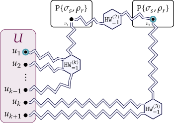
Figure 3: The gadget constructions from Lemma 6.5.

Lemma 6.5.

Let $\sigma$ and $\rho$ denote sets such that $\mathtt{HW}_{=1}^{(1)}$, $\mathtt{HW}_{=1}^{(2)}$, and $\mathtt{HW}_{=1}^{(3)}$ can be realized. Then, for all $k\geq 1$, the relation $\mathtt{HW}_{=1}^{(k)}$ can be realized by a gadget of size $\mathcal{O}(k)$.

Proof 6.6.

We use the same ideas as in the proof of [MSS21, Lemma 4.4], which uses a simple approach of obtaining a higher degree relation by combining $\mathtt{HW}_{=1}^{(2)}$ and $\mathtt{HW}_{=1}^{(3)}$ relations in a path-like manner.

Concretely, we proceed by strong induction. The base cases, $1\leq k\leq 3$ hold by assumption.

For the induction step $(k\geq 4)$, we assume that we can realize the relation for all arities from $1$ to $k$, and show that we can realize the relation for arity $k+1$. We first describe the gadget construction; then we argue about its properties. Also consult Figure 3 for a visualization of the construction.

Denote by $u_{1},\dots,u_{k+1}$ the vertices of the relation scope. First, we set $s=\min\sigma\in\sigma$ and $r=\min\rho\in\rho$, and we add to the graph two independent copies of the gadget from Section 6 for $s$ and $r$; call the portal vertices of said gadgets $v_{1}$ and $v_{2}$, respectively. Next, we add the relation $\mathtt{HW}_{=1}^{(k)}$ with scope $u_{1},\dots,u_{k-1},v_{1}$ to the graph. Then, we add the relation $\mathtt{HW}_{=1}^{(2)}$ with scope $v_{1},v_{2}$ to the graph. After that, we add the relation $\mathtt{HW}_{=1}^{(3)}$ with scope $v_{2},u_{k},u_{k+1}$ to the graph. Finally, we replace all relations with the respective realization gadgets, which exist by assumption. For the rest of this proof, call the resulting graph $G$.

Claim 8.

The graph $G$ realizes the $\mathtt{HW}_{=1}^{(k+1)}$ relation.

First, assume that no vertex of the relation scope is selected. In this case, both $v_{1}$, and $v_{2}$ must be selected, which is not possible due to the $\mathtt{HW}_{=1}^{(2)}$ relation.

Next, it is not possible that two vertices of $u_{1},\dots,u_{k-1}$ or two vertices of $u_{k},u_{k+1}$ are selected, due to the $\mathtt{HW}_{=1}^{(k)}$ and $\mathtt{HW}_{=1}^{(3)}$ relations. If one vertex of $u_{1},\dots,u_{k-1}$ and one vertex of $u_{k}$ and $u_{k+1}$ are selected, then both $v_{1}$, and $v_{2}$ cannot be selected, which is once again impossible in any solution.

Finally, if one vertex of $u_{1},\dots,u_{k+1}$ is selected, then exactly one of $v_{1}$ and $v_{2}$ must be selected, and all relations are fulfilled. Moreover, the vertices $v_{1}$ and $v_{2}$ can always receive a feasible number of neighbors, regardless of their selection status.

To conclude the proof, we analyze the size of the gadget. The gadgets for arities $1$, $2$ and $3$, and the gadgets from Section 6 have constant size each. Hence, the size of the gadget grows only by a constant amount as we go from one arity to the next, proving that the size of the gadget for arity $k$ is linear in $k$.

With Corollaries 6.3 and 6.5 at hand, we can now finally prove the main result of this section, that is, prove Definition 2.6 which we restate here for convenience.

Proof 6.7.

Let $\sigma$ and $\rho$ denote sets as in the statement of the lemma. Further, let $I_{1}$ denote an instance of $(\sigma,\rho)\mathchar 45\relax$DomSet${}^{\text{Rel}}$, let pw denote the pathwidth of the graph corresponding to $I_{1}$, and let $d$ denote the arity of the graph corresponding to $I_{1}$.

First, we apply Definition 6.1 to obtain an equivalent instance $I_{2}$ of $(\sigma,\rho)\mathchar 45\relax$DomSet${}^{\mathtt{HW}_{=1}}$ with pathwidth $\textup{{pw}}+\mathcal{O}(1)$ and arity $2^{d}+1$. By Corollaries 6.3 and 6.5, we can replace all remaining relations of the graph with their realizations. To do this, observe that any remaining relation is a $\mathtt{HW}_{=1}$ relation. To replace such a relation with a graph, we add the graph that realizes this relation, and unify its portal vertices with the vertices of the relation. Write $I_{3}$ to denote the resulting instance of $(\sigma,\rho)\mathchar 45\relax$DomSet.

Claim 9.

The instances $I_{2}$ and $I_{3}$ are equivalent.

First, assume that $I_{2}$ is a yes-instance. Then, selecting the same vertices that are selected in $I_{2}$, and extending this solution to the newly added graphs results in a solution for instance $I_{3}$. Because all relations of $I_{2}$ are fulfilled, such an extension is indeed possible by Definition 6.2.

Now, assume that $I_{3}$ is a yes-instance. Since no solution can select neighbors of vertices of $I_{3}$ that were not yet present in $I_{2}$, restricting the solution of $I_{3}$ to graph $I_{2}$ ensures that all vertices of $I_{2}$ receive a feasible number of neighbors. Moreover, the gadgets that were added to replace the relations ensure that exactly one vertex of each relation of $I_{2}$ must be selected in any solution, hence, this solution also fulfills all relations.

Claim 10.

The instance $I_{3}$ has a pathwidth of $\textup{{pw}}+\mathcal{O}(2^{d})$.

Recall from Definition 5.8 that the pathwidth of $I_{2}$ is defined as the pathwidth of the graph obtained by forming a clique out of all vertices in the relation scope for each relation. Let $\hat{I}_{2}$ denote the graph that is obtained from $I_{2}$ by applying the aforementioned transformation. Consider a path decomposition of $\hat{I}_{2}$. For any relation, there exists a bag of the decomposition in which all vertices of the relation are present. We can duplicate this bag and reconnect the bags in the natural way. Then, we simply add all vertices of the gadget that realizes the relation to the duplicated bag. It is easy to see that one can obtain a path decomposition of $I_{3}$ by performing this operation for each relation such that we never add the vertices of two realization gadgets to the same bag. The width of this decomposition is the width of the decomposition of $I_{2}$ plus the size of the largest gadget that was added to the graph. Using Lemma 6.5, we observe that this results in a decomposition of width $\textup{{pw}}+\mathcal{O}(2^{d})$, as desired. Combining 9 and 10, we obtain the claimed result.

6.1 Realizing $\mathtt{HW}_{\in\rho-\min\rho+1}$

In this section, we construct gadgets that realize $\mathtt{HW}_{\in\rho-\min\rho+1}$. Formally, we prove Section 2.2, which we restate here for convenience.

(a) The case $\min\rho\geq 2$ illustrated for $\min\sigma=1,\min\rho=3$.

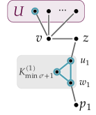
(b) The case $\min\rho=1,\min\sigma\geq 2$ illustrated for $\min\sigma=2,\min\rho=1$ and $r=1$.

(c) The case $\min\rho=\min\sigma=1$ illustrated for $r=1,s=1$.

(d) The case $\min\rho=1,\min\sigma=0$.

Figure 4: The gadget constructions from Section 2.2. In each sketched construction we mark vertices corresponding to a feasible solution within the gadget. From the relation scope $U$, we select an arbitrary vertex.

Proof 6.8.

We consider different cases, depending on $\sigma$ and $\rho$. Note that $\sigma$, $\rho$ being difficult implies that ${\mathrm{m}}\geq 3$ and $\min\rho\geq 1$.

• If $\min\rho\geq 2$, then we use 11.

• If $\min\rho=1$ and $\min\sigma\geq 2$, then we use 12.

• If $\min\rho=1$, $\min\sigma=1$, then we use 13.

• If $\min\rho=1$, $\min\sigma=0$, then we use 14.

Consult Figure 4 for a visualization of the gadgets used in the different cases of the proof.

In the following, we describe the gadgets in the strongest-possible way, that is, we describe the minimal requirements for the gadgets to work.

We start with the first case where $\min\rho\geq 2$. Clearly, ${\mathrm{m}}\geq 3$ implies that $\min\sigma+1\notin\sigma$.

Claim 11.

Let $\sigma$ and $\rho$ be arbitrary non-empty sets such that $\min\rho\geq 2$ and $\min\sigma+1\notin\sigma$. Then, $\mathtt{HW}_{\in\rho-\min\rho+1}$ is realizable.

For all $i\in\bm{[}\,1\,\bm{.\,.}\,\min\rho-1\,\bm{]}$, we create a clique $K_{\min\sigma+1}^{(i)}$ on $\min\sigma+1$ vertices. We create a vertex $v$ that is made adjacent to all vertices in the scope of the relation. Finally, we select a vertex $u^{(i)}$ from the clique $K_{\min\sigma+1}^{(i)}$, and make $v$ adjacent to $u^{(i)}$ for all $i\in\bm{[}\,1\,\bm{.\,.}\,\min\rho-1\,\bm{]}$.

The correctness relies on the fact that all vertices of each clique must be selected in a solution. To see this, fix some $i\in\bm{[}\,1\,\bm{.\,.}\,\min\rho-1\,\bm{]}$ and consider the clique $K_{\min\sigma+1}^{(i)}$.

If $\min\sigma+1=1$, then the clique consists of a single vertex $u^{(i)}$ that must be selected since $u^{(i)}$ only has a single neighbor, and if the vertex would be unselected, it would need at least two neighbors because of $\min\rho\geq 2$.

If $\min\sigma+1=2$, then the clique consists of two vertices connected by an edge. Let $w$ be the vertex of the clique that is not $u^{(i)}$. Since $w$ has only a single neighbor, vertex $w$ must be selected. But, since $\min\sigma=1$, this means that also $u^{(i)}$, the only neighbor of $w$, must be selected.

If $\min\sigma+1\geq 3$, assume that some vertex $v^{(i)}$ of the clique that is not $u^{(i)}$ is not selected in a solution. Then, $v^{(i)}$ must have two selected neighbors in the clique. At least one of them, denote it by $w^{(i)}$, must be different from $u^{(i)}$, Hence, $w^{(i)}$ is selected and requires $\min\sigma$ selected neighbors, which implies that all vertices of the clique must be selected, contradicting that $v^{(i)}$ is not selected.

By the previous argument vertex $v$ is adjacent to a vertex $u^{(i)}$ such that $u^{(i)}$ has exactly $\min\sigma$ selected neighbors in the clique. Since $\min\sigma+1\not\in\sigma$, vertex $v$ cannot be selected. Furthermore, $v$ is adjacent to $\min\rho-1$ vertices that are selected, and we know that $\min\rho-1\not\in\rho$. Thus, at least one vertex in the scope of the relation must be selected, so that $v$ can have enough neighbors. Moreover, exactly $r$ vertices from the scope must be selected where $r+\min\rho-1\in\rho$.

For all the remaining cases we assume that $\min\rho=1$. We proceed with the case where $\min\sigma\geq 2$.

Claim 12.

Let $\sigma$ and $\rho$ be arbitrary non-empty sets such that $\min\rho=1$, there exists an $r\in\rho$ with $r+1\notin\rho$, $\min\sigma\geq 2$, and $\min\sigma+1\notin\sigma$. Then, $\mathtt{HW}_{\in\rho}$ is realizable.

Observe that in our case choosing $r=\min\rho$ is possible. The gadget contains the $r+2$ vertices $v,z,p_{1},\dots,p_{r}$ and $r$ cliques $K^{(i)}_{\min\sigma+1}$ on $\min\sigma+1$ vertices each where $i\in\bm{[}\,1\,\bm{.\,.}\,r\,\bm{]}$, and $u_{i}$ and $w_{i}$ denote two distinct vertices of the clique $K^{(i)}_{\min\sigma+1}$. We make $v$ adjacent to all vertices of the scope and to $z$. Vertex $z$ is adjacent to all $u_{i}$ and vertex $w_{i}$ is adjacent to $p_{i}$ for all $i$.

In any solution, all vertices of each clique $K^{(i)}_{\min\sigma+1}$ must be selected due to vertex $p_{i}$: Vertex $p_{i}$ has only a single neighbor and hence, cannot be selected as $\min\sigma\geq 2$. Moreover, since $\min\rho=1$, the unique neighbor $w_{i}$ of $p_{i}$ must also be selected. The selected vertex $w_{i}$ then needs $\min\sigma$ selected neighbors, and so the whole clique must be selected. Then, vertex $u_{i}$ has $\min\sigma$ selected neighbors, which implies that its only other neighbor $z$ cannot be selected. Since the unselected vertex $z$ already has $r$ selected neighbors $u_{i}$, vertex $v$ cannot be selected as $r+1\notin\rho$. However, as $v$ is unselected and has no selected neighbors, it requires to have $t$ selected neighbors for some $t\in\rho$ which have to stem from the scope of the relation.

Next we change the requirement for $\min\sigma$ by assuming $\min\sigma=1$.

Claim 13.

Let $\sigma$ and $\rho$ be arbitrary non-empty sets such that $\min\rho=1$, there exists an $r\in\rho$ with $r+1\notin\rho$, $\min\sigma=1$, $\min\sigma+1\notin\sigma$, and there is an $s\in\sigma$ with $s+1,s+2\notin\sigma$. Then $\mathtt{HW}_{\in\rho}$ is realizable.

Observe that this covers our case by setting $r=1$ and $s=1$ as ${\mathrm{m}}\geq 3$. Assume we can construct a gadget $F$ where a distinguished vertex $p$ is forced to be not selected, and the only possible solution also provides exactly one selected neighbor for this vertex $p$. Then we can realize the relation as follows. Create $r$ copies of $F$ which we denote by $F_{1},\dots,F_{r}$ where we identify all vertices $p_{1},\dots,p_{r}$ with a new vertex $p$ We additionally add a vertex $v$ and make $v$ adjacent to all vertices in the scope of the relation and $p$.

By the properties of the gadget $F$, the vertex $p$ is not selected and has one neighbor in each copy $F_{i}$. Hence, vertex $v$ cannot be selected as $r+1\notin\rho$. Therefore, the number of vertices that are selected from the scope must be $t$ for some $t\in\rho$.

It remains to construct the gadget we assumed to exist above. For this we introduce $2s+3$ vertices $p,q,w$ and $u_{1},v_{1},\dots,u_{s},v_{s}$ where $p,q,w$ are connected to a path and $q,u_{i},v_{i}$ are also connected to form a path.

Since $\min\rho=\min\sigma=1$, all vertices $u_{i}$ must be selected because of the requirement of each $v_{i}$. Moreover, because the only neighbor of $w$ is $q$, vertex $q$ must be selected as well. Hence, as $\min\sigma+1\notin\sigma$ and $q$ is selected, each vertex $u_{i}$ forces $v_{i}$ to not be selected. With this selection vertex $q$ has $s$ neighbors. Since $s+1,s+2\notin\sigma$, it is not possible to select any of the vertices $w$ and $p$ which have one selected neighbor each.

This concludes the construction of the auxiliary gadget $F$ with $p$ as the distinguished vertex.

For the remaining case we now assume that $\min\sigma=0$.

Claim 14.

Let $\sigma$ and $\rho$ be arbitrary non-empty sets such that $\min\rho=1$, and $2,3\not\in\rho$, $\min\sigma=0$, and $\min\sigma+1\notin\sigma$. Then $\mathtt{HW}_{\in\rho}$ is realizable.

Observe that our case is covered since ${\mathrm{m}}\geq 3$, $\min\rho=1$ and $\min\sigma=0$ implies all required conditions. We start by creating a star graph $S_{3}$ with $3$ leaves. Let $c$ be the center of the star. Add a vertex $v$ to the graph, and make $v$ adjacent to one leaf of $S_{3}$, and to all vertices in the scope of the relation.

We first argue that in any solution, vertex $c$ must be selected, and furthermore, all of its neighbors cannot be selected. Towards a contradiction, assume that $c$ is not selected. Then, there are two leaves of $c$ that must be selected to become happy. However, for $c$, two out of three of its neighbors are now selected, and $2\not\in\rho,3\not\in\rho$. Thus, $c$ must be selected in any solution. The leaves of $c$ that have no other neighbors cannot be selected now, as they have selected neighbor $c$ and $1\not\in\sigma$.

Consider the leaf $\ell$ of $S_{3}$ that is a neighbor of $v$. This leaf has two neighbors, one of which is selected. As $c$ is selected and $1\notin\sigma$, vertex $\ell$ cannot be selected. Furthermore, $v$ cannot be selected either, because selecting $v$ would give $\ell$ two selected neighbors and $2\not\in\rho$. Thus, $v$ is not selected and requires at least one more selected vertex from the scope of the relation.

Finally, we can make all vertices of the gadget happy if $r\in\rho$ vertices of the relation scope are selected. In that case, $c$ is the only gadget vertex that must be selected. The leaves of $c$ are happy, because they have a single selected neighbor and are unselected. Furthermore, vertex $v$ is happy, because it has $r$ selected neighbors in the scope of the relation.

This finishes the proof of Section 2.2 by combining 11, 12, 13, and 14.

7 Turn the Lights Off!

As already mentioned in the introduction the decision version of Lights Out! is solvable in polynomial-time by Gaussian elimination on the corresponding set of linear equations [Sut89, AF98]. However, as the minimization version of the problem is NP-complete when $\rho=\{x\in\mathbb{Z}_{\geq 0}\mid x\equiv_{2}1\}$ [Sut88, CKG01, HKT00b], it is open whether our algorithm from Section 1 is optimal or not. In this section we answer this question in the positive by formally proving Section 1.

*

Recall that we denote by Reflexive-AllOff the minimization version of $(\sigma,\rho)\mathchar 45\relax$DomSet where $\sigma=\{x\in\mathbb{Z}_{\geq 0}\mid x\equiv_{2}0\}$ and $\rho=\{x\in\mathbb{Z}_{\geq 0}\mid x\equiv_{2}1\}$, and by AllOff the variant where $\sigma=\rho=\{x\in\mathbb{Z}_{\geq 0}\mid x\equiv_{2}1\}$.

We use the NP-hardness result by Sutner in [Sut88, Theorem 3.2] as a basis and strengthen our results by directly proving the bounds for the larger parameter pathwidth. We consider AllOff in Section 7.2 and Reflexive-AllOff in Section 7.1. The proof of Section 1 then directly follows from the combination of the main results of the aforementioned sections.

7.1 Lower Bound for Reflexive-AllOff

In the following we prove the lower bound for Reflexive-AllOff by a reduction from $k$-SAT to an equivalent instance of Reflexive-AllOff with small pathwidth.

Theorem 7.1.

For all $\varepsilon>0$, there is no algorithm deciding in time $(2-\varepsilon)^{\textup{{pw}}}\cdot n^{\mathcal{O}(1)}$ whether there exists a solution of size at most $k$ for a given Reflexive-AllOff instance even if we are given a path decomposition of width pw, unless SETH fails.

Proof 7.2.

We prove the lower bound by a reduction from CNF-SAT. Fix some $\varepsilon>0$ for this and let $k$ be the smallest integer such that $k$-SAT does not have a $(2-\varepsilon)^{n}\cdot(n+m)^{\mathcal{O}(1)}$ algorithm where $n$ is the number of variables and $m$ the number of clauses.

Consider an arbitrary $k$-SAT formula $\varphi$ with $n$ variables $x_{1},\dots,x_{n}$ and $m$ clauses $C^{1},\dots,C^{m}$ as input. In the following we construct a graph $G_{\varphi}$ as an instance of Reflexive-AllOff. The graph is build based on variable gadgets, clause gadgets, and a single negation gadget.

We first construct the gadgets and then describe how they are connected. For every variable $x_{i}$ where $i\in\bm{[}\,1\,\bm{.\,.}\,n\,\bm{]}$, the variable gadget $V_{i}$ consists of the two vertices $v_{i}$ and $\overline{v}_{i}$ that are connected by an edge.

For every clause $C^{j}=\lambda^{j}_{1}\lor\dots\lor\lambda^{j}_{k}$ where $j\in\bm{[}\,1\,\bm{.\,.}\,m\,\bm{]}$, the clause gadget $D^{j}$ contains the following vertices and edges. There are $k$ literal vertices $t^{j}_{1},\dots,t^{j}_{k}$ where each vertex corresponds to one literal of the clause. Moreover, the gadget $D^{j}$ contains so-called subset vertices $s^{j}_{L}$ for all $L\subsetneq\bm{[}\,1\,\bm{.\,.}\,k\,\bm{]}$, that is, for every proper subset of the literals of the clause, there exists a vertex labeled with this subset (and the gadget index). For each subset $L\subsetneq\bm{[}\,1\,\bm{.\,.}\,k\,\bm{]}$, the subset vertex $s^{j}_{L}$ is connected to the literal vertex $t^{j}_{\ell}$ if and only if $\ell\in L$. Moreover, all subset vertices together form a clique on $2^{k}-1$ vertices.

The negation gadget consists of three vertices $q_{0}$, $q_{1}$, and $q_{2}$ that are connected to a path on three vertices with $q_{1}$ in the middle.

As a last step it remains to connect the vertices of the different gadgets. Intuitively, each literal vertex of the clause gadget is connected to the corresponding variable vertex of the variable gadgets. Consider literal $\lambda^{j}_{\ell}$, that is, the $\ell$th literal in the $j$th clause. If this literal is positive, i.e., if $\lambda^{j}_{\ell}=x_{i}$ for some variable $x_{i}$, then the vertex $t^{j}_{\ell}$ is adjacent to vertex $v_{i}$. If the literal is negative, i.e., if $\lambda^{j}_{\ell}=\lnot x_{i}$ for some variable $x_{i}$, then the vertex $t^{j}_{\ell}$ is also adjacent to vertex $v_{i}$ but additionally also to vertex $q_{1}$.

This concludes the description of $G_{\varphi}$. See Figure 5 for an illustration of the clause gadget and the negation gadget. To prove the correctness of this reduction we set $m+n+1$ as the upper bound for the number of selected vertices.

Figure 5: A depiction of the clause gadget for the clause $x_{1}\lor x_{2}\lor\neg x_{3}$ as well as the negation gadget. Some indices are omitted for simplicity.

Claim 15.

If $\varphi$ is a yes-instance of $k$-SAT, then $(G_{\varphi},n+m+1)$ is a yes-instance of Reflexive-AllOff.

Let $\pi$ be a satisfying assignment for the $k$-SAT formula $\varphi$. We select the following vertices:

In the variable gadget of variable $x_{i}$, we select $v_{i}$ if $\pi(x_{i})=1$ and $\overline{v}_{i}$ otherwise.

In the clause gadget of clause $C^{j}$, let $L\subsetneq\bm{[}\,1\,\bm{.\,.}\,k\,\bm{]}$ be the set of literal indices of this clause that are not satisfied. (This is well-defined as $\pi$ is a satisfying which means that not all literals are unsatisfied.) We select vertex $s^{j}_{L}$.

We select vertex $q_{1}$ from the negation gadget. Let $S$ denote the set of all selected vertices.

Since we select exactly one vertex from each gadget, the size of $S$ is precisely $n+m+1$. It remains to prove that $S$ is indeed a solution, that is, $S$ is a $(\sigma,\rho)$-set where $\sigma=\{x\in\mathbb{Z}_{\geq 0}\mid x\equiv_{2}0\}$ and $\rho=\{x\in\mathbb{Z}_{\geq 0}\mid x\equiv_{2}1\}$.

First, consider the vertices of the negation gadget. Since only vertex $q_{1}$ is selected, the vertices $q_{0}$ and $q_{2}$ have exactly one selected neighbors. As none of the literal vertices are selected, vertex $q_{1}$ is adjacent to zero selected vertices.

Consider any vertex of the variable gadgets and observe that none of them have a selected neighbor outside the gadget. By our choice of $S$, exactly one of the two vertices is selected and has no selected neighbors, while the other vertex is not selected and has exactly one selected neighbor, the one in the variable gadget.

It remains to check the vertices of the clause gadget. For the subset vertices we notice that in every clause gadget exactly one of them is selected. Recall that all subset vertices of one clause are connected to each other, and they are not connected to any other vertices outside the gadget but only to the unselected literal vertices of the gadget. This implies that exactly one of the subset vertices is selected and has no selected neighbors, whereas the other subset vertices are not selected and have exactly one selected neighbor.

Next we check the literal vertices. Consider a positive literal, say $\lambda^{j}_{\ell}=x_{i}$. By assumption $t^{j}_{\ell}$ is unselected and has vertex $v_{i}$ as neighbor if $\pi(x_{i})=1$. In this case no subset vertex $s^{j}_{L}$ with $\ell\in L$ is selected by definition of $S$. Hence, the vertex has exactly one selected neighbor. If $\pi(x_{i})=0$, then the literal does not satisfy the clause and hence, by the definition of $S$, a vertex $s^{j}_{L}$ is selected where $\ell\in L$.

As a last step we check the literal vertices corresponding to negated variables, say $t^{j}_{\ell}=\lnot x_{i}$. Once more, this vertex is not selected but always adjacent to the selected vertex $q_{1}$ from the negation gadget. If $\pi(x_{i})=1$, then also the neighboring vertex $v_{i}$ is selected. However, this is not a problem since in this case the literal does not satisfy the clause and hence, a subset vertex $s^{j}_{L}$ with $\ell\in L$ must be selected. Thus, the literal vertex is adjacent to three selected vertices. If $\pi(x_{i})=0$, then the literal satisfies the clause and no subset vertex $s^{j}_{L}$ with $\ell\in L$ is selected; the literal vertex has exactly one selected neighbor.

We conclude that every selected vertex of the graph has no selected neighbors, whereas every unselected vertex has either exactly one or exactly three selected neighbors.

As a next step we show the reverse direction of the correctness.

Claim 16.

If $(G_{\varphi},n+m+1)$ is a yes-instance of Reflexive-AllOff, then $\varphi$ is a yes-instance of $k$-SAT.

Consider a solution $S$ of the Reflexive-AllOff instance of size at most $n+m+1$. Recall that $S$ is a $(\sigma,\rho)$-set for $G_{\varphi}$ where $\sigma=\{x\in\mathbb{Z}_{\geq 0}\mid x\equiv_{2}0\}$ and $\rho=\{x\in\mathbb{Z}_{\geq 0}\mid x\equiv_{2}1\}$.

In the negation gadget at least one vertex must be selected as $q_{0}$ and $q_{2}$ must be selected themselves or require one selected neighbor which can only be $q_{1}$. Similarly, in each variable gadget $V_{i}$, the set $S$ contains at least one vertex; vertex $\overline{v}_{i}$ is either selected itself or it requires a selected neighbor (which must be $v_{i}$).

In each clause gadget $D^{j}$, we must also select at least one vertex which must be a subset vertex. Indeed, the subset vertex $s^{j}_{\varnothing}$ must either be selected or have a selected neighbor. As all neighbors of this subset vertex are also subset vertices, the claim follows.

Hence, we see that any solution $S$ of size at most $n+m+1$ must select exactly one vertex of each variable gadget, as well as exactly one subset vertex of each clause gadget, and vertex $q_{1}$ of the negation gadget.

Based on these observations we define an assignment $\pi$ for the formula $\varphi$ by setting $\pi(x_{i})=1$ if and only if $v_{i}\in S$ and $\pi(x_{i})=0$ otherwise.

In the following we prove that $\pi$ satisfies $\varphi$. For this consider an arbitrary clause $C^{j}$. By the above discussion, we know that there is some selected subset vertex $s^{j}_{L}$ of the clause gadget $D^{j}$. Since $L\subsetneq\bm{[}\,1\,\bm{.\,.}\,k\,\bm{]}$, there is, by the construction of $G_{\varphi}$, a literal vertex $t^{j}_{\ell}$ where $\ell\in\bm{[}\,1\,\bm{.\,.}\,k\,\bm{]}\setminus L$. Since this vertex $t^{j}_{\ell}$ is not selected, it must have an odd number of neighbors in $S$. We first consider the case that the corresponding literal $\lambda^{j}_{\ell}$ is positive, that is, $\lambda^{j}_{\ell}=x_{i}$ for some variable $x_{i}$. In this case the only selected neighbor of $t^{j}_{\ell}$ is $v_{i}$. From $v_{i}\in S$ the definition of $\pi$ gives $\pi(x_{i})=1$ which implies that the clause $C^{j}$ is satisfied by literal $\lambda^{j}_{\ell}$. Now consider the case when $\lambda^{j}_{\ell}=\lnot x_{i}$ for some variable $x_{i}$. In this case vertex $t^{j}_{\ell}$ is adjacent to the selected vertex $q_{1}$ of the negation gadget, by the construction of $G_{\varphi}$ and the above observations. As the literal vertex is still unselected and only adjacent to unselected subset vertices and one additional variable vertex, the variable vertex $v_{i}$ cannot be selected. Hence, the definition of the assignment $\pi$ gives $\pi(x_{i})=0$ which directly implies that the clause $C^{j}$ is satisfied by the literal $\lambda^{j}_{\ell}$.

Before we combine all parts of the proof to obtain the lower bound, we first provide a bound on the pathwidth of the constructed graph.

Claim 17.

$G_{\varphi}$ has pathwidth at most $2^{k}+k+n$.

If we delete vertex $q_{1}$ and, for all $i\in\bm{[}\,1\,\bm{.\,.}\,n\,\bm{]}$, the variable vertex $v_{i}$, then the graph decomposes into small components of size at most $2^{k}-1+k$. This allows us to get a path decomposition of small width.

Concretely, we create a node for every variable gadget, clause gadget, and the negation gadget. We add the vertices of the corresponding gadgets to the bag of the node. We connect these nodes in an arbitrary way to form a path. As a last step we extend all bags by adding the vertices in $\{v_{i}\mid i\in\bm{[}\,1\,\bm{.\,.}\,n\,\bm{]}\}\cup\{q_{1}\}$. It is easy to see that this is a valid path decomposition.

The bags corresponding to the variable gadgets have size $1+(n+1)$ and the bags of the clause gadgets have size $2^{k}-1+k+(n+1)$. Finally, the bag of the negation gadget has size $2+(n+1)$. Hence, the pathwidth of the graph is at most $\max(2^{k}+k+n-1,n+2)\leq 2^{k}+k+n$.

Recall that we fixed some $\varepsilon>0$ and set $k$ to the smallest integer such that $k$-SAT does not have an algorithm with running time $(2-\varepsilon)^{n}\cdot n^{\mathcal{O}(1)}$ where $n$ is the number of variables. For a given $k$-SAT formula $\varphi$ with $n$ variables and $m$ clauses we constructed an equivalent Reflexive-AllOff instance $(G_{\varphi},n+m+1)$ together with a path decomposition.

Towards a contradiction, assume that Reflexive-AllOff can be solved in time $(2-\varepsilon)^{\textup{{pw}}}\cdot N^{\mathcal{O}(1)}$. Applying this algorithm to the constructed instance $(G_{\varphi},n+m+1)$, yields, by using 15, 16, and 17, an algorithm for $k$-SAT with running time

$$(2-\varepsilon)^{\textup{{pw}}}\cdot(n+m)^{\mathcal{O}(1)}=(2-\varepsilon)^{2^{k}+k+n}\cdot(n+m)^{\mathcal{O}(1)}\leq(2-\varepsilon)^{n}\cdot(n+m)^{\mathcal{O}(1)}$$

as the constant $k$ only depends on the fixed value $\varepsilon$. This directly contradicts SETH and finishes the proof.

7.2 Lower Bound for AllOff

In the previous section we have seen the lower bound for Reflexive-AllOff. In this section we focus on the non-reflexive version AllOff instead. Recall, that when representing this problem as $(\sigma,\rho)\mathchar 45\relax$DomSet we have $\sigma=\rho=\{x\in\mathbb{Z}_{\geq 0}\mid x\equiv_{2}1\}$, that is, every vertex needs and odd number of selected neighbors independent of whether the vertices are themselves selected or not.

We again use the ideas by Sutner [Sut88] which allows a reduction in a similar spirit as the previous one. The main difference is that the subset vertices now do not form a clique. As there are naturally other minor modifications we present the full proof.

Theorem 7.3.

For all $\varepsilon>0$, there is no algorithm that for a given instance of AllOff decides in time $(2-\varepsilon)^{\textup{{pw}}}\cdot n^{\mathcal{O}(1)}$ whether there exists a solution of size at most $k$ even if we are given a path decomposition of width pw, unless SETH fails.

Proof 7.4.

Similar to Theorem 7.1, we prove the bound by a reduction from CNF-SAT. For this fix some $\varepsilon>0$ and let $k$ be the smallest integer such that $k$-SAT has no $(2-\varepsilon)^{n}\cdot(n+m)^{\mathcal{O}(1)}$ algorithm under SETH where $n$ is the number of variables and $m$ the number of clauses.

Let $\varphi$ be an arbitrary $k$-SAT instance with $n$ variables $x_{1},\dots,x_{n}$ and $m$ clauses $C^{1},\dots,C^{m}$ as input. We construct a graph $G_{\varphi}$ that consists of variable and clause gadgets. See Figure 6 for an illustration of the construction.

For every variable $x_{i}$ where $i\in\bm{[}\,1\,\bm{.\,.}\,n\,\bm{]}$, the graph $G_{\varphi}$ contains a variable gadget $V_{i}$. Gadget $V_{i}$ consists of a cycle of length four on the four vertices $v_{i}$, $w_{i}$, $\overline{v}_{i}$, and $\overline{w}_{i}$ (in this order).

For every clause $C_{i}=\lambda^{j}_{1}\lor\dots\lor\lambda^{j}_{k}$ where $j\in\bm{[}\,1\,\bm{.\,.}\,m\,\bm{]}$, the graph $G_{\varphi}$ contains a clause gadget $D^{j}$. This gadget $D^{j}$ contains $k$ literal vertices $t^{j}_{1},\dots,t^{j}_{k}$, that is, one distinguished vertex for every literal of the clause. Additionally, $D^{j}$ contains, for every subset $L\subsetneq\bm{[}\,1\,\bm{.\,.}\,k\,\bm{]}$, a so called subset-vertex $s^{j}_{L}$, that is, for every proper subset of the literals of the clause, there exists a vertex labeled with the subset (and the gadget index). These subset vertices are used to indicate which literals of the clause are not satisfied by the encoded assignment. As a last vertex there is an additional vertex $h^{j}$ (for happy) in $D^{j}$. There are two different groups of edges in the gadget; first, each subset vertex $s^{j}_{L}$ is connected to each literal vertex $t^{j}_{\ell}$ if and only if $\ell\in L$. Second, the vertex $h^{j}$ is connected to all subset vertices of the gadget $D^{j}$.

As a last step of the construction we describe the edges encoding the appearance of variables in the clauses. Intuitively each literal vertex of the clause gadget is connected to the corresponding variable vertex of the variable gadgets. Formally, if the $\ell$th literal of the $j$th clause is positive, i.e., if $\lambda^{j}_{\ell}=x_{i}$ for some variable $x_{i}$, then vertex $t^{j}_{\ell}$ is adjacent to vertex $v_{i}$. If the $\ell$th literal is negative, i.e., if $\lambda^{j}_{\ell}=\neg x_{i}$ for some variable $x_{i}$, then vertex $t^{j}_{\ell}$ is again adjacent to vertex $v_{i}$ but also to vertex $h^{j}$.

This concludes the description of $G_{\varphi}$. We prove in the following that the AllOff instance $(G_{\varphi},2m+2n)$ is equivalent to the input instance $\varphi$ of $k$-SAT.

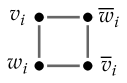
(a) A depiction of the variable gadget.

(b) A depiction of the clause gadget for the clause $x_{1}\lor x_{2}\lor\neg x_{3}$.

Figure 6: A depiction of a literal gadget and a clause gadget from the proof of the lower bound for AllOff. Some indices are omitted for simplicity.

We first show that if the $k$-SAT formula $\varphi$ is satisfiable, then the constructed AllOff instance is a yes-instance.

Claim 18.

If $\varphi$ is a yes-instance of $k$-SAT, then $(G_{\varphi},2m+2n)$ is a yes-instance of AllOff.

Consider a satisfying assignment $\pi$ for $\varphi$. We select the following vertices:

For all $i\in\bm{[}\,1\,\bm{.\,.}\,n\,\bm{]}$, if $\pi(x_{i})=1$, then we select the two vertices $v_{i}$ and $w_{i}$. If $\pi(x_{i})=0$, then we select the other two vertices of the variable gadget, which are $\overline{v}_{i}$ and $\overline{w}_{i}$.

For all $j\in\bm{[}\,1\,\bm{.\,.}\,m\,\bm{]}$, we select in the clause gadget the vertex $h^{j}$. Moreover, let $L\subsetneq\bm{[}\,1\,\bm{.\,.}\,k\,\bm{]}$ be the set of all positions of the literals of the clause that are not satisfied by $\pi$. Since the clause is satisfied by the assignment, the set $L$ cannot contain all literals of the clause. Thus, there is a subset vertex $s^{j}_{L}$ corresponding to this set $L$. We select this vertex $s^{j}_{L}$. Let $S$ denote the set of all selected vertices. Clearly this set contains exactly $2n+2m$ vertices as we select exactly two vertices from every gadget. It remains to show that $S$ is indeed a solution, that is, every vertex of $G_{\varphi}$ has an odd number of neighbors in $S$.

Consider any vertex of the variable gadgets and observe that none of them have a selected neighbor outside the gadget. With this it is easy to see that each vertex of a variable gadget has exactly one selected neighbor in $S$.

Each subset vertex of a clause gadget $D^{j}$ has exactly one selected neighbor, namely vertex $h^{j}$. Furthermore, vertex $h^{j}$ has exactly one selected neighbor, namely the selected subset vertex of the clause gadget. Now consider an arbitrary literal vertex $t^{j}_{\ell}$. First assume that the corresponding literal is positive, that is, $\lambda^{j}_{\ell}=x_{i}$ for some variable $x_{i}$. If this literal is satisfied, the vertex $v_{i}$ in the variable gadget is selected, otherwise if the literal is not satisfied, $t^{j}_{\ell}$ is a neighbor if the selected subset vertex.

Now assume that the corresponding literal is negative, that is, $\lambda^{j}_{\ell}=\lnot x_{i}$ for some variable $x_{i}$. If the variable $x_{i}$ is not satisfied by $\pi$, then the only selected neighbor of $t^{j}_{\ell}$ is $h^{j}$. If the variable $x_{i}$ is satisfied by $\pi$, then the literal $\lambda^{j}_{\ell}$ is not satisfied which implies that the literal vertex is adjacent to the selected subset vertex of this clause gadget. Moreover, vertex $t^{j}_{\ell}$ is adjacent to $v_{i}$ and thus, to three selected vertices which is a valid number.

We conclude the proof by observing that every vertex has either one or three selected neighbors and thus, we constructed a valid solution.

As a next step we prove the reverse direction of the correctness.

Claim 19.

If $(G_{\varphi},2m+2n)$ is a yes-instance of AllOff, then $\varphi$ is a yes-instance of $k$-SAT.

Consider a solution $S$ to the AllOff instance of size at most $2m+2n$. Recall that every vertex of $G_{\varphi}$ is adjacent to an odd number of vertices in $S$.

We first start with some observations about the solution $S$. In each variable gadget $V_{i}$, vertex $\overline{v}_{i}$ must have a selected neighbor in $S$ (which is either $w_{i}$ or $\overline{w}_{i}$), and this selected neighbor itself requires a selected neighbor in $S$ (which is either $v_{i}$ or $\overline{v}_{i}$). Hence, at least two vertices must be selected from each variable gadget.

In each clause gadget $D^{j}$, the vertex $s^{j}_{\varnothing}$ must have a selected neighbor which forces its only neighbor, which is vertex $h^{j}$, to be selected. As this vertex also needs a selected neighbor, one of the subset vertices of this clause gadget must be selected as well. From the given bound on the solution size, we conclude that in every variable gadget and every clause gadget exactly two vertices are selected. Moreover, from each clause gadget $D^{j}$ exactly one subset vertex, and vertex $h^{j}$ are selected.

We define the assignment $\pi$ for the variables of $\varphi$ such that $\pi(x_{i})=1$ if and only if $v_{i}\in S$ and $\pi(x_{i})=0$ otherwise.

It remains to show that $\pi$ satisfies $\varphi$. To prove this, consider an arbitrary clause $C^{j}$. Let $s^{j}_{L}$ be the selected subset vertex from the clause gadget $D^{j}$. As $L\neq\bm{[}\,1\,\bm{.\,.}\,k\,\bm{]}$ by the construction of $G_{\varphi}$, there is some literal vertex $t^{j}_{\ell}$ such that $\ell\notin L$. If the corresponding literal is positive, i.e., if $\lambda^{j}_{\ell}=x_{i}$, then $t^{j}_{\ell}$ is not adjacent to $h^{j}$. As $t^{j}_{\ell}$ must have one selected neighbor in $S$ and since the vertex is not adjacent to any selected subset vertex, the only remaining neighbor of $t^{j}_{\ell}$, i.e., vertex $v_{i}$, must be selected which implies that $\pi$ was defined such that $\pi(x_{i})=1$.

If the literal is negative, i.e., if $\lambda^{j}_{\ell}=\lnot x_{i}$, then the vertex $t^{j}_{\ell}$ is adjacent to $h^{j}$ by the construction of $G_{\varphi}$. Since $h^{j}$ is selected, vertex $t^{j}_{\ell}$ cannot have further selected neighbors as all other adjacent subset vertices are unselected. Hence, the vertex $v_{i}$ is also unselected which implies that, by the definition of $\pi$, the variable $x_{i}$ is not satisfied but the literal $\lambda^{j}_{\ell}$ is satisfied which makes the clause $C^{j}$ true.

As a last step we prove a bound on the pathwidth of the constructed graph.

Claim 20.

$G_{\varphi}$ has pathwidth at most $n+k+1$.

Intuitively the idea is as follows. If we delete all the variable vertices $v_{i}$ for all $i\in\bm{[}\,1\,\bm{.\,.}\,n\,\bm{]}$ in the variable gadgets, the graph decomposes into small components. We use this to construct a path decomposition in the following by providing a node search strategy (see e.g. [CFK⁺15, Section 7.5]).

We start by placing one searcher on each vertex $v_{i}$ for every $i\in\bm{[}\,1\,\bm{.\,.}\,k\,\bm{]}$. Each of the variable gadget can be cleaned by using $3$ additional searchers which we just place on all vertices.

For the clause gadgets we use a more complex approach to clean all vertices. Fix a clause gadget $D^{j}$ for this. We first place $k$ new searchers on the $k$ literal vertices of the gadget and one more searcher on the vertex $h^{j}$. The remaining subset vertices can then be cleaned by using one additional searcher which we put one subset vertex after the other. Repeating this procedure for all clause gadgets cleans the entire graph.

This approach uses at most $n+k+2$ searchers simultaneously. Thus, the claimed bound on the pathwidth follows immediately.

Recall that we fixed some $\varepsilon>0$ and chose $k$ as the smallest integer such that $k$-SAT has no $(2-\varepsilon)^{n}\cdot(n+m)^{\mathcal{O}(1)}$ algorithm under SETH where $n$ is the number of variables and $m$ the number of clauses. For a given $k$-SAT instance $\varphi$ with $n$ variables and $m$ clauses we constructed an equivalent AllOff instance $(G_{\varphi},2n+2m)$ together with a path decomposition.

For the sake of a contradiction, now assume that AllOff can be solved in time $(2-\varepsilon)^{\textup{{pw}}}\cdot N^{\mathcal{O}(1)}$ on graphs of size $N$. If we apply this algorithm to the constructed instance, we also solve, by 18, 19, and 20 the $k$-SAT instance in time

$$(2-\varepsilon)^{\textup{{pw}}}\cdot N^{\mathcal{O}(1)}=(2-\varepsilon)^{n+k+1}\cdot(n+m)^{\mathcal{O}(1)}=(2-\varepsilon)^{n}\cdot(n+m)^{\mathcal{O}(1)}$$

as $k$ depends only on the fixed value $\varepsilon$ and thus, only contributes a constant to the running time. This then directly contradicts SETH and finishes the proof.

Proof 7.5.

Follows from Theorems 7.1 and 7.3.

References

- [ABF+02] Jochen Alber, Hans L. Bodlaender, Henning Fernau, Ton Kloks, and Rolf Niedermeier. Fixed parameter algorithms for DOMINATING SET and related problems on planar graphs. Algorithmica, 33(4):461–493, 2002. doi:10.1007/S00453-001-0116-5.
- [AF98] Marlow Anderson and Todd Feil. Turning lights out with linear algebra. Mathematics Magazine, 71(4):300–303, 1998.
- [BBH21] Abraham Berman, Franziska Borer, and Norbert Hungerbühler. Lights out on graphs. Mathematische Semesterberichte, 68(2):237–255, 2021. doi:10.1007/s00591-021-00297-5.
- [BL16] Glencora Borradaile and Hung Le. Optimal dynamic program for r-domination problems over tree decompositions. In Jiong Guo and Danny Hermelin, editors, 11th International Symposium on Parameterized and Exact Computation, IPEC 2016, August 24-26, 2016, Aarhus, Denmark, volume 63 of LIPIcs, pages 8:1–8:23. Schloss Dagstuhl - Leibniz-Zentrum für Informatik, 2016. doi:10.4230/LIPICS.IPEC.2016.8.
- [BMOR18] Michael A. Bennett, Greg Martin, Kevin O’Bryant, and Andrew Rechnitzer. Explicit bounds for primes in arithmetic progressions. Illinois J. Math., 62(1-4):427–532, 2018. doi:10.1215/ijm/1552442669.
- [BTV13] Binh-Minh Bui-Xuan, Jan Arne Telle, and Martin Vatshelle. Fast dynamic programming for locally checkable vertex subset and vertex partitioning problems. Theor. Comput. Sci., 511:66–76, 2013. doi:10.1016/J.TCS.2013.01.009.
- [CFK+15] Marek Cygan, Fedor V. Fomin, Lukasz Kowalik, Daniel Lokshtanov, Dániel Marx, Marcin Pilipczuk, Michal Pilipczuk, and Saket Saurabh. Parameterized Algorithms. Springer, 2015. doi:10.1007/978-3-319-21275-3.
- [Cha10] Mathieu Chapelle. Parameterized complexity of generalized domination problems on bounded tree-width graphs. CoRR, abs/1004.2642, 2010. arXiv:1004.2642v5, doi:10.48550/arxiv.1004.2642.
- [Cha11] Mathieu Chapelle. Décompositions de graphes : quelques limites et obstructions. (Graphs decompositions: some limites and obstructions). PhD thesis, University of Orléans, France, 2011.
- [CHKS07] Robert Cowen, Stephen H. Hechler, John W. Kennedy, and Arthur Steinberg. Odd neighborhood transversals on grid graphs. Discrete Mathematics, 307(17-18):2200–2208, 2007. doi:10.1016/j.disc.2006.11.006.
- [CIP09] Chris Calabro, Russell Impagliazzo, and Ramamohan Paturi. The complexity of satisfiability of small depth circuits. In IWPEC, volume 5917 of LNCS, pages 75–85, 2009.
- [CJ03] Yair Caro and Michael S. Jacobson. On non-z(mod k) dominating sets. Discussiones Mathematicae Graph Theory, 23(1):189–199, 2003.
- [CK03] Yair Caro and William F. Klostermeyer. The odd domination number of a graph. Journal of Combinatorial Mathematics and Combinatorial Computing, 44:65–84, 2003.
- [CKG01] Yair Caro, William F. Klostermeyer, and John L. Goldwasser. Odd and residue domination numbers of a graph. Discussiones Mathematicae Graph Theory, 21(1):119–136, 2001. doi:10.7151/dmgt.1137.
- [CM16] Radu Curticapean and Dániel Marx. Tight conditional lower bounds for counting perfect matchings on graphs of bounded treewidth, cliquewidth, and genus. In Robert Krauthgamer, editor, Proceedings of the Twenty-Seventh Annual ACM-SIAM Symposium on Discrete Algorithms, SODA 2016, Arlington, VA, USA, January 10-12, 2016, pages 1650–1669. SIAM, 2016. doi:10.1137/1.9781611974331.CH113.
- [Cou90] Bruno Courcelle. The monadic second-order logic of graphs. i. recognizable sets of finite graphs. Inf. Comput., 85(1):12–75, 1990. doi:10.1016/0890-5401(90)90043-H.
- [FGK+09] Fedor V. Fomin, Petr A. Golovach, Jan Kratochvíl, Dieter Kratsch, and Mathieu Liedloff. Sort and search: Exact algorithms for generalized domination. Inf. Process. Lett., 109(14):795–798, 2009. doi:10.1016/J.IPL.2009.03.023.
- [FLPS16] Fedor V. Fomin, Daniel Lokshtanov, Fahad Panolan, and Saket Saurabh. Efficient computation of representative families with applications in parameterized and exact algorithms. J. ACM, 63(4):29:1–29:60, 2016. doi:10.1145/2886094.
- [FMI+23a] Jacob Focke, Dániel Marx, Fionn Mc Inerney, Daniel Neuen, Govind S. Sankar, Philipp Schepper, and Philip Wellnitz. Tight complexity bounds for counting generalized dominating sets in bounded-treewidth graphs. In Nikhil Bansal and Viswanath Nagarajan, editors, Proceedings of the 2023 ACM-SIAM Symposium on Discrete Algorithms, SODA 2023, Florence, Italy, January 22-25, 2023, pages 3664–3683. SIAM, 2023. doi:10.1137/1.9781611977554.CH140.
- [FMI+23b] Jacob Focke, Dániel Marx, Fionn Mc Inerney, Daniel Neuen, Govind S. Sankar, Philipp Schepper, and Philip Wellnitz. Tight complexity bounds for counting generalized dominating sets in bounded-treewidth graphs Part I: Algorithmic results, June 2023. arXiv:2211.04278, doi:10.48550/arxiv.2211.04278.
- [FMI+23c] Jacob Focke, Dániel Marx, Fionn Mc Inerney, Daniel Neuen, Govind S. Sankar, Philipp Schepper, and Philip Wellnitz. Tight complexity bounds for counting generalized dominating sets in bounded-treewidth graphs Part II: Hardness results, May 2023. arXiv:2306.03640, doi:10.48550/arXiv.2306.03640.
- [FY13] Rudolf Fleischer and Jiajin Yu. A survey of the game ”lights out!”. In Andrej Brodnik, Alejandro López-Ortiz, Venkatesh Raman, and Alfredo Viola, editors, Space-Efficient Data Structures, Streams, and Algorithms - Papers in Honor of J. Ian Munro on the Occasion of His 66th Birthday, volume 8066 of Lecture Notes in Computer Science, pages 176–198. Springer, 2013. doi:10.1007/978-3-642-40273-9_13.
- [GH08] Elisabeth Gassner and Johannes Hatzl. A parity domination problem in graphs with bounded treewidth and distance-hereditary graphs. Computing, 82(2-3):171–187, July 2008. doi:10.1007/s00607-008-0005-8.
- [GK07] John L. Goldwasser and William F. Klostermeyer. Odd and even dominating sets with open neighborhoods. Ars Combinatoria, 83:229–247, 2007.
- [GKT97] John L. Goldwasser, William Klostermeyer, and George Trapp. Characterizing switch-setting problems. Linear and Multilinear Algebra, 43:121–135, 1997.
- [GKTZ95] John Goldwasser, William Klostermeyer, George Trapp, and Cun-Quan Zhang. Setting switches in a grid. Technical Report TR-95-20, West Virginia University, Dept. of Statistics and Computer, 1995.
- [GP13] Alexander Giffen and Darren B. Parker. On generalizing the ”Lights Out” game and a generalization of parity domination. Ars Comb., 111:273–288, 2013.
- [HKT00a] Magnús M. Halldórsson, Jan Kratochvíl, and Jan Arne Telle. Independent sets with domination constraints. Discret. Appl. Math., 99(1-3):39–54, 2000. doi:10.1016/S0166-218X(99)00124-9.
- [HKT00b] Magnús M. Halldórsson, Jan Kratochvíl, and Jan Arne Telle. Mod-2 independence and domination in graphs. Int. J. Found. Comput. Sci., 11(3):355–363, 2000. doi:10.1142/S0129054100000272.
- [IP01] Russell Impagliazzo and Ramamohan Paturi. On the Complexity of k-SAT. J. Comput. Syst. Sci., 62(2):367–375, 2001. doi:10.1006/jcss.2000.1727.
- [KW20] Stefan Kratsch and Magnus Wahlström. Representative sets and irrelevant vertices: New tools for kernelization. J. ACM, 67(3):16:1–16:50, 2020. doi:10.1145/3390887.
- [Lam20] Michael Lampis. Finer tight bounds for coloring on clique-width. SIAM J. Discret. Math., 34(3):1538–1558, 2020. doi:10.1137/19M1280326.
- [LMS18] Daniel Lokshtanov, Dániel Marx, and Saket Saurabh. Known algorithms on graphs of bounded treewidth are probably optimal. ACM Transactions on Algorithms, 14(2):13:1–13:30, April 2018. doi:10.1145/3170442.
- [Min12] Igor Minevich. Symmetric matrices over f_2 and the lights out problem. CoRR, abs/1206.2973, 2012. arXiv:1206.2973, doi:10.48550/arxiv.1206.2973.
- [MSS21] Dániel Marx, Govind S. Sankar, and Philipp Schepper. Degrees and gaps: Tight complexity results of general factor problems parameterized by treewidth and cutwidth. In Nikhil Bansal, Emanuela Merelli, and James Worrell, editors, 48th International Colloquium on Automata, Languages, and Programming, ICALP 2021, July 12-16, 2021, Glasgow, Scotland (Virtual Conference), volume 198 of LIPIcs, pages 95:1–95:20. Schloss Dagstuhl - Leibniz-Zentrum für Informatik, 2021. doi:10.4230/LIPICS.ICALP.2021.95.
- [MSS22] Dániel Marx, Govind S. Sankar, and Philipp Schepper. Anti-factor is FPT parameterized by treewidth and list size (but counting is hard). In Holger Dell and Jesper Nederlof, editors, 17th International Symposium on Parameterized and Exact Computation, IPEC 2022, September 7-9, 2022, Potsdam, Germany, volume 249 of LIPIcs, pages 22:1–22:23. Schloss Dagstuhl - Leibniz-Zentrum für Informatik, 2022. doi:10.4230/LIPICS.IPEC.2022.22.
- [Sut88] Klaus Sutner. Additive automata on graphs. Complex Systems, 2(6):649–661, 1988.
- [Sut89] Klaus Sutner. Linear cellular automata and the garden-of-eden. The Mathematical Intelligencer, 11(2):49–53, 1989. doi:10.1007/BF03023823.
- [SZ14] Hadas Shachnai and Meirav Zehavi. Representative families: A unified tradeoff-based approach. In Andreas S. Schulz and Dorothea Wagner, editors, Algorithms - ESA 2014 - 22th Annual European Symposium, Wroclaw, Poland, September 8-10, 2014. Proceedings, volume 8737 of Lecture Notes in Computer Science, pages 786–797. Springer, 2014. doi:10.1007/978-3-662-44777-2_65.
- [Tel94] Jan Arne Telle. Complexity of domination-type problems in graphs. Nord. J. Comput., 1(1):157–171, 1994.
- [vR20] Johan M. M. van Rooij. Fast algorithms for join operations on tree decompositions. In Fedor V. Fomin, Stefan Kratsch, and Erik Jan van Leeuwen, editors, Treewidth, Kernels, and Algorithms - Essays Dedicated to Hans L. Bodlaender on the Occasion of His 60th Birthday, volume 12160 of Lecture Notes in Computer Science, pages 262–297. Springer, 2020. doi:10.1007/978-3-030-42071-0_18.
- [vRBR09] Johan M. M. van Rooij, Hans L. Bodlaender, and Peter Rossmanith. Dynamic programming on tree decompositions using generalised fast subset convolution. In Amos Fiat and Peter Sanders, editors, Algorithms - ESA 2009, 17th Annual European Symposium, Copenhagen, Denmark, September 7-9, 2009. Proceedings, volume 5757 of Lecture Notes in Computer Science, pages 566–577. Springer, 2009. doi:10.1007/978-3-642-04128-0_51.