An Effective Way to Determine the Separability of Quantum State

Abstract

We propose in this work a practical approach, by virtue of correlation matrices of the generic observables, to study the long lasting tough issue of quantum separability. Some general separability conditions are set up through constructing a measurement-induced Bloch space. In essence, these conditions are established due to the self constraint in the space of quantum states. The new approach can not only reproduce many of the prevailing entanglement criteria, but also lead to even stronger results and manifest superiority for some bound entangled states. Moreover, as a by product, the new criteria are found directly transformable to the entanglement witness operators.

Introduction

Quantum entanglement captures the most enigmatic and deepest insights into quantum theory, and has deep connections with other branches of physics [1]. In quantum information theory, how to distinguish an entangled state from a separable state is a fundamental and significant problem, say the so-called separability problem [2, 3]. It is well-known that the separability problem tends to be a NP-hard issue with the increase of dimension, even for the bipartite system [4], to develop a practical and experimental friendly separability criterion is pivotal in the establishment of a complete entanglement theory [2, 3]. In past decades, numerous methods have been put forward to attack it, including positive map theory and entanglement witness [5, 6, 7], the computable cross norm or realignment (CCNR) criterion [8, 4, 3], correlation matrix method [11, 12, 13, 5], local uncertainty relation (LUR) criteria [15, 16, 17, 18, 19, 20], covariance matrix [21, 22], quantum Fisher information (QFI) method [23, 24, 25], moment method [26, 27, 28, 29], etc.

In this Letter, we develop a framework to derive separability criterion for finite-dimensional systems in terms of the correlation matrix. To realize it, a measurement-induced, generalized Bloch space for the arbitrary observables is introduced, and by which a generic separability criterion is formulated. The key point here is that the correlation matrix of the separable state is limited by the size of the generalized Bloch space. The powerfulness of this approach can be realized by noticing that in which the de Vicente’s correlation matrix criterion [11], CCNR criterion [4, 3], the correlation matrix criterion based on symmetric informationally complete positive operator-valued measures (SIC-POVM) [5] etc. can all be reproduced transparently, and even stronger criterion may be obtained. Moreover, the new scenario also provides a concise method to construct an entanglement witness operator via generic observables. Examples are provided to show the availability of bound entangled state detection.

Bloch representation of observables and density matrix

The notations to be employed in the discussion go as follows. The observable is denoted by a capital letter, such as $A$, and a boldface capital letter $\boldsymbol{A}$ implies a measurement vector containing certain observables, i.e. $\boldsymbol{A}=(A_{1},A_{2},\cdots)$. The density matrix $\rho$ of a $d$-level quantum system is formulated in Bloch representation, to wit [30, 31, 32, 33, 35, 34]

$$\rho=\frac{1}{d}\mathds{1}+\frac{1}{2}\vec{r}\cdot\vec{\pi}\;.$$ (1)

Here, $\vec{\pi}$ are $d^{2}-1$ generators of $\mathfrak{su}(d)$ Li algebra. Due to the orthogonality relation of the generators $\mathrm{Tr}[\pi_{\mu}\pi_{\nu}]=2\delta_{\mu\nu}$, we have $r_{\mu}=\mathrm{Tr}[\rho\pi_{\mu}]$. The set of the Bloch vectors $\vec{r}$ constitutes the so-called Bloch space. The positive semidefiniteness of density matrix constrains the size of Bloch space, i.e. $|\vec{r}|\leq\sqrt{2(d-1)/d}$. Similarly, the Bloch representation of an observable $A_{\mu}$ reads

$$A_{\mu}= \frac{t_{\mu}}{d}\mathds{1}+\vec{a}_{\mu}\cdot\vec{\pi}$$

$$= \frac{t_{\mu}}{\sqrt{2d}}\sqrt{\frac{2}{d}}\ \mathds{1}+\vec{a}_{\mu}\cdot\vec{\pi}\;,$$ (2)

where $t_{\mu}=\mathrm{Tr}[A_{\mu}]$ and $a_{\mu\nu}=(\vec{a}_{\mu})_{\nu}=\mathrm{Tr}[A_{\mu}\pi_{\nu}]/2$. And then, a measurement vector $\boldsymbol{A}$ can be parameterized as a real matrix $M$ in Bloch representation

$$\boldsymbol{A}\rightarrow M_{A}\equiv\left(\begin{matrix}\frac{t_{1}}{\sqrt{2d}}&\frac{t_{2}}{\sqrt{2d}}&\cdots\\ \vec{a}_{1}&\vec{a}_{2}&\cdots\end{matrix}\right)\;.$$ (3)

Note, here $\vec{a}_{\mu}$ are column vectors.

Correlation matrix of separable state and measurement-induced Bloch space

Quantum entanglement exhibits inherent non-classical correlation in many-body systems, even far apart from each other, which was initially recognized by Einstein, Podolsky and Rosen [36] and Schrödinger [37]. Based on correlation function [38] Bell inequality provides a practical way for the first time to test the entanglement. In the family of Bell inequality, the Clauser-Horne-Shimony-Holt (CHSH) inequality [39]

$$\left|\braket{A\otimes B}-\braket{A\otimes B^{\prime}}+\braket{A^{\prime}\otimes B}+\braket{A^{\prime}\otimes B^{\prime}}\right|\leq 2\;$$ (4)

might be the most prominent one, which tends to be experiment-operational friendly. Here, $A(A^{\prime})$ and $B(B^{\prime})$ are pairs of dichotomic observables with eigenvalues of $\pm 1$ measured by the parties $A$ and $B$, respectively. The violation of CHSH inequality and the predictions of quantum theory were first confirmed experimentally by [40, 41, 42], then later more convincingly by some loophole-free tests [43, 44, 45, 46]. The violation of CHSH inequality implies the entanglement and exclusion of local hidden variable scenario for the description of the correlation system. However, in reverse, Bell inequalities fail to recognize all the entangled states [47]. Hence, to explore and exploit the nature of entanglement, it is essential to find even stronger criteria for the determination of separable state.

To this end, we define the following correlation matrix entry for arbitrary measurement vectors $\boldsymbol{A}$ and $\boldsymbol{B}$

$$\mathcal{C}_{\mu\nu}\equiv\braket{A_{\mu}\otimes B_{\nu}}\;.$$ (5)

Generally speaking, a state is separable iff it is a convex combination of product states, i.e. $\rho_{\mathrm{sep}}=\sum_{i}q_{i}\rho_{i}^{A}\otimes\rho_{i}^{B}$, where $\{\rho_{i}^{A}\}$ and $\{\rho_{i}^{B}\}$ are two pure subsystems. And, hence the corresponding correlation matrix for a separable state can write

$$\mathcal{C}=\sum_{i}q_{i}\left(\begin{matrix}\braket{A_{1}}_{i}\\ \braket{A_{2}}_{i}\\ \vdots\end{matrix}\right)\left(\begin{matrix}\braket{B_{1}}_{i},\braket{B_{2}}_{i},\cdots\end{matrix}\right)\;,$$ (6)

where $\braket{A_{\mu}}_{i}=\mathrm{Tr}[\rho_{i}^{A}A_{\mu}]$ and $\braket{B_{\nu}}_{i}=\mathrm{Tr}[\rho_{i}^{B}B_{\nu}]$. Eq. 6 inspires us to define a measurement-induced Bloch vector(MIBV) $\vec{\alpha}$ for measurements $\boldsymbol{A}$, of which

$$\alpha_{\mu}\equiv\mathrm{Tr}[\rho\bar{A}_{\mu}]=\vec{r}\cdot\vec{a}_{\mu}\;$$ (7)

with $\bar{A}_{\mu}=\vec{a}_{\mu}\cdot\vec{\pi}$ denoting the traceless part of observable $A_{\mu}$. And, various MIBV $\vec{\alpha}$ span the corresponding measurement-induced Bloch space, signified as $\mathcal{B}(\boldsymbol{A})$, which has been applied to the study of certainty and uncertainty relations [1]. The correlation matrix of a separable state can be reformulated by MIBVs, like

$$\mathcal{C}=\sum_{i}q_{i}(\vec{t}^{A}/d_{A}+\vec{\alpha}_{i})(\vec{t}^{B}/d_{B}+\vec{\beta}_{i})^{\mathrm{T}}\;.$$ (8)

Here, $\vec{t}^{A}$ and $\vec{t}^{B}$ are column vectors consisting of traces of measurement vectors $\boldsymbol{A}$ and $\boldsymbol{B}$, respectively; $\vec{\alpha}_{i}$ and $\vec{\beta}_{i}$ are MIBVs of measurements $\boldsymbol{A}$ and $\boldsymbol{B}$; $\mathrm{T}$ denotes the transpose of a given matrix.

The separability criteria

A family of sufficient conditions for entanglement of measurements $\boldsymbol{A}$ and $\boldsymbol{B}$ goes as follows, with proof given in the Supplement:

Theorem 1.

Let $\mathcal{C}$ be a correlation matrix for arbitrary measurement vectors $\boldsymbol{A}$ and $\boldsymbol{B}$ with $\sum_{\mu}t_{\mu}^{A}\vec{a}_{\mu}=\sum_{\mu}t_{\mu}^{B}\vec{b}_{\mu}=0$, if the corresponding state $\rho$ is separable, then

$$\|\mathcal{C}\|_{\operatorname{tr}}\leq\kappa_{A}\kappa_{B}\;.$$ (9)

Otherwise, $\rho$ will be an entangled state. Here, $\|X\|_{\operatorname{tr}}=\mathrm{Tr}\left[\sqrt{X^{\dagger}X}\right]$ is the trace norm of matrix $X$; $\kappa_{A}=\sqrt{(\vec{t}\,^{A})^{2}/d_{A}^{2}+\frac{d_{A}-1}{d_{A}}\lambda_{\max}(\Omega_{A})}$ with $\lambda_{\max}(X)$ being the maximal eigenvalue of matrix $X$ and $(\Omega_{A})_{\mu\nu}=2\vec{a}_{\mu}\cdot\vec{a}_{\nu}$, and similarly for $\kappa_{B}$.

Next, we illustrate how Theorem 1 works. For a bipartite system, we have the following Bloch representation

$$\rho =\frac{1}{4}\sum_{\mu,\nu}\chi_{\mu\nu}\Pi_{\mu}^{A}\otimes\Pi_{\nu}^{B}$$ (10)

$$=\frac{1}{d_{A}d_{B}}\mathds{1}\otimes\mathds{1}+\frac{1}{2d_{B}}\vec{a}\cdot\vec{\pi}^{A}\otimes\mathds{1}+\frac{1}{2d_{A}}\mathds{1}\otimes\vec{b}\cdot\vec{\pi}^{B}+\frac{1}{4}\sum_{\mu,\nu}\mathcal{T}_{\mu\nu}\pi_{\mu}^{A}\otimes\pi_{\nu}^{B}\,.$$ (11)

Here, $\Pi_{0}^{X}=\sqrt{\frac{2}{d_{X}}}\mathds{1}$; $\{\Pi_{\mu}^{X}=\pi_{\mu}^{X}\}_{\mu=1}^{d^{2}-1}$ are generators of $\mathfrak{su}(d_{X})$ Lie algebra for $X=A,\ B$; the coefficient matrix $\chi_{\mu\nu}=\mathrm{Tr}[\rho(\Pi_{\mu}^{A}\otimes\Pi_{\nu}^{B})]$; $a_{\mu}=\mathrm{Tr}[\rho\pi_{\mu}^{A}\otimes\mathds{1}]$; $b_{\mu}=\mathrm{Tr}[\rho\mathds{1}\otimes\pi_{\mu}^{B}]$; $\mathcal{T}_{\mu\nu}=\mathrm{Tr}[\rho\pi_{\mu}^{A}\otimes\pi_{\nu}^{B}]$; and $\chi_{00}=\frac{2}{\sqrt{d_{A}d_{B}}}$ since $\mathrm{Tr}[\rho]=1$. The correlation matrix can then be reexpressed as

$$\mathcal{C}=M_{A}^{\mathrm{T}}\chi M_{B}\;$$ (12)

with $M_{A}$ and $M_{B}$ being the Bloch representations of measurement vectors $\boldsymbol{A}$ and $\boldsymbol{B}$ defined in Eq. 3. Equipped with this, one may notice that the traceless part of the measurement $\boldsymbol{A}$ can be viewed as the vertex of a polygon or polyhedron in $(d^{2}-1)$-dimensional space, which is enlightening for further processing of Theorem 1.

Consider the simplest situation $t_{\mu}^{A}=0$, and $\vec{a}_{1}=\vec{0}$, $\vec{a}_{\mu}=(0,\cdots,0,1,0,\cdots,0)^{\mathrm{T}}$, $\mu=2,\cdots,d_{A}^{2}$, where all components of $\vec{a}_{\mu}$ equal to $0$, except the $\mu$th equals to $1$. It is easy to find $\lambda_{\max}(\Omega_{A})=2$ (similarly for $B$) and the separability condition

$$\|\mathcal{C}\|_{\mathrm{tr}}=\|\mathcal{T}\|_{\mathrm{tr}}\leq\sqrt{\frac{4(d_{A}-1)(d_{B}-1)}{d_{A}d_{B}}}\;.$$ (13)

Here, $\mathcal{T}=\mathrm{Tr}[\rho(\pi_{\mu}\otimes\pi_{\nu})]$. Note, Eq.(13) simply reproduces the de Vicente’s correlation matrix criterion [11].

Moreover, if we let $t_{1}^{A}=\sqrt{2d}h_{A},t_{1}^{B}=\sqrt{2d}h_{A},t_{\mu}^{A}=t_{\mu}^{B}=0,\mu\neq 1$, and take $\{\vec{a}_{\mu}\}$ and $\{\vec{b}_{\mu}\}$ the same as in above, we obtain

$$\|\mathcal{C}\|_{\mathrm{tr}}\leq\sqrt{\frac{2(d_{A}-1+h_{A}^{2})}{d_{B}}}\sqrt{\frac{2(d_{B}-1+h_{B}^{2})}{d_{B}}}\;,$$ (14)

which is exactly the Sarbicki et al.’s criterion [6]. Whereas, if $\boldsymbol{A}$, and similarly for $\boldsymbol{B}$, has the same trace and its traceless part corresponds to a regular simplex, viz.

$$M_{A}=\left(\begin{matrix}\frac{t_{A}}{\sqrt{2d_{A}}}&\frac{t_{A}}{\sqrt{2d_{A}}}&\cdots&\frac{t_{A}}{\sqrt{2d_{A}}}\\ \vec{a}_{1}&\vec{a}_{2}&\cdots&\vec{a}_{d_{A}^{2}}\end{matrix}\right)\;,$$ (15)

where $\{\vec{a}_{\mu}\}$ constitutes a regular $(d_{A}^{2}-1)$-simplex, i.e. $\left\{\vec{a}_{\mu}\Big{|}\vec{a}_{\mu}\cdot\vec{a}_{\nu}=\frac{d_{A}^{2}\delta_{\mu\nu}-1}{d_{A}^{2}-1}\right\}$ for $\mu,\nu=1,\cdots,d_{A}^{2}$, a family of separability criteria can be readily obtained (the proof of separability criteria and construction of regular simplex vertex coordinates are given in Supplements):

Observation 1.

Given measurement vectors $\boldsymbol{A}$ and $\boldsymbol{B}$, let their trace parts satisfy $t_{\mu}^{A}=t_{A},t_{\mu}^{B}=t_{B}$ and traceless parts correspond respectively to a regular simplex. The correlation matrix of separable state $\rho$ then satisfy

$$\|\mathcal{C}\|_{\mathrm{tr}}\leq\sqrt{t_{A}^{2}+\frac{2d_{A}}{d_{A}+1}}\sqrt{t_{B}^{2}+\frac{2d_{B}}{d_{B}+1}}\;,$$ (16)

otherwise, $\rho$ is entangled. Here, parameters $t_{A}$ and $t_{B}$ are arbitrary real numbers.

The 1 represents a family of separability conditions for different $t_{A}$ and $t_{B}$, many of existing criteria appear to be its particular cases. When $t_{X}$ takes $\sqrt{\frac{2d_{X}}{d_{X}^{2}-1}}$ and $\sqrt{\frac{2d_{X}}{d_{X}-1}}$ ($X=A,B$), it gives out the well-known CCNR [50, 4] and entanglement criterion via SIC-POVM (ESIC) criteria [5], respectively. To exhibit more, following we compare 1 with some symbolic criteria under certain quantum states, the Horodecki’s bound entangled states with white noise $\rho_{\mathrm{H}}(s,p)$, unextendible product bases (UPB) bound entangled states with white noise $\rho_{\mathrm{UPB}}(p)$ and chessboard states $\rho_{\mathrm{CB}}$. The exact forms of these quantum states are shown in the Supplemental Material.

In Fig. 1 we show and compare 1, CCNR and ESIC criteria under three typical classes of bound entangled states, where larger $t$ witnesses higher robustness against white noise and hence at which larger portion of entangled state may be detected. Fig. 1(a) exhibits Horodecki’s bound entangled states with white noise and Fig. 1(b) explains the detection results for UPB state with white noise (peru solid line) and $50000$ randomly generated chessboard state (blue dashed line). Note, as shown in the figure, 1 reproduces the CCNR and ESIC criteria as two special cases when $t=\sqrt{3}/2$ and $t=\sqrt{3}$, respectively.

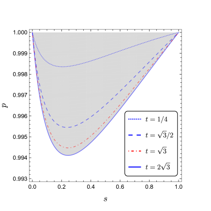
(a) Horodecki’s bound entangled states with white noise

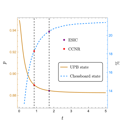
(b) UPB and chessboard states

Figure 1: Entanglement detection criteria. (a) Horodecki’s $3\times 3$ bound entangled states with white noise $\rho_{\mathrm{H}}(s,p)$. (b) UPB bound entangled states with white noise $\rho_{\mathrm{UPB}}(p)$ and $50000$ randomly generated chessboard states $\rho_{\mathrm{CB}}$. Here, we simply take $t_{A}=t_{B}=t$. The larger $t$ detects the more entangled states as shown in (a) and (b), in which $t=\sqrt{3}/2$ and $t=\sqrt{3}$ correspond to CCNR and ESIC criteria, respectively. Diagrams indicate explicitly that the criterion given in Observation 1 outperform CCNR and ESIC criteria under the three typical classes of bound entangled states.

Encouraged by the results in Fig.1, one may naturally ask whether larger $t$ means a more powerful criterion, or, specifically, whether the ESIC criterion is stronger than the CCNR or not, which was conjectured to be true in Ref. [5]. Unfortunately, Eq. 35 can not tell, since the left hand side (lhs) of it contains as well parameters $t_{A}$ and $t_{B}$. Nevertheless, we find this question can be readily addressed under the local filtering transformation (LFT), which preserves the separability of a given state, i.e. $\rho\xmapsto{}\tilde{\rho}=(F_{A}\otimes F_{B})\rho(F_{A}\otimes F_{B})^{\dagger}/\mathrm{Tr}[(F_{A}\otimes F_{B})\rho(F_{A}\otimes F_{B})^{\dagger}]$ with $F_{A/B}$ the arbitrary invertible matrices [51]. LFT transforms the full local rank state into a normal form with maximally mixed subsystems [51, 52]

$$\tilde{\rho}=\frac{1}{d_{A}d_{B}}\mathds{1}\otimes\mathds{1}+\frac{1}{4}\sum_{\mu,\nu}\widetilde{\mathcal{T}}_{\mu\nu}\pi_{\mu}^{A}\otimes\pi_{\nu}^{B}\;.$$ (17)

By dint of quantum states formulated in form of Eq. 17 the bipartite separability problem [52] will be solved. Concretely, we have the following theorem (see Supplemental Material for proof):

Theorem 2.

Let measurement vectors $\boldsymbol{A}$ and $\boldsymbol{B}$ satisfy $\sum_{\mu}t_{\mu}^{A}\vec{a}_{\mu}=\sum_{\mu}t_{\mu}^{B}\vec{b}_{\mu}=0$. If a quantum state $\rho$ is separable, one may find the following relation

$$\mathrm{Tr}\left[\sqrt{\mathcal{A}\widetilde{\mathcal{T}}\mathcal{B}\widetilde{\mathcal{T}}^{\mathrm{T}}}\right]\leq\kappa_{A}\kappa_{B}-\frac{|\vec{t}^{A}||\vec{t}^{B}|}{d_{A}d_{B}}\;,$$ (18)

where $\mathcal{A}=\sum_{\mu}\vec{a}_{\mu}\vec{a}_{\mu}^{\mathrm{T}}$ and $\mathcal{B}=\sum_{\mu}\vec{b}_{\mu}\vec{b}_{\mu}^{\mathrm{T}}$.

As a result of LFT, Theorem 2 formulates a family of even stronger separability criteria than Theorem 1. If $\{\vec{a}_{\mu}\}$ constitutes a regular $(d_{A}^{2}-1)$-simplex, then we readily have $\sum_{\mu}\vec{a}_{\mu}\vec{a}_{\mu}^{\mathrm{T}}=\frac{d_{A}^{2}}{d_{A}^{2}-1}\mathds{1}$ and the following Observation:

Observation 2.

Given measurement vectors $\boldsymbol{A}$ and $\boldsymbol{B}$, let their trace parts satisfy $t_{\mu}^{A}=t_{A},t_{\mu}^{B}=t_{B}$, and traceless parts correspond respectively to a regular simplex. If a quantum state $\rho$ is separable, then in its normal form $\tilde{\rho}$

$$\|\widetilde{\mathcal{T}}\|_{\mathrm{tr}}\leq\kappa(t_{A},t_{B})\;.$$ (19)

Here,

$$\kappa(t_{A},t_{B})=\frac{\sqrt{(d_{A}^{2}-1)(d_{B}^{2}-1)}}{d_{A}d_{B}}\left(\sqrt{t_{A}^{2}+\frac{2d_{A}}{d_{A}+1}}\sqrt{t_{B}^{2}+\frac{2d_{B}}{d_{B}+1}}-|t_{A}t_{B}|\right)\;.$$ (20)

Now that the lhs of Eq. 19 is independent of parameters $t_{A},t_{B}$, one can then strictly compare it with other criteria for different $t_{A}$ and $t_{B}$. Notice that the minimal value of $\kappa(t_{A},t_{B})$, i.e. $\min_{\{t_{A},t_{B}\}}\kappa(t_{A},t_{B})=2\sqrt{(d_{A}-1)(d_{B}-1)/d_{A}d_{B}}$, corresponds to the strongest constraint on separability, which reproduces the Proposition 6 of Ref. [21] when $d_{A}=d_{B}$. Furthermore, the CCNR and ESIC criteria will reexhibit respectively while we take $\kappa(t_{A},t_{B})=2-2/\sqrt{d_{A}d_{B}}$ and $4-2\sqrt{(d_{A}+1)(d_{B}+1)/d_{A}d_{B}}$, which also implies that in normal form the ESIC criterion is stronger than CCNR and they coincide as $d_{A}=d_{B}$.

Relations to entanglement witness

An entanglement witness is a Hermitian operator which has nonnegative expectation values for all separable states and negative one for some entangled states [7, 53]. Entanglement witness provides an experimental friendly tool to analyse entanglement [3]. To this end, we reformulate the Theorem 1 in terms of entanglement witness. Given a correlation matrix $\mathcal{C}$ for measurement vectors $\boldsymbol{A},\boldsymbol{B}$, we readily find

$$\|\mathcal{C}\|_{\mathrm{tr}}=\sum_{\mu=1}^{r}\braket{A^{\prime}_{\mu}\otimes B^{\prime}_{\mu}}\;.$$ (21)

Here, $A^{\prime}_{\mu}=\sum_{\nu}P_{\nu\mu}A_{\nu}$, $B^{\prime}_{\mu}=\sum_{\nu}Q_{\nu\mu}B_{\nu}$ and $P,Q$ achieve a singular value decomposition of $\mathcal{C}$, i.e. $\mathcal{C}=P\Sigma Q^{\mathrm{T}}$, where $P,Q$ are orthogonal matrices, $\Sigma=\operatorname{diag}\{\sigma_{1},\cdots,\sigma_{r},0,\cdots,0\}$ with singular values $\sigma_{k}$ and $\operatorname{rank}(\mathcal{C})=r$ [54]. Thus, one may immediately get an inequality of correlation function similar to CHSH inequality Eq. 4 for separable state

$$\sum_{\mu=1}^{r}\braket{A^{\prime}_{\mu}\otimes B^{\prime}_{\mu}}\leq\kappa\;,$$ (22)

where $\kappa=\kappa_{A}\kappa_{B}$. Obviously, Eq. 22 can be reformulated as the following entanglement witness

$$\mathcal{W}=\kappa\mathds{1}\otimes\mathds{1}-\sum_{\mu=1}^{r}A^{\prime}_{\mu}\otimes B^{\prime}_{\mu}\;.$$ (23)

This means that based upon the extended Bloch space, entanglement witness will be simply generated for generic observables.

Further extensions

Through the construction of a measurement-induced Bloch space, we have established a general condition for separability which arises from the constraint of the length of the MIBVs. However, not only the moduli of MIBVs but also their directions suffice a constraint. As an illustration, we consider the measurement vector $\boldsymbol{A}=\boldsymbol{B}=\vec{\pi}$, in which case the measurement-induced Bloch space reduces to the familiar Bloch space. Then the angel $\theta$ between any two Bloch vectors of pure states satisfies $-\frac{1}{d-1}\leq\cos\theta\leq 1$ [55, 35]. Given a $d\times d$ bipartite state, if it is separable, i.e. $\mathcal{T}=\sum_{i}p_{i}\vec{r}_{i}\vec{s}_{i}^{\mathrm{T}}$ with $\vec{r}_{i}$ and $\vec{s}_{i}$ being the Bloch vectors, we find the criterion

$$-\frac{2}{d}\leq\mathrm{Tr}[\mathcal{T}]\leq\frac{2(d-1)}{d}$$ (24)

exists, otherwise the entanglement survives. We notice $\mathrm{Tr}[\mathcal{T}]=\sum_{\mu=1}^{d^{2}-1}\braket{\pi_{\mu}\otimes\pi_{\mu}}$, so Eq. 24 yields the entanglement witness $\mathcal{W}=\frac{2}{d}\mathds{1}\otimes\mathds{1}+\sum_{\mu}\pi_{\mu}\otimes\pi_{\mu}$. Considering arbitrary dimensional Werner states [47, 56]

$$\rho_{\mathrm{W}}=\frac{1}{d^{2}}\mathds{1}\otimes\mathds{1}+\frac{1}{4}\sum_{\mu=1}^{d^{2}-1}\frac{2(d\phi-1)}{d(d^{2}-1)}\pi_{\mu}\otimes\pi_{\mu}\;,\;\forall\phi\in[-1,1]\;,$$

which is separable if and only if $\phi\geq 0$ [47]. An simple calculation shows that Eq. 24 is a necessary and sufficient condition taking effect in full parameter space $\phi\in[-1,0)$ , while CCNR and ESIC criteria are valid merely in $\phi\in[-1,-\frac{d-2}{d}]$. With the growth of dimensionality, the entanglement detectable intervals of CCNR and ESIC criteria tend to none. This example tells that we can establish more powerful separability condition than existing ones by only employing the inherent constraints in Bloch space. On this account, we are tempting to conclude that the inherent constraints in Bloch space may address a lot of the separability issues.

Concluding remarks

In the framework of measurement-induced Bloch space, by dint of a novel scheme we obtain a family of stronger separability criteria for entangled system. These criteria encompass many of the well-known existing results, meanwhile explicitly show why they work, i.e. the correlation matrix of a separable state is constrained by the measurement-induced Bloch space. Moreover, the new criteria can be transformed into entanglement witness operators, which makes the construction of entanglement witness from generic observables even transparent. Finally, It is noteworthy that the method developed in this work is in principle extendable to the multipartite systems by introducing the corresponding multipartite correlation tensors, though some tedious work needs to be done.

Supplemental Material

Here we elaborate and derive in detail the main results discussed in the main text.

The proof of Theorem 1

Given arbitrary measurement vectors $\boldsymbol{A}$ and $\boldsymbol{B}$ with with $\sum_{\mu}t_{\mu}^{A}\vec{a}_{\mu}=\sum_{\mu}t_{\mu}^{B}\vec{b}_{\mu}=0$, the correlation matrices of the separable states can be expressed as

$$\mathcal{C}=\sum_{i}p_{i}(\vec{t}\,^{A}/d_{A}+\vec{\alpha}_{i})(\vec{t}\,^{B}/d_{B}+\vec{\beta}_{i})^{\mathrm{T}}\;.$$ (25)

Here, $\vec{\alpha}_{i}$ and $\vec{\beta}_{i}$ are the generalized Bloch vectors associated with $\boldsymbol{A}$ and $\boldsymbol{B}$ as defined in the main text. Employing the convexity property of trace norm $\|X\|_{\operatorname{tr}}=\mathrm{Tr}\left[\sqrt{X^{\dagger}X}\right]$, we have

$$\|\mathcal{C}\|_{\mathrm{tr}} \leq\sum_{i}p_{i}|\vec{t}\,^{A}/d_{A}+\vec{\alpha}_{i}||\vec{t}\,^{B}/d_{B}+\vec{\beta}_{i}|$$ (26)

$$=\sqrt{(\vec{t}\,^{A})^{2}/d_{A}^{2}+\vec{\alpha}_{i}^{2}}\sqrt{(\vec{t}\,^{B})^{2}/d_{B}^{2}+\vec{\beta}_{i}^{2}}\;.$$ (27)

Here, we make use of $\sum_{\mu}t_{\mu}^{A}\vec{a}_{\mu}=\sum_{\mu}t_{\mu}^{B}\vec{b}_{\mu}=0$ and $|\cdot|$ denotes Euclidean norm of a real vector. So, the correlation matrices of the separable states are limited by the size of the measurement-induced Bloch space (MIBS). Next, we prove that the MIBS is bounded and its boundary can be obtained simply.

Given a measurement vector $\boldsymbol{A}$, quantum states can be transformed into the measurement-induced Bloch vector (MIBVs) which constitute the MIBS. It is found that the MIBVs satisfy the following equation [1]

$$\vec{\alpha}^{\mathrm{T}}\Omega^{-}\vec{\alpha}=\mathrm{Tr}[\rho^{2}]-\frac{1}{d}\;.$$ (28)

Here, $\Omega_{\mu\nu}\equiv\mathrm{Tr}[\bar{A}_{\mu}\bar{A}_{\nu}]=2\vec{a}_{\mu}\cdot\vec{a}_{\nu}$ and $\Omega^{-}$ denotes the Moore-Penrose inverse of $\Omega$. Eq. 28 is an ellipsoid equation, which characterizes the MIBS, that is,

$$\mathcal{B}(\boldsymbol{A})=\left\{\vec{\alpha}\Big{|}\sqrt{\frac{d}{d\mathrm{Tr}[\rho^{2}]-1}}\vec{\alpha}^{\mathrm{T}}\Omega^{-}\sqrt{\frac{d}{d\mathrm{Tr}[\rho^{2}]-1}}\vec{\alpha}\leq 1\right\}\;.$$ (29)

Matrix $\Omega$ completely depicts the properties of the ellipsoid defined by Eq. 29, such as the lengths of the semi-axes are given by $\sqrt{\frac{(d\mathrm{Tr}[\rho^{2}]-1)\lambda_{i}}{d}}$, with $\lambda_{i}$ being the eigenvalues of $\Omega$; the eigenvectors of $\Omega$ determines the directions of the semi-axes [2]. Obviously, Bloch space is a special case of $\boldsymbol{A}=\vec{\pi}$. So, for arbitrary measurement vector $\boldsymbol{A}$, we have

$$|\vec{\alpha}|^{2}\leq\frac{d-1}{d}\lambda_{\max}(\Omega)\;,$$ (30)

where $\lambda_{\max}(X)$ is the maximal eigenvalue of matrix $X$. Finally, we prove

$$\|\mathcal{C}\|_{\operatorname{tr}}\leq\kappa_{A}\kappa_{B}\;.$$ (31)

Here, $\kappa_{A}=\sqrt{(\vec{t}\,^{A})^{2}/d_{A}^{2}+\frac{d_{A}-1}{d_{A}}\lambda_{\max}(\Omega_{A})}$ and $(\Omega_{A})_{\mu\nu}=2\vec{a}_{\mu}\cdot\vec{a}_{\nu}$, similarly for $\kappa_{B}$.

The proof of Observation 1

If $\boldsymbol{A}$ has the same trace and the traceless part corresponds to a regular simplex, namely

$$M_{A}=\left(\begin{matrix}\frac{t_{A}}{\sqrt{2d_{A}}}&\frac{t_{A}}{\sqrt{2d_{A}}}&\cdots&\frac{t_{A}}{\sqrt{2d_{A}}}\\ \vec{a}_{1}&\vec{a}_{2}&\cdots&\vec{a}_{d_{A}^{2}}\end{matrix}\right)\;,$$ (32)

where $\{\vec{a}_{\mu}\}$ constitutes a regular $(d_{A}^{2}-1)$-simplex, i.e. $\left\{\vec{a}_{\mu}\Big{|}\vec{a}_{\mu}\cdot\vec{a}_{\nu}=\frac{d_{A}^{2}\delta_{\mu\nu}-1}{d_{A}^{2}-1}\right\},\mu,\nu=1,\cdots,d_{A}^{2}$, then we have $(\Omega_{A})_{\mu\nu}=2\vec{a}_{\mu}\cdot\vec{a}_{\nu}=2\frac{d_{A}^{2}\delta_{\mu\nu}-1}{d_{A}^{2}-1}$, whose matrix form is

$$\Omega_{A}=\frac{2}{d_{A}^{2}-1}\left(d_{A}^{2}\mathds{1}-J_{d_{A}^{2}}\right)\;,$$ (33)

where, $J_{d_{A}^{2}}$ is a $d_{A}^{2}$-dimensional all-ones matrix all whose elements are equal to one. On account of $J_{d_{A}^{2}}^{2}=d_{A}^{2}J_{d_{A}^{2}}$, it is readily to find eigenvalues of $J_{d_{A}^{2}}$, i.e. $d_{A}^{2}$ and $0$ ($d_{A}^{2}-1$-fold degeneracy). Hence, we have $\lambda_{\max}(\Omega_{A})=\frac{2d_{A}^{2}}{d_{A}^{2}-1}$, and

$$\kappa_{A}=\sqrt{t_{A}^{2}+\frac{2d_{A}}{d_{A}+1}}\;,$$ (34)

similarly for $\kappa_{B}$. So, for the separable state, we have

$$\|\mathcal{C}\|_{\mathrm{tr}}\leq\sqrt{t_{A}^{2}+\frac{2d_{A}}{d_{A}+1}}\sqrt{t_{B}^{2}+\frac{2d_{B}}{d_{B}+1}}\;,$$ (35)

Here, parameters $t_{A}$ and $t_{B}$ can be arbitrary real numbers. And next, we prove that, when $t_{X}=\sqrt{\frac{2d_{X}}{d_{X}^{2}-1}}$ and $t_{X}=\sqrt{\frac{2d_{X}}{d_{X}-1}}$ for $X=A,B$, Eq. 35 reproduces CCNR and ESIC (entanglement criterion via SIC-POVM) criteria, respectively. Firstly, we review the CCNR criterion. A bipartite state can be expressed as

$$\rho=\frac{1}{4}\sum_{\mu,\nu}\chi_{\mu\nu}\Pi_{\mu}^{A}\otimes\Pi_{\nu}^{B}\;.$$ (36)

Here, $\Pi_{0}^{X}=\sqrt{\frac{2}{d_{X}}}\mathds{1}$ and $\{\Pi_{\mu}^{X}=\pi_{\mu}^{X}\}_{\mu=1}^{d_{X}^{2}-1}$ is generators of $\mathfrak{su}(d_{X})$ Lie algebra for $X=A,B$; $\{\Pi_{\mu}^{X}\}_{\mu=0}^{d_{X}^{2}-1}$ satisfies the orthogonal relation $\mathrm{Tr}[\Pi_{\mu}^{X}\Pi_{\nu}^{X}]=2\delta_{\mu\nu}$. Making use of the Schmidt decomposition in operator space, we have

$$\rho=\frac{1}{4}\sum_{\mu,\nu}\chi_{\mu\nu}\Pi_{\mu}^{A}\otimes\Pi_{\nu}^{B}=\sum_{k}\sigma_{k}\widetilde{\Pi}_{k}^{A}\otimes\widetilde{\Pi}_{k}^{B}\;.$$ (37)

Here, $\sum_{k}\sigma_{k}=\frac{1}{2}\|\chi\|_{\mathrm{tr}}$ and $\{\widetilde{\Pi}_{k}^{A}\}$ and $\{\widetilde{\Pi}_{k}^{B}\}$ form orthonormal bases of the operator space. CCNR criterion says that, if $\rho$ is separable, then we have $\sum_{k}\sigma_{k}\leq 1$ [3, 4], that is, $\|\chi\|_{\mathrm{tr}}\leq 2$. If $t_{X}=\sqrt{\frac{2d_{X}}{d_{X}^{2}-1}}$ for $X=A,B$, then we have

$$M_{A}^{\mathrm{T}}M_{A} =\left(\begin{matrix}\frac{1}{\sqrt{d_{A}^{2}-1}}&\vec{a}_{1}\\ \frac{1}{\sqrt{d_{A}^{2}-1}}&\vec{a}_{2}\\ \vdots&\vdots\\ \frac{1}{\sqrt{d_{A}^{2}-1}}&\vec{a}_{d_{A}^{2}}\end{matrix}\right)\left(\begin{matrix}\frac{1}{\sqrt{d_{A}^{2}-1}}&\frac{1}{\sqrt{d_{A}^{2}-1}}&\cdots&\frac{1}{\sqrt{d_{A}^{2}-1}}\\ \vec{a}_{1}&\vec{a}_{2}&\cdots&\vec{a}_{d_{A}^{2}}\end{matrix}\right)=\frac{d_{A}^{2}}{d_{A}^{2}-1}\mathds{1}\;.$$ (38)

Here, $\vec{a}_{\mu}\cdot\vec{a}_{\nu}=\frac{d_{A}^{2}\delta_{\mu\nu}-1}{d_{A}^{2}-1}$ has been employed. Similarly, we have $M_{A}^{\mathrm{T}}M_{A}=\frac{d_{B}^{2}}{d_{B}^{2}-1}\mathds{1}$. So, if $t_{X}=\sqrt{\frac{2d_{X}}{d_{X}^{2}-1}}$ for $X=A,B$, Eq. 35 gives $\|\mathcal{C}\|_{\mathrm{tr}}=\|M_{A}^{\mathrm{T}}\chi M_{B}\|_{\mathrm{tr}}=\frac{d_{A}d_{B}}{\sqrt{(d_{A}^{2}-1)(d_{B}^{2}-1)}}\|\chi\|_{\mathrm{tr}}\leq\frac{2d_{A}d_{B}}{\sqrt{(d_{A}^{2}-1)(d_{B}^{2}-1)}}$, that is, $\|\chi\|_{\mathrm{tr}}\leq 2$.

And then, the ESIC criteria says that if $\rho$ is separable, then the correlation matrix of the normalized SIC-POVM $\{E_{\mu}^{A}\}$ and $\{E_{\mu}^{B}\}$ satisfies [5]

$$\|\mathcal{P}\|_{\mathrm{tr}}\leq 1\;,$$ (39)

where $\mathcal{P}_{\mu\nu}=\braket{E_{\mu}^{A}\otimes E_{\nu}^{B}}$, $E_{\mu}^{X}\geq 0$ and $\mathrm{Tr}[E_{\mu}^{X}E_{\nu}^{X}]=\frac{d_{X}\delta_{\mu\nu}+1}{2d_{X}},\mu,\nu=1,2,\cdots,d_{X}^{2}$ for $X=A,B$. It is noteworthy that the original assumption about the existence of SIC-POVM is not essential as shown in [6]. In fact, we can obtain ESIC criterion for arbitrary measurement vector $\boldsymbol{A}$ satisfying $\mathrm{Tr}[A_{\mu}A_{\nu}]=\alpha\frac{d\delta_{\mu\nu}+1}{2d},\mu,\nu=1,2,\cdots,d^{2}$ with nonzero real parameter $\alpha$. If $t_{X}=\sqrt{\frac{2d_{X}}{d_{X}-1}}$ for $X=A,B$, we have $\mathrm{Tr}[A_{\mu}A_{\nu}]=\frac{t_{A}^{2}}{d}+2\vec{a}_{\mu}\cdot\vec{a}_{\nu}=\frac{(2d_{A})^{2}}{d_{A}^{2}-1}\frac{d_{A}\delta_{\mu\nu}+1}{2d_{A}}$ and Eq. 35 gives

$$\|\mathcal{C}\|_{\mathrm{tr}}\leq\frac{4d_{A}d_{B}}{\sqrt{(d_{A}^{2}-1)(d_{B}^{2}-1)}}\;,$$ (40)

which reproduces the ESIC criterion due to $\braket{A_{\mu}\otimes B_{\nu}}=\frac{4d_{A}d_{B}}{\sqrt{(d_{A}^{2}-1)(d_{B}^{2}-1)}}\braket{E_{\mu}^{A}\otimes E_{\nu}^{B}}$.

The vertex coordinates for regular simplex

There are many methods to generate the vertex coordinates for regular simplex, where we give a simple scheme for the reader’s convenience. Given the following $n$-dimensional unit vectors

$$\vec{e}_{k}=(b_{1},b_{2},\cdots,b_{k-1},a_{k},0,\cdots,0)\;,$$ (41)

and

$$a_{k}=\frac{\sqrt{(n+1)(n-k+1)}}{\sqrt{n(n-k+2)}},b_{k}=-\frac{\sqrt{\ n+1}}{\sqrt{n(n-k+1)(n-k+2)}},k=1,2,\cdots,n+1,$$ (42)

then $\{\vec{e}_{1},\vec{e}_{2}\cdots,\vec{e}_{n+1}\}$ constitutes a $n$-dimensional regular simplex. The following is an example for $n=8$,

$$\left(\begin{array}[]{ccccccccc}1&-\frac{1}{8}&-\frac{1}{8}&-\frac{1}{8}&-\frac{1}{8}&-\frac{1}{8}&-\frac{1}{8}&-\frac{1}{8}&-\frac{1}{8}\\ 0&\frac{3\sqrt{7}}{8}&-\frac{3}{8\sqrt{7}}&-\frac{3}{8\sqrt{7}}&-\frac{3}{8\sqrt{7}}&-\frac{3}{8\sqrt{7}}&-\frac{3}{8\sqrt{7}}&-\frac{3}{8\sqrt{7}}&-\frac{3}{8\sqrt{7}}\\ 0&0&\frac{3}{2}\sqrt{\frac{3}{7}}&-\frac{1}{4}\sqrt{\frac{3}{7}}&-\frac{1}{4}\sqrt{\frac{3}{7}}&-\frac{1}{4}\sqrt{\frac{3}{7}}&-\frac{1}{4}\sqrt{\frac{3}{7}}&-\frac{1}{4}\sqrt{\frac{3}{7}}&-\frac{1}{4}\sqrt{\frac{3}{7}}\\ 0&0&0&\frac{\sqrt{15}}{4}&-\frac{1}{4}\sqrt{\frac{3}{5}}&-\frac{1}{4}\sqrt{\frac{3}{5}}&-\frac{1}{4}\sqrt{\frac{3}{5}}&-\frac{1}{4}\sqrt{\frac{3}{5}}&-\frac{1}{4}\sqrt{\frac{3}{5}}\\ 0&0&0&0&\frac{3}{\sqrt{10}}&-\frac{3}{4\sqrt{10}}&-\frac{3}{4\sqrt{10}}&-\frac{3}{4\sqrt{10}}&-\frac{3}{4\sqrt{10}}\\ 0&0&0&0&0&\frac{3}{4}\sqrt{\frac{3}{2}}&-\frac{1}{4}\sqrt{\frac{3}{2}}&-\frac{1}{4}\sqrt{\frac{3}{2}}&-\frac{1}{4}\sqrt{\frac{3}{2}}\\ 0&0&0&0&0&0&\frac{\sqrt{3}}{2}&-\frac{\sqrt{3}}{4}&-\frac{\sqrt{3}}{4}\\ 0&0&0&0&0&0&0&\frac{3}{4}&-\frac{3}{4}\\ \end{array}\right)\;.$$ (51)

Bound entangled states

Horodecki’s bound entangled states with white noise:

$$\rho_{\mathrm{H}}(s,p)=p\rho_{\mathrm{H}}(s)+(1-p)\mathds{1}/9\;,\;0\leq p\leq 1\;.$$ (52)

Here, $\rho_{\mathrm{H}}(t)$ is $3\times 3$ Horodecki’s bound entangled states [7], i.e.

$$\rho_{\mathrm{H}}(s)=\frac{1}{8s+1}\left(\begin{matrix}s&0&0&0&s&0&0&0&s\\ 0&s&0&0&0&0&0&0&0\\ 0&0&s&0&0&0&0&0&0\\ 0&0&0&s&0&0&0&0&0\\ s&0&0&0&s&0&0&0&s\\ 0&0&0&0&0&s&0&0&0\\ 0&0&0&0&0&0&\frac{1}{2}(1+s)&0&\frac{1}{2}\sqrt{1-s^{2}}\\ 0&0&0&0&0&0&0&s&0\\ s&0&0&0&s&0&\frac{1}{2}\sqrt{1-s^{2}}&0&\frac{1}{2}(1+s)\end{matrix}\right)\;.$$ (53)

Unextendible product bases (UPB) bound entangled states:

$$\rho_{\mathrm{UPB}}(p)=p\rho_{\mathrm{UPB}}+(1-p)\mathds{1}/9\;,\;0\leq p\leq 1\;.$$ (54)

Here, $\rho_{\mathrm{UPB}}$ is bound entangled state constructed by UPB [8], i.e.

$$\rho_{\mathrm{UPB}}=\frac{1}{4}\left(\mathds{1}-\sum_{i=0}^{4}\ket{\psi_{i}}\bra{\psi_{i}}\right)\;,$$ (55)

and

$$\ket{\psi_{0}}=\frac{1}{\sqrt{2}}\ket{0}\left(\ket{0}-\ket{1}\right)\;,\;\ket{\psi_{1}}=\frac{1}{\sqrt{2}}(\ket{0}-\ket{1})\ket{2}\;,$$ (56)

$$\ket{\psi_{2}}=\frac{1}{\sqrt{2}}\ket{2}(\ket{1}-\ket{2})\;,\;\ket{\psi_{3}}=\frac{1}{\sqrt{2}}(\ket{1}-\ket{2})\ket{0}\;,$$

$$\ket{\psi_{4}}=\frac{1}{3}(\ket{0}+\ket{1}+\ket{2})(\ket{0}+\ket{1}+\ket{2})\;.$$

Chessboard states [9]:

$$\rho_{\mathrm{CB}}=\mathcal{N}\sum_{i=1}^{4}\ket{V_{i}}\bra{V_{i}}\;.$$ (57)

Here, $\mathcal{N}=1/\sum_{i}\braket{V_{i}}{V_{i}}$ is normalization constant and the unnormalized vectors $\ket{V_{i}}$ are

$$\ket{V_{1}}=\ket{m,0,ac/n;0,n,0;0,0,0}\;,$$

$$\ket{V_{2}}=\ket{0,a,0;b,0,c;0,0,0}\;,$$

$$\ket{V_{3}}=\ket{n,0,0;0,-m,0;ad/m,0,0}\;,$$

$$\ket{V_{4}}=\ket{0,b,0;-a,0,0;0,d,0}\;.$$ (58)

Chessboard states contain six real parameters $m,n,a,b,c,d$. In the main text, we test Observation 1 by randomly generated $50000$ chessboard states, where the six parameters are drawn independently from the standard normal distribution.

The proof of Theorem 2

By virtue of Bloch representation, the correlation matrix can be written as $\mathcal{C}=M_{A}^{\mathrm{T}}\chi M_{B}$, so we have

$$\|\mathcal{C}\|_{\mathrm{tr}}=\mathrm{Tr}\left[\sqrt{\mathcal{C}^{\mathrm{T}}\mathcal{C}}\right]=\mathrm{Tr}\left[\sqrt{M_{B}M_{B}^{\mathrm{T}}\chi^{\mathrm{T}}M_{A}M_{A}^{\mathrm{T}}\chi}\right]\;.$$ (59)

Given arbitrary measurement vectors $\boldsymbol{A}$ and $\boldsymbol{B}$ with $\sum_{\mu}t_{\mu}^{A}\vec{a}_{\mu}=\sum_{\mu}t_{\mu}^{B}\vec{b}_{\mu}=0$, we have

$$M_{A}=\left(\begin{matrix}\frac{t_{1}^{A}}{\sqrt{2d_{A}}}&\frac{t_{2}^{A}}{\sqrt{2d_{A}}}&\cdots\\ \vec{a}_{1}&\vec{a}_{2}&\cdots\end{matrix}\right)\;,\;M_{B}=\left(\begin{matrix}\frac{t_{1}^{B}}{\sqrt{2d_{B}}}&\frac{t_{2}^{B}}{\sqrt{2d_{B}}}&\cdots\\ \vec{b}_{1}&\vec{b}_{2}&\cdots\end{matrix}\right)\;,$$ (60)

and

$$M_{A}M_{A}^{\mathrm{T}}=\left(\begin{matrix}\frac{(\vec{t}^{A})^{2}}{2d_{A}}&0\\ 0&\mathcal{A}\end{matrix}\right)=\frac{(\vec{t}^{A})^{2}}{2d_{A}}\oplus\mathcal{A}\;,$$ (61)

where $\mathcal{A}=\sum_{\mu}\vec{a}_{\mu}\vec{a}_{\mu}^{\mathrm{T}}$. Similarly, we have $M_{B}M_{B}^{\mathrm{T}}=\frac{(\vec{t}^{B})^{2}}{2d_{B}}\oplus\mathcal{B}$ and $\mathcal{B}=\sum_{\mu}\vec{b}_{\mu}\vec{b}_{\mu}^{\mathrm{T}}$. For the normal form states, we have $\chi=\frac{2}{\sqrt{d_{A}d_{B}}}\oplus\widetilde{\mathcal{T}}$. And then,

$$\|\mathcal{C}\|_{\mathrm{tr}} =\mathrm{Tr}\left[\sqrt{M_{B}M_{B}^{\mathrm{T}}\chi^{\mathrm{T}}M_{A}M_{A}^{\mathrm{T}}\chi}\right]$$ (62)

$$=\mathrm{Tr}\left[\sqrt{\frac{(\vec{t}^{A})^{2}(\vec{t}^{B})^{2}}{d_{A}^{2}d_{B}^{2}}\oplus\mathcal{B}\widetilde{\mathcal{T}}^{\mathrm{T}}\mathcal{A}\widetilde{\mathcal{T}}}\right]$$ (63)

$$=\frac{|\vec{t}^{A}||\vec{t}^{B}|}{d_{A}d_{B}}+\mathrm{Tr}\left[\sqrt{\mathcal{A}\widetilde{\mathcal{T}}\mathcal{B}\widetilde{\mathcal{T}}^{\mathrm{T}}}\right]\;.$$ (64)

So, if a quantum state $\rho$ is separable, then we have in its normal form $\tilde{\rho}$

$$\mathrm{Tr}\left[\sqrt{\mathcal{A}\widetilde{\mathcal{T}}\mathcal{B}\widetilde{\mathcal{T}}^{\mathrm{T}}}\right]\leq\kappa_{A}\kappa_{B}-\frac{|\vec{t}^{A}||\vec{t}^{B}|}{d_{A}d_{B}}\;.$$ (65)

References

• [1] V. Vedral, Quantum entanglement, Nat. Phys. 10, 256–258 (2014).
• [2] R. Horodecki, P. Horodecki, M. Horodecki, and K. Horodecki, Quantum entanglement, Rev. Mod. Phys. 81, 865 (2009).
• [3] O. Gühne and G. Tóth, Entanglement detection, Phys. Rep. 474, 1–75 (2009).
• [4] L. Gurvits, Classical complexity and quantum entanglement, J Comput Syst Sci 69, 448–484 (2004).
• [5] M. Horodecki, P. Horodecki, and R. Horodecki, Separability of mixed states: Necessary and sufficient conditions, Phys. Lett. A 223, 1–8 (1996).
• [6] A. Peres, Separability Criterion for Density Matrices, Phys. Rev. Lett. 77, 1413 (1996).
• [7] M. Horodecki, P. Horodecki, and R. Horodecki, Separability of n-particle mixed states: necessary and sufficient conditions in terms of linear maps, Phys. Lett. A 283, 1–7 (2001).
• [8] O. Rudolph, A separability criterion for density operators, J. Phys. A 33, 3951–3955 (2000).
• [9] K. Chen and L.-A. Wu, A matrix realignment method for recognizing entanglement, Quantum Inf. Comput. 3, 193–202 (2003).
• [10] O. Rudolph, Further results on the cross norm criterion for separability, Quantum Inf. Process. 4, 219–239 (2005).
• [11] J. I. de Vicente, Separability criteria based on the Bloch representation of density matrices, Quantum Inf. Comput. 7, 624 (2007).
• [12] J. I. de Vicente, Further results on entanglement detection and quantification from the correlation matrix criterion, J. Phys. A: Math. Theor. 41, 065309 (2008).
• [13] J.-L. Li and C.-F. Qiao, A Necessary and Sufficient Criterion for the Separability of Quantum State, Sci. Rep. 8, 1442 (2018).
• [14] J. Shang, A. Asadian, H. Zhu, and O. Gühne, Enhanced entanglement criterion via symmetric informationally complete measurements, Phys. Rev. A 98, 022309 (2018).
• [15] L. M. Duan, G. Giedke, J. I. Cirac, and P. Zoller, Inseparability criterion for continuous variable systems, Phys. Rev. Lett. 84, 2722 (2000).
• [16] H. F. Hofmann and S. Takeuchi, Violation of local uncertainty relations as a signature of entanglement, Phys. Rev. A 68, 032103 (2003).
• [17] O. Gühne, Characterizing entanglement via uncertainty relations, Phys. Rev. Lett. 92, 117903 (2004).
• [18] C. J. Zhang, Y. S. Zhang, S. Zhang, and G. C. Guo, Optimal entanglement witnesses based on local orthogonal observables, Phys. Rev. A 76, 012334 (2007).
• [19] C. J. Zhang, H. Nha, Y. S. Zhang, and G. C. Guo, Entanglement detection via tighter local uncertainty relations, Phys. Rev. A 81, 012324 (2010).
• [20] R. Schwonnek, L. Dammeier, and R. F. Werner, State-Independent Uncertainty Relations and Entanglement Detection in Noisy Systems, Phys. Rev. Lett. 119, 170404 (2017).
• [21] O. Gühne, P. Hyllus, O. Gittsovich, and J. Eisert, Covariance matrices and the separability problem, Phys. Rev. Lett. 99, 130504 (2007).
• [22] O. Gittsovich, O. Gühne, P. Hyllus, and J. Eisert, Unifying several separability conditions using the covariance matrix criterion, Phys. Rev. A 78, 052319 (2008).
• [23] P. Hyllus, W. Laskowski, R. Krischek, C. Schwemmer, W. Wieczorek, H. Weinfurter, L. Pezze, and A. Smerzi, Fisher information and multiparticle entanglement, Phys. Rev. A 85, 022321 (2012).
• [24] N. Li and S. L. Luo, Entanglement detection via quantum Fisher information, Phys. Rev. A 88, 014301 (2013).
• [25] Z. Ren, W. Li, A. Smerzi, and M. Gessner, Metrological Detection of Multipartite Entanglement from Young Diagrams, Phys. Rev. Lett. 126, 080502 (2021).
• [26] E. Shchukin and W. Vogel, Inseparability criteria for continuous bipartite quantum states, Phys. Rev. Lett. 95, 230502 (2005).
• [27] A. Elben, R. Kueng, H. R. Huang, R. van Bijnen, C. Kokail, M. Dalmonte, P. Calabrese, B. Kraus, J. Preskill, P. Zoller, and B. Vermersch, Mixed-State Entanglement from Local Randomized Measurements, Phys. Rev. Lett. 125, 200501 (2020).
• [28] A. Neven, J. Carrasco, V. Vitale, C. Kokail, A. Elben, M. Dalmonte, P. Calabrese, P. Zoller, B. Vermersch, R. Kueng, and B. Kraus, Symmetry-resolved entanglement detection using partial transpose moments, NPJ Quantum Inf. 7, 1–12 (2021).
• [29] X. D. Yu, S. Imai, and O. Guhne, Optimal Entanglement Certification from Moments of the Partial Transpose, Phys. Rev. Lett. 127, 060504 (2021).
• [30] U. Fano, Description of States in Quantum Mechanics by Density Matrix and Operator Techniques, Rev. Mod. Phys. 29, 74 (1957).
• [31] J. E. Harriman, Geometry of density matrices. I. Definitions, $N$ matrices and $1$ matrices, Phys. Rev. A 17, 1249 (1978).
• [32] F. T. Hioe and J. H. Eberly, N-Level Coherence Vector and Higher Conservation Laws in Quantum Optics and Quantum Mechanics, Phys. Rev. Lett. 47, 838 (1981).
• [33] M. S. Byrd and N. Khaneja, Characterization of the positivity of the density matrix in terms of the coherence vector representation, Phys. Rev. A 68, 062322 (2003).
• [34] J. L. Li and C. F. Qiao, Reformulating the Quantum Uncertainty Relation, Scientific Reports 5, 12708 (2015).
• [35] G. Kimura, The Bloch vector for N-level systems, Phys. Lett. A 314, 339–349 (2003).
• [36] A. Einstein, B. Podolsky, and N. Rosen, Can Quantum-Mechanical Description of Physical Reality Be Considered Complete?, Phys. Rev. 47, 777 (1935).
• [37] E. Schrödinger, Discussion of Probability Relations between Separated Systems, Math. Proc. Cambridge Philos. Soc. 31, 555–563 (1935).
• [38] J. S. Bell, On the Einstein Podolsky Rosen paradox, Physics Physique Fizika 1, 195 (1964).
• [39] J. F. Clauser, M. A. Horne, A. Shimony, and R. A. Holt, Proposed Experiment to Test Local Hidden-Variable Theories, Phys. Rev. Lett. 23, 880 (1969).
• [40] S. J. Freedman and J. F. Clauser, Experimental Test of Local Hidden-Variable Theories, Phys. Rev. Lett. 28, 938 (1972).
• [41] A. Aspect, P. Grangier, and G. Roger, Experimental Realization of Einstein-Podolsky-Rosen-Bohm Gedankenexperiment: A New Violation of Bell’s Inequalities, Phys. Rev. Lett. 49, 91 (1982).
• [42] A. Aspect, J. Dalibard, and G. Roger, Experimental Test of Bell’s Inequalities Using Time- Varying Analyzers, Phys. Rev. Lett. 49, 1804 (1982).
• [43] M. A. Rowe, D. Kielpinski, V. Meyer, C. A. Sackett, W. M. Itano, C. Monroe, and D. J. Wineland, Experimental violation of a Bell’s inequality with efficient detection, Nature 409, 791–794 (2001).
• [44] B. Hensen, H. Bernien, A. E. Dreau, A. Reiserer, N. Kalb, M. S. Blok, J. Ruitenberg, R. F. Vermeulen, R. N. Schouten, C. Abellan, W. Amaya, V. Pruneri, M. W. Mitchell, M. Markham, D. J. Twitchen, D. Elkouss, S. Wehner, T. H. Taminiau, and R. Hanson, Loophole-free Bell inequality violation using electron spins separated by 1.3 kilometres, Nature 526, 682–686 (2015).
• [45] J. Handsteiner, A. S. Friedman, D. Rauch, J. Gallicchio, B. Liu, H. Hosp, J. Kofler, D. Bricher, M. Fink, C. Leung, A. Mark, H. T. Nguyen, I. Sanders, F. Steinlechner, R. Ursin, S. Wengerowsky, A. H. Guth, D. I. Kaiser, T. Scheidl, and A. Zeilinger, Cosmic Bell Test: Measurement Settings from Milky Way Stars, Phys. Rev. Lett. 118, 060401 (2017).
• [46] B. I. G. B. T. Collaboration, Challenging local realism with human choices, Nature 557, 212–216 (2018).
• [47] R. F. Werner, Quantum states with Einstein-Podolsky-Rosen correlations admitting a hidden-variable model, Phys. Rev. A 40, 4277 (1989).
• [48] M.-C. Yang and C.-F. Qiao, Certainty and Uncertainty Relations via Measurement Orbits Submitted.
• [49] G. Sarbicki, G. Scala, and D. Chruściński, Family of multipartite separability criteria based on a correlation tensor, Phys. Rev. A 101, 012341 (2020).
• [50] O. Rudolph, Some properties of the computable cross-norm criterion for separability, Phys. Rev. A 67, 032312 (2003).
• [51] F. Verstraete, J. Dehaene, and B. D. Moor, Normal forms and entanglement measures for multipartite quantum states, Phys. Rev. A 68, 012103 (2003).
• [52] J.-L. Li and C.-F. Qiao, Separable decompositions of bipartite mixed states, Quantum Inf. Process. 17, 92 (2018).
• [53] B. M. Terhal, Detecting quantum entanglement, Theor Comput Sci 287, 313–335 (2002).
• [54] R. A. Horn and C. R. Johnson, Matrix analysis (Cambridge University Press, 2013).
• [55] L. Jakóbczyk and M. Siennicki, Geometry of Bloch vectors in two-qubit system, Phys. Lett. A 286, 383–390 (2001).
• [56] M.-C. Yang, J.-L. Li, and C.-F. Qiao, The decompositions of Werner and isotropic states, Quantum Inf. Process. 20 (2021).

References

• [1] M.-C. Yang and C.-F. Qiao, Certainty and Uncertainty Relations via Measurement Orbits Submitted.
• [2] Boyd, Vandenberghe, and Faybusovich, Convex Optimization, IEEE Trans. Autom. Control 51 (2006).
• [3] O. Rudolph, Further results on the cross norm criterion for separability, Quantum Inf. Process. 4, 219–239 (2005).
• [4] K. Chen and L.-A. Wu, A matrix realignment method for recognizing entanglement, Quantum Inf. Comput. 3, 193–202 (2003).
• [5] J. Shang, A. Asadian, H. Zhu, and O. Gühne, Enhanced entanglement criterion via symmetric informationally complete measurements, Phys. Rev. A 98, 022309 (2018).
• [6] G. Sarbicki, G. Scala, and D. Chruściński, Family of multipartite separability criteria based on a correlation tensor, Phys. Rev. A 101, 012341 (2020).
• [7] P. Horodecki, Separability criterion and inseparable mixed states with positive partial transposition, Phys. Lett. A 232, 333–339 (1997).
• [8] C. H. Bennett, D. P. DiVincenzo, T. Mor, P. W. Shor, J. A. Smolin, and B. M. Terhal, Unextendible Product Bases and Bound Entanglement, Phys. Rev. Lett. 82, 5385 (1999).
• [9] D. Bruß and A. Peres, Construction of quantum states with bound entanglement, Phys. Rev. A 61, 030301 (2000).