Rethinking ASTE: A Minimalist Tagging Scheme Alongside Contrastive Learning

Abstract

Aspect Sentiment Triplet Extraction (ASTE) is a burgeoning subtask of fine-grained sentiment analysis, aiming to extract structured sentiment triplets from unstructured textual data. Existing approaches to ASTE often complicate the task with additional structures or external data. In this research, we propose a novel tagging scheme and employ a contrastive learning approach to mitigate these challenges. The proposed approach demonstrates comparable or superior performance in comparison to state-of-the-art techniques, while featuring a more compact design and reduced computational overhead. Notably, even in the era of Large Language Models (LLMs), our method exhibits superior efficacy compared to GPT 3.5 and GPT 4 in a few-shot learning scenarios. This study also provides valuable insights for the advancement of ASTE techniques within the paradigm of large language models.

Rethinking ASTE: A Minimalist Tagging Scheme Alongside Contrastive Learning

Qiao Sun^1,2  Liujia Yang^2,3  Minghao Ma¹  Nanyang Ye³  Qinying Gu^{2 1}Fudan University ²Shanghai AI Lab ³Shanghai Jiao Tong University qiaosun22@m.fudan.edu.cn  20307130024@fudan.edu.cn yangliujia1008@sjtu.edu.cn  ynylincolncam@gmail.com qinying.gu0220@gmail.com

1 Introduction

Aspect Sentiment Triplet Extraction (ASTE) is an emerging fine-grained sentiment analysis task Pontiki et al. (2014, 2015, 2016) aimed at identifying and extracting structured sentiment triplets Peng et al. (2020), defined as (Aspect, Opinion, Sentiment), from unstructured text. Specifically, an Aspect term refers to the subject of discussion, an Opinion term provides a qualitative assessment of the Aspect, and Sentiment denotes the overall sentiment polarity, typically taken from a three-level scale (Positive, Neutral, Negative). For instance, consider the sentence: “The battery life is good, but the camera is mediocre.” The extracted triplets are: (battery life, good, Positive) and (camera, mediocre, Neutral). Figure 1 illustrates another example. Recent methods Wu et al. (2020b); Jing et al. (2021); Chen et al. (2022); Zhang et al. (2022); Liang et al. (2023) commonly utilize Pretrained Language Models (PLMs) to encode input text. The powerful representational capacity of PLMs has greatly advanced the performance in this field, yet there is a tendency to employ complex classification head designs and leverage information enhancement techniques to achieve marginal performance improvements.

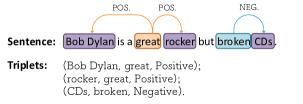
Figure 1: An example for the ASTE task illustrating Aspect terms in purple, Opinion terms with Negative sentiment in blue, and Opinion terms with Positive sentiment in orange.

In this work, we attribute the current challenges in ASTE to two main factors: 1) the longstanding overlook of the conical embedding distribution problem and 2) imprudent tagging scheme design. We critically examine the conventional 2D tagging method, commonly known as the table-filling approach, to reassess the efficacy of tagging schemes. Highlighting the critical role of tagging scheme optimization, we delve into what constitutes an ideal scheme for ASTE. We analyze the advantages of the full matrix approach over the half matrix approach and decompose the labels in the full matrix into 1) location and 2) classification. Thanks to this, we come up with a new tagging scheme with a minimum number of labels to effectively reduce the complexity of training and inference. Moreover, this tagging scheme can be well aligned with our novel contrastive learning mechanism. To the best of our knowledge, this is the first formal analysis of the tagging scheme to guide a more rational design and the first attempt to adopt token-level contrastive learning to improve the PLM representations’ distribution and facilitate the learning process.

The contributions of this work can be summarized as follows:

• We offer the first critical evaluation of the 2D tagging scheme, particularly focusing on the table-filling method. This analysis pioneers in providing a structured framework for the rational design of tagging schemes.

• We introduce a simplified tagging scheme with the least number of label categories to date, integrating a novel token-level contrastive learning approach to enhance PLM representation distribution.

• Our study addresses ASTE challenges in the context of LLMs, developing a tailored in-context learning strategy. Through evaluations on GPT 3.5-Turbo and GPT 4, we establish our method’s superior efficiency and effectiveness.

2 Related Work

2.1 ASTE

Peng et al. (2020) proposes a pipeline method to bifurcate ASTE tasks into two stages, extracting (Aspect, opinion) pairs initially and predicting sentiment polarity subsequently. However, the error propagation hampers pipeline methods, rendering them vulnerable to end-to-end counterparts. End-to-end strategies, under the sequence-labeling approach, treat ASTE as a 1D “B-I-O” tagging scheme. ET Xu et al. (2020) introduces a position-aware tagging scheme with a conditional random field (CRF) module, effectively addressing span overlapping issues unhandled by Peng et al. (2020).

Recent advances in the end-to-end paradigm delicately grasp the peculiarity of ASTE tasks and come up with a proficient 2D table-filling tagging scheme. Wu et al. (2020a) pioneer the adoption of a grid tagging scheme (GTS) for ASTE, yielding substantial performance gains. While subsequent research refines and enhances GTS, it is not devoid of drawbacks. Instances involving multi-word Aspect/Opinion constructs risk relation inconsistency and boundary insensitivity Zhang et al. (2022). To overcome these, BDTF Zhang et al. (2022) designs a boundary-driven tagging scheme, effectively reducing boundary prediction errors. Alternative research augments GTS by integrating external semantic information as structured knowledge into their models. $\mathrm{S}^{3}\mathrm{E}^{2}$ Chen et al. (2021b) retains the GTS tagging scheme while introducing novel semantic and syntactic enhancement modules between word embedding outputs and the tagging scheme. EMGCN Chen et al. (2022) offers a distinct perspective, incorporating external knowledge from four aspects, namely, Part-of-Speech Combination, Syntactic Dependency Type, Tree-based Distance, and Relative Position Distance through an exogenous hard-encoding strategy. SyMux Fei et al. (2022) contributes a unified tagging scheme capable of all ABSA subtasks synthesizing insights from incorporating GCN, syntax encoder, and representation multiplexing.

2.2 Contrastive Learning

The idea of contrastive learning can be traced back to the 1990s Le-Khac et al. (2020) and was first formally proposed by Hadsell et al. (2006). While a unified definition of contrastive learning is still absent Le-Khac et al. (2020), its essence revolves around establishing proximity among similar instances and separation between dissimilar ones within a designated metric space Jaiswal et al. (2021). The pioneer work of Wang and Isola (2020) introduced the concepts of alignment and uniformity. Alignment quantifies the closeness between akin samples’ representations, while uniformity gauges the degree that representations are distributed evenly on a unit hypersphere. Note that a representation distribution satisfying alignment and uniformity is linearly separableWu et al. (2023) and facilitates the classification. Thereby, contrastive learning boosts represent learning by improving the alignment and uniformity of the representations. However, recent investigations indicate that representation distributions in pretrained models often diverge from these expectations. Liang et al. (2021) computed similarities for randomly sampled word pairs, revealing that word embeddings in an Euclidean space cluster within a confined cone, rather than uniformly distributed.

While contrastive learning has gained popularity in diverse NLP domains Wu et al. (2020b); Giorgi et al. (2021); Gao et al. (2021); Zhang et al. (2021), its application to ASTE remains relatively unexplored. Ye et al. (2021) adopts contrastive learning into triplet extraction in a generative fashion. Wang et al. (2022) takes contrastive learning as a data augmentation approach. Yang et al. (2023) proposed an enhancement approach in pairing with two separate encoders.

3 Method

Figure 2 presents our framework. In the training phase, the process unfolds as follows: first, the input sentence is encoded by a PLM encoder, such as BERT (Devlin et al., 2018) or RoBERTa (Liu et al., 2022). Next, a single-layer classification head predicts the tagging scheme using these embeddings, and simultaneously, a contrastive loss is calculated. Then, a focal loss is computed between the predicted and ground truth tagging schemes. Finally, the focal loss and contrastive loss are weighted into the total loss. By backpropagation and convergence of the total loss, it can be expected that the predicted tagging schemes will be more and more close to their ground truth.

Algorithm 1 provides a pseudo-code description for the training process of our proposed framework.

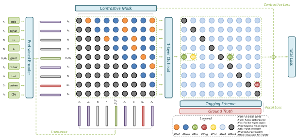
Figure 2: Schematic diagram of our proposed framework which contains: 1) a contrastive learning mechanism that aligns Aspect and Opinion; and 2) a tagging scheme encompassing 5 label classes: NULL, CTD, POS, NEU, and NEG.

3.1 Task Formulation

Given a sentence containing $|\mathcal{S}|$ tokens $\mathcal{S}_{|\mathcal{S}|}=(w_{1},w_{2},...,w_{|\mathcal{S}|})$, an ASTE algorithm should return all the triplets $\mathcal{T}_{|\mathcal{T}|}$, where $\mathcal{T}_{k}=(A_{k},O_{k},S_{k})$, $k\in\{1,2,...,|\mathcal{T}|\}$. $A_{k}$, $O_{k}$, $S_{k}$, and $|\mathcal{T}|$ denote the Aspect term, Opinion term, Sentiment polarity, and number of triplets contained in $\mathcal{S}$, respectively.

3.2 Pretrained Encoder

Given the input sentence $\mathcal{S}$ and pretrained model Encoder , it outputs the hidden word embeddings $\mathcal{H}_{|\mathcal{H}|}$:

$$\mathcal{H}_{|\mathcal{H}|}=\texttt{Encoder}(\mathcal{S}_{|\mathcal{S}|}),$$ (1)

where $\mathcal{H}_{|\mathcal{H}|}=(h_{1},h_{2},...,h_{|\mathcal{H}|})$.

3.3 Tagging Scheme

Rethinking the 2D tagging scheme:

Lemma 1. Specific to the ASTE task, when we take it as a 2D-labeling problem, we are to 1) find a set of tagging strategies to establish a 1-1 map between each triplet and its corresponding tagging matrix.

Lemma 2. In a 2D-tagging problem, there are at least three basic goals that must be met: 1) correctly identifying the (Aspect, Opinion) pairs, 2) correctly classifying the sentiment polarity of the pair based on the context, and 3) avoiding boundary errors, such as overlapping, confusion, as per Lemma 1 and conflict.

Property 1. From the above assumptions, it can be concluded that using fewer yet enough (that is, following the 1-1 map properties in Lemma 1, as well as avoiding the issues in Lemma 2) labels will make it a theoretically or heuristically better tagging scheme.

In essence, a 2D tagging scheme in ASTE serves two primary functions: locating and classifying. To develop an effective tagging scheme, three pitfalls must be avoided: overlapping, confusion, and conflict. Furthermore, building on this foundation, it is crucial to minimize the number of labels introduced to simplify the learning process.

With the above knowledge, our tagging scheme employs the full matrix so that the row-column relations can be seen as a directional graph, which naturally contains the order information. Taking advantage of this, we can see it as a coordinate system, where the row index indicates the Aspect term and the columns index indicates the Opinion. Then we can represent any triplet by a rectangular shadowed area in the matrix, which meets Lemma 3.3. Hereafter, this labeling can be taken as a “place holder”, which has supported a multi-to-one map, whilst weaker than the requirement in Lemma 3.3.

To satisfy all the conditions, we further introduce another tagging, “sentiment & beginning tag”. This tagging scheme specializes in recognizing the top-left corner of a “shadowed” area. Meanwhile, it takes a value from the sentiment polarity, i.e.Positive, Neutral, Negative. This tagging is crucial to both decide the boundary of an area and classify the sentiment polarity. It can be strictly proved that our tagging scheme perfectly meets the requirements and takes the least possible classes of labels.

Figure 3 shows a comprehensive case of our tagging scheme, in which the left matrix is an appearance of our tagging scheme, and it can be decomposed into two separate components. The middle matrix is the first component, which takes only one tag to locate the up-left beginning of an area, and the second component simply predicts a binary classification to figure out the full area.

When we add the two components together, we have the left tagging scheme, where the “Sentiment & Beginning Tag” is like a trigger (just like you click your mouse), and the “Place Holder” is like a “continued shift” (continue to hold and drag the mouse to the downright).

Note that, this design benefits the tagging scheme’s decode process. By scanning across the matrix, we only start an examination function when triggered by a beginning label like this, and then search by row and column until it meets any label except a “continued” (“CTD”).

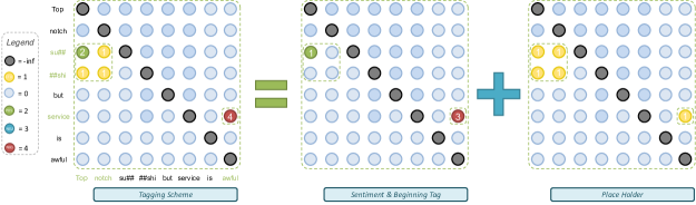
Figure 3: Decomposition of the tagging scheme into two components: 1) a beginning mark matrix with sentiment labels; and 2) a placeholder matrix denoting regions of triplets with “1”s and default regions with “0”s. Remember that each row is taken as candidates for an Aspect and each column is taken as candidates for an Opinion. Naturally, each cell in the square matrix can be seen as an ordered pair for a unique candidate of <Aspect, Opinion>.

3.4 Token-level Contrastive Learning

The motivation to adopt contrastive learning is to improve the distribution of representations output by PLMs. The core idea lies in that, after fine-tuning on a specific task, the PLM encoder should embed words with similar roles to distribute closer and drive the different ones to be farther.

Specifically in the ASTE task, for example, we take each word into either Aspect, Opinion, or None of which. So, there should be at least 3 classes for sequence tagging. Our insight is to award the model to learn a sophisticated map to embed words to cluster with those sharing the same class, given a contextual input.

Inspired by (Schroff et al., 2015), we 1) take the Euclidean distance as a negative metric on the similarity and 2) introduce a margin $\mathcal{\alpha}$ to enforce the gap between two similar hidden word representations, that is, stop pulling $\mathcal{H}_{i}$ and $\mathcal{H}_{j}$ closer when there is $\left\|\mathcal{H}_{i}-\mathcal{H}_{j}\right\|^{2}\leq\alpha$ (avoiding similar representations from squeezing too much with each other).

So, the metric of similarity is

$$\mathrm{Sim}_{i,j}=\mathbf{Sim}(\mathcal{H}_{i},\mathcal{H}_{j})=-\left\|\mathcal{H}_{i}-\mathcal{H}_{j}\right\|^{2}$$ (2)

Hence, the similarities $\mathrm{Sim}_{i,j},i,j\in\{1,2,...,|\mathcal{H}|\}$ forms a similarity matrix $\mathbf{Sim}_{|H|\times|H|}$.

To make the representations closer among tokens within the same class and farther between that of different classes, while keeping a margin of $d$, we can simply maximize $\mathrm{Sim}_{i,j}$ if $\mathcal{H}_{i}$ and $\mathcal{H}_{j}$ shares the same class and else minimize $\mathrm{Sim}_{i,j}$.

Defining a matrix $\mathbf{M_{|\mathcal{H}|\times|\mathcal{H}|}}$, it controls whether to pull (closer) or push (farther) between the hidden representation of words, that is, the “Contrastive Mask” used to calculate the contrastive loss. In Figure 2, it is the left-side strict upper-triangle matrix in blue, orange and grey.

$$\mathcal{L}_{contrastive}$$ (3)

$$= \sum_{(\mathcal{H}_{i},\mathcal{H}_{j})^{+}}\max\{\left\|\mathcal{H}_{i}-\mathcal{H}_{j}\right\|^{2},\ d\}$$

$$- \sum_{(\mathcal{H}_{i},\mathcal{H}_{j})^{-}}\min\{\left\|\mathcal{H}_{i}-\mathcal{H}_{j}\right\|^{2},\ d\}$$

$$= \sum_{i=1}^{|\mathcal{H}|}\sum_{j=i+1}^{|\mathcal{H}|}\max\{\mathbf{Sim}(\mathcal{H}_{i},\mathcal{H}_{j}),\ d\}\cdot\mathbf{M}_{i,j}.$$

$$= \sum_{i=1}^{|\mathcal{H}|}\sum_{j=1}^{|\mathcal{H}|}\big{(}\max\{\mathbf{Sim_{|\mathcal{H}|\times|\mathcal{H}|}},\ d\}\circ\mathbf{M_{|\mathcal{H}|\times|\mathcal{H}|}}\big{)}_{i,j}$$

where $\circ$ is a notation for the Hadamard product Horn (1990).

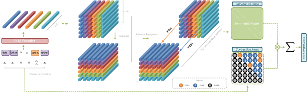
Figure 4: A more detailed illustration of our contrastive learning mechanism.

Figure 4 depicts the workflow of our contrastive learning strategy and showcases the detail of the Contrastive Mask. Note that for the purpose of contrast learning, the order of each pair of words is redundant, so using the strict upper matrix is enough and we mask the lower triangle.

Noteworthily, a PLM encoder, like BERT, encodes the same word input to different vector representations when the context is different. For example, suppose two sentences, 1) “I really just like the old school plug-in ones”, and 2) “The old school is beautiful”. Explicitly the “school” should be labelled as Aspect in the former case whilst as Opinion in the latter. For these cases, a well-learned PLM encoder will encode the unique word “school” into different representations with accordance to the context.Therefore, given that a single word can have varying meanings and associated class labels depending on its context, its representations are inherently context-specific, differing accordingly. This characteristic allows for the direct application of contrastive learning to the hidden word representations without concern for contradiction, ensuring that contextual information is preserved without loss.

3.5 classification head

We employ a streamlined single-layer linear classification head, composed sequentially of a linear classification head, dropout, layer normalization, and a GELU activation function Hendrycks and Gimpel (2016), as follows:

$$H_{1}=\texttt{LinearClsHead}(\mathcal{H}_{contrasted})$$ (4)

$$H_{3}=\texttt{LayerNorm}(H_{2})$$

$$\mathbf{Tag}_{pred}=\texttt{GELU}(H_{3})$$

3.6 Focal Loss

The tagging matrix intrinsically contains more NULL labels than valid labels (POS, NEU, NEG, and CTD). This imbalance is exacerbated by the sentiment distribution, as demonstrated in Table 5 in the Appendix. Given its naturally sparse nature, this matrix faces challenges related to both sample imbalance and hard examples. To mitigate the pronounced imbalance between positive and negative samples in the training set, we employ the Focal LossLin et al. (2017), which approach prevents an inundation of easy negatives from overwhelming the training process. Our focal loss is defined as:

$$\mathcal{L}_{focal}=\mathrm{FL}(p_{t})=-\alpha_{t}(1-p_{t})^{\gamma}\log(p_{t}),$$ (5)

where $p_{t}$ is a brief notation for

$$p_{t}=\begin{cases}p,&\textrm{if}\ y=1\\ 1-p,&\textrm{otherwise},\end{cases}$$

$\alpha_{t}$ is a factor to balance between the positive and negative samples, $y$ denotes the ground-truth class and $p\in[0,1]$ represents the estimated probability for the class. $-\big{(}1-p_{t})^{\gamma}$ modulates the canonical cross entropy (CE) loss. Notably, when $\gamma=0$ and $\alpha_{t}=0.5$, the focal loss is equivalent to a standard cross entropy loss. The final loss function is a weighted sum of the contrastive loss and the focal loss:

$$\mathcal{L}=\mathcal{L}_{focal}+\alpha\ \mathcal{L}_{contrastive},$$ (6)

where $\alpha$ is the weighting hyperparameter.

Algorithm 1 Workflow of our framework.

Modules:

Input:

Raw sentences: $\mathcal{S}_{|\mathcal{S}|}$;

Ground truth triplets: $\mathcal{T}_{|\mathcal{T}|}^{gt}$ , where

$\mathcal{T}_{k}=(A_{k},O_{k},S_{k})$, $k\in\{1,2,...,|\mathcal{T}|\}$;

classes of contrasted labels: $\mathcal{C}$.

Output:

Predicted Triplets: $\mathcal{T}_{|\mathcal{T}|}^{pred}$;

Metric: $\mathit{Precision},\mathit{Recall},\mathit{F1}$.

Algorithm:
Repeat for $N$ epochs:

1:  Hidden word representation: $\mathcal{H}_{|\mathcal{H}|}=\texttt{PLMsEncoder}(\mathcal{S}_{|\mathcal{S}|})$;

2:  Tensor Operations: $\mathcal{H}_{|\mathcal{H}|\times|\mathcal{H}|}=\texttt{expand}(\mathcal{H}_{|\mathcal{H}|})$, $\mathcal{H}_{|\mathcal{H}|\times|\mathcal{H}|}^{T}=\mathcal{H}_{|\mathcal{H}|\times|\mathcal{H}|}.\texttt{transpose}()$;

3:  Similarity matrix: $\mathbf{Sim}_{|\mathcal{H}|\times|\mathcal{H}|}=-(\mathcal{H}_{|\mathcal{H}|\times|\mathcal{H}|}-\mathcal{H}_{|\mathcal{H}|\times|\mathcal{H}|}^{T})\circ(\mathcal{H}_{|\mathcal{H}|\times|\mathcal{H}|}-\mathcal{H}_{|\mathcal{H}|\times|\mathcal{H}|}^{T})$, where   $\mathbf{Sim}_{i,j}=-\left\|\mathcal{H}_{i}-\mathcal{H}_{j}\right\|^{2}$, and $\circ$ denotes the Hadamard product;

4:  Contrastive Mask matrix: $\mathbf{M}_{|\mathcal{H}|\times|\mathcal{H}|}$, where   $\mathbf{M}_{i,j}=1$ if $\mathcal{H}_{i},mathcal{H}_{j}\in\mathcal{C}_{p},p\in{1,2,3}$ else $-1$;

5:  Contrastive loss: $\mathcal{L}_{contrastive}=\newline \sum_{i=1}^{|\mathcal{H}|}\sum_{j=1}^{|\mathcal{H}|}\big{(}\mathbf{Sim_{|\mathcal{H}|\times|\mathcal{H}|}}\circ\mathbf{M_{|\mathcal{H}|\times|\mathcal{H}|}}\big{)}_{i,j};$

6:  Predicted tagging matrix: $\mathbf{Tag}_{|\mathcal{H}|\times|\mathcal{H}|}^{pred}=\texttt{ClsHead}(\mathcal{H}_{|\mathcal{H}|\times|\mathcal{H}|},\mathcal{H}_{|\mathcal{H}|\times|\mathcal{H}|}^{T})$;

7:  Focal loss: $\mathcal{L}_{focal}=\texttt{FocalLoss}(\mathbf{Tag}_{|\mathcal{H}|\times|\mathcal{H}|}^{pred},\mathbf{Tag}_{|\mathcal{H}|\times|\mathcal{H}|}^{gt})$;

8:  Weighted Loss: $\mathcal{L}=\mathcal{L}_{focal}+\alpha\mathcal{L}_{contrastive}$.

9:  Backward propagation.

Predicted triplets:

$\mathcal{T}_{|\mathcal{T}|}^{pred}=\texttt{TaggingDecoder}(\mathbf{Tag}_{|\mathcal{H}|\times|\mathcal{H}|}^{pred})$

Metric:

$\mathit{Precision},\mathit{Recall},\mathit{F1}=\texttt{Metric}(\mathcal{T}_{|\mathcal{T}|}^{pred},\mathcal{T}_{|\mathcal{T}|}^{gt})$

4 Experiments

4.1 Implementation Details

All experiments were conducted on a single RTX 2080 Ti. The best model weight on the development set is saved and then evaluated on the test set. For the PLM encoder, the pretrained weights bert_base_uncased and roberta_base are downloaded from (Wolf et al., 2020). GPT 3.5-Turbo and GPT 4 are implemented using OpenAI API . The learning rate is $1\times 10^{-5}$ for the PLM encoder, and $1\times 10^{-3}$ for the classification head.

4.2 Datasets

We evaluate our method on two canonical ASTE datasets derived from the SemEval Challenges Pontiki et al. (2014, 2015, 2016). These datasets serve as benchmarks in the majority of Aspect-based Sentiment Analysis (ABSA) research. The first dataset, denoted as $\mathcal{D}_{1}$, is the Aspect-oriented Fine-grained Opinion Extraction (AFOE) dataset introduced by Wu et al. (2020a). The second dataset, denoted as $\mathcal{D}_{2}$, is a refined version by Xu et al. (2020), building upon the work of Peng et al. (2020). Further details are provided in Table 5.

4.3 Baselines

We evaluate our method against various techniques including pipeline, sequence-labeling, MRC-based, table-filling and LLM-based approaches. Detailed descriptions of each method can be found in the Appendix Table 8.

Methods	14Res				14Lap				15Res				16Res
	P	R	F1		P	R	F1		P	R	F1		P	R	F1
Pipeline
$\textrm{Two-stage}^{\natural}$ Peng et al. (2020)	43.24	63.66	51.46		37.38	50.38	42.87		48.07	57.51	52.32		46.96	64.24	54.21
$\textrm{Li-unified-R+PD}^{\sharp}$ Peng et al. (2020)	40.56	44.28	42.34		41.04	67.35	51.00		44.72	51.39	47.82		37.33	54.51	44.31
Sequence-tagging
Span-BART Yan et al. (2021)	65.52	64.99	65.25		61.41	56.19	58.69		59.14	59.38	59.26		66.60	68.68	67.62
JET Xu et al. (2020)	70.56	55.94	62.40		55.39	47.33	51.04		64.45	51.96	57.53		70.42	58.37	63.83
MRC-based
Dual-MRC Mao et al. (2021)	71.55	69.14	70.32		57.39	53.88	55.58		63.78	51.87	57.21		68.60	66.24	67.40
$\textrm{BMRC}^{\dagger}$ Chen et al. (2021a)	72.17	65.43	68.64		65.91	52.15	58.18		62.48	55.55	58.79		69.87	65.68	67.35
COM-MRC Zhai et al. (2022)	75.46	68.91	72.01		62.35	58.16	60.17		68.35	61.24	64.53		71.55	71.59	71.57
Triple-MRC Zou et al. (2024)	-	-	72.45		-	-	60.72		-	-	62.86		-	-	68.65
Table-filling
GTS Wu et al. (2020a)	67.76	67.29	67.50		57.82	51.32	54.36		62.59	57.94	60.15		66.08	66.91	67.93
Double-encoder Jing et al. (2021)	67.95	71.23	69.55		62.12	56.38	59.11		58.55	60.00	59.27		70.65	70.23	70.44
EMC-GCN Chen et al. (2022)	71.21	72.39	71.78		61.70	56.26	58.81		61.54	62.47	61.93		65.62	71.30	68.33
BDTF Zhang et al. (2022)	75.53	73.24	74.35		68.94	55.97	61.74		68.76	63.71	66.12		71.44	73.13	72.27
STAGE-1D Liang et al. (2023)	79.54	68.47	73.58		71.48	53.97	61.49		72.05	58.23	64.37		78.38	69.10	73.45
STAGE-2D Liang et al. (2023)	78.51	69.3	73.61		70.56	55.16	61.88		72.33	58.93	64.94		77.67	68.44	72.75
STAGE-3D Liang et al. (2023)	78.58	69.58	73.76		71.98	53.86	61.58		73.63	57.9	64.79		76.67	70.12	73.24
DGCNAP Li et al. (2023)	72.90	68.69	70.72		62.02	53.79	57.57		62.23	60.21	61.19		69.75	69.44	69.58
LLM-based
GPT 3.5 zero-shot	44.88	55.13	49.48		30.04	41.04	34.69		36.02	53.40	43.02		39.92	57.78	47.22
GPT 3.5 few-shots	52.36	54.63	53.47		29.91	36.04	32.69		45.48	61.44	52.01		49.50	67.12	56.98
GPT 4 zero-shot	32.99	38.13	35.37		17.81	22.55	19.90		27.85	37.73	32.05		32.17	43.00	36.80
GPT 4 few-shots	47.25	49.20	48.20		26.04	33.64	29.35		39.94	51.13	44.85		43.72	54.86	48.66
Ours
ContrASTE	76.1	75.08	75.59		66.82	60.68	63.61		66.50	63.86	65.15		75.52	74.14	74.83

Table 1: Experimental results on $\mathcal{D}_{2}$ Xu et al. (2020). The best results are highlighted in bold, while the second best results are underlined.

4.4 Performance on ASTE Tasks

We evaluate ASTE performance using the widely accepted (Precision, Recall, F1) metrics. The result on dataset $\mathcal{D}_{2}$ can be found in Table 1 and on $\mathcal{D}_{1}$ is presented in Appendix Table 7. The best results are indicated in bold, while the second best results are underlined. Our proposed method consistently achieves state-of-the-art performance or ranks second across all evaluated cases.

Significantly, on dataset $\mathcal{D}_{1}$, proposed method achieves a substantial improvement of 3.08 percentage points in F1 score on the 14Lap subset. This improvement is particularly noteworthy considering that the best score on this dataset is the lowest among all the datasets, showcasing our ability to effectively handle challenging instances. Moreover, on the 14Res subset, our F1 score surpasses 76.00+, which, to the best of our knowledge, is the highest reported performance.

Turning to dataset $\mathcal{D}_{2}$, our method outperforms all state-of-the-art approaches by more than 1 percentage point on the 14Res, 14Lap, and 16Res subsets. Only on the 16Res subset, the BDTF method (Zhang et al., 2022) achieves a slightly better performance.

It is worth highlighting that, compared to previous methods, our approach achieves significantly higher recall in the majority of cases in both $\mathcal{D}_{1}$ and $\mathcal{D}_{2}$, without significantly compromising precision. This observation underscores the robustness of our method in minimizing the omission of true triplets. This behavior can be attributed to our contrastive learning process, where the learned representations contribute to accurate predictions, thereby enhancing the effectiveness of triplet identification.

4.5 Performance on Other ABSA Tasks

Our method can also effectively handle other ABSA subtasks, including Aspect Extraction (AE), Opinion Extraction (OE), and Aspect Opinion Pair Extraction (AOPE). AE aims to extract all the (Aspect) terms, OE aims to extract all the Opinion terms, and AOPE aims to extract all the (Aspect, Opinion) pairs from raw text. The results for these tasks are presented in Table 6 in the Appendix, where our method consistently achieves best F1-scores across nearly all tasks.

Models	$\mathcal{D}_{1}$					$\mathcal{D}_{2}$
	14Res	14Lap	15Res	16Res		14Res	14Lap	15Res	16Res
ContrASTE	76.00	64.07	65.43	71.80		75.59	63.61	65.15	74.83
w/o. RoBERTa	74.12	63.18	62.95	69.41		72.66	62.15	63.25	70.71
$\Delta$F_1	-1.88	-0.89	-2.48	-2.39		-2.93	-1.46	-1.90	-4.12
w/o. contr	72.61	61.94	58.14	68.16		71.72	61.49	58.11	68.03
$\Delta$F_1	-3.39	-2.13	-7.29	-3.64		-3.87	-2.12	-7.04	-6.80
w/o. tag	67.78	54.98	60.75	62.62		65.83	54.98	58.73	67.63
$\Delta$F_1	-8.22	-9.09	-4.68	-9.18		-9.76	-8.63	-6.42	-7.20

Table 2: Ablation study on F1, where “w/o. RoBERTa” denotes “Replace RoBERTa with bert-base-uncased”, “w/o. contr” denotes without the contrastive learning mechanism, and “w/o. tag” denotes “replace our tagging scheme with a baseline”.

5 Analysis

5.1 Ablation Study

Encoder. In the ablation experiment part, by replacing RoBERTa by BERT, The results obtained declined slightly while still yield most other methods.

Contrastive Learning. First, we deactivating the contrastive mechanism in our method (denoting “w/o. contr”) by setting the coefficient of the contrastive loss to 0. The results in Table 2 illustrate a significant F1-score decrease of $0.22\sim 2.93$ percentage points.

Tagging Scheme. Third, we substitute our proposed scheme with the conventional GTS tagging scheme Wu et al. (2020a), which results in a significant performance decline (Table 2) by $1.46\sim 6.14$ percentage points. This indicates that the contrastive learning methods, within our framework, is of strong reliance on an appropriate tagging scheme. This reinforces the effectiveness of our straightforward yet impactful tagging scheme.

5.2 Effect of Contrastive Learning

In Appendix Figure 5 an example is shown of how contrastive learning has improved the representation, where the left subplot is the tokens output by RoBERTa without contrastive learning, and the right one is with contrastive learning. Note that the Principal Component Analysis (PCA) (Maćkiewicz and Ratajczak, 1993) is adopted to reduce the dimensions of the vectors to 2.

5.3 Efficiency Analysis

Table 3: Efficiency Analysis

Model	Memory	Num Params	Epoch Time	Inf Time	F1(%)	Device
Span-ASTE	3.173GB	-	108s	-	71.62	Tesla v100
BDTF	8.103GB	-	135s	-	74.73	Tesla v100
GPT 3.5-Turbo	$>80GB$	175B	-	0.83s	49.48	OpenAI API
GPT 4	$>80GB$	1760B	-	1.56s	35.37	OpenAI API
Ours	7.11GB	0.12B	10s	0.01s	76.00	2080 Ti

Table 4: Tagging Scheme Comparisons

Method	Num Tags	Linguistic Features	Half/Full Matrix
GTS	6	None	Half
Double-encoder	9	None	Half
EMC-GCN	10	4 Groups	Full
BDTF	$2\times 2\times 3$	None	Half
STAGE	$2\times 2\times 4$	None	Half
DGCNAP	6	POS-tagging	Half
Ours	$5$	None	Full

Table 3 shows an efficiency analysis, where our method is in significantly higher efficiency. While our approach demonstrates efficient management of memory and parameter utilization, surpassing other methods in terms of runtime performance, it is crucial to note the unsatisfactory performance of LLM-based methods, as demonstrated by Table 7, Table 1 and Table 9. This observation highlights that employing a general LLM with a large number of parameters does not yield desirable results in specific tasks like ASTE, even with the assistance of few-shot memorizing processes. Moreover, the incorporation of LLM introduces a significant computational resource overhead in general application scenarios. Although fine-tuning the parameters of LLM itself may offer some improvement, there exists a risk of collapsive forgetting. Furthermore, Table 4 provides a comparative analysis of tagging schemes. Our method achieves its objective without the need for additional linguistic information and utilizes fewer taggings.

6 Conclusion

In this work, we have introduced an elegant and efficient framework for ASTE, achieving SOTA performance. Our approach is built upon two effective components: a new tagging scheme and a novel token-level contrastive learning implementation. The ablation study demonstrates the synergy between these components, reducing the need for complex model designs and external information enhancements. The limitation of this work lies in that there lefts potential to further optimize the framework by investigating various classification head strategies.

Appendix A Appendix

Datasets			#S	#A	#O	#S1	#S2	#S3	#T
14Res	$\mathcal{D}_{1}$	Train	1259	1008	849	1456	164	446	2066
		Dev	315	358	321	352	44	93	489
		Test	493	591	433	651	59	141	851
	$\mathcal{D}_{2}$	Train	1266	986	844	1692	166	480	2338
		Dev	310	396	307	404	54	119	577
		Test	492	579	437	773	66	155	994
14Lap	$\mathcal{D}_{1}$	Train	899	731	693	691	107	466	1264
		Dev	225	303	237	173	42	118	333
		Test	332	411	330	305	62	101	468
	$\mathcal{D}_{2}$	Train	906	733	695	817	126	517	1460
		Dev	219	268	237	169	36	141	346
		Test	328	400	329	364	63	116	543
15Res	$\mathcal{D}_{1}$	Train	603	585	485	668	24	179	871
		Dev	151	182	161	156	8	41	205
		Test	325	353	307	293	19	124	436
	$\mathcal{D}_{2}$	Train	605	582	462	783	25	205	1013
		Dev	148	191	183	185	11	53	249
		Test	322	347	310	317	25	143	485
16Res	$\mathcal{D}_{1}$	Train	863	775	602	890	43	280	1213
		Dev	216	270	237	224	8	66	298
		Test	328	342	282	360	25	72	457
	$\mathcal{D}_{2}$	Train	857	759	623	1015	50	329	1394
		Dev	210	251	221	252	11	76	339
		Test	326	338	282	407	29	78	514

Table 5: Statistic information of our two experiment datasets: “#S”, “#T”, “#A”, and “#O” denote the numbers of “Sentences”, “Triplets”, “Aspects”, and “Opinions”; “#S1”, “#S2”, #S3” denote the numbers of sentiments “Positive”, “Neutral” and “Negative”, respectively.

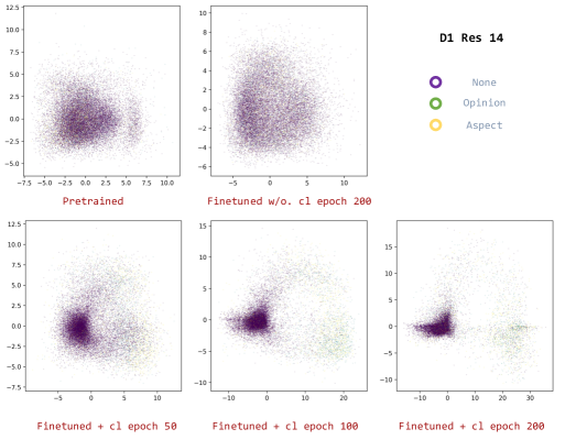
Figure 5: A plot of the hidden word representation, where the dimension is reduced to 2 for convenience of display. “Pretrained” means the model with official released version of weights. “Finetuned” means the model is a finetuned version on ASTE task for certain epochs. “w/o. cl” means the model is trained without contrastive learning loss. “+ cl” means the model is trained with contrastive learning. All the plotted results are from experiment carried on $\mathcal{D}_{1}$ 14Res.

Methods	14Res				14Lap				15Res				16Res
	AE	OE	AOPE		AE	OE	AOPE		AE	OE	AOPE		AE	OE	AOPE
CMLA	81.22	83.07	48.95		78.68	77.95	44.10		76.03	74.67	44.60		74.20	72.20	50.00
RINANTE	81.34	83.33	46.29		77.13	75.34	29.70		73.38	75.40	35.40		72.82	70.45	30.70
Li-unified	81.62	85.26	55.34		78.54	77.55	52.56		74.65	74.25	56.85		73.36	73.87	53.75
GTS	83.82	85.04	75.53		79.52	78.61	65.67		78.22	79.31	67.53		75.80	76.38	74.62
Dual-MRC	86.60	86.22	77.68		80.44	79.90	63.37		75.08	77.52	64.97		76.87	77.90	75.71
ContrASTE (Ours)	86.55	87.04	79.60		82.62	83.41	73.23		86.53	83.05	73.87		85.48	87.06	76.29
$\Delta$F1	-0.05	0.82	1.92		2.18	3.51	7.56		8.31	3.74	6.34		8.61	9.16	0.58

Table 6: F1-score performance on other ABSA tasks: AE, OE, and AOPE. The test is implemented on $\mathcal{D}_{1}$. Results of other models are retrieved from Fei et al. (2022).

Methods	14Res				14Lap				15Res				16Res
	P	R	F1		P	R	F1		P	R	F1		P	R	F1
Pipeline
OTE-MTL Zhang et al. (2020)	-	-	45.05		-	-	59.67		-	-	48.97		-	-	55.83
$\textrm{Li-unified-R+PD}^{\sharp}$ Peng et al. (2020)	41.44	68.79	51.68		42.25	42.78	42.47		43.34	50.73	46.69		38.19	53.47	44.51
RI-NANTE+ Dai and Song (2019)	31.42	39.38	34.95		21.71	18.66	20.07		29.88	30.06	29.97		25.68	22.30	23.87
$\textrm{CMLA+C-GCN}^{\flat}$ Wang et al. (2017)	72.22	56.35	63.17		60.69	47.25	53.03		64.31	49.41	55.76		66.61	59.23	62.70
Two-satge♮ Peng et al. (2020)	58.89	60.41	59.64		48.62	45.52	47.02		51.7	46.04	48.71		59.25	58.09	59.67
Sequence-tagging
Span-BART Yan et al. (2021)	-	-	72.46		-	-	57.59		-	-	60.10		-	-	69.98
JET Xu et al. (2020)	67.97	60.32	63.92		58.47	43.67	50.00		58.35	51.43	54.67		64.77	61.29	62.98
MRC based
BMRC† Chen et al. (2021a)	71.32	70.09	70.69		65.12	54.41	59.27		63.71	58.63	61.05		67.74	68.56	68.13
COM-MRC Zhai et al. (2022)	76.45	69.67	72.89		64.73	56.09	60.09		68.50	59.74	63.65		72.80	70.85	71.79
Table-filling
$\mathrm{S}^{3}\mathrm{E}^{2}$ Chen et al. (2021b)	69.08	64.55	66.74		59.43	46.23	52.01		61.06	56.44	58.66		71.08	63.13	66.87
GTS Wu et al. (2020a)	70.92	69.49	70.20		57.52	51.92	54.58		59.29	58.07	58.67		68.58	66.60	67.58
EMC-GCN Chen et al. (2022)	71.85	72.12	71.78		61.46	55.56	58.32		59.89	61.05	60.38		65.08	71.66	68.18
BDTF Zhang et al. (2022)	76.71	74.01	75.33		68.30	55.10	60.99		66.95	65.05	65.97		73.43	73.64	73.51
DGCNAP Li et al. (2023)	71.83	68.77	70.26		66.46	54.34	58.74		62.03	57.18	59.49		69.39	72.20	70.77
LLM-based
GPT 3.5 zero-shot	39.21	56.17	46.18		26.21	40.69	31.88		31.21	52.75	39.21		35.28	59.64	44.34
GPT 3.5 few-shots	44.73	58.87	50.84		29.63	37.69	33.18		37.27	56.42	44.89		43.15	60.75	50.46
GPT 4 zero-shot	27.34	37.13	31.49		16.50	24.41	19.69		25.60	39.22	30.98		28.39	43.64	35.79
GPT 4 few-shots	41.48	52.06	46.17		28.79	39.83	33.42		38.04	58.02	45.96		40.89	62.50	49.44
Ours
ContrASTE	75.87	76.12	76.00		67.45	61.01	64.07		66.84	64.08	65.43		69.38	74.40	71.80

Table 7: Experimental results on $\mathcal{D}_{1}$ Wu et al. (2020a). The best results are highlighted in bold, while the second best results are underlined.

Methods	Brief Introduction
Pipeline
OTE-MTL Zhang et al. (2020)	It proposes a multi-task learning framework including two parts: aspect and opinion tagging, along with word-level sentiment dependency parsing. This approach simultaneously extracts aspect and opinion terms while parsing sentiment dependencies using a biaffine scorer. Additionally, it employs triplet decoding based on the aforementioned outputs during inference to facilitate triplet extraction.
Li-unified-R+PD Peng et al. (2020)	It proposes an unified tagging scheme, Li-unified-R, to assist target boundary detection. Two stacked LSTMs are employed to complete aspect-based sentiment prediction and the sequence labeling.
CMLA+C-GCN Wang et al. (2017)	It facilitates triplet extraction by modelling the interaction between the aspects and opinions.
Two-satge Peng et al. (2020)	It decomposes triplet extraction to two stages: 1) predicting unified aspect-sentiment and opinion tags; and 2) pairing the two results from stage one.
RI-NANTE+ Dai and Song (2019)	It adopts the same sentiment triplets extracting method as that of CMLA+, but it incorporates a novel LSTM-CRF mechanism and fusion rules to capture word dependencies within sentences.
Sequence-tagging
Span-BART Yan et al. (2021)	It redefines triplet extraction within an end-to-end framework by utilizing a sequence composed of pointer and sentiment class indexes. This is achieved by leveraging the pretrained sequence-to-sequence model BART to address ASTE.
JET Xu et al. (2020)	It extracts triplets jointly by designing a position-aware sequence-tagging scheme to extract the triplets and capturing the rich interactions among the elements.
MRC-based
Dual-MRC Mao et al. (2021)	It proposes a MRC-based solution for ASTE by jointly training two BERT-MRC models with parameters sharing.
BMRC Chen et al. (2021a)	It introduces a bidirectional MRC (BMRC) framework for ASTE, employing three query types: non-restrictive extraction queries, restrictive extraction queries, and sentiment classification queries. The framework synergistically leverages two directions, one for sequential recognition of aspect-opinion-sentiment and the other for sequential recognition of opinion-aspects-sentiment expressions.
Table-filling
GTS Wu et al. (2020a)	It proposes a novel 2D tagging scheme to address ASTE in an end-to-end fashion only with one unified grid tagging task. It also devises an effective inference strategy on GTS that utilizes mutual indication between different opinion factors to achieve more accurate extraction.
Double-encoder Jing et al. (2021)	It proposes a dual-encoder model that capitalizes on encoder sharing while emphasizing differences to enhance effectiveness. One of the encoders, referred to as the pair encoder, specifically concentrates on candidate aspect-opinion pair classification, while the original encoder retains its focus on sequence labeling.
$\mathrm{S}^{3}\mathrm{E}^{2}$ Chen et al. (2021b)	It represents the semantic and syntactic relationships between word pairs, employs GNNs for encoding, and applies a more efficient inference strategy.
EMC-GCN Chen et al. (2022)	It employs a biaffine attention module to embed ten types of relations within sentences, transforming the sentence into a multi-channel graph while incorporating various linguistic features to enhance performance. Additionally, the method introduces an effective strategy for refining word-pair representations, aiding in the determination of whether word pairs are a match or not.
LLM-based
zero-shot	Performing aspect-based sentiment analysis using an LLM. The specific method involves inputting a prompted sentence and directly outputting the corresponding [A, O, S] triplets. An example of the text given to the LLM, with the prompt added, is as follows: "Perform aspect-based sentiment analysis on the provided text and return triplets as [Aspect, Opinion, Sentiment]. You only need to provide the triplets, no additional explanations are required. The provided text: {sentence}"
few-shots	Building upon the zero-shot method, a small number of examples from the training set are added to the prompted sentence: "Perform aspect-based sentiment analysis on the provided text and return triplets as [Aspect, Opinion, Sentiment]. For example: input: {train sentence} output: {train triplets}, … (some other examples). You only need to provide the triplets, no additional explanations are required. The provided text: {sentence}"

Table 8: Baselines methods with brief introduction.

Sentence	Ground Truth	Predictions
		GPT-3.5 zero-shot	GPT-3.5 few-shots	GPT-4 zero-shot	GPT-4 few-shots
It is a cozy place to go with a couple of friends.	[place, cozy, positive]	[place, cozy, positive], [friends, couple of, positive]	[place, cozy, positive]	[place, cozy, positive] [going with friends, a couple of, positive]	[place, cozy, positive]
This place has the best sushi in the city.	[sushi, best, positive]	[sushi, best, positive], [place, best, positive], [city, best, positive]	[sushi, best, positive]	[sushi, the best, positive], [place, This, neutral], [city, in the, neutral]	[sushi, best, positive]
Disappointingly, their wonderful Saketini has been taken off the bar menu.	[Saketini, wonderful, positive], [bar menu, Disappointingly, negative]	[Saketini, wonderful, positive], [bar menu, taken off, negative]	[Saketini, taken off, negative]	[Saketini, has been taken off the bar menu, negative], [bar menu, wonderful, positive]	[Saketini, wonderful, positive], [bar menu, taken off, negative]
I went in one day asking for a table for a group and was greeted by a very rude hostess.	[hostess, rude, negative]	[hostess, rude, negative]	[hostess, rude, negative]	[table for a group, asking, neutral], [hostess, very rude, negative]	[table for a group, asking, neutral], [hostess, very rude, negative]
But make sure you have enough room on your credit card as the bill will leave a big dent in your wallet.	[bill, big, negative]	[credit card, enough room, positive], [bill, big dent, negative], [wallet, big dent, negative]	[credit card, enough room, negative], [bill, big dent, negative], [wallet, big dent, negative]	[room on your credit card, enough, positive], [bill, will leave a big dent in your wallet, negative]	[bill, big dent, negative]

Table 9: In summary, there are several challenges observed in the performance of GPT models concerning triplets. Firstly, there is a prominent issue of "hard" matching, where GPT models tend to introduce additional modifiers or adverbs in the opinion component, leading to a lack of exact correspondence. Secondly, during zero-shot inference, GPT models tend to generate multiple predicted triplets, resulting in decreased precision. This behavior particularly hampers the precision of the model’s predictions. Thirdly, inconsistencies arise in handling triplets involving structures such as [A, O1 and O2, S] and [A, O1, S], [A, O2, S]. This inconsistency is challenging to mitigate due to its dependence on annotation practices and conventions. Upon closer examination, the issues observed do not appear to be as pronounced as indicated by the evaluation metrics. Rather, they often manifest as cases where the general idea is correctly captured, but the precise format or phrasing does not align perfectly. Notably, the performance of GPT-4 deteriorates due to its occasional tendency to not merely "extract" fragments from sentences but to generate its own summarizations. Consequently, evaluating against triplets that originate solely from annotated sentences poses a challenge in achieving alignment. Furthermore, GPT-4 exhibits a proclivity for extracting longer sequences of words as aspects or opinions, while GPT-3.5 tends to produce shorter sequences that better conform to typical annotation scenarios.

References

- Chen et al. (2022) Hao Chen, Zepeng Zhai, Fangxiang Feng, Ruifan Li, and Xiaojie Wang. 2022. Enhanced multi-channel graph convolutional network for aspect sentiment triplet extraction. In Proceedings of the 60th Annual Meeting of the Association for Computational Linguistics (Volume 1: Long Papers), pages 2974–2985.
- Chen et al. (2021a) Shaowei Chen, Yu Wang, Jie Liu, and Yuelin Wang. 2021a. Bidirectional machine reading comprehension for aspect sentiment triplet extraction. In Proceedings of the AAAI conference on artificial intelligence, volume 35, pages 12666–12674.
- Chen et al. (2021b) Zhexue Chen, Hong Huang, Bang Liu, Xuanhua Shi, and Hai Jin. 2021b. Semantic and syntactic enhanced aspect sentiment triplet extraction. arXiv preprint arXiv:2106.03315.
- Dai and Song (2019) Hongliang Dai and Yangqiu Song. 2019. Neural aspect and opinion term extraction with mined rules as weak supervision. In Proceedings of the 57th Annual Meeting of the Association for Computational Linguistics, pages 5268–5277.
- Devlin et al. (2018) Jacob Devlin, Ming-Wei Chang, Kenton Lee, and Kristina Toutanova. 2018. Bert: Pre-training of deep bidirectional transformers for language understanding. arXiv preprint arXiv:1810.04805.
- Fei et al. (2022) Hao Fei, Fei Li, Chenliang Li, Shengqiong Wu, Jingye Li, and Donghong Ji. 2022. Inheriting the wisdom of predecessors: A multiplex cascade framework for unified aspect-based sentiment analysis. In Proceedings of the Thirty-First International Joint Conference on Artificial Intelligence, IJCAI, pages 4096–4103.
- Gao et al. (2021) Tianyu Gao, Xingcheng Yao, and Danqi Chen. 2021. Simcse: Simple contrastive learning of sentence embeddings. In 2021 Conference on Empirical Methods in Natural Language Processing, EMNLP 2021, pages 6894–6910. Association for Computational Linguistics (ACL).
- Giorgi et al. (2021) John Giorgi, Osvald Nitski, Bo Wang, and Gary Bader. 2021. Declutr: Deep contrastive learning for unsupervised textual representations. In Proceedings of the 59th Annual Meeting of the Association for Computational Linguistics and the 11th International Joint Conference on Natural Language Processing (Volume 1: Long Papers), pages 879–895.
- Hadsell et al. (2006) Raia Hadsell, Sumit Chopra, and Yann LeCun. 2006. Dimensionality reduction by learning an invariant mapping. In 2006 IEEE computer society conference on computer vision and pattern recognition (CVPR’06), volume 2, pages 1735–1742. IEEE.
- Hendrycks and Gimpel (2016) Dan Hendrycks and Kevin Gimpel. 2016. Gaussian error linear units (gelus). arXiv preprint arXiv:1606.08415.
- Horn (1990) Roger A Horn. 1990. The hadamard product. In Proc. Symp. Appl. Math, volume 40, pages 87–169.
- Jaiswal et al. (2021) Ashish Jaiswal, Ashwin Ramesh Babu, Mohammad Zaki Zadeh, Debapriya Banerjee, and Fillia Makedon. 2021. A survey on contrastive self-supervised learning. Technologies, 9(1).
- Jing et al. (2021) Hongjiang Jing, Zuchao Li, Hai Zhao, and Shu Jiang. 2021. Seeking common but distinguishing difference, a joint aspect-based sentiment analysis model. In Proceedings of the 2021 Conference on Empirical Methods in Natural Language Processing, pages 3910–3922.
- Le-Khac et al. (2020) Phuc H Le-Khac, Graham Healy, and Alan F Smeaton. 2020. Contrastive representation learning: A framework and review. Ieee Access, 8:193907–193934.
- Li et al. (2023) Yanbo Li, Qing He, and Damin Zhang. 2023. Dual graph convolutional networks integrating affective knowledge and position information for aspect sentiment triplet extraction. Frontiers in Neurorobotics, 17.
- Liang et al. (2023) Shuo Liang, Wei Wei, Xian-Ling Mao, Yuanyuan Fu, Rui Fang, and Dangyang Chen. 2023. Stage: span tagging and greedy inference scheme for aspect sentiment triplet extraction. In Proceedings of the AAAI Conference on Artificial Intelligence, volume 37, pages 13174–13182.
- Liang et al. (2021) Yuxin Liang, Rui Cao, Jie Zheng, Jie Ren, and Ling Gao. 2021. Learning to remove: Towards isotropic pre-trained bert embedding. In Artificial Neural Networks and Machine Learning–ICANN 2021: 30th International Conference on Artificial Neural Networks, Bratislava, Slovakia, September 14–17, 2021, Proceedings, Part V 30, pages 448–459. Springer.
- Lin et al. (2017) Tsung-Yi Lin, Priya Goyal, Ross Girshick, Kaiming He, and Piotr Dollár. 2017. Focal loss for dense object detection. In Proceedings of the IEEE international conference on computer vision, pages 2980–2988.
- Liu et al. (2022) Shu Liu, Kaiwen Li, and Zuhe Li. 2022. A robustly optimized bmrc for aspect sentiment triplet extraction. In Proceedings of the 2022 Conference of the North American Chapter of the Association for Computational Linguistics: Human Language Technologies, pages 272–278.
- Maćkiewicz and Ratajczak (1993) Andrzej Maćkiewicz and Waldemar Ratajczak. 1993. Principal components analysis (pca). Computers & Geosciences, 19(3):303–342.
- Mao et al. (2021) Yue Mao, Yi Shen, Chao Yu, and Longjun Cai. 2021. A joint training dual-mrc framework for aspect based sentiment analysis. In Proceedings of the AAAI conference on artificial intelligence, volume 35, pages 13543–13551.
- Peng et al. (2020) Haiyun Peng, Lu Xu, Lidong Bing, Fei Huang, Wei Lu, and Luo Si. 2020. Knowing what, how and why: A near complete solution for aspect-based sentiment analysis. In Proceedings of the AAAI conference on artificial intelligence, volume 34, pages 8600–8607.
- Pontiki et al. (2014) Eleni Pontiki, Dimitra Hadjipavlou-Litina, Konstantinos Litinas, and George Geromichalos. 2014. Novel cinnamic acid derivatives as antioxidant and anticancer agents: Design, synthesis and modeling studies. Molecules, 19(7):9655–9674.
- Pontiki et al. (2015) Maria Pontiki, Dimitrios Galanis, Harris Papageorgiou, Suresh Manandhar, and Ion Androutsopoulos. 2015. Semeval-2015 task 12: Aspect based sentiment analysis. In Proceedings of the 9th international workshop on semantic evaluation (SemEval 2015), pages 486–495.
- Pontiki et al. (2016) Maria Pontiki, Dimitris Galanis, Haris Papageorgiou, Ion Androutsopoulos, Suresh Manandhar, Mohammed AL-Smadi, Mahmoud Al-Ayyoub, Yanyan Zhao, Bing Qin, Orphée De Clercq, et al. 2016. Semeval-2016 task 5: Aspect based sentiment analysis. In ProWorkshop on Semantic Evaluation (SemEval-2016), pages 19–30. Association for Computational Linguistics.
- Schroff et al. (2015) Florian Schroff, Dmitry Kalenichenko, and James Philbin. 2015. Facenet: A unified embedding for face recognition and clustering. In Proceedings of the IEEE conference on computer vision and pattern recognition, pages 815–823.
- Wang et al. (2022) Bing Wang, Liang Ding, Qihuang Zhong, Ximing Li, and Dacheng Tao. 2022. A contrastive cross-channel data augmentation framework for aspect-based sentiment analysis. In Proceedings of the 29th International Conference on Computational Linguistics, pages 6691–6704.
- Wang and Isola (2020) Tongzhou Wang and Phillip Isola. 2020. Understanding contrastive representation learning through alignment and uniformity on the hypersphere. In International Conference on Machine Learning, pages 9929–9939. PMLR.
- Wang et al. (2017) Wenya Wang, Sinno Jialin Pan, Daniel Dahlmeier, and Xiaokui Xiao. 2017. Coupled multi-layer attentions for co-extraction of aspect and opinion terms. In Proceedings of the Thirty-First AAAI Conference on Artificial Intelligence, pages 3316–3322.
- Wolf et al. (2020) Thomas Wolf, Lysandre Debut, Victor Sanh, Julien Chaumond, Clement Delangue, Anthony Moi, Pierric Cistac, Tim Rault, Rémi Louf, Morgan Funtowicz, et al. 2020. Transformers: State-of-the-art natural language processing. In Proceedings of the 2020 conference on empirical methods in natural language processing: system demonstrations, pages 38–45.
- Wu et al. (2023) Jing Wu, Jennifer Hobbs, and Naira Hovakimyan. 2023. Hallucination improves the performance of unsupervised visual representation learning. In Proceedings of the IEEE/CVF International Conference on Computer Vision, pages 16132–16143.
- Wu et al. (2020a) Zhen Wu, Chengcan Ying, Fei Zhao, Zhifang Fan, Xinyu Dai, and Rui Xia. 2020a. Grid tagging scheme for aspect-oriented fine-grained opinion extraction. In Findings of the Association for Computational Linguistics: EMNLP 2020, pages 2576–2585.
- Wu et al. (2020b) Zhuofeng Wu, Sinong Wang, Jiatao Gu, Madian Khabsa, Fei Sun, and Hao Ma. 2020b. Clear: Contrastive learning for sentence representation. arXiv preprint arXiv:2012.15466.
- Xu et al. (2020) Lu Xu, Hao Li, Wei Lu, and Lidong Bing. 2020. Position-aware tagging for aspect sentiment triplet extraction. In Proceedings of the 2020 Conference on Empirical Methods in Natural Language Processing (EMNLP), pages 2339–2349.
- Yan et al. (2021) Hang Yan, Junqi Dai, Tuo Ji, Xipeng Qiu, and Zheng Zhang. 2021. A unified generative framework for aspect-based sentiment analysis. In Proceedings of the 59th Annual Meeting of the Association for Computational Linguistics and the 11th International Joint Conference on Natural Language Processing (Volume 1: Long Papers), pages 2416–2429.
- Yang et al. (2023) Fan Yang, Mian Zhang, Gongzhen Hu, and Xiabing Zhou. 2023. A pairing enhancement approach for aspect sentiment triplet extraction. arXiv preprint arXiv:2306.10042.
- Ye et al. (2021) Hongbin Ye, Ningyu Zhang, Shumin Deng, Mosha Chen, Chuanqi Tan, Fei Huang, and Huajun Chen. 2021. Contrastive triple extraction with generative transformer. In Proceedings of the AAAI conference on artificial intelligence, volume 35, pages 14257–14265.
- Zhai et al. (2022) Zepeng Zhai, Hao Chen, Fangxiang Feng, Ruifan Li, and Xiaojie Wang. 2022. Com-mrc: A context-masked machine reading comprehension framework for aspect sentiment triplet extraction. In Proceedings of the 2022 Conference on Empirical Methods in Natural Language Processing, pages 3230–3241.
- Zhang et al. (2020) Chen Zhang, Qiuchi Li, Dawei Song, and Benyou Wang. 2020. A multi-task learning framework for opinion triplet extraction. In Findings of the Association for Computational Linguistics: EMNLP 2020, pages 819–828.
- Zhang et al. (2021) Dejiao Zhang, Feng Nan, Xiaokai Wei, Shang-Wen Li, Henghui Zhu, Kathleen Mckeown, Ramesh Nallapati, Andrew O Arnold, and Bing Xiang. 2021. Supporting clustering with contrastive learning. In Proceedings of the 2021 Conference of the North American Chapter of the Association for Computational Linguistics: Human Language Technologies, pages 5419–5430.
- Zhang et al. (2022) Yice Zhang, Yifan Yang, Yihui Li, Bin Liang, Shiwei Chen, Yixue Dang, Min Yang, and Ruifeng Xu. 2022. Boundary-driven table-filling for aspect sentiment triplet extraction. In Proceedings of the 2022 Conference on Empirical Methods in Natural Language Processing, pages 6485–6498.
- Zou et al. (2024) Wang Zou, Wubo Zhang, Wenhuan Wu, and Zhuoyan Tian. 2024. A multi-task shared cascade learning for aspect sentiment triplet extraction using bert-mrc. Cognitive Computation, pages 1–18.