$\alpha$-Generalized No-Scale Inflation

Abstract

We propose the $\alpha$-generalized no-scale supergravity, and study the corresponding inflationary models. With a new parameter $0<\alpha\leq 1$, the $\alpha$-generalized no-scale supergravity provides the continuous connections among the generic no-scale supergravity from string theory compactifications. The resulting prediction of the CMB, spectrum index $n_{s}$, and tensor-to-scalar ratio $r$ can be highly consistent with the latest Planck/BICEP/Keck Array observations. Notably, the models with $\alpha\neq 1$ give a smaller ratio $r\leq 10^{-3}$, which is flexible even under the anticipated tighter observational constraints at the future experiments. Additionally, these models have the potential to generate a broad-band stochastic gravitational wave background, and thus explain the NANOGrav 15yr signal. Furthermore, they predict the formation of primordial black holes (PBHs) with various mass scales, which could account for an significant portion of dark matter relic density in the Universe.

I Introduction

The early Universe went through a prolonged period of acceleration, termed as the cosmic inflation Starobinsky (1980); Guth (1981); Linde (1982), to solve the problems of the big bang theory, such as the horizon problem, flatness problem, and other related problems. Additionally, inflation can amplify the primordial density (curvature) perturbations arising from quantum fluctuations, thereby explaining the measured temperature fluctuations of cosmic microwave background (CMB) radiation and providing a potential origin of seeds for the subsequent formation of structures. A significant number of single field inflationary models have been developed and refined through temperature and polarization measurements on the CMB anisotropy. Combining with the BICEP/Keck data and Planck 2018 results, the scalar spectral index $n_{s}$, tensor-to-scalar ratio $r$, and scalar amplitude $A_{s}$ for the power spectrum of the curvature perturbation are currently constrained to be $n_{s}=0.9649\pm 0.0042$, $r_{0.05}\leq 0.032$ (95% C.L.), and $A_{s}=2.10\times 10^{-9}$, respectively Akrami et al. (2020); Ade et al. (2021); Tristram et al. (2022). Furthermore, future experiments are expected to impose even stricter constraint on tensor-to-scalar ratio approaching $r\sim 10^{-3}$ Allys et al. (2023). It is therefore imperative to find the classes of models that satisfy such stringent constraint.

A few kinds of inflationary models, such as the $R+R^{2}$ Starobinsky model Ellis et al. (2013a, 2022, b); De Felice et al. (2023); Jeong et al. (2023); Brinkmann et al. (2023, 2023), the $\alpha$-attractor E/T models Kallosh et al. (2013); Sabir et al. (2020); Ellis et al. (2019, 2020a); Gao and Gong (2018); Iacconi et al. (2022), and the Higgs inflation with non-minimal coupling Chen et al. (2020); Karydas et al. (2021); Shaposhnikov et al. (2021) have the attractive feature that the predicted scalar spectral tilt $n_{s}\simeq 1-2/N$ and the predicted tensor-to-scalar ratio $r\simeq 12/N^{2}$ with e-folds $N=50-60$ are in compliance with the CMB observations. The $N$ indicates the number of e-folds between the horizon exit of CMB modes and the end of inflation. Moreover, the whole observational $n_{s}-r$ plane posted by the Planck/BICEP/Keck data is covered by the complement of “exponential $\alpha$-attractor” models and the “polynomial $\alpha$-attractor” models Kallosh and Linde (2022a); Bhattacharya et al. (2023). The exponential models are on the left with smaller $n_{s}$, while the polynomial models are on the right with larger $n_{s}$. A bayesian analysis of a generalization of $\alpha$-attractor T model Germán (2021) shows that the standard $\alpha$-attractor model with tangent potential is favoured by the current CMB data Linares Cedeño et al. (2023). More surprising to particle physicists is that these models can all be embedded in supergravity scenario Ellis et al. (2016); Pallis (2023); Ellis et al. (2020b).

Recently, a class of multi-moduli inflation has been realized in the generic no-scale supregravity inspired by string theory compactifications Wu et al. (2021); Wu and Li (2022), in which the Kähler potential are

$$K=-N_{1}\log({T_{1}+\overline{T}_{1}}-2|\varphi|^{2})-\sum_{i=2,3}N_{i}\log({T_{i}+\overline{T}_{i}})~{},$$ (1)

where $T_{i}$ are the Kähler moduli, and $\varphi$ denote the matter, Higgs, and inflaton fields. In addition, $N_{i}$ are positive integers, and satisfy the equation $N_{1}+N_{2}+N_{3}=3$ as required by the no-scale supergravity. The spectral index is $n_{s}\simeq 1-2/N$ for these models with one, two, and three moduli. The predicted tensor-to-scalar ratio is $r\simeq a_{i}/N^{2}$ for the models with one and three moduli ($a_{1}=12$ and $a_{3}=4$), while $r\simeq 84/N^{4}$ for the model with two moduli. These predictions are well compatible with the current and future CMB observations. The attractor T and E models have been reconstructed. Additionally, the quadratic and quartic inflationary models embedded in generic no-scale supergravity exhibit a plateau for the inflaton field and are still able to survive under the stringent constraints on $r$ Wu and Li (2022). It provides a viable framework to explain the inflationary epoch of the early Universe while consistent with the observational data.

In this paper, we propose the $\alpha$-generalized no-scale supergravity whose Kähler potential is

$$K =-3\alpha\ln{(T+\overline{T}-|\varphi|^{2})}-3(1-\alpha)\ln{(T^{\prime}+T^{\prime})},$$ (2)

where the parameter $0<\alpha\leq 1$ will continuously connect the above three models with each other. When $\alpha$ are equal to $1$, $2/3$, and $1/3$, it gives us the no-scale supergravity with one, two, and three complex moduli from string theory compactifications, respectively.

With the Wess-Zumino superpotential, we consider the inflationary model in the $\alpha$-generalized no-scale supergravity in Section II, and study the cosmological predictions $n_{s}$ and $r$ for various $\alpha$ regimes in Sections III and IV. Accompanied by the numerical results and plots, we also try to give an analytic understanding on the evolution of the slow-roll parameters $\varepsilon$ and $\eta$, where a hierarchy occurs between the magnitude of these two parameters at the horizon exit. Thus, $r$ can be smaller than $10^{-3}$ while $n_{s}$ can locate in the $1\sigma$ regime of Planck/BICEP/Keck data. In Section V, we show the benchmark points for the models where the power spectra are enhanced to be $\mathcal{O}(10^{-2})$ at small scale. The results show that the generated PBHs can account for almost all of dark matter relic density, and the induced gravitational waves (GW) can be a source of stochastic GW background given by NANOGrav 15yr data. Finally in Section VI, we present the conclusion with a brief discussion.

II Setup

The lagrangian with the complex scalar field $\Phi^{i}$ for $\mathcal{N}=1$ supergravity can be written as

$$\mathcal{L}\propto\sqrt{-g}\left(K_{i}^{\bar{j}}\partial_{\mu}\Phi^{i}\partial^{\mu}\bar{\Phi}_{\bar{j}}-V(\Phi)\right)$$ (3)

where the Kähler metric is defined as $K_{i}^{\bar{j}}=\partial K/\partial\Phi^{i}\partial\bar{\Phi}_{\bar{j}}$. The structure of the supergravity is characterized by the Kähler potential $K$ and superpotential $W$, thus the effective scalar potential can be written in the form

$$V=e^{K}\left[D_{i}W\left(K^{-1}\right)^{i}_{\overline{j}}D^{\overline{j}}\overline{W}-3|W|^{2}\right]~{}.~{}$$ (4)

where the Kähler covariant derivative is $D_{i}W\equiv W_{i}+K_{i}W$. To realizations of $\alpha-$attractor inflation within supergravity, we choose the Kähler potential and superpotential in the form of

$$K =-3\alpha\ln{(T+\overline{T}-|\varphi|^{2})}-3(1-\alpha)\ln{(T^{\prime}+T^{\prime})},$$ (5)

$$W =\frac{M}{2}\varphi^{2}-\frac{\lambda}{3}\varphi^{3},$$ (6)

where the parameter $0<\alpha\leq 1$. When $\alpha$ are setting as $1$, $2/3$ or $1/3$, the model goes back to no-scale supergravity with one, two, or three complex moduli. And the details can be found in Refs. Wu et al. (2021); Wu and Li (2022). Following the stabilization of the moduli fields as $<T>=c_{1}/2$ and $<T^{\prime}>=c_{2}/2$ Ellis et al. (2013a); Wu et al. (2017); Ellis et al. (2018); Wu et al. (2021); Wu and Li (2022), and assuming that the inflation goes along the real components of the matter field $\varphi$, we can get the scalar potential in the Jordan frame as

$$V_{J}(\varphi)=V_{0}\varphi^{2}(1-\beta\varphi)^{2}\left(c_{1}-\varphi^{2}\right)^{1-3\alpha}$$ (7)

with $V_{0}=M^{2}c_{2}^{3(\alpha-1)}/3\alpha$ and $\beta=\lambda/M$.

Note that the inflaton is noncanonical and defining a new canonical field $\chi=(x+\mathrm{i}y)/\sqrt{2}$, we use the field transformation

$$\partial_{\mu}\chi\partial^{\mu}\chi=K_{\varphi\overline{\varphi}}\partial_{\mu}\varphi\partial^{\mu}\overline{\varphi}$$

with

$$K_{\varphi\bar{\varphi}}=\frac{3\alpha(T+\overline{T})}{\left(T+\overline{T}-\varphi^{2}\right)^{2}}.$$ (8)

Then the corresponding complex field in Einstein and Jordan frame are

$$\begin{split}\chi=\sqrt{6\alpha}\tanh^{-1}\left(\frac{\varphi}{\sqrt{c_{1}}}\right)~{},~{}~{}\varphi=\sqrt{c_{1}}\tanh{\left(\frac{\chi}{\sqrt{6\alpha}}\right)}.\end{split}$$

The Einstein frame potential in terms of the real part of the new inflaton field $\chi$ is

$$V_{E}(x)=V_{0}\tanh^{2}\left(\frac{x}{\sqrt{6\alpha}}\right)\text{sech}^{2}\left(\frac{x}{\sqrt{6\alpha}}\right)^{1-3\alpha}\left(1-\beta\tanh\left(\frac{x}{\sqrt{6\alpha}}\right)\right)^{2}.$$ (9)

Without loss of generality, we will only consider the inflationary models with positive $\beta$.

III Inflation and Cosmological Perturbations

The well-known slow-roll parameters defined by the scalar potential are given by

$$\varepsilon=\frac{M_{\rm Pl}^{2}}{2}\left(\frac{V_{E}^{\prime}}{V_{E}}\right)^{2}~{},~{}~{}\eta=M_{\rm Pl}^{2}\frac{V_{E}^{\prime\prime}}{V_{E}}~{}.$$ (10)

In the slow-roll approximation ($\varepsilon\ll 1,~{}\eta\ll 1$) and neglecting the contribution from the higher order slow-roll corrections Li et al. (2015), the CMB observations including the scalar spectral index, the tensor-to-scalar ratio, and the amplitude of the power spectrum are predicted as

$$n_{s}=1-6\varepsilon(x_{0})+2\eta(x_{0})~{},~{}~{}r=16\varepsilon(x_{0})~{},~{}~{}A_{s}=\frac{1}{24\pi^{2}M_{\rm Pl}^{2}}\frac{V_{E}(x_{0})}{\varepsilon(x_{0})}$$ (11)

and the e-folding number is

$$N=-\frac{1}{M_{\rm Pl}^{2}}\int_{x_{0}}^{x_{e}}{\rm d}x\frac{V_{E}}{V_{E}^{\prime}},$$ (12)

where $x_{0}$ and $x_{e}$ are the value of field when the interesting mode $k_{*}$ crossed outside the horizon and the value of field at the end of inflation. In the paradise of slow-roll inflation, the expansion ends when $\varepsilon=1$ or $\eta=1$. In our calculations, the amplitude of the power spectrum is fixed to the central value $A_{s}=2.10\times 10^{-9}$ Akrami et al. (2020); Ade et al. (2021) by formulating the parameter $V_{0}$. In the following sections, where not specified, $V$ will indicate the scalar potential $V_{E}$ in Einstein frame and we will use the units in which the reduced Planck mass is set to 1.

The Hubble constant is $H=\dot{a}/a$ and thus the Hubble slow-roll parameters are defined as Baumann (2022)

$$\varepsilon_{H}=-\frac{\dot{H}}{H^{2}}~{},~{}~{}\eta_{H}=\varepsilon_{H}-\frac{1}{2H}\frac{\dot{\varepsilon}_{H}}{\varepsilon_{H}}.$$ (13)

The equation of motion for the inflaton fluctuation $v=a\delta x$, namely Mukhanov-Sasaki equation Sasaki (1986); Mukhanov (1988), is

$$\frac{{\rm d^{2}}v_{k}}{{\rm d}\tau^{2}}+\left(k^{2}-\frac{1}{z}\frac{{\rm d^{2}}z}{{\rm d}\tau^{2}}\right)v_{k}^{2}=0,$$ (14)

where the conformal time ${\rm d}\tau=a{\rm d}t$, and the parameter $z=a\sqrt{2\varepsilon_{H}}$. In the limit $\tau\to-\infty$, the mode of interest is well inside the Hubble radius, i.e., the initial condition for the mode $v_{k}$ is the Bunch-Davis vacuum,

$$v_{k}|_{k\tau\to-\infty}=\frac{1}{\sqrt{2k}}e^{-ik\tau}.$$ (15)

At the end of inflation, the inflaton ceases to fluctuate, and subsequently, the scalar curvature perturbation translates into the primordial density fluctuation of the hot Big Bang Baumann et al. (2019). The scalar mode can be rewritten in terms of the comoving curvature perturbation $\mathcal{R}$ as

$$v_{k}=-z\mathcal{R}_{k},$$ (16)

and the power spectrum is defined by

$$\mathcal{P_{R}}=\frac{k^{3}}{2\pi^{2}}\left|\frac{v_{k}}{z}\right|^{2}_{k\ll aH}.$$ (17)

Within the slow-roll approximation, the CMB observations can be obtained by analytical solving Eq. (14) and shown in Eq. (11). While the inflation proceeds ultra-slow-roll phase Tsamis and Woodard (2004); Kinney (2005), where the potential is perfectly flat and the slow-roll is violated, we should numerically solve the Eq. (14), in which the derivative with respect to $\tau$ converts to derivative with respect to $N$ Lin et al. (2020); Yi et al. (2021); Gao et al. (2021); Wu et al. (2021); Lin et al. (2023); Cai et al. (2023); Wang et al. (2024). The section V reveals that inflation undergoes an ultra-slow-roll phase where PBHs and induced GWs generated as it approaches the inflection point.

The Friedman equation and the Klein-Gordon function can be written as

$$\begin{split}x^{\prime\prime}+(3-\varepsilon_{H})x^{\prime}=0~{},~{}~{}H^{2}=\frac{2V}{6-x^{\prime 2}}.\end{split}$$ (18)

The prime stands for derivative with respect to $N=\ln{a}$. During the slow-roll states, the Hubble parameter $\varepsilon_{H}$ can be neglected. Integrating the above function, we can get the velocity of the inflaton,

$$x^{\prime}=e^{-3N}.$$ (19)

Then the Hubble slow-roll parameters become

$$\varepsilon_{H}=\frac{1}{2}x^{\prime 2}~{},~{}~{}\eta_{H}=\varepsilon_{H}-\frac{1}{2}\frac{\varepsilon_{H}^{\prime}}{\varepsilon_{H}}.$$ (20)

When inflation proceeds the ultra-slow-roll phase, the first parameter is $\varepsilon_{H}\simeq\varepsilon_{SR}\sim 0$, and the second parameter becomes $\eta_{H}\simeq 3$, which violates the slow-roll conditions. The curvature power spectrum becomes

$$\mathcal{P_{R}}=\frac{H^{2}}{8\pi^{2}\varepsilon_{H}}\sim e^{6N}.$$ (21)

This implies that whenever the potential exhibits a perfectly flat region, such as around an inflection point, the power spectrum experiences a notable enhancement. This enhancement is pivotal for the generation of primordial black holes and induced gravitational waves. Evidence of this can be found in the following papers Lu et al. (2019); Fu et al. (2019); Lin et al. (2020); Yi et al. (2021); Gao et al. (2021); Wu et al. (2021); Zhang (2022); Heydari and Karami (2022); Rezazadeh et al. (2022); Ahmed et al. (2022); Spanos and Stamou (2021); Cai et al. (2021); Lin et al. (2023); Pi and Wang (2023); Kallosh and Linde (2022b); Braglia et al. (2023); Kawai and Kim (2023); Braglia et al. (2023); Fu and Chen (2023); Fu and Wang (2023); Mavromatos et al. (2022); Yi (2023); Kallosh and Linde (2022b); Meng et al. (2023); Qiu et al. (2023); Mu et al. (2023a, b); Cai et al. (2023); Poisson et al. (2023); Heydari and Karami (2024); Ghoshal et al. (2023); Zhao et al. (2023); Arya et al. (2024); Solbi and Karami (2024); Wang et al. (2024); Chen et al. (2024); Zhao and Li (2024); Gao et al. (2024) and the references in there.

IV Inflationary predictions

When setting $\alpha=1$ and $\beta=1$, the potential in Eq. (9) becomes $V=\frac{V_{0}}{4}\left(1-e^{-\sqrt{\frac{2}{3}}x}\right)^{2}$. That’s to say that the Starobinsky inflation model or standard E-model inflation is realized Ellis et al. (2013a). This model have been widely discussed previously in the supergravity scenario Ellis et al. (2013a); Wu and Li (2022), and its’ cosmological predictions fit the current experimental CMB data very well. In the following, we will discuss the predictions of the inflationary potential with $\alpha\neq 1$.

IV.1 $0<\alpha<1/3$

There are three and five extreme points for the potential with $\beta\leq 1$ and $\beta>1$ (see Fig. 1(a)), and the extreme points are located at $x_{M_{i}}$ (maximum) and $x_{m_{i}}$ (minimum). The subscript $i$ increases from left to right and $x_{m_{1}}=0$. If $0<\alpha<1/3$, then $1-3\alpha>0$. In this case, the potential in Eq. (9) becomes $V(x)\to 0$ in the limit $x\to\pm\infty$. In order to get proper $n_{s}$ and $r$, $\alpha$ should be very closed to $1/3$. The slow roll parameters are approximate as

$$\varepsilon(x) = F(x)\left[\left(\frac{1}{3\alpha}+3\alpha-2\right)+2G(x)\left(\frac{1}{3\alpha}-1\right)+...\right]$$ (22)

$$\eta(x) = F(x)\left[2\left(\frac{1}{3\alpha}+3\alpha-2\right)+G(x)\left(\frac{10}{3\alpha}-7\right)+...\right]$$ (23)

where $F(x)=\frac{1}{\left(\beta-\coth\left(\frac{x}{\sqrt{6\alpha}}\right)\right)^{2}}$, $G(x)=\frac{4\beta}{\sinh\left(\sqrt{\frac{2}{3\alpha}x}\right)}$. In the limit $x\to\pm\infty$, the slow-roll parameters are

$$\varepsilon=3\alpha+\frac{1}{3\alpha}-2~{},~{}~{}\eta=2\left(3\alpha+\frac{1}{3\alpha}-2\right).$$ (24)

Therefore, the trajectories from $x_{M_{i}}$ to $\pm\infty$ are prohibited, as the expansion time of the early universe is insufficient to align with the current CMB measurements. Conversely, other inflationary trajectories, originating from $x_{M}$ and terminating at $x_{m}$, produce the appropriate the spectrum index and tensor-to-scalar ratio, which are consistent with Planck+BICEP data and illustrated in Fig. 1(b).

Figure 1: (a) Potential with $\alpha=1/6$. There are three and five extreme points for $\beta\leq 1$ and $\beta>1$. (b) The observations $n_{s}$ vs $r$ for the models with parameters $\alpha\lesssim 1/3$.

IV.1.1 Trajectory I: $x_{M_{1}}<x_{i}<x_{e}<x_{m_{1}}$

The first possible inflationary trajectory is from $x_{M}<0$ to $\phi_{m}=0$, and the allowable parameter range is $\alpha\lesssim 1/3$. Without of generality, we set $\beta=0$, and the potential becomes

$$V(x)=\tanh^{2}\left(\frac{x}{\sqrt{6\alpha}}\right)\text{sech}^{2}\left(\frac{x}{\sqrt{6\alpha}}\right)^{1-3\alpha}.$$ (25)

The slow-roll parameters are given by

$$\begin{split}\varepsilon(x)&=\frac{1}{3\alpha}\tanh^{2}\left(\frac{x}{\sqrt{6\alpha}}\right)\left(-1+3\alpha+\text{csch}^{2}\left(\frac{x}{\sqrt{6\alpha}}\right)\right)^{2}\qquad\qquad\qquad\qquad\quad\\ &\simeq\frac{4}{3\alpha}\operatorname{csch}^{2}\left(\sqrt{\frac{2}{3\alpha}}x\right),\end{split}$$ (26)

$$\begin{split}\eta(x)&=\frac{1}{3\alpha}\left(2(1-3\alpha)^{2}+\text{csch}^{2}\left(\frac{x}{\sqrt{6\alpha}}\right)-(3\alpha-2)(6\alpha-5)\text{sech}^{2}\left(\frac{x}{\sqrt{6\alpha}}\right)\right)\\ &\simeq\left(5-\frac{7}{3\alpha}\right){\operatorname{sech}}^{2}\left(\frac{x}{\sqrt{6\alpha}}\right).\end{split}$$ (27)

Then,

$$\begin{split}1-n_{s}(x)&\simeq 2\left(1+\frac{1}{3\alpha}\right){\operatorname{sech}}^{2}\left(\frac{x}{\sqrt{6\alpha}}\right)\\ \end{split}$$ (28)

The e-folding number is

$$N(x)=\frac{3\alpha\log\left(3-3\alpha+(3\alpha-1)\cosh\left(\sqrt{\frac{2}{3\alpha}}x\right)\right)}{2(3\alpha-1)}.$$ (29)

When the slow-roll parameter satisfies $\varepsilon(x)=1$, then the inflation ends at

$$\begin{split}x_{e}&=\pm\sqrt{\frac{3\alpha}{2}}\sinh^{-1}\left(\frac{2}{\sqrt{3\alpha}}\right),\\ N(x_{e})&=\frac{3\alpha\log\left(3-3\alpha+(3\alpha-1)\sqrt{\frac{4}{3\alpha}+1}\right)}{6\alpha-2}.\\ \end{split}$$ (30)

Define new parameters

$$y\equiv\frac{x}{\sqrt{6\alpha}}~{},~{}~{}Y\equiv\cosh{2y},$$ (31)

the e-folding number and the slow-roll parameters become

$$\begin{split}N(x)&=\frac{3\alpha\log\left(3-3\alpha+(3\alpha-1)Y\right)}{2(3\alpha-1)},\\ \varepsilon(Y)&\simeq\frac{4}{3\alpha\left(Y^{2}-1\right)},\\ \eta(Y)&\simeq\left(5-\frac{7}{3\alpha}\right)\frac{2}{Y+1},\end{split}$$ (32)

with

$$\operatorname{sech}^{2}{y}=\frac{2}{1+\cosh{2y}}=\frac{2}{1+Y}~{},~{}~{}\operatorname{csch}^{2}{y}=\frac{2}{\cosh{2y}-1}=\frac{2}{Y-1}.$$

The parameter $Y$ can be rewritten in terms of the e-folding number,

$$Y=\frac{3\alpha+e^{\left(2-\frac{2}{3\alpha}\right)N}-3}{3\alpha-1}\sim 1+\frac{2}{1-3\alpha}.$$ (33)

Then the spectrum index and tensor-to-scalar ratio are

$$\begin{split}n_{s}(Y)&\simeq 1-4\left(1+\frac{1}{3\alpha}\right)\frac{1}{1+Y},\\ r(Y)&\simeq\frac{64}{3\alpha\left(Y^{2}-1\right)},\end{split}$$ (34)

or

$$n_{s}(N)=1-\frac{4\left(9\alpha^{2}-1\right)}{3\alpha\left(6\alpha+e^{\left(2-\frac{2}{3\alpha}\right)N}-4\right)}.$$ (35)

When $Y\sim 10^{2}-10^{3}$, $n_{s}\sim 0.92-0.99$ and $r\sim 10^{-5}-10^{-3}$. The analytical results match well with the numerical results, which cover the Planck/BICEP/Keck plane on the left. The plot for the spectrum index vs the tensor-to-scalar ratio are shown in Fig. 2. As $\alpha$ decreases, the observation $r$ decreases whereas $n_{s}$ increases.

Figure 2: The observations $n_{s}$ vs $r$ for the models with parameters $\alpha\lesssim 1/3$. The two panels are corresponding to $\beta=0$ (a), $0\leq\beta<10$ (b).

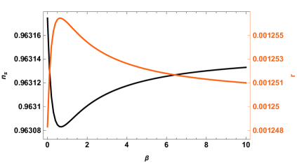
Figure 3: The observations $n_{s}$ vs $r$ locate the $1\sigma$ region of Planck data with fixed $\alpha=1/3.001$ and $N=55$.

From Fig. 2(b), it is evident that the predictions are not significantly influenced by the parameter $\beta$. Hence, we can initially set $\beta=0$ in this subsection. To delve deeper into the dependency on $\beta$, we have also computed the predictions $n_{s}$ and $r$ for the models with fixed $\alpha=1/3.001$, as presented in Fig. 3. As $\beta$ increases, the spectrum index $n_{s}$ exhibits a trend of initially decreasing and then subsequently increasing. Concurrently, the tensor-to-scalar ratio $r$ follows an opposite pattern, first increasing and then decreasing. As $\beta$ continues to rise, both $n_{s}$ and r tend to stabilize, indicating a convergence towards specific values,

$$n_{s}=0.96314~{},~{}~{}r=1.25\times 10^{-3}.$$ (36)

IV.1.2 Trajectory II: $0=x_{m_{1}}<x_{e}<x_{i}<x_{M_{2}}$

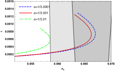
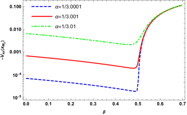
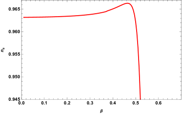
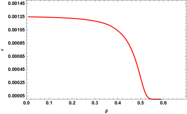
Figure 4: The observations $n_{s}$ vs $r$ (a) and the second-order derivative of potential $V_{xx}(x_{M_{2}})$ (b) for the models with given $\alpha=1/3.0001$ (blue-dashed line), $\alpha=1/3.001$ (red-solid line), and $\alpha=1/3.01$ (green-dot-dashed line). The dependence of $n_{s}$ (c), $r$ (d) on the parameter $\beta$ for the model with $\alpha=1/3.001$ by setting $N=55$.

Setting $\beta=1$, the potential is

$$V(x)=\tanh^{2}\left(\frac{x}{\sqrt{6\alpha}}\right)\left(\tanh\left(\frac{x}{\sqrt{6\alpha}}\right)-1\right)^{2}\text{sech}^{2}\left(\frac{x}{\sqrt{6\alpha}}\right)^{1-3\alpha}$$ (37)

As $\alpha$ approaches $1/3$, the potential undergoes further simplification, resulting in $V\simeq y^{2}(1-y)^{2}$ where $y=\tanh{x/\sqrt{2}}$. This simplified form closely resembles the supersymmetric models discussed in Li et al. (2015), wehich feature a potential of the form $V=|a\phi-b\phi^{2}|^{2}$ with $a,b$ being positive real numbers. However, these models predict a larger value of $r$ than the latest CMB constraints. Conversely, the inflationary models embedded in no-scale supergravity exhibit a value of $r\sim 1\times 10^{-3}$. Setting $N=55$, the numerical results for scalar spectral index $n_{s}$ vs the tensor-to-scalar ratio $r$, second-order derivative of potential $V_{xx}$ for the given value of $\alpha$, as well as the dependence of predictions on $\beta$ are presented in Fig. 4.

As illustrated in Fig. 4(b), the derivative of the potential, $-V_{xx}$, exceeds the value of $0.1$ for models with the parameter $\beta>1$. Consequently, the second slow-roll parameter, $\eta$, falls much below $-0.3$, resulting in the corresponding spectral index, $n_{s}$, falling outside the Planck/BICEP/Keck range. This observation is evident from Fig. 4(c). Therefore, the trajectory form $x_{M_{2}}$ to $x_{m_{1}}(=0)$ is prohibited. Similarly, the inflationary trajectory form $x_{M_{2}}$ to $x_{m_{2}}(>x_{M_{2}})$ follows a comparable pattern. Motivated by the dependence of $V_{xx}$ on the parameter $\beta$, when exploring the viable parameter space for $\beta$ with the condition that $\alpha$ is greater thant $1/3$, for a given value of $\alpha$, it is imperative to identify a suitable $\beta$ that ensures that the absolute value of the second-order derivative of the potential remains below $10^{-2}$.

IV.1.3 Trajectory III: $x_{m_{2}}<x_{e}<x_{i}<x_{M_{3}}$

The last allowable trajectory is from the local maximum $x_{M_{3}}$ to the local minimum $x_{m_{2}}$. The numerical results for scalar spectral index $n_{s}$ vs the tensor-to-scalar ratio $r$ and the dependency of predictions on $\beta$ are presented in Fig. 5. In contrast to models on the previous trajectories, $n_{s}$ or $r$ decreases or increases monotonically with $\beta$.

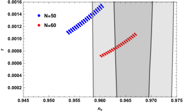
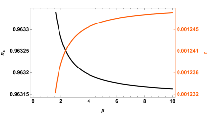
Figure 5: (a) The observations $n_{s}$ vs $r$ for the models with trajectory III. (b) The dependence of $n_{s}$ and $r$ on the parameter $\beta$ for the model with given $\alpha=1/3.001$ and setting $N=55$.

IV.2 $\alpha=1/3$: supersymmetric model with $V=|a\phi-b\phi^{2}|^{2}$

The potential becomes

$$V(x)=\tanh^{2}\left(\frac{x}{\sqrt{2}}\right)\left(1-\beta\tanh\left(\frac{x}{\sqrt{2}}\right)\right)^{2}.$$ (38)

In the limit $x\to\pm\infty$, the potential approaches $(-1\pm\beta)^{2}$, creating a favourable platform for inflation. The plots for the potential with varying $\beta$ are presented in Fig. 6. For models with $0\leq\beta\leq 1/2$, a minimum is located at $x_{m}=0$. Models with $1/2<\beta\leq 1$ exhibit a minimum at $x_{m}=0$ and a maximum locate at $x_{M}=\sqrt{2}\tanh^{-1}\left(\frac{1}{2\beta}\right)$. Finally, for models with $\beta>1$, there are two minima at $x_{m_{1,2}}=0,\sqrt{2}\tanh^{-1}\left(\frac{1}{\beta}\right)$ and a maximum at $x_{M}=\sqrt{2}\tanh^{-1}\left(\frac{1}{2\beta}\right)$. Additionally, the predictions $n_{s}$ vs $r$ for the models are also shown in Fig. 6.

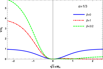
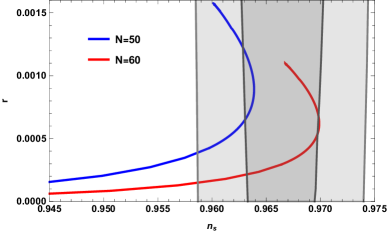
Figure 6: Potential (a) and the predictions $n_{s}$ vs $r$ (b) for the models with $\alpha=1/3$.

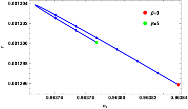
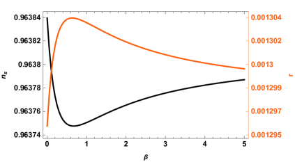
Figure 7: The observations $n_{s}$ vs $r$ for the models with potential (38) and the trajectory is on the regime $x<0$, consistent with the $1\sigma$ region of Planck data by setting $N=55$.

The first slow-roll parameter is

$$\varepsilon(\beta,z)=\frac{\text{csch}^{2}(z)\text{sech}^{2}(z)(\coth(z)-2\beta)^{2}}{(\beta-\coth(z))^{2}}$$ (39)

with $z=x/\sqrt{2}$. The tensor-to-scalar ratio $r=16\varepsilon$ depends on the initial inflation point $x_{i}(z_{i})$ and the parameter $\beta$. By fixing $N=55$, the dependency of $n_{s}$ and $r$ on $\beta$ is depicted in Figs. 7. As the parameter $\beta$ increases, the spectrum index $n_{s}$ initially decreases and then increases, whereas the tensor-to-scalar ratio $r$ first rises and subsequently falls. Eventually, both settle at a particular value.

In the limit $\beta$ approaches infinity and $z_{i}$ is approximately $-3.4~{}M_{\rm Pl}$, the slow-roll parameters are,

$$\begin{split}\varepsilon(z)&\simeq 16\text{csch}^{2}\left(2z\right)\\ &=\frac{64}{(e^{2z}-e^{-2z})^{2}}\simeq 64e^{4z},\\ \eta(z)&\simeq-8\left(\cosh\left(2z\right)-4\right)\text{csch}^{2}\left(2z\right)\\ &=-\frac{16e^{2z}\left(1-8e^{2z}+e^{4z}\right)}{\left(1-e^{4z}\right)^{2}}\simeq-16e^{2z}.\end{split}$$ (40)

Then, the CMB predictions are

$$\begin{split}n_{s}&=1+2\eta-6\varepsilon\simeq 1-32e^{2z}-384e^{4z}\sim 0.9638,\\ r&=16\varepsilon\simeq 1024e^{4z}\sim 1.27\times 10^{-3}.\end{split}$$ (41)

They are consistent with the constraints from Planck and BICEP group, and will be tested by the following QUBIC experiments.

IV.3 $1/3<\alpha<1$

Inspired by the dependence of the predictions $n_{s}$ and $r$ on the parameter $\beta$, we identify parameter space P1 for $\alpha-\beta$ such that the potential fulfills the relations

$$V_{x}(\beta,x)=0~{},~{}~{}V_{xx}(\beta,x)=0~{},~{}~{}\text{with~{}}x>0.$$ (42)

In this manner, the inflationary plateaus emerge naturally, and the predicted observations $n_{s}$ and $r$ are depicted in Fig. 8. The circles, squares, and triangles correspond to the parameter sets $(\alpha,~{}\beta_{1})=(1/3,~{}1/2)$, $(\alpha,~{}\beta_{1})=(2/3,~{}\sqrt{27/32})$, and $(\alpha,~{}\beta_{1})=(1,~{}1)$ respectively. Here, for a given $\alpha$, we denote the corresponding $\beta_{1}$ that satisfies the relations in Eq. (42). Additionally, Fig. 9 displays the corresponding potential and the initial/end points for the inflaton $x$. The non-smooth segment in the figure is attributed to the different inflation-end condition. Specifically, inflation terminates at $\varepsilon=1$ when the model parameter satisfy $\alpha<91/120$. Conversely, for $\alpha>91/120$ inflation ends at $\eta=-1$. This phenomenon is also evident in the $\alpha$-attractor E-Model Lin (2023), where slow-roll inflation ends at $\varepsilon=1$ for models with $\alpha>1/3$ and at $\eta=-1$ for models with $\alpha<1/3$. For the models within the parameter space P1, most predictions of $n_{s}$ fall below the observable values. With $N=60$, the favourable parameter space in P1 is narrow, specifically $1/3\leq\alpha\leq 10027/30000$ as well as $9933/10000\leq\alpha\leq 1$.

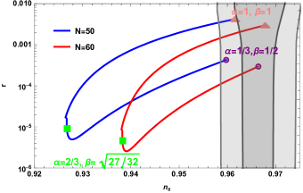
Figure 8: The observations $n_{s}$ vs $r$ (a) for the models with parameter space P1 (b).

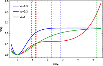
Figure 9: The potential for the models with parameter sets $(\alpha,~{}\beta_{1})=(1/3,~{}1/2)$, $(\alpha,~{}\beta_{1})=(2/3,~{}\sqrt{27/32})$, and $(\alpha,~{}\beta_{1})=(1,~{}1)$ respectively. The vertical lines are the corresponding inflationary initial and end points.

Actually, if we aim to obtain accurate predictions, we need to determine the parameter space P2 for $\alpha-\beta$ to ensure that the potential satisfies the relations,

$$V_{x}(\alpha,\beta,x)\simeq 0~{},~{}~{}V_{xx}(\alpha,\beta,x)=0~{},~{}~{}\text{with~{}}x>0.$$ (43)

We find that a model with $\beta$ slightly smaller than $\beta_{1}$ is capable of yielding cosmological predictions that encompass the entire Planck/BICEP/Keck plane. The results are shown in Fig. 10, featuring eight representative classes of benchmark points for models with $\alpha=1/3,~{}41/120,~{}39/40,~{}2/3,~{}11/12,~{}119/120$ and $1$. Notable, the models with $1/3<\alpha\leq 1$ predict the tensor-to-scalar ratio $r<10^{-3}$, which is compatible with current and future CMB measurements.

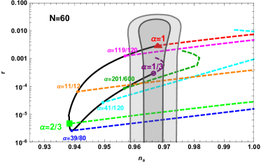
Figure 10: The observations $n_{s}$ vs $r$ for the models with parameter $1/3<\alpha<1$.

V Formation of primordial black holes and scalar-induced gravitational waves

In our recent paper Wu et al. (2021), we have demonstrated that multi-moduli models are more more advantageous than single-modulus models for obtaining broad-band gravitational spectra. Figure 10 illustrates that the models with $\alpha=39/80$ predict the smallest tensor-to-scalar ratio, specifically $r\sim 10^{-5}$. Consequently, in this section, we will delve into the formation of PBHs and SIGWs for the models with $\alpha=39/80$. To introduce an inflection point into the potential, following the approach outlined in Ref. Wu et al. (2021), we incorporate an exponential term $-ae^{-b(\varphi^{2}+\bar{\varphi}^{2})}(\varphi^{2}+\bar{\varphi}^{2})$ into the Kähler potential. Near this inflection point, the potential exhibits a perfect flat plateau, where the slow-roll condition $\eta\ll 1$ is violated, and inflation undergoes an ultra-slow-roll phase. As a result, the power spectrum is significantly enhanced to $\mathcal{O}(10^{-2})$ on small scales.

Model	$\beta$	$a$	$b$	$x_{*}/M_{\rm Pl}$	$n_{s}$	$r$	$N$
M1	0.8181	0.4564032	5.4	2.034	0.9685	$9.1\times 10^{-5}$	51.6
M2	0.8185	0.4528304	5.3	2.035	0.9642	$1.4\times 10^{-4}$	52.7
M3	0.8175	0.450055	5.2	2.041	0.9685	$8.2\times 10^{-4}$	49.2
M4	0.814	0.447051	5.05	2.050	0.9737	$5.3\times 10^{-3}$	56.5

Table 1: The parameters for the model with $\alpha=39/80$ and $c_{1}=1$.

Model	$k/{\rm Mpc}^{-1}$	$\mathcal{P_{R}}$	$M_{pbh}/M_{\odot}$	$f_{pbh}$	$f_{GW}/{\rm Hz}$
M1	$9.6\times 10^{13}$	0.023	$4.0\times 10^{-16}$	0.41	1.1
M2	$2.3\times 10^{12}$	0.025	$7.2\times 10^{-13}$	0.39	0.026
M3	$1.4\times 10^{8}$	0.033	$1.3\times 10^{-4}$	0.068	$1.6\times 10^{-6}$
M4	$1.7\times 10^{5}$	$3.3\times 10^{-3}$	-	-	$1.6\times 10^{-9}$

Table 2: The peak values of the power spectrum, the mass and abundance of PBHs, and the frequency of SIGWs.

Here, we present four benchmark points in Table 1. The parameters are set as $a\sim 0.5$ and $b\sim 5$ to ensure that the additional term can be disregarded, thereby preserving the overall slow-roll story with the exception of introducing an inflection point. The results for $n_{s}$ and $r$ at horizon exit are consistent with the CMB constraints $n_{s}=0.9649\pm 0.0042$ and $r\leq 0.032$ Akrami et al. (2020); Ade et al. (2021). The corresponding peak of power spectrum, the mass and abundance of formed PBHs and the frequency of SIGWs are listed in Table 2.

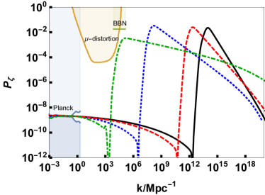
Figure 11: The enhanced scalar power spectrum. The black solid line, red dashed line, blue dotted line, and green dot-dashed line corresponds to the Model M1-M4, respectively. See text for constraint details.

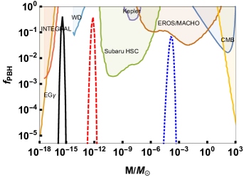
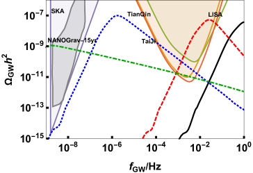
Figure 12: The PBH abundances (a) and the energy densities of SIGWs (b). The black solid line, red dashed line, blue dotted line, and green dot-dashed line corresponds to the Model M1-M4, respectively. See text for constraint details.

We plot the numerical evolution for power spectrum in Fig. 11, the corresponding mass/abundance of PBHs and energy density of SIWGs in Fig. 12. The constraints in these figures are from Ref. Fixsen et al. (1996); Danzmann (1997); Tisserand et al. (2007); Carr et al. (2010); Griest et al. (2013); Moore et al. (2015); Graham et al. (2015); Luo et al. (2016); Inomata et al. (2017); Ali-Haïmoud and Kamionkowski (2017); Poulin et al. (2017); Niikura et al. (2019); Raidal et al. (2017); Ali-Haïmoud et al. (2017); Cai et al. (2019); Hu and Wu (2017); Agazie et al. (2023). The results in figures are distinguished by black solid lines (M1), red dashed lines (M2), blue dotted lines (M3), and green dot-dashed lines (M4). The formed PBHs with masses of $\mathcal{O}(10^{-16}M_{\odot})$ and $\mathcal{O}(10^{-12}M_{\odot})$ can make up all of dark matter, with the abundances approaching $f_{pbh}\simeq 1$. On the other hand, the PBH with mass of $\mathcal{O}(10^{-4}M_{\odot})$ only contribute partially to dark matter with $f_{pbh}\simeq 0.07$. In model M4, a broad-band stochastic gravitational wave background is generated, accounting for a potential source for the NANOGrav 15-year signal Agazie et al. (2023). The SIWGs generated in models M1 and M2 will be probed by the space-based GW detector, such as LISA Danzmann (1997), Taiji Hu and Wu (2017) and TianQin Luo et al. (2016). On the other hand, the SIWGs generated in model M3 will be tested by the future ground-based GW observatories.

VI Conclusion

A novel class of $\alpha$-generalized inflation models has been realized within the framework of no-scale supergravity. The parameter $\alpha$ is constrained to fall within the range of $(0,1]$. The no-scale inflation models, inspired by string compactifications, can be reconstructed by setting values of $\alpha$ for models with one modulus ($\alpha=1$), two moduli ($\alpha=2/3$), and three moduli ($\alpha=1/3$). We have systematically investigated the potential inflationary trajectory and subsequently calculated, both analytically and numerically, the spectrum index $n_{s}$ and tensor-to-scalar ratio $r$. The obtained small value of $r$ is not only consistent with the current observations from Planck/BICEP/Keck Array group, but it is also likely to hold true under future tighter constraints. Notably, the predicted $n_{s}~{}vs~{}r$ in these models covers the whole observed plane. Furthermore, the tensor-to-scalar ratio $r$ can be smaller than $10^{-5}$, making these model particularly suitable for discussing the generation of primordial black holes and scalar-induce gravitational waves.

By incorporating an exponential term into the Kähler potential, an inflection point is introduced into the scalar potential. This addition does not affect the original slow-roll inflation, except for the insertion of an ultra-slow-roll phase. Thus, the power spectrum for the primordial curvature perturbation is significantly enhanced. When the scalar perturbations and tensor perturbations couple at the nonlinear level, large primordial curvature perturbations at small scales induce second-order tensor perturbations. Subsequently, primordial black holes with a wide range of masses are formed, potentially accounting for the entirety or a portion of dark matter. The production of broad-band stochastic gravitational waves is compatible with the observations made by pulsar time array experiments, such as NANOGrav. On the other hand, peak-like gravitational waves will be tested by the upcoming space-based or ground-based gravitational wave observatories.

References

- Starobinsky (1980) A. A. Starobinsky, A New Type of Isotropic Cosmological Models Without Singularity, Phys. Lett. B 91, 99 (1980).
- Guth (1981) A. H. Guth, The Inflationary Universe: A Possible Solution to the Horizon and Flatness Problems, Phys. Rev. D 23, 347 (1981).
- Linde (1982) A. D. Linde, A New Inflationary Universe Scenario: A Possible Solution of the Horizon, Flatness, Homogeneity, Isotropy and Primordial Monopole Problems, Phys. Lett. B 108, 389 (1982).
- Akrami et al. (2020) Y. Akrami et al. (Planck), Planck 2018 results. X. Constraints on inflation, Astron. Astrophys. 641, A10 (2020), arXiv:1807.06211 [astro-ph.CO] .
- Ade et al. (2021) P. A. R. Ade et al. (BICEP, Keck), Improved Constraints on Primordial Gravitational Waves using Planck, WMAP, and BICEP/Keck Observations through the 2018 Observing Season, Phys. Rev. Lett. 127, 151301 (2021), arXiv:2110.00483 [astro-ph.CO] .
- Tristram et al. (2022) M. Tristram et al., Improved limits on the tensor-to-scalar ratio using BICEP and Planck data, Phys. Rev. D 105, 083524 (2022), arXiv:2112.07961 [astro-ph.CO] .
- Allys et al. (2023) E. Allys et al. (LiteBIRD), Probing Cosmic Inflation with the LiteBIRD Cosmic Microwave Background Polarization Survey, PTEP 2023, 042F01 (2023), arXiv:2202.02773 [astro-ph.IM] .
- Ellis et al. (2013a) J. Ellis, D. V. Nanopoulos, and K. A. Olive, No-Scale Supergravity Realization of the Starobinsky Model of Inflation, Phys. Rev. Lett. 111, 111301 (2013a), [Erratum: Phys.Rev.Lett. 111, 129902 (2013)], arXiv:1305.1247 [hep-th] .
- Ellis et al. (2022) J. Ellis, M. A. G. Garcia, D. V. Nanopoulos, K. A. Olive, and S. Verner, BICEP/Keck constraints on attractor models of inflation and reheating, Phys. Rev. D 105, 043504 (2022), arXiv:2112.04466 [hep-ph] .
- Ellis et al. (2013b) J. Ellis, D. V. Nanopoulos, and K. A. Olive, Starobinsky-like Inflationary Models as Avatars of No-Scale Supergravity, J. Cosmol. Astropart. Phys. 10 (2013) 009, arXiv:1307.3537 [hep-th] .
- De Felice et al. (2023) A. De Felice, R. Kawaguchi, K. Mizui, and S. Tsujikawa, Starobinsky inflation with a quadratic Weyl tensor, Phys. Rev. D 108, 123524 (2023), arXiv:2309.01835 [gr-qc] .
- Jeong et al. (2023) H. Jeong, K. Kamada, A. A. Starobinsky, and J. Yokoyama, Reheating process in the R 2 inflationary model with the baryogenesis scenario, J. Cosmol. Astropart. Phys. 11 (2023) 023, arXiv:2305.14273 [hep-ph] .
- Brinkmann et al. (2023) M. Brinkmann, M. Cicoli, and P. Zito, Starobinsky inflation from string theory?, J. High Energ. Phys. 09 (2023) 038, arXiv:2305.05703 [hep-th] .
- Kallosh et al. (2013) R. Kallosh, A. Linde, and D. Roest, Superconformal Inflationary -Attractors, J. High Energ. Phys. 11 (2013) 198, arXiv:1311.0472 [hep-th] .
- Sabir et al. (2020) M. Sabir, W. Ahmed, Y. Gong, and Y. Lu, -attractor from superconformal E-models in brane inflation, Eur. Phys. J. C 80, 15 (2020), arXiv:1903.08435 [gr-qc] .
- Ellis et al. (2019) J. Ellis, D. V. Nanopoulos, K. A. Olive, and S. Verner, Unified No-Scale Attractors, J. Cosmol. Astropart. Phys. 09 (2019) 040, arXiv:1906.10176 [hep-th] .
- Ellis et al. (2020a) J. Ellis, D. V. Nanopoulos, K. A. Olive, and S. Verner, Phenomenology and Cosmology of No-Scale Attractor Models of Inflation, J. Cosmol. Astropart. Phys. 08 (2020) 037, arXiv:2004.00643 [hep-ph] .
- Gao and Gong (2018) Q. Gao and Y. Gong, Reconstruction of extended inflationary potentials for attractors, Eur. Phys. J. Plus 133, 491 (2018), arXiv:1703.02220 [gr-qc] .
- Iacconi et al. (2022) L. Iacconi, H. Assadullahi, M. Fasiello, and D. Wands, Revisiting small-scale fluctuations in -attractor models of inflation, J. Cosmol. Astropart. Phys. 06 (2022) 007, arXiv:2112.05092 [astro-ph.CO] .
- Chen et al. (2020) H.-Y. Chen, I. Gogoladze, S. Hu, T. Li, and L. Wu, Natural Higgs Inflation, Gauge Coupling Unification, and Neutrino Masses, Int. J. Mod. Phys. A 35, 2050117 (2020), arXiv:1805.00161 [hep-ph] .
- Karydas et al. (2021) S. Karydas, E. Papantonopoulos, and E. N. Saridakis, Successful Higgs inflation from combined nonminimal and derivative couplings, Phys. Rev. D 104, 023530 (2021), arXiv:2102.08450 [gr-qc] .
- Shaposhnikov et al. (2021) M. Shaposhnikov, A. Shkerin, I. Timiryasov, and S. Zell, Higgs inflation in Einstein-Cartan gravity, J. Cosmol. Astropart. Phys. 02 (2021) 008, [Erratum: JCAP 10, E01 (2021)], arXiv:2007.14978 [hep-ph] .
- Kallosh and Linde (2022a) R. Kallosh and A. Linde, Polynomial -attractors, J. Cosmol. Astropart. Phys. 04 (2022) 017, arXiv:2202.06492 [astro-ph.CO] .
- Bhattacharya et al. (2023) S. Bhattacharya, K. Dutta, M. R. Gangopadhyay, and A. Maharana, -attractor inflation: Models and predictions, Phys. Rev. D 107, 103530 (2023), arXiv:2212.13363 [astro-ph.CO] .
- Germán (2021) G. Germán, New generalization of the simplest -attractor model, Phys. Rev. D 104, 083015 (2021).
- Linares Cedeño et al. (2023) F. X. Linares Cedeño, G. German, J. C. Hidalgo, and A. Montiel, Bayesian analysis for a class of -attractor inflationary models, J. Cosmol. Astropart. Phys. 03 (2023) 038, arXiv:2212.13610 [astro-ph.CO] .
- Ellis et al. (2016) J. Ellis, M. A. G. Garcia, D. V. Nanopoulos, and K. A. Olive, No-Scale Inflation, Class. Quant. Grav. 33, 094001 (2016), arXiv:1507.02308 [hep-ph] .
- Pallis (2023) C. Pallis, Starobinsky-type B-L Higgs inflation Leading beyond MSSM, PoS CORFU2022, 101 (2023), arXiv:2305.00523 [hep-ph] .
- Ellis et al. (2020b) J. Ellis, M. A. G. Garcia, N. Nagata, N. D. V., K. A. Olive, and S. Verner, Building models of inflation in no-scale supergravity, Int. J. Mod. Phys. D 29, 2030011 (2020b), arXiv:2009.01709 [hep-ph] .
- Wu et al. (2021) L. Wu, Y. Gong, and T. Li, Primordial black holes and secondary gravitational waves from string inspired general no-scale supergravity, Phys. Rev. D 104, 123544 (2021), arXiv:2105.07694 [gr-qc] .
- Wu and Li (2022) L. Wu and T. Li, Generic no-scale inflation inspired from string theory compactifications, Phys. Rev. D 106, 043514 (2022), arXiv:2205.14639 [hep-ph] .
- Wu et al. (2017) L. Wu, S. Hu, and T. Li, No-Scale -Term Hybrid Inflation, Eur. Phys. J. C 77, 168 (2017), arXiv:1605.00735 [hep-ph] .
- Ellis et al. (2018) J. Ellis, M. Fairbairn, A. E. Romano, and O. Zapata, Simple no-scale model of modulus fixing and inflation, Phys. Rev. D 98, 103514 (2018), arXiv:1802.05713 [hep-ph] .
- Li et al. (2015) T. Li, Z. Sun, C. Tian, and L. Wu, The Renormalizable Three-Term Polynomial Inflation with Large Tensor-to-Scalar Ratio, Eur. Phys. J. C 75, 301 (2015), arXiv:1407.8063 [hep-ph] .
- Baumann (2022) D. Baumann, Cosmology (Cambridge University Press, 2022).
- Sasaki (1986) M. Sasaki, Large Scale Quantum Fluctuations in the Inflationary Universe, Prog. Theor. Phys. 76, 1036 (1986).
- Mukhanov (1988) V. F. Mukhanov, Quantum Theory of Gauge Invariant Cosmological Perturbations, Sov. Phys. JETP 67, 1297 (1988).
- Baumann et al. (2019) D. Baumann, H. S. Chia, and R. A. Porto, Probing Ultralight Bosons with Binary Black Holes, Phys. Rev. D 99, 044001 (2019), arXiv:1804.03208 [gr-qc] .
- Tsamis and Woodard (2004) N. C. Tsamis and R. P. Woodard, Improved estimates of cosmological perturbations, Phys. Rev. D 69, 084005 (2004), arXiv:astro-ph/0307463 .
- Kinney (2005) W. H. Kinney, Horizon crossing and inflation with large eta, Phys. Rev. D 72, 023515 (2005), arXiv:gr-qc/0503017 .
- Lin et al. (2020) J. Lin, Q. Gao, Y. Gong, Y. Lu, C. Zhang, and F. Zhang, Primordial black holes and secondary gravitational waves from and inflation, Phys. Rev. D 101, 103515 (2020), arXiv:2001.05909 [gr-qc] .
- Yi et al. (2021) Z. Yi, Q. Gao, Y. Gong, and Z.-h. Zhu, Primordial black holes and scalar-induced secondary gravitational waves from inflationary models with a noncanonical kinetic term, Phys. Rev. D 103, 063534 (2021), arXiv:2011.10606 [astro-ph.CO] .
- Gao et al. (2021) Q. Gao, Y. Gong, and Z. Yi, Primordial black holes and secondary gravitational waves from natural inflation, Nucl. Phys. B 969, 115480 (2021), arXiv:2012.03856 [gr-qc] .
- Lin et al. (2023) J. Lin, S. Gao, Y. Gong, Y. Lu, Z. Wang, and F. Zhang, Primordial black holes and scalar induced gravitational waves from Higgs inflation with noncanonical kinetic term, Phys. Rev. D 107, 043517 (2023), arXiv:2111.01362 [gr-qc] .
- Cai et al. (2023) Y. Cai, M. Zhu, and Y.-S. Piao, Primordial black holes from null energy condition violation during inflation, arXiv:2305.10933 [gr-qc] .
- Wang et al. (2024) Z. Wang, S. Gao, Y. Gong, and Y. Wang, Primordial black holes and scalar-induced gravitational waves from the polynomial attractor model, arXiv:2401.16069 [gr-qc] .
- Lu et al. (2019) Y. Lu, Y. Gong, Z. Yi, and F. Zhang, Constraints on primordial curvature perturbations from primordial black hole dark matter and secondary gravitational waves, J. Cosmol. Astropart. Phys. 12 (2019) 031, arXiv:1907.11896 [gr-qc] .
- Fu et al. (2019) C. Fu, P. Wu, and H. Yu, Primordial Black Holes from Inflation with Nonminimal Derivative Coupling, Phys. Rev. D 100, 063532 (2019), arXiv:1907.05042 [astro-ph.CO] .
- Zhang (2022) F. Zhang, Primordial black holes and scalar induced gravitational waves from the E model with a Gauss-Bonnet term, Phys. Rev. D 105, 063539 (2022), arXiv:2112.10516 [gr-qc] .
- Heydari and Karami (2022) S. Heydari and K. Karami, Primordial black holes ensued from exponential potential and coupling parameter in nonminimal derivative inflation model, J. Cosmol. Astropart. Phys. 03 (2022) 033, arXiv:2111.00494 [gr-qc] .
- Rezazadeh et al. (2022) K. Rezazadeh, Z. Teimoori, S. Karimi, and K. Karami, Non-Gaussianity and secondary gravitational waves from primordial black holes production in -attractor inflation, Eur. Phys. J. C 82, 758 (2022), arXiv:2110.01482 [gr-qc] .
- Ahmed et al. (2022) W. Ahmed, M. Junaid, and U. Zubair, Primordial black holes and gravitational waves in hybrid inflation with chaotic potentials, Nucl. Phys. B 984, 115968 (2022), arXiv:2109.14838 [astro-ph.CO] .
- Spanos and Stamou (2021) V. C. Spanos and I. D. Stamou, Gravitational waves and primordial black holes from supersymmetric hybrid inflation, Phys. Rev. D 104, 123537 (2021), arXiv:2108.05671 [astro-ph.CO] .
- Cai et al. (2021) R.-G. Cai, C. Chen, and C. Fu, Primordial black holes and stochastic gravitational wave background from inflation with a noncanonical spectator field, Phys. Rev. D 104, 083537 (2021), arXiv:2108.03422 [astro-ph.CO] .
- Pi and Wang (2023) S. Pi and J. Wang, Primordial black hole formation in Starobinsky’s linear potential model, J. Cosmol. Astropart. Phys. 06 (2023) 018, arXiv:2209.14183 [astro-ph.CO] .
- Kallosh and Linde (2022b) R. Kallosh and A. Linde, Dilaton-axion inflation with PBHs and GWs, J. Cosmol. Astropart. Phys. 08 (2022) 037, arXiv:2203.10437 [hep-th] .
- Braglia et al. (2023) M. Braglia, A. Linde, R. Kallosh, and F. Finelli, Hybrid -attractors, primordial black holes and gravitational wave backgrounds, J. Cosmol. Astropart. Phys. 04 (2023) 033, arXiv:2211.14262 [astro-ph.CO] .
- Kawai and Kim (2023) S. Kawai and J. Kim, Primordial black holes and gravitational waves from nonminimally coupled supergravity inflation, Phys. Rev. D 107, 043523 (2023), arXiv:2209.15343 [astro-ph.CO] .
- Fu and Chen (2023) C. Fu and C. Chen, Sudden braking and turning with a two-field potential bump: primordial black hole formation, J. Cosmol. Astropart. Phys. 05 (2023) 005, arXiv:2211.11387 [astro-ph.CO] .
- Fu and Wang (2023) C. Fu and S.-J. Wang, Primordial black holes and induced gravitational waves from double-pole inflation, J. Cosmol. Astropart. Phys. 06 (2023) 012, arXiv:2211.03523 [astro-ph.CO] .
- Mavromatos et al. (2022) N. E. Mavromatos, V. C. Spanos, and I. D. Stamou, Primordial black holes and gravitational waves in multiaxion-Chern-Simons inflation, Phys. Rev. D 106, 063532 (2022), arXiv:2206.07963 [hep-th] .
- Yi (2023) Z. Yi, Primordial black holes and scalar-induced gravitational waves from the generalized Brans-Dicke theory, J. Cosmol. Astropart. Phys. 03 (2023) 048, arXiv:2206.01039 [gr-qc] .
- Meng et al. (2023) D.-S. Meng, C. Yuan, and Q.-G. Huang, Primordial black holes generated by the non-minimal spectator field, Sci. China Phys. Mech. Astron. 66, 280411 (2023), arXiv:2212.03577 [astro-ph.CO] .
- Qiu et al. (2023) T. Qiu, W. Wang, and R. Zheng, Generation of primordial black holes from an inflation model with modified dispersion relation, Phys. Rev. D 107, 083018 (2023), arXiv:2212.03403 [astro-ph.CO] .
- Mu et al. (2023a) B. Mu, G. Cheng, J. Liu, and Z.-K. Guo, Constraints on ultraslow-roll inflation from the third LIGO-Virgo observing run, Phys. Rev. D 107, 043528 (2023a), arXiv:2211.05386 [astro-ph.CO] .
- Mu et al. (2023b) B. Mu, J. Liu, G. Cheng, and Z.-K. Guo, Constraints on ultra-slow-roll inflation with the NANOGrav 15-Year Dataset, arXiv:2310.20564 [astro-ph.CO] .
- Poisson et al. (2023) A. Poisson, I. Timiryasov, and S. Zell, Critical Points in Palatini Higgs Inflation with Small Non-Minimal Coupling, arXiv:2306.03893 [hep-ph] .
- Heydari and Karami (2024) S. Heydari and K. Karami, Primordial black holes and secondary gravitational waves from generalized power-law non-canonical inflation with quartic potential, Eur. Phys. J. C 84, 127 (2024), arXiv:2310.11030 [gr-qc] .
- Ghoshal et al. (2023) A. Ghoshal, A. Moursy, and Q. Shafi, Cosmological probes of grand unification: Primordial black holes and scalar-induced gravitational waves, Phys. Rev. D 108, 055039 (2023), arXiv:2306.04002 [hep-ph] .
- Zhao et al. (2023) J.-X. Zhao, X.-H. Liu, and N. Li, Primordial black holes and scalar-induced gravitational waves from the perturbations on the inflaton potential in peak theory, Phys. Rev. D 107, 043515 (2023), arXiv:2302.06886 [astro-ph.CO] .
- Arya et al. (2024) R. Arya, R. K. Jain, and A. K. Mishra, Primordial black holes dark matter and secondary gravitational waves from warm Higgs-G inflation, J. Cosmol. Astropart. Phys. 02 (2024) 034, arXiv:2302.08940 [astro-ph.CO] .
- Solbi and Karami (2024) M. Solbi and K. Karami, Primordial black holes in non-minimal coupling Gauss-Bonnet inflation in light of the NANOGrav 15 year data, arXiv:2403.00021 [gr-qc] .
- Chen et al. (2024) L.-Y. Chen, H. Yu, and P. Wu, Resonant amplification of curvature perturbations in inflation model with periodical derivative coupling, Phys. Lett. B 849, 138457 (2024), arXiv:2401.07523 [gr-qc] .
- Zhao and Li (2024) J.-X. Zhao and N. Li, An analytical approximation of the evolution of the primordial curvature perturbation in the ultraslow-roll inflation: an extended study, Eur. Phys. J. C 84, 222 (2024), arXiv:2403.01416 [astro-ph.CO] .
- Gao et al. (2024) T.-J. Gao, K.-S. Sun, and X.-Y. Yang, Nanohertz gravitational waves from supergravity inflationary model with double-inflection-point, Eur. Phys. J. C 84, 188 (2024).
- Lin (2023) C.-M. Lin, The average equation of state for the oscillating inflaton field of the simplest -attractor E-model, arXiv:2305.01159 [hep-ph] .
- Fixsen et al. (1996) D. J. Fixsen, E. S. Cheng, J. M. Gales, J. C. Mather, R. A. Shafer, and E. L. Wright, The Cosmic Microwave Background spectrum from the full COBE FIRAS data set, Astrophys. J. 473, 576 (1996), arXiv:astro-ph/9605054 .
- Danzmann (1997) K. Danzmann, LISA: An ESA cornerstone mission for a gravitational wave observatory, Class. Quant. Grav. 14, 1399 (1997).
- Tisserand et al. (2007) P. Tisserand et al. (EROS-2), Limits on the Macho Content of the Galactic Halo from the EROS-2 Survey of the Magellanic Clouds, Astron. Astrophys. 469, 387 (2007), arXiv:astro-ph/0607207 .
- Carr et al. (2010) B. J. Carr, K. Kohri, Y. Sendouda, and J. Yokoyama, New cosmological constraints on primordial black holes, Phys. Rev. D 81, 104019 (2010), arXiv:0912.5297 [astro-ph.CO] .
- Griest et al. (2013) K. Griest, A. M. Cieplak, and M. J. Lehner, New Limits on Primordial Black Hole Dark Matter from an Analysis of Kepler Source Microlensing Data, Phys. Rev. Lett. 111, 181302 (2013).
- Moore et al. (2015) C. J. Moore, R. H. Cole, and C. P. L. Berry, Gravitational-wave sensitivity curves, Class. Quant. Grav. 32, 015014 (2015), arXiv:1408.0740 [gr-qc] .
- Graham et al. (2015) P. W. Graham, S. Rajendran, and J. Varela, Dark Matter Triggers of Supernovae, Phys. Rev. D 92, 063007 (2015), arXiv:1505.04444 [hep-ph] .
- Luo et al. (2016) J. Luo et al. (TianQin), TianQin: a space-borne gravitational wave detector, Class. Quant. Grav. 33, 035010 (2016), arXiv:1512.02076 [astro-ph.IM] .
- Inomata et al. (2017) K. Inomata, M. Kawasaki, K. Mukaida, Y. Tada, and T. T. Yanagida, Inflationary primordial black holes for the LIGO gravitational wave events and pulsar timing array experiments, Phys. Rev. D 95, 123510 (2017), arXiv:1611.06130 [astro-ph.CO] .
- Ali-Haïmoud and Kamionkowski (2017) Y. Ali-Haïmoud and M. Kamionkowski, Cosmic microwave background limits on accreting primordial black holes, Phys. Rev. D 95, 043534 (2017), arXiv:1612.05644 [astro-ph.CO] .
- Poulin et al. (2017) V. Poulin, P. D. Serpico, F. Calore, S. Clesse, and K. Kohri, CMB bounds on disk-accreting massive primordial black holes, Phys. Rev. D 96, 083524 (2017), arXiv:1707.04206 [astro-ph.CO] .
- Niikura et al. (2019) H. Niikura et al., Microlensing constraints on primordial black holes with Subaru/HSC Andromeda observations, Nature Astron. 3, 524 (2019), arXiv:1701.02151 [astro-ph.CO] .
- Raidal et al. (2017) M. Raidal, V. Vaskonen, and H. Veermäe, Gravitational Waves from Primordial Black Hole Mergers, J. Cosmol. Astropart. Phys. 09 (2017) 037, arXiv:1707.01480 [astro-ph.CO] .
- Ali-Haïmoud et al. (2017) Y. Ali-Haïmoud, E. D. Kovetz, and M. Kamionkowski, Merger rate of primordial black-hole binaries, Phys. Rev. D 96, 123523 (2017), arXiv:1709.06576 [astro-ph.CO] .
- Cai et al. (2019) R.-G. Cai, S. Pi, S.-J. Wang, and X.-Y. Yang, Resonant multiple peaks in the induced gravitational waves, J. Cosmol. Astropart. Phys. 05 (2019) 013, arXiv:1901.10152 [astro-ph.CO] .
- Hu and Wu (2017) W.-R. Hu and Y.-L. Wu, The Taiji Program in Space for gravitational wave physics and the nature of gravity, Natl. Sci. Rev. 4, 685 (2017).
- Agazie et al. (2023) G. Agazie et al. (NANOGrav), The NANOGrav 15 yr Data Set: Evidence for a Gravitational-wave Background, Astrophys. J. Lett. 951, L8 (2023), arXiv:2306.16213 [astro-ph.HE] .