Satisfiability to Coverage in Presence of Fairness, Matroid, and Global Constraints

Abstract

In the MaxSAT with Cardinality Constraint problem (CC-MaxSAT), we are given a CNF-formula $\Phi$, and a positive integer $k$, and the goal is to find an assignment $\beta$ with at most $k$ variables set to true (also called a weight $k$-assignment) such that the number of clauses satisfied by $\beta$ is maximized. Maximum Coverage can be seen as a special case of CC-MaxSat, where the formula $\Phi$ is monotone, i.e., does not contain any negative literals. CC-MaxSat and Maximum Coverage are extremely well-studied problems in the approximation algorithms as well as parameterized complexity literature.

Our first conceptual contribution is that CC-MaxSat and Maximum Coverage are equivalent to each other in the context of FPT-Approximation parameterized by $k$ (here, the approximation is in terms of number of clauses satisfied/elements covered). In particular, we give a randomized reduction from CC-MaxSat to Maximum Coverage running in time $\mathcal{O}(1/\epsilon)^{k}\cdot(m+n)^{\mathcal{O}(1)}$ that preserves the approximation guarantee up to a factor of $1-\epsilon$. Furthermore, this reduction also works in the presence of ``fairness'' constraints on the satisfied clauses, as well as matroid constraints on the set of variables that are assigned $\mathsf{true}$. Here, the ``fairness'' constraints are modeled by partitioning the clauses of the formula $\Phi$ into $r$ different colors, and the goal is to find an assignment that satisfies at least $t_{j}$ clauses of each color $1\leq j\leq r$.

Armed with this reduction, we focus on designing FPT-Approximation schemes (FPT-ASes) for Maximum Coverage and its generalizations. Our algorithms are based on a novel combination of a variety of ideas, including a carefully designed probability distribution that exploits sparse coverage functions. These algorithms substantially generalize the results in Jain et al. [SODA 2023] for CC-MaxSat and Maximum Coverage for $K_{d,d}$-free set systems (i.e., no $d$ sets share $d$ elements), as well as a recent FPT-AS for Matroid Constrained Maximum Coverage by Sellier [ESA 2023] for frequency-$d$ set systems.

1 Introduction

Two problems that have gained considerable attention from the perspective of Parameterized Approximation [12] are the classical MaxSAT with cardinality constraint (CC-MaxSat) problem and its monotone version, the Maximum Coverage problem. In the CC-MaxSat problem, we are given a CNF-formula $\Phi$ over $m$ clauses and $n$ variables, and a positive integer $k$, and the objective is to find a weight $k$ assignment that maximizes the number of satisfied clauses. We use ${\sf var}(\Phi)$ and ${\sf cla}(\Phi)$ to denote the set of variables and clauses in $\Phi$, respectively. An assignment to a CNF-formula $\Phi$ is a function $\beta:{\sf var}(\Phi)\rightarrow\{0,1\}$. The weight of an assignment $\beta$ is the number of variables that have been assigned $1$.

The classical Maximum Coverage problem is a special case of the CC-MaxSat problem. Indeed, it is a monotone variant of CC-MaxSat, where negated literals are not allowed. An input to the Maximum Coverage problem consists of a family of $m$ sets, $\cal F$, over a universe $U$ of size $n$, and an integer $k$, and the goal is to find a subfamily ${\cal F}^{\prime}\subseteq{\cal F}$ of size $k$ such that the number of elements covered (belongs to some set in ${\cal F}^{\prime}$) by ${\cal F}^{\prime}$ is maximized. Observe that when the goal is to cover every element in $U$, the Maximum Coverage problem corresponds to Set Cover. A natural question that has guided research on these problems is whether CC-MaxSat or Maximum Coverage admits an algorithm with running time $f(k)n^{{\mathcal{O}}(1)}$? That is, whether CC-MaxSat or Maximum Coverage is fixed parameter tractable (FPT) with solution size $k$? Unfortunately, these problems are W[2]-hard [10]. That is, we do not expect these problems to admit an algorithm with running time $f(k)n^{{\mathcal{O}}(1)}$. This negative result sets the platform for studying these problems from the viewpoint of Parameterized Approximation [12]. It is well known that both CC-MaxSat and Maximum Coverage admit a polynomial time $(1-\frac{1}{e})$-approximation algorithm [28], which is in fact optimal. [11]. So, in the realm of Parameterized Approximation, we ask does there exist an $\epsilon>0$, such that CC-MaxSat or Maximum Coverage admits an approximation algorithm with factor $(1-\frac{1}{e}+\epsilon)$ and runs in time $f(k,\epsilon)n^{{\mathcal{O}}(1)}$. While there has been a lot of work on Maximum Coverage [18, 22, 27, 16, 26], Jain et al. [18] studied CC-MaxSat and designed a standalone algorithm for the problem. Our first result, a bit of a surprise to us, shows that in the world of Parameterized Approximation CC-MaxSat and Maximum Coverage are ``equivalent".

Theorem 1.1 (Informal).

Let $\epsilon>0$. There is a polynomial time randomized algorithm that given an instance $(\Phi,k)$ of CC-MaxSat produces an instance $(U,{\cal F},k)$ of Maximum Coverage such that the following holds with probability $\frac{1}{2}(\frac{\epsilon}{2})^{k}$. Given a $(1-\epsilon){\sf OPT_{cov}}$ solution to $(U,{\cal F},k)$ we can obtain a $(1-\epsilon){\sf OPT_{sat}}$ solution to $(\Phi,k)$ in polynomial time. Here, ${\sf OPT_{cov}}$ (${\sf OPT_{sat}}$) denotes the value of the maximum number of covered elements (satisfied clauses) by a $k$ sized family of subsets (weight $k$ assignment).

Theorem 1.1 allows us to focus on Maximum Coverage, rather than CC-MaxSat, at the expense of $\epsilon^{-\mathcal{O}(k)}$ in the running time. Further, there is no assumption on the input formulas in Theorem 1.1. This reduction immediately implies faster algorithms for CC-MaxSat by utilizing the known good algorithms for Maximum Coverage [18, 22, 27, 16, 26]. The Maximum Coverage problem has been generalized in several directions by adding either fairness constraints or asking our solution to be an independent set of a matroid. In what follows, we take a closer look at progresses on Maximum Coverage and its generalizations and then design algorithms that generalize and unify all the known results for CC-MaxSat and Maximum Coverage.

1.1 Tractability Boundaries for Maximum Coverage

Cohen-Addad et al. [9] studied Maximum Coverage and showed that there is no $\epsilon>0$, such that Maximum Coverage admits an approximation algorithm with factor $(1-\frac{1}{e}+\epsilon)$ and runs in time $f(k,\epsilon)(m+n)^{{\mathcal{O}}(1)}$ . Later, this was also studied by Manurangsi [22], who obtained the following strengthening over [9]: for any constant $\epsilon>0$ and any function $h$, assuming Gap-ETH, no $h(k)(n+m)^{o(k)}$ time algorithm can approximate Maximum Coverage with $n$ elements and $m$ sets to within a factor $(1-\frac{1}{e}+\epsilon)$, even with a promise that there exist $k$ sets that fully cover the whole universe. This negative result sets the contour for possible positive results. In particular, if we hope for an FPT algorithm that improves over a factor $(1-\frac{1}{e})$ then we must assume some additional structure on the input families. This automatically leads to the families wherein each set has bounded size, or each element appears in bounded sets which was considered earlier.

Skowron and Faliszewski [27] showed that, if we are working on set families, such that each element in $U$ appears in at most $p$ sets, then there exists an algorithm, that given an $\epsilon>0$, runs in time $(\frac{p}{\epsilon})^{{\mathcal{O}}(k)}n^{{\mathcal{O}}(1)}$ and returns a subfamily ${\cal F}^{\prime}$ of size $k$ that is a $(1-\epsilon)$-approximation. These kind of FPT-approximation algorithms are called FPT-approximation Schemes (FPT-ASes). For $p=2$, Manurangsi [22] independently obtained a similar result. Jain et al. [18] generalized these two settings by looking at $K_{d,d}$-free set systems (i.e., no $d$ sets share $d$ elements). They also considered $K_{d,d}$-free formulas (that is, the clause-variable incidence bipartite graph of the formula excludes $K_{d,d}$ as an induced subgraph). They showed that for every $\epsilon>0$, there exists an algorithm for $K_{d,d}$-free formulas with approximation ratio $(1-\epsilon)$ and running in time $2^{\mathcal{O}((\frac{dk}{\epsilon})^{d})}(n+m)^{\mathcal{O}(1)}$. For, Maximum Coverage on $K_{d,d}$-free set families, they obtain an FPT-AS with running time $(\frac{dk}{\epsilon})^{\mathcal{O}(dk)}n^{\mathcal{O}(1)}$. Using these results together with Theorem 1.1 we get the following.

Corollary 1.2.

Let $\epsilon>0$. Then, CC-MaxSat admits a randomized FPT-AS with running time $(\frac{dk}{\epsilon})^{\mathcal{O}(dk)}n^{\mathcal{O}(1)}$ on $K_{d,d}$-free formulas. Furthermore, if the size of clauses is bounded by $p$ or every variable appears in at most $p$ clauses then CC-MaxSat admits randomized FPT-AS with running time $(\frac{p}{\epsilon})^{{\mathcal{O}}(k)}n^{{\mathcal{O}}(1)}$. Both results hold with constant probability.

Corollary 1.2 follows by utilizing Theorem 1.1 and repurposing the known results about Maximum Coverage ([18, 6, 27, 22]). We will return to the case of $K_{d,d}$-free set systems later. Apart from extending the classes of set families where Maximum Coverage admits FPT-ASes, the study on the Maximum Coverage problem has been extended in many directions.

1.1.1 Matroid Constraints

Note that Maximum Coverage is a special case of submodular function maximization subject to a cardinality constraint. In the latter problem, we are given (an oracle access to) a submodular function $f:2^{V}\to\mathbb{R}_{\geq 0}$ , and the goal is to find a subset $U\subseteq V$ that maximizes $f(U)$ over all subsets of size at most $k$. Indeed, coverage functions are submodular and monotone (i.e., adding more sets cannot decrease the number of elements covered). There has been a plethora of work on monotone submodular maximization subject to cardinality constraints, starting from Wolsey [29]. In a further generalization, we are interested in monotone submodular maximization subject to a matroid constraint – in this setting, we are given a matroid $\mathcal{M}=(U,\mathcal{I})$ via an independence oracle, i.e., an algorithm that answers queries of the form ``Is $P\in\mathcal{I}$?'' for any $P\subseteq U$ in one step, and we want to find an independent set $S\in I$ that maximizes $f(S)$. Note here that a uniform matroid of rank $k$ exactly captures the cardinality constraint. Calinescu et al. [7] gave an optimal $(1-1/e)$-approximation.

More recently, Huang and Sellier [16] and Sellier [26] studied the problem of maximizing a coverage function subject to a matroid constraint, called Matroid Constrained Maximum Coverage. In this problem, which we call M-MaxCov (M for ``matroid'' constraint), we are given a set system $(U,\mathcal{F})$ and a matroid $\mathcal{M}=(\mathcal{F},I)$ of rank $k$, and the goal is to find a subset $\mathcal{F}^{\prime}\subseteq\mathcal{F}$ such that $\mathcal{F}^{\prime}\in I$ and $\mathcal{F}^{\prime}$ maximizes the number of elements covered. Note that M-MaxCov is a generalization of Maximum Coverage. In the latter paper, Sellier [26] designed an FPT-AS for M-MaxCov, running in time $(d/\epsilon)^{\mathcal{O}(k)}\cdot(m+n)^{\mathcal{O}(1)}$ for frequency-$d$ set systems. Note that this result generalizes that of [27, 22] from a uniform matroid consraint to an arbitrary matroid constraint of rank $k$.

Analogous to M-MaxCov, one can define a matroid constrained version of CC-MaxSat, called M-MaxSAT. In this problem, we are given a CNF-SAT formula $\Phi$ and a matroid $\mathcal{M}$ of rank $k$ on the set of variables. The goal is to find an assignment that satisfies the maximum number of clauses, with the restriction that, the set of variables assigned $1$ must be an independent set in $\mathcal{M}$. Note that M-MaxSAT generalizes M-MaxCov as well as CC-MaxSat. We obtain the following result for M-MaxSAT, by combining the results on a variant of Theorem 1.1 with the corresponding result on M-MaxCov.

Theorem 1.3.

There exists an FPT-AS for M-MaxSAT parameterized by $k,d$, and $\epsilon$, on $d$-CNF formulas, where $k$ denotes the rank of the given matroid.

1.1.2 Fairness or Multiple Coverage Constraints

Now we consider an orthogonal generalization of Maximum Coverage. Note that an optimal solution for Maximum Coverage may leave many elements uncovered. However, such a solution may be deemed unfair if the elements are divided into multiple colors (representing, say, people of different demographic groups), and the set uncovered elements are biased against a specific color. To address these constraints, the following generalization of Maximum Coverage, which we call F-MaxCov (F stands for ``fair''), has been studied in the literature. Here, we are given a set system $(U,\mathcal{F})$, a coloring function $\chi:U\rightarrow[r]$, a coverage requirement function $t:[r]\rightarrow\mathbb{N}$, and an integer $k$; and the goal is to find a subset $\mathcal{F}^{\prime}\subseteq\mathcal{F}$ of size at most $k$ such that, for each $i\in[r]$, the union of elements in $\mathcal{F}^{\prime}$ is at least $t(i)$ (or $t_{i}$).

Since F-MaxCov is a generalisation of Maximum Coverage, it inherits all the lower bounds known for Maximum Coverage. Furthermore, we can mimic the algorithm for Maximum Coverage (Partial Set Cover) parameterized by $t$ (where you want to cover at least $t$ elements with $k$ sets) [6] to obtain an algorithm for Partition Maximum Coverage parameterized by $\sum_{j\in[r]}t_{j}$. However, the problem is NP-hard even when $t_{j}\leq 1$, $j\in[r]$, via a simple reduction from Set Cover.

F-MaxCov has been studied under multiple names in the approximation algorithms literature; however much of the focus has been on approximating the size of the solution, rather than the coverage. Notable exception include Chekuri et al. [8] who gave a ``bicriteria'' approximation, that outputs a solution of size at most $\mathcal{O}(\nicefrac{{\log r}}{{\epsilon}})$ times the optimal size, and covers at least $(1-\nicefrac{{1}}{{e}}-\epsilon)$ fraction of the required coverage of each color. Very recently, Bandyapadhyay et al. [4] recently designed an FPT-AS for F-MaxCov for the set systems of frequency $2$, running in time $2^{\mathcal{O}(\frac{rk^{2}\log k}{\epsilon})}\cdot(m+n)^{\mathcal{O}(1)}$. We obtain the following result on F-MaxCov.

Theorem 1.4.

There exists a randomized FPT-AS for F-MaxCov running in time $\left(dr\left(\frac{\log k}{\epsilon}\right)^{r}\right)^{\mathcal{O}(k)}\cdot(m+n)^{\mathcal{O}(1)}$, on set systems with frequency bounded by $d$.

Note that this result generalizes the result of [4] to frequency-$d$ set systems, and in the case of $d=2$, our running time is faster than that of [4] (albeit our algorithm is randomized).

One can also define fair version of CC-MaxSat in an analogous way, which we call F-MaxSAT. In this problem, we are given a CNF-formula $\Phi$, a coloring function $\chi:{\sf cla}(\Phi)\rightarrow[r]$, a coverage demand function $t:[r]\rightarrow\mathbb{N}$, and an integer $k$. The goal is to find a weight-$k$ assignment that satisfies at least $t(j)$ (also denoted as $t_{j}$) clauses of each color $j\in[r]$. By combining Theorem 1.4 with a slightly more general version of the reduction theorem (Theorem 1.1) also yields FPT-AS for F-MaxSAT with a similar running time.

1.2 Our New Problem: Combining Matroid and Fairness Constraints

As discussed in the previous subsections, Maximum Coverage has been generalized in two orthogonal directions, namely, matroid constraints on the sets chosen in the solution, and fairness constraints on the elements covered by the solution. Although the corresponding variants of CC-MaxSat have not been studied in the literature, we mentioned that our techniques readily imply FPT-ASes for these problems for many ``sparse'' formulas. Given this, the following natural question arises.

In the following, we formally define the common generalization of M-MaxSAT and F-MaxSAT, which we call (M, F)-MaxSAT.

In the special case where the CNF-SAT formula is monotone (i.e., does not contain negated literals), we obtain (M, F)-MaxCov, which generalizes all the variants of Maximum Coverage discussed earlier. We obtain the following result for (M, F)-MaxCov.

Theorem 1.5.

There exists a randomized FPT-AS for (M, F)-MaxCov on set systems with maximum frequency $d$, that runs in time $\left(\frac{d\log k}{\epsilon}\right)^{\mathcal{O}(kr)}\cdot(m+n)^{\mathcal{O}(1)}$ and returns a $(1-\epsilon)$-approximation with at least a constant probability.

Finally, by reducing (M, F)-MaxSAT on $d$-CNF formulas to (M, F)-MaxCov with frequency $d$ set systems, using the randomized reduction, and then using the results of Theorem 1.5, we obtain our most general result, as follows.

Theorem 1.6.

There exists a randomized FPT-AS for (M, F)-MaxSAT on $d$-CNF formulas, that runs in time $\left(\frac{d\log k}{\epsilon}\right)^{\mathcal{O}(kr)}\cdot(m+n)^{\mathcal{O}(1)}$ and returns a $(1-\epsilon)$-approximation with at least a constant probability.

We give a summary of how the various problems are related to each other, and a comparison of our results with the literature in Figure 1.

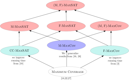
Figure 1: If there is an arrow of the form $A\rightarrow B$, then problem $B$ generalizes problem $A$. FPT-ASes for the problems in red bubbles are not known in the literature, and we study in this paper. For all the other problems FPT-ASes are known in the literature for some cases. This paper improves the results in cyan and blue.

1.3 Related Results

Max $k$-VC or Partial Vertex Cover has been extensively studied in Parameterized Complexity. In this problem we are given a graph and the task is to select a subset of $k$ vertices covering as many of the edges as possible. The problem is known to be approximable within $0.929$ and is hard to approximate within $0.944$, assuming UGC [22]. Max $k$-VC is known to be W[1]-hard [15], parameterized by $k$, but admits FPT algorithms on planar graphs, graphs of bounded degeneracy, $K_{d,d}$-free graphs, and bipartite graphs, parameterized by $k$ [2, 13, 19]. Indeed, it is among the first problems to admit FPT-AS [24, 22, 27]. It is also known to have ``lossy kernels'' [24, 21], a lossy version of classical kernelization.

Bera et al. [5] considered the special case of Partition Vertex Cover, where the set of edges of a graph are divided into $r$ colors, and we want to find a subset of vertices that covers at least a certain number of edges from each color class. For this problem, they gave a polynomial-time $\mathcal{O}(\log r)$-approximation algorithm. Hung and Kao [17] generalized this to F-MaxCov, and gave a $\mathcal{O}(d\log r)$-approximation, where each element of the universe is contained in at most $d$ sets (i.e., $d$ is the maximum frequency). Bandyapadhyay et al. [3] studied this problem under the name of Fair Covering, and designed a $\mathcal{O}(d)$-approximation, but their running time is XP in the number of colors. Chekuri et al. [8] designed a general framework for F-MaxCov, yielding tight approximation guarantees for a variety of set systems satisfying certain property; in particular, they improve the approximation guarantee for frequency-$d$ set systems to $\mathcal{O}(d+\log r)$, which is tight in polynomial time.

2 Overview of Our Results and Techniques

2.1 Reduction from CC-MaxSat to Maximum Coverage: An overview of Theorem 1.1

This theorem is essentially a randomized approximation-preserving reduction from CC-MaxSat to Maximum Coverage. Given an instance $\mathcal{I}=(\Phi,k)$ of CC-MaxSat, we first compute a random assignment $\Psi$ that assigns a variable independently to be $1$ with probability $p=\epsilon/2$ and $0$ with probability $1-p$. Let $V^{*}$ be the set of at most $k$ variables set to be $1$ by an optimal assignment $\Psi^{*}$. It is straightforward to see that, the probability that all the variables in $V^{*}$ are set to be $1$ by the random assignment $\Psi$ is $p^{k}$ – we say that this is the good event $\mathcal{G}$. Now, consider a clause that is satisfied negatively by $\Psi^{*}$, i.e., a clause $C$ that contains a negative literal $\neg x$ and $\Psi^{*}(x)=0$. It is also easy to see that, conditioned on the good event $\mathcal{G}$, the probability that such a clause $C$ is also satisfied negatively by $\Psi$ is at least $1-p$. Thus, the expected number of clauses that are satisfied negatively by $\Psi$, conditioned on $\mathcal{G}$, is at least $1-p$ times the number of clauses satisfied negatively by $\Psi^{*}$. Markov's inequality implies that, with probability at least $1/2$, the actual number of such clauses is close to its expected value. Thus, conditioned on $\mathcal{G}$, and the previous event, we can focus on the positively satisfied clauses (note that the probability that both of these events occur is at least $1/2\cdot(\epsilon/2)^{k}$. To this end, we can eliminate all the negatively satisfied clauses, and we can also prune the remaining clauses by eliminating any negative literals and the variables that are set to $0$ by $\Psi$. Thus, all the remaining clauses only contain positive literals, which can be seen as an instance $\mathcal{I}^{\prime}$ of Maximum Coverage. Furthermore, conditioned on $\mathcal{G}$, the variables set to $1$ by $\Phi^{*}$ correspond to a family $\mathcal{F}^{*}$ of size $k$, and the elements covered by $\mathcal{F}^{*}$ correspond to the set of clauses satisfied only positively by $\Phi^{*}$. Thus, if we find a $(1-\epsilon)$-approximate solution to $\mathcal{I}^{\prime}$, and set the corresponding variables to $1$, and the rest of the variables to $0$, then we get a weight-$k$ assignment that satisfies at least $(1-\epsilon)\cdot\textsf{OPT}_{sat}$ clauses. Note that this reduction, combined with the algorithm of [18] gives the proof of Corollary 1.2.

Furthermore, this reduction is robust enough that it can accommodate the fairness constraints on the clauses, as defined above. To be precise, one can give a similar reduction from $\mathcal{C}$-MaxSAT to $\mathcal{C}$-MaxCov, where $\mathcal{C}\in\left\{\textsc{M, F, (M, F)}\right\}$ – note that when we have fairness constraints, the success probability now becomes $(r/\epsilon)^{\mathcal{O}(k)}$. Essentially, these reductions translate a constraint on the variables set to $1$ (for CC-MaxSat and variants), to the corresponding family of sets (for Maximum Coverage and variants). Thus, at the expense of a multiplicative $(r/\epsilon)^{\mathcal{O}(k)}$ factor in the running time, we can focus on Maximum Coverage and its variants, which is what we do in this section, as well as in the paper. As a warm-up, we start in Section 2.2 with the vanilla Maximum Coverage on frequency-$d$ set systems (where our algorithms do not improve over the known algorithms in the literature), and give a complete formal proof. Then, we will gradually introduce the ideas required to handle fairness (Section 2.3) and matroid (Section 2.4) constraints – first separately, and then together. Finally, in Section 2.5, we briefly discuss the ideas required to these results to $K_{d,d}$-free set systems and multiple matroid constraints.

2.2 Deterministic and Randomized Branching using a Largest Set

To introduce our ideas in a clean and gradual way, we start with the simplest setting of Maximum Coverage where the maximum frequency of the elements is bounded by $d$. Recall that we are given an instance $(U,\mathcal{F},k)$ and the goal is to find a sub-family of $\mathcal{F}$ of size $k$ that covers the maximum number of elements. For any sub-family $\mathcal{R}\subseteq\mathcal{F}$, let $U(\mathcal{R})$ denote the subset of elements covered by $\mathcal{R}$, and $\textsf{OPT}_{k}(\mathcal{R})$ denote the maximum number of elements that can be covered by a subset of $\mathcal{R}$ of size $k$. Further, for a set $S\in\mathcal{F}$, we denote by $\mathcal{F}-S$, the family obtained by removing $S$, as well as the elements of $S$ from each of the remaining sets. Our approach is inspired by the approaches of Skowron and Faliszewski [27] and Manurangsi [22] who show that $\mathcal{O}(kd/\epsilon)$ sets of the largest size is guaranteed to contain a $(1-\epsilon)$-approximate solution. This naturally begs the question, ``why not start by adding the largest set into the solution?'' (in a sense, the following presentation is closer in spirit to Jain et al. [18].) Let us inspect this question more closely. Let $L$ be a largest set in $\mathcal{F}$. By looking at the contribution of coverage of each set in an optimal solution, say $\mathcal{O}$, we can easily see that $|L|\geq\frac{\textsf{OPT}_{k}(\mathcal{F})}{k}$. We say that a set $S\in\mathcal{F}$ is heavy w.r.t. $L$ if $|L\cap S|\geq\frac{\epsilon|L|}{k}$ (note that $L$ is heavy w.r.t. itself). However, since the frequency of each element is bounded by $d$, each element in $L$ can appear in at most $d$ (in fact, $d-1$) sets $L\cap S$ for different $R\in\mathcal{F}$. This implies that at most $\frac{kd}{\epsilon}$ sets in $\mathcal{F}$ are heavy w.r.t. $L$.

Algorithm. Our algorithm simply branches on the sets in $\mathcal{H}(L)$, which is the family of heavy sets w.r.t. $L$. Specifically, in the branch corresponding to a heavy set $S\in\mathcal{H}(L)$, we include it in the solution, and recursively call the algorithm on the residual instance $(U\setminus S,\mathcal{F}-S,k-1)$. If any of the sets in $\mathcal{O}$ is heavy w.r.t. $L$, then in the branch corresponding to such a set yields an approximate solution via induction. The main idea is that, if no set in $\mathcal{O}$ is heavy w.r.t. $L$, then the branch corresponding to $L$ yields a good solution. This is justified as the effect of any of the $k-1$ sets in $\mathcal{O}$ is too small. For the sake of clarity, we formally analyze this algorithm below via induction.

We want to show that, for a given input $(U^{\prime},\mathcal{F}^{\prime},k^{\prime})$ the recursive algorithm returns a family $\mathcal{R}\subseteq\mathcal{F}^{\prime}$ of size $k^{\prime}$ such that $|U^{\prime}(\mathcal{R})|\geq(1-\epsilon)\cdot\textsf{OPT}_{k^{\prime}}(\mathcal{F}^{\prime})$. The base case for $k^{\prime}=0$ is trivial, since the algorithm returns an empty set. Suppose that the claim is true for all inputs with budget $k-1$, and we want to prove it for $(U,\mathcal{F},k)$. Let $\mathcal{O}$ denote an optimal solution of size $k$ with $|\textsf{OPT}_{k}(\mathcal{F})|=|U(\mathcal{O})|$.

Approximation Ratio in the Easy Case. If $\mathcal{O}\cap\mathcal{H}(L)\neq\emptyset$, then there exists a branch corresponding to a set $S\in\mathcal{O}\cap\mathcal{H}(L)$. This is the easy case (for the analysis). In this case, $\textsf{OPT}_{k-1}({\mathcal{F}}-S)=\textsf{OPT}_{k}({\mathcal{F}})-|S|$, and hence the approximation ratio is:

$$\frac{|S|+(1-\epsilon)\textsf{OPT}_{k-1}({\mathcal{F}}\setminus S)}{\textsf{OPT}_{k}({\mathcal{F}})} = \frac{|S|+(1-\epsilon)(\textsf{OPT}_{k}({\mathcal{F}})-|S|)}{\textsf{OPT}_{k}({\mathcal{F}})}$$

$$\geq \frac{(1-\epsilon)(\textsf{OPT}_{k}({\mathcal{F}})}{\textsf{OPT}_{k}({\mathcal{F}})}=(1-\epsilon)$$

Approximation Ratio in the Hard Case. The more hard case (for analysis) is when $\mathcal{O}\cap\mathcal{H}(S)=\emptyset$. In this case, we argue that the branch that includes the element $L$ is good enough. As in the easy case, we first lower bound the value of $\textsf{OPT}_{k-1}({\mathcal{F}}-L)$. By counting the unique contributions to the solution, there exists a light set $S_{l}\in\mathcal{O}$ such that for $\mathcal{O}^{\prime}=\mathcal{O}\setminus\left\{S_{l}\right\}$, it holds $|U^{\prime}(\mathcal{O}^{\prime})|\geq\frac{k-1}{k}\cdot\textsf{OPT}_{k}(\mathcal{F})$. Because no set in $\mathcal{O}$ is heavy w.r.t. $L$, it follows that for each $R\in\mathcal{O}^{\prime}$, it holds that $|R\cap L|<\frac{\epsilon|L|}{k}$, and therefore by counting it holds that $|U(\mathcal{O}^{\prime})\cap L|<\epsilon\cdot|L|$. Therefore,

$$\textsf{OPT}_{k-1}({\mathcal{F}}\setminus L)\geq|U^{\prime}(\mathcal{O}^{\prime})\setminus L|\geq|U(\mathcal{O}^{\prime})|-|U(\mathcal{O}^{\prime})\cap L|\geq\frac{k-1}{k}\cdot\textsf{OPT}_{k}(\mathcal{F})-\epsilon\cdot|L|.$$

Therefore, the approximation ratio of the branch that includes $L$ is as follows.

$$\frac{|L|+(1-\epsilon)\textsf{OPT}_{k-1}({\mathcal{F}}-L)}{\textsf{OPT}_{k}({\mathcal{F}})} = \frac{|L|+(1-\epsilon)\left(\frac{k-1}{k}\cdot\textsf{OPT}_{k}(\mathcal{F})-\epsilon\cdot|L|\right)}{\textsf{OPT}_{k}({\mathcal{F}})}$$

$$\geq \frac{|L|+(1-\epsilon)\left(\frac{k-1}{k}\cdot\textsf{OPT}_{k}(\mathcal{F})\right)-\epsilon|L|}{\textsf{OPT}_{k}({\mathcal{F}})}$$

$$= \frac{(1-\epsilon)|L|+(1-\epsilon)\left(\frac{k-1}{k}\cdot\textsf{OPT}_{k}(\mathcal{F})\right)}{\textsf{OPT}_{k}({\mathcal{F}})}$$

$$\geq \frac{(1-\epsilon)(\textsf{OPT}_{k}({\mathcal{F}})}{\textsf{OPT}_{k}({\mathcal{F}})}=(1-\epsilon)$$

The second last inequality holds from the fact that $|L|\geq\frac{\textsf{OPT}_{k}(\mathcal{F})}{k}$.

This leads to a deterministic $(1-\epsilon)$-approximation algorithm with running time $((\frac{kd}{\epsilon})^{k})\cdot(n+m)^{\mathcal{O}(1)}$.

Insight into the probabilistic branching.

A closer inspection of the analysis reveals that the reason $L$ may not a good choice is that the sets of $\mathcal{O}$ together cover more than a certain threshold fraction of elements covered by $L$. We utilize this idea through a smoothening process that captures the effect of the size of the intersection of a set $S$ with $L$ in a more nuanced manner. Let us define the weight $h_{L}(S)$ of a set $S\in\mathcal{F}\setminus\left\{L\right\}$ as $h_{L}(S)=\frac{|S\cap L|}{|L|}$. Our algorithm now instead does ``randomized branching'', i.e., it samples one set to be included in the solution according to some probability distribution, and then continues recursively. Note that the single run of the algorithm finishes in polynomial time. The probability distribution used by the algorithm is as follows: the set $L$ is sampled with probability $1/2$, and any other set $S\in\mathcal{F}\setminus\left\{L\right\}$ is sampled with probability proportional to its weight $h(S)$ (the constant of proportionality is chosen such that this is a valid probability distribution, that is, the probabilities sum up to $1$). In particular, observe that $\sum_{S\in\mathcal{F}\setminus\left\{L\right\}}h_{L}(S)\leq\frac{d|L|}{|L|}=d$. Thus, the probability of selecting $S$ is at least $\frac{h_{L}(S)}{2d}$. Note that due to the way the weights $h_{L}(S)$ are defined, the sets with a large intersection with $L$ have a greater chance of being sampled, as compared to the sets with a small intersection with $L$.

We will show that the algorithm returns a $(1-\epsilon)$-approximate solution with probability at least $(\frac{\epsilon}{2d})^{k}$, and runs in polynomial time. This implies that by repeating the algorithm $(\frac{2d}{\epsilon})^{k}$ times, we obtain a $(1-\epsilon)$-approximation with probability at least a positive constant. This leads to a randomized algorithm with running time $\mathcal{O}^{*}((\frac{2d}{\epsilon})^{k})$.

The proof is again by induction. We want to show that, for any input $(U^{\prime},\mathcal{F}^{\prime},k^{\prime})$, the algorithm returns a solution $\mathcal{R}\subseteq\mathcal{F}^{\prime}$ of size $k^{\prime}$ such that $|U^{\prime}(\mathcal{R})|\geq(1-\epsilon)\cdot\textsf{OPT}_{k^{\prime}}(\mathcal{F}^{\prime})$, with probability at least $(\frac{\epsilon}{2d})^{k^{\prime}}$. We reuse much of the notation from the previous analysis. Let $\mathcal{O}$ be an optimal solution of size $k$. First, the case when $L\in\mathcal{O}$, since our algorithm samples and includes $L$ in the solution with probability $1/2$. Then, conditioned on this event (that is, $L$ being sampled), the approximation ratio analysis proceeds similarly to the easy case of the previous analysis. By induction, the recursive algorithm returns a $(1-\epsilon)$-approximate solution with probability at least $(\frac{\epsilon}{2d})^{k-1}$. Thus, overall, the algorithm returns a $(1-\epsilon)$-approximation with probability at least $\frac{1}{2}(\frac{\epsilon}{2d})^{k-1}\geq(\frac{\epsilon}{2d})^{k}$.

Now suppose $L\not\in\mathcal{O}$. As before, let $S_{l}\in\mathcal{O}$ be a light set as defined earlier, and $\mathcal{O}^{\prime}=\mathcal{O}\setminus\left\{S_{l}\right\}$. We analyze by considering the following two cases: either (i) $|U(\mathcal{O}^{\prime})\cap L|\leq\epsilon\cdot|L|$, or (ii) $|U(\mathcal{O}^{\prime})\cap L|>\epsilon\cdot|L|$.

In case (i), we are effectively in the same situation as the hard case of the previous analysis – as before, the algorithm samples $L$ with probability at least $1/2$, and as argued in the hard case, conditioned on the previous event, the branch corresponding to $L$ returns a $(1-\epsilon)$-approximate solution, but now with probability at least $(\frac{\epsilon}{2d})^{k-1}$ by induction. Therefore, we obtain an $(1-\epsilon)$-approximate solution with probability at least $\frac{1}{2}(\frac{\epsilon}{2d})^{k-1}\geq(\frac{\epsilon}{2d})^{k}$.

In case (ii), we have that $|U(\mathcal{O}^{\prime})\cap L|>\epsilon\cdot|L|$. Notice that,

$$\sum_{S\in\mathcal{O}^{\prime}}|S\cap L|>\epsilon.$$

This implies that

$$\sum_{S\in\mathcal{O}^{\prime}}h_{L}(S)=\sum_{S\in\mathcal{O}^{\prime}}\frac{|S\cap L|}{|L|}\geq|U(\mathcal{O}^{\prime})\cap L|>\epsilon|L|.$$

Therefore, the total weight of the sets in $\mathcal{O}^{\prime}$ is at least $\epsilon$. Therefore, the probability that the algorithm samples a set from $\mathcal{O}^{\prime}$ is at least $\frac{\epsilon}{2d}$. Conditioned on this event, the approximation ratio analysis now proceeds as in the easy case, and the algorithm returns a $(1-\epsilon)$-approximate solution with probability at least $\frac{\epsilon}{2d}(\frac{\epsilon}{2d})^{k-1}=(\frac{\epsilon}{2d})^{k}$.

2.3 Handling fairness constraints via the Bucketing trick

The aforementioned idea of prioritizing the largest set $L$, or sets that are heavy w.r.t. it, fails to generalize when we have multiple coverage constraints in F-MaxCov. This is simply because there is no notion of ``the largest set'' even when we want to cover elements of two different colors, each with different coverage requirements. To handle such multiple coverage constraints, our idea is to use multidimensional-knapsack-style bucketing technique to group the sets of $\mathcal{F}$ into approximate equivalence classes, called bags for short. At a high level, all the vertices belonging to a particular bag contain approximately equal (i.e., within a factor of $(1+\epsilon)$) number of elements of all of the $r$ colors. Thus, in isolation, any two sets $L_{1}$ and $L_{2}$ belonging to the same bag are interchangeable, since we tolerate an $\epsilon$-factor loss in the coverage. Since the total number of bags can be shown to be $\left(\frac{\log k}{\epsilon}\right)^{\mathcal{O}(rk)}$, and hence we can ``guess'' a bag ${\cal B}$ containing a set from a solution $\mathcal{O}$. However, due to different amount of overlap with an optimal solution $\mathcal{O}$, two sets $L_{1},L_{2}\in{\cal B}$ may not be interchangeable w.r.t. $\mathcal{O}$. That is, if $L_{1}\in\mathcal{O}$, then $\mathcal{O}\setminus\left\{L_{1}\right\}\cup\left\{L_{2}\right\}$ may not be a good solution. However, assuming that we have correctly guessed a bag that intersects with $\mathcal{O}$, we can then select a set $L\in{\cal B}$, and define the heavy sets (for deterministic algorithm) or weights $h_{L}(\cdot)$ (for the randomized algorithm) w.r.t. $L$. Note that, since we have multiple coverage constraints, we cannot simply look at the total size of the intersection $|S\cap L|$. Instead, we need to tweak the notion of heaviness that takes into account the number of elements of each color in the intersection $S\cap L$. To summarize, we need two additional ideas to handle multiple colors in F-MaxCov: (1) ``guessing'' over buckets, and (2) a suitable generalization of the notion of heaviness. Modulo this, the rest of the analysis is again similar to the easy and hard cases as before. Using these ideas, we can prove the first part of Theorem 1.4.

2.4 Handling Matroid Constraints.

First, we consider M-MaxCov (note that this is an orthogonal generalization of Maximum Coverage, without multiple coverage constraints), where the solution is required to be an independent set in the given matroid $\mathcal{M}=(\mathcal{F},I)$ of rank $k$. We assume that we are given an oracle access to $\mathcal{M}$ in the form of an algorithm that answers the queries of the form ``Is $\mathcal{R}$ an independent set?'' for any subset $\mathcal{R}\subseteq\mathcal{F}$. Let us revisit the initial deterministic FPT-AS for Maximum Coverage and try to generalize it to M-MaxCov. Recall that this algorithm branches on each set $S\in\mathcal{H}(L)$, where $L$ is a largest set. The analysis of easy case goes through even in presence of the matroid constraint, since we branch on a set from an optimal solution $\mathcal{O}$. However, in the hard case, our analysis replaces a $S_{l}\in\mathcal{O}$ with $L$, and argues that the branch corresponding to $L$ returns a $(1-\epsilon)$-approximate solution. However, this does not work for M-MaxCov, since $(\mathcal{O}\setminus\left\{S_{l}\right\})\cup\left\{L\right\}$ may not be an independent set in $\mathcal{M}$. To summarize, although $L$ handles the coverage constraints (approximately), it may fail to handle the matroid constraint. In fact, it may just so happen that $L$ is not a good set at all, in the sense that, for any set $S\in\mathcal{O}$, $(\mathcal{O}\setminus\left\{S\right\})\cup\left\{L\right\}$ is not independent in $\mathcal{M}$, which is crucial for the induction to go through.

To solve this issue, we resort to the bucketing idea as in the fair coverage case (thus, the subsequent arguments generalize to (M, F)-MaxCov in a straightforward manner; although let us stick to the special case of M-MaxCov for now). Indeed, branching w.r.t. the largest set $L$ is an overkill – it suffices to pin down a bag $\mathcal{B}$ containing a set in $\mathcal{O}$ (it does not even have to be the largest set), by ``guessing'' from $\mathcal{O}\left(\frac{\log k}{\epsilon}\right)$ bags. However, we again cannot select an arbitrary set $S\in\mathcal{B}$ and define heavy sets w.r.t. $S$, precisely due to the matroid compatibility issues mentioned earlier. Therefore, we resort to the idea of representative sets from matroid theory [23] Assuming our guess for $\mathcal{B}$ is correct, there exists some $S\in\mathcal{B}\cap\mathcal{O}$. However, we cannot further ``guess'' $S$, since the size of the bag may be too large. Instead, we compute a inclusion-wise maximal independent set $\mathcal{B}^{\prime}\subseteq\mathcal{B}$. Note that the size of $\mathcal{B}^{\prime}$ is at most $k$, and it can be computed using polynomially many queries to the independence oracle. However, it may very well happen that $S\not\in\mathcal{B}^{\prime}$. Nevertheless, using matroid properties, we can argue that, there exists a set $S^{\prime}\in\mathcal{B}^{\prime}$, such that $(\mathcal{O}\setminus\left\{S\right\})\cup\left\{S^{\prime}\right\}$ is an independent set. Thus, $\mathcal{B}^{\prime}$ is a representative set of $\mathcal{B}$. Furthermore, since both $S$ and $S^{\prime}$ come from the same bag, they cover approximately the same number of elements. Thus, our modified deterministic algorithm works as follows. First, it computes maximal independent set $\mathcal{B}^{\prime}\subseteq\mathcal{B}$, and for each $S^{\prime}\in\mathcal{B}^{\prime}$, it computes the heavy family $\mathcal{H}(S^{\prime})$. Then, it branches over all sets in $\bigcup_{S^{\prime}\in\mathcal{B}^{\prime}}\mathcal{H}(S^{\prime})$. If one of the branches corresponds to branching on a set from $\mathcal{O}$, then the analysis is similar to the easy case. Otherwise, we know that $(\mathcal{O}\setminus\left\{S\right\})\cup\left\{S^{\prime}\right\}$ is an $(1-\epsilon)$-approximate solution that is also an independent set. Therefore, the branch corresponding to $S^{\prime}$ yields the required $(1-\epsilon)$-approximation. We can improve the running time via doing a randomized branching in two steps: first we pick a set $S^{\prime\prime}\in\mathcal{B}^{\prime}$ uniformly at random, and then we perform the probabilistic branching using the weights $h_{S^{\prime\prime}}(\cdot)$.

Both deterministic and randomized variants incur a further multiplicative overhead of $(\frac{k\log k}{\epsilon})^{k}$ due to first guessing a bag, and then computing a representative set $\mathcal{B}^{\prime}\subseteq\mathcal{B}$ of the bag, and thus do not improve over the results of Sellier [26] in terms of running time for M-MaxCov. However, this idea naturally generalizes to (M, F)-MaxCov, with the appropriate modifications in bucketing (as mentioned in the previous paragraph) to handle the multiple coverage requirements of different colors. This leads to the proof of Theorem 1.5.

2.5 Further Extensions

The ideas mentioned in the previous subsections can be extended to even more general settings in a couple of ways. First, we describe how to extend the ideas from frequency-$d$ set systems for Maximum Coverage to $K_{d,d}$-free set systems, i.e., set system $(U,\mathcal{F})$, where no $d$ sets in $\mathcal{F}$ contain $d$ elements of $U$ in common. Note that frequency-$d$ set systems are $K_{d+1,d+1}$-free. Then, we describe how the linear algebraic toolkit of representative sets can be used to handle multiple (linear) matroid constraints.

$K_{d,d}$-free Set Systems.

Next, we consider $K_{d,d}$-free set systems $(U,\mathcal{F})$, where no $d$ sets of $\mathcal{F}$ contain $d$ common elements of $U$. To design the FPT-AS on $K_{d,d}$-free set systems, we combine the bucketing idea along with the combinatorial properties of $K_{d,d}$-free graphs to bound the number of heavy neighbors of a set. To this end, however, we need to modify the precise definition of heaviness (as in Jain et al. [18]). This leads to a somewhat cumbersome branching algorithm that handles colors differently based on their coverage requirement. For colors with small coverage requirement, we highlight the covered vertices using the standard technique of label coding. Now, vertices in a bag cover the elements with the same label and for colors with high coverage requirements, the sizes of the sets in the same bag are ``almost'' the same. Then, we pick an arbitrary set $L$ from the bag ${\cal B}$, and we branch on (suitably defined) heavy sets w.r.t. $S$. Since the number of heavy sets is bounded by a function of $k,d$, and $\epsilon$, this leads to a deterministic version of Theorem 1.4 to $K_{d,d}$-free set systems. Note that since frequency-$d$ set systems is a special case of this, this implies a deterministic FPT-AS in this case; however with a much worse running time compared to Theorem 1.4. This leads to the proof of Theorem 1.5.

Handling Multiple Matroid Constraints.

Our results on M-MaxCov and (M, F)-MaxCov can be generalized to handle multiple matroid constraints on the solution, in the case when the matroids are linear or representable. In this more general problem, we are given $q$ linear matroids $\mathcal{M}_{1},\mathcal{M}_{2},\ldots,\mathcal{M}_{q}$, where $\mathcal{M}_{i}=(\mathcal{F},I_{i})$, each of rank at most $k$, and the solution $S$ is required to be independent in all $q$ matroids, i.e., $S\in\bigcap_{i\in[q]}I_{i}$. In this case, we can use linear algebraic tools ([23, 14]) to compute a representative set of size $qk$ instead of $k$, and the computation requires $2^{\mathcal{O}(qk)}\cdot n^{\mathcal{O}(1)}$ time. Thus, FPT-ASes for this problem now have a factor of $q$ in the exponent.

Note that our FPT-AS improves upon the polynomial-time approximation guarantee of $1-1/e$ of Calinescu et al. [7] for monotone submodular maximization subject to a matroid constraint, in the special case of $K_{d,d}$-free coverage functions. To the best of our knowledge, this is the largest class of monotone submodular functions and matroid constraints for which the lower bound of $1-1/e$ can be overcome, even in FPT time. Further, the analogous results to (M, F)-MaxSAT generalize these results to maximization of non-monotone/non-submodular functions.

3 Preliminaries

For a positive integer $q$, let $[q]\coloneqq\left\{1,2,\ldots,q\right\}$.

Equivalent reforumation in terms of dominating set in the incidence graph.

For the ease of exposition, we recast F-MaxCov to the following problem, and work with this formulation in the rest of the paper.

Note that PCCDS is the ``multiple coverage'' version of the well-studied problem Red Blue Dominating Set. We avoid ``Red Blue'' here just to avoid confusion with our color classes. Observe that finding a subfamily of size $k$ that covers at least $t_{j}$ elements of the color $j$ is equivalent to finding a set $S\subseteq A$ of size $k$ such that $N_{j}(S)$ (neighbors of $S$ that are colored $j$) is at least $t_{j}$ in the incidence graph.

Convention. For a graph $H$ with bipartition $A^{\prime}\uplus B^{\prime}$, we refer to the $A^{\prime}$ (resp. $B^{\prime}$) as the left (resp. right) side of the bipartition $A^{\prime}\uplus B^{\prime}$. We will consistently use standard letters such as $u,v,w$ to refer to vertices on the left, and fraktur letters such $\mathfrak{s,p,q}$ to refer to the vertices on the right. We consistently use index $j$ to refer to a color from the range $[r]$, and may often write ``for a color $j$'' instead of ``for a color $j\in[r]$''. Finally, for a coverage requirement function $t$ (resp. variations such as $t^{\prime},\widetilde{t}$), and a color $j$, we shorten $t(j)$ to $t_{j}$ (resp. $t^{\prime}_{j},\widetilde{t}_{j}$).

Notation. Let $H$ be an induced subgraph of $G$. We define some terminology w.r.t. the graph $H=G[A^{\prime}\uplus B^{\prime}]$, where $A^{\prime}\subseteq A$, and $B^{\prime}\subseteq B$. For a vertex $v\in A^{\prime}$, and a color $j$, let $N^{H}_{j}(v)\subseteq B^{\prime}\cap B_{j}$ denote the set of neighbors of $v$ of color $j$. More formally, let $N^{H}_{j}(u)\coloneqq\{\text{\large$\mathfrak{s}$}\in B^{\prime}:f(\text{\large$\mathfrak{s}$})=j\text{ and }(u,\text{\large$\mathfrak{s}$})\in E(H)\}$. Furthermore, for a subset $S\subseteq A$, let $N_{j}(S)\coloneqq\bigcup_{v\in S}N_{j}(v)$. We also define $d^{H}_{j}(v)\coloneqq|N^{H}_{j}(v)|$. We call $d^{H}_{j}(v)$ as $j$-degree of $v$ in the graph $H$. We may omit the superscript from these notations when $H=G$. Finally, for a vertex $v\in A^{\prime}$, we define $H\bbslash v$ as the graph obtained by deleting $N^{H}[v]$, i.e., $v$ and all of its neighbors in $B^{\prime}$.

Consider an instance $\mathcal{I}=(G,[r],f,t,k)$ of PCCDS. For a vertex $\text{\large$\mathfrak{s}$}\in B$, $f_{\setminus\text{\large$\mathfrak{s}$}}$ is a restriction of $f$ to the set $B\setminus\{\text{\large$\mathfrak{s}$}\}$.

Matroids and representative sets: A matroid $\mathcal{M}=(U,I)$, consists of a finite universe $U$ and a family $I$ of sets over $U$ that satisfies the following three properties:

1. $\emptyset\in I$,

2. if $A\in I$ and $B\subseteq A$, then $B\in I$,

3. if $A\in I$ and $B\in I$ and $|A|<|B|$ then there is an element $b\in B\setminus A$ such that $A\cup\{b\}\in I$.

Each set $S\in I$ is called an independent set and an inclusion-wise maximal independent set is known as a basis of the matroid. The rank of a set $P\subseteq U$ is defined as the size of the largest subset of $P$ that is independent, and is denoted by $\mathsf{rank}(P)$. Note that $\mathsf{rank}(P)\leq\mathsf{rank}(Q)$ if $P\subseteq Q$. From the third property of matroids, it is easy to observe that every inclusion-wise maximal independent set has the same size; this size is referred to as the rank of the matroid. For any $P\subseteq U$, define the closure of $P$, $\mathsf{cl}(P)\coloneqq\left\{x\in U:\mathsf{rank}(P\cup\left\{x\right\})=\mathsf{rank}(P)\right\}$. Note that $\mathsf{cl}(P)\subseteq\mathsf{cl}(Q)$ if $P\subseteq Q$.

A matroid is linear (representable) if it can be defined using linear independence, that is for any such matroid $\mathcal{M}=(U,I)$, one can assign to every $e\in U$ a vector $v_{e}$ over some field (where the different elements of the universe should all be over the same field $\mathbf{F}$ and have the same dimension) such that a set $S\subseteq U$ is in $I$ if and only if the set $\{v_{e}:e\in S\}$ forms a linearly independent set of vectors.

For a matroid $\mathcal{M}=(U,I)$ and an element $u\in U$, the matroid obtained by contracting $u$ is represented by $\mathcal{M}^{\prime}=\mathcal{M}/u$, where $\mathcal{M}^{\prime}=(U\setminus\left\{u\right\},I^{\prime})$, where $I^{\prime}=\left\{S\subseteq U\setminus\left\{u\right\}:S\cup\left\{u\right\}\in I\right\}$. Let $\mathcal{M}=(U,I)$ be a matroid of rank $k$. Then, for any $0\leq k^{\prime}\leq k$, one can define a truncated version of the matroid as follows: $\mathcal{M}_{k^{\prime}}=(U,I_{k^{\prime}})$, where $I_{k^{\prime}}=\left\{S\in I:|S|\leq k^{\prime}\right\}$. It is easy to verify that the contraction as well as truncation operation results in a matroid. Furthermore, given a linear representation of a matroid $\mathcal{M}$, a linear representation of the matroid resulting from contraction/truncation can be computed in (randomized) polynomial time [23, 20]. Alternatively, given an oracle access to the original matroid $\mathcal{M}$, one can simulate the oracle access to the contracted/truncated matroid with at most a linear overhead.

Next, we state the following crucial definition of representative families.

Definition 3.1 ([14, 10]).

Let $\mathcal{M}$ be a matroid and $\mathcal{A}$ be a family of sets of size $p$ in $\mathcal{M}$. A subfamily $\mathcal{A}^{\prime}\subseteq\mathcal{A}$ is said to $q$-represent $\mathcal{A}$ if for every set $B$ of size $q$ such that there is an $A\in\mathcal{A}$ such that $A\cup B$ is an independent set, there is an $A^{\prime}\in\mathcal{A}^{\prime}$ such that $A^{\prime}\cup B$ is an independent set. If $\mathcal{A}^{\prime}$ $q$-represents $\mathcal{A}$, we write $\mathcal{A}^{\prime}\subseteq^{q}_{rep}\mathcal{A}$.

We call a family of sets of size $p$ as $p$-family.

Proposition 3.2 ([14, 10]).

There is an algorithm that, given a matrix $M$ over a field $GF(s)$, representing a matroid $\mathcal{M}=(U,F)$ of rank $k$, a $p$-family ${\cal A}$ of independent sets in $\mathcal{M}$, and an integer $q$ such that $p+q=k$, computes a $q$-representative family ${\cal A}^{\prime}\subseteq^{q}_{rep}\mathcal{A}$ of size at most $\binom{p+q}{p}$ using at most $\mathcal{O}(|{\cal A}|(\binom{p+q}{p})p^{\omega}+(\binom{p+q}{p})^{\omega-1})$ operations over $GF(s)$.

In the following lemma, we show that $\mathcal{A}^{\prime}\subseteq^{1}_{rep}\mathcal{A}$ can be computed in polynomial time using oracle access to $\mathcal{M}$.

Lemma 3.3.

Let $\mathcal{M}=(U,I)$ be a matroid given via oracle access, and let $\mathcal{A}$ be a $1$-family of subsets of $U$. Then, $\mathcal{A}^{\prime}\subseteq^{k-1}_{rep}\mathcal{A}$ can be computed in polynomial time.

Proof.

Let $A=\left\{x:\left\{x\right\}\in\mathcal{A}\right\}$ be the set of underlying elements corresponding to the sets of $\mathcal{A}$. We compute an inclusion-wise maximal subset $R\subseteq A$ that is independent in $\mathcal{M}$. Note that this subset can be computed using $O(|U|k)$ queries, where $k=\mathsf{rank}(\mathcal{M})$. We claim that $\mathcal{A}^{\prime}=\left\{\left\{y\right\}:y\in R\right\}$ is a $1$-representative set of $\mathcal{A}$.

Consider any $u\in A$ and $X\subseteq U$ of size $k$ such that $u\in X$ and $X\in\mathcal{I}$. We will show that there exists some $u^{\prime}\notin R$ such that $X\setminus\left\{u\right\}\cup\left\{u^{\prime}\right\}\in\mathcal{I}$. Since $R$ is an inclusion-wise maximal independent subset of $A$, it follows that $u\in\mathsf{cl}(R)\subseteq\mathsf{cl}(R\cup(X\setminus\left\{u\right\}))$. This means that $\mathsf{rank}(R\cup(X\setminus\left\{u\right\}))=\mathsf{rank}(R\cup(X\setminus\left\{u\right\})\cup\left\{u\right\})=\mathsf{rank}(R\cup X)$. However, $\mathsf{rank}(R\cup X)\geq\mathsf{rank}(X)$. Therefore, we obtain that $\mathsf{rank}(R\cup(X\setminus\left\{u\right\}))\geq\mathsf{rank}(X)$. This implies that there exists some $u^{\prime}\in R$ such that $X\setminus\left\{u\right\}\cup\left\{u^{\prime}\right\}\in\mathcal{I}$. ∎

4 Reduction from (M, F)-MaxSAT to (M, F)-MaxCov

In this section, we begin with a polynomial time approximate preserving randomized reduction from F-MaxSAT to F-MaxCov. The success probability of the reduction is ${\mathcal{O}}((\epsilon/r)^{k})$. Recall that in the F-MaxSAT problem, given a CNF-formula $\Phi$ with $\chi:{\sf cla}(\Phi)\rightarrow[r]$, a coverage demand function $t:[r]\rightarrow\mathbb{N}$ and an integer $k$, the goal is to find an assignment of weight at most $k$ that satisfies at least $t(i)$ (also denoted as $t_{i}$) clauses of color class $i$ (an assignment $\Psi$ satisfying these properties is called optimal weight $k$ assignment).

We begin with some basic definitions. Let $\Phi$ be a CNF-formula. By ${\sf var}(\Phi)$ and ${\sf cla}(\Phi)$, we denote the set of variables and clauses in the formula $\Phi$, respectively. An assignment to a CNF-formula $\Phi$ is a function $\Psi:{\sf var}(\Phi)\rightarrow\{0,1\}$. The weight of an assignment is the number of variables that have been assigned $1$. By $T(\Psi)$ and $F(\Psi)$, we denote the set of variables assigned $1$ and $0$ by the assignment $\Psi$, respectively. For a clause $c\in{\sf cla}(\Phi)$, ${\sf var}(c)$ is the set of variables that occur in the clause $c$ as a positive or negative literal. Similarly, for a set of clauses $C\in{\sf cla}(\Phi)$, ${\sf var}(C)$ is the set of variables that occur as a positive or negative literal in a clause $c\in C$.

Our reduction (Algorithm 1) takes an instance $(\Phi,\chi,t,k)$ of F-MaxSAT as input. It constructs a random assignment $\Psi$ by setting each variable to $1$ with probability $p$ and $0$ with probability $1-p$. It constructs a new formula by first removing the set of clauses that are satisfied negatively by $\Psi$, followed by removing negative literals from the remaining clauses. It reduces the formula to an instance $(\mathcal{U},\mathcal{F},\chi^{\prime},t^{\prime},k^{\prime})$ of F-MaxCov as described in Step 4 of Algorithm 1. Clearly, this reduction takes polynomial time.

Algorithm 1 Reduction Algorithm$(\mathcal{I}=(\Phi,\chi,t,k)$ of F-MaxSAT $)$

1:

2:Construct a random assignment $\Psi$ as follows. For each variable $x\in{\sf var}(\Phi)$, independently set $\Psi(x)$ to $1$ with probability $p$ and $0$ with probability $1-p$. $\triangleright$ We will later set $p=\frac{\epsilon}{2r}$.

3:Construct a new formula $\Phi^{\prime}$ as follows:

• Let $N\subseteq{\sf cla}(\Phi)$ be the set of clauses that are satisfied negatively by $\Psi$. Then, ${\sf cla}(\Phi^{\prime})={\sf cla}(\Phi)\setminus N$.

• For each $c\in{\sf cla}(\Phi^{\prime})$, remove all the variables in $c$ that occur either as a negative literal or set to $0$ by $\Psi$.

• For each $c\in{\sf cla}(\Phi^{\prime})$, add ${\sf var}(c)$ to ${\sf var}(\Phi^{\prime})$.

4:Construct an instance ${\cal J}_{\Psi}=(\mathcal{U},\mathcal{F},\chi^{\prime},t^{\prime},k^{\prime})$ of F-MaxCov as follows:

• Set $\mathcal{U}={\sf cla}(\Phi^{\prime})$.

• For each $v\in{\sf var}(\Phi^{\prime})$, add a set $f_{v}$ to $\mathcal{F}$ where $f_{v}=\{c\in{\sf cla}(\Phi^{\prime})\colon v\in{\sf var}(c)\}$.

• For each $c\in{\sf cla}(\Phi^{\prime})$, if the corresponding element in $\mathcal{U}$ is $e_{c}$, set $\chi^{\prime}(e_{c})=\chi(c)$.

• Set $t^{\prime}(i)=t(i)-\frac{|N\cap\chi^{-1}(i)|}{1-\epsilon}$ for each $i\in[r]$.

• Set $k^{\prime}=k$.

Next, we prove the correctness of our reduction. For a Yes-instance $\mathcal{I}$ of F-MaxSAT, let $\Psi^{\star}$ be an optimal weight $k$ assignment. Let $N^{\star}$ be the set of clauses satisfied negatively by $\Psi^{\star}$, i.e., every clause in $N^{\star}$ contains a negative literal that is set to $1$, and let $P^{\star}$ be the set of clauses satisfied only positively by $\Psi^{\star}$, i.e., every clause in $P^{\star}$ contains a positive literal that is set to $1$ and no negative literal in this clause is set to $1$. By $N^{\star}_{i}$, we mean the set of clauses in color class $i$ satisfied negatively by $\Psi^{\star}$ and by $P^{\star}_{i}$, we mean the set of clauses in color class $i$ satisfied only positively by $\Psi^{\star}$. We call a random assignment, constructed in Algorithm 1, good if each variable in $T(\Psi^{\star})$ (positive variables under $\Psi^{\star}$) is assigned $1$ by $\Psi$, i.e., $T(\Psi^{\star})\subseteq T(\Psi)$, which occurs with probability at least $p^{k}$. For a good assignment $\Psi$, let $N_{i}$ denote the set of clauses in color class $i$ satisfied negatively by $\Psi$ and $P_{i}$ denote the set of clauses in color class $i$ satisfied only positively by $\Psi$. We say that an event $\mathcal{G}$ is good if a good assignment $\Psi$ is generated in Algorithm 1. We begin with the following claim.

Claim 4.1.

Given a Yes-instance $\mathcal{I}$ of F-MaxSAT, with probability at least $1/2$, a good assignment $\Psi$ satisfies at least $(1-\epsilon)|N_{i}^{\star}|$ clauses negatively, for each $i\in[r]$.

Proof.

Let $(\Phi,\chi,t,k)$ be a Yes-instance of F-MaxSAT. Let $\Psi$ be a good assignment, which occurs with probability at least $p^{k}$. We show that $\Psi$ satisfies at least $(1-\epsilon)|N^{\star}|$ clauses negatively, with probability at least $1/2$. Let $X_{i}$ be the number of clauses in $N^{\star}_{i}$ that are satisfied negatively by $\Psi$. We define an indicator random variable $x_{j}$, for each $j\in[|N^{\star}_{i}|]$, as follows.

$$x_{j}=\begin{cases}1&\text{clause }c_{j}\in N^{\star}_{i}\text{ is satisfied negatively by }\Psi\\ 0&\text{otherwise}\end{cases}$$

$${\sf Pr}(x_{j}|\mathcal{G})={\sf Pr}(\text{clause }c_{j}\in N^{\star}_{i}\text{ is satisfied negatively by }\Psi|\mathcal{G})\geq(1-p)$$

$$\mathbb{E}[X_{i}|\mathcal{G}]=\sum_{j\in[|N^{\star}_{i}|]}x_{j}\times{\sf Pr}(x_{j}|\mathcal{G})\geq(1-p)|N^{\star}_{i}|$$

Let $Y_{i}=|N^{\star}_{i}|-|N_{i}|$, where $N_{i}$ is the set of clauses satisfied negatively by $\Psi$. Note that,

$$Y_{i}=|N^{\star}_{i}|-|N_{i}|\leq|N^{\star}_{i}\setminus N_{i}|=|N^{\star}_{i}|-X_{i}$$

Thus,

$$\mathbb{E}[Y_{i}|\mathcal{G}]\leq|N^{\star}_{i}|-\mathbb{E}[X_{i}|\mathcal{G}]\leq p|N^{\star}_{i}|$$

Since $Y_{i}\geq 0$, we can use Markov's inequality and get

$${\sf Pr}(Y_{i}\geq 2rp|N^{\star}_{i}||\mathcal{G})\leq\frac{\mathbb{E}[Y_{i}]}{2rp|N^{\star}_{i}|}\leq\frac{1}{2r}$$

Since $Y_{i}=|N^{\star}_{i}|-|N_{i}|$, we get

$${\sf Pr}(|N_{i}|\leq(1-2rp)|N^{\star}_{i}||\mathcal{G})\leq\frac{1}{2r}$$

By union bound,

$${\sf Pr}\left(\exists i\in[r],|N_{i}|\leq(1-2rp)|N^{\star}_{i}||\mathcal{G}\right)\leq\sum_{i\in[r]}{\sf Pr}(|N_{i}|\leq(1-2rp)|N^{\star}_{i}||\mathcal{G})\leq\frac{1}{2}$$

This implies that

$${\sf Pr}\left(\forall i\in[r],|N_{i}|>(1-2rp)|N^{\star}_{i}||\mathcal{G}\right)\geq\frac{1}{2}$$

Setting $p=\frac{\epsilon}{2r}$ gives us the required result, i.e., with probability at least $1/2$, for all colors $i\in[r]$, $|N_{i}|>(1-\epsilon)|N^{\star}_{i}|$. ∎

Lemma 4.2.

If $\mathcal{I}=(\Phi,\chi,t,k)$ is a yes-instance of F-MaxSAT, then with probability at least $(\frac{\epsilon}{2r})^{k}$, the reduced instance ${\cal J}_{\Psi}=(\mathcal{U},\mathcal{F},\chi^{\prime},t^{\prime},k^{\prime})$ is a yes-instance of F-MaxCov.

Proof.

Let $\mathcal{I}$ be a Yes-instance of F-MaxSAT and let $\Psi^{\star}$ be an optimal weight $k$ assignment. Further, let $N^{\star}$ be the set of clauses satisfied negatively by $\Psi^{\star}$, i.e., every clause in $N^{\star}$ contains a negative literal that is set to $1$, and let $P^{\star}$ be the set of clauses satisfied only positively by $\Psi^{\star}$, i.e., every clause in $P^{\star}$ contains a positive literal that is set to $1$ and no negative literal in this clause is set to $1$. Then, there exists a set $V_{P^{\star}}\subseteq{\sf var}(P^{\star})$ of size at most $k$ that satisfies all the clauses in $P^{\star}$ positively, i.e., for each clause in $P^{\star}$, there is a variable in $V_{P^{\star}}$ that occurs as a positive literal in it and is assigned $1$ under $\Psi^{\star}$. Let $\Psi$ be a good assignment which is generated with probability at least $(\frac{\epsilon}{2r})^{k}$. Since $\Psi$ is a good assignment, $T(\Psi^{\star})\subseteq T(\Psi)$ and $F(\Psi)\subseteq F(\Psi^{\star})$. Hence, $P^{\star}\subseteq P$. Thus, $P^{\star}\subseteq\mathcal{U}$ and for each variable in ${\sf var}(P^{\star})$, we have a set in the family $\mathcal{F}$. Let $Z=\{f_{v}\in\mathcal{F}\colon v\in V_{P^{\star}}\}$. We claim that $Z$ is a solution to ${\cal J}_{\Psi}$. Clearly, $Z$ covers at least $|P_{i}^{\star}|$ elements in $\mathcal{U}$, for each $i\in[r]$. We claim that $t_{i}^{\prime}\leq|P_{i}^{\star}|$. Since $\Psi^{\star}$ is a solution to $\mathcal{I}$, it satisfies $t_{i}$ clauses for each $i\in[r]$. Since $t_{i}=|P_{i}^{\star}|+|N_{i}^{\star}|$, due to 4.1, we know that $t_{i}\leq|P_{i}^{\star}|+\frac{|N_{i}|}{1-\epsilon}$. Thus, $|P_{i}^{\star}|\geq t_{i}-\frac{|N_{i}|}{1-\epsilon}$. Since $t^{\prime}_{i}=t_{i}-\frac{|N_{i}|}{1-\epsilon}$, $t_{i}^{\prime}\leq|P_{i}^{\star}|$. This completes the proof. ∎

Lemma 4.3.

Assume that $\mathcal{I}=(\Phi,\chi,t,k)$ is a yes-instance of F-MaxSAT. If there exists $(1-\epsilon)$-approximate solution for ${\cal J}_{\Psi}=(\mathcal{U},\mathcal{F},\chi^{\prime},t^{\prime},k^{\prime})$, where $\Psi$ is a good assignment, then there exists $(1-\epsilon)$-approximate solution for $\mathcal{I}$ with probability at least $\frac{1}{2}$.

Proof.

Let $\Psi^{\star}$ be an optimal assignment. Due to 4.1, $\Psi$ satisfies at least $(1-\epsilon)|N_{i}^{\star}|$ clauses negatively, for each $i\in[r]$, with probability at least $1/2$. Let $S$ be a $(1-\epsilon)$-approximate solution to ${\cal J}_{\Psi}$. We construct an assignment $\sigma$ as follows: if $f_{x}\in S$, then $\sigma(x)=1$, otherwise $0$. We claim that $\sigma$ is a $(1-\epsilon)$-approximate solution to $\mathcal{I}$. Due to the construction of ${\cal J}_{\Psi}$, note that $\mathcal{F}$ does not contain a set corresponding to the variable that is set to $0$ by $\Psi$. Thus, if $\Psi(x)=0$, then $\sigma(x)=0$. Hence, $\sigma$ satisfies at least $(1-\epsilon)|N_{i}^{\star}|$ clauses negatively, for each $i\in[r]$, with probability at least $1/2$. Next, we argue that $\sigma$ satisfies at least $(1-\epsilon)|P_{i}^{\star}|$ clauses only positively, for each $i\in[r]$. Since $S$ is a $(1-\epsilon)$-approximate solution to ${\cal J}_{\Psi}$, for each $i\in[r]$, $S$ covers at least $(1-\epsilon)t_{i}^{\prime}$ elements. Recall that $\mathcal{U}$ contains an element corresponding to each clause in $\cup_{i\in[r]}P_{i}$. Thus, $\sigma$ satisfies at least $(1-\epsilon)t_{i}^{\prime}$ clauses only positively for each $i\in[r]$. Recall that $t_{i}^{\prime}=t_{i}-\frac{|N_{i}|}{1-\epsilon}$. Thus, $|P_{i}|+|N_{i}|\geq(1-\epsilon)(t_{i}-\frac{|N_{i}|}{1-\epsilon})+|N_{i}|=(1-\epsilon)t_{i}$. Hence, $\sigma$ is a factor $(1-\epsilon)$-approximate solution for $\mathcal{I}$. ∎

Due to Lemma 4.2 and  4.3, we have the following result.

Theorem 4.4.

There exists a polynomial time randomized algorithm that given a Yes-instance $\mathcal{I}$ of F-MaxSAT generates a Yes-instance ${\cal J}$ of F-MaxCov with probability at least $(\frac{\epsilon}{2r})^{k}$. Furthermore, given a factor $(1-\epsilon)$-approximate solution of ${\cal J}$, it can be extended to a $(1-\epsilon)$-approximate solution of ${\cal I}$ with probability at least $1/2$.

Note that if the variable-clause incidence graph of the input formula belongs to a subgraph closed family $\mathcal{H}$, then the incidence graph of the resulting instance of F-MaxCov will also belong to $\mathcal{H}$. Thus, due to Theorem 4.4 and Theorem 1.2 in [18], we have the following result, which is an improvement over Theorem 1.1 in [18].

Theorem 4.5.

There is a randomized algorithm that given a Yes-instance $\mathcal{I}$ of CC-Max-SAT, where the variable-clause incidence graph is $K_{d,d}$-free, returns a factor $(1-\epsilon)$-approximate solution with probability at least $(1-\frac{1}{e})$, and runs in time $(\frac{rdk}{\epsilon})^{{\mathcal{O}}(dk)}(n+m)^{{\mathcal{O}}(1)}$.

The $(\frac{r}{\epsilon})^{{\mathcal{O}}(k)}$ factor in the running time of the algorithm in Theorem 4.5 comes by repeating the algorithm in Theorem 4.4, followed by Theorem 1.2 in [18], independently $(\frac{r}{\epsilon})^{{\mathcal{O}}(k)}$ many times. This also boosts the success probabilty to at least $(1-\frac{1}{e})$.

Remark 4.6.

Note that the reduction from F-MaxSAT to F-MaxCov also works in presence of matroid constraint(s) on the set of variables assigned $1$. Recall that in the former (resp. latter) problem, we are given a matroid $\mathcal{M}$ on the set of variables (resp. sets), and the set of at most $k$ variables assigned $1$ (resp. at most $k$ sets chosen in the solution) is required to be an independent set in $\mathcal{M}$. This follows from the fact that the randomized algorithm preserves the optimal independent set in the set cover instance with good probability.

5 An FPT-AS for PCCDS with Bounded Frequency

We first design the Bucketing subroutine in Section 5.1. Then, in Section 5.2, we design and analyze the FPT-AS for PCCDS when each vertex in $B$ has degree at most $d$ (i.e., frequency at most $d$).

5.1 The Bucketing Subroutine.

In this section, we design a subroutine, called Bucketing, which (or slight variations thereof) will be crucially used to design FPT-AS in the subsequent sections. As mentioned in the introduction, we divide the set of vertices of $A$ into a bounded number of equivalence classes depending on the size of their $j$-neighborhoods. Fix a color $j$. At a high level, two vertices $u$ and $v$ belonging to a particular equivalence class will have $j$-degrees that are approximately equal. There are two exceptions to this: (A) For a color $j$, all vertices of degree at least $t_{j}$ are treated as equivalent as far as color $j$ is concerned (i.e., we still classify such vertices based on their $j^{\prime}$-degrees for other colors $j^{\prime}$) – since any single vertex from such a class is sufficient to entirely take care of color $j$. (B) all vertices of $j$-degree less than $\frac{\epsilon t_{j}}{2k}$ are treated as equivalent as far as color $j$ is concerned, for the following reason. The difference between the $j$-degrees between such two vertices is at most $\frac{\epsilon t_{j}}{2k}$. Thus, even if we make a bad choice at most $k$ times, we only lose at most $\epsilon t_{j}$ coverage for the color $j$. Thus, the interesting range of $j$-degrees is between $\left[\frac{\epsilon t_{j}}{2k},t_{j}\right]$, which is sub-divided into intervals of range $(1+\epsilon)$. It is easy to see that the vertices are partitioned into $\mathcal{O}(\log_{1+\epsilon}k)$ classes for a particular color. We proceed in a similar manner for each color $j\in[r]$, and then we obtain our final set of equivalence classes, such that all the vertices in a particular class are equivalent w.r.t. each color in the sense described above.

Our algorithm for PCCDS is recursive, and will use the Bucketing procedure as a subroutine. During the course of the recursive algorithm, we may modify the instance in a variety of ways – delete a subset of vertices, restrict the coverage function $t$, decrement the value of $k$, or delete a subset of colors. However, in the Bucketing subroutine we require the original value of $k$, which we will denote by $k^{*}$. Now, we formally state the procedure.

Bucketing procedure.
Let $\mathcal{I}=(G=(A\uplus B,E),[r],f,t,k)$ be the current instance of PCCDS. Then, let $\lambda\coloneqq\lceil\log_{(1+\epsilon)}\frac{2k^{*}}{\epsilon}\rceil$. Fix a color $j\in[r]$. For every $1\leq\alpha\leq\lambda$, we define

$$A(j,\alpha)\coloneqq\left\{v\in A:\frac{t_{j}}{(1+\epsilon)^{\alpha}}\leq d^{j}(v)<\frac{t_{j}}{(1+\epsilon)^{\alpha-1}}\right\}.$$

We also define $A(j,0)\coloneqq\left\{v\in A:d_{j}(v)\geq t_{j}\right\}$, and $A(j,\lambda+1)\coloneqq\left\{v\in A:d_{j}(v)<\frac{t_{j}}{(1+\epsilon)^{\lambda}}\right\}$.

Let $\mathbf{V}=\{0,1,\ldots,\lambda,\lambda+1\}^{r}$, and consider an arbitrary vector $\mathbf{v}\in\mathbf{V}$. Let $\mathbf{v}=(\alpha_{1},\alpha_{2},\ldots,\alpha_{r})$. Then, we define $A(\mathbf{v})\coloneqq\bigcap_{j=1}^{r}A(j,\alpha_{j})$. We call any such $A(\mathbf{v})$ as a bag. The Bucketing procedure first computes the set of bags as defined above, and returns only the set of non-empty bags, which form a partition of $A$. It is easy to see that the procedure can be implemented in polynomial time.

Observation 5.1.

The items 1-3 in the following hold for any color $j\in[r]$.

1. For any $v\in A(j,\lambda+1)$, $d_{j}(v)<\frac{\epsilon t_{j}}{2k^{*}}$.

2. For any $v\in A(j,0)$, $d_{j}(v)\geq t_{j}$.

3. For any $1\leq\alpha\leq\lambda$, and for any $u,v\in A(j,\alpha)$, it holds that $\frac{d_{j}(u)}{(1+\epsilon)}\leq d_{j}(v)\leq(1+\epsilon)\cdot d_{j}(u)$.

The number of bags returned by Bucketing is bounded by $\prod_{j=1}^{r}(\lambda+2)\leq\left(\frac{6\log k^{*}}{\epsilon^{2}}\right)^{r}=:L$.

5.2 The Algorithm

Our algorithm for PCCDS, when each vertex in $B$ has degree at most $d$ is given in Algorithm 2. This algorithm is recursive, and takes as input an instance $\mathcal{I}$ of PCCDS; initially the algorithm is called on the original instance. We assume that we remember the value of $k^{*}$ from the original instance, since that is used in the Bucketing subroutine. Now we discuss the algorithm. In the algorithm, first we use the Bucketing subroutine to partition the vertices of $A$ into a number of equivalence classes. Then, we pick one of the bags uniformly at random – essentially, in this step we are trying to guess the bag that has a non-empty intersection with a hypothetical solution $S$.

Suppose we correctly guess such a bag $A(\mathbf{v})$. Then, we arbitrarily pick a vertex $v$ from this bag, and use it to define a probability distribution on all the vertices in $A$. This distribution places a constant ($\geq 1/2$) probability mass on sampling $v$, and the rest of the probability mass is split proportional to the number of common neighbors of a vertex $w$ with $v$. Then, we sample a vertex $u$ according to this distribution, add it to the solution, and recurse on the residual instance. Here, the intuition is that, if the vertices in $S$ have a lot of common neighbors with $v$, then one of the vertices from $S$ will be sampled with reasonably large probability. In this case, we recurse on a vertex from a hypothetical solution, i.e., a ``correct choice''. Otherwise, if the vertices in $S$ have very few common neighbors with $v$, then we claim that we can replace a vertex in $S\cap A(\mathbf{v})$ with $v$, and still obtain a good (hypothetical) solution to compare against. In this case, we argue that $v$ is the ``correct choice''. Now, we state the algorithm formally, and then proceed to the analysis.

Algorithm 2 PCCDS$(\mathcal{I}=(G=(A\uplus B,E),[r],f,t,k))$

1:

2:if $k=0$ then

3:     return $\emptyset$

4:end if

5:Let $\cal A$ be the set of bags returned by applying Bucketing on $\mathcal{I}$

6:Choose a bag $A(\mathbf{v})\in{\cal A}$ uniformly at random, and select an arbitrary vertex $v\in A(\mathbf{v})$

7:Define the following quantities w.r.t. the vertex $v$:

8:  $\bullet$ For any $w\in A\setminus{v}$ and any color $j$, let $h_{j}(w)\coloneqq\frac{|N^{G}_{j}(w)\cap N^{G}_{j}(v)|}{|N^{G}_{j}(v)|}$,

9:  $\bullet$ Let $p(w)\coloneqq\frac{1}{2rd}\cdot\sum_{j=1}^{r}h_{j}(w)$

10:  $\bullet$ Let $p(v)\coloneqq\frac{1}{2}$

11:Sample a vertex $u\in V(G)$ at random proportional to the quantities $p(\cdot)$

12:$\mathcal{I}^{\prime}\leftarrow\textsc{PruneInstance}(\mathcal{I},u)$ $\triangleright$ Residual instance after adding $u$ to the solution

13:return $\tilde{S}\cup\{u\}$, where $\tilde{S}\leftarrow\textsc{{PCCDS}}(\mathcal{I}^{\prime})$

procedure PruneInstance$(\mathcal{I},u)$   $\mathcal{I}=(G=(A\uplus B,E),[r],f,t,k)$ and $u\in A$  

1:

2:Let $J\coloneqq\left\{j\in[r]:|N_{j}(u)|\geq t_{j}\right\}$ $\triangleright$ $J$ is the set of colors already satisfied by $u$

3:if $J=\emptyset$ then

4:     $G^{\prime}\coloneqq G\bbslash u$ $\triangleright$ Remove $u$ from $A$ and all of its neighbors from $B$

5:     $f^{\prime}$ is the restriction of $f$ to $B\setminus\bigcup_{j\in[r]}N_{j}(u)$

6:     $t^{\prime}_{j}=t_{j}-|N_{j}(u)|$ for all colors $j$ $\triangleright$ Account for addition of $u$ into the solution

7:     $\mathcal{I}^{\prime}=(G^{\prime},[r],f^{\prime},t^{\prime},k-1)$

8:else

9:     $r^{\prime}\coloneqq r-|J|$, and w.l.o.g. assume that $J=\left\{r^{\prime}+1,r^{\prime}+2,\ldots,r\right\}$

10:     $G^{\prime}=G[A^{\prime}\uplus B^{\prime}]$, where $A^{\prime}\coloneqq A\setminus\{u\}$, and $B^{\prime}\coloneqq B\setminus\left(N(u)\cup\bigcup_{j\in J}f^{-1}(j)\right)$

11:$\triangleright$ Remove $u$, its neighbors in $B$, and vertices of all the colors satisfied by $u$

12:     $f^{\prime}$ is the restriction of $f$ to $B^{\prime}$, and $t^{\prime}_{j}=t_{j}-|N_{j}(u)|$ for $j\in[r^{\prime}]$

13:     $\mathcal{I}^{\prime}=(G^{\prime},[r^{\prime}],f^{\prime},t^{\prime},k-1)$

14:end if

15:return $\mathcal{I}^{\prime}$

First we state the following observation.

Observation 5.2.

$\sum_{w\in A}p(w)\leq 1$.

Proof.

If $v$ is the vertex chosen in line 5 of the algorithm, then $p(v)\coloneqq 1/2$. Therefore, we show that $\sum_{w\in A_{1}}p(w)\leq\frac{1}{2}$, where $A_{1}=A\setminus\left\{v\right\}$.

$$\sum_{w\in A_{1}}p(w) =\frac{1}{2rd}\sum_{w\in A_{1}}\sum_{j=1}^{r}h_{j}(w)$$

$$=\frac{1}{2rd}\sum_{j=1}^{r}\frac{1}{|N^{G}_{j}(v)|}\sum_{w\in A_{1}}|N^{G}_{j}(w)\cap N^{G}_{j}(v)|$$

$$\leq\frac{1}{2rd}\sum_{j=1}^{r}\frac{1}{|N^{G}_{j}(v)|}\cdot d\cdot|N^{G}_{j}(v)|=\frac{1}{2}$$

Where, the second-last inequality follows from the fact that every vertex in $N^{G}_{j}(v)$ is counted at most $d$ times in $\sum_{w\in A_{1}}|N^{G}_{j}(w)\cap N_{j}(v)|$, since every vertex in $B$ has degree at most $d$. ∎

Now we explain how to sample a vertex proportional to the quantities $p(\cdot)$. Note that 5.2 implies that $\ell\coloneqq\sum_{w\in A}p(w)\leq 1$. Also note that $\ell\geq p(v)=1/2$. Now, we sample a vertex from $A$ such that the probability of sampling a vertex $w$ is equal to $p(w)/\ell$ – this can be done, e.g., by mapping the vertices to disjoint sub-intervals of $[0,1]$ of length $p(w)/\ell$, and then sampling from uniform distribution over $[0,1]$. Note that the sum of probabilities is equal to $1$, and thus this is a valid probability distribution. Finally, observe that for any set $W\subseteq A$ of vertices, the probability that a vertex from $W$ is sampled is equal to $\sum_{w\in W}p(w)/\ell\geq\sum_{w\in W}p(w)$. Next we prove the correctness of our algorithm.

Lemma 5.3.

Consider a recursive call PCCDS$(\mathcal{I})$, where $\mathcal{I}=(G=(A\uplus B),[r],f,t,k)$, and let $k^{*}$ be the value of $k$ from the original instance. Consider a set $S\subseteq A$ of size $k$ such that, for each $j\in[r]$, $|N^{G}_{j}(S)|=\widetilde{t}_{j}$.

Then, with probability at least $\left(\frac{1}{L}\cdot\frac{\epsilon}{2rd}\right)^{k}$, the algorithm returns a subset $S^{\prime}\subseteq A$ of size at most $k$, such that for each $j\in[r]$, $|N^{G}_{j}(S^{\prime})|=t^{\prime\prime}_{j}$, where

$$t^{\prime\prime}_{j}\geq(1-2\epsilon)\min(\widetilde{t}_{j},t_{j})-\frac{\epsilon k}{k^{*}}\cdot t_{j}.$$

Proof.

We prove this by induction. When $k=0$, then there is nothing to prove. Now suppose the claim is true for $k-1\geq 0$ and we prove it for $k$.

Fix a set $S\subseteq V(G^{\prime})$ of size $k$ such that $|N^{G}_{j}(S)|=\widetilde{t}_{j}$ for each $j\in[r]$. There exists a bag $A(\mathbf{v})$ such that $S\cap A(\mathbf{v})\neq\emptyset$. Since in the first step (line 5), the algorithm picks a bag uniformly at random from at most $L$ bags, the probability that $A(\mathbf{v})$ is picked is at least $\frac{1}{L}$. We condition on the event that this choice is made, and proceed as follows. Suppose the algorithm picks $v\in A(\mathbf{v})$ in line 5. We start with a relatively straightforward observation.

Observation 5.4.

Consider a vertex $u\in S$, and consider calling PruneInstance$(\mathcal{I},u)$. Let $J$ be the set as defined in line 1 in this procedure, and $\mathcal{I}^{\prime}$ be the instance that the call would return. Then,

1. For any $j\in J$, $|N^{G}_{j}(u)|\geq t_{j}$,

2. For any $j\not\in J$, in the instance $\mathcal{I}^{\prime}$, it holds that $t^{\prime}_{j}=t_{j}-|N^{G}_{j}(u)|\leq t_{j}$, and

3. For any $j\not\in J$, in the instance $\mathcal{I}^{\prime}$, it holds that $|N^{G^{\prime}}_{j}(S\setminus\{u\})|=\widetilde{t}_{j}-|N^{G}_{j}(u)|$.

Proof.

The first item follows from the definition of $N^{G}_{j}(u)$. The second item follows from the definition of $t^{\prime}$. For the third item, we note that for any color $j\not\in J$, the vertices in $N^{G}_{j}(u)$ are removed from color $j$ in the instance $\mathcal{I}^{\prime}$. Thus, $N^{G^{\prime}}_{j}(S\setminus\{u\})$ and $N^{G}_{j}(u)$ are disjoint sets in $V(G)$, and their sizes add up to $\widetilde{t}_{j}$. ∎

Next, we prove the following technical claim.

Claim 5.5.

Suppose the random vertex $u$ selected in line 10 belongs to the set $S$. Then, let $G^{\prime}$ be the graph in the instance $\mathcal{I}^{\prime}$ obtained in line 11. Then, with probability at least $\left(\frac{1}{L}\cdot\frac{\epsilon}{2rd}\right)^{k-1}$, it holds that for any $j\in[r]$,

$$\left|N^{G}_{j}\left(\tilde{S}\cup\{u\}\right)\right|\geq(1-2\epsilon)\cdot\min(\widetilde{t}_{j},t_{j})-\frac{\epsilon k}{k^{*}}t_{j}$$ (1)

Proof.

Suppose the set $J$ as defined w.r.t. $u$ in line 1 of PruneInstance is non-empty. Then, for any $j\in J$, 5.4 implies that $|N^{G}_{j}(u)|\geq t_{j}$, which is at least the bound in the lemma. Thus, it suffices to focus on colors in $[r]\setminus J$.

By 5.4 (item 3), the set $S\setminus\{u\}$ of size $k-1$ is such that for each $j\not\in J$, $|N^{G^{\prime}}_{j}(S\setminus\left\{u\right\})|=\widetilde{t}_{j}-|N^{G}_{j}(u)|$. Thus, by induction hypothesis (i.e., using Lemma 5.3), with probability at least $\left(\frac{1}{L}\cdot\frac{\epsilon}{2rd}\right)^{k-1}$, PCCDS$(\mathcal{I}^{\prime})$ returns a set $\tilde{S}$ of size at most $k-1$ that satisfies the following property: for any $j\not\in J$,

$$\left|N^{G^{\prime}}_{j}(\tilde{S})\right|\geq(1-2\epsilon)\cdot\min(\widetilde{t}_{j}-|N^{G}_{j}(u)|,\ t^{\prime}_{j})-\frac{\epsilon(k-1)}{k^{*}}t^{\prime}_{j}$$ (2)

Thus, it follows that the set $\tilde{S}\cup\{u\}$ satisfies that, for any $j\not\in J$,

$$\left|N^{G}_{j}(\tilde{S}\cup\{u\})\right| =\left|N^{G^{\prime}}(\tilde{S})\right|+\left|N^{G}_{j}(u)\right|$$

$$\geq(1-2\epsilon)\cdot\left(t_{j}-|N^{G}_{j}(u)|\right)-\frac{\epsilon(k-1)}{k^{*}}t^{\prime}_{j}+|N^{G}_{j}(u)|$$

$$\geq(1-2\epsilon)\cdot t_{j}-\frac{\epsilon(k-1)}{k^{*}}t^{\prime}_{j}$$

$$\geq(1-2\epsilon)\cdot\min(\widetilde{t}_{j},t_{j})-\frac{\epsilon k}{k^{*}}t_{j} t^{\prime}_{j}\leq t_{j}$$ (since )

This concludes the proof of the claim. ∎

Now we proceed with the inductive step, where we consider different cases.

Case 1. $v\in S$.
In this case, the probability that the randomly chosen vertex in line 10 is equal to $v$, is at least $1/2$. We condition on this event, and using 5.5, it follows that the set $\tilde{S}\cup\{v\}$ satisfies (1) for each $j\in[r]$, with (conditional) probability at least $\left(\frac{1}{L}\cdot\frac{\epsilon}{2rd}\right)^{k-1}$. Thus, the unconditional probability that the set $\tilde{S}\cup\{u\}$ satisfies the required property is at least

$$\frac{1}{2}\cdot\left(\frac{1}{L}\cdot\frac{\epsilon}{2rd}\right)^{k-1}\geq\left(\frac{1}{L}\cdot\frac{\epsilon}{2rd}\right)^{k}.$$

Case 2. Suppose $v\not\in S$. Now we consider two sub-cases.

Case 2.1: There exists a color $j$ such that $\sum_{w^{\prime}\in S}|N^{G}_{j}(v)\cap N^{G}_{j}(w^{\prime})|\geq\epsilon\cdot|N^{G}_{j}(v)|$.
We first claim that the probability that some vertex $w$ from the set $S$ is chosen to be $u$ in line 10 is at least $\frac{\epsilon}{r}$. Then, conditioned on this event, we will use the induction hypothesis to show the required bound.

Fix a color $j$ satisfying the case assumption (if there are multiple such colors, pick one such color arbitrarily). Then, since color $j$ satisfies the case assumption, it follows that,

$$\sum_{w^{\prime}\in S}h_{j}(v) =\sum_{w^{\prime}\in S}\frac{|N^{G}_{j}(w^{\prime})\cap N^{G}_{j}(v)|}{|N^{G}_{j}(v)|}\geq\frac{1}{|N^{G}_{j}(v)|}\cdot\epsilon\cdot|N^{G}_{j}(v)|=\epsilon$$

Therefore,

$$\sum_{w^{\prime}\in S}p(w^{\prime})=\sum_{w^{\prime}\in S}\frac{h(w^{\prime})}{2rd}\geq\frac{1}{2rd}\cdot\sum_{w\in S}h_{j}(w^{\prime})\geq\frac{1}{2rd}\cdot\epsilon$$

Thus, the probability that some $w\in S$ will be chosen as the vertex $u$ is at least $\frac{\epsilon}{2rd}$. Now, we condition on this event. Then, by using 5.5 and an argument similar to case 1, the set $\tilde{S}\cup\{w\}$ satisfies (1) for each $j\in[r]$, with probability at least

$$\frac{1}{L}\cdot\frac{\epsilon}{2rd}\cdot\left(\frac{1}{L}\cdot\frac{\epsilon}{2rd}\right)^{k-1}=\left(\frac{1}{L}\cdot\frac{\epsilon}{2rd}\right)^{k}.$$

Case 2.2: For all colors $j$, $\sum_{w^{\prime}\in S}|N_{j}(v)\cap N_{j}(w^{\prime})|\leq\epsilon\cdot|N_{j}(v)|$. Hence,

$$\bigg{|}\left(\bigcup_{w^{\prime}\in S}N_{j}(w^{\prime})\right)\cap N_{j}(v)\bigg{|}\leq\sum_{w^{\prime}\in S}|N_{j}(v)\cap N_{j}(w^{\prime})|\leq\epsilon\cdot|N_{j}(v)|.$$ (3)

Recall that the probability that the vertex $u$ is equal to $v$ is at least $1/2$, and we condition on this choice. Furthermore, recall that we have conditioned on the event that $A(\mathbf{v})\cap S\neq\emptyset$, but due to case assumption $v\not\in S$. Therefore, there must exist a vertex $w\in A(\mathbf{v})\cap S$.

In this case, we aim to show that $v$ ``approximately plays the role'' of $w\in A(\mathbf{v})\cap S$ in our solution. To this end, we consider different cases for the value of $\alpha_{j}$ in the vector $\mathbf{v}$. In each of the cases, we condition on the probability that the recursive call returns a set $\tilde{S}$ with the desired properties. Using induction, this happens with probability at least $\left(\frac{1}{L}\cdot\frac{\epsilon}{2rd}\right)^{k-1}$. Thus, the unconditional probability is at least $\left(\frac{1}{L}\cdot\frac{\epsilon}{2rd}\right)^{k}$ as in Case 1. Now we proceed to the analysis of each of the cases, conditioned on the good events.

Case A: $\alpha_{j}=0$. Since $v\in A(j,0)$, $|N^{G}_{j}(v)|\geq t_{j}$. Thus, $|N^{G}_{j}(\tilde{S}\cup\{v\}|\geq t_{j}$, which is at least the claimed bound.

Case B: $\alpha_{j}=\lambda+1$. Since $v,w\in A(j,\lambda+1)$, $|N^{G}_{j}(v)|\leq\frac{\epsilon t_{j}}{2k^{*}}$, and $|N^{G}_{j}(w)|\leq\frac{\epsilon t_{j}}{2k^{*}}$.
Now we analyze $\left|N^{G^{\prime}}(S\setminus\{w\})\right|$. By case assumption, it follows that,

$$\left|N^{G^{\prime}}_{j}(S\setminus\{w\})\right| =\widetilde{t}_{j}-|N^{G}_{j}(w)|-\bigg{|}\left(\bigcup_{w^{\prime}\in S}N^{G}_{j}(w^{\prime})\right)\cap N^{G}_{j}(v)\bigg{|}$$ (4)

$$\geq\widetilde{t}_{j}-|N^{G}_{j}(w)|-|N^{G}_{j}(v)|$$

$$\geq\widetilde{t}_{j}-\frac{2\epsilon t_{j}}{2k^{*}}=\widetilde{t}_{j}-\frac{\epsilon t_{j}}{k^{*}}.$$

Then, by inductive hypothesis, the solution $\tilde{S}$ satisfies the first inequality in the following.

$$\left|N^{G^{\prime}}_{j}(\tilde{S})\right| \geq(1-2\epsilon)\cdot\left(\widetilde{t}_{j}-\frac{\epsilon t_{j}}{k^{*}}\right)-\frac{\epsilon(k-1)t^{\prime}_{j}}{k^{*}}$$

$$\geq(1-2\epsilon)\cdot\widetilde{t}_{j}-\frac{\epsilon t_{j}}{k^{*}}-\frac{\epsilon(k-1)t^{\prime}_{j}}{k^{*}}$$

$$\geq(1-2\epsilon)\cdot\widetilde{t}_{j}-\frac{\epsilon k}{k^{*}}t_{j} t^{\prime}_{j}\leq t_{j}$$ (Since )

which is at least the claimed bound.

Case C. $1\leq\alpha_{j}\leq\lambda$.
Since $v,w\in A(j,\alpha_{j})$, 5.1 implies that

$$|N^{G}_{j}(w)|\leq(1+\epsilon)\cdot|N^{G}_{j}(v)|$$ (5)

Analogous to (4), we have the following.

$$\left|N^{G^{\prime}}_{j}(S\setminus\{w\})\right| =\widetilde{t}_{j}-|N^{G}_{j}(w)|-\bigg{|}\left(\bigcup_{w^{\prime}\in S}N^{G}_{j}(w^{\prime})\right)\cap N^{G}_{j}(v)\bigg{|}$$

$$\geq\widetilde{t}_{j}-|N^{G}_{j}(w)|-\epsilon\cdot|N^{G}_{j}(v)|$$ (From (3))

$$\geq\widetilde{t}_{j}-(1+2\epsilon)\cdot|N^{G}_{j}(v)|$$ (From (5))

Thus, by inductive hypothesis, it holds that,

$$|N^{G}_{j}(\tilde{S}\cup\{v\})| =|N^{G}_{j}(v)|+|N^{G^{\prime}}(\tilde{S})|$$

$$\geq|N^{G}_{j}(v)|+(1-2\epsilon)\cdot\left(\widetilde{t}_{j}-(1+2\epsilon)\cdot|N^{G}_{j}(v)|\right)-\frac{\epsilon(k-1)}{k^{*}}\cdot t_{j}$$

$$\geq(1-2\epsilon)\cdot\widetilde{t}_{j}+4\epsilon^{2}\cdot|N^{G}_{j}(v)|-\frac{\epsilon(k-1)}{k^{*}}\cdot t_{j}$$

$$\geq(1-2\epsilon)\cdot\widetilde{t}_{j}-\frac{\epsilon(k-1)}{k^{*}}\cdot t_{j} |N^{G}_{j}(v)|\geq 0$$ (since )

This completes the induction, and thus the proof of the lemma. ∎

Theorem 5.6.

There exists a randomized algorithm that runs in time $\left(\frac{6dr}{\epsilon}\right)^{k}\cdot\left(\frac{18\log k}{\epsilon^{2}}\right)^{kr}\cdot n^{\mathcal{O}(1)}$, and given a Yes-instance $\mathcal{I}=(G=(A\uplus B,E),[r],f,t,k)$ of PCCDS, where each vertex in $B$ has degree at most $d$, with probability at least $\left(\frac{1}{L}\cdot\frac{\epsilon}{2rd}\right)^{k}$, returns a subset $\tilde{S}\subseteq A$ of size $k$ such that $|N^{G}_{j}(\tilde{S})|\geq(1-\epsilon)t_{j}$ for all colors $j$.

Next, we conclude with the proof of Theorem 5.6, which follows from Lemma 5.3 in a straightforward manner.

Proof of Theorem 5.6.

Let $S\subseteq A$ be a set of size $k$ such that $|N^{G}_{j}(S)|=\widetilde{t}_{j}\geq t_{j}$ for all colors $j$. Let $\tilde{S}$ denote the output of PCCDS$(\mathcal{I})$. It is easy to see that the algorithm returns a solution in polynomial time. Next, Lemma 5.3 implies that with probability at least $q=\left(\frac{1}{L}\cdot\frac{\epsilon}{2rd}\right)^{k}$, the set $\tilde{S}$ satisfies that, for each $j\in[r]$,

$$|N^{G}_{j}(\tilde{S})|=t^{\prime\prime}_{j}\geq(1-2\epsilon)\cdot t_{j}-\frac{\epsilon k}{k^{*}}t_{j}=(1-2\epsilon)t_{j}-\epsilon t_{j}=(1-3\epsilon)\cdot t_{j}$$

Here, we use the fact that since $\mathcal{I}$ is the original instance, we have $k^{*}=k$. Also note that, for any color $j\in[r],\widetilde{t}_{j}\geq t_{j}$.

We make $\mathcal{O}(q^{-1}\log n)$ independent calls to PCCDS$(\mathcal{I})$, and if in any of the calls, we find a set $\tilde{S}$ with the claimed properties, then we return it. Otherwise, the algorithm concludes that $\mathcal{I}$ is a No-instance. We get the claimed running time by rescaling $\epsilon$ to $\epsilon/3$. ∎

6 An FPT-AS for PCCDS on $K_{d,d}$-free graphs

In this section, we design an FPT-AS for PCCDS on $K_{d,d}$-free graphs. In the algorithm, we first divide the colors into two sets according to their coverage requirements: ${\sf T_{small}}\coloneqq\{j\in[r]\colon t_{j}\leq\nicefrac{{2k^{2}d}}{{\epsilon}}\}$ and ${\sf T_{large}}\coloneqq\{j\in[r]\colon t_{j}>\nicefrac{{2k^{2}d}}{{\epsilon}}\}$. Further, we do bucketing of the vertices in ${\sf T_{large}}$ and ${\sf T_{small}}$ separately. For the vertices in ${\sf T_{large}}$, the strategy is similar to Bucketing in Section 5.1. For the sake of simplicity of analysis, we use $\mathcal{O}(\log m/\epsilon)$ buckets per color, instead of $\mathcal{O}(\log k/\epsilon^{2})$ as in the previous section. As a result, we will get a slightly worse running time. Specifically, we will have an extra $\log r$ factor in the exponent. Note that this factor can be eliminated by using $\mathcal{O}(\log k/\epsilon^{2})$ buckets and a more careful analysis similar to the previous section that keeps track of the additive errors for color $j$ incurred when we branch on a bucket that contains all the ``small-degree'' vertices of color $j$; however we omit this.

We will use color coding to identify a solution that covers the required coverage for the colors in ${\sf T_{small}}$ with high probability. Thus, we first propose a randomized algorithm here, which will be derandomized later using the known tool of $(p,q)$-perfect hash family [1, 14].

Henceforth, we will assume that we are given a Yes-instance and show that the algorithm outputs an approximate solution with high probability–otherwise the algorithm will detect that we are given a No-instance. Hence, there exists a hypothetical solution $S$ such that for every $j\in[r]$, $|N_{j}(S)|\geq t_{j}$. Note that, for every $j\in{\sf T_{small}}$, $t_{j}\leq|N_{j}(S)|\leq\frac{2k^{2}d}{\epsilon}$. As a first step, we first use color coding in order to attempt to identify the vertices in each $B_{j}$, where $j\in T_{\sf small}$, that are covered by the solution. Without loss of generality, let ${\sf T_{small}}=\{1,\ldots,z\}$ and $B_{\sf small}=\cup_{j\in{\sf T_{small}}}B_{j}$.

The goal of the labelling is that ``with high probability'', we label the vertices in $B_{\sf small}$ that are covered by the solution with distinct labels. Note that the solution can cover more than $t_{j}$ vertices of color $j$, however, we are only concerned with $t_{j}$ vertices. The following proposition bounds the success probability.

Proposition 6.1.

[10, Lemma 5.4] Let $\mathcal{U}$ be a universe and $X\subseteq\mathcal{U}$. Let $\chi\colon\mathcal{U}\rightarrow[|X|]$ be a function that colors each element of $\mathcal{U}$ with one of $|X|$ colors uniformly and independently at random. Then, the probability that the elements of $X$ are colored with pairwise distinct colors is at least $e^{-|X|}$.

For a vertex $v\in B_{\sf small}$, let $label(v)$ denote its label. For $X\subseteq B_{\sf small}$, $label(X)=\cup_{v\in X}label(v)$. Let ${\sf labels}=\{1,\ldots,\nicefrac{{2k^{2}zd}}{{\epsilon}}\}$. We next move to the bucketing step. We first create buckets with respect to all the colors in $j\in{\sf T_{large}}$.

Bucketing(large). For every color $j\in{\sf T_{large}}$ and $1\leq\alpha\leq\log_{(1+\epsilon)}m$, we define $\displaystyle A(j,\alpha)\coloneqq\left\{v\in A\colon\nicefrac{{2kd}}{{\epsilon}}\cdot(1+\epsilon)^{\alpha-1}<d_{j}(v)\leq\nicefrac{{2kd}}{{\epsilon}}\cdot(1+\epsilon)^{\alpha}\right\}.$ For all the smaller degrees, we have the following bucket. $\displaystyle A(j,0)\coloneqq\left\{v\in A\colon d_{j}(v)\leq\nicefrac{{2kd}}{{\epsilon}}\right\}.$

Next, we create buckets for all $j\in{\sf T_{small}}$ as follows.

Bucketing(small). For every $j\in{\sf T_{small}}$ and a set $\gamma\subseteq{\sf labels}$, we define

$$A(\gamma)\coloneqq\left\{v\in A\colon label(N(v)\cap B_{\sf small})=\gamma\right\}$$

We first create bags $A(\mathbf{v})$ as defined in Section 5.1. In particular, let $\mathbf{V}=\{0,1,\ldots,\log_{(1+\epsilon)}m\}^{r-z}$. Consider an arbitrary vector $\mathbf{v}\in\mathbf{V}$. Let $\mathbf{v}=(\alpha_{z+1},\ldots,\alpha_{r})$. Then, $A(\mathbf{v})\coloneqq\bigcap_{j=z+1}^{r}A(j,\alpha_{j})$. For every $\gamma\subseteq{\sf labels}$, $\mathbf{v}\in\mathbf{V}$, let $A^{\gamma}(\mathbf{v})=A(\mathbf{v})\cap A(\gamma)$. We call any such $A^{\gamma}(\mathbf{v})$ a bag. For every $\gamma\subseteq{\sf labels}$, we also add $A(\gamma)$ to our collection of bags. Thus, the number of bags is upper bounded by $2^{\frac{2k^{2}rd}{\epsilon}}(1+(\log_{(1+\epsilon)}m+1)^{r})\leq 2^{\frac{2k^{2}rd}{\epsilon}}\cdot r^{\mathcal{O}(r)}\cdot m^{\mathcal{O}(1)}$ via standard arguments. Note that these bags form a covering and not a partition of vertices in $A$ as was the case in Section 5.2

Our main idea is as follows. We start by guessing a bag that has a non-empty intersection with an optimal solution. Since every vertex in a bag is adjacent to vertices of the same label set, any vertex in the bag can be chosen in order to cover the vertices of colors $j\in T_{\sf small}$. Further, the $j$-degree of vertices in the same bag is ``almost'' equal, for every $j\in T_{\sf large}$. We will demonstrate that selecting a vertex $v$ from a selected bag leads to one of the following two possibilities: either it belongs to the solution or, there exists at least one vertex from the set of vertices, each of whose neighborhood has significantly overlap with the $j$-neighborhood of $v$ for all $j\in T_{\sf large}$. The formal algorithmic description is presented in Algorithm 3.

To begin, we utilize the definition and lemma introduced by Jain et al. [18] to elaborate on the concept of a ``high'' intersection.

Definition 6.2 ($\beta_{j}$-High Degree Set).

Given a bipartite graph $G=(A,B,E)$, a set $X\subseteq B$, a color $j\in[r]$, and a positive integer $\beta>1$, the $\beta_{j}$-High Degree Set, denoted by ${\sf HD}_{\beta_{j}}^{G}(X)\subseteq A$, is a set of vertices such that every vertex $v\in{\sf HD}_{\beta_{j}}^{G}(X)$ satisfies $|N_{j}(v)\cap X|\geq\frac{|X|}{\beta}$, i.e.,

${\sf HD}_{\beta_{j}}^{G}(X)=\{v\in A\colon|N_{j}(v)\cap X|\geq\frac{|X|}{\beta}\}$

Let ${\sf AHD}_{\beta_{j}}^{G}(X)={\sf HD}_{\beta_{j}}^{G}(X)\cap\{v\in A:|N_{j}(v)|\geq d\}$. That is, ${\sf AHD}_{\beta_{j}}^{G}(X)$ consists of vertices of $j$-degree at least $d$ and those that belong to ${\sf HD}_{\beta_{j}}^{G}(X)$. Due to Lemma 4.2 in [18], we know that $|{\sf AHD}_{\beta_{j}}^{G}{(X)}|\leq(d-1)(2\beta)^{d-1}$, for all $X\subseteq B$, $d$, and for all $\beta>1$ with $\frac{|X|}{2\beta}>d$.

Algorithm 3 $K_{d,d}$-free-PCCDS$(\mathcal{I}=(G=(A\uplus B,E),[r],f,t,k,\epsilon))$

1:

2:if $k=0$ then

3:     return $\emptyset$ if $t_{j}=0$, for every $j\in[r]$; otherwise NO.

4:end if

5:compute ${\sf T_{small}}$ and ${\sf T_{large}}$.

6:label the vertices in $B_{\sf small}$ as defined above in the green box.

7:Let ${\cal A}$ be the set of bags returned by applying Bucketing(large) on ${\sf T_{large}}$ and Bucketing(small) on ${\sf T_{small}}$.

8:for every bag $A^{\gamma}(\mathbf{v})\in{\cal A}$ do

9:     select an arbitrary vertex $x\in A^{\gamma}(\mathbf{v})$

10:     compute ${\sf AHD}^{G}_{\beta_{j}}(N_{j}(x))$ for $\beta=\frac{k}{\epsilon}$, and $j\in{\sf T_{large}}$.

11:     let $Z_{\mathbf{v}}=\bigcup\limits_{\begin{subarray}{c}j\in{\sf T_{large}}\end{subarray}}{\sf AHD}^{G}_{\beta_{j}}(N(x))\cup\{x\}$

12:end for

13:let $Z=\bigcup\limits_{A^{\gamma}(\mathbf{v})\in{\cal A}}Z_{\mathbf{v}}$

14:from every bag $A(\gamma)\in{\cal A}$, add a vertex in $Z$

15:for each $y\in Z$ do

16:     let $\mathcal{I}_{y}\leftarrow\textsc{PruneInstance}(\mathcal{I},y)$

17:     let $S_{y}$ be the set returned by $K_{d,d}$-free-PCCDS($\mathcal{I}_{y}$)

18:end for

19:Among all the sets $S_{y}$, $y\in Z$, suppose $z$ is the element such that for every $j\in[r]$, $|N_{j}(\{z\}\cup S_{z})|\geq(1-k\epsilon)t_{j}$. Return $\{z\}\cup S_{z}$. Return NO, if no such $z$ exists.

Lemma 6.3.

Given a Yes-instance $(\mathcal{I}=(G=(A\uplus B,E),[r],f,t,k,\epsilon))$ of PCCDS where $G$ is a $K_{d,d}$-free graph, Algorithm 3 finds a set $S\subseteq V(G)$ of size at most $k$ such that for every $j\in{\sf T_{large}}$, $|N_{j}(S)|\geq(1-k\epsilon)t_{j}$, and for every $j\in{\sf T_{small}}$, $|N_{j}(S)|\geq t_{j}$ with probability at least $e^{\nicefrac{{-2k^{2}k^{\star}dr}}{{\epsilon}}}$.

Proof.

We prove it by induction on $k$.

Base Case: When $k=0$, then we cannot cover any vertex; thus the statement holds trivially.

Induction Hypothesis: Suppose that the claim is true for $k\leq\ell-1$.

Inductive Step: Next, we prove the claim for $k=\ell$. Let $S\subseteq V(G)$ such that $|S|=\ell$ and for every $j\in[r]$, $|N_{j}(S)|=t^{\star}_{j}\geq t_{j}$. We consider the following two cases.

Case 1.

$S\cap Z=\emptyset$. Suppose that ${\sf T_{small}}=[r]$, i.e., for all $j\in[r]$, $t_{j}\leq\nicefrac{{2\ell^{2}d}}{{\epsilon}}$. Then, $N(S)$ is colorful with probability at least $e^{\nicefrac{{-2\ell^{2}d}}{{\epsilon}}}$. Thus, $S$ has non-empty intersection with at least one bag $A(\gamma)$, where $\gamma\subseteq{\sf labels}$, with probability at least $e^{\nicefrac{{-2\ell^{2}d}}{{\epsilon}}}$. Let $x\in S\cap A(\gamma)$. Let $p$ be an arbitrary vertex in $A(\gamma)$ selected in Step 14 of the algorithm. Due to the construction of the bucket $A(\gamma)$, we know that $label(N(p)\cap B_{\sf small})=label(N(x)\cap B_{\sf small})=\gamma$. Let $J\subseteq{\sf T_{small}}$ such that label of at least one vertex of $B_{j}$, $j\in J$, is in $\gamma$. Note that $x$ and $p$ does not cover any vertex with color $j\in{\sf T_{small}}\setminus J$. Due to induction hypothesis, $|N_{j}(S_{p})|\geq t_{j}-d_{j}^{G}(p)$ with probability at least $e^{\nicefrac{{-2(\ell-1)^{2}k^{\star}dr}}{{\epsilon}}}$, for every $j\in[r]$. Hence, for every $j\in[r]$, $|N_{j}(\{p\}\cup S_{p})|\geq t_{j}$ with probability at least $e^{\nicefrac{{-2\ell^{2}k^{\star}dr}}{{\epsilon}}}$.

Next, we consider the case when ${\sf T_{large}}\neq\emptyset$. Then, for every $j\in{\sf T_{large}}$, there exists at least one vertex $v\in S$ such that $d_{j}(v)\geq\nicefrac{{2\ell d}}{{\epsilon}}$. Thus, $S$ has non-empty intersection with at least one bag $A^{\gamma}(\mathbf{v})\in{\cal A}$. Let $x\in S\cap A^{\gamma}(\mathbf{v})$. Let $S^{\prime}=S\setminus\{x\}$. Clearly, for every $j\in[r]$, $|N_{j}^{G}(S^{\prime})|\geq t_{j}-d_{j}^{G}(x)$. Let $p$ be an arbitrary vertex in $A^{\gamma}(\mathbf{v})$ selected in Step 9 of the algorithm. Furthermore, note that $S\cap Z=\emptyset$. Thus, for every $j\in{\sf T_{large}}$ and $w\in S$, either $N_{j}(w)<d$ or $|N_{j}(w)\cap N_{j}(p)|<\nicefrac{{|N_{j}(p)|}}{{\beta}}$. Thus, for every $j\in{\sf T_{large}}$,

$$\begin{split}|N_{j}^{G_{p}}(S^{\prime})|&=|N_{j}^{G}(S^{\prime})\setminus N(p)|\\ &\geq t_{j}-d_{j}^{G}(x)-\ell d-\ell\frac{|N_{j}(p)|}{\beta}\\ &\geq t_{j}-d_{j}^{G}(x)-\ell d-\epsilon|N_{j}(p)|\end{split}$$

Due to induction hypothesis, for every $j\in{\sf T_{large}}$, $|N_{j}^{G_{p}}(S_{p})|\geq(1-(\ell-1)\epsilon)(t_{j}-d_{j}^{G}(x)-\ell d-\epsilon|N_{j}^{G}(p)|)$. Next, we argue that for every $j\in{\sf T_{large}}$, $|N_{j}(\{p\}\cup S_{p})|\geq(1-\ell\epsilon)t_{j}$. Since $p$ and $x$ belong to the same bag, $d_{j}(x)\leq(1+\epsilon)d_{j}(p)$. Note that

$$\begin{split}|N_{j}(\{p\}\cup S_{p})|&=|N_{j}^{G}(\{p\}|+|N_{j}^{G_{p}}(S_{p})|\\ &\geq d_{j}^{G}(p)+(1-(\ell-1)\epsilon)(t_{j}-d_{j}^{G}(x)-\ell d-\epsilon d_{j}^{G}(p))\\ &\geq d_{j}^{G}(p)+(1-(\ell-1)\epsilon)(t_{j}-(1+\epsilon)d_{j}(p)-\ell d-\epsilon d_{j}^{G}(p))\\ &\geq(1-(1-\epsilon)(1+2\epsilon^{\prime}))d_{j}^{G}(p)+(1-\epsilon)(1-(\ell-1)\epsilon)t_{j}\\ &\geq(1-\ell\epsilon)t_{j}\end{split}$$

We next argue the claim for $j\in{\sf T_{small}}$. Using the same argument as above (when we considered ${\sf T_{small}}=[r]$), we have that for every $j\in{\sf T_{small}}$, $|N_{j}(\{p\}\cup S_{p})|\geq t_{j}$ with probability at least $e^{\nicefrac{{-2\ell^{2}k^{\star}dr}}{{\epsilon}}}$.

Case 2

$S\cap Z\neq\emptyset$. Let $x\in S\cap Z$. Let $S^{\prime}=S\setminus\{x\}$. For every $j\in{\sf T_{large}}$, clearly, $|N_{j}(S^{\prime})|\geq t_{j}-d_{j}^{G}(x)$, otherwise, $S$ is not a solution to $\mathcal{I}$. Thus, $\mathcal{I}_{x}$ is a Yes-instance to PCCDS, as $S^{\prime}$ is a solution to $\mathcal{I}_{x}$. Hence, due to our induction hypothesis, we know that Algorithm 3 finds a set $S_{x}\subseteq V(G_{x})$ of size $\ell-1$ such that for every $j\in[r]$, $|N_{j}(S_{x})|\geq(1-(\ell-1)\epsilon)(t_{j}-d_{j}^{G}(x))$. Thus, for every $j\in{\sf T_{large}}$,

$$|N_{j}^{G}(\{x\}\cup S_{x})|=|N_{j}^{G}(x)|+|N_{j}^{G_{x}}(S_{x})|\geq(1-\ell\epsilon)t_{j}$$

For every $j\in{\sf T_{small}}$, the argument is same as in Case 1. Since there exists an element $x\in Z$ such that $|N_{j}^{G}(\{x\}\cup S_{x})|\geq(1-\ell\epsilon)t_{j}$, our algorithm returns one such set.

∎

Thus, we obtain the following result by invoking Algorithm 3 with $\epsilon^{\prime}=\nicefrac{{\epsilon}}{{k}}$.

Theorem 6.4.

There exists a randomized algorithm that runs in $2^{\mathcal{O}(\frac{k^{4}rd\log r}{\epsilon})}(n+m)^{\mathcal{O}(1)}$ time, and given a Yes-instance $(\mathcal{I}=(G=(A\uplus B,E),[r],f,t,k,\epsilon))$ of PCCDS where $G$ is a $K_{d,d}$-free graph, finds a set $S\subseteq V(G)$ of size at most $k$ such that for every $j\in{\sf T_{large}}$, $|N_{j}(S)|\geq(1-\epsilon)t_{j}$, and for every $j\in{\sf T_{small}}$, $|N_{j}(S)|\geq t_{j}$ with probability at least $e^{\nicefrac{{-2k^{3}k^{\star}dr}}{{\epsilon}}}$.

Proof.

We call Algorithm 3 with $\epsilon^{\prime}=\nicefrac{{\epsilon}}{{k}}$. The correctness follows due to Lemma 6.3. Recall that the number of bags is upper bounded by $2^{\frac{2k^{3}rd}{\epsilon}}(1+(\log_{(1+\epsilon)}m+1)^{r})$. Furthermore, for every $x\in A^{\gamma}({\mathbf{v}})$, $|{\sf AHD}_{\beta_{j}}^{G}(N(x))|\leq(d-1)(2\beta)^{d-1}$. Thus, in every recursive call,

$$|Z|\leq 2^{\frac{2k^{3}rd}{\epsilon}}\big{(}1+(d-1)(2\beta)^{d-1}(1+(\log_{(1+\epsilon)}m+1)^{r})\big{)}$$

Since the number of recursive calls is bounded by $k$, the running time is $2^{\mathcal{O}(\frac{k^{4}rd\log r}{\epsilon})}(n+m)^{\mathcal{O}(1)}$. ∎

We derandomize this algorithm using $(p,q)$-perfect hash family to obtain a deterministic algorithm in the following theorem.

Theorem 6.5.

There exists a deterministic algorithm that runs in $2^{\mathcal{O}(\frac{k^{4}r^{2}d\log r}{\epsilon})}\cdot(n+m)^{\mathcal{O}(1)}$ time, and given a Yes-instance $(\mathcal{I}=(G=(A\uplus B,E),[r],f,t,k,\epsilon))$ of PCCDS where $G$ is a $K_{d,d}$-free graph, finds a set $S\subseteq A$ of size at most $k$ such that, for every $j\in[r]$, $|N_{j}(S)|\geq(1-\epsilon)t_{j}$.

Proof of Theorem 6.5.

Definition 6.6 ($(p,q)$-perfect hash family).

([1]) For non-negative integers $p$ and $q$, a family of functions $f_{1},\ldots,f_{t}$ from a universe $\mathcal{U}$ of size $p$ to a universe of size $q$ is called a $(p,q)$-perfect hash family, if for any subset $S\subseteq\mathcal{U}$ of size at most $q$, there exists $i\in[t]$ such that $f_{i}$ is injective on $S$.

We can construct $(p,q)$-perfect hash family using the following result.

Proposition 6.7 ([25, 10]).

There is an algorithm that given $p,q\geq 1$ constructs a $(p,q)$-perfect hash family of size $e^{q}q^{\mathcal{O}(\log q)}\log p$ in time $e^{q}q^{\mathcal{O}(\log q)}p\log p$.

Let $\mathcal{I}$ be an instance of PCCDS. Instead of taking a random coloring for $B_{\sf small}$ in Algorithm 3, we create a $(|B_{\sf small}|,\frac{2k^{2}rd}{\epsilon})$-perfect hash family ${\cal F}$, and run the algorithm for every label function $f\in{\cal F}$. Using this, we get the proof of Theorem 6.5. ∎

7 Handling Matroid Constraints

Recall that we want to find a subset $A^{\prime}\subseteq A$ that is independent in the given $\mathcal{M}$ of rank at most $k$. Without loss of generality, we assume that $k$ equals the rank of $\mathcal{M}$, i.e., the solution is a base of $\mathcal{M}$ by truncating the matroid appropriately. Note that it is straightforward to work with the truncated matroid, given oracle access to the original matroid. By slightly abusing the notation, we use $\mathcal{M}$ to denote the appropriately truncated matroid, if necessary.

7.1 $K_{d,d}$-free Case

Now, we are ready to discuss our algorithm. Let $(\mathcal{I}=(G=(A\uplus B,E),[r],f,t,k,\epsilon),\mathcal{M},S_{par})$ be an instance of PMCCDS, where $\mathcal{M}=(A,I)$ is a matroid. The algorithm is largely similar to the one in Section 6, with a few modifications as described next.

Modifications: In addition to the standard inputs for Algorithm 3, the modified algorithm instance also receives (oracle access to) a matroid $\mathcal{M^{\prime}}=(A^{\prime},I^{\prime})$. Here, $\mathcal{M}^{\prime}$ is obtained by contracting the original matroid $\mathcal{M}$ on the set of elements $Q$ added so far leading to this recursive call. From the definition of matroid contraction, it follows that any independent set in $\mathcal{M}^{\prime}$, along with $Q$, is independent in the original matroid $\mathcal{M}$. Due to our initial truncation, we can inductively assume that $\mathcal{M}^{\prime}$ has rank exactly $k$, where $0\leq k\leq k^{\star}$, where $k^{\star}$ is the original budget (and thus the rank of the original matroid $\mathcal{M}$). Furthermore, rather than just searching for a set of size $k$ that satisfies the coverage requirements for each color class, the algorithm seeks a set $S$ that meets two conditions: first, it must be independent in $\mathcal{M^{\prime}}$, and second, it must have a neighborhood size $N_{j}(S)\geq(1-\epsilon)t_{j}$, thus satisfying the coverage requirements for each color class $j\in[r]$.

Similar to Algorithm 3, we start by guessing a bag $A^{\gamma}(\mathbf{v})$ that contains a vertex of an optimal solution $\mathsf{OPT}$ (i.e., we branch on all such bags). But instead of selecting any arbitrary vertex in $A^{\gamma}(\mathbf{v})$ (as done in line 5 of Algorithm 3), we compute a $R(A^{\gamma}(\mathbf{v}))\displaystyle\subseteq^{k-1}_{\text{rep}}A^{\gamma}(\mathbf{v})$. Lemma 3.3 implies that, $|R(A^{\gamma}(\mathbf{v}))|\leq k$, and it can be computed in polynomial time. Next, for every $v_{i}\in R(A^{\gamma}(v))$, we compute the sets ${\sf AHD}_{\beta_{j}}^{G}(N(v_{i}))$. Next, we define

$$Z_{\mathbf{v}}\coloneqq\bigcup_{v_{i}\in R(A^{\gamma}(v)}\bigcup_{j\in\mathsf{T}_{large}}\{v_{i}\}\cup{\sf AHD}_{\beta_{j}}^{G}(N(v_{i})$$ (6)

We branch on such a $y\in Z_{\mathbf{v}}$ and update the instance $\mathcal{I}^{\prime}$ passed to the next iteration of the algorithm as was done in the $\mathsf{PruneInstance}$ procedure, with the following modification. First, we obtain $\mathcal{M}^{\prime\prime}\coloneqq\mathcal{M}^{\prime}/y$, i.e., $\mathcal{M}^{\prime\prime}$ is obtained by contracting $\mathcal{M}^{\prime}$ on the vertex $y$ on which we are branching. Note that one can simulate oracle access to $\mathcal{M}^{\prime\prime}$ using the oracle access to $\mathcal{M}^{\prime}$ by always including $y$ in the set being queried. Note that the rank of $\mathcal{M}^{\prime\prime}$ is $k-1$. For the sake of formality, we describe the explicit changes made to the algorithm.

Exact changes:

• Line 8 of Algorithm 3 is replaced by: Compute $R(A^{\gamma}(\mathbf{v}))\displaystyle\subseteq^{k-1}_{\text{rep}}A^{\gamma}(\mathbf{v})$ using Lemma 3.3.

• In Line 10 of Algorithm 3, the set $Z_{v}$ is defined as in (6).

• In $\mathsf{PruneInstance}$ ($\mathcal{I},y$), we also compute the contracted matroid $\mathcal{M}^{\prime\prime}$ by contracting $\mathcal{M}^{\prime}$ on the element $y$ as mentioned above.

Correctness: We sketch the modified algorithm's correctness through induction on the parameter $k$. This approach is similar to how we proved the correctness of Algorithm 3. For the base case where $k=0$, correctness is trivial. Assuming that the algorithm correctly returns an approximate solution when $k\leq i$, we will prove the correctness for the case of $k=i+1$. For that purpose we consider the following two scenarios assuming the input to be a Yes-instance:

• Case 1: ($\textsf{OPT}\cap Z\neq\emptyset$)  Let $x\in Z\cap\textsf{OPT}$. By induction our algorithm on the instance returned by $\mathsf{PruneInstance}$ ($\mathcal{I},x$) with the contracted matroid $\mathcal{M^{\prime\prime}}=\mathcal{M}/x$, returns a set of size $S^{\prime}$ of size $k-1$ that satisfies the approximate coverage requirements (as argued for Algorithm 3). By the definition of $\mathcal{M}^{\prime\prime}$, it follows that $S^{\prime}\cup\left\{x\right\}$ is independent in $\mathcal{M}^{\prime}$.

• Case 2: ($\textsf{OPT}\cap Z=\emptyset$)  Recall that $A^{\gamma}(\mathbf{v})\cap\textsf{OPT}\neq\emptyset$, i.e., OPT selects at least one vertex, say $x$ from $A^{\gamma}(\mathbf{v})$. However, $\textsf{OPT}\cap Z=\emptyset$, which implies that $x\not\in Z$, which, in particular, implies that $x\not\in R(A^{\gamma}(\mathbf{v}))$. In this case, based on the correctness arguments of Algorithm 3, we know that any vertex $y\in A^{\gamma}(\mathbf{v})\cap Z$ serves as a suitable ``approximate replacement'' for $x$, as far as the coverage requirement is concerned.

  However, here we have an additional requirement that that the solution be an independent set in $\mathcal{M}^{\prime}$. To this end, let $\textsf{OPT}^{\prime}=\textsf{OPT}\setminus\left\{x\right\}$. Note that $|\textsf{OPT}^{\prime}|=k-1$, and $\textsf{OPT}^{\prime}\cup\left\{x\right\}$ is independent in $\mathcal{M}^{\prime}$. It follows that, there exists some $y\in R(A^{\gamma}(\mathbf{v}))\displaystyle\subseteq^{k-1}_{\text{rep}}A^{\gamma}(\mathbf{v})$ such that $y\cap\textsf{OPT}^{\prime}=\emptyset$ and $y\cup\textsf{OPT}^{\prime}$ also independent in $\mathcal{M}^{\prime}$. Thus, using inductive hypothesis, the solution returned by the recursive call corresponding to $y$, combined with $y$, is (1) independent in $\mathcal{M}^{\prime}$, and (2) satisfies the coverage requirements up to an $1-\epsilon$ factor.

Running time: Note that the branching factor in line 10 of Algorithm 3 increases by at most $k$. This adds a multiplicative factor of $k^{k}$ to the running time, which is absorbed into the FPT factor. Furthermore, the time required to compute a representative set and $Z_{\mathbf{v}}$ being polynomial-time for any bag $A^{\gamma}(v)$ is absorbed into the polynomial factor. Thus, we obtain the following result.

Theorem 7.1.

There exists a randomized algorithm that runs in $2^{\mathcal{O}(\frac{k^{3}rd\log r}{\epsilon})}(n+m)^{\mathcal{O}(1)}$ time, and given a yes-instance $\mathcal{I}=(G=(A\uplus B,E),[r],f,t,k,\epsilon,\mathcal{M})$ of (M, F)-MaxCov where $G$ is a $K_{d,d}$-free graph, finds a set $S\subseteq V(G)$ of size at most $k$ that is independent in $\mathcal{M}$ such that for every $j\in{\sf T_{large}}$, $|N_{j}(S)|\geq(1-\epsilon)t_{j}$, and for every $j\in{\sf T_{small}}$, $|N_{j}(S)|\geq t_{j}$ with probability at least $e^{\nicefrac{{-2k^{2}k^{\star}dr}}{{\epsilon}}}$; otherwise if $\mathcal{I}$ is a no-instance, then the algorithm either returns NO or return a set $S\subseteq V(G)$ such that for every $j\in{\sf T_{large}}$, $|N_{j}(S)|\geq(1-\epsilon)t_{j}$, for every $j\in[r]$.

7.2 Frequency $d$ Case

Modifications: In addition to the standard inputs for Algorithm 2, the modified algorithm instance is provided a matroid $\mathcal{M}^{\prime}$ and a partial solution $S_{par}$ as inputs. The algorithm seeks an independent set $S$ in $\mathcal{M}^{\prime}$ that satisfies the coverage requirements approximately. Similar to Algorithm 2, we start by guessing a bag $A(\mathbf{v})$ that contains a vertex of an optimal solution OPT. But instead of selecting any arbitrary vertex in $A(\mathbf{v})$ (as done in line 5 of Algorithm 2), we compute a $R(A(\mathbf{v}))\displaystyle\subseteq^{k-1}_{\text{rep}}A(\mathbf{v})$ of size at most $k$ in polynomial-time. We choose a vertex $v$ uniformly at random from this set and subsequently proceed in accordance with the steps outlined in Algorithm 2. We contend that with a high probability, either vertex $v$ or a vertex $w$ (based on the probability distribution $p(w)$) can be included in the gradually constructed solution (produced by an iteration of the same algorithm with smaller $k$) without compromising independence, while still satisfying the approximate coverage requirements. And, the PruneInstance procedure undergoes identical modifications as detailed in the preceding section.

Exact Changes:

• Line 5 of Algorithm 2 is replaced by: Choose a bag $A(\mathbf{v})\in\mathcal{A}$ uniformly at random. Compute $R(A(\mathbf{v}))\displaystyle\subseteq^{k-1}_{\text{rep}}A(\mathbf{v})$ using Lemma 3.3. Uniformly at random select a vertex $v$ from it.

• In $\mathsf{PruneInstance}$ ($\mathcal{I},y$): the matroid $\mathcal{M}^{\prime}$ passed to the new instance is obtained by contracting $\mathcal{M}$ on $y$, i.e., $\mathcal{M}^{\prime}=\mathcal{M}/y$.

Correctness: We establish the correctness of the algorithm by reasoning that, with a sufficiently high probability at each step, we either choose a vertex from the optimal solution (OPT) or select a vertex that can be added to the resulting solution $\tilde{S}$ while preserving independence and satisfying the approximate coverage requirements. Notice that while in Algorithm selecting an arbitrary vertex was sufficient, that may not remain true in the presence of a matroid constraint. Since one may not be able to add such a vertex while keeping the set $(\tilde{S}\cup\{u\})$ independent. Hence we compute $R(A(\mathbf{v}))$ that contains at least one vertex that may be added to the returned $\tilde{S}$ while preserving independence. Note that the probability of selecting such a vertex from $R(A(\mathbf{v}))$ is at least $1/k$, and it worsens the success probability by the same factor. We denote an optimal solution by both $S$ and OPT to maintain consistency with the notations from the previous section.

• Case 1: $R(A(\mathbf{v}))\cap S\neq\emptyset$
  In this case, a vertex is chosen $R(A(v))\cap\textsf{OPT}$ into the solution with a probability of at least $1/2k$.

• Case 2: $R(A(\mathbf{v}))\cap S=\emptyset$
  If there is a color $j$ and a $v\in R(A(\mathbf{v}))$ such that $\sum_{w^{\prime}\in S}|N^{G}_{j}(v)\cap N^{G}_{j}(w^{\prime})|\geq\epsilon\cdot|N^{G}_{j}(v)|$, then the probability that some vertex $w$ from the set $S$ in line 10 is at least $(1/k)\frac{\epsilon}{r}$. The rest of the argument follows similar to the arguments in Lemma 5.3 but with a probability worsened by a factor of $1/k$. Otherwise, for all colors $j$, and all vertices $v\in R(A(v))$ it holds that $\sum_{w^{\prime}\in S}|N_{j}(v)\cap N_{j}(w^{\prime})|\leq\epsilon\cdot|N_{j}(v)|$. But, in this case, it was shown Lemma 5.3 that $v$ ``approximately plays the role'' of $w\in A(\mathbf{v})\cap S$ when there is no matroid-constraint. In the matroid-constraint case, we can show that there exists a vertex $v\in R(A(v))$ that not only satisfies the approximate coverage requirements with $\tilde{S}$ but also forms an independent set. And, the probability that such a vertex $v$ is chosen in the branching step is $1/2k$ (probability worsens by a factor of $1/k$).

Running time: Note that the probability of a "good event" in the modified algorithm deteriorates by a maximum factor of $1/k$ at each branching step. This introduces an additional run time of $k^{k}$. And, the additional time taken to compute a representative family being polynomial-time for any bag $A^{\gamma}(\mathbf{v})$ is absorbed into the polynomial factor of the algorithm's run time.

Theorem 7.2.

There exists a randomized algorithm that runs in time $\left(\frac{2kdr}{\epsilon}\right)^{k}\cdot\left(\frac{6\log k}{\epsilon^{2}}\right)^{kr}\cdot n^{\mathcal{O}(1)}$, and given a yes-instance $\mathcal{I}=(G,[r],f,t,k,\mathcal{M})$ of (M, F)-MaxCov, where each element appears in at most $d$ sets, with high probability, returns a subset $\tilde{S}\subseteq A$ of size at most $k$ with coverage vector $(t^{\prime\prime}_{1},t^{\prime\prime}_{2},\ldots,t^{\prime\prime}_{r})$, such that $t^{\prime\prime}_{j}\geq(1-3\epsilon)t_{j}$ for all colors $j$; otherwise, if $\mathcal{I}$ is a no-instance, then the algorithm correctly concludes so.

Extension to Intersection of Multiple Linear Matroids.

The above approach can be extended to the more general problem where the solution is required to be an independent set in each of the given matroids $\mathcal{M}_{1},\mathcal{M}_{2},\ldots,\mathcal{M}_{q}$ that are all defined over the common ground set $A$, if all the given matroids are representable over a field $\mathbf{F}$. The only change here is that, the representative family $R(A^{\gamma}(\mathbf{v}))$ needs to be computed for the direct sum of the matroids $\mathcal{M}^{\prime}_{1}\oplus\mathcal{M}^{\prime}_{2}\oplus\cdots\oplus\mathcal{M}^{\prime}_{q}$, where $\mathcal{M}^{\prime}_{i}$ denotes the contracted version of the $i$-th matroid as defined above. Then, one can use the linear algebraic tools to compute a representative set of the direct sum matroid in a specific manner. For more details, we refer the reader to Marx [23], Section 5.1. Due to this change, the bound on $R(A^{\gamma}(\mathbf{v}))$ becomes $qk$ (from $k$), and the time required to compute this set is at most $2^{\mathcal{O}(qk)}\cdot(m+n)^{\mathcal{O}(1)}$. This also gets reflected in the running time of the algorithm.

8 Conclusion

In this paper, we designed FPT-approximation schemes for (M, F)-MaxSAT, which is a generalization of the CC-MaxSat problem with fairness and matroid constraints. In particular, we designed FPT-AS for the classes of formulas where the maximum frequency of a variable in the clause is bounded by $d$, and more generally, for $K_{d,d}$-free formulas. Our algorithm for F-MaxCov on the set systems of frequency bounded by $d$ is substantially faster compared to the recent result of Bandyapadhyay et al. [4], even for the special case of $d=2$. We use a novel combination of the bucketing trick and a carefully designed probability distribution in order to obtain this faster FPT-AS.

Our work naturally leads to the following intriguing questions. Firstly, our approximation-preserving reduction from CC-MaxSat (and variants) to Maximum Coverage (and variants) is inherently randomized. Is it possible to derandomize this reduction? A similar question of derandomization is also interesting for our aforementioned algorithm for F-MaxCov on bounded-frequency set systems. In this case, can we design an FPT-AS for the problem running in time single-exponential in $k$?

Acknowledgments.

We thank Petr Golovach and an anonymous reviewer for Lemma 3.3.

References

- [1] N. Alon, R. Yuster, and U. Zwick, Color-coding, JACM, 42 (1995), pp. 844–856.
- [2] O. Amini, F. V. Fomin, and S. Saurabh, Implicit branching and parameterized partial cover problems, J. Comput. Syst. Sci., 77 (2011), pp. 1159–1171.
- [3] S. Bandyapadhyay, A. Banik, and S. Bhore, On colorful vertex and edge cover problems, Algorithmica, (2023), pp. 1–12.
- [4] S. Bandyapadhyay, Z. Friggstad, and R. Mousavi, A parameterized approximation scheme for generalized partial vertex cover, in WADS 2023, P. Morin and S. Suri, eds., 2023, pp. 93–105.
- [5] S. K. Bera, S. Gupta, A. Kumar, and S. Roy, Approximation algorithms for the partition vertex cover problem, Theor. Comput. Sci., 555 (2014), pp. 2–8.
- [6] M. Bläser, Computing small partial coverings, Inf. Process. Lett., 85 (2003), pp. 327–331.
- [7] G. Călinescu, C. Chekuri, M. Pál, and J. Vondrák, Maximizing a monotone submodular function subject to a matroid constraint, SIAM J. Comput., 40 (2011), pp. 1740–1766.
- [8] C. Chekuri, T. Inamdar, K. Quanrud, K. R. Varadarajan, and Z. Zhang, Algorithms for covering multiple submodular constraints and applications, J. Comb. Optim., 44 (2022), pp. 979–1010.
- [9] V. Cohen-Addad, A. Gupta, A. Kumar, E. Lee, and J. Li, Tight FPT approximations for k-median and k-means, in ICALP 2019, C. Baier, I. Chatzigiannakis, P. Flocchini, and S. Leonardi, eds., 2019, pp. 42:1–42:14.
- [10] M. Cygan, F. Fomin, L. Kowalik, D. Lokshtanov, D. Marx, M. Pilipczuk, M. Pilipczuk, and S. Saurabh, Parameterized Algorithms, Springer, 2015.
- [11] U. Feige, A threshold of ln n for approximating set cover (preliminary version), in STOCS, 1996, G. L. Miller, ed., ACM, 1996, pp. 314–318.
- [12] A. E. Feldmann, K. C. S., E. Lee, and P. Manurangsi, A survey on approximation in parameterized complexity: Hardness and algorithms, Algorithms, 13 (2020), p. 146.
- [13] F. V. Fomin, D. Lokshtanov, V. Raman, and S. Saurabh, Subexponential algorithms for partial cover problems, Inf. Process. Lett., 111 (2011), pp. 814–818.
- [14] F. V. Fomin, D. Lokshtanov, and S. Saurabh, Efficient computation of representative sets with applications in parameterized and exact algorithms, in proceedings of SODA, 2014, pp. 142–151.
- [15] J. Guo, R. Niedermeier, and S. Wernicke, Parameterized complexity of vertex cover variants, Theory Comput. Syst., 41 (2007), pp. 501–520.
- [16] C. Huang and F. Sellier, Matroid-constrained maximum vertex cover: Approximate kernels and streaming algorithms, in SWAT 2022, A. Czumaj and Q. Xin, eds., 2022, pp. 27:1–27:15.
- [17] E. Hung and M. Kao, Approximation algorithm for vertex cover with multiple covering constraints, Algorithmica, 84 (2022), pp. 1–12.
- [18] P. Jain, L. Kanesh, F. Panolan, S. Saha, A. Sahu, S. Saurabh, and A. Upasana, Parameterized approximation scheme for biclique-free max k-weight SAT and max coverage, in Proceedings of the 2023 ACM-SIAM Symposium on Discrete Algorithms, SODA 2023, Florence, Italy, January 22-25, 2023, N. Bansal and V. Nagarajan, eds., SIAM, 2023, pp. 3713–3733.
- [19] T. Koana, C. Komusiewicz, A. Nichterlein, and F. Sommer, Covering many (or few) edges with k vertices in sparse graphs, in STACS 2022, P. Berenbrink and B. Monmege, eds., 2022, pp. 42:1–42:18.
- [20] D. Lokshtanov, P. Misra, F. Panolan, and S. Saurabh, Deterministic truncation of linear matroids, in ICALP 2015, M. M. Halldórsson, K. Iwama, N. Kobayashi, and B. Speckmann, eds., 2015, pp. 922–934.
- [21] D. Lokshtanov, F. Panolan, M. S. Ramanujan, and S. Saurabh, Lossy kernelization, in STOC 2017, H. Hatami, P. McKenzie, and V. King, eds., ACM, 2017, pp. 224–237.
- [22] P. Manurangsi, A note on max k-vertex cover: Faster fpt-as, smaller approximate kernel and improved approximation, in SOSA 2019, J. T. Fineman and M. Mitzenmacher, eds., 2019, pp. 15:1–15:21.
- [23] D. Marx, A parameterized view on matroid optimization problems, in ACiD 2006, H. Broersma, S. S. Dantchev, M. Johnson, and S. Szeider, eds., vol. 7 of Texts in Algorithmics, King's College, London, 2006, p. 158.
- [24] , Parameterized complexity and approximation algorithms, Comput. J., 51 (2008), pp. 60–78.
- [25] M. Naor, L. J. Schulman, and A. Srinivasan, Splitters and near-optimal derandomization, in 36th Annual Symposium on Foundations of Computer Science, Milwaukee, Wisconsin, USA, 23-25 October 1995, IEEE Computer Society, 1995, pp. 182–191.
- [26] F. Sellier, Parameterized matroid-constrained maximum coverage, in ESA 2023, I. L. Gørtz, M. Farach-Colton, S. J. Puglisi, and G. Herman, eds., vol. 274 of LIPIcs, 2023, pp. 94:1–94:16.
- [27] P. Skowron and P. Faliszewski, Chamberlin-courant rule with approval ballots: Approximating the maxcover problem with bounded frequencies in FPT time, J. Artif. Intell. Res., 60 (2017), pp. 687–716.
- [28] M. Sviridenko, Best possible approximation algorithm for MAX SAT with cardinality constraint, Algorithmica, 30 (2001), pp. 398–405.
- [29] L. A. Wolsey, An analysis of the greedy algorithm for the submodular set covering problem, Comb., 2 (1982), pp. 385–393.